Zhongli Ji Shu Peng Dept. of Mechanical & Electric Eng. Dept. of Chemical Engineering University of Petroleum University of Petroleum Beijing 102200, P. R. China Beijing 102200, P. R. China jizl@tsinghua.org.cn Telephone: 86-10-89733438 Telephone: 86-10-89733438 Fax: 86-10-69744849 Fax: 86-10-69744849 Honghai Chen Mingxian Shi Dept. of Chemical Engineering Dept. of Chemical Engineering University of Petroleum University of Petroleum Beijing 102200, P. R. China Beijing 100083, P. R. China hgl@www.bjpeu.edu.cn shimx@public.bta.net.cn Telephone: 86-10-89733438 Telephone: 86-10-62342901 Fax: 86-10-69744849 Fax: 86-10-62323065 Flow Characteristics of Pulse Cleaning System in Ceramic Filter Key words: Numerical simulation, Unsteady flowfield, Ceramic candle, Pulse cleaning Introduction The rigid ceramic filters have been recognized to be a most promising kind of equipment for the gas-solid separation and the cleaning of hot gases due to their unique properties and higher separation efficiency for larger than 5μm particles, which will well meet downstream system component protection and environmental standards. They have potential for increased efficiency in advanced coal-fired power generation systems like pressurized fluidized bed combustion (PFBC) and integrated gasification combined cycle (IGCC) process, and petrochemical process such as fluid catalyst cracking (FCC) Process. In the commercial utilization of rigid ceramic filters, the performance of pulse cleaning systems has crucial effects on the long-term structural durability and reliability of the entire design. In order to get a clear insight into the nature of this cleaning process and provide a solid basis for the industrial applications, the transient flow characteristics of the rigid ceramic candle filter during the whole pulse cleaning process should be completely analyzed. Based on one-dimensional steady-state flow, the numerical simulation of the pulse-jet cleaning process was given by using the balance of mass, momentum, and energy (Pitt et al., 1991; Ito et al., 1998). The two-dimensional unsteady velocity and temperature field in ceramic candle was numerically simulated by computational fluid dynamics software FLUENT (Christ, et al., 1996; Gross, et al., 1999). In this work, on the basis of experimental results, the flow in the pulse-jet space and inside ceramic candle is regarded as two-dimensional, unsteady, compressible and axisymmetrical flow. The flow across the ceramic tube wall is considered as unsteady Darcy flow. The ε−k two-equation turbulence model and energy equations are used to account for the turbulence and heat-transfer effects. The velocity at the exit of the pulse gas nozzle was varied with time according to the experimental results obtained by

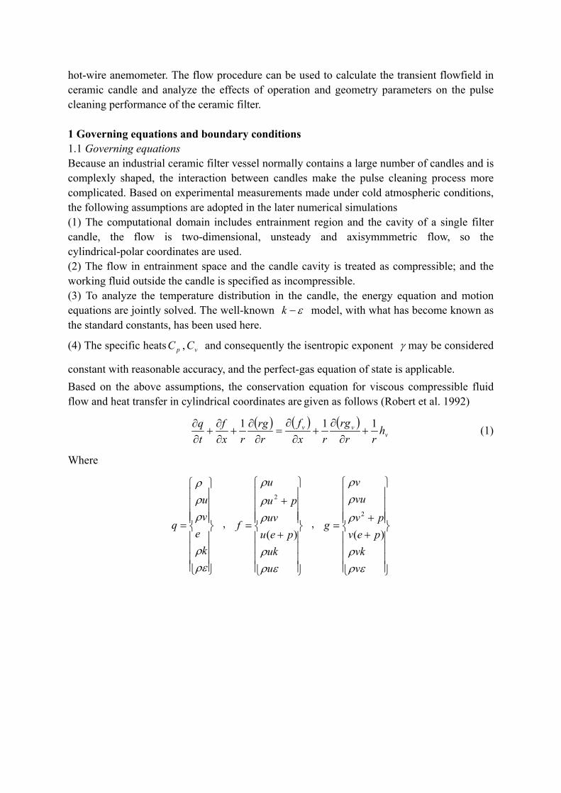
hot-wire anemometer. The flow procedure can be used to calculate the transient flowfield in ceramic candle and analyze the effects of operation and geometry parameters on the pulse cleaning performance of the ceramic filter. 1 Governing equations and boundary conditions 1.1 Governing equations Because an industrial ceramic filter vessel normally contains a large number of candles and is complexly shaped, the interaction between candles make the pulse cleaning process more complicated. Based on experimental measurements made under cold atmospheric conditions, the following assumptions are adopted in the later numerical simulations (1) The computational domain includes entrainment region and the cavity of a single filter candle, the flow is two-dimensional, unsteady and axisymmmetric flow, so the cylindrical-polar coordinates are used. (2) The flow in entrainment space and the candle cavity is treated as compressible; and the working fluid outside the candle is specified as incompressible. (3) To analyze the temperature distribution in the candle, the energy equation and motion equations are jointly solved. The well-known ε−k model, with what has become known as the standard constants, has been used here.

(4) The specific heatsC ,C and consequently the isentropic exponent p v γ may be considered

constant with reasonable accuracy, and the perfect-gas equation of state is applicable. Based on the above assumptions, the conservation equation for viscous compressible fluid flow and heat transfer in cylindrical coordinates are given as follows (Robert et al. 1992)

( ) ( ) ( )v

vv hrr

rgrx

frrg

rxf

tq 111

+∂

∂+

∂∂

=∂

∂+

∂∂

+∂∂ (1)

Where

=

ρερ

ρρρ

ke

vu

q ， ，

+

+

=

ερρ

ρρ

ρ

uuk

peuuv

puu

f)(

2

++

=

ερρ

ρ

ρρ

vvk

pevpv

vuv

g)(

2

∂∂∂∂

∂∂

++=

x

xk

xTvuf

k

xrxx

xr

xx

v

εµ

µ

λττ

ττ

ε

0

，

∂∂∂∂

∂∂

++=

r

rk

rTvug

k

rrxr

rr

xr

v

εµ

µ

λττ

ττ

ε

0

，h

−=

ε

τθθ

rSrS

p

k

v 0

00

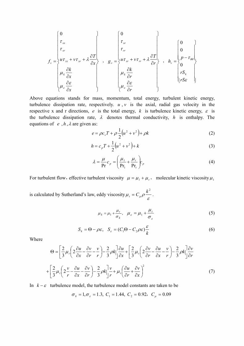
Above equations stands for mass, momentum, total energy, turbulent kinetic energy, turbulence dissipation rate, respectively. u , is the axial, radial gas velocity in the respective x and r directions, is the total energy, is turbulence kinetic energy,

ve k ε is

the turbulence dissipation rate, λ denotes thermal conductivity, is enthalpy. The equations of , ,

he h λ are given as：

( ) kvuTce v ρρρ +++= 22

21 (2)

( ) kvuTch p +++= 22

21 (3)

pt

tp cc

+==

PrPrPr 1

1 µµµλ (4)

For turbulent flow，effective turbulent viscosity tl µµµ += ， molecular kinetic viscosity 1µ

is calculated by Sutherland’s law, eddy viscosityε

ρµ µ

2kCt = .

,1k

tk σ

µµµ +=

εε σ

µµµ t+= 1 (5)

,ρε−Θ=kS k

CCS ερεε )( 21 −Θ= (6)

Where

rvk

rv

xu

rv

xuk

rv

rv

xu

tt ∂∂

−

−

∂∂

−∂∂

+∂∂

−

−

∂∂

−∂∂

=Θ ρµρµ322

32

322

32

2

322

32

∂∂

+∂∂

+

−

∂∂

−∂∂

−+xv

ru

rvk

rv

xu

rv

tt µρµ (7)

In ε−k turbulence model, the turbulence model constants are taken to be

09.092.0 ,44.1 ,3.1,1 21 ===== µεσσ CCCk ，

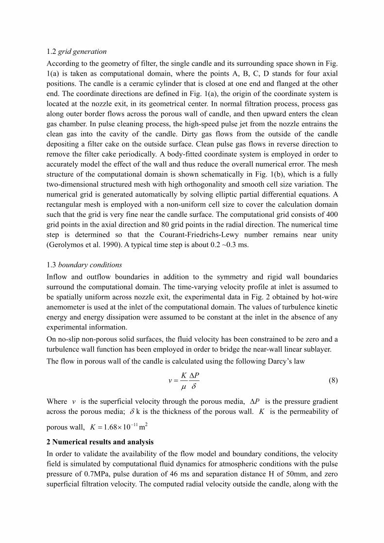
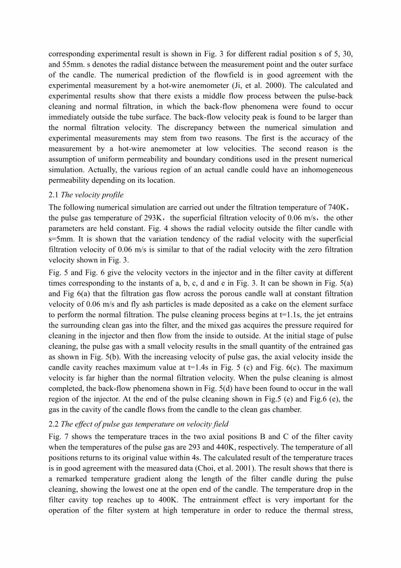
1.2 grid generation According to the geometry of filter, the single candle and its surrounding space shown in Fig. 1(a) is taken as computational domain, where the points A, B, C, D stands for four axial positions. The candle is a ceramic cylinder that is closed at one end and flanged at the other end. The coordinate directions are defined in Fig. 1(a), the origin of the coordinate system is located at the nozzle exit, in its geometrical center. In normal filtration process, process gas along outer border flows across the porous wall of candle, and then upward enters the clean gas chamber. In pulse cleaning process, the high-speed pulse jet from the nozzle entrains the clean gas into the cavity of the candle. Dirty gas flows from the outside of the candle depositing a filter cake on the outside surface. Clean pulse gas flows in reverse direction to remove the filter cake periodically. A body-fitted coordinate system is employed in order to accurately model the effect of the wall and thus reduce the overall numerical error. The mesh structure of the computational domain is shown schematically in Fig. 1(b), which is a fully two-dimensional structured mesh with high orthogonality and smooth cell size variation. The numerical grid is generated automatically by solving elliptic partial differential equations. A rectangular mesh is employed with a non-uniform cell size to cover the calculation domain such that the grid is very fine near the candle surface. The computational grid consists of 400 grid points in the axial direction and 80 grid points in the radial direction. The numerical time step is determined so that the Courant-Friedrichs-Lewy number remains near unity (Gerolymos et al. 1990). A typical time step is about 0.2 ~0.3 ms.

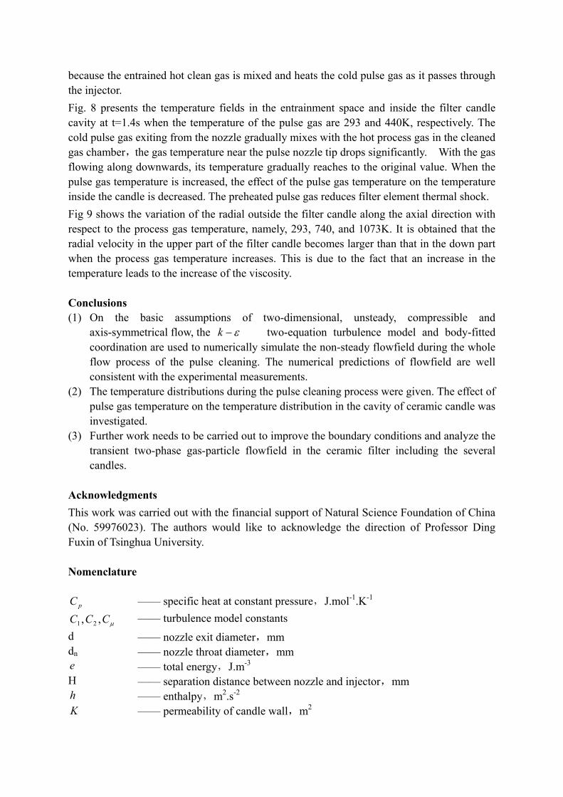
1.3 boundary conditions Inflow and outflow boundaries in addition to the symmetry and rigid wall boundaries surround the computational domain. The time-varying velocity profile at inlet is assumed to be spatially uniform across nozzle exit, the experimental data in Fig. 2 obtained by hot-wire anemometer is used at the inlet of the computational domain. The values of turbulence kinetic energy and energy dissipation were assumed to be constant at the inlet in the absence of any experimental information. On no-slip non-porous solid surfaces, the fluid velocity has been constrained to be zero and a turbulence wall function has been employed in order to bridge the near-wall linear sublayer. The flow in porous wall of the candle is calculated using the following Darcy’s law

δµPKv ∆

= (8)

Where is the superficial velocity through the porous media, v P∆ is the pressure gradient across the porous media; δ k is the thickness of the porous wall. K is the permeability of

porous wall, m11−1068.1 ×=K 2

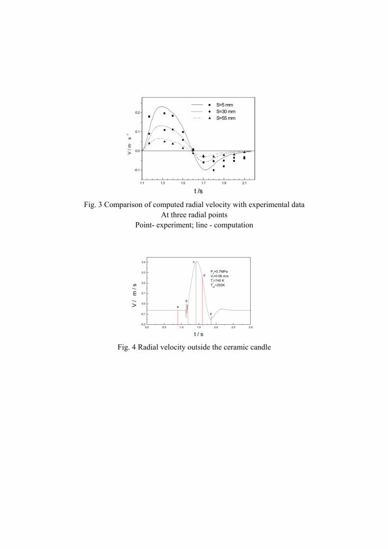
2 Numerical results and analysis In order to validate the availability of the flow model and boundary conditions, the velocity field is simulated by computational fluid dynamics for atmospheric conditions with the pulse pressure of 0.7MPa, pulse duration of 46 ms and separation distance H of 50mm, and zero superficial filtration velocity. The computed radial velocity outside the candle, along with the

corresponding experimental result is shown in Fig. 3 for different radial position s of 5, 30, and 55mm. s denotes the radial distance between the measurement point and the outer surface of the candle. The numerical prediction of the flowfield is in good agreement with the experimental measurement by a hot-wire anemometer (Ji, et al. 2000). The calculated and experimental results show that there exists a middle flow process between the pulse-back cleaning and normal filtration, in which the back-flow phenomena were found to occur immediately outside the tube surface. The back-flow velocity peak is found to be larger than the normal filtration velocity. The discrepancy between the numerical simulation and experimental measurements may stem from two reasons. The first is the accuracy of the measurement by a hot-wire anemometer at low velocities. The second reason is the assumption of uniform permeability and boundary conditions used in the present numerical simulation. Actually, the various region of an actual candle could have an inhomogeneous permeability depending on its location.

2.1 The velocity profile The following numerical simulation are carried out under the filtration temperature of 740K，

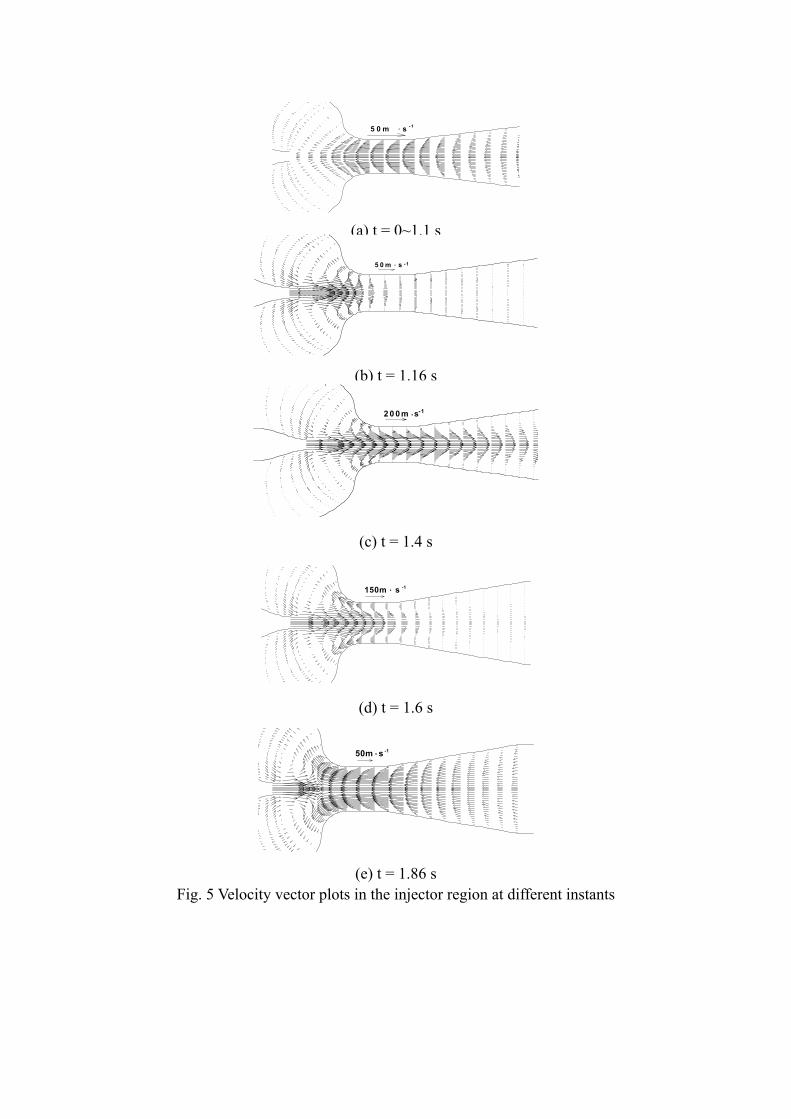
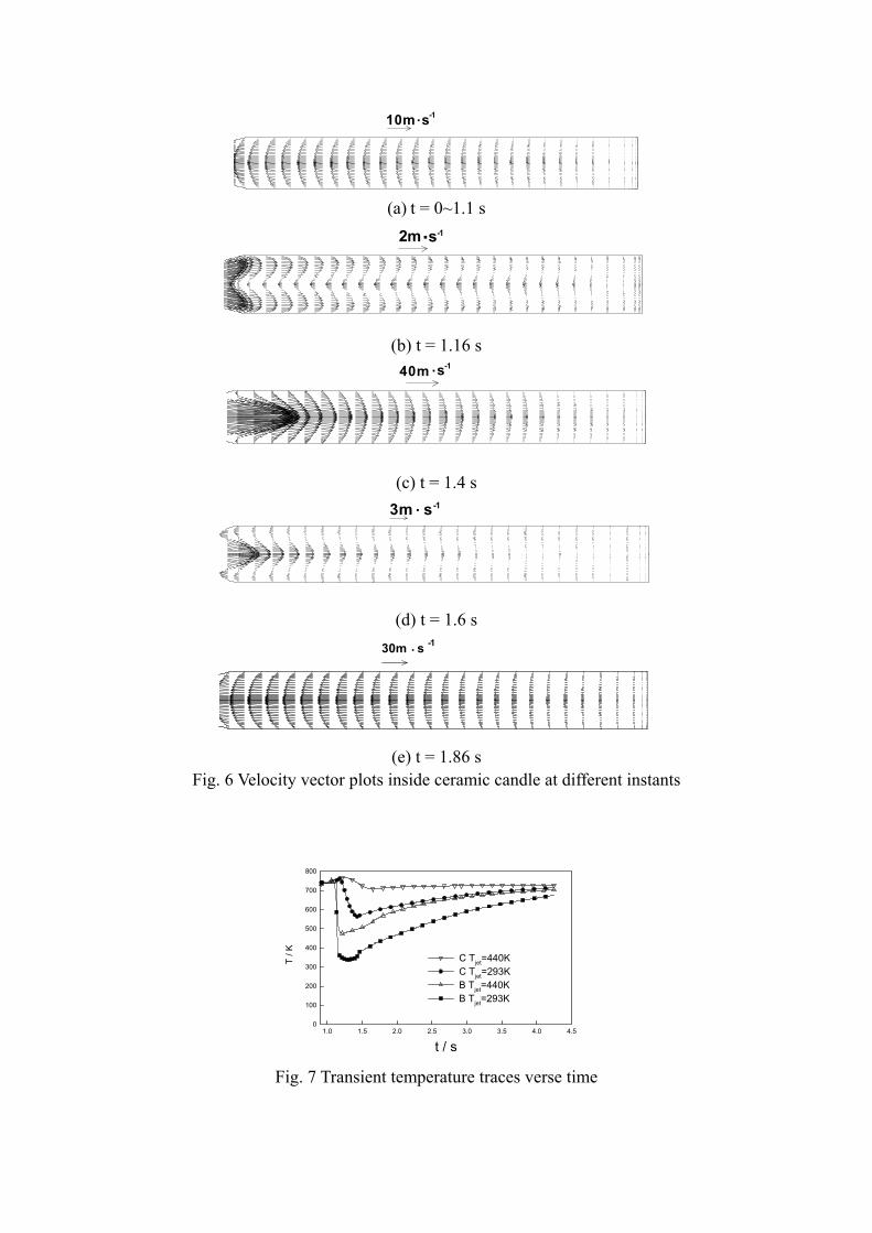
the pulse gas temperature of 293K，the superficial filtration velocity of 0.06 m/s，the other parameters are held constant. Fig. 4 shows the radial velocity outside the filter candle with s=5mm. It is shown that the variation tendency of the radial velocity with the superficial filtration velocity of 0.06 m/s is similar to that of the radial velocity with the zero filtration velocity shown in Fig. 3. Fig. 5 and Fig. 6 give the velocity vectors in the injector and in the filter cavity at different times corresponding to the instants of a, b, c, d and e in Fig. 3. It can be shown in Fig. 5(a) and Fig 6(a) that the filtration gas flow across the porous candle wall at constant filtration velocity of 0.06 m/s and fly ash particles is made deposited as a cake on the element surface to perform the normal filtration. The pulse cleaning process begins at t=1.1s, the jet entrains the surrounding clean gas into the filter, and the mixed gas acquires the pressure required for cleaning in the injector and then flow from the inside to outside. At the initial stage of pulse cleaning, the pulse gas with a small velocity results in the small quantity of the entrained gas as shown in Fig. 5(b). With the increasing velocity of pulse gas, the axial velocity inside the candle cavity reaches maximum value at t=1.4s in Fig. 5 (c) and Fig. 6(c). The maximum velocity is far higher than the normal filtration velocity. When the pulse cleaning is almost completed, the back-flow phenomena shown in Fig. 5(d) have been found to occur in the wall region of the injector. At the end of the pulse cleaning shown in Fig.5 (e) and Fig.6 (e), the gas in the cavity of the candle flows from the candle to the clean gas chamber.

2.2 The effect of pulse gas temperature on velocity field Fig. 7 shows the temperature traces in the two axial positions B and C of the filter cavity when the temperatures of the pulse gas are 293 and 440K, respectively. The temperature of all positions returns to its original value within 4s. The calculated result of the temperature traces is in good agreement with the measured data (Choi, et al. 2001). The result shows that there is a remarked temperature gradient along the length of the filter candle during the pulse cleaning, showing the lowest one at the open end of the candle. The temperature drop in the filter cavity top reaches up to 400K. The entrainment effect is very important for the operation of the filter system at high temperature in order to reduce the thermal stress,

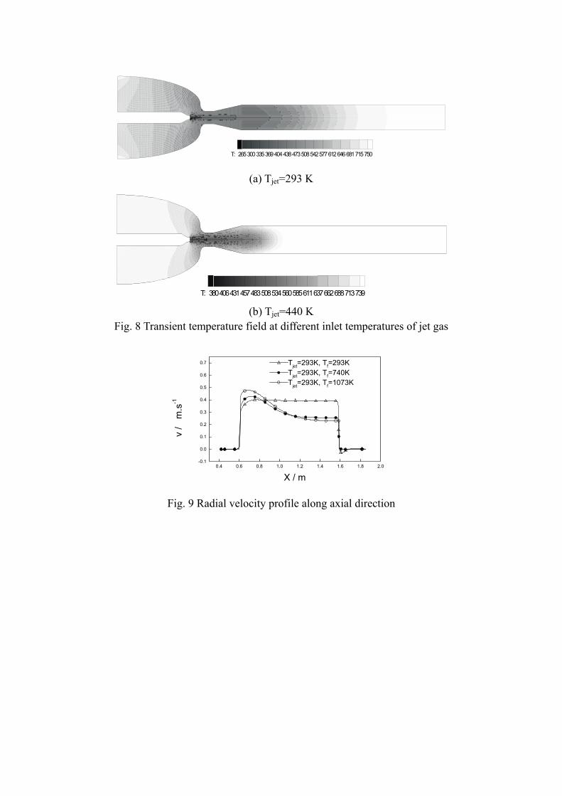
because the entrained hot clean gas is mixed and heats the cold pulse gas as it passes through the injector. Fig. 8 presents the temperature fields in the entrainment space and inside the filter candle cavity at t=1.4s when the temperature of the pulse gas are 293 and 440K, respectively. The cold pulse gas exiting from the nozzle gradually mixes with the hot process gas in the cleaned gas chamber，the gas temperature near the pulse nozzle tip drops significantly. With the gas flowing along downwards, its temperature gradually reaches to the original value. When the pulse gas temperature is increased, the effect of the pulse gas temperature on the temperature inside the candle is decreased. The preheated pulse gas reduces filter element thermal shock. Fig 9 shows the variation of the radial outside the filter candle along the axial direction with respect to the process gas temperature, namely, 293, 740, and 1073K. It is obtained that the radial velocity in the upper part of the filter candle becomes larger than that in the down part when the process gas temperature increases. This is due to the fact that an increase in the temperature leads to the increase of the viscosity. Conclusions (1) On the basic assumptions of two-dimensional, unsteady, compressible and

axis-symmetrical flow, the ε−k two-equation turbulence model and body-fitted coordination are used to numerically simulate the non-steady flowfield during the whole flow process of the pulse cleaning. The numerical predictions of flowfield are well consistent with the experimental measurements.

(2) The temperature distributions during the pulse cleaning process were given. The effect of pulse gas temperature on the temperature distribution in the cavity of ceramic candle was investigated.

(3) Further work needs to be carried out to improve the boundary conditions and analyze the transient two-phase gas-particle flowfield in the ceramic filter including the several candles.

Acknowledgments This work was carried out with the financial support of Natural Science Foundation of China (No. 59976023). The authors would like to acknowledge the direction of Professor Ding Fuxin of Tsinghua University.

Nomenclature

pC —— specific heat at constant pressure，J.mol-1.K-1

µCCC ,, 21 —— turbulence model constants d —— nozzle exit diameter，mm dn —— nozzle throat diameter，mm e —— total energy，J.m-3 H —— separation distance between nozzle and injector，mm h —— enthalpy，m2.s-2 K —— permeability of candle wall，m2

k —— turbulence kinetic energy，m2.s-2 P —— pressure of pulse gas，MPa p —— static pressure ，Pa r —— radial coordinate，m x —— axial coordinate，m s —— the distance between the measurement point and the outer surface of

candle wall，mm T —— temperature，K u

——axial velocity component，m.s-1

v —— radial velocity component，m.s-1 ε ——turbulence dissipation rate，m2.s-3 Θ —— production term in turbulent kinetic energy equation，kg.m-1.s-3

lt µµµ ,, —— effective viscosity, turbulent viscosity and molecular viscosity，kg.m-3

ρ —— gas density，kg.m-3

τ —— pulse duration，ms

Subscripts f ——filtration gas

jet ——pulse gas l —— laminar flow t —— turbulent flow

References Choi J-H, Seo Y-G, Chung J-W. 2001. Experimental Study on the Nozzle Effect of the Pulse Cleaning for the Ceramic Filter Candle. Powder Technology 114(1-3): 129-135 Christ A, Renz U, 1996. Numerical Simulation of Single Ceramic Filter Element Cleaning. In: Schmidt E, Gang T, Dittler A, eds. Proceedings of the 3rd High Temperature Gas Cleaning. Karlsruhe: Braun printconsult, 728-739 Gerolymos G.A., 1990. Implicit Multiple-Grid Solution of the Compressible Navier-Stokes Equations Using the ε−k Turbulence Closure. AIAA J., 28(10): 1707-1717 Gross R, Hecken M, Renz U, 1999. Hot Gas Filtration with Ceramic Filter Candles: Experimental and Numerical Investigations on Fluid Flow during Element Cleaning. In: Dittler A, Hemmer G, Kasper G, eds. Proceedings of the 4th High Temperature Gas Cleaning. Karlsruhe: Braun printconsult. 862-873 Ito S, Tanaka T, Kawamura S, 1998. Changes in Pressure Loss and Face Velocity of Ceramic Candle Filters Caused by Reverse Cleaning in Hot Coal Gas Filtration. Powder Technology, 100(2): 32-40 Ji Zhongli，Ding Fuxin，Meng Xiangbo，Shi Mingxian, 2000. Instantaneous Velocity outside Filtration Element in Ceramic Filter. Journal of Chemical Industry and Engineering (China). 51(2): 165-168 Pitt R U, Leith A J. Pitt R U, Leith A J, 1991. A Simple Method to Predict the Operation of Flue Gas Filter Pulse Cleaning Systems. Proceedings of the 11th International Conference

(ASME) on Fluidized Bed Combustion, Montreal, Canada, 1267-1281 Robert F. Kunz, Budugur Lakshminarayana, 1992. Explicit Navier-Stokes Computation of Cascade Flows Using the ε−k Turbulence Model. AIAA J. 30(1): 13-21

(a) (b) Fig. 1 Schematic diagram of ceramic candle and computational grid

0.00 0.50 1.00 1.50 2.00 2.50 3.000.0

50.0

100.0

150.0

200.0

250.0

300.0

P=0.7 MPa τ=46 msdn=6 mm d=17mm

v /

m.s

-1

t / s

Fig. 2 Jet velocity traces verse time

1.1 1.3 1.5 1.7 1.9 2.1

-0.1

0.0

0.1

0.2

S=5 mm S=30 mm S=55 mm

V / m

·s

-1

t /s Fig. 3 Comparison of computed radial velocity with experimental data

At three radial points Point- experiment; line - computation

0.0 0.5 1.0 1.5 2.0 2.5 3.0-0.2

-0.1

0.0

0.1

0.2

0.3

0.4

e

d

c

ba

P0=0.7MPaVf=0.06 m/sTf=740 KTjet=293K

V /

m /

s

t / s

Fig. 4 Radial velocity outside the ceramic candle

5 0 m . s -1

(a) t = 0~1.1 s

5 0 m . s -1

(b) t = 1.16 s

200m .s-1

(c) t = 1.4 s

150m . s -1

(d) t = 1.6 s

50m . s -1

(e) t = 1.86 s

Fig. 5 Velocity vector plots in the injector region at different instants

10m.s-1

(a) t = 0~1.1 s 2m.s-1

(b) t = 1.16 s 40m .s-1

(c) t = 1.4 s

3m . s-1

(d) t = 1.6 s

30m . s -1

(e) t = 1.86 s

Fig. 6 Velocity vector plots inside ceramic candle at different instants

1.0 1.5 2.0 2.5 3.0 3.5 4.0 4.50

100

200

300

400

500

600

700

800

C Tjet=440K C Tjet=293K B Tjet=440K B Tjet=293K

T / K

t / s

Fig. 7 Transient temperature traces verse time

T: 265300335369404438473508542577612646681715750

(a) Tjet=293 K

T: 380406431457483508534560585611637662688713739

(b) Tjet=440 K Fig. 8 Transient temperature field at different inlet temperatures of jet gas

0.4 0.6 0.8 1.0 1.2 1.4 1.6 1.8 2.0-0.1

0.0

0.1

0.2

0.3

0.4

0.5

0.6

0.7 Tjet=293K, Tf=293K Tjet=293K, Tf=740KTjet=293K, Tf=1073K

v /

m.s

-1

X / m

Fig. 9 Radial velocity profile along axial direction