Zhen Gao, Linglong Dai, Wei Dai, Byonghyo Shim, and ... massive MIMO systems, an accurate acquisition of the channel state information (CSI) is essential for signal detection, beamforming,

0090-6778 (c) 2015 IEEE. Personal use is permitted, but republication/redistribution requires IEEE permission. See http://www.ieee.org/publications_standards/publications/rights/index.html for more information.

This article has been accepted for publication in a future issue of this journal, but has not been fully edited. Content may change prior to final publication. Citation information: DOI 10.1109/TCOMM.2015.2508809, IEEETransactions on Communications

1

Structured Compressive Sensing Based Spatio-TemporalJoint Channel Estimation for FDD Massive MIMO

Zhen Gao, Linglong Dai, Wei Dai, Byonghyo Shim, and Zhaocheng Wang

Abstract—Massive MIMO is a promising technique for fu-ture 5G communications due to its high spectrum and energyefficiency. To realize its potential performance gain, accuratechannel estimation is essential. However, due to massive numberof antennas at the base station (BS), the pilot overhead requiredby conventional channel estimation schemes will be unafford-able, especially for frequency division duplex (FDD) massiveMIMO. To overcome this problem, we propose a structuredcompressive sensing (SCS)-based spatio-temporal joint channelestimation scheme to reduce the required pilot overhead, wherebythe spatio-temporal common sparsity of delay-domain MIMOchannels is leveraged. Particularly, we first propose the non-orthogonal pilots at the BS under the framework of CS theory toreduce the required pilot overhead. Then, an adaptive structuredsubspace pursuit (ASSP) algorithm at the user is proposed tojointly estimate channels associated with multiple OFDM symbolsfrom the limited number of pilots, whereby the spatio-temporalcommon sparsity of MIMO channels is exploited to improvethe channel estimation accuracy. Moreover, by exploiting thetemporal channel correlation, we propose a space-time adaptivepilot scheme to further reduce the pilot overhead. Additionally,we discuss the proposed channel estimation scheme in multi-cell scenario. Simulation results demonstrate that the proposedscheme can accurately estimate channels with the reduced pilotoverhead, and it is capable of approaching the optimal oracleleast squares estimator.

Index Terms—Massive MIMO, structured compressive sensing(SCS), frequency division duplex (FDD), channel estimation.

I. INTRODUCTION

MASSIVE MIMO employing a large number of anten-nas at the base station (BS) to simultaneously serve

multiple users, has recently emerged as a promising approachto realize high-throughput green wireless communications [1].By exploiting the large number of degrees of spatial freedom,massive MIMO can boost the system capacity and energyefficiency by orders of magnitude. Therefore, massive MIMOhas been widely recognized as a key enabling technique forfuture spectrum and energy efficient 5G communications [2].

In massive MIMO systems, an accurate acquisition ofthe channel state information (CSI) is essential for signaldetection, beamforming, resource allocation, etc. However, dueto massive antennas at the BS, each user has to estimate

Z. Gao, L. Dai, and Z. Wang are with Department of ElectronicEngineering, Tsinghua University, Beijing 100084, China (E-mails: [email protected]; daill, [email protected]).

W. Dai is with Department of Electrical and Electronic Engi-neering, Imperial College London, London SW7 2AZ, UK (E-mail:[email protected]).

B. Shim is with the Department of Electrical and Computer Engineering,Seoul National University, Seoul 151-742, Korea (E-mail:[email protected]).

This work was supported by the National Key Basic Research Programof China (Grant No. 2013CB329203), the National Natural Science Foun-dation of China (Grant Nos. 61571270 and 61201185), the Beijing NaturalScience Foundation (Grant No. 4142027), and the Foundation of Shenzhengovernment.

channels associated with hundreds of transmit antennas, whichresults in the prohibitively high pilot overhead. Hence, howto realize the accurate channel estimation with the affordablepilot overhead becomes a challenging problem, especially forfrequency division duplex (FDD) massive MIMO systems [3].To date, most of researches on massive MIMO sidestep thischallenge by assuming the time division duplex (TDD) proto-col, where the CSI in the uplink can be more easily acquiredat the BS due to the small number of single-antenna usersand the powerful processing capability of the BS, and then thechannel reciprocity property can be leveraged to directly obtainthe CSI in the downlink [4]. However, due to the calibrationerror of radio frequency chains and limited coherence time,the CSI acquired in the uplink may not be accurate for thedownlink [5], [6]. More importantly, compared with TDDsystems, FDD systems can provide more efficient communi-cations with low latency [7], and it has dominated currentcellular systems. Therefore, it is of importance to explore thechallenging problem of channel estimation for FDD massiveMIMO systems, which can facilitate massive MIMO to bebackward compatible with current FDD dominated cellularnetworks.

Recently, there have been extensive studies on channelestimation for conventional small-scale FDD MIMO systems[8]–[14]. It has been proven that the equi-spaced and equi-power orthogonal pilots can be optimal to estimate the non-correlated Rayleigh MIMO channels for one OFDM symbol,where the required pilot overhead increases with the number oftransmit antennas [8]. By exploiting the spatial correlation ofMIMO channels, the pilot overhead to estimate Rician MIMOchannels can be reduced [9]. Furthermore, by exploiting thetemporal channel correlation, further reduced pilot overheadcan be achieved to estimate MIMO channels associated withmultiple OFDM symbols [10], [11]. Currently, orthogonalpilots have been widely used in the existing MIMO systems,where the pilot overhead is not a big issue due to the smallnumber of transmit antennas (e.g., up to eight antennas inLTE-Advanced system) [12]–[14]. However, this issue can becritical in massive MIMO systems due to massive number ofantennas at the BS (e.g., 128 antennas or even more at theBS [2]).

In [15], an approach to exploit the temporal correlationand sparsity of delay-domain channels for the reduced pilotoverhead has been proposed for FDD massive MIMO systems,but the interference cancellation of training sequences ofdifferent transmit antennas will be difficult when the numberof transmit antennas is large. [16]–[18] leveraged the spatialcorrelation and sparsity of delay-domain MIMO channels toestimate channels with the reduced pilot overhead, but theassumption of the known channel sparsity level at the user is



2

unrealistic. By exploiting the spatial channel correlation, thecompressive sensing (CS)-based channel estimation schemeswere proposed in [19]–[21], but the leveraged spatial corre-lation can be impaired due to the non-ideal antenna array[3], [5]. [22] proposed an open-loop and closed-loop channelestimation scheme for massive MIMO, but the long-termchannel statistics perfectly known at the user can be difficult.

On the other hand, for typical broadband wireless commu-nication systems, delay-domain channels intrinsically exhibitthe sparse nature due to the limited number of significantscatterers in the propagation environments and large channeldelay spread [15], [23]–[29]. Meanwhile, for MIMO systemswith co-located antenna array at the BS, channels betweenone user and different transmit antennas at the BS exhibitvery similar path delays due to very similar scatterers in thepropagation environments, which indicates that delay-domainchannels between the user and different transmit antennas atthe BS share the common sparsity when the aperture of theantenna array is not very large [3], [30]. Moreover, sincethe path delays vary much slower than the path gains dueto the temporal channel correlation, such sparsity is almostunchanged during the coherence time [31]. In this paper,such channel properties of MIMO channels are referred toas the spatio-temporal common sparsity, which is usually notconsidered in most of current work.

In this paper, by exploiting the spatio-temporal commonsparsity of delay-domain MIMO channels, we propose astructured compressive sensing (SCS)-based spatio-temporaljoint channel estimation scheme with significantly reducedpilot overhead for FDD massive MIMO systems. Specifically,at the BS, we propose a non-orthogonal pilot scheme underthe framework of CS theory, which is essentially differentfrom the widely used orthogonal pilots under the frameworkof classical Nyquist sampling theorem. Compared with con-ventional orthogonal pilots, the proposed non-orthogonal pilotscheme can substantially reduce the required pilot overhead forchannel estimation. At the user side, we propose an adaptivestructured subspace pursuit (ASSP) algorithm for channelestimation, whereby the spatio-temporal common sparsity ofdelay-domain MIMO channels is leveraged to improve thechannel estimation performance from the limited numberof pilots. Furthermore, by leveraging the temporal channelcorrelation, we propose a space-time adaptive pilot schemeto realize the accurate channel estimation with further reducedpilot overhead, where the specific pilot signals should considerthe geometry of antenna array at the BS and the mobilityof served users. Additionally, we further extend the proposedchannel estimation scheme from the single-cell scenario tothe multi-cell scenario. Finally, simulation results verify thatthe proposed scheme outperforms its conventional counterpartswith reduced pilot overhead, where the performance of theSCS-based channel estimation scheme approaches that of theoracle least squares (LS) estimator.

The rest of the paper is organized as follows. Section II il-lustrates the spatio-temporal common sparsity of delay-domainMIMO channels. In Section III, the proposed SCS-basedspatio-temporal joint channel estimation scheme is discussedin detail. In Section IV, we provide the performance analysis.

Section V shows the simulation results. Finally, Section VIconcludes this paper.

Notation: Boldface lower and upper-case symbols representcolumn vectors and matrices, respectively. The operator represents the Hadamard product, ⌊·⌋ denotes the integer flooroperator, and diagx is a diagonal matrix with elements of xon its diagonal. The matrix inversion, transpose, and Hermitiantranspose operations are denoted by (·)−1, (·)T, and (·)H,respectively, while (·)† denotes the Moore-Penrose matrixinversion. | · |c denotes the cardinality of a set, the l2-normoperation and Frobenius-norm operation are given by ∥ · ∥2and ∥ · ∥F , respectively. Ωc denotes the complementary set ofthe set Ω. Tr· is the trace of a matrix. ⟨·, ·⟩ is the Frobeniusinner product, and ⟨A,B⟩= TrAHB. Finally, Φ(l) denotesthe lth column vector of the matrix Φ.

II. SPATIO-TEMPORAL COMMON SPARSITY OFDELAY-DOMAIN

Extensive experimental studies have shown that wirelessbroadband channels exhibit the sparsity in the delay domain.This is caused by the fact that the number of multipathdominating the majority of channel energy is small due to thelimited number of significant scatterers in the wireless signalpropagation environments, while the channel delay spread canbe large due to the large difference between the time ofarrival (ToA) of the earliest multipath and the ToA of thelatest multipath [15], [23]–[29]. Specifically, in the downlink,the delay-domain channel impulse response (CIR) betweenthe mth transmit antenna at the BS and one user can beexpressed as

hm,r = [hm,r[1], hm,r[2], · · · , hm,r[L]]T, 1 ≤ m ≤ M, (1)

where r is the index of the OFDM symbol in the time domain,L is the equivalent channel length, Dm,r = supphm,r =l : |hm,r[l]| > pth, 1 ≤ l ≤ L is the support set of hm,r, andpth is the noise floor according to [32]. The sparsity levelof wireless channels is denoted as Pm,r = |Dm,r|c, and wehave Pm,r ≪ L due to the sparse nature of delay-domainchannels [15], [23], [24], [26]1.

Moreover, there are measurements showing that CIRs be-tween different transmit antennas and one user exhibit verysimilar path delays [3], [30]. The reason is that, in typicalmassive MIMO geometry, the scale of the compact antennaarray at the BS is relatively small compared with the largesignal transmission distance, and channels associated withdifferent transmit-receive antenna pairs share the commonscatterers. Therefore, the sparsity patterns of CIRs of differenttransmit-receive antenna pairs have a large overlap. Moreover,for MIMO systems with not very large M , these CIRs canshare the common sparse pattern [3], [17], [30], i.e.,

D1,r = D2,r = · · · = DM,r, (2)

1The sparse delay-domain channels may exhibit the power leakage dueto the non-integer normalized path delays. To solve this issue, there havebeen off-the-shelf techniques to mitigate the power leakage [28], [29]. Forconvenience, we consider the sparse channel model in the equivalent discrete-time baseband widely used in CS-based channel estimation [15], [23], [24],[26].



3

Dif

fere

nt

Use

rs

Time (different OFDM symbols within coherence time)

Space

(diff

erent tra

nsmit

anten

nas)

CIRs

BS

User 1

User 2

User 2

User 1

(a)

(b)

Fig. 1. Spatio-temporal common sparsity of delay-domain MIMO channels:(a) Wireless channels exhibit the sparse nature due to the limited number ofscatterers; (b) Delay-domain MIMO channels between the co-located antennaarray and one user exhibit the spatio-temporal common sparsity.

which is referred to as the spatial common sparsity of wirelessMIMO channels. For example, we consider the LTE-Advancedsystem working at a carrier frequency of fc = 2 GHz witha signal bandwidth of fs = 10 MHz, and the uniform lineararray (ULA) with the antenna spacing of half-wavelength. Fortwo transmit antennas with the distance of 8 half-wavelengths,their maximum difference of path delays from the commonscatterer is 8λ/2

c = 4/fc = 0.002 µs, which is negligiblecompared with the system sample period Ts = 1/fs = 0.1 µs,where λ and c are the wavelength and the velocity of light,respectively. It should be pointed out that the path gains ofdifferent transmit-receive antenna pairs from the same scatterercan be different or even uncorrelated due to the non-isotropicantennas2 [5].

Finally, practical wireless channels also exhibit the temporalcorrelation even in fast time-varying scenarios [31]. It hasbeen demonstrated that the path delays usually vary muchslower than the path gains [31]. In other words, although thepath gains can vary significantly from one OFDM symbolto another, the path delays remain almost unchanged duringseveral successive OFDM symbols. This is due to the fact thatthe coherence time of path gains over time-varying channelsis inversely proportional to the system carrier frequency, whilethe duration for path delay variation is inversely proportionalto the system bandwidth [31]. For example, in the LTE-

2For practical massive MIMO systems, different antennas at the BS withdifferent directivities can destroy the spatial correlation of path gains overdifferent transmit-receive pairs from the same scatterer and improve the systemcapacity [3]. However, this spatial channel correlation is usually exploited inconventional channel estimation schemes for reduced pilot overhead, whichcan be unrealistic.

…

!"

Fig. 2. Pilot designs for massive MIMO with M = 64 in one time-frequencyresource block. (a) Conventional orthogonal pilot design; (b) Proposed non-orthogonal pilot design.

Advanced system with fc = 2 GHz and fs = 10 MHz, thepath delays vary at a rate that is about several hundred timesslower than that of the path gains [15]. That is to say, duringthe coherence time of path delays, CIRs associated with Rsuccessive OFDM symbols have the common sparsity due tothe almost unchanged path delays, i.e.,

Dm,r = Dm,r+1 = · · · = Dm,r+R−1, 1 ≤ m ≤ M. (3)

This temporal correlation of wireless channels is also referredto as the temporal common sparsity of wireless channels inthis paper.

The spatial and temporal channel correlations discussedabove are jointly referred to as the spatio-temporal commonsparsity of delay-domain MIMO channels, which can beillustrated in Fig. 1. This channel property is usually notconsidered in existing channel estimation schemes. In thispaper, we will exploit this channel property to overcome thechallenging problem of channel estimation for FDD massiveMIMO.

III. PROPOSED SCS-BASED SPATIO-TEMPORAL JOINTCHANNEL ESTIMATION SCHEME

In this section, the SCS-based spatio-temporal joint channelestimation scheme is proposed for FDD massive MIMO.First, we propose the non-orthogonal pilot scheme at the BSto reduce the pilot overhead. Then, we propose the ASSPalgorithm at the user for reliable channel estimation. Moreover,we propose the space-time adaptive pilot scheme for furtherreduction of the pilot overhead. Finally, we briefly discuss theproposed channel estimation scheme extended to multi-cellscenario.

A. Non-Orthogonal Pilot Scheme at the BS

The design of conventional orthogonal pilots is based onthe framework of classical Nyquist sampling theorem, andthis design has been widely used in the existing MIMOsystems. The orthogonal pilots can be illustrated in Fig. 2(a), where pilots associated with different transmit antennasoccupy the different subcarriers. For massive MIMO systemswith hundreds of transmit antennas, such orthogonal pilots willsuffer from the prohibitively high pilot overhead.

In contrast, the design of the proposed non-orthogonal pilotscheme, as shown in Fig. 2 (b), is based on CS theory, andit allows pilots of different transmit antennas to occupy thecompletely same subcarriers. By leveraging the sparse nature



4

of channels, the pilots used for channel estimation can bereduced substantially.

For the proposed non-orthogonal pilot scheme, we first con-sider the MIMO channel estimation for one OFDM symbol asan example. Particularly, we denote the index set of subcarriersallocated to pilots as ξ, which is uniquely selected from the setof 1, 2, · · · , N and identical for all transmit antennas. HereNp = |ξ|c is the number of pilot subcarriers in one OFDMsymbol, and N is the number of subcarriers in one OFDMsymbol. Moreover, we denote the pilot sequence of the mthtransmit antenna as pm ∈ CNp×1. The specific pilot design ξand pmMm=1 will be detailed in Section IV-A .

B. SCS-Based Channel Estimation at the User

At the user, after the removal of the guard interval anddiscrete Fourier transformation (DFT), the received pilot se-quence yr ∈ CNp×1 of the rth OFDM symbol can beexpressed as

yr =M∑

m=1diagpmF|ξ

[hm,r

0(N−L)×1

]+wr

=M∑

m=1PmFL|ξhm,r +wr =

M∑m=1

Φmhm,r +wr,

(4)where Pm= diagpm, F ∈ CN×N is a DFT matrix, FL ∈CN×L is a partial DFT matrix consisted of the first L columnsof F, F|ξ ∈ CNp×N and FL|ξ ∈ CNp×L are the sub-matricesby selecting the rows of F and FL according to ξ, respectively,wr ∈ CNp×1 is the additive white Gaussian noise (AWGN)vector in the rth OFDM symbol, and Φm = PmFL|ξ.Moreover, (4) can be rewritten in a more compact form as

yr = Φhr +wr, (5)

where Φ = [Φ1,Φ2, · · · ,ΦM ] ∈ CNp×ML, and hr =[hT

1,r,hT2,r, · · · ,hT

M,r]T ∈ CML×1 is an aggregate CIR vector.

For massive MIMO systems, we usually have Np ≪ MLdue to the large number of transmit antennas M and the limitednumber of pilots Np. This indicates that we cannot reliablyestimate hr from yr using conventional channel estimationschemes, since (5) is an under-determined system. However,the observation that hr is a sparse signal due to the sparsityof hm,rMm=1 inspires us to estimate the sparse signal hr ofhigh dimension from the received pilot sequence yr of lowdimension under the framework of CS theory [33]. Moreover,the inherently spatial common sparsity of wireless MIMOchannels can be also exploited for performance enhancement.Specifically, we rearrange the aggregate CIR vector hr toobtain the equivalent CIR vector dr as

dr = [dT1,r,d

T2,r, · · · ,dT

L,r]T ∈ CML×1, (6)

where dl,r = [h1,r[l], h2,r[l], · · · , hM,r[l]]T for 1 ≤ l ≤ L.

Similarly, Φ can be rearranged as Ψ, i.e.,

Ψ = [Ψ1,Ψ2, · · · ,ΨL] ∈ CNp×ML, (7)

where Ψl =[Φ

(l)1 ,Φ

(l)2 , · · · ,Φ(l)

M

]=

[ψ1,l,ψ2,l, · · · ,ψM,l] ∈ CNp×M . In this way, (5) canbe reformulated as

yr = Ψdr +wr. (8)

From (8), it can be observed that due to the spatial commonsparsity of wireless MIMO channels, the equivalent CIR vectordr exhibits the structured sparsity [33].

Furthermore, the temporal correlation of wireless channelsindicates that such spatial common sparsity in MIMO systemsremains virtually unchanged over R successive OFDM sym-bols, where R is determined by the coherence time of thepath delays [15]. Hence, wireless MIMO channels exhibit thespatio-temporal common sparsity during R successive OFDMsymbols. Considering (8) during R adjacent OFDM symbolswith the same pilot pattern, we have

Y = ΨD+W, (9)where Y = [yr,yr+1,· · ·,yr+R−1] ∈ CNp×R is the measure-ment matrix, D =

[dr,dr+1,· · ·,dr+R−1

]∈ CML×R is the

equivalent CIR matrix, and W = [wr,wr+1, · · · ,wr+R−1] ∈CNp×R is the AWGN matrix. It should be pointed out that Dcan be expressed as

D = [DT1 ,D

T2 , · · · ,DT

L]T, (10)

where Dl for 1 ≤ l ≤ L has the size of M ×R, and the mthrow and rth column element of Dl is the channel gain of thelth path delay associated with the mth transmit antenna in therth OFDM symbol.

It is clear that the equivalent CIR matrix D in (10) exhibitsthe structured sparsity due to the spatio-temporal commonsparsity of wireless MIMO channels, and this intrinsic sparsityin D can be exploited for better channel estimation perfor-mance. In this way, we can jointly estimate channels associatedwith M transmit antennas in R OFDM symbols by jointlyprocessing the received pilots of R OFDM symbols.

By exploiting the structured sparsity of D in (9), we proposethe ASSP algorithm as described in Algorithm 1 to estimatechannels for massive MIMO systems. Developed from theclassical subspace pursuit (SP) algorithm [34], the proposedASSP algorithm exploits the structured sparsity of D forfurther improved sparse signal recovery performance.

For Algorithm 1, some notations should be further detailed.First, both Z ∈ CML×R and

D ∈ CML×R are consist-ed of L sub-matrices with the equal size of M ×R, i.e.,Z = [ZT

1 ,ZT2 , · · · ,ZT

L]T and

D = [

DT1 ,

DT2 , · · · ,

DTL]

T.

Second, we have

DΩ =

[

DT

Ω(1),

DT

Ω(2), · · · ,

DT

Ω(|Ω|c)

]Tand

ΨΩ =[Ψ

Ω(1),Ψ

Ω(2), · · · ,Ψ

Ω(|Ω|c)

], where Ω(1) < Ω(2) <

· · · < Ω(|Ω|c) are elements in the set Ω. Third, Πs (·) is aset, whose elements are the indices of the largest s elementsof its argument. Finally, to reliably acquire the channel spar-sity level, we stop the iteration if

∥∥Rk∥∥F

> ∥Rs−1∥F or∥∥∥

Dl

∥∥∥F

≤√MRpth, where

∥∥∥

Dl

∥∥∥F

is the smallest∥∥∥

Dl

∥∥∥F

for l ∈ Ωk, and pth is the noise floor according to [32]. Theproposed stopping criteria will be further discussed in SectionIV-B.

Here we further explain the main steps in Algorithm 1 asfollows. First, for step 2.1∼2.7, the ASSP algorithm aims toacquire the solution D to (9) with the fixed sparsity level s ina greedy way, which is similar to the classical SP algorithm.Second,

∥∥Rk−1∥∥F

≤∥∥Rk

∥∥F

indicates that the s-sparse



5

Algorithm 1 Proposed ASSP Algorithm.Input: Noisy measurement matrix Y and sensing matrix Ψ.Output: The estimation of channels hm,tm=M,t=r+R−1

m=1,t=r .• Step 1 (Initialization) The initial channel sparsity level s = 1,

the iterative index k = 1, the support set Ωk−1 = ∅, and theresidual matrices Rk−1 = Y and ∥Rs−1∥F = + inf .

• Step 2 (Solve the Structured Sparse Matrix D to (9))repreat1. (Correlation) Z = ΨHRk−1;2. (Support Estimate) Ω

′k = Ωk−1 ∪Πs(

∥Zl∥FL

l=1

);

3. (Support Pruning)

DΩ′k = Ψ†

Ω′kY;

D(Ω′k)c = 0;

Ωk = Πs

(∥∥∥

Dl

∥∥∥F

L

l=1

);

4. (Matrix Estimate)

DΩk = Ψ†ΩkY;

D(Ωk)c = 0;

5. (Residue Update) Rk = Y −Ψ

D;

6. (Matrix Update)

Dk

=

D;if∥∥Rk−1

∥∥F>

∥∥Rk∥∥F

7. (Iteration with Fixed Sparsity Level) Ωk = Ωk; k = k + 1;else

8. (Update Sparsity Level)

Ds =

Dk−1

; Rs = Rk−1;Ωs = Ωk−1; s = s+ 1;

end ifuntil stopping criteria are met

• Step 3 (Obtain Channels) D =

Ds−1 and obtain the estimationof channels hm,tm=M,t=r+R−1

m=1,t=r according to (4)-(9).

solution D to (9) has been obtained, and then the sparsitylevel is updated to find the (s+1)-sparse solution D. Finally,if the stopping criteria are met, the iteration quits, and weconsider the estimated solution to (9) with the last sparsitylevel as the estimated channels, i.e., D =

Ds−1.Compared to the SP algorithm and the model-based SP al-

gorithm [35], the proposed ASSP algorithm has the followingdistinctive features:

• The classical SP algorithm reconstructs one high-dimensional sparse vector from one low-dimensionalmeasurement vector without exploiting the structured s-parsity of the sparse vector. The model-based SP algorith-m reconstructs one high-dimensional sparse vector fromone low-dimensional measurement vector by exploitingthe structured sparsity of the sparse vector for improvedperformance. In contrast, the proposed ASSP algorithmrecovers the high-dimensional sparse matrix with theinherently structured sparsity from the low-dimensionalmeasurement matrix, whereby the inherently structuredsparsity of the sparse matrix is exploited for the improvedmatrix reconstruction performance.

• Both the classical SP algorithm and model-based SP al-gorithm require the sparsity level as the priori informationfor reliable sparse signal reconstruction. In contrast, theproposed ASSP algorithm does not need this priori infor-mation, since it can adaptively acquire the sparsity levelof the structured sparse matrix. By exploiting the practicalphysical property of wireless channels, the proposed stop-ping criteria enable ASSP algorithm to estimate channelswith good mean square error (MSE) performance, whichwill be detailed in Section IV-B. Moreover, simulation

R2

R1

R64

+

+

+

Time

Fre

quen

cy

Pilot of 1st

TA

Pilot of 2nd

TA

Pilot of 64th TA

Data block

R128

+

+

+

Pilot of 65th

TA

Pilot of 66th TA

Pilot of 128th

TA

R65

R66

(a)

(b)

2-D Antenna Array at the BS

1st ~64th TA 65th ~128th TA

fd

The 1st antenna group The 2nd antenna group

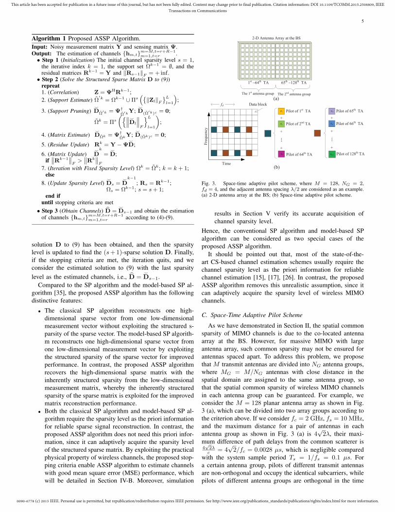
Fig. 3. Space-time adaptive pilot scheme, where M = 128, NG = 2,fd = 4, and the adjacent antenna spacing λ/2 are considered as an example.(a) 2-D antenna array at the BS; (b) Space-time adaptive pilot scheme.

results in Section V verify its accurate acquisition ofchannel sparsity level.

Hence, the conventional SP algorithm and model-based SPalgorithm can be considered as two special cases of theproposed ASSP algorithm.

It should be pointed out that, most of the state-of-the-art CS-based channel estimation schemes usually require thechannel sparsity level as the priori information for reliablechannel estimation [15], [17], [26]. In contrast, the proposedASSP algorithm removes this unrealistic assumption, since itcan adaptively acquire the sparsity level of wireless MIMOchannels.

C. Space-Time Adaptive Pilot Scheme

As we have demonstrated in Section II, the spatial commonsparsity of MIMO channels is due to the co-located antennaarray at the BS. However, for massive MIMO with largeantenna array, such common sparsity may not be ensured forantennas spaced apart. To address this problem, we proposethat M transmit antennas are divided into NG antenna groups,where MG = M/NG antennas with close distance in thespatial domain are assigned to the same antenna group, sothat the spatial common sparsity of wireless MIMO channelsin each antenna group can be guaranteed. For example, weconsider the M = 128 planar antenna array as shown in Fig.3 (a), which can be divided into two array groups according tothe criterion above. If we consider fc = 2 GHz, fs = 10 MHz,and the maximum distance for a pair of antennas in eachantenna group as shown in Fig. 3 (a) is 4

√2λ, their maxi-

mum difference of path delays from the common scatterer is4√2λc = 4

√2/fc = 0.0028 µs, which is negligible compared

with the system sample period Ts = 1/fs = 0.1 µs. Fora certain antenna group, pilots of different transmit antennasare non-orthogonal and occupy the identical subcarriers, whilepilots of different antenna groups are orthogonal in the time



6

domain or frequency domain, which can be illustrated in Fig.3 (b). For the specific parameter NG, we should consider thegeometry and scale of the antenna array at the BS, fc, and fs.

On the other hand, wireless MIMO channels exhibit thetemporal correlation. Such temporal channel correlation indi-cates that during the coherence time of path gains, channelsin several successive OFDM symbols can be considered to bequasi-static, and the channel estimation in one OFDM symbolcan be used to estimate channels of several adjacent OFDMsymbols. This motivates us to further reduce the pilot overheadand increase the available spectrum and energy resources foreffective data transmission. To be specific, as illustrated in Fig.3, every fd adjacent OFDM symbols share the common pilots,where fd is determined by the coherence time of path gainsor the mobility of served users.

By exploiting such temporal channel correlation, we can uselarge fd to reduce the pilot overhead. To estimate channelsof OFDM symbols without pilots, we can use interpolationalgorithms according to the estimated channels of adjacentOFDM symbols with pilots, e.g., we can adopt the linearinterpolation algorithm as follows

hm,r = [(fp + 1− r)hm,1 + (r − 1)hm,fp+1]/fp, (11)

where 1 < r ≤ fp, hm,1 and hm,fp+1 are the estimated chan-nels of the first and (fp + 1)th OFDM symbols, respectively,and hm,r is the interpolated channel estimation of the rthOFDM symbol.

The proposed space-time adaptive pilot scheme considersboth the geometry of the antenna array at the BS and themobility of served users, which can achieve the reliable chan-nel estimation and further reduce the required pilot overhead.For the space-time adaptive pilot scheme, the proposed ASSPalgorithm is used at the user to estimate channels associatedwith different transmit antennas in each antenna group, wherethe received pilots associated with different antenna groups areprocessed separately. In Section V, the simulation results willshow that the proposed space-time adaptive pilot scheme canfurther reduce the required pilot overhead with a negligibleperformance loss, even for the high speed scenario where theusers’ mobile velocity is 60 km/h.

D. Channel Estimation in Multi-Cell Massive MIMO

In this subsection, we extend the proposed channel esti-mation scheme from the single-cell scenario to the multi-cellscenario. We consider a cellular network composed of L = 7hexagonal cells, each consisting of a central M -antenna BSand K single-antenna users that share the same bandwidth,where the users of the central target cell suffer from theinterference of the surrounding L − 1 interfering cells. Onestraightforward solution to solve the pilot contamination fromthe interfering cells is the frequency-division multiplexing(FDM) scheme, i.e., pilots of adjacent cells are orthogonalin the frequency domain. FDM scheme can perfectly mitigatethe pilot contamination if the training time used for channelestimation is less than the channel coherence time, but itcan lead to the L times pilot overhead in multi-cell systemthan that in single-cell system. An alternative solution is the

time-division multiplexing (TDM) scheme [36], where pilotsof adjacent cells are transmitted in different time slots. Thepilot overhead with TDM scheme in multi-cell scenario is thesame with that in single-cell scenario. However, the downlinkprecoded data from adjacent cells may degrade the channelestimation performance of users in the target cell. In SectionV, we will verify that the TDM scheme can be the viableapproach to mitigate the pilot contamination in multi-cell FDDmassive MIMO systems due to the obviously reduced pilotoverhead and the slightly performance loss compared to theFDM scheme.

IV. PERFORMANCE ANALYSIS

In this section, we first provide the design of the proposednon-orthogonal pilot scheme for reliable channel estimationunder the framework of CS theory. Then we analyze theconvergence analysis and complexity of the proposed ASSPalgorithm.

A. Non-Orthogonal Pilot Design Under the Framework of CSTheory

In CS theory, design of the sensing matrix Ψ in (9) isvery important to effectively and reliably compress the high-dimensional sparse signal D. For the problem of channelestimation, the design of Ψ is converted to the design of thepilot placement ξ and the pilot sequences pmMm=1, sincethe sensing matrix Ψ is only determined by the parametersξ and pmMm=1. According to CS theory, the small columncorrelation of Ψ is desired for the reliable sparse signalrecovery [33], which enlightens us to appropriately design ξand pmMm=1.

For the specific pilot design, we commence by consideringthe design of pmMm=1 to achieve the small cross-correlationfor columns of Ψl given any l, since this kind of cross-correlation is only determined by pmMm=1, i.e.,

(ψm1,l)Hψm2,l = (Ψ

(m1)l )HΨ

(m2)l = (Φ

(l)m1)

HΦ(l)m2

= (pm1 F(l)p )H(pm2 F

(l)p ) = (pm1)

Hpm2 .(12)

where Fp = FL|ξ and 1 ≤ m1 < m2 ≤ M .To achieve the small

∣∣(ψm1,l)Hψm2,l

∣∣, we considerθκ,mNp,M

κ=1,m=1 to follow the independent and identicallydistributed (i.i.d.) uniform distribution U [0, 2π), where ejθκ,m

denotes the κth element of pm ∈ CNp×1. For the proposedpilot sequences, the l2-norm of each column of Ψ is a constant,i.e., ∥ψm,l∥2 =

√Np. Meanwhile, we have

limNp→∞

∣∣(ψm1,l)Hψm2,l

∣∣∥ψm1,l∥2∥ψm2,l∥2

= limNp→∞

(pm1)Hpm2

Np= 0, (13)

which indicates that for the limited Np in practice, the pro-posed pilot sequences can achieve the good cross-correlationof columns of Ψl for any l according to the random matrixtheory (RMT).

Given the proposed pmMm=1, we further investigate thecross-correlation of ψm1,l1 and ψm2,l2 with l1 = l2, which en-lightens us to design ξ to achieve the small

∣∣(ψm1,l1)Hψm2,l2

∣∣.In typical massive MIMO systems (e.g., M ≥ 64), we usually



7

have Np > L, which is due to the two following reasons.First, since the number of pilots for estimating the channelassociated with one transmit antenna is at least one, thenumber of the total pilot overhead Np can be at least 64.Second, since the maximum channel delay spread is 3 ∼ 5 µsand the typical system bandwidth is 10 MHz if we refer tothe LTE-Advanced system parameters, we have L ≤ 64 [12].Based on the condition of Np > L, we propose to adopt thewidely used uniformly-spaced pilots with the pilot interval⌊

NNp

⌋to acquire the small

∣∣(ψm1,l1)Hψm2,l2

∣∣. Specifically,we consider ξ is selected from the set of 1, 2, · · · , N withthe equal interval, and the inner product of ψm1,l1 and ψm2,l2

can be expressed as

(ψm1,l1)Hψm2,l2 = (Φ

(l1)m1 )

HΦ(l2)m2 = (pm1 F

(l1)p )H(pm2 F

(l2)p )

=Np∑κ=1

exp(j 2πN l1I (κ) + jθκ,m1

)H× exp

(j 2πN l2I (κ) + jθκ,m2

)=

Np∑κ=1

exp(j 2πN lI (κ) + j∆θκ,m

),

(14)where I (κ)Np

κ=1 = ξ is the indices set of pilot subcarriers,1 ≤ l = l2 − l1 ≤ L − 1, and ∆θκ,m=θκ,m2−θκ,m1 .Furthermore, since I (κ)Np

κ=1 is selected from the set of1, 2, · · · , N with the equal interval

⌊NNp

⌋, I (κ) = I0 +

(κ − 1)⌊

NNp

⌋for 1 ≤ κ ≤ Np, where I0 is the subcarrier

index of the first pilot with 1 ≤ I0 <⌊

NNp

⌋. Hence, (14) can

be also expressed as(ψm1,l1)

Hψm2,l2 =Np∑κ=1

exp(j 2πN l

(I0 + (κ− 1)

⌊NNp

⌋)+ j∆θκ,m

).

(15)

Let ε = NNp

−⌊

NNp

⌋with ε ∈ [0, 1), we can further obtain

(ψm1,l1)Hψm2,l2 = c0

Np∑κ=1

exp(j 2πN lκ

(NNp

− ε)+ j∆θκ,m

),

(16)where c0 = exp

(j 2πN l

(I0 −

⌊NNp

⌋)). To investigate∣∣(ψm1,l1)

Hψm2,l2

∣∣ with l1 = l2, we consider the followingtwo cases. For the first case, if m1 = m2, then ∆θκ,m = 0,and (16) can be simplified as

(ψm1,l1)Hψm2,l2 = c0

Np∑κ=1

exp(j 2πNp

lκ (1− ηε)), (17)

where η =Np

N < 1 denotes the pilot occupation ratio. Thus,ηε ≈ 0, and we can obtain

limNp→∞

(ψm1,l1)Hψm2,l2

Np= lim

Np→∞

c0

(1− ej2πl(1−ηε)

)Np

(1− e

j 2πNp

l(1−ηε)) = 0,

(18)

where ej 2πNp

l(1−ηε) ≈ e

(j 2πNp

l)= 1 guarantees the validity of

(18) due to 1 ≤ l ≤ L− 1 and L < Np. For the second case,if m1 = m2, then (16) can be expressed as

(ψm1,l1)Hψm2,l2 =

Np∑κ=1

exp(jθκ

), (19)

where θκ = 2πN lI (κ)+∆θκ,m for 1 ≤ κ ≤ Np follow the

i.i.d. distribution U [0, 2π). Similar to (13), we further have

limNp→∞

(ψm1,l1)Hψm2,l2

Np= lim

Np→∞

Np∑κ=1

exp(jθκ)

Np= 0. (20)

According to RMT, the asymptotic orthogonality of (13),(18), and (20) indicates that the proposed ξ and pmMm=1 canachieve the good cross-correlation between any two columnsof Ψ with the limited Np in practice. Moreover, compared withthe conventional random pilot placement scheme widely usedin CS-based channel estimation schemes [23], the proposeduniformly-spaced pilot placement scheme can be more easilyimplemented in practical systems due to its regular pattern.Moreover, it can also facilitate massive MIMO to be backwardcompatible with current cellular networks, since the uniformly-spaced pilot placement scheme has been widely used in ex-isting cellular networks [13]. Finally, its reliable sparse signalrecovery performance can be verified through simulations inSection V.

B. Convergence Analysis of Proposed ASSP Algorithm

For the proposed ASSP algorithm, we first provide theconvergence with the correct sparsity level s = P . Then weprovide the convergence for the case of s = P , where theproposed stopping criteria are also discussed. It should bepointed out that conventional SP algorithm and model-basedSP algorithm analyze the convergence for the recovery of asingle sparse vector. By contrast, we provide the convergencefor the reconstruction of structured sparse matrix.

The convergence for the case of s = P can be guaranteeddue to the following theorem.

Theorem 1. For Y = ΨD+W and the ASSP algorithm withthe sparsity level s = P , we have∥∥∥D−D

∥∥∥F≤ cP ∥W∥F , (21)∥∥Rk

∥∥F< c′P

∥∥Rk−1∥∥F+ c′′P ∥W∥F , (22)

where D is the estimation of D with s = P , and cP , c′P , andc′′P are constants.

Here cP , c′P , and c′′P are determined by the structuredrestricted isometry property (SRIP) constants δP , δ2P , andδ3P , which will be further detailed in Appendix A. The proofof Theorem 1 will be provided in Appendix A.

Moreover, we investigate the convergence of the case withs = P . We consider D = D⟩s+(D− D⟩s), where the matrixD⟩s preserves the largest s sub-matrices DlLl=1 accordingto their F -norms and sets other sub-matrices to 0. In this way,(9) can be further expressed as

Y = ΨD⟩s +Ψ (D− D⟩s) +W = ΨD⟩s +W′, (23)

where W′ = Ψ (D− D⟩s) +W. For the case of s = P , wemay not reliably reconstruct the P -sparse signal D even thes-sparse signal

Ds is estimated. However, with the appropriateSRIP, Theorem 1 indicates that we can acquire partial correctsupport set from the estimated s-sparse matrix, i.e., Ωs∩ΩT =ϕ, where Ωs is the support set of the estimated s-sparse matrix,



8

ΩT is the true support set of D, and ϕ denotes the null set.Hence Ωs ∩ ΩT = ϕ can reduce the number of iterations forthe convergence with the sparsity level s + 1, since the firstiteration with the sparsity level s + 1 uses Ωs as the prioriinformation (Step 2.2 in Algorithm 1). It should be pointedout that the proof of Theorem 1 does not rely on the estimatedsupport set with the last sparsity level.

Additionally, by exploiting the practical channel property,the proposed stopping criteria enable ASSP algorithm toachieve good MSE performance, and we will discuss theproposed stopping criteria as follows. The stopping criterion∥∥Rk

∥∥F

> ∥Rs−1∥F is clear as it implies that the residueof the current sparsity level is larger than that of the lastsparsity level, and stopping the iteration can help the algorithmto acquire the good MSE performance. On the other hand,the stopping criterion

∥∥∥

Dl

∥∥∥F

≤√MGRpth implies that the

lth path is dominated by AWGN. That is to say, the channelsparsity level is over estimated, although MSE performancewith the current sparsity level is better than that with the lastsparsity level. Actually, the improvement of MSE performanceis due to “reconstructing” noise.

C. Computational Complexity of ASSP Algorithm

In each iteration of the proposed ASSP algorithm, thecomputational complexity mainly comes from the severaloperations as follows, where the space-time adaptive pilotscheme with MG transmit antennas in each antenna groupis considered. For Step 2.1, the correlation operation has thecomplexity of O(RLMGNp). For Step 2.2, both the supportmerger and Πs (·) have the complexity of O(L) [38], [39],while the norm operation has the complexity of O(RLMG).For Step 2.3, the Moore-Penrose matrix inversion operationhas the complexity of O(2Np(MGs)

2+(MGs)3) [40], Πs (·)

has the complexity of O(L), and the norm operation hasthe complexity of O(RLMG). For Step 2.4, the Moore-Penrose matrix inversion operation has the complexity ofO(2Np(MGs)

2 + (MGs)3). For Step 2.5, the residue update

has the complexity of O(RLMGNp). To quantitatively com-pare the computational complexity of different operations, weconsider the parameters used in Fig. 4 when the performanceof the proposed ASSP algorithm approaches that of the oracleLS algorithm. In this case, the ratios of the complexity of thecorrelation operation, the support merger or Πs (·) operation,the norm operation, and the residue update to that of theMoore-Penrose matrix inversion operation are 2.3 × 10−2,1.7×10−6, 5.7×10−5, and 2.3×10−2, respectively. Therefore,the main computational complexity of the ASSP algorithmcomes from the Moore-Penrose matrix inversion operationwith the complexity of O(2Np(MGs)

2 + (MGs)3).

V. SIMULATION RESULTS

In this section, a simulation study was carried out toinvestigate the performance of the proposed channel estima-tion scheme for FDD massive MIMO systems. To providea benchmark for performance comparison, we consider theoracle LS algorithm by assuming the true channel support set

17.1 17.3 17.6 17.8 18.1 18.3 18.6 18.8 19 19.3 19.5 19.8 20 20.3 20.5 20.8

10-3

10-2

10-1

100

101

Pilots Overhead Ratio Np/N (%) with M

G = 64

MS

E

ASP Algorithm

Orale ASSP Algorithm

ASSP Algorithm

Orale LS Algorithm

SNR = 10 dB

SNR = 20 dB

SNR = 30 dB

Pilot overhead ratio (%)p

Fig. 4. MSE performance comparison of different channel estimationalgorithms against pilot overhead ratio and SNR.

known at the user and the oracle ASSP algorithm3 by assumingthe true channel sparsity level known at the user. Moreover,to investigate the performance gain from the exploitation ofthe spatial common sparsity of CIRs, we provide the MSEperformance of adaptive subspace pursuit (ASP) algorithm,which is a special case of the proposed ASSP algorithmwithout leveraging such spatial common sparsity of CIRs.Simulation system parameters were set as: system carrier wasfc = 2 GHz, system bandwidth was fs = 10 MHz, DFTsize was N = 4096, and the length of the guard interval wasNg = 64, which could combat the maximum delay spread of6.4 µs [12], [41]. We consider the 4 × 16 planar antenna array(M = 64), and MG = 32 is considered to guarantee the spatialcommon sparsity of channels in each antenna group, the num-ber of pilots to estimate channels for one antenna group is Np,and the pilot overhead ratio is ηp = (NpM)/(NfpMG). TheInternational Telecommunications Union Vehicular-A (ITU-VA) channel model with P = 6 paths was adopted [12].Finally, pth was set as 0.1, 0.08, 0.06, 0.05, and 0.04 forSNR = 10 dB, 15 dB, 20 dB, 25 dB, and 30 dB, respectively.

Fig. 4 compares the MSE performance of the ASSP algo-rithm, the oracle ASSP algorithm, the ASP algorithm, andthe oracle LS algorithm over static ITU-VA channel. In thesimulation, we only consider the channel estimation for oneOFDM symbol with R = 1 and fp = 1. From Fig. 4, itcan be observed that the ASP algorithm performs poorly. Theproposed ASSP algorithm outperforms the ASP algorithm,since the spatial common sparsity of MIMO channels isleveraged for the enhanced channel estimation performance.Moreover, for ηp ≥ 19.04%, the ASSP algorithm and the or-acle ASSP algorithm have the similar MSE performance, andtheir performance approaches that of the oracle LS algorithm.This indicates that the proposed ASSP algorithm can reliably

3The oracle ASSP algorithm is a special case of the proposed ASSPalgorithm, where the initial channel sparsity level s is set to the truechannel sparsity level, Step 2.8 is not performed, the stopping criterion is∥∥Rk−1

∥∥F

≤∥∥Rk

∥∥F

, and D =

Dk−1

in Step 3.



9

!

!

!

!

!

!

!

!

!

!

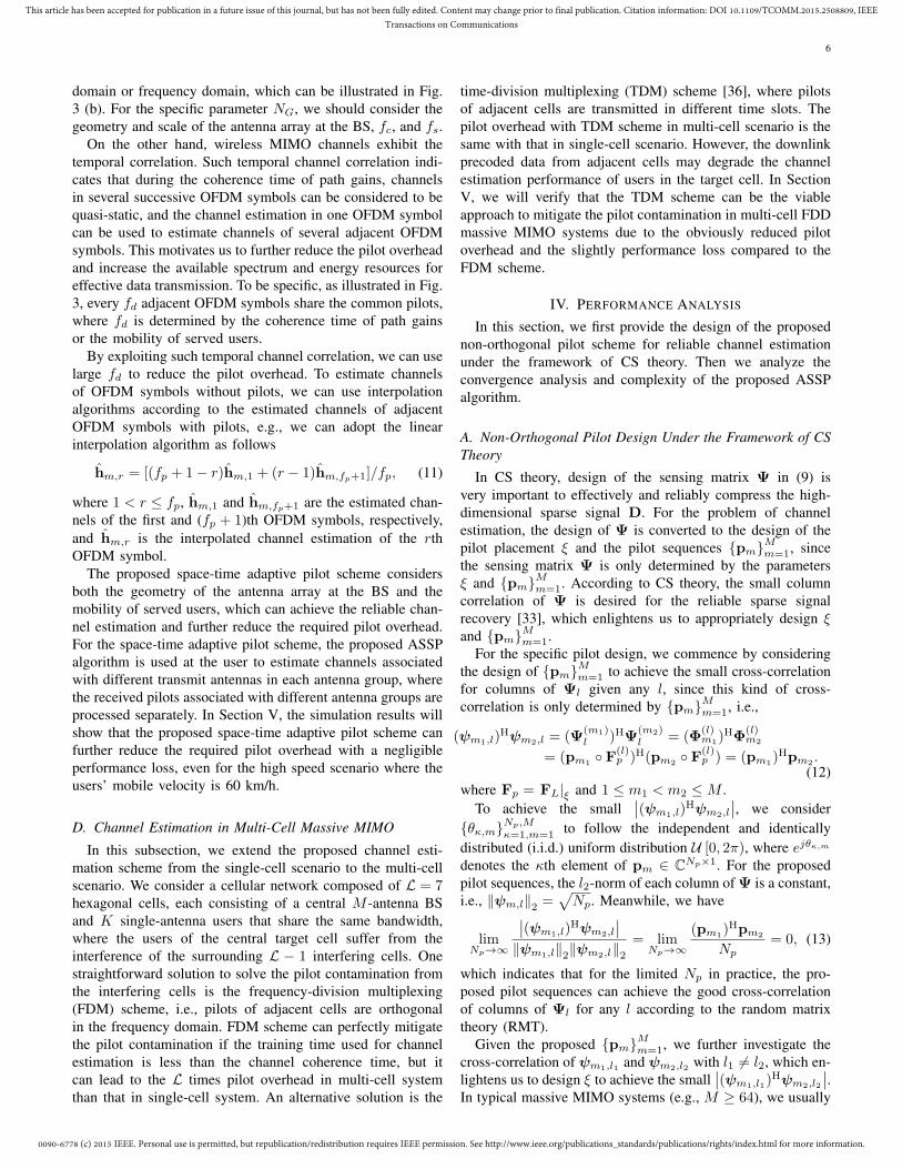
Fig. 5. Estimated channel sparsity level of the proposed ASSP algorithm against SNR and pilot overhead ratio.

10 12 14 16 18 20 22 24 26 28 30

10-3

10-2

10-1

SNR (dB)

MS

E

Proposed, ASSP Algorithm

Random, ASSP Algorithm

Proposed, Oracle LS Algorithm

Random, Oracle LS Algorithm

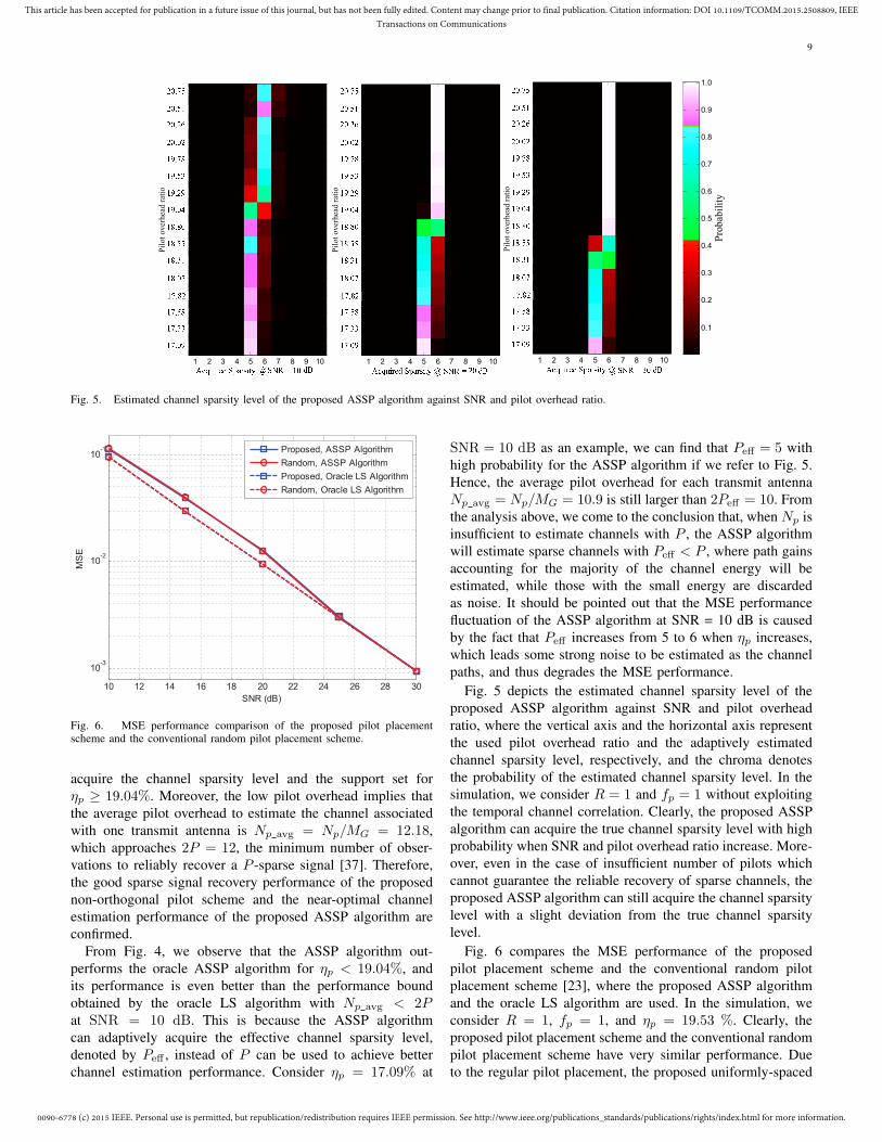
Fig. 6. MSE performance comparison of the proposed pilot placementscheme and the conventional random pilot placement scheme.

acquire the channel sparsity level and the support set forηp ≥ 19.04%. Moreover, the low pilot overhead implies thatthe average pilot overhead to estimate the channel associatedwith one transmit antenna is Np avg = Np/MG = 12.18,which approaches 2P = 12, the minimum number of obser-vations to reliably recover a P -sparse signal [37]. Therefore,the good sparse signal recovery performance of the proposednon-orthogonal pilot scheme and the near-optimal channelestimation performance of the proposed ASSP algorithm areconfirmed.

From Fig. 4, we observe that the ASSP algorithm out-performs the oracle ASSP algorithm for ηp < 19.04%, andits performance is even better than the performance boundobtained by the oracle LS algorithm with Np avg < 2Pat SNR = 10 dB. This is because the ASSP algorithmcan adaptively acquire the effective channel sparsity level,denoted by Peff , instead of P can be used to achieve betterchannel estimation performance. Consider ηp = 17.09% at

SNR = 10 dB as an example, we can find that Peff = 5 withhigh probability for the ASSP algorithm if we refer to Fig. 5.Hence, the average pilot overhead for each transmit antennaNp avg = Np/MG = 10.9 is still larger than 2Peff = 10. Fromthe analysis above, we come to the conclusion that, when Np isinsufficient to estimate channels with P , the ASSP algorithmwill estimate sparse channels with Peff < P , where path gainsaccounting for the majority of the channel energy will beestimated, while those with the small energy are discardedas noise. It should be pointed out that the MSE performancefluctuation of the ASSP algorithm at SNR = 10 dB is causedby the fact that Peff increases from 5 to 6 when ηp increases,which leads some strong noise to be estimated as the channelpaths, and thus degrades the MSE performance.

Fig. 5 depicts the estimated channel sparsity level of theproposed ASSP algorithm against SNR and pilot overheadratio, where the vertical axis and the horizontal axis representthe used pilot overhead ratio and the adaptively estimatedchannel sparsity level, respectively, and the chroma denotesthe probability of the estimated channel sparsity level. In thesimulation, we consider R = 1 and fp = 1 without exploitingthe temporal channel correlation. Clearly, the proposed ASSPalgorithm can acquire the true channel sparsity level with highprobability when SNR and pilot overhead ratio increase. More-over, even in the case of insufficient number of pilots whichcannot guarantee the reliable recovery of sparse channels, theproposed ASSP algorithm can still acquire the channel sparsitylevel with a slight deviation from the true channel sparsitylevel.

Fig. 6 compares the MSE performance of the proposedpilot placement scheme and the conventional random pilotplacement scheme [23], where the proposed ASSP algorithmand the oracle LS algorithm are used. In the simulation, weconsider R = 1, fp = 1, and ηp = 19.53 %. Clearly, theproposed pilot placement scheme and the conventional randompilot placement scheme have very similar performance. Dueto the regular pilot placement, the proposed uniformly-spaced



10

17.1 17.3 17.6 17.8 18.1 18.3 18.6 18.8 19 19.3 19.5 19.8 20 20.3 20.5 20.8

10-3

10-2

10-1


G = 64

MS

E

SSAMP Algorithm, R = 4

Orale LS

SNR = 10 dB

SNR = 20 dB

SNR = 30 dB

Pilot overhead ratio (%)

ASSP Algorithm, R=1ASSP Algorithm, R=4

Oracle LS Algorithm

p

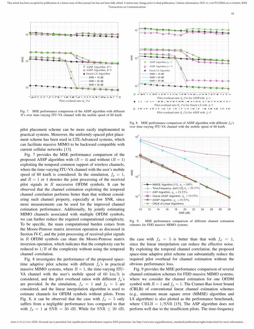
Fig. 7. MSE performance comparison of the ASSP algorithm with differentR’s over time-varying ITU-VA channel with the mobile speed of 60 km/h.

pilot placement scheme can be more easily implemented inpractical systems. Moreover, the uniformly-spaced pilot place-ment scheme has been used in LTE-Advanced systems, whichcan facilitate massive MIMO to be backward compatible withcurrent cellular networks [13].

Fig. 7 provides the MSE performance comparison of theproposed ASSP algorithm with (R = 4) and without (R = 1)exploiting the temporal common support of wireless channels,where the time-varying ITU-VA channel with the user’s mobilespeed of 60 km/h is considered. In the simulation, fp = 1,and R = 1 or 4 denotes the joint processing of the receivedpilot signals in R successive OFDM symbols. It can beobserved that the channel estimation exploiting the temporalchannel correlation performs better than that without consid-ering such channel property, especially at low SNR, sincemore measurements can be used for the improved channelestimation performance. Additionally, by jointly estimatingMIMO channels associated with multiple OFDM symbols,we can further reduce the required computational complexity.To be specific, the main computational burden comes fromthe Moore-Penrose matrix inversion operation as discussed inSection IV-C, and the joint processing of received pilot signalsin R OFDM symbols can share the Moore-Penrose matrixinversion operation, which indicates that the complexity can bereduced to 1/R of the complexity without using the temporalchannel correlation.

Fig. 8 investigates the performance of the proposed space-time adaptive pilot scheme with different fp’s in practicalmassive MIMO systems, where R = 1, the time-varying ITU-VA channel with the user’s mobile speed of 60 km/h isconsidered, and the pilot overhead ratios with different fp’sare provided. In the simulation, fd = 1 and fd = 5 areconsidered, and the linear interpolation algorithm is used toestimate channels for OFDM symbols without pilots. FromFig. 8, it can be observed that the case with fd = 5 onlysuffers from a negligible performance loss compared to thatwith fd = 1 at SNR = 30 dB. While for SNR ≤ 20 dB,

17.1 17.3 17.6 17.8 18.1 18.3 18.6 18.8 19 19.3 19.5 19.8 20 20.3 20.5 20.8

10-3

10-2

10-1


G = 64

MS

E

ASSP Algorithm, fd =1

ASSP Algorithm, fd =5

Orale LS

SNR = 10 dB

SNR = 20 dB

SNR = 30 dB

Pilot overhead ratio (%) for ASSP with fp=5

Pilot overhead ratio (%) for ASSPwith fp=1

ASSP Algorithm, fd = 1

ASSP Algorithm, fd = 5

Oracle LS Algorithm

p

p

Pilot overhead ratio (%) for Oracle LS with fp=1p

Fig. 8. MSE performance comparison of ASSP algorithm with different fd’sover time-varying ITU-VA channel with the mobile speed of 60 km/h.

10 12 14 16 18 20 22 24 26 28 30

10-3

10-2

10-1

100

SNR (dB)

MS

E

MMSE Algorithm [11], xx x

Time-Frequency Joint [15], x

ASP Algorithm,

Oracle ASSP Algorithm,

ASSP Algorithm,

CRLB of Linear Algorithms

20.31%p

!

19.53%p

!

100%p

!

19.53%p

!

19.53%p

!

Fig. 9. MSE performance comparison of different channel estimationschemes for FDD massive MIMO systems.

the case with fd = 5 is better than that with fd = 1,since the linear interpolation can reduce the effective noise.By exploiting the temporal channel correlation, the proposedspace-time adaptive pilot scheme can substantially reduce therequired pilot overhead for channel estimation without theobvious performance loss.

Fig. 9 provides the MSE performance comparison of severalchannel estimation schemes for FDD massive MIMO systems,where we consider the channel estimation for one OFDMsymbol with R = 1 and fp = 1. The Cramer-Rao lower bound(CRLB) of conventional linear channel estimation schemes(e.g., minimum mean square error (MMSE) algorithm andLS algorithm) is also plotted as the performance benchmark,where CRLB = 1/SNR [15]. The ASP algorithm does notperform well due to the insufficient pilots. The time-frequency



11

5 6 7 8 9 10 11 12 13 14 1510

-5

10-4

10-3

10-2

10-1

100

SNR (dB)

MS

E

MMSE Algorithm [11], xx x

Time-Frequency Joint [15], x

ASP Algorithm,

Oracle ASSP Algorithm,

ASSP Algorithm,

20.31%p

!

19.53%p

!

100%p

!

19.53%p

!

19.53%p

!

Fig. 10. BER performance comparison of different channel estimationschemes for FDD massive MIMO systems.

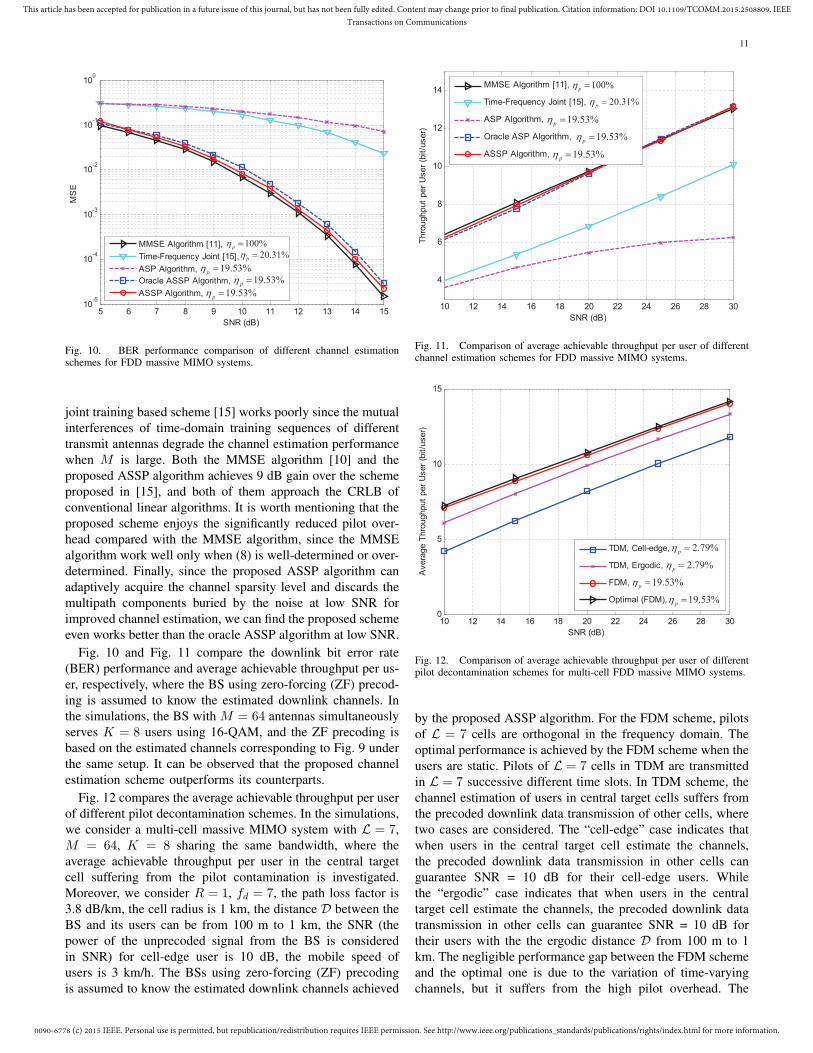
joint training based scheme [15] works poorly since the mutualinterferences of time-domain training sequences of differenttransmit antennas degrade the channel estimation performancewhen M is large. Both the MMSE algorithm [10] and theproposed ASSP algorithm achieves 9 dB gain over the schemeproposed in [15], and both of them approach the CRLB ofconventional linear algorithms. It is worth mentioning that theproposed scheme enjoys the significantly reduced pilot over-head compared with the MMSE algorithm, since the MMSEalgorithm work well only when (8) is well-determined or over-determined. Finally, since the proposed ASSP algorithm canadaptively acquire the channel sparsity level and discards themultipath components buried by the noise at low SNR forimproved channel estimation, we can find the proposed schemeeven works better than the oracle ASSP algorithm at low SNR.

Fig. 10 and Fig. 11 compare the downlink bit error rate(BER) performance and average achievable throughput per us-er, respectively, where the BS using zero-forcing (ZF) precod-ing is assumed to know the estimated downlink channels. Inthe simulations, the BS with M = 64 antennas simultaneouslyserves K = 8 users using 16-QAM, and the ZF precoding isbased on the estimated channels corresponding to Fig. 9 underthe same setup. It can be observed that the proposed channelestimation scheme outperforms its counterparts.

Fig. 12 compares the average achievable throughput per userof different pilot decontamination schemes. In the simulations,we consider a multi-cell massive MIMO system with L = 7,M = 64, K = 8 sharing the same bandwidth, where theaverage achievable throughput per user in the central targetcell suffering from the pilot contamination is investigated.Moreover, we consider R = 1, fd = 7, the path loss factor is3.8 dB/km, the cell radius is 1 km, the distance D between theBS and its users can be from 100 m to 1 km, the SNR (thepower of the unprecoded signal from the BS is consideredin SNR) for cell-edge user is 10 dB, the mobile speed ofusers is 3 km/h. The BSs using zero-forcing (ZF) precodingis assumed to know the estimated downlink channels achieved

10 12 14 16 18 20 22 24 26 28 30

4

6

8

10

12

14

SNR (dB)

Thro

ughput

per

User

(bit/u

ser)

MMSE Algorithm [11], p=100%

Time-Frequency Joint [15], p = 20.31%

ASP Algorithm, p=19.53%

Oracle ASP Algorithm, p=19.53%

ASSP Algorithm, p=19.53%

20.31%p

!

19.53%p

!

100%p

!

19.53%p

!

19.53%p

!

19.53%p

!

Fig. 11. Comparison of average achievable throughput per user of differentchannel estimation schemes for FDD massive MIMO systems.

10 12 14 16 18 20 22 24 26 28 300

5

10

15

SNR (dB)

Avera

ge T

hro

ughput

per

User

(bit/u

ser)

TDM, Cell-edge, p=2.79%

TDM, Ergodic, p=2.79%

FDM, p=19.53%

Optimal (FDM), p=19.53%

2.79%p

!

19.53%p

!

2.79%p

!

19.53%p

!

Fig. 12. Comparison of average achievable throughput per user of differentpilot decontamination schemes for multi-cell FDD massive MIMO systems.

by the proposed ASSP algorithm. For the FDM scheme, pilotsof L = 7 cells are orthogonal in the frequency domain. Theoptimal performance is achieved by the FDM scheme when theusers are static. Pilots of L = 7 cells in TDM are transmittedin L = 7 successive different time slots. In TDM scheme, thechannel estimation of users in central target cells suffers fromthe precoded downlink data transmission of other cells, wheretwo cases are considered. The “cell-edge” case indicates thatwhen users in the central target cell estimate the channels,the precoded downlink data transmission in other cells canguarantee SNR = 10 dB for their cell-edge users. Whilethe “ergodic” case indicates that when users in the centraltarget cell estimate the channels, the precoded downlink datatransmission in other cells can guarantee SNR = 10 dB fortheir users with the the ergodic distance D from 100 m to 1km. The negligible performance gap between the FDM schemeand the optimal one is due to the variation of time-varyingchannels, but it suffers from the high pilot overhead. The



12

TDM scheme with the “cell-edge” case performs worst. Whilethe performance of the TDM scheme with the “ergodic” caseapproaches that of the optimal one. The simulation resultsin Fig. 12 indicates that the TDM scheme with low pilotoverhead can achieve the good performance when dealingthe pilot contamination in multi-cell FDD massive MIMOsystems. Moreover, if some appropriate scheduling strategiesare considered [36], the performance of the TDM scheme canbe further improved.

VI. CONCLUSIONS

In this paper, we have proposed the SCS-based spatio-temporal joint channel estimation scheme for FDD massiveMIMO systems, whereby the intrinsically spatio-temporalcommon sparsity of wireless MIMO channels is exploitedto reduce the pilot overhead. First, the non-orthogonal pilotscheme at the BS and the ASSP algorithm at the user canreliably estimate channels with significantly reduced pilotoverhead. Then, the space-time adaptive pilot scheme canfurther reduce the required pilot overhead according to themobility of users. Moreover, we discuss the proposed channelestimation scheme in multi-cell scenario. Additionally, wediscuss the non-orthogonal pilot design to achieve the reliablechannel estimation under the framework of CS theory, and theconvergence analysis as well as the complexity analysis of theproposed ASSP algorithm are also provided. Simulation resultshave shown that the proposed channel estimation schemecan achieve much better channel estimation performance thanits counterparts with substantially reduced pilot overhead,and it only suffers from a negligible performance loss whencompared with the performance bound.

APPENDIX

A. Proof of Theorem 1

We first provide the definition of SRIP for Ψ in our problemY = ΨD + W (9), where D has the structured sparsity asillustrated in (10). Particularly, the SRIP can be expressed as

√1− δ ∥DΩ∥F ≤ ∥ΨΩDΩ∥F ≤

√1 + δ ∥DΩ∥F , (24)

where δ ∈ [0, 1), Ω is an arbitrary set with |Ω|c ≤ P , andδP is the infimum of all δ satisfying (24). Note that for (24),Ψ = [Ψ1,Ψ2, · · · ,ΨL] ∈ CNp×ML with Ψl ∈ CNp×M for1 ≤ l ≤ L, D = [DT

1 ,DT2 , · · · ,DT

L]T ∈ CML×R with Dl ∈

CM×R for 1 ≤ l ≤ L, ΨΩ =[ΨΩ(1),ΨΩ(2), · · · ,ΨΩ(|Ω|c)

]and DΩ =

[DT

Ω(1),DTΩ(2), · · · ,D

TΩ(|Ω|c)

]T, and Ω(1) <

Ω(2) < · · · < Ω(|Ω|c) are elements in the set Ω. Clearly,for two different sparsity levels P1 and P2 with P1 < P2, wehave δP1 ≤ δP2 . Moreover, for two sets with Ω1 ∩ Ω2 = ϕand the structured sparse matrix D with the support set Ω2,we have∥∥ΨH

Ω1ΨD

∥∥F=

∥∥ΨHΩ1

ΨΩ2DΩ2

∥∥F≤ δ|Ω1|c+|Ω2|c∥D∥F ,

(25)(1−

δ|Ω1|c+|Ω2|c√(1−δ|Ω1|c

)(1−δ|Ω2|c))∥ΨΩ2DΩ2∥F

≤∥∥∥(I−ΨΩ1Ψ

†Ω1

)ΨΩ2DΩ2

∥∥∥F≤ ∥ΨΩ2DΩ2∥F ,

(26)

which will be proven in Appendix B and C, respectively.

To prove (21), we need to investigate the upper bound of∥∥∥D−D∥∥∥F

, which can be expressed as∥∥∥D− D∥∥∥F≤

∥∥∥DΩ −Ψ†ΩY∥∥∥F+

∥∥∥DΩT /Ω

∥∥∥F

=∥∥∥DΩ −Ψ†

Ω(ΨΩT DΩT +W)

∥∥∥F+

∥∥∥DΩT /Ω

∥∥∥F

≤∥∥∥DΩ −Ψ†

ΩΨΩT DΩT

∥∥∥F+

∥∥∥Ψ†ΩW

∥∥∥F+

∥∥∥DΩT /Ω

∥∥∥F

=∥∥∥Ψ†

ΩΨΩT /ΩDΩT /Ω

∥∥∥F+

∥∥∥Ψ†ΩW

∥∥∥F+

∥∥∥DΩT /Ω

∥∥∥F,

(27)where Ω is the estimated support set, ΩT is the correctsupport set, and ΩT /Ω denotes a set whose elements be-long to ΩT except for Ω. The first inequality is due to

∥D∥2F =∥∥DΩ

∥∥2F

+∥∥∥DΩT /Ω

∥∥∥2F

. The second equality isdue to ΨΩT

DΩT= ΨΩT /ΩDΩT /Ω + ΨΩT∩ΩDΩT∩Ω and

DΩ = Ψ†ΩΨΩT∩ΩDΩT∩Ω.

For∥∥∥Ψ†

ΩΨΩT /ΩDΩT /Ω

∥∥∥F

, we have∥∥∥Ψ†ΩΨΩT /ΩDΩT /Ω

∥∥∥F

=∥∥∥(ΨH

ΩΨ

Ω)−1

ΨHΩΨΩT /ΩDΩT /Ω

∥∥∥F≤ δ2P

1−δP

∥∥∥DΩT /Ω

∥∥∥F,

(28)where the inequality of (28) is due to (24) and (25). Similarly,we have

∥∥∥Ψ†ΩW

∥∥∥F≤

√1+δP1−δP

∥W∥F . Thus we have

∥∥∥D− D∥∥∥F≤ 1−δP+δ2P

1−δP

∥∥∥DΩT /Ω

∥∥∥F+

√1+δP

1−δP∥W∥F . (29)

Then we will investigate the relationship between∥∥∥DΩT /Ω

∥∥∥F

and ∥W∥F . It should be pointed out that, after we get Ω, wehave

∥∥Rk−1∥∥F≤

∥∥Rk∥∥F

, which inspires us to first study therelationship between

∥∥Rk∥∥F

and∥∥Rk−1

∥∥F

.For

∥∥Rk∥∥F

, we can obtain∥∥Rk∥∥F=

∥∥∥ΨD+W−ΨΩkΨ†Ωk (ΨD+W)

∥∥∥F

≤∥∥∥(I−ΨΩkΨ

†Ωk)ΨΩT /ΩkDΩT /Ωk

∥∥∥F+∥∥∥W−ΨΩkΨ

†ΩkW

∥∥∥F

≤∥∥∥ΨΩT /ΩkDΩT /Ωk

∥∥∥F+∥W∥F

≤√1+δP

∥∥∥DΩT /Ωk

∥∥∥F+∥W∥F .

(30)where we have ΨD=ΨΩT∩ΩkDΩT∩Ωk+ΨΩT /ΩkDΩT /Ωk ,ΨΩT∩ΩkDΩT∩Ωk=ΨΩkΨ

†Ωk

ΨΩT∩ΩkDΩT∩Ωk , and the sec-

ond inequality is due to (26) and∥∥∥W−ΨΩkΨ

†Ωk

W∥∥∥F

≤∥W∥F .

On the other hand, we consider∥∥Rk−1

∥∥F

, which can beexpressed as∥∥Rk−1

∥∥F≥

∥∥∥(I−ΨΩkΨ†Ωk )ΨΩT /Ωk−1DΩT /Ωk−1

∥∥∥F−∥W∥F

≥ 1−δP−δ2P1−δP

∥∥∥ΨΩT /Ωk−1DΩT /Ωk−1

∥∥∥F−∥W∥F

≥ 1−δP−δ2P√1−δP

∥∥∥DΩT /Ωk−1

∥∥∥F−∥W∥F ,

(31)where the second inequality is due to (26).

To further investigate the relationship between (30) and(31), we will derive the relationship between

∥∥∥DΩT /Ωk

∥∥∥F

and∥∥∥DΩT /Ωk−1

∥∥∥F

. For convenience, we denote Ω∆ =



13

Πs(∥Zl∥F

Ll=1

)in Step 2.3 of Algorithm 1, then we can

get

∥∥ΨHΩ∆

Rk−1∥∥

F=

∥∥∥ΨHΩ∆

(Y −ΨΩk−1Ψ

†Ωk−1Y)

∥∥∥F

=∥∥∥ΨH

Ω∆(ΨD+W −Ψ

Ωk−1Ψ†Ωk−1(ΨD+W))

∥∥∥F

≤∥∥∥ΨH

Ω∆(ΨD−Ψ

Ωk−1Ψ†Ωk−1ΨD)

∥∥∥F

+∥∥∥ΨH

Ω∆(W −Ψ

Ωk−1Ψ†Ωk−1W)

∥∥∥F.

(32)For the first part of the right-hand in the inequality of (32),we denote R′k−1

= ΨD−ΨΩk−1Ψ

†Ωk−1

ΨD, and

R′k−1= (I−Ψ

Ωk−1Ψ†Ωk−1)(ΨΩT /Ωk−1DΩT /Ωk−1

+ΨΩT∩Ωk−1DΩT∩Ωk−1)

= [ΨΩT /Ωk−1 ,ΨΩk−1 ]

[D

ΩT /Ωk−1

−Ψ†Ωk−1ΨΩT /Ωk−1DΩT /Ωk−1

]= ΨΩT∪Ωk−1D

k−1,(33)

where ΨΩT∪Ωk−1 = [Ψ

ΩT /Ωk−1 ,ΨΩk−1 ] and

Dk−1 = [DTΩT /Ωk−1 ,−(Ψ†

Ωk−1ΨΩT /Ωk−1DΩT /Ωk−1)T]T.

The second equality of (33) is due to ΨΩT∩Ωk−1DΩT∩Ωk−1 −Ψ

Ωk−1Ψ†Ωk−1

ΨΩT∩Ωk−1DΩT∩Ωk−1 = 0. It should be pointedout that if W = 0, we have R′k−1

= Rk−1. For the secondpart of the right-hand in the inequality of (32), we have∥∥∥ΨH

Ω∆(W −Ψ


∥∥∥F

=∥∥∥ΨH

Ω∆(I−Ψ

Ωk−1Ψ†Ωk−1)W

∥∥∥F≤

√1 + δP ∥W∥F .

(34)By substituting (33) and (34) into (32), we have

∥∥ΨHΩ∆

Rk−1∥∥

F≤

∥∥∥ΨHΩ∆

ΨΩT∪Ωk−1Dk−1

∥∥∥F+

√1 + δP ∥W∥F

=∥∥∥ΨH

Ω∆R′k−1

∥∥∥F+

√1 + δP ∥W∥F ,

(35)On the other hand, we have∥∥ΨH

Ω∆Rk−1

∥∥F≥∥∥ΨH

ΩTRk−1

∥∥F

≥∥∥∥ΨH

ΩT(ΨD−Ψ

Ωk−1Ψ†Ωk−1ΨD)

∥∥∥F

−∥∥∥ΨH

ΩT(W −Ψ


∥∥∥F

≥∥∥∥ΨH

ΩTR′k−1

∥∥∥F−

√1 + δP ∥W∥F .

(36)Combining (35) and (36), we have∥∥∥ΨH

Ω∆R′k−1

∥∥∥F≥

∥∥∥ΨHΩT

R′k−1∥∥∥F− 2

√1 + δP ∥W∥F . (37)

Due to the following inequality∥∥∥ΨHΩ∆

R′k−1∥∥∥F≥

∥∥∥ΨHΩT

R′k−1

∥∥∥F≥

∥∥∥ΨHΩT /Ωk−1R

′k−1∥∥∥F,

(38)(37) can be further expressed as the following inequality byremoving the common set of Ω∆ and ΩT /Ω

k−1, i.e.,∥∥∥ΨHΩ∆/ΩT

R′k−1

∥∥∥F≥

∥∥∥ΨHΩT /Ωk−1/Ω∆

R′k−1

∥∥∥F− 2

√1 + δP ∥W∥F ,

(39)

here∥∥∥ΨH

ΩT /Ωk−1/Ω∆R

′k−1∥∥∥F

can be expressed as∥∥∥ΨHΩT /Ωk−1/Ω∆

R′k−1

∥∥∥F=

∥∥∥ΨHΩT /Ω

′kR′k−1

∥∥∥F

=∥∥∥ΨH

ΩT /Ω′kΨΩT∪Ωk−1D

k−1∥∥∥F

=∥∥∥ΨH

ΩT /Ω′k (ΨΩT∪Ωk−1/ΩT /Ω

′kDk−1

ΩT∪Ωk−1/ΩT /Ω′k

+ ΨΩT /Ω′kD

k−1

ΩT /Ω′k)

∥∥∥F

≥∥∥∥ΨH

ΩT /Ω′kΨΩT /Ω

′kDk−1

ΩT /Ω′k

∥∥∥F

−∥∥∥ΨH

ΩT /Ω′kΨΩT∪Ωk−1/ΩT /Ω

′kDk−1

ΩT∪Ωk−1/ΩT /Ω′k

∥∥∥F

≥ (1− δP )∥∥∥Dk−1

ΩT /Ω′k

∥∥∥F− δ3P

∥∥∥Dk−1∥∥∥F

= (1− δP )∥∥∥DΩT /Ω

′k

∥∥∥F− δ3P

∥∥∥Dk−1∥∥∥F,

(40)where the first equality is due to Ω∆ ∩ Ωk−1 = ϕ andΩ∆ ∪ Ωk−1 = Ω′k, the second equality is due to (33),and the last equality is due to the definition of Dk−1. S-ince

∥∥∥ΨHΩ∆/ΩT

R′k−1

∥∥∥F

=∥∥∥ΨH

Ω∆/ΩTΨΩT∪Ωk−1Dk−1

∥∥∥F

≤

δ3P

∥∥∥Dk−1∥∥∥F

, by substituting (40) into (39), we have

(1− δP )∥∥∥D

ΩT /Ω′k

∥∥∥F≤ 2δ3P

∥∥∥Dk−1∥∥∥F+ 2

√1 + δP ∥W∥F .

(41)It should be pointed out that for

∥∥∥Dk−1∥∥∥F

, we can further get∥∥∥Dk−1∥∥∥F≤


∥∥∥F+

∥∥∥Ψ†Ωk−1ΨΩT /Ωk−1DΩT /Ωk−1

∥∥∥F

=∥∥∥DΩT /Ωk−1

∥∥∥F

+∥∥∥(ΨH

Ωk−1ΨΩk−1)−1

ΨHΩk−1ΨΩT /Ωk−1DΩT /Ωk−1

∥∥∥F

≤∥∥∥DΩT /Ωk−1

∥∥∥F+ δ2P

1−δP


∥∥∥F

= 1−δP+δ2P1−δP


∥∥∥F,

(42)where the first inequality is due to the definition of Dk−1. Bysubstituting (41) into (42), we have∥∥∥DΩT /Ωk−1

∥∥∥F≥ (1−δP )2

2δ3P (1−δP+δ2P )

∥∥∥DΩT /Ω′k

∥∥∥F

−√

1+δP (1−δP )

δ3P (1−δP+δ2P )∥W∥F .

(43)

Then, we investigate DΩT /Ωk , which can be expressed as∥∥∥DΩT /Ωk

∥∥∥F=

∥∥∥DΩT∩Ω′k/Ωk+ΩT /Ω′k

∥∥∥F

≤∥∥∥DΩT∩Ω′k/Ωk

∥∥∥F+


∥∥∥F

=∥∥∥DΩ

′k/Ωk

∥∥∥F+


∥∥∥F,

(44)

where we use the fact that Ωk ⊂ Ω′k. For

∥∥∥DΩ′k/Ωk

∥∥∥F

, wecan further obtain∥∥∥DΩ

′k/Ωk

∥∥∥F=

∥∥∥

DΩ′k∩Ω′k/Ωk +E

Ω′k/Ωk

∥∥∥F

≤∥∥∥

DΩ′k∩Ω′k/Ωk

∥∥∥F+

∥∥∥EΩ′k/Ωk

∥∥∥F

≤∥∥∥

DΩ′k∩Ω′

∥∥∥F+


∥∥∥F

=∥∥DΩ

′k∩Ω′ −EΩ′

∥∥F+


∥∥∥F

≤ ∥DΩ′∥F + ∥EΩ′∥F +∥∥∥EΩ

′k/Ωk

∥∥∥F

= 0+ ∥EΩ′∥F +∥∥∥EΩ

′k/Ωk

∥∥∥F

≤ 2∥E∥F ,

(45)



14

where we introduce the error variable E = DΩ′k−

DΩ′k (

DΩ′k

is obtained in Step 2.3 of Algorithm 1), and Ω′ is an arbitraryset satisfying |Ω′|c = P , Ω′ ⊂ Ω

′k, and Ω′ ∩ ΩT = ϕ. Thesecond inequality in (45) is due to the fact that Ω

′k/Ωk is thediscarded support in the step of support pruning in Algorithm1. According to the definition of E, we further obtain

∥E∥F =∥∥∥DΩ

′k −

DΩ′k

∥∥∥F=∥∥∥DΩ

′k −Ψ†Ω

′kY∥∥∥F

=∥∥∥DΩ

′k −Ψ†Ω

′k(ΨD+W)∥∥∥F

≤∥∥∥DΩ

′k −Ψ†Ω

′kΨD∥∥∥F+∥∥∥Ψ†

Ω′kW

∥∥∥F

=∥∥∥DΩ

′k −Ψ†Ω

′kΨΩT DΩT

∥∥∥F+∥∥∥Ψ†

Ω′kW

∥∥∥F.

(46)

For∥∥∥DΩ′k −Ψ†

Ω′kΨΩTDΩT

∥∥∥F

, we can have∥∥∥DΩ′k −Ψ†

Ω′kΨΩT DΩT

∥∥∥F

=∥∥∥DΩ

′k −Ψ†Ω

′k(ΨΩT∩Ω′kDΩT∩Ω

′k +ΨΩT /Ω′kDΩT /Ω

′k)∥∥∥F

=∥∥∥(DΩ

′k−Ψ†Ω

′kΨΩT∩Ω′kDΩT∩Ω

′k)−Ψ†Ω

′kΨΩT /Ω′kDΩT /Ω

′k

∥∥∥F

=∥∥∥(DΩ

′k −Ψ†Ω

′kΨΩ′kDΩ

′k)−Ψ†Ω

′kΨΩT /Ω′kDΩT /Ω

′k

∥∥∥F

=∥∥∥DΩ

′k −DΩ′k −Ψ†

Ω′kΨΩT /Ω

′kDΩT /Ω′k

∥∥∥F

=∥∥∥Ψ†

Ω′kΨΩT /Ω

′kDΩT /Ω′k

∥∥∥F

≤ δ3P1−δ2P


∥∥∥F,

(47)where the last inequality is due to |Ω′k|c = 2P . While for∥∥∥Ψ†

Ω′kW∥∥∥F

in (46), we have∥∥∥Ψ†Ω′kW

∥∥∥F≤ δ2P /

√1−δ2P ∥W∥F . (48)

By substituting (45)-(48) into (44), we can obtain


∥∥∥F≥

(1−δ2P )∥∥∥DΩT /Ωk

∥∥∥F− 2δP

√1−δ2P ∥W∥F

1−δ2P + 2δ3P.

(49)Furthermore, by substituting (49) into (43), we can obtain∥∥∥DΩT /Ωk−1

∥∥∥F≥ (1− δP )

2(1− δ2P )

2δ3P (1− δP + δ2P )(1− δ2P + δ3P )︸︷︷︸C1

∥∥∥DΩT /Ωk

∥∥∥F

− (1− δP )

δ3P (1− δP + δ2P )(δP (1− δP )

√1− δ2P

(1− δ2P + 2δ3P )+

√1 + δP )︸︷︷︸

C2

∥W∥F .

(50)As we have discussed, if

∥∥Rk−1∥∥F

≤∥∥Rk

∥∥F

, the iterationquits, which indicates that the estimation of the P -sparsesignal D is obtained, and Ω = Ωk−1. Then we can combine(30), (31), and (50) to obtain∥∥∥DΩT /Ω

∥∥∥F≤ C3∥W∥F , (51)

where C3 =2C1

√1−δP+C2

√1−δ2P

C1(1−δP−δ2P )−√

1−δ2P. By substituting (29) into

(51), we have ∥∥∥D− D∥∥∥F≤ C4∥W∥F , (52)

where C4 =C3(1−δP+δ2P )+

√1+δP

1−δP. Thus we prove (21).

Finally, in the iterative process, we have∥∥Rk−1

∥∥F>

∥∥Rk∥∥F

,

and by substituting (30) and (31) into (50), we can obtain∥∥Rk−1∥∥F> C1(1−δP−δ2P )√

1−δ2P

∥∥Rk∥∥F

− (1 +(1−δP−δ2P )(C1+C2

√1+δ

P)√

1−δ2P

)∥W∥F .(53)

In this way, we prove (22).B. Proof of (25)

We consider two matrices D′ and D have the structuredsparsity as illustrated in (10), and both of them have the re-spective structured support set Ω1 and Ω1, where Ω1∩Ω2 = ϕ.Moreover, we consider D′ = D′/∥D′∥F and D = D/∥D∥F .According to (24), we can obtain

2(1− δ|Ω1|c+|Ω2|c) ≤∥∥∥∥[ΨΩ1 ,ΨΩ2 ]

[D′

Ω1

DΩ2

]∥∥∥∥2

F

≤ 2(1 + δ|Ω1|c+|Ω2|c),

(54)

2(1− δ|Ω1|c+|Ω2|c) ≤∥∥∥∥[ΨΩ1 ,ΨΩ2]

[D′

Ω1

−DΩ2

]∥∥∥∥2

F

≤2(1 + δ|Ω1|c+|Ω2|c).

(55)From (54) and (55), we obtain

−δ|Ω1|c+|Ω2|c ≤ Re⟨ΨΩ1D

′Ω1

,ΨΩ2DΩ2

⟩ ≤ δ|Ω1|c+|Ω2|c ,

(56)where for two matrices A and B, we have Re ⟨A,B⟩ =∥A+B∥2

F−∥A−B∥2F

4 . Moreover, we exploit the Cauchy-Schwartz inequality ∥A∥F ∥B∥F ≥ |⟨A,B⟩|, where the e-quality holds only for A = cB and c is a complex constant.Particularly,∥∥∥D′

Ω1

∥∥∥F

∥∥ΨHΩ1

ΨΩ2DΩ2

∥∥F

= maxD

′Ω1

=c′ΨHΩ1

ΨΩ2DΩ2

∣∣∣⟨ΨΩ1D′Ω1

,ΨΩ2DΩ2

⟩∣∣∣= max

D′Ω1

=c′ΨHΩ1

ΨΩ2DΩ2

(∣∣∣Re

⟨ΨΩ1D

′Ω1

,ΨΩ2DΩ2

⟩∣∣∣)

≤ δ|Ω1|c+|Ω2|c ,

(57)

where c′ is a complex constant, and the second e-quality of (57) is due to Im

⟨ΨΩ1D

′Ω1

,ΨΩ2DΩ2

⟩ =

c′Im⟨ΨH

Ω1ΨΩ2DΩ2 ,Ψ

HΩ1

ΨΩ2DΩ2

⟩=0. In this way, we

have ∥∥ΨHΩ1

ΨΩ2DΩ2

∥∥F≤ δ|Ω1|c+|Ω2|c∥DΩ2∥F , (58)

and (25) is proven.C. Proof of (26)

Clearly, we have∥∥∥(I−ΨΩ1Ψ†Ω1

)ΨΩ2DΩ2

∥∥∥F≥∥ΨΩ2DΩ2∥F−

∥∥∥ΨΩ1Ψ†Ω1

ΨΩ2DΩ2

∥∥∥F,

(59)

For∥∥∥ΨΩ1Ψ

†Ω1

ΨΩ2DΩ2

∥∥∥2F

, we have∥∥∥ΨΩ1Ψ†Ω1

ΨΩ2DΩ2

∥∥∥2

F=⟨ΨΩ1Ψ

†Ω1

ΨΩ2DΩ2 ,ΨΩ1Ψ†Ω1

ΨΩ2DΩ2

⟩= Re

⟨ΨΩ1Ψ

†Ω1


ΨΩ2DΩ2

⟩

= Re⟨ΨΩ1Ψ

†Ω1


ΨΩ2DΩ2

+ΨΩ2DΩ2−ΨΩ1Ψ†Ω1

ΨΩ2DΩ2

⟩

= Re⟨ΨΩ1Ψ

†Ω1

ΨΩ2DΩ2 ,ΨΩ2DΩ2

⟩

≤ δ|Ω1|c+|Ω2|c

∥∥∥Ψ†Ω1

ΨΩ2DΩ2

∥∥∥F∥DΩ2∥F

≤ δ|Ω1|c+|Ω2|c

∥∥∥ΨΩ1Ψ

†Ω1

ΨΩ2DΩ2

∥∥∥F√

1−δ|Ω1|c

∥ΨΩ2DΩ2∥F√

1−δ|Ω2|c,

(60)



15

where the first inequality in (60) is due to (56), and the thirdequality in (60) is due to the following equality,⟨

ΨΩ1Ψ†Ω1

ΨΩ2DΩ2 ,ΨΩ2DΩ2−ΨΩ1Ψ†Ω1

ΨΩ2DΩ2

⟩=DH

Ω2ΨH

Ω2(Ψ†

Ω1)H(ΨH

Ω1ΨΩ2DΩ2−ΨH

Ω1ΨΩ1Ψ

†Ω1

ΨΩ2DΩ2)

=DHΩ2

ΨHΩ2

(Ψ†Ω1

)H(ΨHΩ1

ΨΩ2DΩ2−ΨHΩ1

ΨΩ2DΩ2)=0.(61)

Here Ψ†Ω1

= (ΨHΩ1

ΨΩ1)−1

ΨHΩ1

. Moreover, (60) can be ex-pressed as∥∥∥ΨΩ1Ψ

†Ω1

ΨΩ2DΩ2

∥∥∥F≤

δ|Ω1|c+|Ω2|c∥ΨΩ2DΩ2∥F√(1− δ|Ω1|c)(1− δ|Ω2|c)

. (62)

By substituting (62) into (59), we have∥∥∥(I−ΨΩ1Ψ†Ω1

)ΨΩ2DΩ2

∥∥∥F≥(1−

δ|Ω1|c+|Ω2|c√(1−δ|Ω1|c

)(1−δ|Ω2|c))∥ΨΩ2DΩ2∥F ,

(63)Thus, the right inequality of (26) is proven. Finally, due to(61), we have

∥ΨΩ2DΩ2∥2F=

∥∥∥ΨΩ1Ψ†Ω1

ΨΩ2DΩ2

∥∥∥2

F+∥∥∥(I−ΨΩ1Ψ

†Ω1

)ΨΩ2DΩ2

∥∥∥2

F,

(64)which indicates

∥ΨΩ2DΩ2∥F ≥∥∥∥(I−ΨΩ1Ψ

†Ω1

)ΨΩ2DΩ2

∥∥∥F. (65)

Hence the left inequality of (26) is proven.

REFERENCES

[1] E. G. Larsson, F. Tufvesson, O. Edfors, and T. L. Marzetta, “MassiveMIMO for next generation wireless systems,” IEEE Commun. Mag., vol.52, no. 2, pp. 186-195, Feb. 2014.

[2] L. Lu, G. Y. Li, A. L. Swindlehurst, A. Ashikhmin, and R. Zhang,“An overview of massive MIMO: Benefits and challenges,” IEEE J. Sel.Topics Signal Process., vol. 8, no. 5, pp. 742-758, Oct. 2014.

[3] F. Rusek, D. Persson, B. K. Lau, E. G. Larsson, T. L. Marzetta,O. Edfors, and F. Tufvesson, “Scaling up MIMO: Opportunities andchallenges with very large arrays,” IEEE Signal Process. Mag., vol. 30,no. 1, pp. 40-60, Jan. 2013.

[4] J. Zhang, B. Zhang, S. Chen, X. Mu, M. El-Hajjar, and L. Hanzo, “Pilotcontamination elimination for large-scale multiple-antenna aided OFDMsystems,” IEEE J. Sel. Topics Signal Process., vol. 8, no. 5, pp. 759-772,Oct. 2014.

[5] E. Bjonson, J. Hoydis, M. Kountouris, and M. Debbah, “Massive MIMOsystems with non-ideal hardware: Energy efficiency, estimation, andcapacity limits,” IEEE Trans. Inf. Theory, vol. 60, no. 11, pp. 7112-7139, Nov. 2014.

[6] Y. Cho, J. Kim, W. Yang, and C. Kang, MIMO-OFDM WirelessCommunications with MATLAB, John Wiley & Sons (Asia) Pte Ltd.2010.

[7] Y. Xu, G. Yue, and S. Mao, “User grouping for massive MIMO in FDDsystems: New design methods and analysis,” IEEE Access, vol. 2, pp.947-959, Sep. 2014.

[8] B. Hassibi and B. Hochwald, “How much training is needed in multiple-antenna wireless links?,” IEEE Trans. Inf. Theory, vol. 49, no. 4, pp.951-963, Apr. 2003.

[9] E. Bjonson and B. Ottersten, “A framework for training-based estimationin arbitrarily correlated Rician MIMO channels with Rician distrubance,”IEEE Trans. Signal Process., vol. 58, no. 3, pp. 1807-820, Mar. 2010.

[10] I. Barhumi, G. Leus, and M. Moonen, “Optimal training design forMIMO OFDM systems in mobile wireless channels,” IEEE Trans. SignalProcess., vol. 51, no. 6, pp. 1615-1624, Jun. 2003.

[11] H. Minn and N. Dhahir, “Optimal training signals for MIMO OFDMchannel estimation,” IEEE Trans. Wireless Commun., vol. 5, no. 5, pp.1158-1168, May 2006.

[12] 3GPP Technical Specification 36.211. Evolved Universal Terrestri-al Radio Access (E-UTRA); Physical Channels and Modulation.www.3gpp.org.

[13] Y. Nam, Y. Akimoto, Y. Kim, M. Lee, K. Bhattad, and A. Ekpeny-ong, “Evolution of reference signals for LTE-advanced systems,” IEEECommun. Mag., vol. 50, no. 2, pp. 132-138, Feb. 2012.

[14] L. Correia, Mobile Broadband Multimedia Networks, Techniques, Mod-els and Tools for 4G, San Diego, CA: Academic, 2006.

[15] L. Dai, Z. Wang, and Z. Yang “Spectrally efficient time-frequencytraining OFDM for mobile large-scale MIMO systems,” IEEE J. Sel.Areas Commun., vol. 31, no. 2, pp. 251-263, Feb. 2013.

[16] Z. Gao, L. Dai, and Z. Wang, “Structured compressive sensing basedsuperimposed pilot design for large-scale MIMO systems,” Electron.Lett., vol. 50, no. 12 pp. 896-898, Jun. 2014.

[17] C. Qi and L. Wu, “Uplink channel estimation for massive MIMOsystems exploring joint channel sparsity,” Electron. Lett., vol. 50, no.23, pp.1770-1772, Nov. 2014.

[18] Z. Gao, L. Dai, Z. Lu, C. Yuen, and Z. Wang, “Super-resolutionsparse MIMO-OFDM channel estimation based on spatial and temporalcorrelations,” IEEE Commun. Lett., vol. 18, no. 7, pp. 1266-1269, Jul.2014.

[19] S. L. H. Nguyen and A. Ghrayeb, “Compressive sensing-based channelestimation for massive multiuser MIMO systems,” in Proc. IEEE Wire-less Communications and Networking Conference (IEEE WCNC’13),Shanghai, China, Apr. 2013.

[20] Z. Gao, L. Dai, Z. Wang, and S. Chen, “Spatially common sparsity basedadaptive channel estimation and feedback for FDD massive MIMO,”IEEE Trans. Signal Process., vol. 63, no. 23, pp. 6169-6183, Dec. 2015.

[21] W. Shen, L. Dai, B. Shim, S. Mumtaz, and Z. Wang, “Joint CSITacquisition based on low-rank matrix completion for FDD massiveMIMO systems,” IEEE Commun. Lett., vol. 19, no. 12, pp. 2178-2181,Dec. 2015.

[22] J. Choi, D. J. Love, and P. Bidigare, “Downlink training techniques forFDD massive MIMO systems: Open-loop and closed-loop training withmemory,” IEEE J. Sel. Topics Signal Process., vol. 8, no. 5, pp. 802–814,Oct. 2014.

[23] W. U. Bajwa, J. Haupt, A. M. Sayeed, and R. Nowak, “Compressedchannel sensing: A new approach to estimating sparse multipath chan-nels,” Proc. IEEE, vol. 98, no. 6, pp. 1058-1076, Jun. 2010.

[24] C. R. Berger, Z. Wang, J. Huang, and S. Zhou, “Application of com-pressive sensing to sparse channel estimation,” IEEE Commun. Mag.,vol. 48, no. 11, pp. 164-174, Nov. 2010.

[25] Z. Gao, L. Dai, Z. Wang, and S. Chen, “Priori-information aided iterativehard threshold: A low-complexity high-accuracy compressive sensingbased channel estimation for TDS-OFDM,” IEEE Trans. Wireless Com-mun., vol. 14, no. 1, pp. 242-251, Jan. 2015.

[26] G. Gui and F. Adachi, “Stable adaptive sparse filtering algorithms forestimating multiple-input multiple-output channels,” IET Commun., vol.8, no. 7, pp. 1032-1040, May 2014.

[27] Z. Gao, L. Dai, C. Yuen, and Z. Wang, “Asymptotic orthogonality anal-ysis of time-domain sparse massive MIMO channels,” IEEE Commun.Lett., vol. 19, no. 10, pp. 1826-1829, Oct. 2015.

[28] C. R. Berger, S. Zhou, J. C. Preisig, and P. Willett, “Sparse channelestimation for multicarrier underwater acoustic communication: Fromsubspace methods to compressed sensing,” IEEE Trans. Signal Process.,vol. 58, no. 3, pp. 1708-1721, Mar. 2010.

[29] D. Hu, X. Wang, and L. He, “A new sparse channel estimation andtracking method for time-varying OFDM systems,” IEEE Trans. Veh.Technol., vol. 62, no. 9, pp. 4648-4653, Nov. 2013.

[30] T. Santos, J. Kredal, P. Almers, F. Tufvesson, and A. Molisch, “Mod-eling the ultra-wideband outdoor channel: Measurements and parameterextraction method,” IEEE Trans. Wireless. Commun., vol. 9, no. 1, pp.282-290, Jan. 2010.

[31] I. E. Telatar and D. N. C. Tse, “Capacity and mutual information ofwideband multipath fading channels,” IEEE Trans. Inf. Theory, vol. 46,no. 4, pp. 1384–1400, July 2000.

[32] F. Wan, W. P. Zhu, and M. N. S. Swamy, “Semi-blind most significanttap detection for sparse channel estimation of OFDM systems,” IEEETrans. Circuits and Systems, Part I, vol. 57, no. 3, pp. 703–713, Mar.2010.

[33] M. Duarte and Y. Eldar, “Structured compressed sensing: From theoryto applications,” IEEE Trans. Signal Process., vol. 59, no. 9, pp. 4053–4085, Sep. 2009.

[34] W. Dai and O. Milenkovic, “Subspace pursuit for compressive sensingsignal reconstruction,” IEEE Trans. Inf. Theory, vol. 55, no. 5, pp. 2230-2249, May 2009.

[35] R. G. Baraniuk, V. Cevher, M. F. Duarte, and C. Hegde, “Model-basedcompressive sensing,” IEEE Trans. Inf. Theory, vol. 56, no. 4, pp. 1982-2001, Apr. 2010.



16

[36] F. Fernandes, A. Ashikhmin, and T. L. Marzetta, “Inter-cell interferencein noncooperative TDD large scale antenna systems,” IEEE J. Sel. AreasCommun., vol. 31, no. 2, pp. 192-201, Feb. 2013.

[37] D. L. Donoho and M. Elad, “Optimally sparse representation in general(nonorthogonal) dictionaries via minimization,” Proc. Nat. Acad. Sci.,vol. 100, no. 5, pp. 2197-2202, Mar. 2003.

[38] X. Gao, L. Dai, Y. Hu, Y. Zhang, and Z. Wang, “Low-complexity signaldetection for large-scale MIMO in optical wireless communications,”IEEE J. Sel. Areas. Commun., vol. 33, no. 9, pp. 1903-1912, Sep. 2015.

[39] T. Cormen, C. Lesierson, L. Rivest, and C. Stein, Introduction toAlgorithms, Second ed., MIU Press, Cambridge, MA, 2001.

[40] A. Bjorck, Numerical Methods for Matrix Computations. SpringerInternational Publishing AG, 2014.

[41] L. Dai, X. Gao, X. Su, S. Han, C.-L. I, and Z. Wang, “Low-complexitysoft-output signal detection based on Gauss-Seidel method for uplinkmulti-user large-scale MIMO systems,” IEEE Trans. Veh. Technol., vol.64, no. 10, pp. 4839-4845, Oct. 2015.

Zhen Gao (S’14) received the B.S. degree (with thehighest honor) from Beijing Institute of Technology,Beijing, China, in 2011. He is currently workingtowards Ph. D. degree in Electronic Engineeringof Tsinghua University, Beijing, China. He has au-thored or coauthored over 20 journal and conferencepapers. His research interests are in wireless commu-nications, with a focus on multi-carrier modulations,multiple antenna systems, sparse signal processing.Mr. Gao received the National PhD Scholarshipin 2015, the First-Class Scholarship for Academic

Excellence of Tsinghua University in 2014. He currently serves as asTechnical Program Committee Member of IEEE Wireless Communicationsand Networking Conference (WCNC) 2016.

Linglong Dai (M’11CSM’14) received the B.S.degree from Zhejiang University in 2003, the M.S.degree (with the highest honor) from the China A-cademy of Telecommunications Technology (CATT)in 2006, and the Ph.D. degree (with the highesthonor) from Tsinghua University, Beijing, China, in2011. From 2011 to 2013, he was a postdoctoralfellow with the Department of Electronic Engineer-ing, Tsinghua University, where he has been anassistant professor since July 2013. His researchinterests are in wireless communications, with a

focus on multi-carrier techniques, multi-antenna techniques, and multi-usertechniques. He has published over 50 IEEE journal papers and over 30IEEE conference papers. He has received the Outstanding Ph.D. Graduateof Tsinghua University Award in 2011, the Excellent Doctoral Dissertation ofBeijing Award in 2012, the IEEE ICC Best Paper Award in 2013, the NationalExcellent Doctoral Dissertation Nomination Award in 2013, the IEEE ICCBest Paper Award in 2014, the URSI Young Scientists Award in 2014, theIEEE Transactions on Broadcasting Best Paper Award in 2015, the IEEERADIO Young Scientists Award in 2015. He currently serves as a co-chairof the IEEE Special Interest Group (SIG) on Signal Processing Techniquesin 5G Communication Systems.

Wei Dai (S’01-M’11) is currently a Lecturer in Elec-trical and Electronic Engineering at Imperial CollegeLondon. He received his Ph.D. degree in Electricaland Computer Engineering from the University ofColorado at Boulder in 2007. From 2007 to 2010,he was a Postdoctoral Research Associate in theDepartment of Electrical and Computer Engineering,University of Illinois at Urbana-Champaign.

Byonghyo Shim (SM’09) received the B.S. and M.S.degrees in control and instrumentation engineeringfrom Seoul National University, Korea, in 1995 and1997, respectively. He received the M.S. degree inmathematics and the Ph.D. degree in electrical andcomputer engineering from the University of Illinoisat Urbana-Champaign (UIUC), USA, in 2004 and2005, respectively.From 1997 and 2000, he was with the Department ofElectronics Engineering, Korean Air Force Academyas an Officer (First Lieutenant) and an Academic

Full-time Instructor. From 2005 to 2007, he was with Qualcomm Inc., SanDiego, CA, USA, as a Staff Engineer. From 2007 to 2014, he was with theSchool of Information and Communication, Korea University, Seoul, as anAssociate Professor. Since September 2014, he has been with the Departmentof Electrical and Computer Engineering, Seoul National University, where heis presently an Associate Professor. His research interests include wirelesscommunications, statistical signal processing, estimation and detection, com-pressive sensing, and information theory.Dr. Shim was the recipient of the 2005 M. E. Van Valkenburg Research Awardfrom the Electrical and Computer Engineering Department of the Universityof Illinois and 2010 Hadong Young Engineer Award from IEIE. He is currentlyan Associate Editor of the IEEE Wireless Communications Letters, Journalof Communications and Networks, and a Guest Editor of the IEEE Journalon Selected Areas in Communications (JSAC).

Zhaocheng Wang (M’09-SM’11) received his B.S.,M.S. and Ph.D. degrees from Tsinghua University,Beijing, China, in 1991, 1993, and 1996, respective-ly.From 1996 to 1997, he was a Postdoctoral Fellowwith Nanyang Technological University, Singapore.From 1997 to 1999, he was with OKI Techno Centre(Singapore) Pte. Ltd., Singapore, where he was firsta Research Engineer and later became a SeniorEngineer. From 1999 to 2009, he was with SonyDeutschland GmbH, where he was first a Senior En-

gineer and later became a Principal Engineer. He is currently a Professor withthe Department of Electronic Engineering, Tsinghua University and serves asthe Director of Broadband Communication Key Laboratory, Tsinghua NationalLaboratory for Information Science and Technology (TNlist). He has authoredor coauthored around 90 journal papers (SCI indexed). He is the holder of 34granted U.S./EU patents. He co-authored two books, one of them with the titleof “Millimeter Wave Communication Systems”, was selected by IEEE Serieson Digital & Mobile Communication and published by Wiley-IEEE Press. Hisresearch areas include wireless communications, visible light communications,millimeter-wave communications, and digital broadcasting.Professor Wang is a Fellow of the Institution of Engineering and Technology.Currently he serves as an Associate Editor of IEEE Transactions on WirelessCommunications and an Associate Editor of IEEE Communications Letters,and has also served as Technical Program Committee Co-chairs of variousinternational conferences.

Documents

Zhen Gao, Linglong Dai, Wei Dai, Byonghyo Shim, and ... massive MIMO systems, an accurate acquisition of the channel state information (CSI) is essential for signal detection, beamforming,