Embed Size (px)
DESCRIPTION
raza,
Citation preview
Study of Classical Integrable Field Thoery and Defect Problem
2nd Year Master Research Project in Fundamental PhysicsEcole Normale Superieure de Lyon & Universite Claude Bernard Lyon 1
Cheng [email protected]
Supervised by
Vincent CaudrelierCentre for Mathematical Science
City University, [email protected]
August 20, 2010
This research project is focusing on the study of classical integrable field mod-els and the associated defect problems. I will present a basic understanding ofthese topics. The emphasis of this report will be put on the Inverse ScatteringMethod (ISM). The ISM consists in solving exactly the initial value problemof integrable nonlinear evolution equations by using an auxiliary linear dif-ferential system. It can be considered either as a Fourier-type transform tosolve nonlinear evolution equations or as a canonical transformation in thesense of integrable Hamiltonian system of infinite degrees of freedom. TheLax pair and the AKNS scheme are the generalised auxiliary linear differ-ential systems, used to identify and solve nonlinear equations. Among theinteresting integrable models, the nonlinear Schrodinger equation (NLS) willbe studied in details. In the context of the classical integrable field theories,boundary conditions of fields determine the integrability of systems. An in-ternal boundary condition could be interpreted as a defect. An ISM approachto systematically generate defects in keeping systems completely integrablewill be presented. The modified physical quantities can be identified in termsof defect matrices.
1
Contents
1 Introduction 3
2 Inverse Scattering Method 42.1 Lax Pair . . . . . . . . . . . . . . . . . . . . . . . . . . . . . . . . . . . . . . 42.2 AKNS Scheme . . . . . . . . . . . . . . . . . . . . . . . . . . . . . . . . . . 52.3 Inverse Scattering Method . . . . . . . . . . . . . . . . . . . . . . . . . . . . 82.4 Conservation Laws and Complete Integrability . . . . . . . . . . . . . . . . 12
3 Exact Solution of Nonlinear Schrodinger Equation 163.1 Soliton Solution . . . . . . . . . . . . . . . . . . . . . . . . . . . . . . . . . . 163.2 General Solution of ISM . . . . . . . . . . . . . . . . . . . . . . . . . . . . . 17
4 Defect Problem 19
5 Conclusions and Outlook 21
Appendices 22
A KdV Hierarchy 22
B Proof of Analyticity of φiζx 23
C Symmetry Relations between q and r 25
D Proof of Expression of log a 25
E Proof of No Zeros of a for (σ > 0) in (3.1) 26
Bibliography 27
1 Introduction
The invention of the Inverse Scattering Method (ISM), which marked the birth of theintegrable field theory, was one of the most important advances in mathematical physicsin the 2nd half of 20th century. It was first introduced by Gardner, Greene, Kruskal andMiura [7] to solve the Korteweg-de Vries equation [13] (KdV)
ut + 6uux + uxxx = 0, 1 (1)
which appeared originally in fluid dynamics. They considered a 1D Schrodinger equation
−d2ψ
dx2+ u(x, t)ψ = k2ψ, (2)
whose potential u(x, t) plays the role of the solution of the KdV equation and showed thatexact solution can be obtained by use of the solution of the inverse scattering problemfor the Schrodinger equation. This method was soon expressed in a general form by Lax[14], who introduced the Lax pair to generate a class of integrable nonlinear evolutionequations. In 1972, Zakharov and Shabat [23] solved the nonlinear Schrodinger equation(NLS)
iut + uxx ± 2|u|2u = 0, (3)
by using a 2× 2 Dirac-type operator
∂xξ = −iλξ + u(x, t)η, (4a)∂xη = iλη ± u∗(x, t)ξ. (4b)
In the same year, Wadati [21] showed that the modified Kortewege-de Vries equation(mKdV)
ut + 6u2ux + uxxx = 0, (5)
can be solved by generalising the Zakharov-Shabat system. Soon afterwards in 1973,Ablowitz, Kaup, Newell and Segur [1] showed that the sine-Gordon equation
uxt = sinu, (6)
can be solved in the same way, and they established a general framework [16, 17], nowcalled the AKNS scheme, which identifies and generates nonlinear evolution equationssolvable by the ISM.
In contrast to integrable models of finite degrees of freedom in the sense of Liouville[19, 2]2, the physical quantity u(x, t) in the above equations is a field, and the connectionbetween the ISM to the solve the nonlinear field equations and the integrability of Hamilto-nian systems of infinite degrees of freedom was unveiled by Gardner [8] and Zakharov andFaddeev [22]. This deep insight led soon to an enormous amount of results, and extendedthe topic to quantum mechanics.
The solutions of the above classical integrable models were all first solved under theboundary conditions where the field u(x, t) is defined on an infinite line i.e. −∞ < x <∞,and tends to 0 as |x| → ∞. Since a physical system can not be of infinite size, people
1The subscripts t and x denote partial derivatives with respect to t and x respectively. We will keepthis notation in the rest of this report.
2For finite dimensional Hamiltonian systems (N coordinates, N momenta), Liouville theorem [19, 2]asserts that if there exist N conserved quantities with linearly independent gradients that are in involution,the equations of motion can be integrated by quadrature.
then started asking if there exist suitable changes of the boundary conditions which keepsystems integrable. Some models [12, 3, 15] with non-vanishing or periodic boundaryconditions have been shown integrable. Another parallel approach consists in addinginternal boundary conditions at a fixed point x0 in the domain where u(x, t) is defined.The internal boundary conditions arise natural interpretations as defects or impuritiesin the systems. These steps lead integrable models to be more physically realistic, andkeeping the integrability of these systems gives us a more powerful prediction for realphysical systems.
The report is organised in the following way. I will first present the ISM. The Lax pairand the AKNS scheme will both be introduced, although the ISM will only be developedin the AKNS scheme. A discussion of the ISM in the sense of integrable system will alsobe presented. In section 3, the solutions, by using the ISM, of the NLS equation will beshown. In section ??, I will outline the associated defect problem. My conclusions andperspectives for future investigations will be discussed in the final section.
2 Inverse Scattering Method
2.1 Lax Pair
After the invention of the ISM [7], people asked if the KdV equation was the only casesolvable by the ISM. Lax introduced a new framework, now called Lax pair, which identifiedthe KdV equation in a general expression and generated a class of integrable nonlinearevolution equations. Consequently, new nonlinear equations and solvable by the ISM otherthan the KdV equation, have been found.
Suppose that u(x, t) satisfies some nonlinear evolution equations of the form
ut = N (u), (7)
with u(x, t = 0) = f(x) for −∞ < x < ∞ which is the initial value. We assume thatu ∈ Y for all t, where Y is some appropriate function space, and that N : Y → Y is somenonlinear operator which is independent of t but may involve u or derivatives of u withrespect to x. For example, for the KdV equation we have
N (u) = −6uux − uxxx, −∞ < x <∞. (8)
Then we suppose that the evolution equation can be expressed in the form
Lt + [L,M] = 0, (9)
where L and M are some linear operators on some Hilbert space H, and which maydepend on u(x, t). We assume that L is self-adjoint in H, so that (Lφ, ψ) = (φ,Lψ) for allφ, ψ ∈ H. We introduce the eigenvalue equation, for φ ∈ H,
Lφ = λφ, for t ≥ 0, and −∞ < x <∞, (10)
where λ is the eigenvalue which is non-degenerate. Differentiating (10) with respect to tby putting the term λtφ on the left, we have
λtφ = Ltφ+ Lφt − λφt,= (L − λ)φt + (ML−LM)φ,= (L − λ)φt + (Mλφ− LMφ),= (L − λ)(φt −Mφ). (11)
The inner product of φ with this equation gives
λt(φ, φ) = (φ, (L − λ)(φt −Mφ))= ((L − λ)φ, φt −Mφ). (12)
Since L − λ is self-adjoint, we have
λt(φ, φ) = (0, φt −Mφ) = 0. (13)
Henceλt = 0. (14)
Combining (11) and (13) yields
L(φt −Mφ) = λ(φt −Mφ), (15)
and we can see that (φt −Mφ) is an eigenfunction of L with eigenvalue λ. Hence (φt −Mφ) ∝ φ. We can always redefine M, in adding a product of the identity operator andan appropriate function of t, in order to get the evolution equation for φ,
φt =Mφ, for t > 0, (16)
without altering (9).In other words, the basic idea behind the Lax pair is the following. If the nonlinear
evolution equation (7) can be expressed with the Lax pair L andM which satisfy (9), andif Lφ = λφ with λ non-degenerate, then λt = 0, and φ evolves according to (13). Once(7) is expressed in (9), by setting appropriate boundary conditions for u(x), we can obtainu(x, t) by solving the inverse scattering problem of the operator L.
In Appendix (A), I will show how Lax obtained the KdV equation. I give here just theexpression of the Lax pair for the KdV equation,
L = − ∂2
∂x2+ u, (17a)
M = −4∂3
∂x3+ 3u
∂
∂x+ 3
∂
∂xu+A(t), (17b)
Where A(t) is an arbitrary function depending on t. Substituting them into (9) yields (1).
2.2 AKNS Scheme
Despite its elegance, Lax method meets some difficulties. In particular, it is in generalhard to find a suitable Lax pair. An important development due to Zakharov and Shabat[23] was to solve the NLS by using a 2 × 2 Dirac type operator as the spectral operatorL. In 1974 Albowitz, Kaup, Newell and Segur [16] generalised the idea of Zakharov andShabat. They introduced a more general framework to determine an integrable nonlinearevolution equation. This method is now known as the AKNS scheme3. In this section, Iwill show how to derive interesting nonlinear evolution equations via the AKNS scheme.The way to solve these equations will be represented in section 2.3.
The basic idea behind the AKNS scheme is the following. Consider a pair of 2 × 2operators X and T satisfying
vx = Xv,
vt = T v.(18)
3In the original paper of Albowitz, Kaup, Newell and Segur [16], they called this method the generalisedZakharov and Shabat method.
Using the compatibility condition vxt = vtx yields the following relation
Xt − Tx + [X ,L] = 0, (19)
where v is 2-component vector with vt = (v1, v2). X is in the form
X =(−iζ qr iζ
), i.e.
v1x = −iζv1 + qv2
v2x = iζv2 + rv1. (20)
We can express (20) as a 2× 2 eigenvalue problem Lv = ζv with
L =(i∂x −iqir −i∂x
), i.e.
ζv1 = iv1x − iqv2
ζv2 = −iv2x + irv1. (21)
Nonlinear equations are obtained by using (19), and r and q in (20) playing the role ofpotentials will be the solutions of nonlinear equations. Note that the operator X containsa spectral parameter ζ. We assume that ζ is time-independent, i.e. ζt = 0, and we willexpress it as
ζ = ξ + iη, and ξ, η ∈ R. (22)
In contrast with the Lax method in the sense that the evolution operator M does notcontain the spectral parameter, the operator T depends on ζ as well. Express the evolutionoperator T in a general form
T =(A BC D
), i.e.
v1t = Av1 +Bv2,
v2t = Cv1 +Dv2.. (23)
Using again the compatibility condition vxt = vtx, and applying it to (21) and (23), wecan find that A,B,C,D functions satisfy
Ax = qC − rB, (24a)Bx + 2iζB = qt − (A−D)q, (24b)Cx − 2iζC = rt + (A−D)r, (24c)
(−D)x = qC − rB. (24d)
Taking A = −D without loss of generality, we have
Ax = qC − rB, (25a)Bx + 2iζB = qt − 2Aq, (25b)Cx − 2iζC = rt + 2Ar. (25c)
Since ζ is a free parameter, we can express A,B,C as truncated series in powers of ζ. Asimple expansion which yields interesting nonlinear evolution equations is
A = A2ζ2 +A1ζ +A0, (26a)
B = B2ζ2 +B1ζ +B0, (26b)
C = C2ζ2 + C1ζ + C0. (26c)
Substitute (26) into (25) and equate coefficients in the same power of ζ. The coefficientsof ζ3 immediately yield B2 = C2 = 0. For ζ2, we have A2 = a2 =const., B1 = ia2q andC1 = ia2r, for ζ, we have A1 = a1 =const., B0 = −a2qx/2 and C0 = a2rx/2, and for
ζ0, A0 = a2qr/2 + a0. With the particular choice that a1 = 0 and a0 = 0, we have theevolution equations
−12a2qxx = qt − a2q
2r, (27a)
12a2rxx = rt + a2qr
2. (27b)
If we let r = ∓q∗ and a2 = 2i, we find the equation
iqt + qxx ∓ 2|q|2q = 0, (28)
which is the nonlinear Schrodinger equation (NLS), with the expression of the functions
A = +2iζ2 ± iqq∗, (29a)B = 2qζ + iqx, (29b)C = ∓2q∗ζ ± iq∗x. (29c)
In the same way, taking
A = a3ζ3 + a2ζ
2 +12
(a3qr + a1)ζ +12a2qr −
ia3
4(qrx − qxr) + a0, (30a)
B = ia3qζ2 +
(ia2q −
12a3qx
)ζ +
(ia1q +
i
2a3q
2r − 12a2qx −
i
4a3qxx
), (30b)
C = ia3rζ2 +
(ia2r +
12a3rx
)ζ +
(ia1r +
i
2a3qr
2 +12a2rx −
i
4a3rxx
), (30c)
gives the evolution equation
qt +i
4a3(qxxx − 6qrqx) +
12a2(qxx − 2q2r)− ia1qx − 2a0q = 0, (31a)
rt +i
4a3(rxxx − 6qrrx)− 1
2a2(rxx − 2qr2)− ia1rx + 2a0r = 0. (31b)
Choosing a0 = a1 = a2 = 0, a = −4i and r = −1, we have the KdV equation (1). Ifr = ∓q, we have the mKdV equation (5).
Again, taking
A =a(x, t)ζ
, B =b(x, t)ζ
, C =c(x, t)ζ
, (32)
yields
ax =12
(qr)t, qxt = −4iaq, rxt = −4iar. (33)
With the special choice
a =(i
4
)cosu, b = c =
(i
4
)sinu, q = −r = −ux
2, (34)
we can obtain the sine-Gordon equation (6), and with
a =(i
4
)coshu, b = −c =
(i
4
)sinhu, q = r =
ux2, (35)
we obtain the sinh-Gordon equation
uxt = sinhu. (36)
Other interesting nonlinear equations can be obtain in the same way.
2.3 Inverse Scattering Method
We have seen in the previous sections that nonlinear evolution equations can be associatedwith a linear scattering problem, usually called auxiliary problem (Lφ = λφ in the Laxmethod and Xv = vt in the AKNS scheme), which contains a time-independent spectralparameter ζ, and potentials.
In the auxiliary system, x is an independent variable, and ζ and t appear as a param-eter. At each fixed t, u(x, t) satisfy some boundary conditions as |x| → ∞, and scatteringprocess takes place, in which the potential u(x, t) can uniquely be associated with somescattering data S(ζ, t). The problem of determining S(ζ, t) for all ζ, from a given potentialu(x, t) for all x, is known as the direct scattering problem for the auxiliary problem. Onthe other hand, the problem of determining u(x, t) from S(ζ, t) is known as the inversescattering problem. In order to solve the nonlinear equation and obtain u(x, t), one needs(i) solve the corresponding direct scattering problem for the associated auxiliary problemat t = 0, i.e. determine the initial scattering data S(ζ, 0) from the initial potential u(x, 0),(ii) evolve the scattering data from S(ζ, 0) to S(ζ, t) for t > 0, (iii) solve the correspondinginverse scattering problem for the auxiliary problem at fixed t, i.e. determine the potentialu(x, t) from the scattering data S(ζ, t).
Let’s see now how the ISM works in the AKNS scheme. First we will perform thedirect scattering step by constructing the scattering data S(ζ, 0). We assume that in (20)the potentials r, q vanish rapidly as |x| → ∞ ( these consist of our boundary conditions forthe fields q and r). For the moment, we will assume we are at t = 0, and we drop the timedependence. Consider φ(x, ζ), φ(x, ζ), ψ(x, ζ) and ψ(x, ζ) as solutions of (20) satisfyingthe boundary conditions
φ(x, ζ) =(
10
)e−iξx
φ(x, ζ) =(
0−1
)eiξx
as x→ −∞,ψ(x, ζ) =
(01
)eiξx
ψ(x, ζ) =(
10
)e−iξx
as x→∞, (37)
with ζ real, i.e. ζ = ξ. Define the Wronskian of two vectors u,v by,
W (u,v) = u1v2 − u2v1. (38)
W (u,v) represents the linear dependence of two vectors, i.e. if W (u,v) 6= 0, then u and vare linearly independent. From (20) we can check that d
dxW (u,v) = 0 for u,v satisfying(20). Hence, W (u,v) is independent of x. With the boundary condition (37), we haveW (φ, φ) = −1 and W (ψ, ψ) = 1. So φ (ψ) and φ (ψ) are linearly independent, and we canexpress them as
φ = a(ξ)ψ + b(ξ)ψ, (39a)φ = −a(ξ)ψ + b(ξ)ψ, (39b)
or in a matrix form (φφ
)= S
(ψψ
), with S =
(a bb −a
). (40)
The matrix S is a scattering matrix, and a(ξ), a(ξ), b(ξ) and b(ξ) are transition coefficients.Using (39) and W (φ, φ) = −1 we can have
a(ξ)a(ξ) + b(ξ)b(ξ) = 1. (41)
This result ensures our terminology of using scattering matrix and transition coefficients.From (20) and (39) we can also obtain
a = W (φ, ψ), a = W (φ, ψ), (42a)b = −W (φ, ψ), b = W (φ, ψ). (42b)
For further steps, we need know the analytic properties of the quantities φeiζx, ψe−iζx,φe−iζx and ψeiζx in the complex plane of the variable ζ. We state here the results. Theproof will be established in Appendix (B). In the case where q(x), r(x) ∈ L1, φeiζx andψe−iζx are analytic in the upper half plane of ζ, i.e. η > 0, and in contrast φe−iζx andψeiζx are analytic in the lower half plane (η < 0). From (42), we can see that a and a arerespectively analytic in the upper and lower half plane. In addition to these properties,we assume that [15, 17]: (i) no zeros of a (a) occur on the real axis, (ii) all zeros of a (a)are simple.
We assume that the general solution of (20) can be written
ψ =(
01
)eiζx +
∫ ∞x
K(x, s)eiζsds, (43a)
ψ =(
10
)e−iζx +
∫ ∞x
K(x, s)eiζsds, (43b)
where K and K are two component-vector kernels independent of ζ
K =(K1
K2
), K =
(K1
K2
). (44)
Substituting (43a) into (20), we have [17]∫ ∞x
eiζs [(∂x − ∂s)K1(x, s)− q(x)K2(x, s)] ds
−[q(x) + 2K1(x, x)]eiζx + lims→∞
[K1(x, s)eiζs] = 0, (45a)∫ ∞x
eiζs[(∂x + ∂s)K2(x, s)− r(x)K1(x, s)]ds
− lims→∞
[K2(x, s)eiζs] = 0. (45b)
It is necessary and sufficient to have
(∂x − ∂s)K1(x, s)− q(x)K2(x, s) = 0, (46a)(∂x + ∂s)K2(x, s)− r(x)K1(x, s) = 0, (46b)
subject to the boundary condition
K1(x, x) = −12q(x), (47a)
lims→∞
K(x, s) = 0. (47b)
Consider ζ on a contour C in the complex plane starting at ζ = −∞ + i0+, passing overall zeros of a(ζ) and ending at ζ = ∞ + i0+. (39a) can be extended into the upper halfplane, so that
φ(x, ζ)a(ζ)
= ψ(x, ζ) +b(ζ)a(ζ)
ψ(x, ζ). (48)
Substituting (43) into (48), we find
φ
a=(
10
)e−iζx +
∫ ∞x
K(x, ζ)e−iζsds+b
a(ζ)[(
10
)eiζx +
∫ ∞x
K(x, ζ)eiζsds]. (49)
Operating on this equation with 12π
∫c dζe
iζy for y > x, using δ(x) = 12π
∫c dζe
iζx, andinterchanging integrals, we obtain
I = K(x, y) +(
10
)F (x+ y) +
∫ ∞x
K(x, s)F (s+ y)ds, (50)
where
F (x) ≡ 12π
∫c
b
a(ζ)eiζxdζ, (51)
I ≡ 12π
∫c
φ(x, ζ)a(ζ)
eiζydζ. (52)
Since φeiζx is analytic in the upper half plane, y > x, and the contour C passes overall the zeros of a, we have I = 0. Hence,
K(x, y) +(
10
)F (x+ y) +
∫ ∞x
K(x, s)F (s+ y)ds = 0. (53)
Performing the equivalent operations on the analytic extension of (39b) in the lower halfplane yields
K(x, y)−(
01
)F (x+ y)−
∫ ∞x
K(x, s)F (s+ y)ds = 0, (54)
where
F (x) ≡ 12π
∫c
b
a(ζ)e−iζxdζ. (55)
The contour C goes from −∞− i0+ to ∞− i0+ in passing below all zero of a(ζ). Contourintegrations of (51) and (55) give
F (x) =1
2π
∫ ∞−∞
b
a(ξ)eiξxdξ − i
N∑j=1
Cjeiζjx, (56a)
F (x) =1
2π
∫ ∞−∞
b
a(ξ)eiξxdξ + i
N∑j=1
Cjeiζjx, (56b)
where
Cj =b
a′(ζj)4, Cj =
b
a′(ζj). (56c)
In (56) Cj and Cj correspond to discrete values of ζj and ζj where a(ζj) and a(ζj) arezeros respectively. In Appendix (C), we will present the interesting consequences of thesymmetric relations between r and q for the transitions coefficients a, a, b and b.
The linear integral equations (50) and (54), called Gel’fang-Levitan-Marchenko equa-tion [9], can be put in a matrix form by defining
K =(K1 K1
K2 K2
), F =
(0 FF 0
), (57)
4′ denotes derivatives with respect to ζ.
whereby we have
K(x, y) + F(x, y) +∫ ∞xK(x, s)F(s+ y)ds = 0. (58)
In a general form, we can find that the potentials q(x) and r(x) satisfy
q(x) = −2K1(x, x), (59a)r(x) = −2K2(x, x). (59b)
As we discussed at the beginning of this section, for given boundary conditions (37), wecan connect them to a set of scattering data S(ab (ξ), a
b(ξ), Cj , Cj), and then perform the
inverse scattering scenario for x from ±∞ to a fixed point x. This procedure is computedin (58), i.e. we first put the initial scattering data in (56), and then solve (58), via (59a)we can obtain the expression of potentials r(x), q(x) at x. Furthermore, we need someanalysis [15, 17, 18] to prove the existence and uniqueness of the solution of the linearintegral equation (58).
To complete our presentation of the IMS, we need evolve the scattering data S fromt = 0 to t. From the form of the functions (A,B,C,D) in the evolution operator T (23), wecan see that requiring q, r → 0 as |x| → ∞ gives us nonlinear equations with the propertythat A → A (ζ), D → −A (ζ), B,C → 0 as |x| → ∞, where A is time-independentparameter in power of ζ. The time-dependent eigenfunctions are defined as
φ(t) = φeA t,
φ(t) = φe−A t,
ψ(t) = ψeA t,
ψ(t) = ψe−A t,, (60)
where φ, φ, ψ and ψ satisfy (20) and the boundary conditions (37). The time-dependentfunctions φ(t), φ(t), ψ(t) and ψ(t) satisfy the general evolution equations
∂φ(t)
∂t=(A BC D
)φ(t). (61)
Hence, φ satisfies∂φ
∂t=(A−A (ζ) B
C D −A (ζ)
)φ. (62)
If we use the relation
φ = aψ + bψ ∼x→∞
a
(10
)e−iζx + b
(01
)eiζx, (63)
then (62), as x→∞, yields (ate−iζx
bteiζx
)=(
0−2A (ζ)beiζx
). (64)
Thus, we obtain the time-dependence of the transition coefficients
b(ζ, t) = b(ζ, 0)e−2A (ζ)t, (65a)a(ζ, t) = a(ζ, 0), (65b)
Cj(t) = Cj,0e−2A (ζj)t, j = 1, 2, . . . , N, (65c)
where Cj(t) = bj(ζ, t)/a′j(ζ, t). Now with (65a), we obtain the time evolutions of thescattering data, which are contained in
F (x, t) =1
2π
∫ ∞−∞
dξb
a(ξ, 0)eiξx−2A (ξ)t − i
N∑j=1
Cj,0eiζjx−2A (ζj)t, (66)
F (x, t) =1
2π
∫ ∞−∞
dξb
a(ξ, 0)eiξx−2A (ξ)t + i
N∑j=1
Cj,0eiζjx−2A (ζj)t. (67)
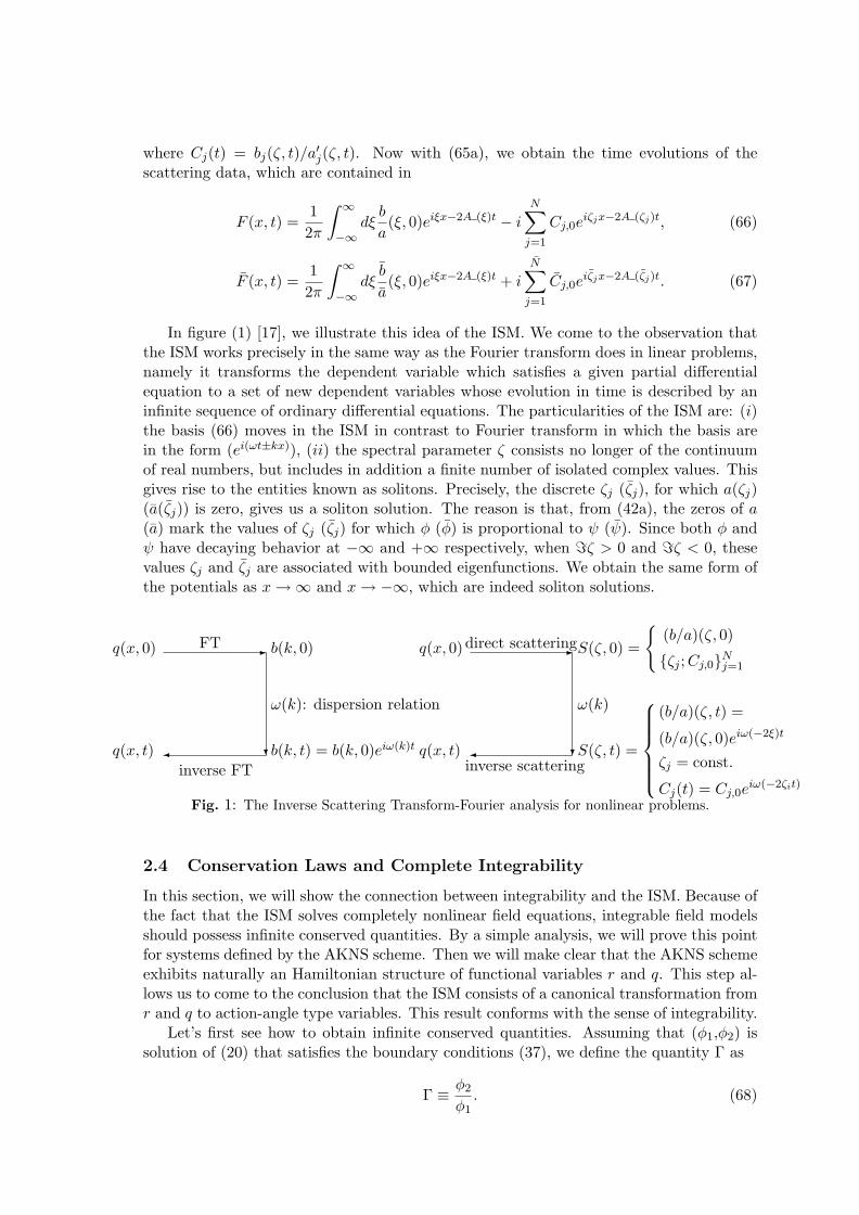
In figure (1) [17], we illustrate this idea of the ISM. We come to the observation thatthe ISM works precisely in the same way as the Fourier transform does in linear problems,namely it transforms the dependent variable which satisfies a given partial differentialequation to a set of new dependent variables whose evolution in time is described by aninfinite sequence of ordinary differential equations. The particularities of the ISM are: (i)the basis (66) moves in the ISM in contrast to Fourier transform in which the basis arein the form (ei(ωt±kx)), (ii) the spectral parameter ζ consists no longer of the continuumof real numbers, but includes in addition a finite number of isolated complex values. Thisgives rise to the entities known as solitons. Precisely, the discrete ζj (ζj), for which a(ζj)(a(ζj)) is zero, gives us a soliton solution. The reason is that, from (42a), the zeros of a(a) mark the values of ζj (ζj) for which φ (φ) is proportional to ψ (ψ). Since both φ andψ have decaying behavior at −∞ and +∞ respectively, when =ζ > 0 and =ζ < 0, thesevalues ζj and ζj are associated with bounded eigenfunctions. We obtain the same form ofthe potentials as x→∞ and x→ −∞, which are indeed soliton solutions.
-
?q(x, t)
q(x, 0) direct scattering
inverse scatteringS(ζ, t) =
(b/a)(ζ, t) =
(b/a)(ζ, 0)eiω(−2ξ)t
ζj = const.
Cj(t) = Cj,0eiω(−2ζit)
S(ζ, 0) =
(b/a)(ζ, 0)
ζj ;Cj,0Nj=1
ω(k)
-
?q(x, t)
q(x, 0)FT
inverse FTb(k, t) = b(k, 0)eiω(k)t
b(k, 0)
ω(k): dispersion relation
Fig. 1: The Inverse Scattering Transform-Fourier analysis for nonlinear problems.
2.4 Conservation Laws and Complete Integrability
In this section, we will show the connection between integrability and the ISM. Because ofthe fact that the ISM solves completely nonlinear field equations, integrable field modelsshould possess infinite conserved quantities. By a simple analysis, we will prove this pointfor systems defined by the AKNS scheme. Then we will make clear that the AKNS schemeexhibits naturally an Hamiltonian structure of functional variables r and q. This step al-lows us to come to the conclusion that the ISM consists of a canonical transformation fromr and q to action-angle type variables. This result conforms with the sense of integrability.
Let’s first see how to obtain infinite conserved quantities. Assuming that (φ1,φ2) issolution of (20) that satisfies the boundary conditions (37), we define the quantity Γ as
Γ ≡ φ2
φ1. (68)
By direct calculations, i.e. deriving (68) with respect to t and x and using (20), (21) and(29), we obtain the local conservation equation
(qΓ)t = (BΓ +A)x, (69a)
where A and B are functions in the evolution operator T , and the Riccati equation
Γx = 2iζΓ + r − qΓ2. (69b)
From Appendix (C), we can see that as |ζ| → ∞, φ1eiζx and φ2e
iζx evolve as
φ1eiζx = 1− 1
2iζ
∫ x
−∞r(y)q(y)dy +©(
1ζ2
), (70a)
φ2eiζx = − 1
2iζr(x) +©(
1ζ2
). (70b)
Hence Γ→ 0, as |ζ| → ∞. We may expand Γ in inverse power of ζ
Γ =∞∑n=1
Γn(x, t)(2iζ)n
. (71)
Substituting this into (69b) yields
Γ1 = −r, Γn+1 = Γnx + q
n−1∑k=1
ΓkΓn−k, for n ≥ 1. (72)
From (69a), it follows that
∂
∂t
∞∑n=1
qΓn(2iζ)n
=
∂
∂x
A+
B
q
∞∑n=1
Γn(2iζ)n
. (73)
The conserved quantities are expressed as
Cn =∫ ∞−∞
qΓndx. (74)
Thus the first conserved quantities are
C1 =∫ ∞−∞−(qr)dx, C2 =
∫ ∞−∞
(−qrx) dx, (75)
C3 =∫ ∞−∞
[−qrxx + (qr)2
]dx, C4 =
∫ ∞−∞
(−qrxxx + 4q2rrx + r2qqx
). (76)
For example, in the case where r = σq∗ with σ = ±1 and
A = −2iζ2 − iσ|q|2, B = 2ζq + iq, (77)
we have the NLS equation. Substituting these into (73) yields
∂t
[ ∞∑n=1
qΓn(2iζ)n
]+ i∂x
[2ζ2 + σ|q|2 + (2iζq − qx)
∞∑n=1
Γn(2iζ)n
]= 0. (78)
The first local conservation laws are
n = 1, ∂t[|q|2] + i∂x[qq∗x − q∗qx] = 0, (79)
n = 2, ∂t[−qq∗x] + i∂x[|qx|2 − qq∗xx + σ|q|4] = 0. (80)
As t plays the role of parameter in the auxiliary problem (20), we assume the systems areat t = 0, and we drop the time dependence for the moment. From Appendix (C), we knowthat for =ζ > 0, both a(ζ) and φ1e
iζx approach to 1 as |ζ| → ∞, moreover, from (37), wecan see
a(ζ) = limx→∞
φ1eiζx. (81)
We may express φ1 asφ1 = exp(−iζx+ φ), (82)
with φ vanishes as |ζ| → ∞. Substituting (82) into (20) gives us
φx = qΓ. (83)
From (74) and (83), we have
φ(x→∞) =∫ ∞−∞
dxqΓ. (84)
Since a are time-independent, taking log of a gives us
log a(ζ) = φ(x = +∞) =∞∑n=1
Cn(2iζ)n
, (85)
where Cn is defined as (74). This result conforms with our definition of Cn. From Appendix(D), we can deduce an explicit expression of log a(ζ)
log a(ζ) =∞∑n=1
ζ−n
N∑m=1
1n
[(ζ∗m)n − (ζm)n]
−(2πi)−1
∫ ∞−∞
ξ(n−1)
[log aa(ξ) +
N∑m=1
logξ − ζ∗mξ − ζm
+N∑l=1
logξ − ζ∗mξ − ζm
]dξ
.
(86)
Note that this expression must coincide with that in (74), so that for n = 1, 2, 3, . . . ,
Cn = − 1π
∫ ∞−∞
(2iξ)n[
log aa(ξ) +N∑m=1
logξ − ζ∗mξ − ζm
+N∑l=1
logξ − ζ∗mξ − ζm
]dξ
+N∑m=1
1n
[(2iζ∗m)n − (2iζm)n] . (87)
If r = ±q∗, these simplify to
Cn = − 1π
∫ ∞−∞
(2iξ)n log |a(ξ)|2dξ +N∑m=1
1n
[(2iζ∗m)n − (2iζm)n] . (88)
These are the ”trace formulae” for (20). They relate the infinite set of conserved constants,Cn, to moments of log a(ζ) and the powers of the discrete eigenvalues.
Now we present the Hamiltonian structure of (20). We can state the general theoremthat: if A is an entire function of ζ in the form
Aζ =12i
∞∑n=1
(−2ζ)n−1an (89)
then the system defined by (20) and (21) is Hamiltonian. q(x, t) and r(x, t) are the conju-gate variables and the appropriate Hamiltonian is
H(q, r) = i∞∑n=0
anCn(q, r)(i)n, (90)
where Cn is defined by (74). The prove of this theorem can be found in [17, 15]. We canalso show that the equations of motion can be written in the form
qt =δH
δr, and rt = −δH
δq. (91)
Define the Poission structure
A,B =∫ ∞−∞
(δA
δq
δB
δr− δA
δr
δB
δq
). (92)
We can immediately see the infinite set of conserved quantities Cn are all in involution by
0 =dCndt
=∫ ∞−∞
δCnδq
∂q
∂t+δCnδr
∂r
∂t
dx
=∫ ∞−∞
δCnδq
δH
δr− δCn
δr
δH
δq
dx (93)
= Cn, H (94)
We can rewrite the Hamiltonian by substituting (87) into (90),
H =(
2π
)∫ ∞−∞
A (ζ)
log a(ζ)a(ζ) +N∑m=1
logξ − ζ∗
ξ − ζm+
N∑l=1
logξ − ζ∗lξ − ζl
dξ+4iN∑m=1
∫ ζm
ζ∗m
A (ζ)dζ.
(95)Define a new pair of variables P (ζ) and Q(ζ) in the following way, for ζ real, i.e. ζ = ξ,
P (ξ) = loga(ξ) ¯a(ξ), Q(ξ) = − 1π
log b(ζ). (96)
There may be discrete eigenvalues for =ζ > 0,
a(ζm) = 0, cm =b
a′|ζm , m = 1, . . . , N, (97a)
and for ζ < 0,
a(ζj) = 0, cj =b
a′|ζj , j = 1, . . . , N. (97b)
Let
Pm = ζm, Qm = −2i log cm, m = 1, . . . , N, (98a)Pl = ζl, Ql = −2i log cl, l = 1, . . . , N . (98b)
Denote by S the variables defined in (96) and (98). We can show that the mapping(r, q) → S is a canonical transformation with the Hamiltonian defined in (95). Now itis apparent that H depends on the generalised momenta (P (ζ), Pm, Pl), but not on thecoordinates (Q(ζ), Qm, Ql). This is the defining property of action-angle variables. It isalso apparent that Hamilton’s equation take the form
∂P
∂t= 0,
∂Q
∂t=δH
δP. (99)
Thus, P is time-independent variable, while Q evolves linearly in time. Explicitly, we have
∂
∂t(log aa(ξ)) = 0,
∂
∂t(log b(ξ)) = −2A (ξ), for ζ ∈ R, (100a)
∂
∂tζm = 0,
∂
∂t(log cm) = −2A (ζ), m = 1, . . . , N, (100b)
∂
∂tζl = 0,
∂
∂t(log cl) = −2A (ζ), l = 1, . . . , N . (100c)
These results lead us to the conclusion that the ISM is indeed a canonical transformation(r, q)→ S, and the variables S lead us to action-angle variables.
3 Exact Solution of Nonlinear Schrodinger Equation
In this section, we will use the ISM to solve the nonlinear Schrodinger equation (NLS)
iut + uxx − 2σ|u|2u = 0, where σ = ±. (101)
3.1 Soliton Solution
In Appendix (E), we will prove that if σ = +1 the coefficient a(ζ) has no zero in the upperhalf complex plane of ζ. Hence, there is no soliton solution. This result conforms withour physical intuition: if σ = +1, the interaction being repulsive in (101), there will beno bounded state, while if σ = −1, the interaction being attractive, we may have solitonsolution.
Provided that σ = −1 and b = 0 which corresponds to the reflectionless condition i.e.there is no reflection in the auxiliary problem, we will take N = 1, i.e. a(ζ) has one zeroin the upper half plane. Consequently (66) becomes
F (x, t) = −iC(t)eiζx, ζ = ξ + iη, and η > 0. (102)
Dropping for the moment the time-dependence, and substituting (102) into (48) yields
K1(x, y) = iC∗e−iζ∗(x+y) −
∫ ∞x
∫ ∞x
K1(x, z)|C|2eiζzeis(ζ−ζ∗)e−iζ∗ydsdz. (103)
Define K1(x) =∫∞x K1(x, z)eiζzdz. Multiplying (102) by eiζy and operating it with
∫∞x dy,
we get
K1(x) = − C∗ei(ζ−2ζ∗)x
ζ − ζ∗[1−
(|C|2e2i(ζ−ζ∗)x/(ζ − ζ∗)2
)] . (104)
From a direct calculation of (103), we can have K1(x, y) in terms of K1 in the form
K1(x, y) =iC∗e−iζ∗(x+y) − |C|2
∫ ∞x
dzK1(x, z)eiζz∫ ∞x
dseis(ζ−ζ∗)e−iζ
∗y
=iC∗e−iζ∗(x+y) − |C|2K1(x)
(−eiζ∗yei(ζ−ζ∗)x
i(ζ − ζ∗)
). (105)
Substituting the expression of K1 into (105) gives us
K1(x, y) = iC∗eiζ(x+y)
[1− |C|2
(ζ − ζ∗)2e2i(ζ−ζ∗)x
]. (106)
Then the potential q(x) is given by
q(x) = −2K1(x, x) = − 2iC∗e−2iξx
e2ηx +(|C|24η2
)e−2ηx
. (107)
Putting the time evolution in C wiht C(t) = C0e−2A (ζ)t. Since A (ζ) = 2iζ2, we have
C = C0e−4iζ2t. Defining C0 = |C0|eiψ0 , x0 = log |C0|/2η, we obtain the usual expression
for q(x, t),q(x, t) = 2ηe−2iξxe4i(ξ2−η2)t−i(ψ0+π
2)sech(2ηx− 8ξηt− x0). (108)
3.2 General Solution of ISM
We will express the solution of the NLS equation in a general form by the ISM. Recallthat from section (2.3), we have the general setting
r = σq∗, σ = ±1, q = −2K(x, x), (109)
K(x, y) = σF ∗(x+ y)− σ∫ ∞x
ds1
∫ ∞x
dz1K(x1, z1)F (z1 + s1)F ∗(s1 + y), (110)
where
F (x) ≡ 12π
∫c
b
a(ζ)eiζxdζ, (111a)
F ∗(x) ≡ 12π
∫c
b∗
a∗(ζ∗)e−iζxdζ. (111b)
We can express F (x) and F (x) in a more general form
F (x) =∫Cλ(k) exp(ikx)dk, (112a)
F ∗(x) =∫Cλ∗(k∗) exp(−ik∗x)dk∗, (112b)
where C presents the complex plane of k, ζ in (111) is replaced by k, λ(k) ∝ ba(k) and
λ∗(k∗) ∝ b∗
a∗ (k∗), and dk and dk∗ present some appropriate measures in C which keep (111)
and (112) equivalent. Iterating K in the integral equation (110), we have
K = σF ∗(x, y)− σ2
∫ ∞x
ds1dz1F∗(x+ z1)F (z1 + s1)F ∗(s1 + y)
+ σ3
∫ ∞x
ds1ds2dz1dz2F∗(x+ z2)F (z2 + s2)F ∗(s2 + z1)F (z1 + s1)F ∗(s1 + y) + . . .
= K0 +K1 +K2 + · · · =∞∑n=0
Kn, (113)
with
Kn = (−1)nσn+1
∫[x,∞]2n
ds1 . . . dsndz1 . . . dzn
∫C2n+1
dp∗1 . . . dp∗n+1dq1 . . . dqn×
exp
−ip∗n+1x+ in∑
α=1
(qα − p∗α+1zα) + in∑β=1
(qβ − p∗β)sβ − ip∗1y
= (−1)nσn+1
∫C2n+1
dp∗1 . . . dp∗n+1dq1 . . . dqn×
n∏j=1
[∫ ∞x
dsjdzj exp(i(qj − p∗j+1)zj + i(qj − pj)sj)]
exp(−ip∗n+1x− ip∗1y)
= (−1)nσn+1
∫C2n+1
dp∗1 . . . dp∗n+1dq1 . . . dqn
n∏j=1
Ij
exp(−ip∗n+1x− ip∗1y). (114)
We can calculate directly Ij with
Ij =∫ ∞x
dsjdzj exp(i(qj − p∗j+1)zj + i(qj − pj)sj)
=
(1
iqj − ip∗j+1
)[exp(iqj − ip∗j+1)zj
]∞x
(1
iqj − ip∗j
)[exp(iqj − ip∗j )sj
]∞x
= −
(1
qj − p∗j+1
× 1qj − p∗j
)exp(i(qj − ip∗j+1)x+ i(qj − p∗j )x). (115)
Hence we have
Kn =(−σ)n+1
∫C2n+1
dp∗1 . . . dp∗n+1dq1 . . . dqn
n∏j=1
dqj
(1
qj − p∗k+1
)(1
qj − p∗k
)×
exp[ix(2qj − p∗j − p∗j+1)
]exp
[−i(p∗n+1x+ p∗1y)
]. (116)
Adding the time dependence for λ(k, t) in accord with (65) in knowing that A (k) = 2ik2,we have
λ(k, t) = λ(k) exp(−i4k2t
), (117a)
λ∗(k∗, t) = λ∗(k∗) exp(i4(k∗)2t
). (117b)
Define the following measures∫dλ(k2j+1) =
∫−dp∗j , with − p∗j → k2j+1, (118a)∫
dµ(k2j) =∫dqj , with qj → k2j , (118b)
where j = 1, 2, . . . , n. With the relation between p∗j and qj , we can see that dµ∗(−k∗) =dλ(K). Doing some appropriete scaling between x and t, and absorbing the extra mul-tiplicative terms in (exp) into the measures dλ(k2j+1) and dµ(k2j), we can finally obtain
the general solution of nonlinear Schrodinger equation written in the form
q(x, t) =∞∑n=0
m=2n+1
σm∫Cm
exp (iΩm(x, t))∏2nj=1(kj + kj+1)
dλ1dµ2dλ3dµ4 . . . dλm, (119)
|q(x, t)|2 = ∂x
∞∑n=1
σn−1
∫Cm
(−1) exp (iΩ2n(x, t))∏2n−1j=1 (kj + kj+1)
dλ1dµ2 . . . dµ2n−1dλ2n, (120)
where Ωn =n∑j=1
[kjx+ (−1)jk2
j t]. (121)
4 Defect Problem
Generally speaking, a defect in 2D (1D space + 1D time) integrable field theories can beviewed as internal boundary conditions in the domain where the field u(x, t) is defined. In[4, 5], Bowcock, Corrigan and Zambon introduced a Langrangian formalism to generatedefects in the classical integrable models in keeping the systems completely integrable. Inthis section, we present another approach [6], introduced by Caudrelier, which uses theISM in the AKNS scheme to generate defects. Integrability is proved systematically byconstructing the generating function of the infinite set of modified integrals of motion. Thecontribution of the defects to all orders will be explicitly identified in terms of a defectmatrix.
Consider a following system: choose a point x0 ∈ R and suppose that the auxiliaryproblem exists for x > x0 with the operators X and T , and for x < x0 with T and X . Xand T are defined in the form
X =(−iζ qr iζ
)≡ −iζσ3 +W, with W =
(0 qr 0
), and T ≡
(A BC −A
), (122)
and X and T are defined in the same way. We assume that these two systems are connectedby
v(x, t, ζ) = L(x, t, ζ)v(x, t, ζ), (123)
at x = x0, where L(x, t, ζ) is called defect matrix which links the solutions of two sides ofx0. From the general definitions (122) and (123), we can obtain
Lx = XL− LX , (124a)
Lt = T L− LT . (124b)
We now introduce the generating function I(ζ) for the integral of motions
I(ζ) = IL(ζ) + IR(ζ) + ID(ζ), (125)
where
, IL(ζ) =∫ ∞−∞
qΓdx, (126a)
IL(ζ) =∫ ∞−∞
qΓdx, (126b)
ID(ζ) =− log(L11 + L12Γ)|x=x0 , (126c)
and Lij are the entries of the defect matrix L. Let’s prove this formula. From the definitionof two first elements of I(ζ), we have
∂t
∫ ∞−∞
qΓdx+ ∂t
∫ ∞−∞
qΓdx = (BΓ + A− (BΓ +A))|x=x0 . (127)
By using (122) to both u and u, from (126a) and (126b) we can have
∂t
∫ ∞−∞
qΓdx+ ∂t
∫ ∞−∞
qΓdx =(L11 + L12Γ)t(L11 + L12Γ)
|x=x0 , (128)
which corresponds the derivative of (126c) with respect to t. Hence
∂tI(ζ) = 0. (129)
Then we suppose that L(x, t, ζ) may be expanded in inverse power of ζ,
L(x, t, ζ) =N∑n=0
Ln(x, ζ)ζ−n. (130)
For n = 1,L(x, t, ζ) = L0(x, ζ) + ζ−1L1(x, ζ). (131)
Substituting this form into (124a) gives
0 =[L0, σ3], (132a)
L0x =i[L1, σ3] + WL0 − L0W, (132b)
L1x =WL1 − L1W. (132c)
If T and T are polynomials in ζ with coefficients Tj and Tj , where j = 0, . . . , N , from(132) and (124b), we have the relations for Tj (Tj),
L1t =T0L1 − L1T0, (133a)
L0t =T1L1 − L1T1 − T0L0 − L0T0, (133b)
0 =T2L1 − L1T2 + T1L0 − L0T1, (133c)... (133d)
0 =TNL0 − L0TN . (133e)
Finally, we can show that (the proof is established in [6]) for n = 1 of (130), L(x, t, ζ) canbe written
L = I + ζ−1
12
a+ ±
[a2 − 4a2a3
] 12
a2
a312
a+ ∓
[a2 − 4a2a3
] 12
, (134)
wherea2 = − i
2(q − q), a3 =
i
2(r − r), (135)
and a± ∈ C are the (x, t-independent) parameters of the defect. For example, if q = u,r = σq∗, σ = ±, u is a complex scalar field. L can be written
L = I + ζ−1
12
a+ ± i
√b2 + σ|u− u|2
− i
2(u− u)
− i2σ(u∗ − u∗) 1
2
a+ ∓ i
√b2 + σ|u− u|2
, (136)
where b = ia1 ∈ R. Hence the defect matrices are determined by two arbitrary variablesa+ and b. Taking into account r = σq∗, it turns out that the real integral of the motionscan be expressed in the following combination
Ireal(ζ) = i(I(ζ)− I∗(ζ∗)), (137)
and the contribution of defect can be written
IDreal(ζ) = −i (log(L11 + L12Γ)− log(L11 + L12Γ)∗) . (138)
Expand (137) in inverse power of ζ, and adding (138), we can obtain the expression ofmodified conserved quantities. For the first three conserved quantities, we have
Cm =∫ x0
−∞|u|2dx+
∫ ∞x0
|u|2dx∓ σΣσ|x=x0 , (139a)
Pm = i
∫ x0
−∞(uu∗x−u∗ux)dx+i
∫ ∞x0
(uu∗x−u∗ux)dx−i [(u∗u− uu∗ ∓ 2σbΣσ)] |x=x0 , (139b)
Hm =∫ x0
−∞
(|ux|2 + σ|u|4
)dx+
∫ x0
−∞
(|ux|2 + σ|u|4
)dx[
∓Σσ
(|u|2 + |u|2
)∓ σ
3Σσ
(3b2 − Σ2
σ
)− ib (uu∗ − uu∗)
]|x=x0 . (139c)
This method stands for the AKNS scheme, the same procedure can so be done for otherintegrable nonlinear equations.
5 Conclusions and Outlook
In this report, I have presented the Inverse Scattering method to solve integrable nonlin-ear evolution equations under the boundary conditions where u(x, t) → 0 as |x| → ∞.The AKNS scheme provides a simple and efficient framework to identify and solve sys-tematically nonlinear equations. On one hand we can consider the ISM as a Fourier-typetransform of nonlinear equations, on the other hand in showing that the AKNS schemeexhibits naturally a Hamiltonian structure, the ISM can be regarded as a canonical trans-formation which make the systems being written in terms of action-angle variables. In thecontext of classical integrable models, an ISM approach to generate defects, which keepsystems completely integrable, has also been shown.
There are numerous alternative questions which are related to the ISM presented here.First the ISM in the AKNS scheme is not the unique way to solve nonlinear equations.Zakharov and Shabat [24] introduced a direct version of the ISM, called dressing method byusing an operator formalism. Furthermore, the procedure of obtain the Gel’fand-Levitan-Marchenko equation is closely related to Riemann-Hilbert problems in complex analysis.There exist also Hirota’s bilinear method [10], Backlund transformation...etc. We expectthat all these methods are related one to another. In addition, the AKNS scheme andthe ISM can be generalised in a matrix form [21, 20], where the field u(x, t) will representa vector. From another point of view, the study of integrability reveals a rich algebraicstructure. The classical r-matrix can be also involved in the ISM. The correspondingHamiltonian structure can be transported to the quantum case.
Based on this project, some developments are possible for future work. We can generatethe defect matrices to matrix generalisation of integrable models. Moreover, we can extendthe defect problem to other contexts other than the AKNS scheme. Finally, a generalisationof what we present here will be to put defects in a random way in our integrable systems.
Acknowledgments
I would like to acknowledge Vincent Caudrelier, my supervisor, who introduced me intothe field of Mathematical Physics and accompanied me in the course of this project. Ithank warmly Andrea Cavaglia for numerous discussions and encouragements. I extendalso my gratitude to all people who helped me both in my study and in my life during mystay in London, especially Andreas Fring, Olalla Castro-Alvaredo, Qinna Wang.
Appendices
A KdV Hierarchy
I will show how Lax obtained the evolution operatorM for the spectral operator L whichis defined as a 1D Schrodinger operator
L = − d2
dx2+ u(x, t). (140)
Lax marked that L(t) is unitarily equivalent to L(0), i.e. there exists an linear operatorU on a Hilbert space H which satisfies
U(t)L(t)U(t) = L(0), and U(t)U(t) = I, (141)
where U is the adjoint of U , i.e. (ψ,Uφ) = (Uψ, φ). According to (141), operating on afunction φ ∈ H with UL(t) gives
UL(t)φ = L(0)Uφ. (142)
Doing the inner product to the two sides of (142) with φ, we have
(φ, UL(t)φ) = (φ, Uλ(t)φ) = λ(t)(Uφ, φ), (143a)
(φ,L(0)Uφ) = (U L(0)φ, φ) = λ(0)(Uφ, φ). (143b)
Thus, λ(t) = λ(0), the L(t) has the same eigenvalue as L(0). Now define M on H as
Ut =MU, and M = −M. (144)
Deriving (142) with respect to t yields
0 =UtLU + ULtU + UtLUt=UMLU + ULtU + UtLMU
=U(ML+ Lt + LM)U
=U (Lt − [L,M])U. (145)
Hence, L and M are indeed a Lax pair satisfying
Lt − [L,M] = 0. (146)
From the definition (144), we know that M is a linear operator which is to be anti-symmetric so that −(Mφ, ψ) = (φ,Mψ) for all φ, ψ ∈ H. A natural choice is therefore to
construct M from a suitable linear combination of odd derivatives in x. (Consider innerproduct (φ, ψ) =
∫∞−∞ φψdx, then
(Mφ, ψ) =∫ ∞−∞
∂nφ
∂xnψdx =
∫ ∞−∞
φ∂nψ
∂xndx = −(φ,Mψ), (147)
if n is odd and φ, φx, . . . , ψ, ψx, · · · → 0 as x→ ±∞.) The simplest choice is obviously
M = c∂
∂x, (148)
and this gives usut − cux = 0. (149)
For a third-order differential operator, we have the general form
M = −α ∂3
∂x3+ V
∂
∂x+
∂
∂xV +A, (150)
where α is a constant, V = V (x, t) and A = A(x, t). This operator identifies with (17b)with a suitable choice that α = 4, V = 3
4αu and A = A(t). Thus, the KdV equation hasappeared as the second example within the framework of the Lax pair. It is the first non-trivial case. The procedure adopted above can now be extended to higher-order nonlinearevolution equations. With M defined as
M = −α ∂2n+1
∂x2n+1+
n∑m=1
(Vm
∂2m−1
∂2m−1x+
∂2m−1
∂2m−1xVm
)+A. (151)
For n = 2, it can be shown that the evolution equation is
ut + 30u2ux − 20uxuxx − 10uuxxx + uxxxx = 0, (152)
which presents a fifth-order KdV equation. Clearly, there is an infinity of evolution equa-tions, and we call the class of equations obtained in this way the KdV hierarchy.
B Proof of Analyticity of φiζx
I will prove the statement of the analyticity of φiζx in section (2.3). For ζ = ξ + iη, andη > 0, operating
∫ x−∞ dy to φ2y(y, ζ)eiζy gives,∫ x
−∞dyφ2y(y, ζ)eiζy =
[φ2(y, ζ)eiζy
]x−∞− iζ
∫ x
−∞dyφ2(y, ζ)eiζy,
=φ2(x, ζ)eiζx − iζ∫ x
−∞dyφ2(y, ζ)eiζy. (153)
Multiplying eiζx to the second line of (20), changing the variable x to y and operating onit with
∫ x−∞ dy, we have
φ2(x, ζ)eiζx = 2iζ∫ x
−∞dyφ2(y, ζ)eiζy +
∫ x
−∞dyr(y)φ1(y, ζ)eiζy. (154)
Deriving (154) with respect to x, and putting
f(x, ζ) = φ2(x, ζ)eiζx, g(x, ζ) = r(x)φ1(x, ζ)eiζx, (155)
yieldd
dxf(x, ζ) = 2iζf(x, ζ) + g(x, ζ). (156)
By solving this differential equation of 1st order, we have
φ2(x, ζ)eiζx =∫ x
−∞dyr(y)e2iζ(x−y)φ1(y, ζ)eiζy. (157)
In the same way, multiplying eiζx to the first line of (20), changing x to y and operatingon it with
∫ x−∞ dy, we obtain
φ1(x, ζ)eiζx =1 +∫ x
−∞dyq(y)φ2(y)eiζy,
=1 +∫ x
−∞dy
∫ y
−∞dzq(y)r(z)e2iζ(y−z)φ(z, ζ)eiζz. (158)
Setting
R0(x) ≡∫ x
−∞|r(y)|dy, Q0(x) ≡
∫ x
−∞|q(y)|dy, (159)
we can show that
|φ1(x, ζ)eiζx| ≤1 +∫ x
−∞dy1
∫ y
−∞dz1q(y1)r(z1)φ1z1, ζ
≤1 +∫ x
−∞dy1
∫ x
−∞dz1|q(y1)||r(z1)|
(1 +
∫ z1
−∞dy2
∫ z1
−∞dz2|q(y2)||r(z2)|
(1 +
∫ z2
−∞
∫ z2
−∞. . . .
(160)
With∫ x
−∞
∫ x
−∞
∫ z1
−∞
∫ z1
−∞. . .
∫ zn−1
−∞
∫ zn−1
−∞
n∏j=1
(dyjdzj) =(
1n!
)∫ x
−∞. . .
∫ x
−∞︸ ︷︷ ︸2n×
R x−∞
n∏j=1
(dyjdzj) ,
(161)
we have
|φ1(x, ζ)eiζx| ≤1 +Q0(x)R0(x) +12!Q0(x)2R0(x)2 +
13!Q0(x)3R0(x)3 + . . .
=I0(2√Q0(x)R0(x))). (162)
where I0 is the modified Bessel function which is absolutely convergent. So φ1eiζx is
bounded. The analyticity of φ1eiζx can be easily established by repeating the same proce-
dure by differentiating (158) with respect to ζ. In the same way, we can see that ψ(x, ζ)eiζx
is also analytic in the upper half plane (η > 0), while φe−iζx and ψ(x, ζ)eiζx are analyticin the lower half plane (η < 0). From (42a), a(ζ) and a(ζ) are respectively analytic in theupper and lower half plane.
Furthermore, by direct calculations of the expressions of (157) and (158), we can obtainthe asymptotic behaviors of φ1e
iζx and φ2eiζx as |ζ| → ∞,
φ1eiζx = 1− 1
2iζ
∫ x
−∞r(y)q(y)dy +©(
1ζ2
), (163a)
φ2eiζx = − 1
2iζr(x) +©(
1ζ2
). (163b)
Similar expressions can be obtains for φe−iζx, ψe−iζx and ψeiζx. With these asymptoticexpansions and (42), as |ζ| → ∞ we have the asymptotic expressions of a and a,
a(ζ) = 1− 12iζ
∫ ∞−∞
r(y)q(y)dy +©(1ζ2
), (164a)
a(ζ) = 1 +1
2iζ
∫ ∞−∞
r(y)q(y)dy +©(1ζ2
). (164b)
C Symmetry Relations between q and r
The symmetry relations between q and r in (20) yield some interesting results for thetransition coeffients a (b) and a (b).
Assuming r = ±q∗, (20) becomes
ux =(−iζ q±q∗ iζ
)u, or iζu =
(−∂x q∓q∗ ∂x
)u. (165)
With our usual definition of φ (ψ) and φ (ψ) satisfying the boundary conditions (37), wecan obtain the following relation(
φ∗2x(x, ζ∗)φ∗1x(x, ζ∗)
)=(−iζ∗ ±qq∗ iζ∗
)(φ∗2(x, ζ∗)φ∗1(x, ζ∗)
). (166)
This identifies with (165) with the symmetric property that ζ → ζ∗, u1 → ∓φ∗2(x, ζ∗) andu2 → φ∗1(x, ζ∗). Note that ( ∓φ∗2, φ∗1(x, ζ∗)) satisfy the boundary condition for φ. Similarrelations can be obtain for ψ and ψ, and we can come to the following results,
φ(x, ζ) =(∓φ∗2(x, ζ∗)−φ∗1(x, ζ∗)
), ψ(x, ζ) =
(ψ∗2(x, ζ∗)±ψ∗1(x, ζ∗)
), (167)
which imply that
a(ζ) = a∗(ζ∗), b(ζ) = ∓b∗(ζ∗), (168a)N = N, ζk = ζ∗k , Ck = ∓C∗k . (168b)
In the same way, in the case where r = ±q, we have
φ(x, ζ) =(∓φ2(x,−ζ)φ1(x,−ζ)
), ψ(x, ζ) =
(ψ2(x,−ζ)±ψ1(x,−ζ)
), (169)
and
a(ζ) = a(−ζ), b(ζ) = ∓b(−ζ), (170a)N = N, ζk = −ζk, Ck = ∓Ck. (170b)
D Proof of Expression of log a
We have stated in the section (2.4) that the conserved quantities are known once log a isknown for =ζ > 0. Now we will show how to obtain the expression of log a [15, 17]. Recallthat a(ζ) is analytic for =ζ > 0 with a finite number of zeros, and a→ 1 as |ζ| → ∞. We
also assume that: (i) the zeros of a are simple, (ii) no zero occurs on the real axis, (iii)for real ξ, ξn log a(ξ)→ a as |ξ| → ∞ for all n ≥ 0. Define α(ζ) as
α(ζ) = a(ζ)N∏m=1
ζ − ζ∗mζ − ζm
, (171)
α(ζ) shares these same analytic properties as a(ζ), but with no zero for =ζ > 0. Similarly,a(ζ) is analytic in the lower half plane, and we can define α(ζ) as
α(ζ) = a(ζ)N∏l=1
ζ − ζ∗lζ − ζl
. (172)
α(ζ) is analytic with no zero in the half plane where=ζ ≤ 0 and it tends to 1 as ζ → ∞.By Cauchy’s integral theorem, for =ζ ≥ 0, we have
logα(ζ) =1
2πi
∫ ∞−∞
logα(ξ)ξ − ζ
dξ, (173a)
0 =1
2πi
∫ ∞−∞
log α(ξ)ξ − ζ
dξ. (173b)
By adding these, we find that, for =ζ ≥ 0,
log a(ζ) =N∑m=1
logζ − ζmζ − ζ∗m
+
12πi
∫ ∞−∞
log (α(ξ)α(ξ))ξ − ζ
dξ. (174)
If we further assume that r = ±q∗, this simplifies to
log a(ζ) =N∑m=1
logζ − ζmζ − ζ∗m
+
12πi
∫ ∞−∞
log |α(ξ)|2(ξ)ξ − ζ
dξ. (175)
Keeping =ζ > 0, we can expand the right side of (174), as |ζ| → ∞ in inverse power of ζ
log a(ζ) =∞∑n=1
ζ−n
N∑m=1
1n
[(ζ∗m)n+1(ζm)n+1
]−(
12πi
)∫ ∞−∞
ξn
[log aa(ξ) +
N∑m=1
logξ − ζ∗mξ − ζm
+N∑l=1
logξ − ζ∗mξ − ζm
]dξ
.
(176)
This expression corresponds to (86) in section (2.4).
E Proof of No Zeros of a for (σ > 0) in (3.1)
As we have seen, the NLS equation (101) can be recasted into the relation r = ±q∗ in theAKNS scheme. According to (21), we can express the auxiliary problem as an eigenvalueproblem Lv = ζv, where
L =(i∂x −iqσiq∗ −i∂x
), and σ = ±1. (177)
If σ = +1, we can show that L is a self-adjoint operator, thus it can only have realeigenvalues. Suppose that there exists a ζ0 such that a(ζ0) = 0 with =ζ0 > 0. It followsfrom (42a) that the vectors φ and ψ are linearly dependent. Since =ζ0 > 0, φ and ψhave exponential decay behaviors as x → −∞ and x → ∞ respectively. Thus (20) has asolution v decaying exponentially as |x| → ∞. However (20) is equivalent to the eigenvalueproblem (21), in which the self adjoint operator L would have real eigenvalue ζ ′0. Thiscontradiction leads us to the conclusion that a(ζ) has no complex zeros, i.e. there are nozeros in the upper half plane. No soliton solutions occur if σ = +1. If σ = −1, L is notself-adjoint, and a(ζ) may have zeros.
Bibliography
[1] M. J. Ablowitz, D. J. Kaup, A. C. Newell, and H. Segur. Method for solving thesine-gordon equation. Phys. Rev. Lett., 30(25):1262–1264, Jun 1973.
[2] V.I. Arnold. Mathematical Methods of Classical Mechanics. Springer, 1989.
[3] P.N. Bibikov and V.O. Tarasov. Boundary-value problem for nonlinear schrAudingerequation. Theoretical and Mathematical Physics, 79:570–579, June 1989.
[4] P. Bowcock, E. Corrigan, and C. Zambon. Affine Toda field theories with defects.Journal of High Energy Physics, 1:56–+, January 2004.
[5] P. Bowcock, E. Corrigan, and C. Zambon. Classically Integrable Field Theories withDefects. International Journal of Modern Physics A, 19:82–91, 2004.
[6] V. Caudrelier. On a Systematic Approach to Defects in Classical Integrable FieldTheories. International Journal of Geometric Methods in Modern Physics, 5:1085–+,2008.
[7] Clifford S. Gardner, John M. Greene, Martin D. Kruskal, and Robert M. Miura.Method for solving the korteweg−devries equation. Phys. Rev. Lett., 19(19):1095–1097, Nov 1967.
[8] C.S. Gardner. Kortewegde vries equation and generalizations. iv. the korteweg−devries equation as a hamiltonian system. Journal of Mathematical Physics, 12, Dec.1970.
[9] I.M. Gel’fand and B.M. Levitan. On the determination of a differential equation fromits spectral function. Izv. Akad. Nauk SSSR Ser. Mat., 15:309–360, 1951.
[10] R. Hirota. The direct method in soliton theory. Cambridge University Press, 2004.
[11] J. Ieda, M. Uchiyama, and M. Wadati. Inverse scattering method for square matrixnonlinear Schrodinger equation under nonvanishing boundary conditions. Journal ofMathematical Physics, 48(1):013507–+, January 2007.
[12] D.J. Kaup and P.J. Hansen. An initial-boundary value problem for the nonlinearschrAudinger equation. Physica D: Nonlinear Phenomena, 18:77–84, Jan 1986.
[13] D.J. Korteweg and G. de Vries. On the change of form of long waves advancingin a rectangular channel and on a new type of long stationary waves. Phil. Mag,39:422–443, 1895.
[14] P.D. Lax. Integrals of Nonlinear Equations of Evolution and Solitary Waves. Commun.Pure Appl. Math, 21:467–490, 1968.
[15] L.A. Takhtajan L.D. Faddeev. Hamiltonian Methods in the Theory of Solitons.Springer, 2007.
[16] A.C. Newell H. Segur M.J. Ablowitz, D.J. Kaup. The Inverse Scattering Transform-Fourier Analysis for Nonlinear Problems. Studies in Applied Mathematics, 1974.
[17] H. Segur M.J. Ablowitz. Solitons and the Inverse Scattering Transform. Studies inApplied Mathematics, 1981.
[18] P.A. Clarkson M.J. Ablowitz. Solitons, Nonlinear Evolution Equations and InverseScattering. Studies in Applied Mathematics, 1991.
[19] M. Talon O. Babelon, D. Bernard. Introduction to Classical Integrable Systems. Cam-bridge University Press, 2003.
[20] T. Tsuchida and M. Wadati. The Coupled Modified Korteweg−de Vries Equations.J. Phys. Soc. Jpn, 67:1175–1187, December 1998.
[21] M. Wadati. The Modified Kortewegde Vries Equation. J. Phys. Soc. Japan, 34:5,1972.
[22] V.E. Zakharov and L.D. Faddeev. Korteweg−de vries equation: A completely inte-grable hamiltonian system. Journal Functional Analysis and Its Applications, 5:422–443, Oct. 1971.
[23] V.E. Zakharov and A.B. Shabat. Exact theory of two-dimensional self-focusing andone-dimensional self-modulation of waves in nonlinear media. Soviet Physics, 34:62–69, Jan 1972.
[24] V.E. Zakharov and A.B. Shabat. A scheme for integrating the nonlinear equations ofmathematical physics by the method of the inverse scattering problem. i. FunctionalAnalysis and Its Applications, 8:226–235, 1974.