Zeroth-Order Implicit Reinforcement Learning for

Zeroth-Order Implicit Reinforcement Learning for SequentialDecision Making in Distributed Control Systems

Vanshaj Khattar Qasim Wani∗ Harshal Kaushik Zhiyao Zhang∗ Ming JinVirginia Tech Virginia Tech Virginia Tech Xiangtan University Virginia Tech

Abstract

Despite being reliable and well-established,convex optimization models, once built, donot adapt to the changing real-world con-ditions or fast evolving data streams. Suchrigidness may lead to higher costs andeven unsafe scenarios, rendering traditionalmodel-based approaches inadequate for mod-ern distributed control systems (DCSs).Recently, learning-based techniques haveachieved remarkable success in operating sys-tems with unknown dynamics; nevertheless,it is difficult to include safety and assur-ance during the online process. We pro-pose a novel zeroth-order implicit reinforce-ment learning framework for adaptive deci-sion making in DCSs. We solve the sequentialdecision making problem with a policy classbased on convex optimization. The reinforce-ment learning (RL) agent aims to adapt theparameters within the optimization model it-eratively to the dynamically changing condi-tions. This approach enables us to includegeneral constraints within the RL framework.We also improve the convergence of the pro-posed zeroth-order method by introducing aguidance mechanism. Our theoretical anal-ysis of the non-asymptotic global conver-gence rate reveals the benefits of the guid-ance factor. The effectiveness of our pro-posed method is validated on two real-worldapplications, including a recent RL competi-tion, showing a significant improvement overexisting algorithms.

*Works completed during the summer internship in Dr.Ming Jin’s group as undergraduate researchers.

1 Introduction

Sequential decision making problems appear in nu-merous domains, such as energy, supply chain man-agement, finance, health, and robotics to name afew. The major challenge in these applications is tomake decisions under uncertainty (that may arise inthe forms of uncertain demands of electricity, goods,changing prices, and unstable weather), which may beattributed to various factors such as dynamic environ-ments and human interventions. A large class of prob-lems involve distributed control systems, where theobjective is to control multiple systems to achieve adesired objective while satisfying domain-specific con-straints (Zhou et al., 2020; Wilson et al., 2020).

Reinforcement learning is promising for DCSs for twokey reasons. First, it allows the agent to act withoutthe need of a predefined model—a feature of particularinterests for large-scale, complex systems, where it isnot cost-effective to develop such a model and informa-tion sharing is fundamentally limited. Also, by contin-uously adapting the agent to the environment, RL cansystematically account for dynamic uncertainty andenvironmental drift. Notably, RL agents are rarely de-ployed in a standalone manner but as part of a largerpipeline with infrastructures and humans in the loop.Thus, it is imperative for RL agents to make real-timedecisions that respect constraints on their physical andsocial ramifications. Recently, (Dulac-Arnold et al.,2021) identified a set of challenges for real-world RL(all pertinent to DCSs). We are poised to addressseven out of the nine challenges in the present study (asevidenced in the success of our method in a recent RLcompetition, detailed in Section 4), including: 1) theability to learn on live systems from limited samples;2) learning and acting in high-dimensional state andaction spaces; 3) reasoning about system constraintsthat should never or rarely be violated; 4) interactingwith systems that are partially observable, which canalternatively be viewed as systems that are stochas-tic; 5) learning from multiple objectives; 6) the abilityto provide actions quickly; and 7) providing systemoperators with explainable policies.

Zeroth-order Implicit RL

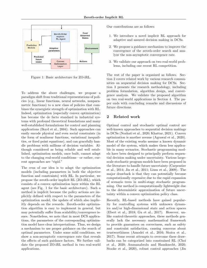
Figure 1: Basic architecture for ZO-iRL.

To address the above challenges, we propose aparadigm shift from traditional representations of poli-cies (e.g., linear functions, neural networks, nonpara-metric functions) to a new class of policies that com-bines the synergistic strength of optimization with RL.Indeed, optimization (especially convex optimization)has become the de facto standard in industrial sys-tems with profound theoretical foundations and manywell-established formulations for control and planningapplications (Boyd et al., 2004). Such approaches caneasily encode physical and even social constraints (inthe form of nonlinear functions, variational inequali-ties, or fixed point equations), and can gracefully han-dle problems with millions of decision variables. Al-though considered as being reliable and well estab-lished, optimization models, once built, cannot adaptto the changing real-world conditions—or rather, cur-rent approaches are “rigid.”

The crux of our idea is to adapt the optimizationmodels (including parameters in both the objectivefunction and constraints) with RL. In particular, wepropose the zeroth-order implicit RL (ZO-iRL), whichconsists of a convex optimization layer within the RLagent (see Fig. 1 for the basic architecture). Such amethod is implicit because the policy actions are im-plicitly defined with respect to the parameters of theoptimization model, the update of which also implic-itly depends on the rewards. Zeroth-order optimiza-tion algorithm is easy to implement in general, butmay potentially suffer from scalability/convergence is-sues. Nonetheless, we note that in most DCS applica-tions, the parameters of the corresponding optimiza-tion model have clear interpretations. Thus, we designa mechanism to use proper guidance on the search ofoptimal parameters. Under some mild conditions, weshow a non-asymptotic convergence rate that revealsthe effects of such guidance factors. We further vali-date the proposed ZO-iRL method in two real-worldapplications.

Our contributions are as follows:

1. We introduce a novel implicit RL approach foradaptive and assured decision making in DCSs.

2. We propose a guidance mechanism to improve theconvergence of the zeroth-order search and ana-lyze the non-asymptotic convergence rate.

3. We validate our approach on two real-world prob-lems, including one recent RL competition.

The rest of the paper is organized as follows. Sec-tion 2 covers related work by various research commu-nities on sequential decision making for DCSs. Sec-tion 3 presents the research methodology, includingproblem formulation, algorithm design, and conver-gence analysis. We validate the proposed algorithmon two real-world applications in Section 4. The pa-per ends with concluding remarks and discussions offuture directions.

2 Related work

Optimal control and stochastic optimal control arewell-known approaches to sequential decision makingsin DCSs (Nozhati et al., 2020; Khattar, 2021). Convexoptimization is another avenue (Agrawal et al., 2020).Most of the existing works assume a known dynamicmodel of the system, which makes them less applica-ble in many scenarios. Stochastic programming mod-els have been designed to principally perform sequen-tial decision making under uncertainty. Various large-scale stochastic program models have been proposed inthe literature to handle future uncertainty (Carpentieret al., 2014; Jin et al., 2011; Lium et al., 2009). Themajor drawback is that they can potentially becomecomputationally expensive due to the rapid expansionof scenario trees in multi-stage stochastic program-ming. Our method is computationally lightweight dueto the deterministic approximation of future uncer-tainty within a convex optimization policy class.

Recently, RL-based methods have gained popular-ity for controlling systems with unknown dynam-ics and/or high-dimensional state and action spaces(Ebert et al., 2018; Gu et al., 2017). However, un-like control-theoretic approaches, these methods gen-erally lack the necessary mathematical frameworkto provide guarantees on correctness, such as safetyand constraint satisfaction, causing concerns abouttrustworthiness (Amodei et al., 2016; Stoica et al.,2017). Some recent attempts to overcome these draw-backs can be categorized into constrained RL (Choiet al., 2020; Ammanabrolu and Hausknecht, 2020;Stooke et al., 2020), robust control approaches (Jin

and Lavaei, 2020; Yin et al., 2021; Gu et al., 2021),Lyapunov-based methods (Berkenkamp et al., 2017;Chow et al., 2018; Perkins and Barto, 2002), Hamil-ton–Jacobi reachability methods (Gillula and Tom-lin, 2012; Fisac et al., 2018), control-barrier func-tions (Ames et al., 2016; Cheng et al., 2019; Deanet al., 2020; Qin et al., 2021), and robust MPC (Hew-ing et al., 2020). Lately, game-theoretic approacheshave emerged to coordinate multiple systems in DCSs(Zhang et al., 2021). Our method is a step forwardin the area of Constrained RL. The prime advantageof our method is that it is adaptive to any applica-tions due to the simplicity and ubiquity of convex op-timization control policies. Donti et al. (2021) alsointroduces an optimization layer based on Lyapunovguarantees for safety. However, their method requiresmodel information and is first-order. Our method ismodel-free and zeroth-order (under guidance).

The present work is closely related to (Agrawal et al.,2020; Ghadimi et al., 2020), which share the lineof thinking that uses convex optimization as a pol-icy class to handle uncertainty. In (Agrawal et al.,2020), convex optimization control policies are learnedby tuning the parameters within the convex opti-mization layer. We extend their method to systemswith unknown dynamics by incorporating a lookaheadmodel (predictions) in our formulation. The paramet-ric cost function approximation (PCFA) framework in(Ghadimi et al., 2020) is limited to linear or affinePCFAs. We extend their method to parametric con-vex cost functions approximations inspired by manyattractive properties of convex optimization models(Agrawal et al., 2020).

3 Methodology

3.1 Problem formulation

Consider a sequential decision making problem in aDCS with N subsystems, each controlled by an agent.Furthermore, we allow couplings among different sub-systems within the DCS, so that the evolution of onesubsystem may affect the states of the others. Thegoal is to learn an optimal policy for each agent thatminimizes the overall cost over a period of evaluation.

Formally, we aim to find a set of optimal policiesΠ = {π1, π2, ..., πN} for each agent in the DCS thatminimizes an objective function defined over a finitetime horizon T :

minΠ={π1,...,πN}

E

[T∑

t=0

N∑i=1

Ct,i

(xit, πi(x

it), {xl

t}l∈L(i)

)],

(1)where xi

t ∈ Rni is the state of the i-th subsystemat time t; πi : Rni → Rmi is the policy of agent i,

so πi(xit) is the action taken at time t. Let xi

t+1 =fMi

(xit, πi(x

it),W

it+1) be the state transition function

for the i-th subsystem, which is unknown to us. Weuse the random variable W to capture the random-ness from all possible sources, the realization of whichfor subsystem i at time t + 1 is represented by W i

t+1.Note that the expectation is taken over the initialstates and the random variable W (which may af-fect the state transitions). Denote the cost functionas Ct,i : Rni+mi → R, so Ct,i

(xit, πi(x

it), {xl

t}l∈L(i)

)represents the cost incurred at time t for subsystemi under policy πi, where {xl

t}l∈L(i) represents the col-lection of states of the set of subsystems L(i) coupledwith subsystem i.

Problem (1) is not possible to address in practice be-cause of the unknown underlying dynamics and ran-domness involved. To solve for the optimal policies in(1), we employ a lookahead model formulation (Powelland Meisel, 2015) to account for the impact of presentdecision on the future outcomes. Thereby, the optimalpolicy at time t can be computed as

π⋆i (x

it) = argmin

πi

(Ct,i

(xit, πi(x

it), {xl

t}l∈L(i)

)+

E

[T∑

t′=t+1

Ct′,i

(xit′ , πi(x

it′)∣∣∣xi

t, πi(xit)

])(2)

The formulation in (2) can also be seen as a Bellmanequation. The main challenge in solving (2) is that theobserved costs usually contain noise and are random innature (true for many real-world applications). Costsof agent i are also dependent on the the actions of theothers.

3.2 Zeroth-order implicit RL framework

To solve (2), we construct a surrogate convex cost func-tion Ct,i, which is parametrized by some parametersζi = {ζi1, · · · ζiT }. This allows us to write (2) as:

π⋆i (x

it|ζi) = argmin

π⋆i

(Ct,i

(xit, πi(x

it)|ζi

)+

T∑t′=t+1

Ct,i

(xit′ , πi(x

it′)|ζi)

) (3)

where xit′ are the predicted future states, ζi ∈ Rdi

is a di-dimensional parameter vector associated withthe i-th subsystem, and it considers a decentralizedsetting where the agent can only access its own state(but not others). Construction of such a surrogateconvex cost function should be such that desired be-havior is encouraged. This is closely related to the


reward design problem in RL (Prakash et al., 2020).Formulation (3) is a convex optimization problem thatcan be solved, provided that the estimates of the fu-ture states are reliable. The optimized policy obtainedfrom (3) can be directly applied to the environment.The overall goal of (1) can now be restated as: find thebest possible parameters for (3), such that optimal pol-icy being deployed in environment achieves minimumcost. This motivates the ZO-iRL method, where theRL-agent finds the best possible parameters for thesurrogate convex cost function Ct,i. The policy that isbeing deployed in the environment will be computedafter solving the implicit convex optimization prob-lem. The ZO-iRL framework can be formulated (andunderstood) as a bilevel optimization problem:

ζi = argminζi

E

[T∑

t=0

Ct,i

(xit, π

⋆i (x

ti), {xl

t}l∈L(i)|ζi)]

,

(4)where the policy π⋆

i (xit′ |ζi) is obtained after solving

an implicit convex optimization problem for the i-thsubsystem with a fixed instantiation of parameters ζi:

π⋆i (x

it|ζi) = argmin

π⋆i

(Ct,i

(xit, πi(x

it)|ζi

)+

T∑t′=t+1

Ct,i

(xit′ , πi(x

it′)|ζi)

)subject to gj(x

it, πi(x

it)) ≤ 0 ; j ∈ I

hj(πi(xit)) = 0 ; j ∈ E ,

(5)

where gj : Rmi+ni → R for all j =∈ I are convex inπi(x

it) and hj : Rmi → R for all j ∈ E are affine in

πi(xit).

This bilevel optimization framework consists of anouter optimization layer (4) and an implicit convexoptimization layer (5). The RL agent (outer layer) isrepresented using (4) with the aim to learn the param-eters ζi that minimize the observed costs Ct,i in theenvironment. The observed costs Ct,i are dependenton the optimal policy computed by the implicit convexoptimization layer.

3.3 Guided random search

This section presents the method for the RL agent tolearn the optimal parameters within the convex opti-mization layer, namely, to solve the outer layer opti-mization problem. The parameters of an optimizationmodel often carry clear physical meanings—in prac-tice, they are typically set by experts based on ex-perience or system specifications. Thus, we propose aguidance mechanism that enables the search algorithmto leverage such domain knowledge for faster and ro-bust convergence. This zeroth-order method, given in

Algorithm 1 ZO-iRL Algorithm

Input: Nc, σ, ρ, P1 = N (0, σ2), k = 1Output: ζ⋆

1: for k=1,2, · · · do

2: Sample Nc candidates from the distribution

Pk: ζ(k)1 , ζ

(k)2 , · · · , ζ(k)Nc

3: for j = 1, · · ·Nc do4: For each agent, adopt the policy (5)

parametrized by ζ(k)j to control its corre-

sponding subsystem over the horizon T

5: Observe cost C(ζ(k)j ) provided by sampling

from the objective function of (4)6: end for7: Sort theNc candidates on the basis of costs ob-

tained. Let ζ⋆1 and ζ⋆2 be the best parameters.

8: Calculate A(k)g = mean(ζ⋆1 , ζ

⋆2 )

9: Compute the guidance for each of the candi-date by:

G(ζ(k)j ) = ζ

(k)j + ρ(A(k)

g − ζ(k)j ) (6)

10: Compute the new probability distributionPk+1 for the next:

Pk+1(dζ) =

Nc∑j=1

r(k)j T

(ζ(k)j , dζ

)(7)

where:

r(k)j =

exp[−Ct(ζ(k)j )]∑Nc

j=1 exp[−Ct(ζ(k)j )]

(8)

T (ζ(k)j , dζ) = N (G(ζ

(k)j ), σ2)µ(dζ) (9)

and µ is a fixed probability measure on (Z,B)11: Increment k → k + 1

Algorithm 1, is partly inspired by the “method of gen-erations” (see (Zhigljavsky, 2012)).

In a nutshell, at each iteration, the algorithm ran-domly samples a set of candidates for exploration. Thesampling distribution is determined by the noisy costsobserved for the previous candidates. In particular,for agent i at time t, we observe a noisy cost sample j:

Ct(ζ(k)j ) = ftrue(ζ

(k)j ) + wk(ζ

(k)j ) (10)

where ftrue is the underlying true cost function that wecannot observe (corresponding to the objective in (4))

and wk(ζ(k)j ) is the random noise at iteration k. The

visualisation of the Algorithm 1 is given in the Fig. 2.

Figure 2: Visualization of the guidance mechanism inAlgorithm 1.

3.4 Convergence rate analysis

We now prove that the sequence generated by ZO-iRLis guaranteed to converge to an optimal solution andshow the non-asymptotic convergence rate. We adoptthe following notations: Z is a compact metric space;B is the σ−algebra of Borel-subsets of Z; and ζ ∈ Zn

is the collection of parameters to be learned, where nis its ambient dimension.

For the convergence analysis, we explicitly state thefollowing assumptions:

1. The disturbance wk(ζ) is a random variable withzero mean distribution F (ζ, dw) that is concen-trated within a finite interval [−d, d].

2. The random variables wk(ζ) are independent forall candidate k and parameter ζ ∈ Z

3. The transition probability function is given by

T (ζ(k)j , dζ) = κ(ζ

(k)j , ζ

(k+1)j )µ(dζ), and is always

bounded, with µ a probability measure on (Z,B):

supζ(k)j ,ζ

(k+1)j ∈Z

κ(ζ(k)j , ζ

(k+1)j ) ≤ Λ < ∞

4. There exists a permutation order ν such that themagnitude of difference between the generated

value ζ(k+1)ν(j) from the guided value of the previ-

ous sample ζkj is bounded by twice of the guidancefactor ρ using the following equation:

|ζk+1ν(j) −G(ζkj )| ≤ 2ρ

5. There exists a global optimal solution ζ⋆, andthere exists an ϵ > 0, such that the underlying

true objective function ftrue is continuous in theset B(ζ⋆, ϵ).

We note that Assumption 5 is a much more relaxedcondition than requiring differentiability (Agrawalet al., 2020). The following theorem shows the con-vergence rate of generated distributions Pk(dζ) to astationary distribution SNc .

Theorem 3.1. Under the assumptions listed above:

1. For any number of candidates Nc, the random

elements ak = (ζ(k)1 , · · · , ζ(k)Nc

) form a homoge-neous Markov chain with a stationary distributionSNc

(dζ1, · · · , dζNc).

2. Pk(dζ) converges to SNcwith a geometric rate that

depends on Nc, guidance factor ρ, and variance σ2 asfollows:

supB∈BN

∣∣Pk(B)− SNc(B)

∣∣ ≤ (1− c2)k−1 (11)

where c2 =

[Ncc1e

−2ρ2/σ2

c1+(Nc−1) exp[mf+d]σ√2π

]Nc

with mf de-

note the maximum value of ftrue within a compactset of parameters, and c1 = inf E[Ct(ζ)], and given0 < c2 < 1

Detailed proof of Theorem 3.1 can be found in thesupplementary material.

Deciding the value of the guidance factor: Forthe result of Theorem 3.1 to be valid, we need to have0 < c2 < 1. The introduction of the guidance factorρ can ensure that c2 always stays between 0 and 1.Moreover, a good choice of ρ can make c2 closer to 1,which, by our analysis, may lead to a faster conver-gence of Pk(dζ) to the stationary distribution SNc

.

To keep 0 < c2 < 1, we need limit the following ratio::

Ncc1e−2ρ2/σ2

c1 + (Nc − 1)exp[mf + d]σ√2π

∈ (0, 1) (12)

We propose that to have a fast convergence rate, areasonable value for k1 should be between 0.6 and 1.This implies:

0.6 <e−2ρ2/σ2

σ√2π

k1 < 1, (13)

where

k1 =Ncc1

c1 + (N − 1)exp[mf + d]. (14)


Based on (13), a reasonabale range for the guidancefactor can be:

σ√2

√ln(k1)− ln(σ

√2π) < ρ <

σ√2

√ln(k1)− ln(0.6σ

√2π)

(15)

While the exact determination of the relevant param-eters may be difficult in some situations, the aboveinequality provides some quantitative relation of aproper value for the guidance factor with respect tothe noise variance and other properties of the prob-lem.

4 Experiments

We consider two applications to validate the proposedZO-iRL algorithm. Source code can be found in thesupplementary material, and will be made available tothe public upon publication.

4.1 Profit maximization for a network ofsupply chains

Problem Definition: As presented in (Agrawal et al.,2020), the goal is to find a set of policies for a net-work of supply chains that maximizes profit. We notethat the problem setting is simpler than the presentstudy, because 1) the dynamics and future states areassumed to be known, and 2) only a one-time decisionis required, obviating the need of a lookahead model.

A network of supply chains contains n interconnectedwarehouses, m links over which goods can flow, k linksthat connect suppliers to warehouses, c links that con-nect warehouses to customers, with the rest of them− k − c links represent the internode connections.

Let ht ∈ Rn+ denote the amount of goods held at each

node at time t, pt ∈ Rk+ denotes the price at which the

warehouses can buy from suppliers at time t, r ∈ Rc+

characterize the fixed process for sale to consumers,dt ∈ Rc

+ be the uncertain consumer demand at time t.The decision variables include: 1) bt ∈ Rk

+ (the quan-tity to buy from suppliers); 2) st ∈ Rc

+ (the quantity

to be sold to to the customers); and 3) zt ∈ Rm−k−c+

(the quantity to be shipped across internode links).The holding costs for goods is given by αTht + βTh2

t ,where α, β ∈ Rn

+.

The true cost to minimize can be accessed directlywithout additional noise, and is given by:

1

T

T−1∑t=0

pTt bt − rT st + τT zt + αTht + βT (hTt .ht) (16)

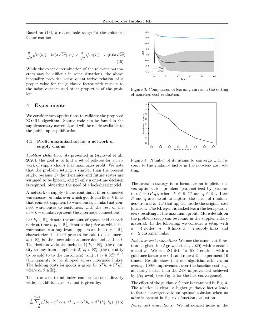
Figure 3: Comparison of learning curves in the settingof noiseless cost evaluation.

0.0 0.1 0.2 0.3 0.4 0.5 0.6 0.7Guidance Factor

10

11

12

13

14

15

16

17

18

itera

tions

to c

onve

rge

Figure 4: Number of iterations to converge with re-spect to the guidance factor in the noiseless cost set-ting.

The overall strategy is to formulate an implicit con-vex optimization problem, parametrized by parame-ters ζ = (P, q), where P ∈ Rn×n and q ∈ Rn. HereP and q are meant to capture the effect of random-ness from α and β that appear inside the original costfunction. The RL agent is tasked learn the best param-eters resulting in the maximum profit. More details onthe problem setup can be found in the supplementarymaterial. In the following, we consider a setup withn = 4 nodes, m = 8 links, k = 2 supply links, andc = 2 customer links.

Noiseless cost evaluation: We use the same cost func-tion as given in (Agrawal et al., 2020) with constantα and β. We run ZO-iRL for 100 iterations with aguidance factor ρ = 0.1, and repeat the experiment 10times. Results show that our algorithm achieves onaverage 109% improvement over the baseline cost, sig-nificantly better than the 24% improvement achievedby (Agrawal) (see Fig. 3 for the fast convergence).

The effect of the guidance factor is examined in Fig. 4.The relation is clear: a higher guidance factor leadsto faster convergence to an optimal solution when nonoise is present in the cost function evaluation.

Noisy cost evaluations: We introduced noise in the

Figure 5: Comparison of learning curves in the settingof noisy cost evaluation.

0.0 0.1 0.2 0.3 0.4 0.5 0.6 0.7Guidance Factor

20

40

60

80

100

itera

tions

to c

onve

rge

Figure 6: Number of iterations to convergence withrespect to the guidance factor in the noisy cost setting.

cost function evaluation by introducing randomness inthe parameters α and β to make the setup closer to thereal world scenarios. We ran our method again for 100iterations with a guidance a factor ρ = 0.5. This setupwas run 10 times and our method not only improvedthe baseline cost from 0.83 to an average of −2.455but also exhibits more stable learning as compared toCOCP’s experiments. (Agrawal et al., 2020) approachwas only able to improve the baseline cost only from0.83 to −0.483, and also exhibits unstable behaviorsin the presence of noise.

The effect of guidance is shown in Fig. 6. In this case,there is no simple relation between the guidance factorand convergence rate, consistent with our theoreticalanalysis. Indeed, as shown in (15), the best range ofrho depends on a host of variables. It appears thata reliable choice of the guidance factor should be be-tween 0.5 and 0.7.

4.2 CityLearn Challenge

Problem definition: The CityLearn Challenge is an an-nual competition aimed to inspire RL solutions to ad-dress grand challenges for the control of power grids(Vazquez-Canteli et al., 2020a). This competition is

motivated by the pressing needs for climate changemitigation and adaptation by enhancing energy flexi-bility and resilience in the face of climate-induced de-mand surge (as already observed in places like Califor-nia, where rolling blackouts are increasingly frequentduring the Summer) and natural adversity (such asthe disastrous winter storm in Texas and extreme heatwaves in India and Iran this year). It provides a setof benchmarks for evaluating AI-based methods in co-ordinating distributed energy resources for intelligentenergy management.

The competition has an online setup with only oneepisode of the entire 4 years, when agents will exploitthe best policies to optimize the coordination strat-egy. Notably, CityLearn encompasses all the chal-lenges discussed in the Introduction section, including1) the ability to learn on live systems from limitedsamples—there is no training period; 2) learning andacting in high-dimensional state and action spaces—the RL agents need to coordinate 9 individual build-ings; 3) dealing with system constraints that shouldnever or rarely be violated—there are strict balanc-ing equations for electricity, heating, and cooling en-ergy; 4) interacting with systems that are partiallyobservable—it is a distributed control setup; 5) learn-ing from multiple objectives—the evaluation metricsinclude ramping cost, peak demands, 1-load factor,carbon emissions; 6) the ability to provide actionsquickly—there is a strict time limit for completing the4 year evaluation on Google’s Colab; and 7) providingsystem operators with explainable policies—a neces-sity to facilitate real-world adoption and deployment.For more information on the simulation setup, we referto (Vazquez-Canteli et al., 2020a)

To model the implicit convex optimization layer, wefirst construct a surrogate convex cost function to pro-mote desirable behaviors such as load flattening andsmoothing. As a proxy for the competition evaluationmetrics, the surrogate cost function at time t is givenby:

Ct,i = |Egridt − Egrid

t−1 |+ pelet Egridt +

T∑t′=t+1

(|Egrid

t′ − Egridt′−1|+ pelet′ E

gridt′

) (17)

where Egridt is the electricity demand for a building at

time t. The RL agents aim is to learn the parame-ter pele ∈ R24 (separately for each of the 9 buildings)that represents the virtual electricity cost. The con-straints of the optimization model include energy bal-ance equations and technological constraints, and canbe found in the supplementary material. We model


MethodClimateZone

Ramping1-LoadFactor

Avg. DailyPeak

PeakDemand

Net Elec.Consumption

Avg.Score

ZO-iRL

1 0.833 1.010 0.986 0.953 1.002 0.9642 0.784 1.025 0.962 0.961 1.001 0.9563 0.822 1.048 0.989 0.955 1.001 0.9694 0.743 0.990 0.974 1.006 1.002 0.9535 0.711 0.999 0.9691 0.939 1.004 0.924

Average Score 0.953

SAC

1 2.470 1.202 1.354 1.209 1.049 1.3902 2.413 1.183 1.349 1.152 1.056 1.3693 2.609 1.1185 1.382 1.313 1.056 1.4354 2.512 1.168 1.376 1.207 1.057 1.3975 1.614 1.115 1.133 1.159 1.015 1.177

Average Score 1.353

RandomAgent

1 1.071 1.130 1.168 1.077 0.993 1.0732 1.045 1.138 1.151 1.079 0.987 1.0663 1.032 1.131 1.158 1.180 0.991 1.0814 0.965 1.101 1.114 1.134 0.984 1.0485 1.015 1.138 1.116 1.089 0.987 1.057

Average Score 1.065

MARLISA

1 1.02 1.019 1.015 1.0 1.0 1.0092 1.008 1.02 1.012 1.0 0.998 1.0063 1.002 1.017 1.01 1.0 0.999 1.0054 1.002 1.029 1.014 1.0 0.998 1.0075 1.39 1.105 1.103 1.205 1.001 1.136

Average Score 1.032

Table 1: Scores for ZO-iRL and comparison methods,including SAC (Kathirgamanathan et al., 2020) andMARLISA (Vazquez-Canteli et al., 2020b). The ran-dom agent basically uniformly selects an action withinthe range at each timestep.

this problem using the lookahead model, where a set ofpredictors are designed to predict future states basedon the past 2 weeks data. The competition evaluatesperformance of RL agents by computing the ratio ofcosts with respect to a deterministic rule-based con-troller (RBC). Therefore, a lower ratio indicates a bet-ter performance.

Table 1 shows the scores of our ZO-iRL agent com-pared to existing baseline. Note that MARLISA istailor-designed for the competition Vazquez-Canteliet al. (2020b). All agents are validated on data from5 different climate zones. It can be observed that ZO-iRL has achieved the lowest cost ratios (i.e. the bestscores) as compared to baseline methods. In particu-lar, baseline RL methods struggle to learn a reasonablepolicy within the limited 4-year test period, while ZO-iRL is able to quickly find a good policy within thefirst few months (see Fig. 7). Furthermore, the learn-ing progress can be intuitively explained by inspectingthe evolution of parameter pele as shown in Fig. 8. Inthis particular case, the building tends to overchargeits storage in the early morning, which results in unex-pected electricity peaks that is undesirable; by increas-ing the virtual prices during that period, the agent isable to find a better strategy that smoothes the peaks,thus resulting in better performance. More details canbe found in the supplementary material.

Figure 7: Learning curve of ZO-iRL, where RBC takesa baseline cost of constant 1.

Figure 8: Evolution of the implicit parameters pele overthe test period, where the values are color-coded.

5 Conclusion and future directions

The present work introduces a novel implicit RLframework for model-free decision making in DCSs.By leveraging the synergistic strength of convex op-timization and RL, the proposed method is able tosimultaneously address a range of challenges for real-world RL. Our work opens up exciting research direc-tions for future works, including the extension of theimplicit RL framework to other derivative-free meth-ods such as Bayesian optimization or first-order meth-ods such as actor-critic RL.

Acknowledgements

The authors would like to thank the organizers of theCityLearn Challenge (Dr. Jose R. Vazquez-Canteli,Dr. Zoltan Nagy, Dr. Gregor Henze, and Sourav Dey)for motivating the proposed approach.

References

Agrawal, A., Barratt, S., Boyd, S., and Stellato, B.(2020). Learning convex optimization control poli-cies. In Learning for Dynamics and Control, pages361–373. PMLR.

Ames, A. D., Xu, X., Grizzle, J. W., and Tabuada,P. (2016). Control barrier function based quadraticprograms for safety critical systems. IEEE Transac-tions on Automatic Control, 62(8):3861–3876.

Ammanabrolu, P. and Hausknecht, M. (2020).Graph constrained reinforcement learning for nat-ural language action spaces. arXiv preprintarXiv:2001.08837.

Amodei, D., Olah, C., Steinhardt, J., Christiano, P.,Schulman, J., and Mane, D. (2016). Concrete prob-lems in ai safety. arXiv preprint arXiv:1606.06565.

Berkenkamp, F., Turchetta, M., Schoellig, A. P., andKrause, A. (2017). Safe model-based reinforcementlearning with stability guarantees. arXiv preprintarXiv:1705.08551.

Boyd, S., Boyd, S. P., and Vandenberghe, L. (2004).Convex optimization. Cambridge university press.

Carpentier, P.-L., Gendreau, M., and Bastin, F.(2014). Managing hydroelectric reservoirs over anextended horizon using benders decomposition witha memory loss assumption. IEEE Transactions onPower Systems, 30(2):563–572.

Cheng, R., Orosz, G., Murray, R. M., and Burdick,J. W. (2019). End-to-end safe reinforcement learn-ing through barrier functions for safety-critical con-tinuous control tasks. In Proceedings of the AAAIConference on Artificial Intelligence, volume 33,pages 3387–3395.

Choi, J., Castaneda, F., Tomlin, C. J., and Sreenath,K. (2020). Reinforcement learning for safety-criticalcontrol under model uncertainty, using control lya-punov functions and control barrier functions. arXivpreprint arXiv:2004.07584.

Chow, Y., Nachum, O., Duenez-Guzman, E., andGhavamzadeh, M. (2018). A lyapunov-based ap-proach to safe reinforcement learning. arXivpreprint arXiv:1805.07708.

Dean, S., Taylor, A. J., Cosner, R. K., Recht, B., andAmes, A. D. (2020). Guaranteeing safety of learnedperception modules via measurement-robust controlbarrier functions. arXiv preprint arXiv:2010.16001.

Donti, P. L., Roderick, M., Fazlyab, M., and Kolter,J. Z. (2021). Enforcing robust control guaranteeswithin neural network policies. In InternationalConference on Learning Representations.

Dulac-Arnold, G., Levine, N., Mankowitz, D. J.,Li, J., Paduraru, C., Gowal, S., and Hester, T.(2021). Challenges of real-world reinforcementlearning: definitions, benchmarks and analysis. Ma-chine Learning, pages 1–50.

Ebert, F., Finn, C., Dasari, S., Xie, A., Lee, A., andLevine, S. (2018). Visual foresight: Model-baseddeep reinforcement learning for vision-based roboticcontrol. arXiv preprint arXiv:1812.00568.

Fisac, J. F., Akametalu, A. K., Zeilinger, M. N., Kay-nama, S., Gillula, J., and Tomlin, C. J. (2018). Ageneral safety framework for learning-based controlin uncertain robotic systems. IEEE Transactions onAutomatic Control, 64(7):2737–2752.

Ghadimi, S., Perkins, R. T., and Powell, W. B. (2020).Reinforcement learning via parametric cost functionapproximation for multistage stochastic program-ming. arXiv preprint arXiv:2001.00831.

Gillula, J. H. and Tomlin, C. J. (2012). Guaran-teed safe online learning via reachability: trackinga ground target using a quadrotor. In 2012 IEEEInternational Conference on Robotics and Automa-tion, pages 2723–2730. IEEE.

Gu, F., Yin, H., Ghaoui, L. E., Arcak, M., Seiler,P., and Jin, M. (2021). Recurrent neural net-work controllers synthesis with stability guaran-tees for partially observed systems. arXiv preprintarXiv:2109.03861.

Gu, S., Holly, E., Lillicrap, T., and Levine, S. (2017).Deep reinforcement learning for robotic manipula-tion with asynchronous off-policy updates. In 2017IEEE international conference on robotics and au-tomation (ICRA), pages 3389–3396. IEEE.

Hewing, L., Wabersich, K. P., Menner, M., andZeilinger, M. N. (2020). Learning-based model pre-dictive control: Toward safe learning in control. An-nual Review of Control, Robotics, and AutonomousSystems, 3:269–296.

Jin, M. and Lavaei, J. (2020). Stability-certified rein-forcement learning: A control-theoretic perspective.IEEE Access, 8:229086–229100.

Jin, S., Ryan, S. M., Watson, J.-P., and Woodruff,D. L. (2011). Modeling and solving a large-scalegeneration expansion planning problem under un-certainty. Energy Systems, 2(3):209–242.

Kathirgamanathan, A., Twardowski, K., Mangina, E.,and Finn, D. P. (2020). A centralised soft actorcritic deep reinforcement learning approach to dis-trict demand side management through citylearn.In Proceedings of the 1st International Workshop onReinforcement Learning for Energy Management inBuildings & Cities, pages 11–14.


Khattar, V. (2021). Threat assessment and proactivedecision-making for crash avoidance in autonomousvehicles.

Lium, A.-G., Crainic, T. G., and Wallace, S. W.(2009). A study of demand stochasticity in servicenetwork design. Transportation Science, 43(2):144–157.

Nozhati, S., Ellingwood, B. R., and Chong, E. K.(2020). Stochastic optimal control methodologies inrisk-informed community resilience planning. Struc-tural Safety, 84:101920.

Perkins, T. J. and Barto, A. G. (2002). Lyapunovdesign for safe reinforcement learning. Journal ofMachine Learning Research, 3(Dec):803–832.

Powell, W. B. and Meisel, S. (2015). Tutorial onstochastic optimization in energy—part i: Modelingand policies. IEEE Transactions on Power Systems,31(2):1459–1467.

Prakash, B., Waytowich, N., Ganesan, A., Oates, T.,and Mohsenin, T. (2020). Guiding safe reinforce-ment learning policies using structured languageconstraints. UMBC Student Collection.

Qin, Z., Zhang, K., Chen, Y., Chen, J., and Fan, C.(2021). Learning safe multi-agent control with de-centralized neural barrier certificates. arXiv preprintarXiv:2101.05436.

Stoica, I., Song, D., Popa, R. A., Patterson, D., Ma-honey, M. W., Katz, R., Joseph, A. D., Jordan, M.,Hellerstein, J. M., Gonzalez, J. E., et al. (2017). Aberkeley view of systems challenges for ai. arXivpreprint arXiv:1712.05855.

Stooke, A., Achiam, J., and Abbeel, P. (2020). Re-sponsive safety in reinforcement learning by pid la-grangian methods. In International Conference onMachine Learning, pages 9133–9143. PMLR.

Vazquez-Canteli, J. R., Dey, S., Henze, G., andNagy, Z. (2020a). Citylearn: Standardizing researchin multi-agent reinforcement learning for demandresponse and urban energy management. arXivpreprint arXiv:2012.10504.

Vazquez-Canteli, J. R., Henze, G., and Nagy, Z.(2020b). Marlisa: Multi-agent reinforcement learn-ing with iterative sequential action selection forload shaping of grid-interactive connected buildings.In Proceedings of the 7th ACM International Con-ference on Systems for Energy-Efficient Buildings,Cities, and Transportation, pages 170–179.

Wilson, S., Glotfelter, P., Wang, L., Mayya, S., No-tomista, G., Mote, M., and Egerstedt, M. (2020).The robotarium: Globally impactful opportunities,challenges, and lessons learned in remote-access, dis-tributed control of multirobot systems. IEEE Con-trol Systems Magazine, 40(1):26–44.

Yin, H., Seiler, P., Jin, M., and Arcak, M. (2021). Imi-tation learning with stability and safety guarantees.IEEE Control Systems Letters.

Zhang, K., Yang, Z., and Basar, T. (2021). Multi-agent reinforcement learning: A selective overviewof theories and algorithms. Handbook of Reinforce-ment Learning and Control, pages 321–384.

Zhigljavsky, A. A. (2012). Theory of global randomsearch, volume 65. Springer Science & Business Me-dia.

Zhou, Q., Shahidehpour, M., Paaso, A., Bahramirad,S., Alabdulwahab, A., and Abusorrah, A. (2020).Distributed control and communication strategies innetworked microgrids. IEEE Communications Sur-veys & Tutorials, 22(4):2586–2633.

Supplementary Material

1 Convergence analysis

We prove a more general version of Theorem 3.1 in the main text that allows the random noises added to eachdimension of the variables to have different standard deviations and inter-parameter correlations. To this end, we

consider a transition function T (ζ(k)j , dζ) = N (G(ζ

(k)j ), σ2)µ(dζ) with a non-singular covariance matrix Σ ∈l×l

(equation (9) in Algorithm 1). The theorem is stated as follows.

Theorem 3.1b. Under the assumptions listed in the main text (Section 3.4):

1. For any number of candidates Nc, the random elements ak = (ζ(k)1 , · · · , ζ(k)Nc

) form a homogeneous Markov

chain with a stationary distribution SNc(dζ1, · · · , dζNc

) with ζi ∈ Rl.

2. Pk(dζ) converges to SNcwith a geometric rate that depends on Nc, guidance factor ρ, and covariance matrix

Σ ∈ Rl×l as follows:

supB∈BN


∣∣ ≤ (1− c2)k−1 (1)

where c2 =

[Ncc1e

−2ρ2/∥Σ∥2

c1+(Nc−1) exp[mf+d]√

(2π)l det(Σ)

]Nc

with mf denote the maximum value of ftrue within a compact

set of parameters, and c1 = inf E[Ct(ζ)], and given 0 < c2 < 1.

Proof. We will first prove that sampling Nc candidate parameters using the ZO-iRL algorithm (see Algorithm 1in the text) can be considered as sampling from a homogeneous Markov chain in the space Zn. Denote thesamples from Zn at iteration k by

ak := (ζ(k)1 , · · · , ζ(k)Nc

). (2)

The initial distribution of the Markov chain is given by

R1(da) = P1(dζ1) · · ·P1(dζNc). (3)

The transition probability of the Markov chain for the sampling process is given by

Q(ak−1, dak) =

∫ d

−d

· · ·∫ d

−d

F (ζ(k−1)1 , dw1) · · ·F (ζk−1

Nc, dwN )

Nc∏j=1

Nc∑i=1

exp[ftrue(ζ(k−1)i ) + wi]∑Nc

l=1 exp[ftrue(ζ(k−1)l ) + wl]

T (ζ(k−1)i , dζj),

(4)

where F (ζ, dw) is the zero-mean distribution for random variable wk(ζ) that is concentrated within a finite

interval [−d, d]. Since the transition probability T (ζ(k−1)i , dζj) is Markovian (by design), the derived transition

probability Q(ak−1, ak) is Markovian. In particular, we can choose the Gaussian distribution:

T (ζ(k−1)i , dζj) =

exp

[−12

((ζ(k) −G(ζ

(k−1)i ))TΣ−1(ζ(k) −G(ζ

(k−1)i )

)]√(2π)l det(Σ)

(5)


Now we will show that the distributions Rk(da) recursively defined by

Rk+1(dak+1) =

∫Zn

Rk(dak)

Nc∏i=1

T (ζ(k)i , dζ) (6)

will converge to a stationary distribution as k → ∞.

In our setting, we can only observe noisy cost samples (instead of the true cost values). It follows from (Loeve,1963, Sec. 29.4) that the random variable for any m defined as

αm :=

∑mi=1 Ct(ζi)

m(7)

will converge for m → ∞ to a random variable α that is independent of αm and Ct(ζi), such that

E[α] = E[Ct(ζi)]. (8)

Now, we proceed to lower bound the transition probability:

Q(ak−1, dak) ≥Nc∏j=1

Nc∑i=1

c1c1 + (Nc − 1)(exp[max(ftrue) + d])

T (ζ(k−1)i , dζj)

≥Nc∏j=1

Nc∑i=1

Ncc1c1 + (Nc − 1)(exp[mf + d])

exp

[−12

((ζ(k) −G(ζ

(k−1)i ))TΣ−1(ζ(k) −G(ζ

(k−1)i )

)]√(2π)l det(Σ)

≥Nc∏j=1

Ncc1c1 + (Nc − 1)(exp[mf + d])

e−2ρ2/∥Σ∥2√(2π)l det(Σ)

= c2µ(dak)

where ∥Σ∥ is the spectral norm of Σ, c1 = inf E[Ct(ζi)], µ(dak) = µ(dζ(k)1 ) · · ·µ(dζ(k)Nc

) is the correspondinglydefined probability measure on (Zn, BNc

), mf denotes the maximum value of ftrue within a compact set ofparameters and

c2 =

[Ncc1e

−2ρ2/∥Σ∥2

c1 + (Nc − 1)exp[mf + d]√(2π)l det(Σ)

]Nc

. (9)

By the results in (Kendall, 1966, Section V.3), we have the following result for the transition probability of thesampled Markov chain:

∆0 = supak−1,ak∈Zn

supB∈BNc

[Q(ak−1, B)−Q(ak, B)] ≤ 1− c2. (10)

Using the exponential convergence criterion (Loeve, 1963), we can conclude that the distributions Rk(dak) willconverge to a stationary distribution SNc

(dak) as k → ∞, where SNcis defined as the unique positive solution

of the following equation:

SNc(dak−1) =

∫Zn

SNc(dak)Q(ak−1, dak) (11)

Moreover, by (Loeve, 1963) we have the following inequalities :

supB∈BNc


∣∣ ≤ ∆k−10 ≤ (1− c2)

k−1. (12)

Thus, the proof is completed. Note that if we specify the covariance matrix to be a diagonal matrix with identicaldiagonal entries, then the result is reduced to Theorem 3.1 in the text.

■

Remarks on theoretical contributions: The proposed algorithm bears resemblance with some existing zeroth-ordermethods, such as cross entropy method (CEM) and evolutionary algorithms (EA); however, most convergenceresults for these algorithms only show asymptotic convergence to an optimal solution with high probability. Inparticular, to the best of the authors’ knowledge, the non-asymptotic convergence rate has not been derivedfor CEM. By contrast, in the present work, we prove that the algorithm yields a convergent sequence with theproperty that the probability distributions Pk will converge to a stationary distribution SNc

at a geometric rate.Some of the recent works have explored the average rate of convergence for EA (Chen and He, 2021). However,their theoretical analysis is based on a martingale-type argument, which only applies to the case where there isno noise in the cost function evaluations. Applicable to a more general setting, our result is able to deal with thenoise in cost function evaluation. Moreover, our convergence result is able to account for the guidance factor.

2 Additional details for experiments

2.1 Profit maximization for a network of supply chains

Denote ht ∈ Rn+ as the amount of goods held at each node at time t, pt ∈ Rk

+ as the price at which the warehousescan buy from suppliers at time t, r ∈ Rc

+ as the fixed process for sales to consumers, dt ∈ Rc+ as the uncertain

consumer demand at time t. The decision variables include: 1) bt ∈ Rk+ (the quantity to buy from suppliers);

2) st ∈ Rc+ (the quantity to be sold to the customers); and 3) zt ∈ Rm−k−c

+ (the quantity to be shipped acrossinternode links). The holding costs for goods is given by αTht + βT ∥ht∥2, where α, β ∈ Rn

+.

The system dynamics are assumed to be known and given by

ht+1 = ht + (Ain −Aout)at, (13)

where Ain ∈ Rn×m and Aout ∈ Rn×m are known matrices, and at is a concatenation of vector-valued decisionvariables including bt, st, and zt.

The following constraints are imposed as part of the supply chain management:

0 ≤ ht ≤ hmax (14a)

0 ≤ bt ≤ bmax (14b)

0 ≤ st ≤ smax (14c)

0 ≤ zt ≤ zmax (14d)

Aoutut ≤ ht (14e)

st ≤ dt (14f)

The uncertainty in future demand and supplier prices are modeled using the log-normal distribution:

logwt := (log pt+1, log dt+1) ∼ N (µ,Σ). (15)

The true cost to minimize is given by

1

T

T−1∑t=0

pTt bt − rT st + τT zt + αTht + βT ∥ht∥2. (16)


The implicit convex optimization layer is parametrized by ζ = (P, q) for some P ∈ Rn×n and q ∈ Rn:

minat=(bt,st,zt)

pTt bt − rT st + τT zt − ||Pht||22 − qTht

s.t. ht+1 = ht + (Ain −Aout)at

0 ≤ ht ≤ hmax

0 ≤ bt ≤ bmax

0 ≤ st ≤ smax

0 ≤ zt ≤ zmax

(17)

Experimental setup: Following (Agrawal et al., 2020), the initial values ht for the network are sampled from auniform distribution between 0 and hmax, where hmax is set to be 3. The maximum for each decision variable isset to be 2. The mean and covariance for the customer demands and the supplier prices are given by

µ = (0, 0.1, 0, 0.4), Σ = 0.04I (18)

In the noiseless cost evaluation setup, we treat the storage cost parameters α and β as known constants withvalues of 0.01. In the noisy cost evaluation setup, we consider the storage cost parameters α and β as randomvariables, with values sampled from a standard normal distribution N (0, 1).

2.2 CityLearn challenge

We refer the reader to (Vazquez-Canteli et al., 2020a) and the corresponding online documentation1 for thedetailed setup of the competition. We will only focus on our strategy in this document. To build a lookaheadmodel for the implicit convex optimization layer, we learn a set of predictors for solar generation and electric-ity/thermal demands. Prediction is done on a rolling-horizon basis for the next 24 hours using the past 2 weeksdata. Denote the hour index by r ∈ {1, 2, · · · , T}, where T = 24. Suppose that we are at the beginning of hourr. Then we need to plan for the action for the upcoming hour r (note that we need to plan for future hours inthe process).

The decision variables for the implicit convex optimization layer at hour r include:

1. Net electricity grid import: Egridt for T ≥ t ≥ r

2. Electricity grid sell: Esellt for T ≥ t ≥ r

3. Heat pump electricity usage: EhpCt for T ≥ t ≥ r

4. Electric heater electricity usage: EehHt for T ≥ t ≥ r

5. Electric battery state of charge: SOCbatt for T ≥ t ≥ r

6. Electrical storage action: abatt for T ≥ t ≥ r

7. Heat storage state of charge: SOCHt for T ≥ t ≥ r

8. Heat storage action: aHstot for T ≥ t ≥ r

9. Cooling storage state of charge: SOCCt for T ≥ t ≥ r

10. Cooling storage action: aCstot for T ≥ t ≥ r

The learnable parameter for the implicit convex optimization layer corresponds to the virtual electricity pricepelet for 1 ≤ t ≤ T . Technology parameters are as follows (we also specify their initializations):

Heat pump technology parameters:

1link: https://sites.google.com/view/citylearnchallenge (Accessed: Oct 21, 2021)

1. Technical efficiency ηhptech = 0.22

2. Target cooling temperature thpC = 8

3. Hourly COP of heat pump COPCt = ηhptech

thpc +273.15

tempt−thpC, where tempt is the outside temperature for hour t for

1 ≤ t ≤ T

4. Heat pump capacity Ehpcmax, estimated from data following a simple statistical procedure

Electric heater parameters:

1. Efficiency ηehH = 0.9

2. Capacity EehHmax, estimated based on a simple statistical procedure

Electric battery:

1. Rate of decay Cfbat = 0.00001

2. Capacity Cpbat, estimated based on a simple statistical procedure

3. Efficiency ηbatt = 1

Heat storage:

1. Rate of decay CfHsto = 0.0008

2. Capacity CpHsto, estimated based on a simple statistical procedure

3. Efficiency ηHstot = 1

Cooling storage:

1. Rate of decay CfCsto = 0.006

2. Capacity CpCsto, estimated based on a simple statistical procedure

3. Efficiency ηCstot = 1

The surrogate objective function is given by:

Ct({Egridt′ }t′≥t) = |Egrid

t − Egridt−1 |+ pelet Egrid

t +

T∑t′=t+1

(|Egrid

t′ − Egridt′−1|+ pelet′ E

gridt′

)(19)

The constraints include both energy balance constraints and technology constraints.Energy balance constraints:

• Electricity balance for each hour t ≥ r:EPV

t + Egridt = ENS

t + EhpCt + EehH

t + abatt Cbatp + Esell

t

• Heat balance for each hour t ≥ r:EehH

t = aHstot CHsto

p +Hbdt

• Cooling balance for each hour t ≥ r:EhpC

t COPCt = aCsto

t CCstop + Cbd

t


Heat pump constraints:

• Maximum cooling for each hour t ≥ r:EhpC

t ≤ EhpCmax

• Minimum cooling for each hour t ≥ r:EhpC

t ≥ 0

Electric heater constraints:

• Maximum limit for each hour t ≥ r:EehH

t ≤ EehHmax

• Minimum limit for each hour t ≥ r:EehH

t ≥ 0

Electric battery constraints:

• Initial SOC:SOCbat

r = (1− Cbatf SOCbat

r−1) + abatr ηbat

• SOC updates for each hour t ≥ r:SOCbat

t = (1− Cbatf )SOCbat

t−1 + abatt ηbat

• SOC terminal condition (note that we set cendbat = 0.1):SOCbat

T = cbatend

• Action limits for each hour t ≥ r:abatlb ≤ abatt ≤ abatub

• Bounds of battery SOC or each hour t ≥ r:1 ≥ SOCbat

t ≥ 0

Heat Storage constraints:

• Initial SOC:SOCH

r = (1− CHstof SOCH

r−1) + aHstor ηHsto

• SOC updates for each hour t ≥ r:SOCH

t = (1− CHstof )SOCH

t−1 + aHstot ηHsto

• Action limits or each hour t ≥ r:aHstolb ≤ aHsto

t ≤ aHstoub

• Bounds of battery SOC or each hour t ≥ r:1 ≥ SOCH

t ≥ 0

Cooling Storage constraints:

• Initial SOC:SOCC

r = (1− CCstof SOCC

r−1) + aCstor ηCsto

• SOC updates for each hour t ≥ r:SOCC

t = (1− CCstof )SOCC

t−1 + aCstot ηCsto

• Action limits or each hour t ≥ r:aCstolb ≤ aCsto

t ≤ aCstoub

• Bounds of battery SOC or each hour t ≥ r:1 ≥ SOCC

t ≥ 0

The above optimization can be formulated as a linear program and solved efficiently. For more implementationdetails, please refer to our code (submitted as supplementary materials).

3 Additional experimental results

3.1 Profit maximization for a network of supply chains

Here we provide the topological diagram for the flow of goods over a network of supply chains. These resultsare for the same experimental setup as in the main text. Figure 1 shows the flow of goods over the network forthe untrained and trained policy for a cost function without noise. Similarly, Figure 2 shows the flow of goodsover the network for trained and untrained policies. The colors denote the values of normalized ht across theinternode links.

Figure 1: Topology of the supply chain considered in the main text. Left figure shows the initial untuned policywhen no noise is considered in the cost function. Right figure shows the tuned policy after 100 iterations. Thecolors denote the normalized ht across the internode links.

Figure 2: Topology of the supply chain considered in the main text. Left figure shows the initial untuned policywhen noise is considered in the cost function. Right figure shows the tuned policy after 100 iterations. Thecolors denote the normalized ht across the internode links.

3.2 CityLearn challenge

Here we provide the performance comparison ZO-iRL with different agents for 5 different climate zones. Thebest performance was observed in the reducing the ramping costs as shown in Figure 3.


0.6 1 1.4 1.8 2.2 2.6

Climate Zone 1

Climate Zone 2

Climate Zone 3

Climate Zone 4

Climate Zone 5

Ramping

0.9 1 1.1 1.2

1-Load Factor

0.9 1 1.1 1.2 1.3 1.4

Avg. Daily Peak

0.9 1 1.1 1.2 1.3

Climate Zone 1

Climate Zone 2

Climate Zone 3

Climate Zone 4

Climate Zone 5

Peak Demand

MARLISA Random Agent SAC ZO-IRL

0.95 1 1.05

Net Consumption

0.8 1 1.2 1.4

Average Score

Figure 3: Scores for ZO-iRL and comparison with other methods, including SAC (Kathirgamanathan et al.,2020) and MARLISA (Vazquez-Canteli et al., 2020b) for different climate zones. The random agent basicallyuniformly selects an action within the range at each timestep.

3.3 Linear Quadratic Regulator (LQR)

As presented in (Agrawal et al., 2020), we consider a classical control LQR problem, where the cost function anddynamics are assumed to be known. The dynamics are given by:

f(x, u, w) = Ax+Bu+ w, (20)

where A ∈ Rn×n, B ∈ R. The true cost to minimize can be accessed directly without additional noise, and isgiven by:

1

T + 1

T∑t=0

(xTt Qxt + uT

t Rut), (21)

where Q ∈ Rnn, R ∈ Rm×m, and w is assumed to be sampled from a normal distribution: w ∼ N (0,Σ).

The following implicit convex optimization layer is built parametrized by ζ = P for P ∈ Rn×n:

minu

(uTRu+ ∥ζ(Ax+Bu)∥2) (22)

Figure 4: Comparison of learning curves in the setting of noiseless cost evaluation for tuning an LQR controlpolicy

Experimental setup: n = 4 states, m = 2 inputs are considered with a time horizon T = 100. A and B aresampled from a standard normal distribution. The cost matrices Q and R are set to be the identity matrices.The noise covariance matrix Σ = (0.25)I is considered. ζ is initialised with an identity matrix. We ran ouralgorithm and the COCP algorithm (Agrawal et al., 2020) for 100 iterations. We used a guidance factor ρ = 0.8and Nc = 14 candidates.

Figure 4 shows the average cost during the learning phase for our method and the COCP versus the optimal LQRpolicy (i.e. for T → ∞). Our algorithm was able to achieve a consistent cost with an upper and lower bound in15 iterations, which is a little worse than the COCP method which converged in 10 iterations. This result couldbe attributed to the gradient-free random search which is usually less sample efficient than the gradient-basedmethods.

References

Agrawal, A., Barratt, S., Boyd, S., and Stellato, B. (2020). Learning convex optimization control policies. InLearning for Dynamics and Control, pages 361–373. PMLR.

Chen, Y. and He, J. (2021). Average convergence rate of evolutionary algorithms in continuous optimization.Information Sciences, 562:200–219.

Kathirgamanathan, A., Twardowski, K., Mangina, E., and Finn, D. P. (2020). A centralised soft actor criticdeep reinforcement learning approach to district demand side management through citylearn. In Proceedingsof the 1st International Workshop on Reinforcement Learning for Energy Management in Buildings & Cities,pages 11–14.

Kendall, D. (1966). Bases mathematiques du calcul des probabilites. by j. neveu. pp. xii, 203. 55 francs. 1964.(mas-son, paris.). The Mathematical Gazette, 50(371):82–83.

Loeve, M. (1963). Probability theory, 3rd. PhD thesis, ed. D. Van Nostrand, 1963. 2.

Vazquez-Canteli, J. R., Dey, S., Henze, G., and Nagy, Z. (2020a). Citylearn: Standardizing research in multi-agentreinforcement learning for demand response and urban energy management. arXiv preprint arXiv:2012.10504.

Vazquez-Canteli, J. R., Henze, G., and Nagy, Z. (2020b). Marlisa: Multi-agent reinforcement learning withiterative sequential action selection for load shaping of grid-interactive connected buildings. In Proceedings ofthe 7th ACM International Conference on Systems for Energy-Efficient Buildings, Cities, and Transportation,pages 170–179.

Documents

Zeroth-Order Implicit Reinforcement Learning for