Zero-Power PEMS System with Full-Bridge PWMInverter: from Mechanism to AlgorithmZeyi ZHANG  ( zhangzy@jxust.edu.cn )

Jiangxi University of Science and Technology

Research Article

Keywords: permanent-electro magnetic suspension (PEMS), attractive magnetic force, Full-Bridge PWMInverter, pulse-width-modulation (PWM)

Posted Date: May 27th, 2021

DOI: https://doi.org/10.21203/rs.3.rs-558587/v1

License: This work is licensed under a Creative Commons Attribution 4.0 International License.  Read Full License

1

Zero-Power PEMS System with Full-Bridge PWM Inverter: from Mechanism to Algorithm Zeyi Zhang1,*

1 School of Electrical Engineering and Automation, Jiangxi University of Science and Technology, Ganzhou, China * email: zhangzy@jxust.edu.cn

ABSTRACT

The permanent-electro magnetic suspension (PEMS) technology takes advantage of the attractive

magnetic force between the magnet and the iron core and reduces the power consumption

eventually to zero. However, the current of the zero-power PEMS system fluctuates around zero

due to disturbances and suffers from the electronic nonlinearity. This work presents that the 2 μs

turn-off delay (one electronic defect) of the integrated circuit (IC) L298N (one commercial full-bridge

pulse-width-modulation (PWM) inverter produced by STMicroelectronics) leads to the nonlinear

current-duty cycle characteristic, which undermines the control stability and limits the PWM

frequency of the zero-power PEMS system. Moreover, the nonlinear mechanism is experimentally

and theoretically analyzed for the critical PWM frequency and the sensitivity transition. Furthermore,

this work proposes the compensation algorithm to overcome the electronic nonlinearity. It is

demonstrated that the three-piece linearization approach stabilizes the PEMS system with only a

few milliampere current and outperforms the two-piece counterpart with stronger robustness and

smoother dynamics under the current-step-change test, especially for the PWM frequency higher

than the critical value. Besides, the breakthrough of the critical PWM frequency by the compensation

algorithm is of great significance for the dynamic performance of the high-speed PEMS

transportation system.

Introduction

The electromagnetic suspension (EMS) technology has played an essential role in the maglev

transportation industry in Germany, Japan, and China since 1960s 1. Besides, the active magnetic bearing 2 is

another successful application of the EMS technology and is widely found in flywheel systems, high-speed

2

drives, and turbomolecular pumps. However, the EMS technology consumes considerable large power to

generate sufficient attractive force 3 and requires high-performance electronics, such as the isolated gate

bipolar transistor (IGBT) 4 and the LLC resonant converter 5.

In 1980s, the Nd-Fe-B permanent magnet was invented as a special functional material with the largest

magnetic energy accumulation. Since then, the permanent-electro magnetic suspension (PEMS) technology 3

is economically effective by using the Nd-Fe-B permanent magnet to produce the attractive force and reduce

the power consumption eventually to zero 6, whereas the electromagnet only plays a dynamic regulatory role

4. Mizuno and et al. 7 developed an active vibration isolation system with an infinite stiffness against

disturbances based on the zero-power PEMS technology. Zhang and et al. 8 numerically optimized the

geometry for the zero-power PEMS system as undergraduate project kits in terms of the zero-power force and

the controller-gain requirement.

Due to its outstanding energy-saving and robust features, the zero-power PEMS technology also attracted

great attention from the maglev transportation industry. Tzeng and Wang 9 presented a rigorous dynamic

analysis for the high-speed maglev transportation system with the robust zero-power PEMS strategy. Zhang

and et al. 4 focused on the optimal structural design of the PEMS magnet and proposed optimized parameters

with better carrying capability and lower suspension power loss. Cho and et al. 10 reported a successful

quadruple PEMS system with the improved zero-power control algorithm.

Importantly, unlike the non-zero-mean current (𝐼) in the EMS technology 11,12, the current for the zero-

power PEMS technology fluctuates about zero due to external disturbances 10,13. Though the full-bridge pulse-

width-modulation (PWM) inverter 2 (also known as the power converter 14 or the chopper 3) can drive the

zero-mean current in the electromagnet according to the PWM duty cycle (𝐷), there are few works analyzing

its electronic nonlinearity that could be one of the most critical factors for the zero-power PEMS technology.

Moreover, the sampling rate (𝑓𝑠𝑎𝑚𝑝𝑙𝑒) and the PWM frequency (𝑓𝑃𝑊𝑀) are two crucial parameters for the

dynamic performance of the high-speed PEMS transportation system, e.g., the disturbance rejection and the

gap tracking 15. In the literature, 𝑓𝑠𝑎𝑚𝑝𝑙𝑒 is usually set from 75 Hz to 2 kHz 12,16-18 for the digital controller,

whereas 𝑓𝑃𝑊𝑀 is usually set from 10 kHz to 20 kHz 3,11-13. Generally, 𝑓𝑠𝑎𝑚𝑝𝑙𝑒 is at least 5-time smaller than 𝑓𝑃𝑊𝑀. Hence, in order to enhance the dynamic performance of the high-speed PEMS transportation system,

higher 𝑓𝑃𝑊𝑀 is under huge demand but may amplify the electronic nonlinearity of the full-bridge PWM

inverter.

This work aims to analyze the electronic nonlinearity of the full-bridge PWM inverter for the zero-power

PEMS system. The paper starts with the preliminaries of the single-axis PEMS system. Then, the nonlinear

mechanism of the 𝐼 − 𝐷 characteristic is analyzed. Moreover, two piecewise linearization approaches are

3

compared under the current-step-change test for two 𝑓𝑃𝑊𝑀 with respect to (w.r.t.) the critical PWM frequency

(𝑓𝑐𝑟). Nevertheless, discussion is addressed.

Results

Preliminaries

This subsection addresses the preliminaries of the single-axis PEMS system. Firstly, the experimental

setup is detailed with the hardware and the three nonlinear relationships. Secondly, the current in the

electromagnet is theoretically modelled. Thirdly, the nonlinear 𝐼 − 𝐷 characteristic of the full-bridge PWM

inverter with the electromagnet is briefly presented and to be further analyzed and compensated in the present

work.

Experimental setup

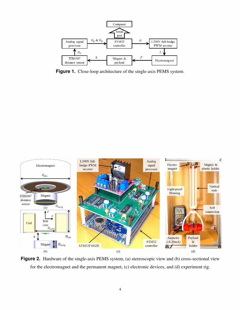
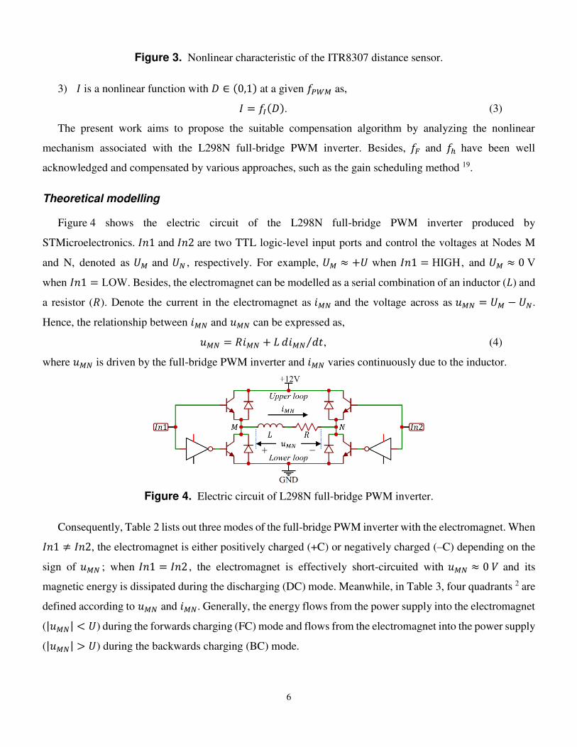
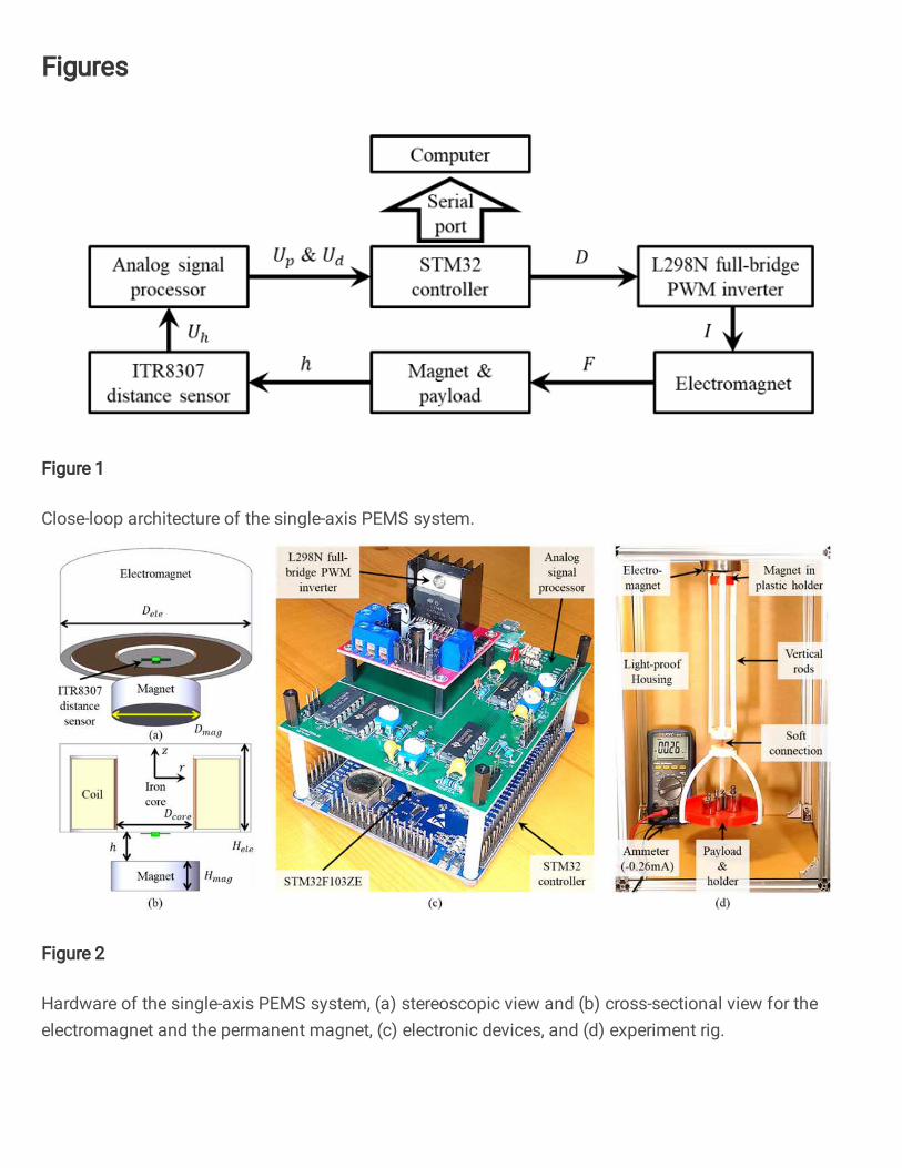
Figure 1 visualizes the close-loop architecture of the single-axis PEMS system, Figure 2 visualizes the

associated hardware, and Table 1 lists out physical properties. The six elements are:

1) Floater includes the payload and the Nd-Fe-B permanent magnet with the grade of N35. The magnet

holder keeps the minimum gap between the magnet and the iron core to protect the ITR8307 sensor, while

the three vertical rods and the soft connection maintains the upwards orientation of the magnet regardless of

the gravity center of the payload;

2) ITR8307 distance sensor converts the floating height (ℎ) between the floater and the electromagnet

into the height signal (𝑈ℎ) by the reflection intensity of the infra light. Besides, a light-proof housing is

installed to entirely cover the single-axis PEMS system;

3) Analog signal processor converts 𝑈ℎ into the proportional and differential signals (𝑈𝑝 and 𝑈𝑑);

4) Digital STM32 controller outputs the PWM signal with 𝑓𝑃𝑊𝑀 and 𝐷 (based on 𝑈𝑝, 𝑈𝑑 and the double-

loop control algorithm). Besides, the real-time data are upload to the computer by the serial port;

5) L298N full-bridge PWM inverter converts the PWM signal into 𝐼 through the electromagnet. 𝐼 is

measured by the ammeter, while the voltage across the electromagnet is measured by the oscilloscope; and

6) Electromagnet generates the attractive magnetic force (𝐹) on the magnet to balance the gravity (𝐺) of

the floater.

4

Figure 1. Close-loop architecture of the single-axis PEMS system.

Figure 2. Hardware of the single-axis PEMS system, (a) stereoscopic view and (b) cross-sectional view

for the electromagnet and the permanent magnet, (c) electronic devices, and (d) experiment rig.

5

Symbols Quantity Value Unit 𝑚 Floater mass 0.76 kg 𝑀 Electromagnet mass 0.59 kg 𝑅 Electromagnet resistor 14.5 Ω 𝑈 Power supply voltage 12 V 𝑓𝑃𝑊𝑀 PWM frequency 0.1~100 kHz 𝑓𝑐𝑟 Critical PWM frequency 15.28 kHz 𝑇 PWM period 0.01~10 ms 𝑓𝑠𝑎𝑚𝑝𝑙𝑒 Controller sampling rate 200 Hz 𝐷𝑚𝑎𝑔 Magnet diameter 30 mm 𝐻𝑚𝑎𝑔 Magnet thickness 10 mm 𝐷𝑒𝑙𝑒 Electromagnet outer diameter 65 mm 𝐷𝑐𝑜𝑟𝑒 Electromagnet iron-core diameter 26 mm 𝐻𝑒𝑙𝑒 Electromagnet thickness 30 mm ℎ Floating height 9.5~10.9 mm

Table 1. Physical properties of the single-axis PEMS system.

Moreover, there are three nonlinear relationships for the single-axis PEMS system in Fig. 1:

1) 𝐹 is a nonlinear function with ℎ and 𝐼 as, 𝐹 = 𝐹𝑝 + 𝐹𝑒 = 𝑓𝐹(ℎ, 𝐼), (1)

where 𝐹 has two components as,

(i) Permanent magnetic force (𝐹𝑝): 𝐹𝑝 is the attractive magnetic force between the permanent magnet and

the iron core of the electromagnet. And, 𝐹𝑝 is a nonlinear decreasing function of ℎ 19; and

(ii) Electromagnetic force ( 𝐹𝑒 ): 𝐹𝑒 is the magnetic force between the permanent magnet and the

electromagnet and is linear with 𝐼 8. As a sign conventional, 𝐼 > 0 leads to attractive 𝐹𝑒 , and vice

versa.

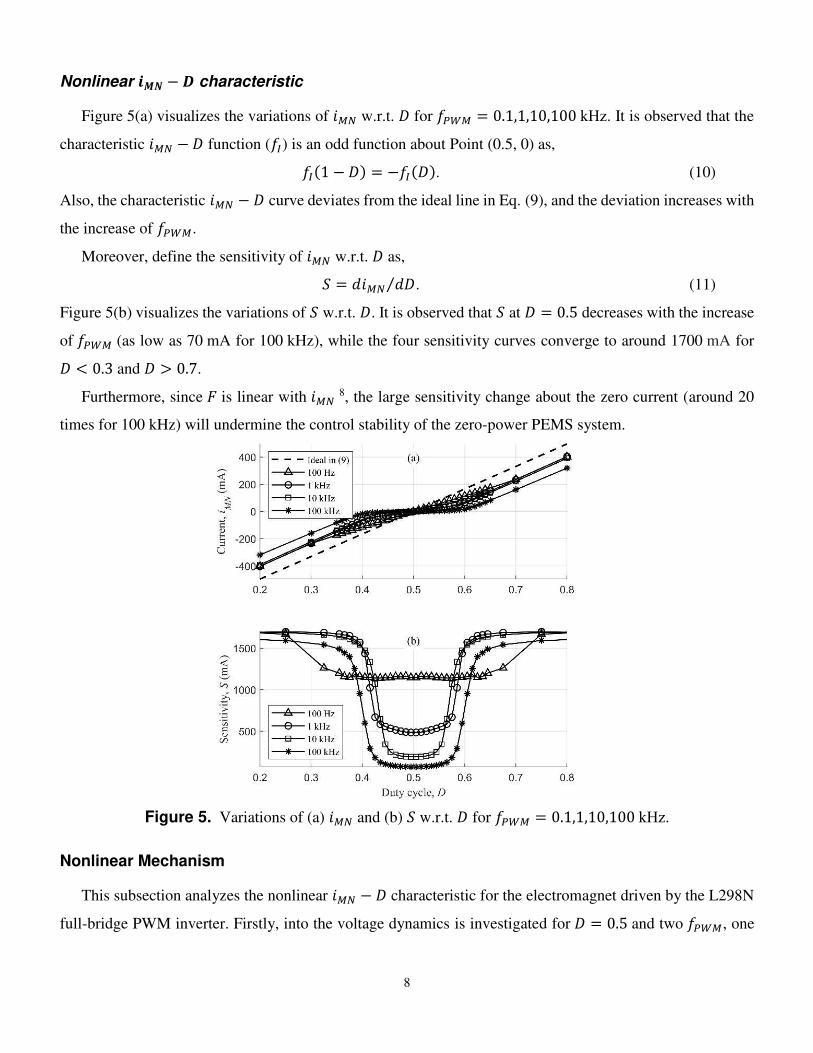
2) 𝑈ℎ is a nonlinear function with ℎ as, 𝑈ℎ = 𝑓ℎ(ℎ) ∈ (0, 3.3) V. (2)

Figure 3 visualizes the nonlinear characteristic of the ITR8307 distance sensor. It is observed that 𝑈ℎ is an

increasing function of ℎ with a decreasing slope.

6

Figure 3. Nonlinear characteristic of the ITR8307 distance sensor.

3) 𝐼 is a nonlinear function with 𝐷 ∈ (0,1) at a given 𝑓𝑃𝑊𝑀 as, 𝐼 = 𝑓𝐼(𝐷). (3)

The present work aims to propose the suitable compensation algorithm by analyzing the nonlinear

mechanism associated with the L298N full-bridge PWM inverter. Besides, 𝑓𝐹 and 𝑓ℎ have been well

acknowledged and compensated by various approaches, such as the gain scheduling method 19.

Theoretical modelling

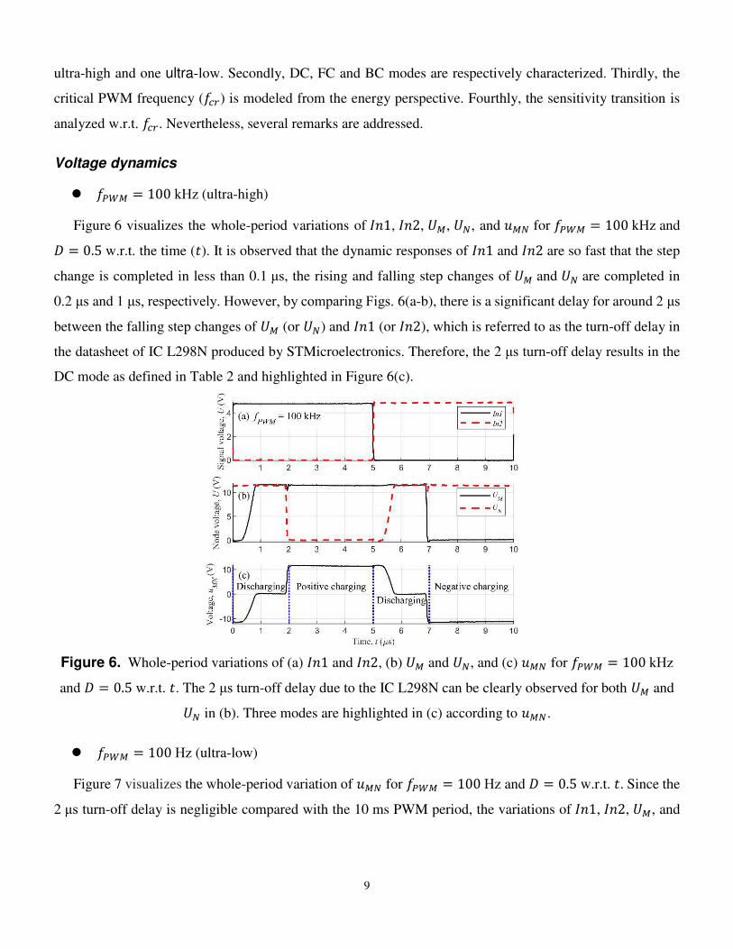
Figure 4 shows the electric circuit of the L298N full-bridge PWM inverter produced by

STMicroelectronics. 𝐼𝑛1 and 𝐼𝑛2 are two TTL logic-level input ports and control the voltages at Nodes M

and N, denoted as 𝑈𝑀 and 𝑈𝑁 , respectively. For example, 𝑈𝑀 ≈ +𝑈 when 𝐼𝑛1 = HIGH , and 𝑈𝑀 ≈ 0 V

when 𝐼𝑛1 = LOW. Besides, the electromagnet can be modelled as a serial combination of an inductor (𝐿) and

a resistor (𝑅). Denote the current in the electromagnet as 𝑖𝑀𝑁 and the voltage across as 𝑢𝑀𝑁 = 𝑈𝑀 − 𝑈𝑁.

Hence, the relationship between 𝑖𝑀𝑁 and 𝑢𝑀𝑁 can be expressed as, 𝑢𝑀𝑁 = 𝑅𝑖𝑀𝑁 + 𝐿 𝑑𝑖𝑀𝑁 𝑑𝑡⁄ , (4)

where 𝑢𝑀𝑁 is driven by the full-bridge PWM inverter and 𝑖𝑀𝑁 varies continuously due to the inductor.

Figure 4. Electric circuit of L298N full-bridge PWM inverter.

Consequently, Table 2 lists out three modes of the full-bridge PWM inverter with the electromagnet. When 𝐼𝑛1 ≠ 𝐼𝑛2, the electromagnet is either positively charged (+C) or negatively charged (–C) depending on the

sign of 𝑢𝑀𝑁 ; when 𝐼𝑛1 = 𝐼𝑛2 , the electromagnet is effectively short-circuited with 𝑢𝑀𝑁 ≈ 0 𝑉 and its

magnetic energy is dissipated during the discharging (DC) mode. Meanwhile, in Table 3, four quadrants 2 are

defined according to 𝑢𝑀𝑁 and 𝑖𝑀𝑁. Generally, the energy flows from the power supply into the electromagnet

(|𝑢𝑀𝑁| < 𝑈) during the forwards charging (FC) mode and flows from the electromagnet into the power supply

(|𝑢𝑀𝑁| > 𝑈) during the backwards charging (BC) mode.

7

𝐼𝑛1 = HIGH 𝐼𝑛1 = LOW 𝐼𝑛2 = HIGH DC: 𝑢𝑀𝑁 ≈ 0 𝑉. –C: 𝑢𝑀𝑁 ≈ −𝑈. 𝐼𝑛2 = LOW +C: 𝑢𝑀𝑁 ≈ +𝑈. DC: 𝑢𝑀𝑁 ≈ 0 𝑉.

Table 2. Three modes of full-bridge PWM inverter with electromagnet.

𝑢𝑀𝑁 ≈ −𝑈 𝑢𝑀𝑁 ≈ +𝑈 𝑖𝑀𝑁 > 0 (2nd quadrant) –BC: 𝑢𝑀𝑁 < −𝑈. (1st quadrant) +FC: 𝑢𝑀𝑁 < +𝑈. 𝑖𝑀𝑁 < 0 (3rd quadrant) –FC: 𝑢𝑀𝑁 > −𝑈. (4th quadrant) +BC: 𝑢𝑀𝑁 > +𝑈.

Table 3. Four quadrants of full-bridge PWM inverter with electromagnet.

In the present work, 𝐼𝑛1 is the PWM signal generated by the STM32 controller and 𝐼𝑛2 is obtained by the

NOT gate as, 𝐼𝑛1 = 𝑃𝑊𝑀 and 𝐼𝑛2 = 𝑃𝑊𝑀̅̅ ̅̅ ̅̅ ̅, (5)

where the PWM signal can be explicitly expressed as, 𝑃𝑊𝑀 = {HIGH, 𝑛𝑇 < 𝑡 < (𝑛 + 𝐷)𝑇LOW, (𝑛 + 𝐷)𝑇 < 𝑡 < (𝑛 + 1)𝑇, (6)

where 𝑇 (= 1 𝑓𝑃𝑊𝑀⁄ ) denotes the period of the PWM signal and 𝑛 is any arbitrary integer.

Assuming the ideal full-bridge PWM inverter, 𝑢𝑀𝑁 can be expressed by referring to Table 2 and Eqs. (5-

6) as, 𝑢𝑀𝑁 = {+𝑈, 𝑛𝑇 < 𝑡 < (𝑛 + 𝐷)𝑇−𝑈, (𝑛 + 𝐷)𝑇 < 𝑡 < (𝑛 + 1)𝑇. (7)

Moreover, denote the equilibrium current at 𝑡 = 𝑛𝑇 as 𝐼1 and that at 𝑡 = (𝑛 + 𝐷)𝑇 as 𝐼2. Solving Eq. (4)

together with Eq. (7) gives the two equilibrium currents as,

{𝐼1 = 𝑈𝑅 (𝑒−𝑅𝑇𝐿 + 1 − 2𝑒−(1−𝐷)𝑅𝑇𝐿 ) (𝑒−𝑅𝑇𝐿 − 1)⁄𝐼2 = 𝑈𝑅 (2𝑒−𝐷𝑅𝑇𝐿 − 𝑒−𝑅𝑇𝐿 − 1) (𝑒−𝑅𝑇𝐿 − 1)⁄ , (8)

which indicates that 𝑖𝑀𝑁 fluctuates between 𝐼1 and 𝐼2. Since the time constant of the electromagnet (𝐿 𝑅⁄ ≈5 to 9 ms to be fully charged or discharged in Fig. 9) is much larger than the PWM period (e.g., 𝑇 = 0.1 ms

for 10 kHz), i.e., 𝑅𝑇 𝐿⁄ ≪ 1, Eq. (8) can be approximated as, 𝑖𝑀𝑁 ≈ 𝐼1 ≈ 𝐼2 ≈ 𝑈𝑅 (2𝐷 − 1) ∈ [−𝑈 𝑅⁄ , 𝑈 𝑅⁄ ], (9)

which indicates that ideal 𝑖𝑀𝑁 in the electromagnet is linear with the duty cycle under a high 𝑓𝑃𝑊𝑀.

8

Nonlinear 𝒊𝑴𝑵 −𝑫 characteristic

Figure 5(a) visualizes the variations of 𝑖𝑀𝑁 w.r.t. 𝐷 for 𝑓𝑃𝑊𝑀 = 0.1,1,10,100 kHz. It is observed that the

characteristic 𝑖𝑀𝑁 −𝐷 function (𝑓𝐼) is an odd function about Point (0.5, 0) as, 𝑓𝐼(1 − 𝐷) = −𝑓𝐼(𝐷). (10)

Also, the characteristic 𝑖𝑀𝑁 − 𝐷 curve deviates from the ideal line in Eq. (9), and the deviation increases with

the increase of 𝑓𝑃𝑊𝑀.

Moreover, define the sensitivity of 𝑖𝑀𝑁 w.r.t. 𝐷 as, 𝑆 = 𝑑𝑖𝑀𝑁 𝑑𝐷⁄ . (11)

Figure 5(b) visualizes the variations of 𝑆 w.r.t. 𝐷. It is observed that 𝑆 at 𝐷 = 0.5 decreases with the increase

of 𝑓𝑃𝑊𝑀 (as low as 70 mA for 100 kHz), while the four sensitivity curves converge to around 1700 mA for 𝐷 < 0.3 and 𝐷 > 0.7.

Furthermore, since 𝐹 is linear with 𝑖𝑀𝑁 8, the large sensitivity change about the zero current (around 20

times for 100 kHz) will undermine the control stability of the zero-power PEMS system.

Figure 5. Variations of (a) 𝑖𝑀𝑁 and (b) 𝑆 w.r.t. 𝐷 for 𝑓𝑃𝑊𝑀 = 0.1,1,10,100 kHz.

Nonlinear Mechanism

This subsection analyzes the nonlinear 𝑖𝑀𝑁 − 𝐷 characteristic for the electromagnet driven by the L298N

full-bridge PWM inverter. Firstly, into the voltage dynamics is investigated for 𝐷 = 0.5 and two 𝑓𝑃𝑊𝑀, one

9

ultra-high and one ultra-low. Secondly, DC, FC and BC modes are respectively characterized. Thirdly, the

critical PWM frequency (𝑓𝑐𝑟) is modeled from the energy perspective. Fourthly, the sensitivity transition is

analyzed w.r.t. 𝑓𝑐𝑟. Nevertheless, several remarks are addressed.

Voltage dynamics

𝑓𝑃𝑊𝑀 = 100 kHz (ultra-high)

Figure 6 visualizes the whole-period variations of 𝐼𝑛1, 𝐼𝑛2, 𝑈𝑀, 𝑈𝑁, and 𝑢𝑀𝑁 for 𝑓𝑃𝑊𝑀 = 100 kHz and 𝐷 = 0.5 w.r.t. the time (𝑡). It is observed that the dynamic responses of 𝐼𝑛1 and 𝐼𝑛2 are so fast that the step

change is completed in less than 0.1 μs, the rising and falling step changes of 𝑈𝑀 and 𝑈𝑁 are completed in

0.2 μs and 1 μs, respectively. However, by comparing Figs. 6(a-b), there is a significant delay for around 2 μs

between the falling step changes of 𝑈𝑀 (or 𝑈𝑁) and 𝐼𝑛1 (or 𝐼𝑛2), which is referred to as the turn-off delay in

the datasheet of IC L298N produced by STMicroelectronics. Therefore, the 2 μs turn-off delay results in the

DC mode as defined in Table 2 and highlighted in Figure 6(c).

Figure 6. Whole-period variations of (a) 𝐼𝑛1 and 𝐼𝑛2, (b) 𝑈𝑀 and 𝑈𝑁, and (c) 𝑢𝑀𝑁 for 𝑓𝑃𝑊𝑀 = 100 kHz

and 𝐷 = 0.5 w.r.t. 𝑡. The 2 μs turn-off delay due to the IC L298N can be clearly observed for both 𝑈𝑀 and 𝑈𝑁 in (b). Three modes are highlighted in (c) according to 𝑢𝑀𝑁.

𝑓𝑃𝑊𝑀 = 100 Hz (ultra-low)

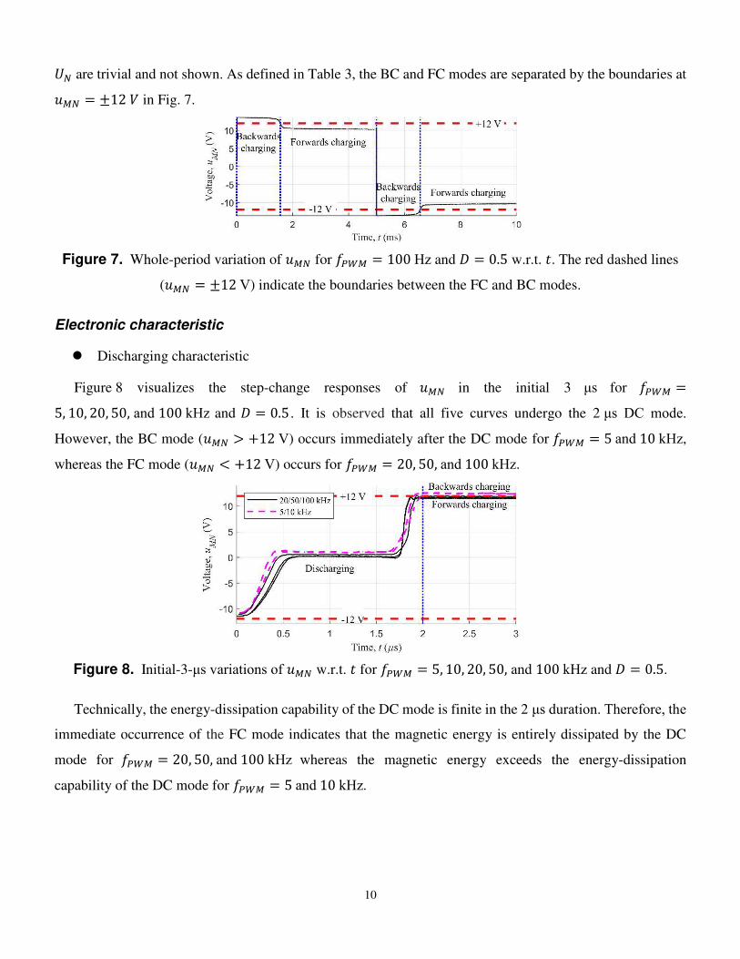
Figure 7 visualizes the whole-period variation of 𝑢𝑀𝑁 for 𝑓𝑃𝑊𝑀 = 100 Hz and 𝐷 = 0.5 w.r.t. 𝑡. Since the

2 μs turn-off delay is negligible compared with the 10 ms PWM period, the variations of 𝐼𝑛1, 𝐼𝑛2, 𝑈𝑀, and

10

𝑈𝑁 are trivial and not shown. As defined in Table 3, the BC and FC modes are separated by the boundaries at 𝑢𝑀𝑁 = ±12 𝑉 in Fig. 7.

Figure 7. Whole-period variation of 𝑢𝑀𝑁 for 𝑓𝑃𝑊𝑀 = 100 Hz and 𝐷 = 0.5 w.r.t. 𝑡. The red dashed lines

(𝑢𝑀𝑁 = ±12 V) indicate the boundaries between the FC and BC modes.

Electronic characteristic

Discharging characteristic

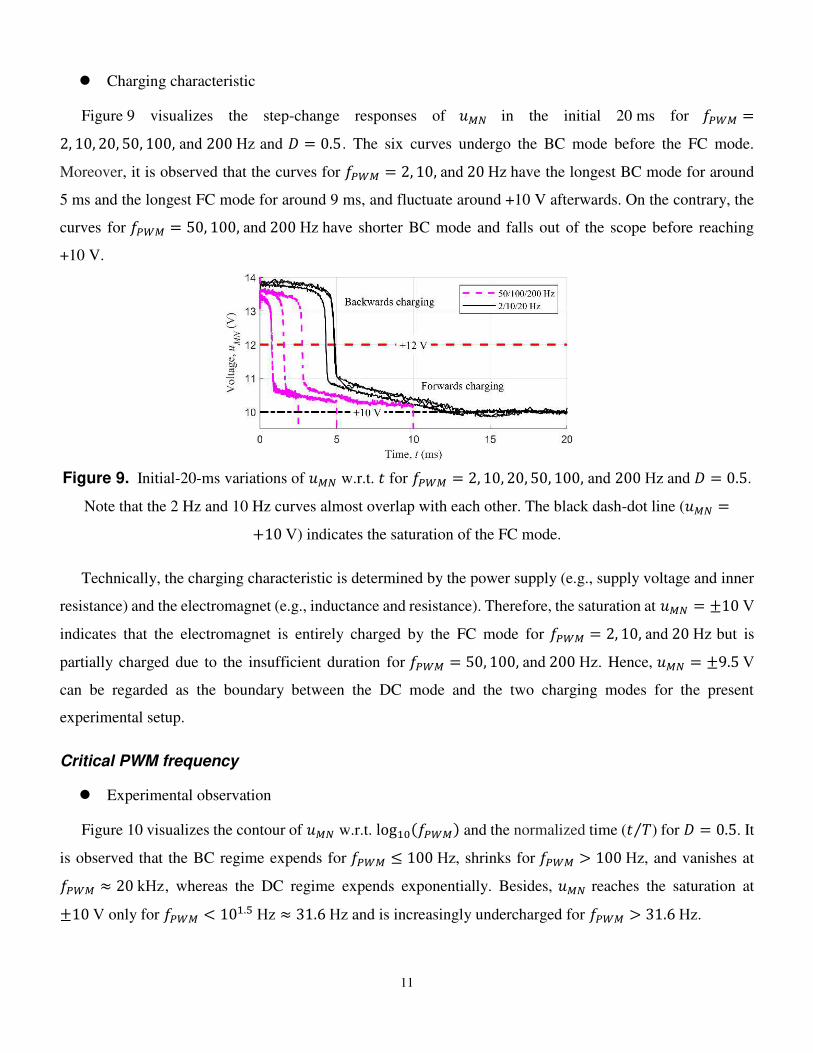
Figure 8 visualizes the step-change responses of 𝑢𝑀𝑁 in the initial 3 μs for 𝑓𝑃𝑊𝑀 =5, 10, 20, 50, and 100 kHz and 𝐷 = 0.5 . It is observed that all five curves undergo the 2 μs DC mode.

However, the BC mode (𝑢𝑀𝑁 > +12 V) occurs immediately after the DC mode for 𝑓𝑃𝑊𝑀 = 5 and 10 kHz,

whereas the FC mode (𝑢𝑀𝑁 < +12 V) occurs for 𝑓𝑃𝑊𝑀 = 20, 50, and 100 kHz.

Figure 8. Initial-3-μs variations of 𝑢𝑀𝑁 w.r.t. 𝑡 for 𝑓𝑃𝑊𝑀 = 5, 10, 20, 50, and 100 kHz and 𝐷 = 0.5.

Technically, the energy-dissipation capability of the DC mode is finite in the 2 μs duration. Therefore, the

immediate occurrence of the FC mode indicates that the magnetic energy is entirely dissipated by the DC

mode for 𝑓𝑃𝑊𝑀 = 20, 50, and 100 kHz whereas the magnetic energy exceeds the energy-dissipation

capability of the DC mode for 𝑓𝑃𝑊𝑀 = 5 and 10 kHz.

11

Charging characteristic

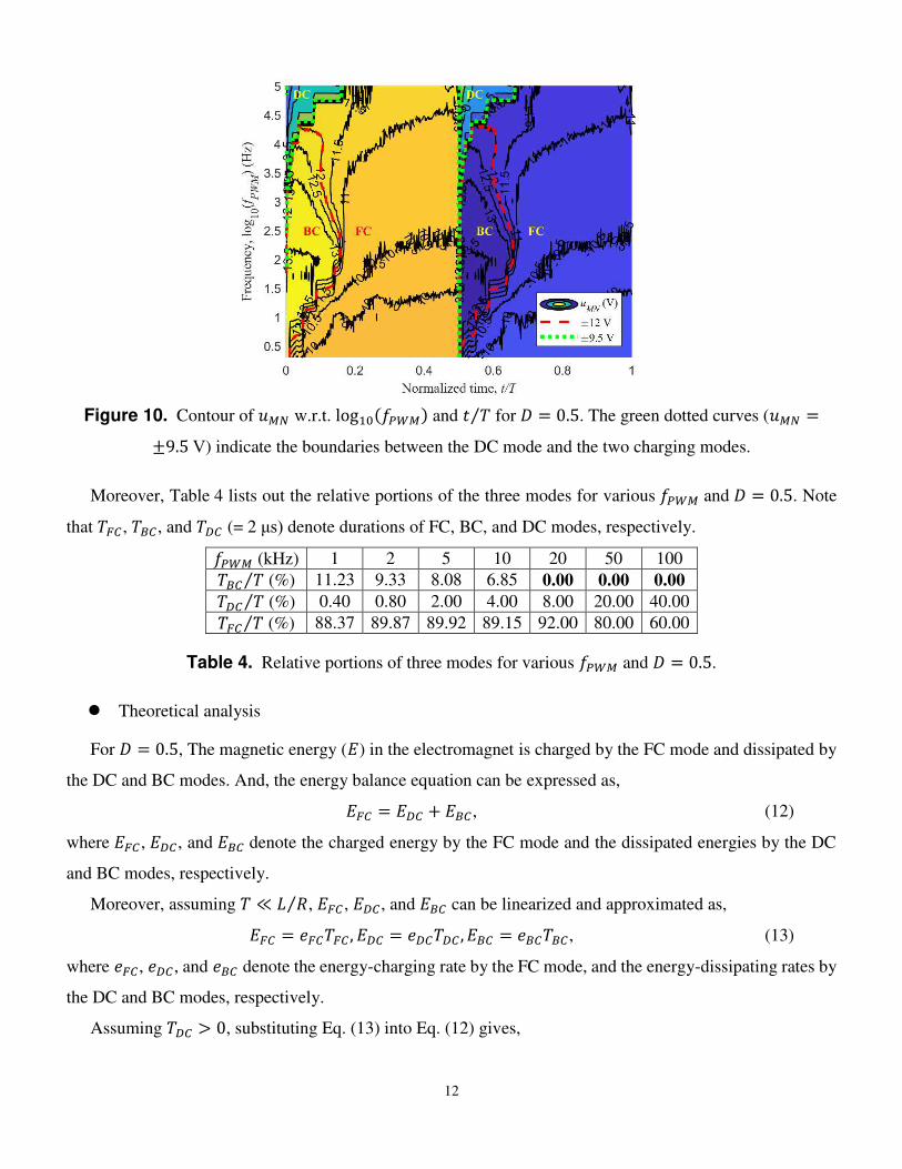
Figure 9 visualizes the step-change responses of 𝑢𝑀𝑁 in the initial 20 ms for 𝑓𝑃𝑊𝑀 =2, 10, 20, 50, 100, and 200 Hz and 𝐷 = 0.5. The six curves undergo the BC mode before the FC mode.

Moreover, it is observed that the curves for 𝑓𝑃𝑊𝑀 = 2, 10, and 20 Hz have the longest BC mode for around

5 ms and the longest FC mode for around 9 ms, and fluctuate around +10 V afterwards. On the contrary, the

curves for 𝑓𝑃𝑊𝑀 = 50, 100, and 200 Hz have shorter BC mode and falls out of the scope before reaching

+10 V.

Figure 9. Initial-20-ms variations of 𝑢𝑀𝑁 w.r.t. 𝑡 for 𝑓𝑃𝑊𝑀 = 2, 10, 20, 50, 100, and 200 Hz and 𝐷 = 0.5.

Note that the 2 Hz and 10 Hz curves almost overlap with each other. The black dash-dot line (𝑢𝑀𝑁 =+10 V) indicates the saturation of the FC mode.

Technically, the charging characteristic is determined by the power supply (e.g., supply voltage and inner

resistance) and the electromagnet (e.g., inductance and resistance). Therefore, the saturation at 𝑢𝑀𝑁 = ±10 V

indicates that the electromagnet is entirely charged by the FC mode for 𝑓𝑃𝑊𝑀 = 2, 10, and 20 Hz but is

partially charged due to the insufficient duration for 𝑓𝑃𝑊𝑀 = 50, 100, and 200 Hz. Hence, 𝑢𝑀𝑁 = ±9.5 V

can be regarded as the boundary between the DC mode and the two charging modes for the present

experimental setup.

Critical PWM frequency

Experimental observation

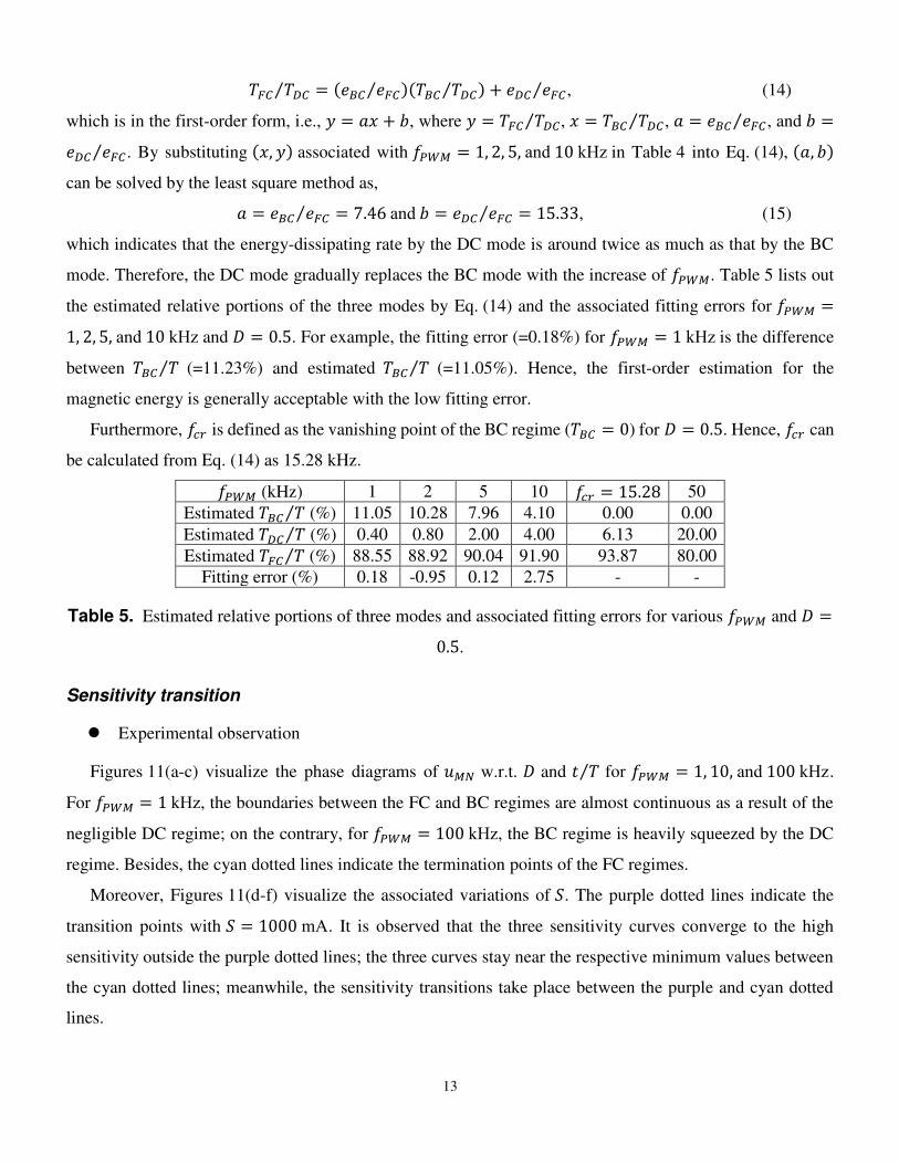
Figure 10 visualizes the contour of 𝑢𝑀𝑁 w.r.t. log10(𝑓𝑃𝑊𝑀) and the normalized time (𝑡 𝑇⁄ ) for 𝐷 = 0.5. It

is observed that the BC regime expends for 𝑓𝑃𝑊𝑀 ≤ 100 Hz, shrinks for 𝑓𝑃𝑊𝑀 > 100 Hz, and vanishes at 𝑓𝑃𝑊𝑀 ≈ 20 kHz, whereas the DC regime expends exponentially. Besides, 𝑢𝑀𝑁 reaches the saturation at ±10 V only for 𝑓𝑃𝑊𝑀 < 101.5 Hz ≈ 31.6 Hz and is increasingly undercharged for 𝑓𝑃𝑊𝑀 > 31.6 Hz.

12

Figure 10. Contour of 𝑢𝑀𝑁 w.r.t. log10(𝑓𝑃𝑊𝑀) and 𝑡 𝑇⁄ for 𝐷 = 0.5. The green dotted curves (𝑢𝑀𝑁 =±9.5 V) indicate the boundaries between the DC mode and the two charging modes.

Moreover, Table 4 lists out the relative portions of the three modes for various 𝑓𝑃𝑊𝑀 and 𝐷 = 0.5. Note

that 𝑇𝐹𝐶, 𝑇𝐵𝐶, and 𝑇𝐷𝐶 (= 2 μs) denote durations of FC, BC, and DC modes, respectively. 𝑓𝑃𝑊𝑀 (kHz) 1 2 5 10 20 50 100 𝑇𝐵𝐶 𝑇⁄ (%) 11.23 9.33 8.08 6.85 0.00 0.00 0.00 𝑇𝐷𝐶 𝑇⁄ (%) 0.40 0.80 2.00 4.00 8.00 20.00 40.00 𝑇𝐹𝐶 𝑇⁄ (%) 88.37 89.87 89.92 89.15 92.00 80.00 60.00

Table 4. Relative portions of three modes for various 𝑓𝑃𝑊𝑀 and 𝐷 = 0.5.

Theoretical analysis

For 𝐷 = 0.5, The magnetic energy (𝐸) in the electromagnet is charged by the FC mode and dissipated by

the DC and BC modes. And, the energy balance equation can be expressed as, 𝐸𝐹𝐶 = 𝐸𝐷𝐶 + 𝐸𝐵𝐶, (12)

where 𝐸𝐹𝐶 , 𝐸𝐷𝐶, and 𝐸𝐵𝐶 denote the charged energy by the FC mode and the dissipated energies by the DC

and BC modes, respectively.

Moreover, assuming 𝑇 ≪ 𝐿 𝑅⁄ , 𝐸𝐹𝐶 , 𝐸𝐷𝐶, and 𝐸𝐵𝐶 can be linearized and approximated as, 𝐸𝐹𝐶 = 𝑒𝐹𝐶𝑇𝐹𝐶 , 𝐸𝐷𝐶 = 𝑒𝐷𝐶𝑇𝐷𝐶 , 𝐸𝐵𝐶 = 𝑒𝐵𝐶𝑇𝐵𝐶, (13)

where 𝑒𝐹𝐶, 𝑒𝐷𝐶, and 𝑒𝐵𝐶 denote the energy-charging rate by the FC mode, and the energy-dissipating rates by

the DC and BC modes, respectively.

Assuming 𝑇𝐷𝐶 > 0, substituting Eq. (13) into Eq. (12) gives,

13

𝑇𝐹𝐶 𝑇𝐷𝐶⁄ = (𝑒𝐵𝐶 𝑒𝐹𝐶⁄ )(𝑇𝐵𝐶 𝑇𝐷𝐶⁄ ) + 𝑒𝐷𝐶 𝑒𝐹𝐶⁄ , (14)

which is in the first-order form, i.e., 𝑦 = 𝑎𝑥 + 𝑏, where 𝑦 = 𝑇𝐹𝐶 𝑇𝐷𝐶⁄ , 𝑥 = 𝑇𝐵𝐶 𝑇𝐷𝐶⁄ , 𝑎 = 𝑒𝐵𝐶 𝑒𝐹𝐶⁄ , and 𝑏 =𝑒𝐷𝐶 𝑒𝐹𝐶⁄ . By substituting (𝑥, 𝑦) associated with 𝑓𝑃𝑊𝑀 = 1, 2, 5, and 10 kHz in Table 4 into Eq. (14), (𝑎, 𝑏) can be solved by the least square method as, 𝑎 = 𝑒𝐵𝐶 𝑒𝐹𝐶⁄ = 7.46 and 𝑏 = 𝑒𝐷𝐶 𝑒𝐹𝐶⁄ = 15.33, (15)

which indicates that the energy-dissipating rate by the DC mode is around twice as much as that by the BC

mode. Therefore, the DC mode gradually replaces the BC mode with the increase of 𝑓𝑃𝑊𝑀. Table 5 lists out

the estimated relative portions of the three modes by Eq. (14) and the associated fitting errors for 𝑓𝑃𝑊𝑀 =1, 2, 5, and 10 kHz and 𝐷 = 0.5. For example, the fitting error (=0.18%) for 𝑓𝑃𝑊𝑀 = 1 kHz is the difference

between 𝑇𝐵𝐶 𝑇⁄ (=11.23%) and estimated 𝑇𝐵𝐶 𝑇⁄ (=11.05%). Hence, the first-order estimation for the

magnetic energy is generally acceptable with the low fitting error.

Furthermore, 𝑓𝑐𝑟 is defined as the vanishing point of the BC regime (𝑇𝐵𝐶 = 0) for 𝐷 = 0.5. Hence, 𝑓𝑐𝑟 can

be calculated from Eq. (14) as 15.28 kHz. 𝑓𝑃𝑊𝑀 (kHz) 1 2 5 10 𝑓𝑐𝑟 = 15.28 50

Estimated 𝑇𝐵𝐶 𝑇⁄ (%) 11.05 10.28 7.96 4.10 0.00 0.00

Estimated 𝑇𝐷𝐶 𝑇⁄ (%) 0.40 0.80 2.00 4.00 6.13 20.00

Estimated 𝑇𝐹𝐶 𝑇⁄ (%) 88.55 88.92 90.04 91.90 93.87 80.00

Fitting error (%) 0.18 -0.95 0.12 2.75 - -

Table 5. Estimated relative portions of three modes and associated fitting errors for various 𝑓𝑃𝑊𝑀 and 𝐷 =0.5.

Sensitivity transition

Experimental observation

Figures 11(a-c) visualize the phase diagrams of 𝑢𝑀𝑁 w.r.t. 𝐷 and 𝑡 𝑇⁄ for 𝑓𝑃𝑊𝑀 = 1, 10, and 100 kHz.

For 𝑓𝑃𝑊𝑀 = 1 kHz, the boundaries between the FC and BC regimes are almost continuous as a result of the

negligible DC regime; on the contrary, for 𝑓𝑃𝑊𝑀 = 100 kHz, the BC regime is heavily squeezed by the DC

regime. Besides, the cyan dotted lines indicate the termination points of the FC regimes.

Moreover, Figures 11(d-f) visualize the associated variations of 𝑆. The purple dotted lines indicate the

transition points with 𝑆 = 1000 mA. It is observed that the three sensitivity curves converge to the high

sensitivity outside the purple dotted lines; the three curves stay near the respective minimum values between

the cyan dotted lines; meanwhile, the sensitivity transitions take place between the purple and cyan dotted

lines.

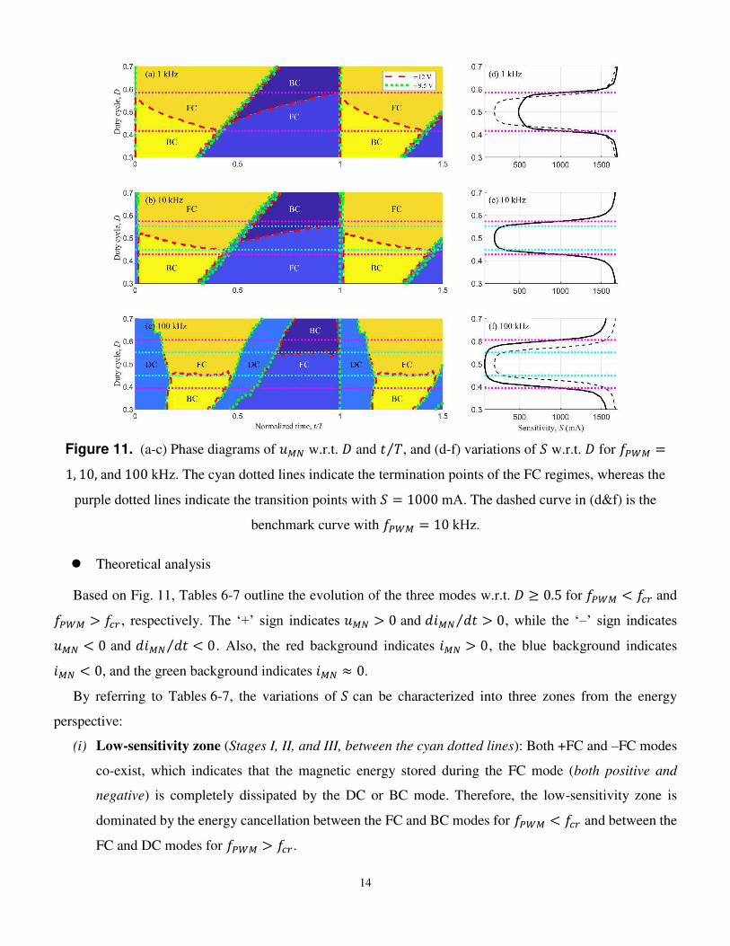
14

Figure 11. (a-c) Phase diagrams of 𝑢𝑀𝑁 w.r.t. 𝐷 and 𝑡 𝑇⁄ , and (d-f) variations of 𝑆 w.r.t. 𝐷 for 𝑓𝑃𝑊𝑀 =1, 10, and 100 kHz. The cyan dotted lines indicate the termination points of the FC regimes, whereas the

purple dotted lines indicate the transition points with 𝑆 = 1000 mA. The dashed curve in (d&f) is the

benchmark curve with 𝑓𝑃𝑊𝑀 = 10 kHz.

Theoretical analysis

Based on Fig. 11, Tables 6-7 outline the evolution of the three modes w.r.t. 𝐷 ≥ 0.5 for 𝑓𝑃𝑊𝑀 < 𝑓𝑐𝑟 and 𝑓𝑃𝑊𝑀 > 𝑓𝑐𝑟 , respectively. The ‘+’ sign indicates 𝑢𝑀𝑁 > 0 and 𝑑𝑖𝑀𝑁 𝑑𝑡⁄ > 0, while the ‘–’ sign indicates 𝑢𝑀𝑁 < 0 and 𝑑𝑖𝑀𝑁 𝑑𝑡⁄ < 0. Also, the red background indicates 𝑖𝑀𝑁 > 0, the blue background indicates 𝑖𝑀𝑁 < 0, and the green background indicates 𝑖𝑀𝑁 ≈ 0.

By referring to Tables 6-7, the variations of 𝑆 can be characterized into three zones from the energy

perspective:

(i) Low-sensitivity zone (Stages I, II, and III, between the cyan dotted lines): Both +FC and –FC modes

co-exist, which indicates that the magnetic energy stored during the FC mode (both positive and

negative) is completely dissipated by the DC or BC mode. Therefore, the low-sensitivity zone is

dominated by the energy cancellation between the FC and BC modes for 𝑓𝑃𝑊𝑀 < 𝑓𝑐𝑟 and between the

FC and DC modes for 𝑓𝑃𝑊𝑀 > 𝑓𝑐𝑟.

15

(ii) Sensitivity-transition zone (Stage IV, between the purple and cyan dotted lines): The 2 μs DC mode

has a finite energy-dissipation capability and buffers the sensitivity transition until the capability is

entirely consumed, as outlined by the purple and cyan dotted lines. Therefore, the sensitivity transition

expends with the increase of 𝑓𝑃𝑊𝑀.

(iii) High-sensitivity zone (Stage V, outside the purple dotted lines): The expending of the FC regime and

the shrinking of the BC regime occur simultaneously with the increase of the duty cycle. Therefore,

the magnetic energy accumulates more effectively in the high-sensitivity zone than that in the low-

sensitivity zone.

Stage 𝐷𝑇 (1 − 𝐷)𝑇 Zone

V –DC +FC –DC –BC High sensitivity

IV DC +FC –DC –BC Sensitivity transition

III DC +FC –DC –BC –FC

Low sensitivity II +DC +FC –DC –BC –FC

I (𝐷 ≈ 0.5) +DC +BC +FC –DC –BC –FC

Table 6. Evolution of three modes w.r.t. 𝐷 ≥ 0.5 for 𝑓𝑃𝑊𝑀 < 𝑓𝑐𝑟.

Stage 𝐷𝑇 (1 − 𝐷)𝑇 Zone

V –DC +FC –DC –BC High sensitivity

IV DC +FC –DC –BC Sensitivity transition

III DC +FC –DC –BC –FC

Low sensitivity II DC +FC –DC –FC

I (𝐷 ≈ 0.5) DC +FC DC –FC

Table 7. Evolution of three modes w.r.t. 𝐷 ≥ 0.5 for 𝑓𝑃𝑊𝑀 > 𝑓𝑐𝑟.

Remarks

This subsection investigates into the nonlinear mechanism of the 𝑖𝑀𝑁 − 𝐷 characteristic. The experimental

results indicate the following remarks:

1) In micro level, it is observed that the IC L298N possesses a 2 μs turn-off delay that leads to the passive

DC mode; in macro level, such a tiny delay results in the nonlinear 𝑖𝑀𝑁 − 𝐷 characteristic.

2) With the increase of 𝑓𝑃𝑊𝑀, the relative portion of the 2 μs DC mode is significantly amplified and

replaces the BC mode entirely at 𝐷 = 0.5 and 𝑓𝑐𝑟 = 15.28 kHz, which is theoretically modelled from the

energy perspective.

3) The low-sensitivity zone is dominated by the energy cancellation between the FC and BC modes for 𝑓𝑃𝑊𝑀 < 𝑓𝑐𝑟 and by the energy cancellation between the FC mode and the 2 μs DC mode for 𝑓𝑃𝑊𝑀 > 𝑓𝑐𝑟.

16

4) The sensitivity transition results from the finite energy-dissipation capability of the 2 μs DC mode and

expends with the increase of 𝑓𝑃𝑊𝑀.

5) Though higher 𝑓𝑃𝑊𝑀 can enhance the dynamic performance of the high-speed PEMS transportation

system 15, suitable compensation algorithm is necessary to take care of the nonlinear 𝑖𝑀𝑁 − 𝐷 characteristic

especially for 𝑓𝑃𝑊𝑀 > 𝑓𝑐𝑟. Compensation algorithm

Since 𝐹 is linear with 𝑖𝑀𝑁 8, this subsection proposes two piecewise linearization approaches to

approximate the nonlinear 𝑖𝑀𝑁 − 𝐷 characteristic with the full-bridge PWM inverter. The compensation

algorithm is verified by the current-step-change test over the sensitivity transition under two 𝑓𝑃𝑊𝑀 w.r.t. 𝑓𝑐𝑟.

For 𝒇𝑷𝑾𝑴 = 𝟏𝟎 kHz < 𝒇𝒄𝒓 Piecewise Linearization

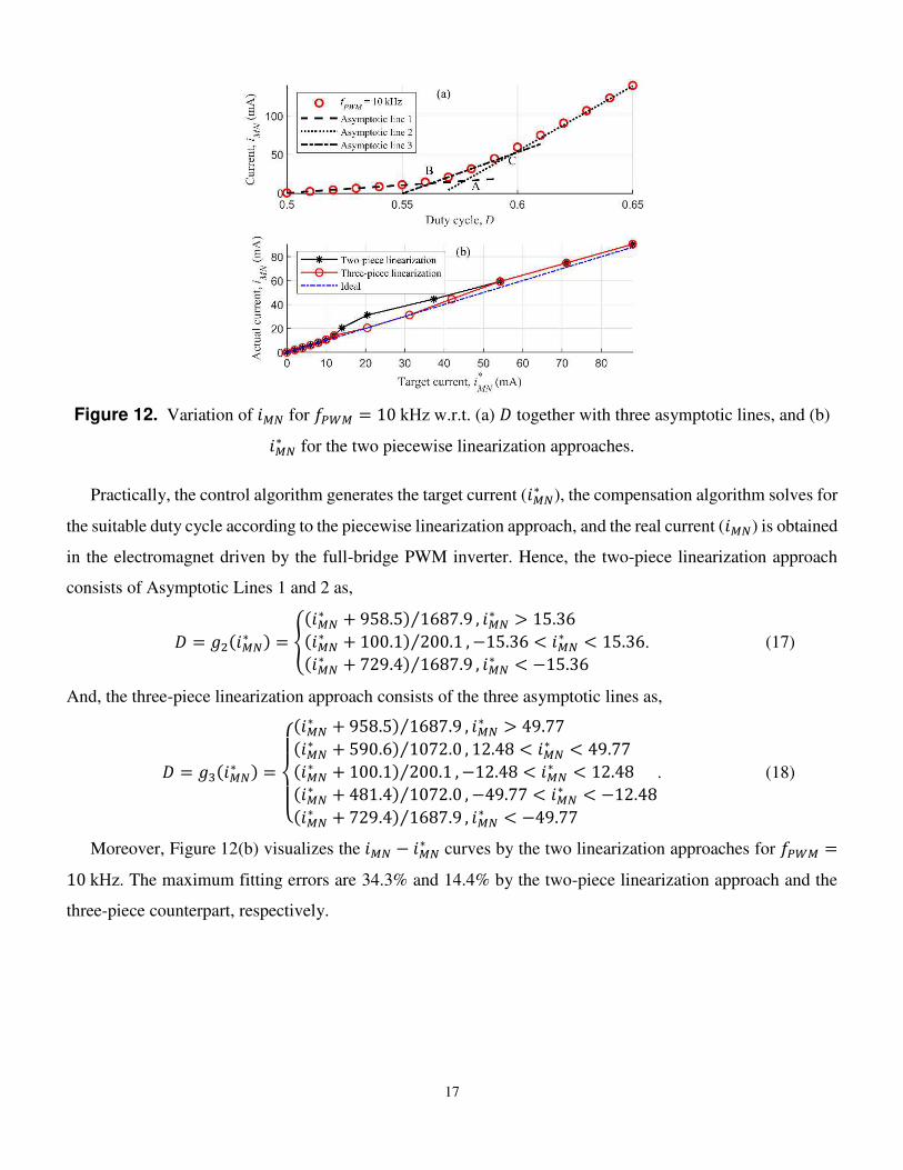
Figure 12(a) visualizes the nonlinear 𝑖𝑀𝑁 − 𝐷 characteristic for 𝑓𝑃𝑊𝑀 = 10 kHz < 𝑓𝑐𝑟 together with three

asymptotic lines. Asymptotic Line 1 is obtained by the two points at 𝐷 = 0.50 and 0.51, Asymptotic Line 2

is obtained by the two points at 𝐷 = 0.65 and 0.70, while Asymptotic Line 3 is obtained by the two points at 𝐷 = 0.57 and 0.58. The numerical expressions of the three asymptotic lines are,

{𝑖𝑀𝑁(1) = 𝑓𝐼(1)(𝐷) = 200.1𝐷 − 100.1𝑖𝑀𝑁(2) = 𝑓𝐼(2)(𝐷) = 1687.9𝐷 − 958.5𝑖𝑀𝑁(3) = 𝑓𝐼(3)(𝐷) = 1072.0𝐷 − 590.6. (16)

Note that the sensitivity ratio between 𝑓𝐼(1) and 𝑓𝐼(2) is more than 8 times, which will undermine the control

stability of the single-axis PEMS system over the medium sensitivity transition of the nonlinear 𝑖𝑀𝑁 − 𝐷

characteristic. Besides, the three intersection points among the three asymptotic lines are highlighted in

Fig. 12(a), including 𝐴 = (0.5770, 15.36 mA), 𝐵 = (0.5626, 12.48 mA), and 𝐶 = (0.5974, 49.77 mA).

17

Figure 12. Variation of 𝑖𝑀𝑁 for 𝑓𝑃𝑊𝑀 = 10 kHz w.r.t. (a) 𝐷 together with three asymptotic lines, and (b) 𝑖𝑀𝑁∗ for the two piecewise linearization approaches.

Practically, the control algorithm generates the target current (𝑖𝑀𝑁∗ ), the compensation algorithm solves for

the suitable duty cycle according to the piecewise linearization approach, and the real current (𝑖𝑀𝑁) is obtained

in the electromagnet driven by the full-bridge PWM inverter. Hence, the two-piece linearization approach

consists of Asymptotic Lines 1 and 2 as,

𝐷 = 𝑔2(𝑖𝑀𝑁∗ ) = {(𝑖𝑀𝑁∗ + 958.5) 1687.9⁄ , 𝑖𝑀𝑁∗ > 15.36(𝑖𝑀𝑁∗ + 100.1) 200.1⁄ , −15.36 < 𝑖𝑀𝑁∗ < 15.36(𝑖𝑀𝑁∗ + 729.4) 1687.9⁄ , 𝑖𝑀𝑁∗ < −15.36 . (17)

And, the three-piece linearization approach consists of the three asymptotic lines as,

𝐷 = 𝑔3(𝑖𝑀𝑁∗ ) = { (𝑖𝑀𝑁∗ + 958.5) 1687.9⁄ , 𝑖𝑀𝑁∗ > 49.77(𝑖𝑀𝑁∗ + 590.6) 1072.0⁄ , 12.48 < 𝑖𝑀𝑁∗ < 49.77(𝑖𝑀𝑁∗ + 100.1) 200.1⁄ ,−12.48 < 𝑖𝑀𝑁∗ < 12.48(𝑖𝑀𝑁∗ + 481.4) 1072.0⁄ , −49.77 < 𝑖𝑀𝑁∗ < −12.48(𝑖𝑀𝑁∗ + 729.4) 1687.9⁄ , 𝑖𝑀𝑁∗ < −49.77 . (18)

Moreover, Figure 12(b) visualizes the 𝑖𝑀𝑁 − 𝑖𝑀𝑁∗ curves by the two linearization approaches for 𝑓𝑃𝑊𝑀 =10 kHz. The maximum fitting errors are 34.3% and 14.4% by the two-piece linearization approach and the

three-piece counterpart, respectively.

18

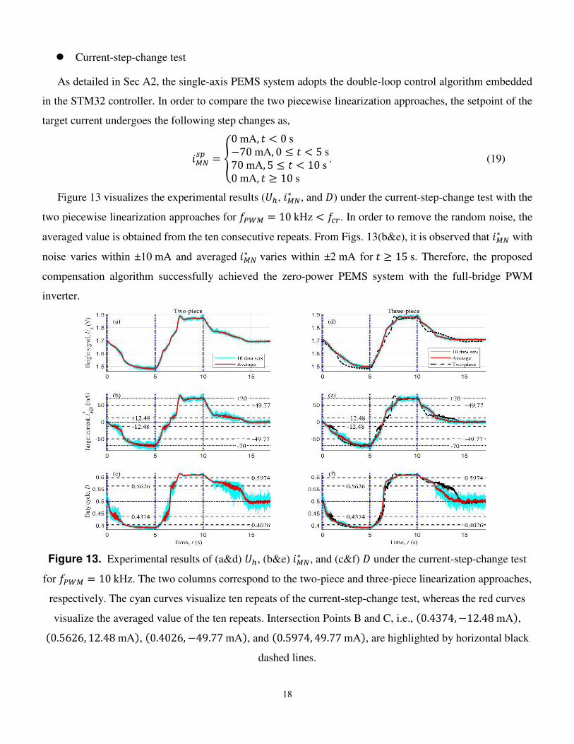
Current-step-change test

As detailed in Sec A2, the single-axis PEMS system adopts the double-loop control algorithm embedded

in the STM32 controller. In order to compare the two piecewise linearization approaches, the setpoint of the

target current undergoes the following step changes as,

𝑖𝑀𝑁𝑠𝑝 = {0 mA, 𝑡 < 0 s−70 mA, 0 ≤ 𝑡 < 5 s70 mA, 5 ≤ 𝑡 < 10 s0 mA, 𝑡 ≥ 10 s . (19)

Figure 13 visualizes the experimental results (𝑈ℎ, 𝑖𝑀𝑁∗ , and 𝐷) under the current-step-change test with the

two piecewise linearization approaches for 𝑓𝑃𝑊𝑀 = 10 kHz < 𝑓𝑐𝑟. In order to remove the random noise, the

averaged value is obtained from the ten consecutive repeats. From Figs. 13(b&e), it is observed that 𝑖𝑀𝑁∗ with

noise varies within ±10 mA and averaged 𝑖𝑀𝑁∗ varies within ±2 mA for 𝑡 ≥ 15 s. Therefore, the proposed

compensation algorithm successfully achieved the zero-power PEMS system with the full-bridge PWM

inverter.

Figure 13. Experimental results of (a&d) 𝑈ℎ, (b&e) 𝑖𝑀𝑁∗ , and (c&f) 𝐷 under the current-step-change test

for 𝑓𝑃𝑊𝑀 = 10 kHz. The two columns correspond to the two-piece and three-piece linearization approaches,

respectively. The cyan curves visualize ten repeats of the current-step-change test, whereas the red curves

visualize the averaged value of the ten repeats. Intersection Points B and C, i.e., (0.4374,−12.48 mA), (0.5626, 12.48 mA), (0.4026, −49.77 mA), and (0.5974, 49.77 mA), are highlighted by horizontal black

dashed lines.

19

Moreover, in Figs. 13(a&d), 𝑈ℎ vary between 1.46 V and 1.90 V during the current-step-change test. By

referring to Fig. 3, ℎ fluctuates within 1.5 mm, which is a close neighborhood of the equilibrium point. Hence,

the single-axis PEMS system keeps stable with the unchanged control parameters throughout the current-step-

change test. Note that the high noise level for 𝐷 ∈ [0.4374, 0.5626] in Figs. 13(c&f) results from the smaller

sensitivity of Asymptotic Line 1.

Nevertheless, Figures 13(d-f) compare the two piecewise linearization approaches by the averaged results

(𝑈ℎ , 𝑖𝑀𝑁∗ , and 𝐷 ). In Figs. 13(d-e), 𝑈ℎ and 𝑖𝑀𝑁∗ with the two-piece linearization approach significantly

overshoot around 𝑡 = 7.5 s , when bypassing Intersection Point C (0.5974, 49.77 mA) . Meanwhile, in

Fig. 13(f), 𝐷 with the two-piece linearization approach significantly deviates from that with the three-piece

counterpart around 𝑡 = 13.0 s when bypassing Intersection Point B (0.5626, 12.48 mA) . Therefore, the

three-piece linearization approach outperforms the two-piece linearization approach with stronger robustness

and smoother dynamics under the current-step-change test over the medium sensitivity transition for 𝑓𝑃𝑊𝑀 =10 kHz < 𝑓𝑐𝑟.

For 𝒇𝑷𝑾𝑴 = 𝟓𝟎 kHz > 𝒇𝒄𝒓 Piecewise Linearization

Figure 14(a) visualizes the nonlinear 𝑖𝑀𝑁 − 𝐷 characteristic for 𝑓𝑃𝑊𝑀 = 50 kHz > 𝑓𝑐𝑟 together with three

asymptotic lines. Asymptotic Line 1 is obtained by the two points at 𝐷 = 0.50 and 0.51, Asymptotic Line 2

is obtained by the two points at 𝐷 = 0.65 and 0.70, while Asymptotic Line 3 is obtained by the three points

at 𝐷 = 0.57, 0.58 and 0.59. The numerical expressions of the three asymptotic lines are,

{𝑖𝑀𝑁(1) = 𝑓𝐼(1)(𝐷) = 92.5𝐷 − 46.1𝑖𝑀𝑁(2) = 𝑓𝐼(2)(𝐷) = 1654.8𝐷 − 962.6𝑖𝑀𝑁(3) = 𝑓𝐼(3)(𝐷) = 615.5𝐷 − 341.6 . (20)

Note that the sensitivity ratio between 𝑓𝐼(1) and 𝑓𝐼(2) is around 18 times, which will severely undermine the

control stability of the single-axis PEMS system over the harsh sensitivity transition of the nonlinear 𝑖𝑀𝑁 − 𝐷

characteristic. Besides, the three intersection points among the three asymptotic lines are highlighted in

Fig. 14(a), including 𝐴 = (0.5867, 8.18 mA), 𝐵 = (0.5650, 6.18 mA), and 𝐶 = (0.5975, 26.18 mA).

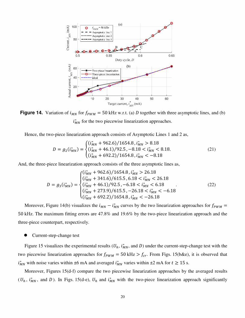
20

Figure 14. Variation of 𝑖𝑀𝑁 for 𝑓𝑃𝑊𝑀 = 50 kHz w.r.t. (a) 𝐷 together with three asymptotic lines, and (b) 𝑖𝑀𝑁∗ for the two piecewise linearization approaches.

Hence, the two-piece linearization approach consists of Asymptotic Lines 1 and 2 as,

𝐷 = 𝑔2(𝑖𝑀𝑁∗ ) = {(𝑖𝑀𝑁∗ + 962.6) 1654.8⁄ , 𝑖𝑀𝑁∗ > 8.18(𝑖𝑀𝑁∗ + 46.1) 92.5⁄ ,−8.18 < 𝑖𝑀𝑁∗ < 8.18(𝑖𝑀𝑁∗ + 692.2) 1654.8⁄ , 𝑖𝑀𝑁∗ < −8.18 . (21)

And, the three-piece linearization approach consists of the three asymptotic lines as,

𝐷 = 𝑔3(𝑖𝑀𝑁∗ ) = { (𝑖𝑀𝑁∗ + 962.6) 1654.8⁄ , 𝑖𝑀𝑁∗ > 26.18(𝑖𝑀𝑁∗ + 341.6) 615.5⁄ , 6.18 < 𝑖𝑀𝑁∗ < 26.18(𝑖𝑀𝑁∗ + 46.1) 92.5⁄ ,−6.18 < 𝑖𝑀𝑁∗ < 6.18(𝑖𝑀𝑁∗ + 273.9) 615.5⁄ ,−26.18 < 𝑖𝑀𝑁∗ < −6.18(𝑖𝑀𝑁∗ + 692.2) 1654.8⁄ , 𝑖𝑀𝑁∗ < −26.18 . (22)

Moreover, Figure 14(b) visualizes the 𝑖𝑀𝑁 − 𝑖𝑀𝑁∗ curves by the two linearization approaches for 𝑓𝑃𝑊𝑀 =50 kHz. The maximum fitting errors are 47.8% and 19.6% by the two-piece linearization approach and the

three-piece counterpart, respectively.

Current-step-change test

Figure 15 visualizes the experimental results (𝑈ℎ, 𝑖𝑀𝑁∗ , and 𝐷) under the current-step-change test with the

two piecewise linearization approaches for 𝑓𝑃𝑊𝑀 = 50 kHz > 𝑓𝑐𝑟. From Figs. 15(b&e), it is observed that 𝑖𝑀𝑁∗ with noise varies within ±6 mA and averaged 𝑖𝑀𝑁∗ varies within ±2 mA for 𝑡 ≥ 15 s.

Moreover, Figures 15(d-f) compare the two piecewise linearization approaches by the averaged results

(𝑈ℎ , 𝑖𝑀𝑁∗ , and 𝐷 ). In Figs. 15(d-e), 𝑈ℎ and 𝑖𝑀𝑁∗ with the two-piece linearization approach significantly

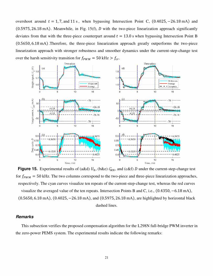
21

overshoot around 𝑡 = 1, 7, and 11 s , when bypassing Intersection Point C, (0.4025,−26.18 mA) and (0.5975, 26.18 mA). Meanwhile, in Fig. 15(f), 𝐷 with the two-piece linearization approach significantly

deviates from that with the three-piece counterpart around 𝑡 = 13.0 s when bypassing Intersection Point B (0.5650, 6.18 mA) .Therefore, the three-piece linearization approach greatly outperforms the two-piece

linearization approach with stronger robustness and smoother dynamics under the current-step-change test

over the harsh sensitivity transition for 𝑓𝑃𝑊𝑀 = 50 kHz > 𝑓𝑐𝑟.

Figure 15. Experimental results of (a&d) 𝑈ℎ, (b&e) 𝑖𝑀𝑁∗ , and (c&f) 𝐷 under the current-step-change test

for 𝑓𝑃𝑊𝑀 = 50 kHz. The two columns correspond to the two-piece and three-piece linearization approaches,

respectively. The cyan curves visualize ten repeats of the current-step-change test, whereas the red curves

visualize the averaged value of the ten repeats. Intersection Points B and C, i.e., (0.4350,−6.18 mA), (0.5650, 6.18 mA), (0.4025,−26.18 mA), and (0.5975, 26.18 mA), are highlighted by horizontal black

dashed lines.

Remarks

This subsection verifies the proposed compensation algorithm for the L298N full-bridge PWM inverter in

the zero-power PEMS system. The experimental results indicate the following remarks:

22

1) The piecewise linearization approach with more pieces can better approximate the sensitivity

transition of the nonlinear 𝑖𝑀𝑁 − 𝐷 characteristic. Besides, other fitting approaches, e.g., polynomial fitting,

can serve the same purpose as well.

2) Under the current-step-change test over the sensitivity transition, the three-piece linearization

approach successfully stabilizes the single-axis PEMS system with only a few milliampere current and

demonstrates stronger robustness and smoother dynamics than the two-piece counterpart especially for 𝑓𝑃𝑊𝑀 = 50 kHz > 𝑓𝑐𝑟.

Discussion

The present work investigates into the nonlinear mechanism of the L298N full-bridge PWM inverter,

proposes the compensation algorithm, and realizes for the zero-power PEMS system with record-breaking 𝑓𝑃𝑊𝑀 = 50 kHz . Based on the experimental observation and the theoretical analysis, we can draw the

following conclusions:

1) Nonlinear mechanism: the 2 μs turn-off delay of the IC L298N leads to the DC mode that accounts

for 𝑓𝑐𝑟 and the sensitivity transition.

2) Compensation algorithm: the piecewise linearization approach overcomes the sensitivity transition

and stabilizes the zero-power PEMS system especially for 𝑓𝑃𝑊𝑀 > 𝑓𝑐𝑟. The lower fitting error, the stronger

robustness and the smoother dynamics under the current-step-change test.

Therefore, in order to enhance the dynamic performance of the high-speed PEMS transportation, higher 𝑓𝑃𝑊𝑀 can be realized by reducing (i) the turn-off delay of the full-bridge PWM inverter and (ii) the fitting

error of the compensation algorithm.

Methods

Analog Signal Processor

Figure 16 visualizes the electric circuit of the analog signal processor. The height signal (𝑈ℎ) is generated

by the ITR8307 opto interrupter and processed by the LM324 operational amplifier for the proportional and

derivative signals (𝑈𝑝 & 𝑈𝑑), {𝑈𝑝 = (1.65 − 𝑈ℎ) 𝑅𝑃2 𝑅𝑃1⁄ + 1.65 = 1.35(1.65 − 𝑈ℎ) + 1.65𝑈𝑑 = 𝐶𝑑𝑅𝐷 𝑑(1.65 − 𝑈ℎ) 𝑑𝑡⁄ + 1.65 = −0.19 𝑑𝑈ℎ 𝑑𝑡⁄ + 1.65 (23)

where 𝑈𝑝 and 𝑈𝑑 are the two inputs to the 12-bit analog-digital converters of the STM32 controller.

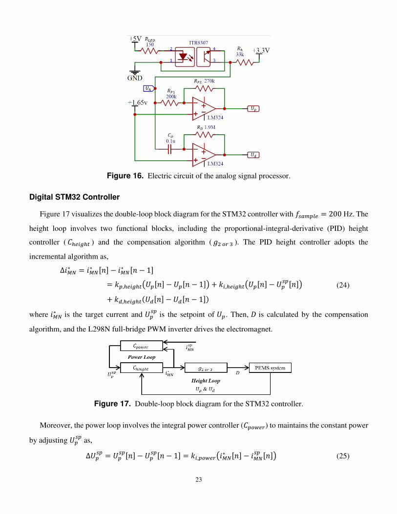
23

Figure 16. Electric circuit of the analog signal processor.

Digital STM32 Controller

Figure 17 visualizes the double-loop block diagram for the STM32 controller with 𝑓𝑠𝑎𝑚𝑝𝑙𝑒 = 200 Hz. The

height loop involves two functional blocks, including the proportional-integral-derivative (PID) height

controller ( 𝐶ℎ𝑒𝑖𝑔ℎ𝑡 ) and the compensation algorithm (𝑔2 𝑜𝑟 3 ). The PID height controller adopts the

incremental algorithm as, ∆𝑖𝑀𝑁∗ = 𝑖𝑀𝑁∗ [𝑛] − 𝑖𝑀𝑁∗ [𝑛 − 1]= 𝑘𝑝,ℎ𝑒𝑖𝑔ℎ𝑡(𝑈𝑝[𝑛] − 𝑈𝑝[𝑛 − 1]) + 𝑘𝑖,ℎ𝑒𝑖𝑔ℎ𝑡(𝑈𝑝[𝑛] − 𝑈𝑝𝑠𝑝[𝑛])+ 𝑘𝑑,ℎ𝑒𝑖𝑔ℎ𝑡(𝑈𝑑[𝑛] − 𝑈𝑑[𝑛 − 1]) (24)

where 𝑖𝑀𝑁∗ is the target current and 𝑈𝑝𝑠𝑝 is the setpoint of 𝑈𝑝. Then, 𝐷 is calculated by the compensation

algorithm, and the L298N full-bridge PWM inverter drives the electromagnet.

Figure 17. Double-loop block diagram for the STM32 controller.

Moreover, the power loop involves the integral power controller (𝐶𝑝𝑜𝑤𝑒𝑟) to maintains the constant power

by adjusting 𝑈𝑝𝑠𝑝 as, ∆𝑈𝑝𝑠𝑝 = 𝑈𝑝𝑠𝑝[𝑛] − 𝑈𝑝𝑠𝑝[𝑛 − 1] = 𝑘𝑖,𝑝𝑜𝑤𝑒𝑟(𝑖𝑀𝑁∗ [𝑛] − 𝑖𝑀𝑁𝑠𝑝 [𝑛]) (25)

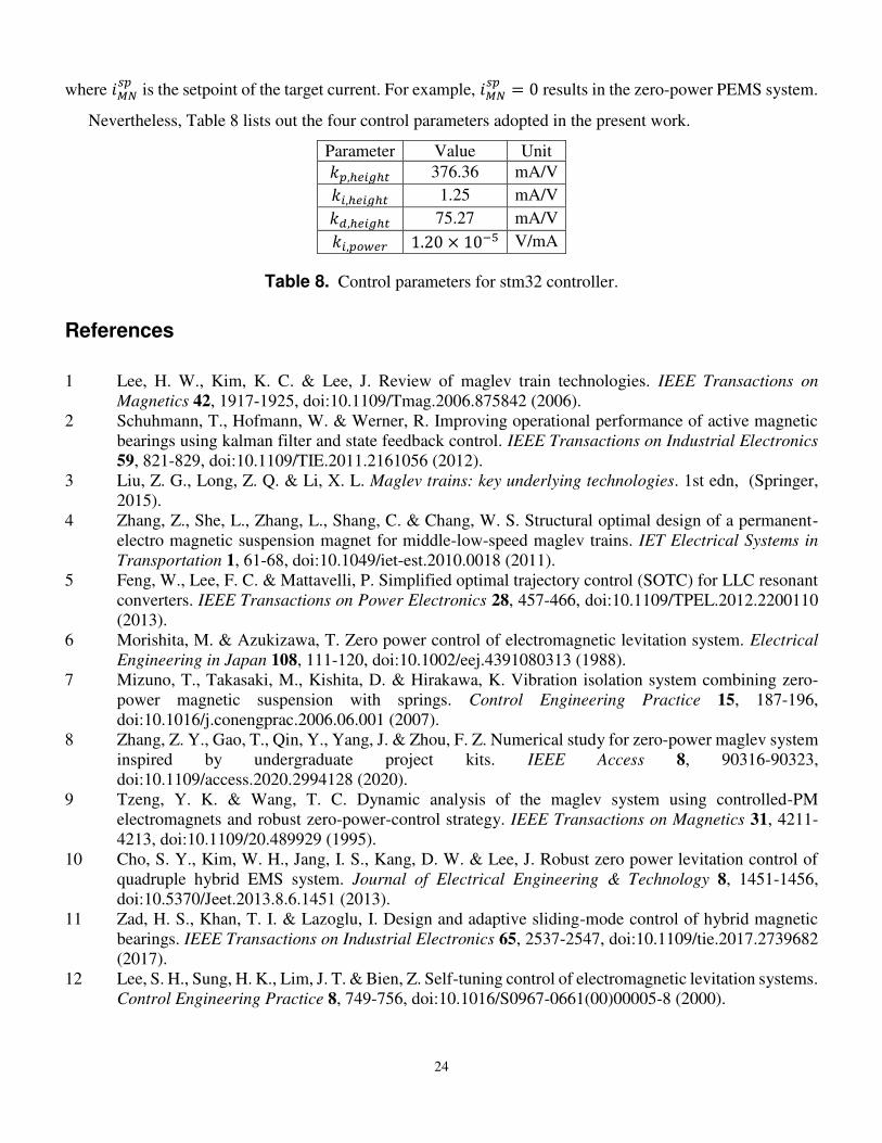
24

where 𝑖𝑀𝑁𝑠𝑝 is the setpoint of the target current. For example, 𝑖𝑀𝑁𝑠𝑝 = 0 results in the zero-power PEMS system.

Nevertheless, Table 8 lists out the four control parameters adopted in the present work.

Parameter Value Unit 𝑘𝑝,ℎ𝑒𝑖𝑔ℎ𝑡 376.36 mA/V 𝑘𝑖,ℎ𝑒𝑖𝑔ℎ𝑡 1.25 mA/V 𝑘𝑑,ℎ𝑒𝑖𝑔ℎ𝑡 75.27 mA/V 𝑘𝑖,𝑝𝑜𝑤𝑒𝑟 1.20 × 10−5 V/mA

Table 8. Control parameters for stm32 controller.

References

1 Lee, H. W., Kim, K. C. & Lee, J. Review of maglev train technologies. IEEE Transactions on

Magnetics 42, 1917-1925, doi:10.1109/Tmag.2006.875842 (2006).

2 Schuhmann, T., Hofmann, W. & Werner, R. Improving operational performance of active magnetic

bearings using kalman filter and state feedback control. IEEE Transactions on Industrial Electronics

59, 821-829, doi:10.1109/TIE.2011.2161056 (2012).

3 Liu, Z. G., Long, Z. Q. & Li, X. L. Maglev trains: key underlying technologies. 1st edn, (Springer,

2015).

4 Zhang, Z., She, L., Zhang, L., Shang, C. & Chang, W. S. Structural optimal design of a permanent-

electro magnetic suspension magnet for middle-low-speed maglev trains. IET Electrical Systems in

Transportation 1, 61-68, doi:10.1049/iet-est.2010.0018 (2011).

5 Feng, W., Lee, F. C. & Mattavelli, P. Simplified optimal trajectory control (SOTC) for LLC resonant

converters. IEEE Transactions on Power Electronics 28, 457-466, doi:10.1109/TPEL.2012.2200110

(2013).

6 Morishita, M. & Azukizawa, T. Zero power control of electromagnetic levitation system. Electrical

Engineering in Japan 108, 111-120, doi:10.1002/eej.4391080313 (1988).

7 Mizuno, T., Takasaki, M., Kishita, D. & Hirakawa, K. Vibration isolation system combining zero-

power magnetic suspension with springs. Control Engineering Practice 15, 187-196,

doi:10.1016/j.conengprac.2006.06.001 (2007).

8 Zhang, Z. Y., Gao, T., Qin, Y., Yang, J. & Zhou, F. Z. Numerical study for zero-power maglev system

inspired by undergraduate project kits. IEEE Access 8, 90316-90323,

doi:10.1109/access.2020.2994128 (2020).

9 Tzeng, Y. K. & Wang, T. C. Dynamic analysis of the maglev system using controlled-PM

electromagnets and robust zero-power-control strategy. IEEE Transactions on Magnetics 31, 4211-

4213, doi:10.1109/20.489929 (1995).

10 Cho, S. Y., Kim, W. H., Jang, I. S., Kang, D. W. & Lee, J. Robust zero power levitation control of

quadruple hybrid EMS system. Journal of Electrical Engineering & Technology 8, 1451-1456,

doi:10.5370/Jeet.2013.8.6.1451 (2013).

11 Zad, H. S., Khan, T. I. & Lazoglu, I. Design and adaptive sliding-mode control of hybrid magnetic

bearings. IEEE Transactions on Industrial Electronics 65, 2537-2547, doi:10.1109/tie.2017.2739682

(2017).

12 Lee, S. H., Sung, H. K., Lim, J. T. & Bien, Z. Self-tuning control of electromagnetic levitation systems.

Control Engineering Practice 8, 749-756, doi:10.1016/S0967-0661(00)00005-8 (2000).

25

13 Wai, R. J., Lee, J. D. & Chuang, K. L. Real-time PID control strategy for maglev transportation system

via particle swarm optimization. IEEE Transactions on Industrial Electronics 58, 629-646,

doi:10.1109/Tie.2010.2046004 (2011).

14 Banerjee, S., Sarkar, M. K., Biswas, P. K., Bhaduri, R. & Sarkar, P. A review note on different

components of simple electromagnetic levitation systems. IETE Technical Review 28, 256-264,

doi:10.4103/0256-4602.81241 (2011).

15 WANG, Z. Q., LONG, Z. Q. & LI, X. L. Track irregularity disturbance rejection for maglev train

based on online optimization of PnP control architecture. IEEE Access 7, 12610 - 12619,

doi:10.1109/ACCESS.2019.2891964 (2019).

16 Carmichael, A. T., Hinchliffe, S., Murgatroyd, P. N. & Williams, I. D. Magnetic suspension systems

with digital controllers. Review of Scientific Instruments 57, 1611-1615, doi:10.1063/1.1138539

(1986).

17 Zhang, Y., Xian, B. & Ma, S. Continuous robust tracking control for magnetic levitation system with

unidirectional input constraint. IEEE Transactions on Industrial Electronics 62, 5971-5980,

doi:10.1109/TIE.2015.2434791 (2015).

18 Mittal, S. & Menq, C. H. Precision motion control of a magnetic suspension actuator using a robust

nonlinear compensation scheme. IEEE/ASME Transactions on Mechatronics 2, 268-280,

doi:10.1109/3516.653051 (1997).

19 Zhang, C., Lu, Y. H., Liu, G. C. & Ye, Z. B. Research on one-dimensional motion control system and

method of a magnetic levitation ball. Review of Scientific Instruments 90, 1-9, doi:10.1063/1.5119767

(2019).

Acknowledgements

This work was supported in part by the high-level talents research start-up project of Jiangxi

University of Science and Technology under Grant 205200100476.

Author contributions statement

This is a single-author paper.

Additional information

Correspondence and requests for materials should be addressed to Z.Z.

Competing interests statement

The author(s) declare no competing interests.

Legends

26

Figure 1. Close-loop architecture of the single-axis PEMS system.

Figure 2. Hardware of the single-axis PEMS system, (a) stereoscopic view and (b) cross-sectional view for

the electromagnet and the permanent magnet, (c) electronic devices, and (d) experiment rig.

Figure 3. Nonlinear characteristic of the ITR8307 distance sensor.

Figure 4. Electric circuit of L298N full-bridge PWM inverter.

Figure 5. Variations of (a) 𝑖𝑀𝑁 and (b) 𝑆 w.r.t. 𝐷 for 𝑓𝑃𝑊𝑀 = 0.1,1,10,100 kHz.

Figure 6. Whole-period variations of (a) 𝐼𝑛1 and 𝐼𝑛2, (b) 𝑈𝑀 and 𝑈𝑁, and (c) 𝑢𝑀𝑁 for 𝑓𝑃𝑊𝑀 = 100 kHz

and 𝐷 = 0.5 w.r.t. 𝑡. The 2 μs turn-off delay due to the IC L298N can be clearly observed for both 𝑈𝑀 and 𝑈𝑁 in (b). Three modes are highlighted in (c) according to 𝑢𝑀𝑁.

Figure 7. Whole-period variation of 𝑢𝑀𝑁 for 𝑓𝑃𝑊𝑀 = 100 Hz and 𝐷 = 0.5 w.r.t. 𝑡. The red dashed lines

(𝑢𝑀𝑁 = ±12 V) indicate the boundaries between the FC and BC modes.

Figure 8. Initial-3-μs variations of 𝑢𝑀𝑁 w.r.t. 𝑡 for 𝑓𝑃𝑊𝑀 = 5, 10, 20, 50, and 100 kHz and 𝐷 = 0.5.

Figure 9. Initial-20-ms variations of 𝑢𝑀𝑁 w.r.t. 𝑡 for 𝑓𝑃𝑊𝑀 = 2, 10, 20, 50, 100, and 200 Hz and 𝐷 = 0.5.

Note that the 2 Hz and 10 Hz curves almost overlap with each other. The black dash-dot line (𝑢𝑀𝑁 = +10 V)

indicates the saturation of the FC mode.

Figure 10. Contour of 𝑢𝑀𝑁 w.r.t. log10(𝑓𝑃𝑊𝑀) and 𝑡 𝑇⁄ for 𝐷 = 0.5. The green dotted curves (𝑢𝑀𝑁 =±9.5 V) indicate the boundaries between the DC mode and the two charging modes.

Figure 11. (a-c) Phase diagrams of 𝑢𝑀𝑁 w.r.t. 𝐷 and 𝑡 𝑇⁄ , and (d-f) variations of 𝑆 w.r.t. 𝐷 for 𝑓𝑃𝑊𝑀 =1, 10, and 100 kHz. The cyan dotted lines indicate the termination points of the FC regimes, whereas the

purple dotted lines indicate the transition points with 𝑆 = 1000 mA . The dashed curve in (d&f) is the

benchmark curve with 𝑓𝑃𝑊𝑀 = 10 kHz.

Figure 12. Variation of 𝑖𝑀𝑁 for 𝑓𝑃𝑊𝑀 = 10 kHz w.r.t. (a) 𝐷 together with three asymptotic lines, and (b) 𝑖𝑀𝑁∗ for the two piecewise linearization approaches.

Figure 13. Experimental results of (a&d) 𝑈ℎ, (b&e) 𝑖𝑀𝑁∗ , and (c&f) 𝐷 under the current-step-change test for 𝑓𝑃𝑊𝑀 = 10 kHz. The two columns correspond to the two-piece and three-piece linearization approaches,

27

respectively. The cyan curves visualize ten repeats of the current-step-change test, whereas the red curves

visualize the averaged value of the ten repeats. Intersection Points B and C, i.e., (0.4374,−12.48 mA), (0.5626, 12.48 mA), (0.4026, −49.77 mA), and (0.5974, 49.77 mA), are highlighted by horizontal black

dashed lines.

Figure 14. Variation of 𝑖𝑀𝑁 for 𝑓𝑃𝑊𝑀 = 50 kHz w.r.t. (a) 𝐷 together with three asymptotic lines, and (b)

Figure 15. Experimental results of (a&d) 𝑈ℎ, (b&e) 𝑖𝑀𝑁∗ , and (c&f) 𝐷 under the current-step-change test for 𝑓𝑃𝑊𝑀 = 50 kHz. The two columns correspond to the two-piece and three-piece linearization approaches,

respectively. The cyan curves visualize ten repeats of the current-step-change test, whereas the red curves

visualize the averaged value of the ten repeats. Intersection Points B and C, i.e., (0.4350,−6.18 mA) , (0.5650, 6.18 mA), (0.4025,−26.18 mA), and (0.5975, 26.18 mA), are highlighted by horizontal black

dashed lines.

Figure 16. Electric circuit of the analog signal processor.

Figure 17. Double-loop block diagram for the STM32 controller.

Table 1. Physical properties of the single-axis PEMS system.

Table 2. Three modes of full-bridge PWM inverter with electromagnet.

Table 3. Four quadrants of full-bridge PWM inverter with electromagnet.

Table 4. Relative portions of three modes for various 𝑓𝑃𝑊𝑀 and 𝐷 = 0.5.

Table 5. Estimated relative portions of three modes and associated fitting errors for various 𝑓𝑃𝑊𝑀 and 𝐷 =0.5.

Table 6. Evolution of three modes w.r.t. 𝐷 ≥ 0.5 for 𝑓𝑃𝑊𝑀 < 𝑓𝑐𝑟.

Table 7. Evolution of three modes w.r.t. 𝐷 ≥ 0.5 for 𝑓𝑃𝑊𝑀 > 𝑓𝑐𝑟.

Table 8. Control parameters for stm32 controller.

Figures

Figure 1

Close-loop architecture of the single-axis PEMS system.

Figure 2

Hardware of the single-axis PEMS system, (a) stereoscopic view and (b) cross-sectional view for theelectromagnet and the permanent magnet, (c) electronic devices, and (d) experiment rig.

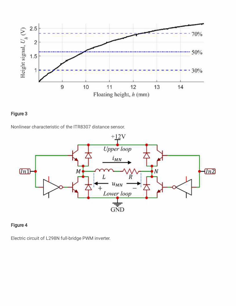
Figure 3

Nonlinear characteristic of the ITR8307 distance sensor.

Figure 4

Electric circuit of L298N full-bridge PWM inverter.

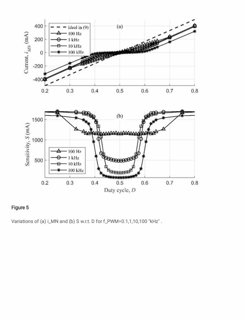
Figure 5

Variations of (a) i_MN and (b) S w.r.t. D for f_PWM=0.1,1,10,100 "kHz" .

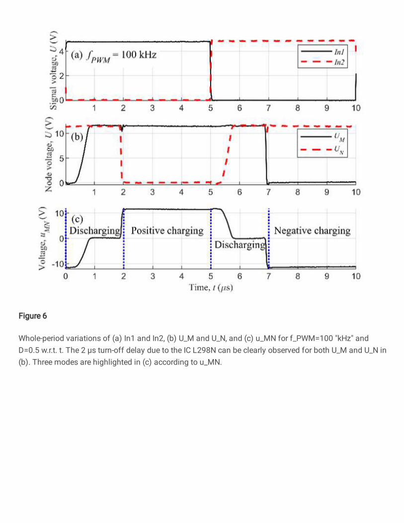
Figure 6

Whole-period variations of (a) In1 and In2, (b) U_M and U_N, and (c) u_MN for f_PWM=100 "kHz" andD=0.5 w.r.t. t. The 2 μs turn-off delay due to the IC L298N can be clearly observed for both U_M and U_N in(b). Three modes are highlighted in (c) according to u_MN.

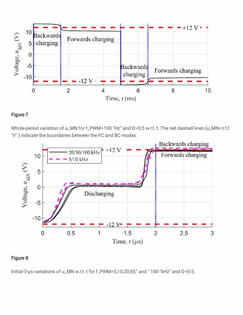
Figure 7

Whole-period variation of u_MN for f_PWM=100 "Hz" and D=0.5 w.r.t. t. The red dashed lines (u_MN=±12"V" ) indicate the boundaries between the FC and BC modes.

Figure 8

Initial-3-μs variations of u_MN w.r.t. t for f_PWM=5,10,20,50," and " 100 "kHz" and D=0.5.

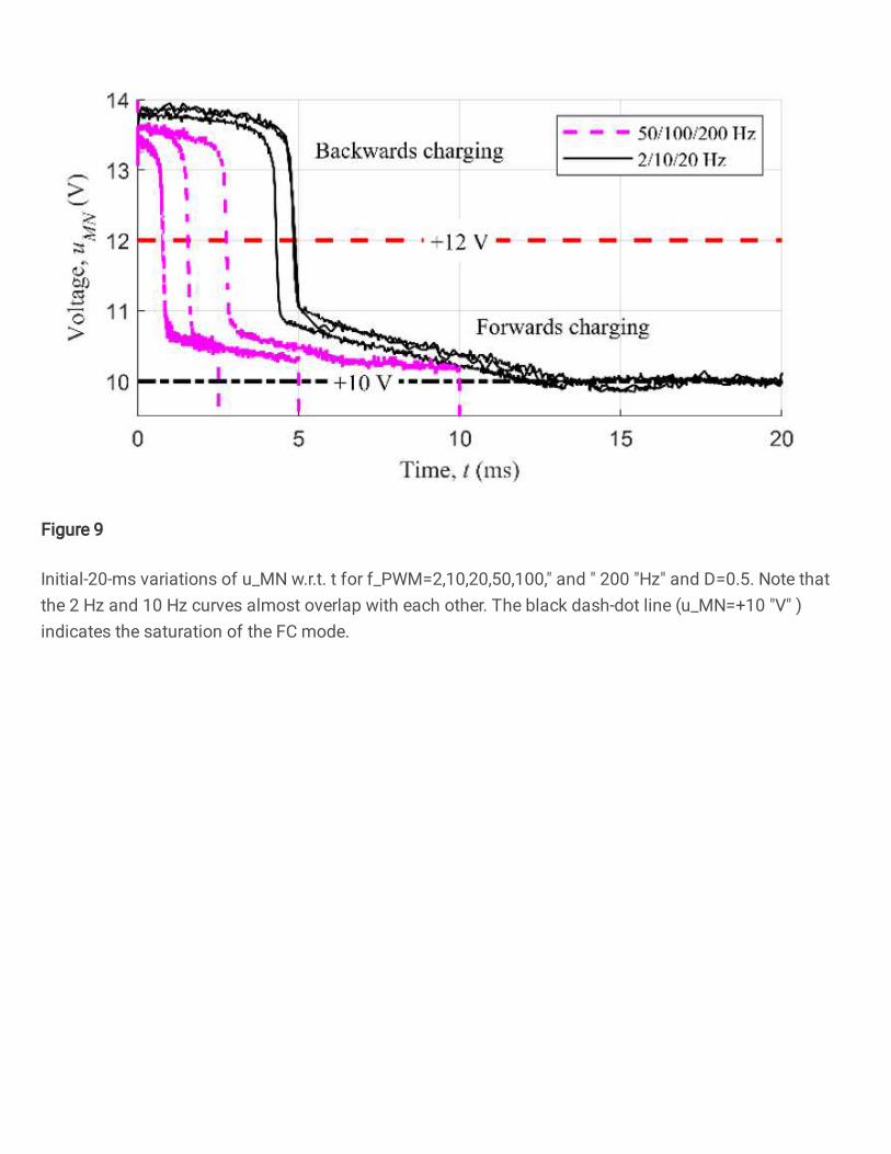
Figure 9

Initial-20-ms variations of u_MN w.r.t. t for f_PWM=2,10,20,50,100," and " 200 "Hz" and D=0.5. Note thatthe 2 Hz and 10 Hz curves almost overlap with each other. The black dash-dot line (u_MN=+10 "V" )indicates the saturation of the FC mode.

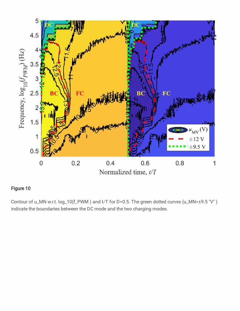
Figure 10

Contour of u_MN w.r.t. log_10 (f_PWM ) and t⁄T for D=0.5. The green dotted curves (u_MN=±9.5 "V" )indicate the boundaries between the DC mode and the two charging modes.

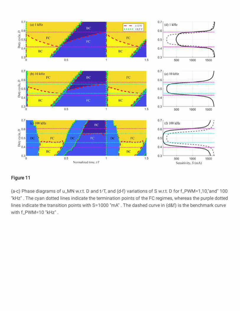
Figure 11

(a-c) Phase diagrams of u_MN w.r.t. D and t⁄T, and (d-f) variations of S w.r.t. D for f_PWM=1,10,"and" 100"kHz" . The cyan dotted lines indicate the termination points of the FC regimes, whereas the purple dottedlines indicate the transition points with S=1000 "mA" . The dashed curve in (d&f) is the benchmark curvewith f_PWM=10 "kHz" .

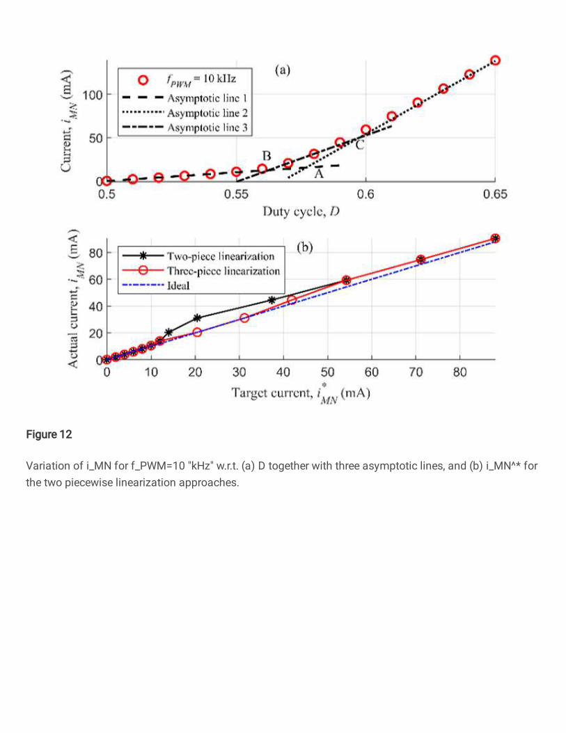
Figure 12

Variation of i_MN for f_PWM=10 "kHz" w.r.t. (a) D together with three asymptotic lines, and (b) i_MN^* forthe two piecewise linearization approaches.

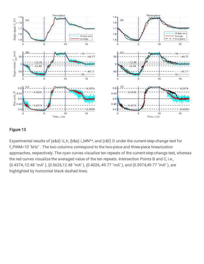
Figure 13

Experimental results of (a&d) U_h, (b&e) i_MN^*, and (c&f) D under the current-step-change test forf_PWM=10 "kHz" . The two columns correspond to the two-piece and three-piece linearizationapproaches, respectively. The cyan curves visualize ten repeats of the current-step-change test, whereasthe red curves visualize the averaged value of the ten repeats. Intersection Points B and C, i.e.,(0.4374,-12.48 "mA" ), (0.5626,12.48 "mA" ), (0.4026,-49.77 "mA" ), and (0.5974,49.77 "mA" ), arehighlighted by horizontal black dashed lines.

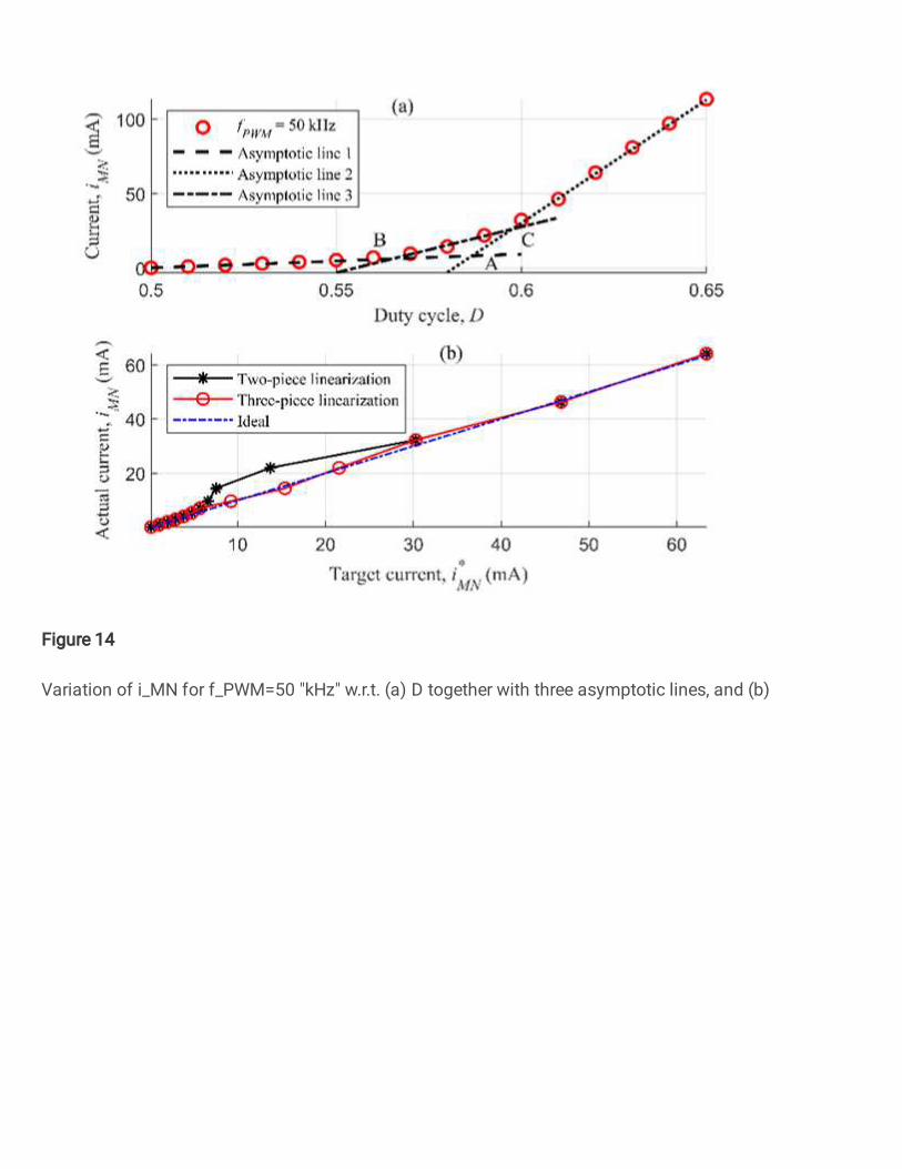
Figure 14

Variation of i_MN for f_PWM=50 "kHz" w.r.t. (a) D together with three asymptotic lines, and (b)

Figure 15

Experimental results of (a&d) U_h, (b&e) i_MN^*, and (c&f) D under the current-step-change test forf_PWM=50 "kHz" . The two columns correspond to the two-piece and three-piece linearizationapproaches, respectively. The cyan curves visualize ten repeats of the current-step-change test, whereasthe red curves visualize the averaged value of the ten repeats. Intersection Points B and C, i.e.,(0.4350,-6.18 "mA" ), (0.5650,6.18 "mA" ), (0.4025,-26.18 "mA" ), and (0.5975,26.18 "mA" ), are highlightedby horizontal black dashed lines.

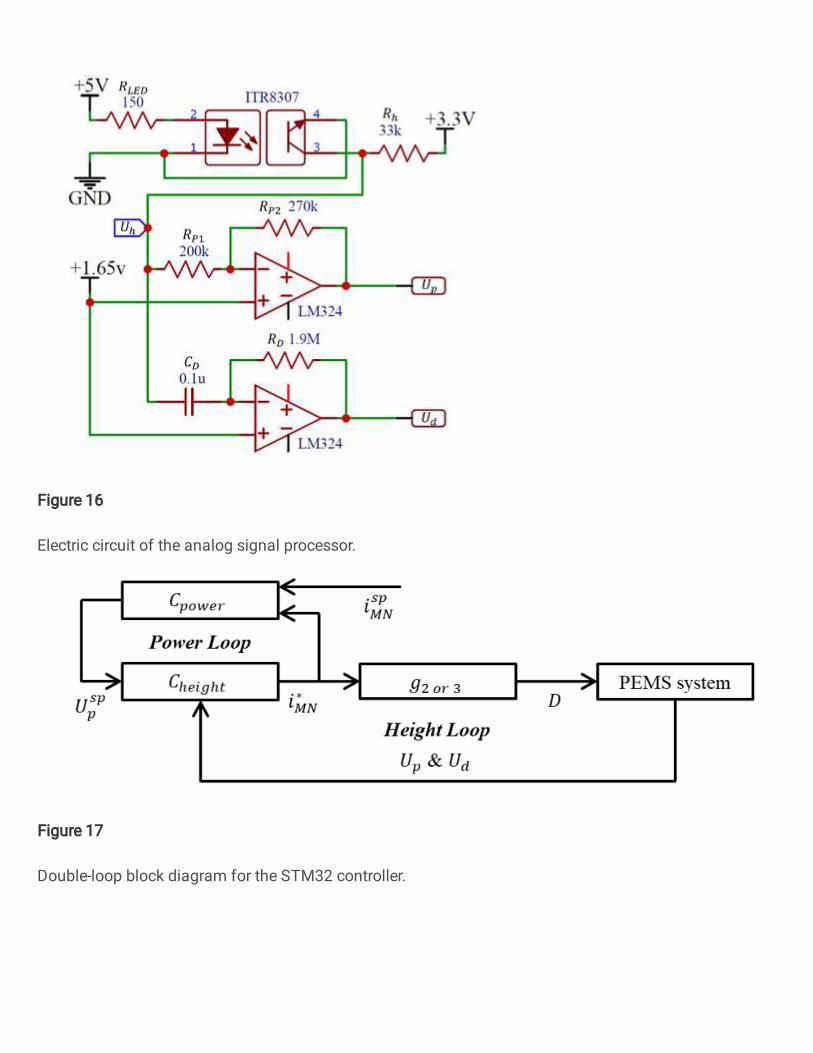
Figure 16

Electric circuit of the analog signal processor.

Figure 17

Double-loop block diagram for the STM32 controller.