Zero-Knowledge Against Quantum Attacks

John Watrous

Institute for Quantum Computing and School of Computer Science

University of Waterloo, Waterloo, Ontario, Canada

April 24, 2008(with minor corrections on April 14, 2009)

Abstract

It is proved that several interactive proof systems are zero-knowledge against general quan-tum attacks. This includes the Goldreich–Micali–Wigderson classical zero-knowledge proto-cols for Graph Isomorphism and Graph 3-Coloring (assuming the existence of quantum com-putationally concealing commitment schemes in the second case). Also included is a quantuminteractive proof system for a complete problem for the complexity class of problems hav-ing honest verifier quantum statistical zero-knowledge proofs, which therefore establishes thathonest verifier and general quantum statistical zero-knowledge are equal: QSZK = QSZKHV.Previously no non-trivial interactive proof systems were known to be zero-knowledge againstquantum attacks, except in restricted settings such as the honest-verifier and common refer-ence string models. This paper therefore establishes for the first time that true zero-knowledgeis indeed possible in the presence of quantum information and computation.

1 Introduction

The security of classical cryptographic systems against quantum computer attacks has the poten-tial to become an issue of critical importance in cryptography in years to come. It is well-known,for instance, that Shor’s algorithm [Sho97] allows for efficient quantum cryptanalysis of manypublic-key cryptosystems such as RSA [RSA78]. In the event that large-scale quantum comput-ing becomes technologically feasible, these cryptosystems will therefore be rendered completelyinsecure. While quantum cryptography offers a secure alternative in the case of key-exchange[BB84, May01, SP00], it is not reasonable to expect that quantum cryptographic systems will be-come widely used in the near future—even the relatively low technological requirements of quan-tum key exchange are presently well beyond the means of most computer users. A more practicalsolution is to design classical cryptosystems that are secure against quantum computer attacks.

This paper investigates the security of zero-knowledge interactive proof systems against quan-tum computer attacks. Although both quantum and classical interactive proof systems are con-sidered, the main focus of this paper is on the security of classical zero-knowledge proof systemsagainst quantum attacks. This is the case of greatest practical importance, for the reasons sug-gested above. Independent of present-day progress toward large-scale quantum computing, thisstudy is motivated by an obvious goal in cryptography: to prove security of cryptosystems againstas wide a range of malicious attacks as possible, while at the same time minimizing the resourcerequirements of honest users.

1

The notion of zero-knowledge was introduced by Goldwasser, Micali and Rackoff [GMR89].Informally speaking, an interactive proof systemhas the property of being zero-knowledge if arbi-trary verifiers that interact with the honest prover of the system learn nothing from the interactionbeyond the validity of the statement being proved. At first consideration this notion may seem tobe paradoxical, but indeed several interesting computational problems that are not known to bepolynomial-time computable admit zero-knowledge interactive proof systems in the classical set-ting. Examples include the Graph Isomorphism [GMW91] and Quadratic Residuosity [GMR89]problems, various lattice problems [GG00], and the Statistical Difference [SV03] and Entropy Dif-ference [GV99] problems, which concern outputs of Boolean circuits with random inputs. Thefact that the last three examples have interactive proof systems that are zero-knowledge relieson a fundamental result of Goldreich, Sahai and Vadhan [GSV98] equating zero-knowledge withhonest verifier zero-knowledge in some settings. Under certain intractability assumptions, everylanguage in NP has a zero-knowledge interactive proof system [GMW91]. A related notion is thatof interactive arguments, which differ from interactive proof systems in that computational restric-tions are placed on the prover as well as the verifier [BCC88]. In the interactive argument setting,zero-knowledge protocols exist that have somewhat different characteristics than protocols in theinteractive proof system setting.

There are several variants of zero-knowledge that differ in the way that the notion of “learningnothing” is formalized. In each variant, it is viewed that a particular verifier learns nothing ifthere exists a polynomial-time simulator whose output is indistinguishable from the output of theverifier when the honest prover and verifier interact on any positive instance of the problem.The different variants concern the strength of this indistinguishability. In particular, perfect andstatistical zero-knowledge refer to the situation where the simulator’s output and the verifier’soutput are indistinguishable in an information-theoretic sense and computational zero-knowledgerefers to the weaker restriction that the simulator’s output and the verifier’s output cannot bedistinguished by any computationally efficient procedure.

The security of zero-knowledge proof systems against quantum verifiers has been a topic ofstudy for several years [Gra97, Wat02, Kob03, DFS04]. Progress has been slow, however, for asimple reason—while it is straightforward to formulate natural quantum analogues of the classi-cal definitions of zero-knowledge, no interactive proof systems or interactive arguments could beshown to satisfy these definitions prior to this paper. This has left open several possibilities, in-cluding the possibility that any “correct” definition of quantum zero-knowledge would necessar-ily be qualitatively different from the usual classical definitions, as well as the possibility that zero-knowledge is simply impossible in a quantumworld. The fundamental difficulty that one encoun-ters when trying to apply these quantum definitions was first discovered by van de Graaf [Gra97],and will be discussed shortly.

The main task involved in proving that a given interactive proof system is zero-knowledgeis the construction of a simulator for every possible deviant polynomial-time verifier. The mosttypical method for doing this involves the simulator treating a given verifier as a black box: thesimulator randomly generates transcripts, or parts of transcripts, of possible interactions betweena prover and verifier, and feeds parts of these transcripts to the given verifier. If the verifier pro-duces a message that is not consistent with the other parts of the transcript that were generated,the simulator rewinds, or backs up and tries again to randomly generate parts of the transcript. Bystoring intermediate results, and repeating different parts of this process until the given verifier’soutput is consistent with a randomly generated transcript, the simulation is eventually successful.

In the quantum setting, the rewinding technique faces two basic obstacles that are uniqueto quantum information. The first is the no-cloning theorem [WZ82], which states that unknownquantum states cannot be copied, and the second is the principle of information gain versus state dis-

2

turbance (see Fuchs and Peres [FP96], for instance). Quantum verifiers may store and manipulatequantum information, andmay even begin a given protocolwith auxiliary quantum information—perhaps resulting from a previous iteration of the protocol being considered. A simulator cannotmake copies of the verifier’s quantum state at any given time, and must therefore treat the quan-tum information stored by the verifier very carefully. This makes rewinding problematic, becauseif the simulation of given verifier is inconsistent with an actual interaction at some point, it is notobvious how to rewind the process and try again: measurements made by the simulator, such asones providing information about the success of the simulation, will generally cause a disturbancein the quantum information it stores.

Other methods of constructing simulators for quantum verifiers have also been considered, inan attempt to circumvent the problematic rewinding issue. For example, Damgard, Fehr, andSalvail [DFS04] proved several interesting results concerning quantum zero-knowledge proto-cols in the common reference string model, wherein it is assumed that an honest third party sam-ples a string from some specified distribution and provides both the prover and verifier withthis string at the start of the interaction. Their results, based on what they call the no quantumrewinding paradigm, are mostly concerned with interactive arguments and rely on certain quantumcomplexity-theoretic intractability assumptions. Anotherweaker notion of zero-knowledge is hon-est verifier zero-knowledge, which only requires that a simulator outputs the honest verifier’s viewof an interaction with the honest prover P. A quantum variant of honest verifier statistical zero-knowledge was considered in [Wat02], wherein it was proved that the resulting complexity classQSZKHV shares many of the basic properties of its classical counterpart [SV03]. A non-interactivevariant of this notion was studied by Kobayashi [Kob03]. The problematic issue regarding simu-lator constructions does not occur in honest verifier settings.

The present paper resolves, at least to a significant extent, the main difficulties previously as-sociated with quantum analogues of zero-knowledge. This is done by establishing that the mostnatural quantum analogues of the classical definitions of zero-knowledge indeed can be appliedto a large class of interactive proof systems. This includes some well-known classical interactiveproof systems as well as quantum interactive proof systems for several problems, in particularthe class of all problems admitting quantum interactive proof systems that are statistical zero-knowledge against honest verifiers. It is therefore proved unconditionally that zero-knowledgeindeed is possible in the presence of quantum information and computation, and moreover thatthe notion of quantum zero-knowledge is correctly captured by the most natural and direct quan-tum analogues of the classical definitions.

The main technique that is introduced in this paper is algorithmic in nature: it is shown how toconstruct efficient quantum simulators for arbitrary quantum polynomial-time verifiers for sev-eral interactive proof systems. These simulators rely on a general Quantum Rewinding Lemmathat establishes simple conditions under which the success probabilities of certain processes withquantum inputs and outputs can be amplified.

The remainder of this paper is organized as follows. Section 2 gives a summary of key conceptsneeded throughout the paper, including interactive proof systems, zero-knowledge, and variousquantum information-theoretic notions; Section 3 states the definitions of quantum statistical andcomputational zero-knowledge that are studied in the sections that follow; and Section 4 containsa statement and proof of the Quantum Rewinding Lemma, which encapsulates the main technicaltool that is used to prove the security of various zero-knowledge interactive proof systems againstquantum attacks. The remaining sections are Section 5, which discusses quantum statistical zero-knowledge protocols, and Section 6, which discusses quantum computational zero-knowledgeprotocols. The paper concludes with Section 7.

3

2 Preliminaries

This section is intended to summarize some of the notation, conventions, and known facts con-cerning interactive proof systems, zero-knowledge, and quantum information and computationthat are used throughout the paper. The reader is assumed to be familiar with basic computationalcomplexity as well as quantum information and computation. These topics are independentlycovered in several books [AB06, Pap94, NC00, KSV02], to which the reader is referred for fur-ther details. Most of the complexity-theoretic facts proved in this paper are expressed in terms ofpromise problems, which are discussed in Refs. [ESY84, Gol05]. Further information on interactiveproof systems and zero-knowledge can be found in [Gol01], and information on quantum variantsof interactive proof systems can be found in [KW00].

For the rest of the paper let us fix the alphabet Σ = {0, 1}, and only consider strings, promiseproblems, and complexity classes over this alphabet. When we say that a function g having theform g : {0, 1, 2, . . .} → {1, 2, 3, . . .} is a polynomially bounded function, we mean that there existsa deterministic Turing machine Mg such that (i) on input 1n, Mg outputs 1g(n), for every non-negative integer n, and (ii) the running time of Mg is bounded by some polynomial p. A functionhaving the form f : {0, 1, 2, . . .} → (0,∞) is said to be negligible if, for every polynomially boundedfunction g, it holds that f (n) < 1/g(n) for all but finitely many values of n.

2.1 Interactive proof systems

Interactive proof systems will be specified by pairs (V, P) representing an honest verifier andhonest prover. The soundness property of such an interactive proof system concerns interac-tions between pairs (V, P′) and the zero-knowledge property concerns interactions between pairs(V ′, P), where P′ and V ′ deviate arbitrarily from P and V, respectively. It may be the case thata given prover/verifier pair is such that both are classical, both are quantum, or one is classicaland the other is quantum. When either or both of the parties is classical, all communication be-tween them is (naturally) assumed to be classical—only two quantum parties are permitted totransmit quantum information to one another. It will always be assumed that verifiers are rep-resented by polynomial-time (quantum or classical) computations. Depending on the setting ofinterest, the honest prover Pmay either be computationally unrestricted or may be represented bya polynomial-time (quantum or classical) computation augmented by specific information aboutthe input string, such as a witness for an NP problem. Deviant provers will be assumed to becomputationally unrestricted. (The results of this paper are applicable to interactive argumentsbut none are specific to them, and so for simplicity they are not considered further.)

For a given promise problem A = (Ayes, Ano), we say that a pair (V, P) is an interactive proofsystem for A having completeness error ε and soundness error δ if (i) for every input x ∈ Ayes,the interaction between P and V causes V to accept with probability at least 1 − ε, and (ii) forevery input x ∈ Ano and every prover P′, the interaction between P′ and V causes V to acceptwith probability at most δ. It may be the case that ε and δ are constant or are functions of thelength of the input string x. When they are functions, it is assumed that they can be computeddeterministically in polynomial time. It is generally desired that ε and δ are exponentially small;but because sequential repetition followed by majority vote, or unanimous vote in case ε = 0,reduces these errors exponentially quickly, it is usually sufficient that 1− ε − δ is lower-boundedby the reciprocal of a polynomial. A similar statement holds for parallel repetition, but the zero-knowledge property to be discussed shortly will generally be lost in this case.

4

2.2 Classical zero-knowledge

There are different notions of what it means for an interactive proof system (V, P) for a promiseproblem A to be zero-knowledge. At this point we will just discuss the completely classical case,meaning that only classical verifiers are considered.

An arbitrary verifier V ′ takes two strings as input: a string x representing the common inputto both the verifier and prover, as well as a string w called an auxiliary input, which is not knownto the prover and which may influence the verifier’s behavior during the interaction. Based onthe interaction with P, the verifier V ′ produces a string as output. For a given input string x, letn = q(|x|) denote the length of the auxiliary input string and let m = r(|x|) denote the length ofthe output string, for polynomially bounded functions q and r. Because there may be randomnessused by either or both of P and V ′, the verifier’s output will in general be random. The (string-valued) random variable representing the verifier’s output will be written (V ′(w), P)(x). For thehonest verifier V, we may view that n = 0 and m = 1 for all x ∈ Σ∗, because there is no auxiliaryinput and the output is a single bit that indicates whether the verifier accepts or rejects. By a(classical) simulator for a verifier V ′, we mean a polynomial-time randomized algorithm SV′ thattakes the stringsw and x as input and produces some output string of lengthm. Such a simulator’soutput is a random variable denoted SV′(w, x). Note that the simulator does not interact with theprover.

Now, for a given promise problem A, we say that an interactive proof system (V, P) for Ais zero-knowledge if, for every verifier V ′, there exists a simulator SV′ such that (V ′(w), P)(x) andSV′(w, x) are indistinguishable for every choice of strings x ∈ Ayes and w ∈ Σn. The specificformalization of the word “indistinguishable” gives rise to different variants of zero-knowledge.Statistical zero-knowledge refers to the situation in which (V(w), P)(x) and SV′(w, x) have negli-gible statistical difference, and computational zero-knowledge refers to the situation in which noBoolean circuit with size polynomial in |x| can distinguish (V ′(w), P)(x) and SV′(w, x) with anon-negligible advantage over randomly guessing. Perfect zero-knowledge is slightly strongerthan statistical zero-knowledge in that it essentially requires a zero-error simulation: the simula-tor may report failure with some small probability, but conditioned on the simulator not reportingfailure the output SV′(w, x) of the simulator is distributed identically to (V ′(w), P)(x). We willonly consider statistical and computational zero-knowledge once we move to the quantum case.

Two points concerning the definitions just discussed should be mentioned. The first point con-cerns the auxiliary input, which actually was not included in the definitions given in the very firstpapers on zero-knowledge (but which already appeared in the 1989 journal version of [GMR89]).The inclusion of an auxiliary input in the definition is critical: it is necessary for the closure of zero-knowledge interactive proof systems under sequential composition [GK96]. Informally speaking,the inclusion of auxiliary inputs in the definition captures the notion that a given zero-knowledgeinteractive proof system cannot be used to increase knowledge, as opposed to prohibiting one fromgaining knowledge starting from none. The second point concerns the order of quantification be-tweenV ′ and SV′ . Specifically, the definition states that a zero-knowledge interactive proof systemis one such that for all V ′ there exists a simulator SV′ that satisfies the requisite properties. Thereis an argument to be made for reversing these quantifiers by requiring that for a given interactiveproof system (V, P) there should exist a single simulator S that interfaces in some uniform waywith any given V ′ to produce an output that is indistinguishable from that verifier’s output. Typi-cal simulator constructions, as well as the ones that will be discussed in this paper in the quantumsetting, do indeed satisfy this stronger requirement.

5

2.3 Quantum information and computation

By a quantum register, we simply mean a collection of qubits that we wish to view as a single unitand to which we give some name. Names of registers will always be uppercase letters in sans seriffont, such as X, Y, and Z. The finite dimensional Hilbert spaces associated with registers will bedenoted by capital script letters such as X , Y , andZ , and it will generally be convenient to use thesame letter in the two different fonts to denote a quantum register and its corresponding space.Dirac notation is used to express vectors in Hilbert spaces and linear mappings between them ina standard way. The norm of a vector |ψ〉 is written ‖|ψ〉‖, and the all-zero standard basis vectorin a given space X is denoted |0X 〉.

For given spaces X and Y , the following notation is used to represent various sets of linearmappings from X to Y . We let L (X ,Y) denote the set of all linear mappings (or operators) from Xto Y , and write L (X ) as shorthand for L (X ,X ). The set Pos (X ) consists of all positive semidefi-nite operators acting on X , and D (X ) denotes the set of unit trace, positive semidefinite operators(i.e., density operators) acting onX . Finally, we denote the set of unitary operators onX by U (X ).The identity element of L (X ) is denoted 1X .

A linear super-operator Φ : L (X ) → L (Y) is said to be admissible if it is completely positiveand preserves trace. Admissible super-operators represent mappings from density operators todensity operators that are physically realizable (in an idealized sense).

2.3.1 Measures of similarity and distance

The concept of quantum zero-knowledge requires formal notions of distance between quantumstates and between admissible super-operators. The specific notions we will make use of aresummarized in this section.

The operator norm of an operator X ∈ L (X ,Y) is defined as

‖X‖ def= max{‖X |ψ〉‖ : |ψ〉 ∈ X , ‖|ψ〉‖ = 1},

and the trace norm is defined as‖X‖1

def= Tr

√X∗X.

The significance of the trace norm in quantum information is that it relates very closely to theoptimal probability with which two density operators can be distinguished by means of somemeasurement. In essence, the trace norm functions in a similar way to the 1-norm for differencesbetween probability distributions.

For positive semidefinite operators X,Y ∈ Pos (X ), the fidelity between X and Y is defined as

F(X,Y)def=∥

∥

∥

√X√Y∥

∥

∥

1,

and the squared-fidelity is simply this quantity squared. For |φ〉 ∈ X and X ∈ Pos (X ), the squared-fidelity of X with |φ〉 〈φ| is 〈φ|X|φ〉. If |φ〉 , |ψ〉 ∈ X ⊗ Y are vectors that purify X and Y, respec-tively, meaning that TrY |φ〉 〈φ| = X and TrY |ψ〉 〈ψ| = Y, then it holds that

F(X,Y) = max{|〈φ|1 ⊗U|ψ〉| : U ∈ U (Y)}.

The fidelity and the trace norm are related by the Fuchs–van de Graaf Inequalities [FvdG99]:

1− F(ρ, ξ) ≤ 1

2‖ρ − ξ‖1 ≤

√

1− F(ρ, ξ)2

6

for any choice of density operators ρ and ξ.The notion of distance between admissible super-operators that we will use is given by Kitaev’s

super-operator norm [Kit97, KSV02, AKN98], which is commonly known as the diamond norm. Forany super-operator Φ : L (X ) → L (Y) the value of this norm is defined as

‖Φ‖⋄def= max

{∥

∥

∥(Φ ⊗ 1L(W))(X)

∥

∥

∥

1: X ∈ L (X ⊗W) , ‖X‖1 ≤ 1

}

,

where W is any space with dimension equal to that of X . (The value is the same for any choiceof W , provided its dimension is at least that of X .) The diamond norm of the difference betweentwo admissible super-operators satisfies

‖Φ0 − Φ1‖⋄ = max{∥

∥

∥(Φ0 ⊗ 1L(W))(ρ) − (Φ1 ⊗ 1L(W))(ρ)

∥

∥

∥

1: ρ ∈ D (X ⊗W)

}

,

meaning that the maximum in the definition occurs for some density operator. Because the tracenorm is convex and super-operators are linear, the maximum is always achieved for some purestate ρ = |ψ〉 〈ψ|.

The intuition behind the diamond norm is as follows. Suppose that admissible super-operatorsΦ0 and Φ1 are given, both mapping L (X ) to L (Y). If we fix some bipartite state ρ ∈ D (X ⊗W)and apply either Φ0 or Φ1 to the part of this state corresponding to the space X , then ‖Φ0 − Φ1‖⋄is the maximum trace-norm distance between the two possible outputs. By making use of the tri-angle inequality, onemay observe the following important fact: if Φ0 and Φ1 are admissible super-operators for which ‖Φ0 − Φ1‖⋄ is negligible, then no physical process that makes a polynomialnumber of evaluations of Φ0 or Φ1 can distinguish between the twomappings with non-negligiblebias.

2.3.2 Quantum circuits

We will make reference to two types of quantum circuits in this paper: unitary quantum circuitsand general quantum circuits. By unitary quantum circuits we mean circuits composed of unitarygates, chosen from some finite, universal set. It is not important for this paper that we choosea particular universal set, but we will make the simplifying assumption that this set is capableof performing reversible computations and phase-flips without error. General quantum circuitsare composed of gates that may perform general admissible operations as opposed to just unitaryoperations. The inclusion of gates that perform general admissible operations does not change thecomputational power of quantum circuits [AKN98], but it is nevertheless convenient to refer tosuch circuits.

When we refer to a purification of a general quantum circuit, we mean a unitary circuit thatsimulates the general quantum circuit. As described in [AKN98], such a simulation is alwayspossible by allowing the unitary circuit to act on the input qubits of the general circuit togetherwill some number of additional ancillary qubits, which are initialized to the all-zero state beforethe unitary circuit is applied. In addition to the output qubits of the general circuit, the unitarycircuit also produces some number of residual (or garbage) qubits that may be traced-out to yieldthe output of the general circuit. This process of circuit purification can always be done efficiently,in a gate-by-gate manner.

Sometimes it will be convenient to consider quantum circuits that implement measurements.A measurement circuit refers to any general quantum circuit, followed by a measurement of all ofits output qubits with respect to the standard basis. It is of course straightforward to simulateintermediate measurements with measurements that are delayed until after the circuit has been

7

applied, so there is no loss of generality in defining measurement circuits in this way. We say thata measurement circuit is an n-qubit measurement circuit when it is helpful to refer explicitly to thenumber n of input qubits it takes. If Q is a measurement circuit that is applied to a collection ofqubits in the state ρ, then Q(ρ) is interpreted as a string-valued random variable describing theresulting measurement.

The size of a quantum circuit is defined to be the number of gates in the circuit plus the numberof qubits on which it acts. This notion of size forbids the possibility that a tiny circuit acts on alarge number of qubits. We assume that some reasonable scheme for encoding quantum circuits asbinary strings has been fixed, where the length of such an encoding is always polynomially relatedto the circuit’s size. A collection {Qx : x ∈ Σ∗} of quantum circuits is said to be polynomial-timegenerated if there exists a deterministic polynomial-time Turing machine that, on input x ∈ Σ∗,outputs an encoding ofQx. Our assumptions about encoding schemes imply that if {Qx : x ∈ Σ∗}is a polynomial-time generated collection, then Qx must have size polynomial in |x|.

3 Definitions of quantum zero-knowledge

This section presents the formal definitions of quantum zero-knowledge that are the main focusof this paper. These definitions concern the zero-knowledge property of both quantum and clas-sical interactive proof systems against attacks by polynomial-time quantum verifiers. Definitionsof quantum statistical zero-knowledge and quantum computational zero-knowledge are given.The definition of quantum computational zero-knowledge requires a formal notion of quantumcomputational indistinguishability, which is therefore also discussed in this section.

3.1 General notions

Let (V, P) be a quantum or classical interactive proof system for a promise problem A. We assumefor simplicity that the structure of the interaction is completely determined by the length of theinput x, meaning that the number, order, and length (but not contents) of themessages is a functionof |x| alone and not on random events or measurement outcomes performed by P or V.

An arbitrary (possibly cheating) verifier V ′ is any quantum computational process that inter-acts with P according to the message structure determined by |x|. Similar to the classical case, averifier V ′ will take, in addition to the input string x, an auxiliary input, and produce some out-put. The most general situation allowed by quantum information theory is that both the auxiliaryinput and the output are quantum, meaning that the verifier operates on quantum registers whoseinitial state is arbitrary and may be entangled with some external system. Also similar to the clas-sical case, we will assume that for any given polynomial-time verifier V ′ there exist polynomiallybounded functions q and r that determine the number of auxiliary input qubits and output qubitsof V ′. To say that V ′ is a polynomial-time verifier means that the entire action of V ′ must bedescribed by some polynomial-time generated family of quantum circuits.

The interaction of V ′ with P on input x is a physical process, and therefore induces someadmissible super-operator from the verifier’s n = q(|x|) auxiliary input qubits to m = r(|x|)output qubits. We will let W denote the vector space corresponding to the auxiliary input qubits,let Z denote the space corresponding to the output qubits, and let Φx : L (W) → L (Z) denote theresulting admissible super-operator induced by the interaction of V ′ with P on input x. It shouldbe stated explicitly that the mapping Φx is completely determined for any choice of x, V ′, and P,assuming that V ′ and P agree on the same message structure on input x. In the situation that Pis classical and V ′ tries to send quantum information to P, we assume that the qubits decohere

8

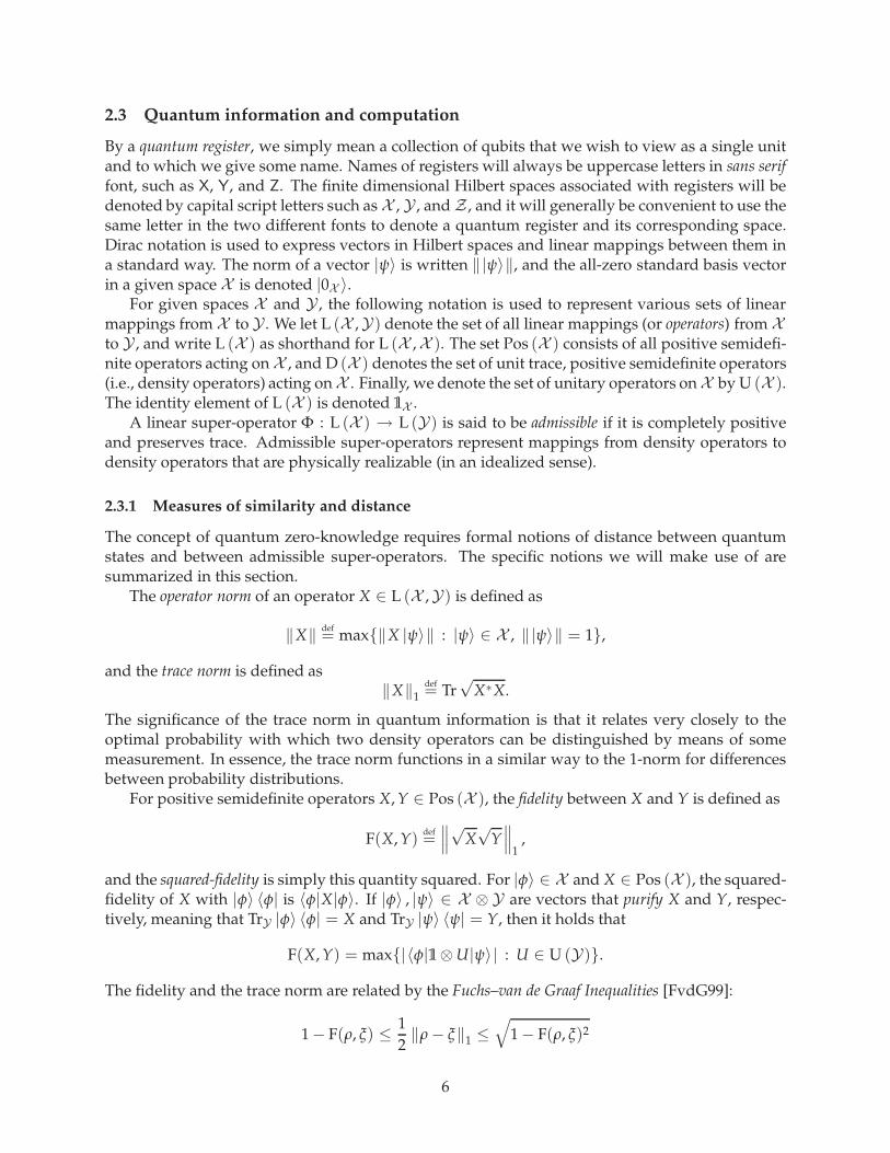
ρ x

PV ′

Φx(ρ)

ρ x

SV′

Ψx(ρ)

Figure 1: Themapping Φx is induced by the actual interaction between P andV ′, and themappingΨx is induced by the simulator alone.

immediately upon being touched by P. In other words, a classical prover P effectively measuresimmediately all qubits received from V ′ with respect to the standard basis.

A simulator SV′ for a given verifier V ′ is described by a polynomial-time generated family ofgeneral quantum circuits that agrees with V ′ on the numbers n and m representing the number ofauxiliary input qubits and output qubits respectively. Such a simulator does not interact with P,but simply induces an admissible operation that we will denote by Ψx : L (W) → L (Z) on eachinput x.

Figure 1 illustrates the two mappings Φx and Ψx. Informally speaking, (V, P) is a quantumzero-knowledge interactive proof system for A if the two mappings Φx and Ψx are indistinguish-able for every choice of x ∈ Ayes. As in the classical case, different notions of indistinguishabil-ity give rise to different variants of zero-knowledge. We will consider quantum statistical zero-knowledge and quantum computational zero-knowledge in the subsections that follow.

3.2 Quantum statistical zero-knowledge

The simpler variant of quantum zero-knowledge is quantum statistical zero-knowledge, which isdefined as follows.

Definition 1. An interactive proof system (V, P) for a promise problem A is quantum statisticalzero-knowledge if it holds that, for every polynomial-time generated quantum verifier V ′, there ex-ists a polynomial-time generated quantum simulator SV′ that satisfies the following requirements.

1. The verifier V ′ and simulator SV′ agree on the polynomially bounded functions q and r thatspecify the number of auxiliary input qubits and output qubits, respectively.

2. Let Φx be the admissible super-operator that results from the interaction between V ′ andP on input x, and let Ψx be the admissible super-operator induced by the simulator SV′

on input x, both as described above. Then there exists a negligible function δ such that‖Φx − Ψx‖⋄ < δ(|x|) for all x ∈ Ayes.

This definition is intended to be completely analogous to the classical definition. By referringto the diamond norm, it implicitly takes into account the fact that the input to Φx and Ψx could

9

be entangled to an external system (which happens to not be a concern in the classical setting).In operational terms, the definition implies that if (i) a pair of quantum registers (W,Y), with Y

an arbitrary external register and W the register containing the auxiliary input to Φx or Ψx, isinitialized to any state ρ, and (ii) one of the mappings Φx or Ψx is applied to W, yielding a newregister Z, then the two possible resulting states of (Z,Y) will have negligible trace distance. Con-sequently, any measurement of the registers would then result in distributions having negligiblestatistical difference. By the triangle inequality, a similar statement holds for any procedure thatis permitted to apply either Φx or Ψx a polynomial number of times, interleaved with arbitraryadmissible operations. In short, the definition means that no physical process can distinguishthe two boxes shown in Figure 1 with a non-negligible bias without making a super-polynomialnumber of queries.

It is necessary to include the possibility of an external system Y if one desires a cryptograph-ically sound definition. For instance, it is possible to define admissible super-operators Φ and Ψ

such that ‖Φ(ρ) − Ψ(ρ)‖1 is strictly smaller than ‖Φ − Ψ‖⋄ for all ρ ∈ D (W) [KSV02]. Indeed,it is possible to define admissible super-operators Φ and Ψ such that ‖Φ(ρ) − Ψ(ρ)‖1 is exponen-tially small (in the number of input and output qubits) for all states ρ ∈ D (W), but for which‖Φ − Ψ‖⋄ = 2, implying that an external system Y that is initially entangled with W allows thetwo mappings to be perfectly distinguished. One can imagine natural situations in which poten-tial attacks on zero-knowledge proofs could be based on this principle.

3.3 Quantum computational indistinguishability and zero-knowledge

A quantum variant of computational zero-knowledge requires a formal notion of quantum com-putational indistinguishability of admissible super-operators. We discuss this notion in this sec-tion, as well as the closely related notion of quantum computational indistinguishability of states.This second notion will also be important later in the context of quantum computationally con-cealing commitment schemes.

The reader should be alerted to the fact that our definitions of quantum computational indis-tinguishability will be very strict, in that they allow polynomial-size quantum circuits to rely onan arbitrary auxiliary quantum state to aid them in distinguishing between two possibilities. Thisis required for the standard proofs of security that we adapt to the quantum setting. The trueimportance of the distinction between this notion of indistinguishability and one not allowing forsuch auxiliary states is an interesting topic, but is not considered further in this paper.

3.3.1 Distinguishability of states

We begin with a definition that quantifies computational distinguishability between states.

Definition 2. Let ρ and ξ bem-qubit mixed states. Then ρ and ξ are said to be (s, k, ε)-distinguishableif there exists a mixed state σ on k qubits and an (m+ k)-qubit quantummeasurement circuit Q ofsize s, such that

|Pr[Q(ρ ⊗ σ) = 1] − Pr[Q(ξ ⊗ σ) = 1]| ≥ ε.

If ρ and ξ are not (s, k, ε)-distinguishable then they are (s, k, ε)-indistinguishable.

Notice that this definition gives a strong quantum analogue to the typical non-uniform notionof classical polynomial indistinguishability. It is strong because the non-uniformity includes anarbitrary quantum state σ that may aid some circuit Q in the task of distinguishing ρ from ξ.The inclusion of the arbitrary state σ is important in the situation we will consider in the context

10

of zero-knowledge, where indistinguishability of quantum states must hold in the presence ofauxiliary quantum information.

Based on the previous definition, we now specify what it means for two ensembles of states tobe quantum computationally indistinguishable.

Definition 3. Assume that S ⊆ Σ∗ is an infinite set of strings, r is a polynomially boundedfunction, and ρx and ξx are mixed states on r(|x|) qubits for each x ∈ S. Then the ensembles{ρx : x ∈ S} and {ξx : x ∈ S} are polynomially quantum indistinguishable if, for every choice ofpolynomially bounded functions p, s, and k, it holds that ρx and σx are (s(|x|), k(|x|), 1/p(|x|))-indistinguishable for all but finitely many x ∈ S.

If {ρn : n ∈ N} and {ξn : n ∈ N} are ensembles indexed by the natural numbers, weidentify S with 1∗, interpreting each n with its unary representation. Let us also note explicitlythat the above definition includes the situation that classical probabilistic ensembles are to bedistinguished. This corresponds to the case where the collections {ρx : x ∈ S} and {ξx : x ∈ S}are diagonal with respect to the standard basis.

It is convenient at this point to state and prove a simple fact concerning the distinguishabilityof states. It will not be used until later in the paper.

Proposition 4. Suppose that ρ1, . . . , ρn and ξ1, . . . , ξn are m-qubit states such that ρ1 ⊗ · · · ⊗ ρn andξ1 ⊗ · · · ⊗ ξn are (s, k, ε)-distinguishable. Then there exists at least one choice of j ∈ {1, . . . , n} for whichρj and ξ j are (s, (n− 1)m + k, ε/n)-distinguishable.

Proof. The proposition is trivial if n = 1, so let us assume n ≥ 2. Let Q be an (nm + k)-qubitmeasurement circuit of size s, and let σ be a k-qubit state, such that

|Pr[Q(ρ1 ⊗ · · · ⊗ ρn ⊗ σ) = 1] − Pr[Q(ξ1 ⊗ · · · ⊗ ξn ⊗ σ) = 1]| ≥ ε.

For each j ∈ {1, . . . , n}, define

δj =∣

∣

∣Pr[Q(ρ1 ⊗ · · · ⊗ ρj ⊗ ξ j+1 ⊗ · · · ⊗ ξn ⊗ σ) = 1]

− Pr[Q(ρ1 ⊗ · · · ⊗ ρj−1 ⊗ ξ j ⊗ · · · ⊗ ξn ⊗ σ) = 1]∣

∣

∣.

It is clear that Q is a measurement circuit that δj-distinguishes ρj and ξ j by means of the auxiliarystate

ρ1 ⊗ · · · ⊗ ρj−1 ⊗ ξ j+1 ⊗ · · · ⊗ ξn ⊗ σ

for each choice of j. By the triangle inequality we have

n

∑j=1

δj ≥ ε

and thus δj ≥ ε/n for at least one choice of j ∈ {1, . . . , n}.

3.3.2 Distinguishability of admissible super-operators

Next we will extend the notion of quantum computational indistinguishability to admissiblesuper-operators.

11

Definition 5. Let Φ and Ψ be admissible super-operators from n qubits to m qubits. These super-operators are said to be (s, k, ε)-distinguishable if there exists a mixed state σ on n + k qubits and an(m + k)-qubit measurement circuit Q of size s such that

|Pr[Q((Φ ⊗ 1k)(σ)) = 1] − Pr[Q((Ψ ⊗ 1k)(σ)) = 1]| ≥ ε.

Here, 1k denotes the identity super-operator on k qubits. If Φ and Ψ are not (s, k, ε)-distinguishablethen they are said to be (s, k, ε)-indistinguishable.

In this definition, it should be viewed that the state σ plays multiple roles: it represents the in-put to the admissible super-operators, allows the possibility of auxiliary qubits that may be entan-gled with the qubits input to Φ or Ψ, and may include additional qubits that aid the measurementcircuit in distinguishing the outputs as in Definition 2.

Again, this definition leads to a notion of quantum computational indistinguishability of ad-missible super-operators as in the following definition.

Definition 6. Assume that S ⊆ Σ∗ is an infinite set of strings, q and r are polynomially boundedfunctions, and Φx and Ψx are admissible super-operators from q(|x|) qubits to r(|x|) qubits foreach x ∈ S. Then the ensembles {Φx : x ∈ S} and {Ψx : x ∈ S} are polynomially quantumindistinguishable if, for every choice of polynomially bounded functions p, s, and k it holds that Φx

and Ψx are (s(|x|), k(|x|), 1/p(|x|))-indistinguishable for all but finitely many x ∈ S.

3.3.3 Definition of quantum computational zero-knowledge

Now we are prepared to state a definition for quantum computational zero-knowledge.

Definition 7. An interactive proof system (V, P) for a promise problem A is quantum computa-tional zero-knowledge if, for every polynomial-time generated quantum verifier V ′, there exists apolynomial-time generated quantum simulator SV′ that satisfies the following requirements.

1. The verifier V ′ and simulator SV′ agree on the polynomially bounded functions q and r thatspecify the number of auxiliary input qubits and output qubits, respectively.

2. Let Φx be the admissible super-operator that results from the interaction between V ′ andP on input x, and let Ψx be the admissible super-operator induced by the simulator SV′ oninput x, both as described above. Then the ensembles {Φx : x ∈ Ayes} and {Ψx : x ∈ Ayes}are polynomially quantum indistinguishable.

3.4 A brief note on closure properties

Similar to the classical case, a sequential composition of quantum zero-knowledge protocols re-sults in a zero-knowledge protocol—a property that again relies on the inclusion of the auxiliaryinput to the verifier. Specifically, the auxiliary input provides a means by which a cheating veri-fier’s memory of previous interactions may be considered during an execution of a given protocol.Along similar lines, the presence of the auxiliary input implies that the classes of promise prob-lems that are quantum statistical zero-knowledge and quantum computational zero-knowledgeare closed under Karp reductions. This fact is discussed in [GMW91] for the classical case, and thequantum and classical settings do not differ in this respect.

In the above definitions we have assumed that the input x is classical. They therefore donot address, for instance, the situation in which one quantum zero-knowledge protocol is run insuperposition inside of another.

12

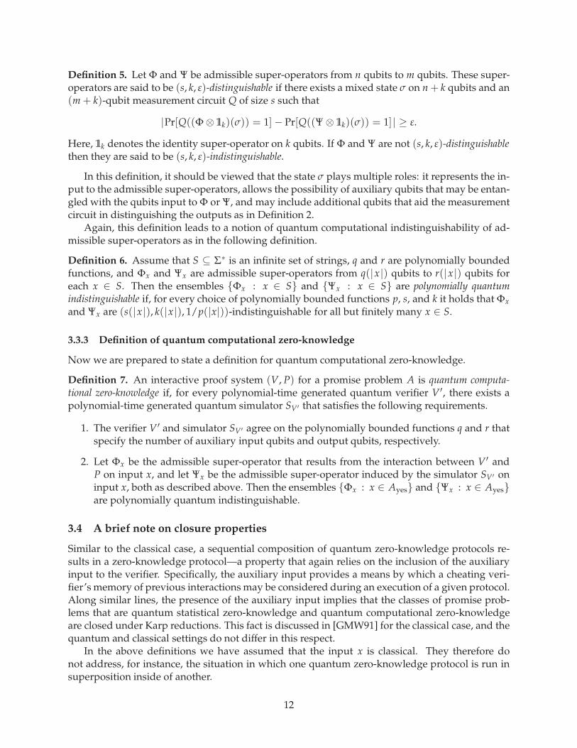
input qubits(initial state is |ψ〉)

ancillary qubits(initial state is |0k〉)

output qubit(measured)

residual qubits(state becomes |φ0(ψ)〉

or |φ1(ψ)〉)

Q

Figure 2: Given circuit Q for Quantum Rewinding Lemma

4 The Quantum Rewinding Lemma

The polynomial-time quantum simulator constructions for the various protocols considered in thispaper rely on theQuantumRewinding Lemma proved in this section. More precisely, two variants oftheQuantumRewinding Lemma are proved: an exact version (Lemma 8) and a version that allowsfor small perturbations (Lemma 9). Both variants concern an abstract computational problem thatwill now be discussed.

Let Q be a unitary quantum circuit acting on n + k qubits. For an arbitrary pure quantumstate |ψ〉 on n qubits, consider the process in which the circuit Q is applied to the state |ψ〉 |0k〉,after which the first qubit is measured with respect to the standard basis. Let p(ψ) denote theprobability that this measurement outcome is 0, and let us assume that p(ψ) is neither 0 nor 1.Under this assumption, there is a unique choice of unit vectors |φ0(ψ)〉 and |φ1(ψ)〉 such that

Q |ψ〉 |0k〉 =√

p(ψ) |0〉 |φ0(ψ)〉 +√

1− p(ψ) |1〉 |φ1(ψ)〉 .

We write |φ0(ψ)〉 and |φ1(ψ)〉 to stress the dependence of these vectors on |ψ〉. These vectorsrepresent the residual state of the n+ k− 1 qubits aside from the first after the measurement takesplace, respective to the measurement outcome. This situation is illustrated in Figure 2.

Now, let us imagine that it is our goal to construct from Q a procedure that takes as inputan arbitrary state |ψ〉 and outputs a state that is as close as possible to |φ0(ψ)〉. The notion ofcloseness that we will focus on is the squared-fidelity between the output state and |φ0(ψ)〉. Notethat by simply running Q on the state |ψ〉 |0k〉 and discarding the first qubit, we of course succeedin producing an output that has squared-fidelity at least p(ψ) with |φ0(ψ)〉; and without furtherassumptions on the circuit Q it may not be possible to do significantly better.

The Quantum Rewinding Lemma establishes a condition on Q that allows for the state |φ0(ψ)〉to be output with any desired fidelity. Specifically, under the assumption that the probability p(ψ)is independent of the state |ψ〉, there exists an efficient procedure that outputs a state having veryhigh fidelity with |φ0(ψ)〉. To achieve fidelity-squared at least 1− ε, the procedure requires

O

(

log(1/ε)

p(1− p)

)

executions of Q and Q∗, interleaved with simple unitary gates and measurements. The QuantumRewinding Lemmawith small perturbations concerns precisely the same procedure under slightlyweaker assumptions.

13

Before stating and proving the Quantum Rewinding Lemma more formally, let us brieflydiscuss the connection between the above problem and the construction of simulators for zero-knowledge protocols. The circuit Qwill represent a “reasonable attempt” to construct a simulatorfor some cheating verifier for some protocol, and the input state |ψ〉 will represent the auxiliaryinput of this verifier. It is very important that Q is unitary, so it is perhaps more accurate to viewQ as being a purification of a “reasonable attempt” to simulate the given verifier. The measure-ment of the first qubit will indicate the success or failure of the simulation, with output 0 mean-ing that the simulation was successful and output 1 indicating that the simulation has failed, sorewinding is necessary. Supposing that the probability of a successful simulation is small but non-negligible, we therefore have that the Quantum Rewinding Lemma establishes a condition underwhich rewinding is possible: if the success probability of our “reasonable attempt” at a simulatoris independent, or nearly independent, of the auxiliary input, then it is possible to generate theoutput corresponding to a successful simulation with very high fidelity.

This property of independence, or near-independence, of the simulator’s success probabilityfrom the auxiliary input could potentially represent an obstacle to applying our method to someprotocols. For the protocols considered in this paper, however, it does not—the most straightfor-ward “reasonable attempts” to construct simulators will easily be shown to have this indepen-dence or near-independence property.

4.1 The exact case

Wewill begin with the Quantum Rewinding Lemma in the exact setting, where it is assumed thatthe measurement outcome in the process described above is completely independent of the inputstate |ψ〉.

For clarity, let us give a name to the type of circuit discussed above; we define an (n, k)-quantumcircuit to be any unitary quantum circuit that acts on n+ k qubits, where the first n qubits may takean arbitrary quantum state |ψ〉 as input and the remaining k qubits are initially set to the state |0k〉.Given such a circuit, the probability p(ψ) and the residual states |φ0(ψ)〉 and |φ1(ψ)〉 are definedas above.

Lemma 8 (Quantum Rewinding Lemma, exact case). Let Q be an (n, k)-quantum circuit, and assumethat p = p(ψ) is constant over all choices of the input |ψ〉 and satisfies p ∈ (0, 1). Then for every ε > 0there is a general quantum circuit R, with

size(R) = O

(

log(1/ε) size(Q)

p(1− p)

)

,

such that for every input |ψ〉, the output ρ(ψ) of R satisfies

〈φ0(ψ)|ρ(ψ)|φ0(ψ)〉 ≥ 1− ε. (1)

Proof. For a given circuit Q and error bound ε, let R be a quantum circuit implementing the pro-cedure described in Figure 3. The size of R can be seen to be as claimed. It therefore remains toprove that the output ρ(ψ) of R on any input |ψ〉 satisfies the required bound (1).

To this end, let us define three projections, each acting on n + k qubits:

Π0 = |0〉 〈0| ⊗ 1, Π1 = |1〉 〈1| ⊗ 1, ∆ = 1 ⊗ |0k〉 〈0k| .

The measurement of the qubit B that is performed in the procedure may be viewed as a mea-surement with respect to the projections {Π0,Π1}, while the phase flip performed in case the

14

Initial conditions:

The register W contains an n-qubit quantum input |ψ〉.The register X is initialized to the state |0k〉.

The procedure:

Set t = 0.

Apply the circuit Q to the pair (W,X) obtaining (B,Y). (The register B represents the outputqubit of Q and the register Y represents the remaining n + k− 1 residual qubits.)

Repeat:

Measure B with respect to the computational basis.

If the outcome of the measurement is 1:

Apply Q∗ to (B,Y), obtaining (W,X).

Perform a phase flip in case any of the qubits of X is set to 1. (Equivalently, apply the

unitary operation 2 |0k〉 〈0k| − 1 to X.)

Apply Q to the pair (W,X) obtaining (B,Y).

Set t = t + 1.

Until the measurement outcome is 0 or t = ⌈log(1/ε)/(4p(1− p))⌉.Output the register Y.

Figure 3: Quantum Rewinding Procedure

measurement result is 1 may be written 2∆ − 1. Let us also define positive semidefinite operatorsP0 and P1 as follows:

P0 = (1 ⊗ 〈0k|)Q∗Π0Q(1 ⊗ |0k〉),P1 = (1 ⊗ 〈0k|)Q∗Π1Q(1 ⊗ |0k〉).

The n-qubit measurement that is effectively performed on the quantum input |ψ〉 when the circuitQ is applied and the output qubit is measured is described as a POVM-type measurement by{P0, P1}.

The assumptions of the lemma imply that for every input state |ψ〉 we have 〈ψ|P1|ψ〉 = 1− p.There is only one possibility for the operator P1 given this fact: it must be that P1 = (1 − p)1.This is because P1, similar to any other linear operator, is uniquely determined by the function|ψ〉 7→ 〈ψ|P1|ψ〉 defined on the unit sphere. Consequently, we have

∆Q∗Π1Q∆ = (1 ⊗ |0k〉)P1(1 ⊗ 〈0k|) = (1− p)∆. (2)

Let us now fix an arbitrary n-qubit quantum input |ψ〉, so that |ψ〉 |0k〉 is the initial state of thepair (W,X) when the procedure described by R is run. After applying Q, we obtain the state

Q |ψ〉 |0k〉 =√p |0〉 |φ0(ψ)〉 +

√

1− p |1〉 |φ1(ψ)〉

in registers (B,Y). A measurement of B with respect to the standard basis now occurs. If themeasurement results in outcome 0, then the residual state of register Y becomes |φ0(ψ)〉 and the

15

procedure is terminated, giving the desired output. If, however, the measurement outcome is 1,then the state of the pair (B,Y) becomes |1〉 |φ1(ψ)〉. The operations that are performed in this casetransform the state of the pair (B,Y) to

Q(2∆ − 1)Q∗ |1〉 |φ1(ψ)〉 .

Using the above equation (2) along with the observation ∆ |ψ〉 |0k〉 = |ψ〉 |0k〉, we may nowcalculate:

Q(2∆ − 1)Q∗ |1〉 |φ1(ψ)〉 =1

√

1− pQ(2∆ − 1)Q∗Π1Q∆ |ψ〉 |0k〉

= 2√

1− p Q |ψ〉 |0k〉 − 1√

1− pΠ1Q |ψ〉 |0k〉

= 2√

p(1− p) |0〉 |φ0(ψ)〉 + (1− 2p) |1〉 |φ1(ψ)〉 .

This equation, which establishes that the vector

Q(2∆ − 1)Q∗ |1〉 |φ1(ψ)〉

lies in the two-dimensional space spanned by |0〉 |φ0(ψ)〉 and |1〉 |φ1(ψ)〉, is the key to the proof.Figure 4 illustrates the relationship among the relevant vectors. It should be stressed that this factrelies critically on the assumption that p(ψ) is constant over all choices of |ψ〉.

We now see that a measurement of B at this point results in outcome 0 and correspondingresidual state |φ0(ψ)〉 with probability 4p(1− p), and outcome 1 and residual state |φ1(ψ)〉 withprobability (1− 2p)2. For each subsequent iteration of the loop, which is only performed in casethe measurement outcome was 1, the pattern is identical. Consequently, whenever the measure-ment outcome is 0, the output of the procedure is |φ0(ψ)〉, and the probability that the measure-ment outcome is 0 within t iterations is

1− (1− p)(1− 2p)2t .

The probability that |φ0(ψ)〉 is output by the procedure is therefore greater than 1− ε if at least

log(1/ε)

4p(1− p)

iterations of the loop are permitted, which implies the required bound (1).

A preliminary version of the present paper contained a somewhat less direct proof of the abovelemma, based on the QMA error reduction technique presented in Marriott and Watrous [MW05].Another proof has been suggested by Oded Regev [Reg06], based on the notion of angles betweensubspaces developed by Jordan [Jor75]. (Section VII.1 of Bhatia [Bha97] includes an extensivediscussion of this notion.)

4.1.1 Relationship to Grover’s Algorithm

It will be clear to some readers that the Quantum Rewinding Procedure described in Figure 3has some resemblance to Grover’s Algorithm [Gro96, Gro97, BBHT98] and the process known asAmplitude Amplification [BHMT02]. Specifically, if the measurement of B were replaced with a

16

θθ

|1〉 |φ1(ψ)〉

|0〉 |φ0(ψ)〉

√p |0〉 |φ0(ψ)〉 +

√

1− p |1〉 |φ1(ψ)〉

Q(2∆ − 1)Q∗ |1〉 |φ1(ψ)〉

Figure 4: The action of Q(2∆ − 1)Q∗ on |1〉 |φ1(ψ)〉. The angle between the vectors |1〉 |φ1(ψ)〉 andQ(2∆ − 1)Q∗ |1〉 |φ1(ψ)〉 is twice the angle θ = sin−1(

√p).

phase-flip 2Π0 − 1, the resulting algorithm could reasonably be described as performing Ampli-tude Amplification with a quantum state input. Naturally, if there are no measurements withinthe loop, then the number of iterations of the loop that are performed must be determined bysome other means. This approach has been investigated within the context of zero-knowledge byMatsumoto [Mat06].

It should be noted, however, that there are two fundamental differences between the QuantumRewinding Procedure and Grover’s Algorithm/Amplitude Amplification. The first major differ-ence is of course that the Quantum Rewinding Procedure takes a quantum state input whereas,to the knowledge of the author, this has not been considered in the case of Grover’s Algorithm orAmplitude Amplification. The requirement that p(ψ) is constant over all input states |ψ〉, whichhas paramount importance in the above analysis, is obviously vacuous when there is no quantumstate input.

The second difference is that, in the interest of simplicity, the Quantum Rewinding Procedurecompletely sacrifices the speed-up that represents the key feature of Grover’s Algorithm and Am-plitude Amplification. It has been argued above that the output of the procedure satisfies therequired bound (1) and runs in polynomial time, even for exponentially small ε. When we applythe Quantum Rewinding Lemma to the construction of simulators for zero-knowledge protocols,it will be necessary that ε can be chosen to be negligible. If, however, we were to replace themeasurement of B within the loop with a phase-flip in an attempt to mimic the behavior of Am-plitude Amplification, it would be necessary in the general case to make further modificationsto the procedure to guarantee the required bound (1). This could presumably be done using thetechniques of [BHMT02], but the procedure would likely be significantly more complicated thanthe one described above.

A study of Amplitude Amplification with a quantum state input has the potential to be bothinteresting and useful. However, in the context of constructing zero-knowledge simulators thismethod has limited appeal. This is because a simulator for a zero-knowledge protocol is doingsomething that is useless by assumption—it acts only as a reduction, establishing that a given verifiermust fail to extract knowledge from the honest prover. It therefore does not seem worthwhile to

17

optimize simulators, or to sacrifice their simplicity in the interest of the quadratic speed-up thatcould be offered by Amplitude Amplification.

4.2 Quantum rewinding with small perturbations

The assumptions of Lemma 8 require that p is independent of |ψ〉. Here we note that this assump-tion may be relaxed slightly if one is willing to accept a small perturbation in the output of theprocedure.

Lemma 9 (Quantum Rewinding Lemma with small perturbations). Let Q be an (n, k)-quantumcircuit and let p0, q ∈ (0, 1) and ε ∈ (0, 1/2) be real numbers such that

1. |p(ψ) − q| < ε,

2. p0(1− p0) ≤ q(1− q), and

3. p0 ≤ p(ψ)

for all n-qubit states |ψ〉. Then there exists a general quantum circuit R with

size(R) = O

(

log(1/ε) size(Q)

p0(1− p0)

)

such that, for every n-qubit state |ψ〉, the output ρ(ψ) of R satisfies

〈φ0(ψ)|ρ(ψ)|φ0(ψ)〉 ≥ 1− 16εlog2(1/ε)

p20(1− p0)2. (3)

Readers not interested in the technical details of the proof of this lemma may be satisfied bythe following brief summary of the proof, whose main idea is very simple. A given circuit Q maynot satisfy the requirements of Lemma 8, but if it satisfies the weaker assumptions of Lemma 9,then Q must induce a unitary operation that is close (in operator norm) to a unitary operator Uthat does satisfy the requirements of Lemma 8. We then consider precisely the same circuit R thatis described in the proof of Lemma 8, except with p0 replacing p. The bound given by Lemma 9 isobtained from the one of Lemma 8 together with an analysis of the possible difference that couldresult by substituting U for Q in the circuit R.

Proof. The circuit construction for R is identical to the Quantum Rewinding Procedure given inthe proof of Lemma 8, except that p0 is substituted for p. The size of R is therefore as claimed, soit remains to prove that the stated bound (3) holds.

Let {|ψ1〉 , . . . , |ψ2n〉} be an orthonormal basis consisting of eigenvectors of the operator

(1 ⊗ 〈0k|)Q∗Π0Q(1 ⊗ |0k〉).

We will assume hereafter that a general input state |ψ〉 is given by

|ψ〉 =2n

∑i=1

αi |ψi〉 .

The equation

Q |ψ〉 |0k〉 =√

p(ψ) |0〉 |φ0(ψ)〉 +√

1− p(ψ) |1〉 |φ1(ψ)〉

18

therefore implies that

|φ0(ψ)〉 =2n

∑i=1

αi

√

p(ψi)

p(ψ)|φ0(ψi)〉 and |φ1(ψ)〉 =

2n

∑i=1

αi

√

1− p(ψi)

1− p(ψ)|φ1(ψi)〉 .

Now, given that

Π0Q(1 ⊗ |0k〉) |ψi〉 =√

p(ψi) |0〉 |φ0(ψi)〉for i = 1, . . . , 2n, we have that

0 = 〈ψi| (1 ⊗ 〈0k|)Q∗Π0Q(1 ⊗ |0k〉) |ψj〉 =√

p(ψi)p(ψj) 〈φ0(ψi)|φ0(ψj)〉

for i 6= j. It follows that the set {|φ0(ψ1)〉 , . . . , |φ0(ψ2n)〉} is orthonormal. By similar reasoning{|φ1(ψ1)〉 , . . . , |φ1(ψ2n)〉} is orthonormal as well.

These orthonormality relations allow us to define a unitary operator U that is close to Q andsatisfies the requirements of Lemma 8. Specifically let us defineU = VQ, where V is the uniquelydetermined unitary operator that satisfies the equations

V

(

√

p(ψi) |0〉 |φ0(ψi)〉 +√

1− p(ψi) |1〉 |φ1(ψi)〉)

=√q |0〉 |φ0(ψi)〉+

√

1− q |1〉 |φ1(ψi)〉 ,

V

(

√

1− p(ψi) |0〉 |φ0(ψi)〉 −√

p(ψi) |1〉 |φ1(ψi)〉)

=√

1− q |0〉 |φ0(ψi)〉 −√q |1〉 |φ1(ψi)〉 ,

for i = 1, . . . , 2n, and acts trivially on the orthogonal complement to the subspace spanned by

{|0〉 |φ0(ψ1)〉 , . . . , |0〉 |φ0(ψ2n)〉 , |1〉 |φ1(ψ1)〉 , . . . , |1〉 |φ1(ψ2n)〉} .

It is clear that

‖Q−U‖ ≤ max1≤i≤2n

√

(

√

p(ψi) −√q

)2

+

(

√

1− p(ψi) −√

1− q

)2

<

√2ε.

Next, consider the effect of replacing Q by U in the circuit R. Let us denote by ξ(ψ) the outputof R when this replacement is made on input |ψ〉. We have that

U |ψi〉 |0k〉 =√q |0〉 |φ0(ψi)〉 +

√

1− q |1〉 |φ1(ψi)〉

for all choices of i, and therefore

U |ψ〉 |0k〉 =√q |0〉 |δ0(ψ)〉 +

√

1− q |1〉 |δ1(ψ)〉

for

|δ0(ψ)〉 =2n

∑i=1

αi |φ0(ψi)〉 and |δ1(ψ)〉 =2n

∑i=1

αi |φ1(ψi)〉 .

Given that p0(1− p0) ≤ q(1− q), we conclude from Lemma 8 that

〈δ0(ψ)|ξ(ψ)|δ0(ψ)〉 ≥ 1− ε. (4)

It is convenient at this point to make use of a notion of distance known as the fidelity distance.This distance is defined by

dF(σ, τ)def= min{‖|η〉 − |µ〉‖ : |η〉 and |µ〉 purify σ and τ, respectively} =

√

2− 2 F(σ, τ).

19

This is a proper notion of distance: it is symmetric, positive definite, and the triangle inequalityholds [KSV02]. We will prove bounds on three quantities:

dF(ρ(ψ), ξ(ψ)),

dF(ξ(ψ), |δ0(ψ)〉 〈δ0(ψ)|),

anddF(|δ0(ψ)〉 〈δ0(ψ)| , |φ0(ψ)〉 〈φ0(ψ)|).

The triangle inequality will therefore imply that the quantity dF(ρ(ψ), |φ0(ψ)〉 〈φ0(ψ)|) is at mostthe sum of these three quantities. The equation F(σ, τ)2 ≥ 1− dF(σ, τ)2, which is easily shown tohold for any choice of density operators σ and τ, will then yield the required bound (3).

Let us begin with a bound on dF(ρ(ψ), ξ(ψ)). The fidelity distance between these two densityoperators is no larger than the Euclidean distance between two purifications of our choice—so wemay choose purifications that arise from running a purification of the circuit R. Given that thetotal number of times that either of Q or Q∗ is applied during the execution of R is 2t + 1, where

t =

⌈

log(1/ε)

4p0(1− p0)

⌉

,

the distance between the two purifications in question is at most (2t + 1) ‖Q−U‖. Thus we have

dF(ρ(ψ), ξ(ψ)) ≤ (2t + 1) ‖Q−U‖ ≤ (2t + 1)√2ε. (5)

Next, we wish to bound the quantity dF(ξ(ψ), |δ0(ψ)〉 〈δ0(ψ)|). It follows from the above equa-tion (4) that

dF(ξ(ψ), |δ0(ψ)〉 〈δ0(ψ)|) ≤√2ε. (6)

Finally, the quantity dF(|δ0(ψ)〉 〈δ0(ψ)| , |φ0(ψ)〉 〈φ0(ψ)|) is equal to the Euclidean distance be-tween the vectors |δ0(ψ)〉 and |φ0(ψ)〉. As

‖|δ0(ψ)〉 − |φ0(ψ)〉‖2 =2n

∑i=1

|αi |2(

1−√

p(ψi)

p(ψ)

)2

≤ 2ε

p0,

we have

dF(|δ0(ψ)〉 〈δ0(ψ)| , |φ0(ψ)〉 〈φ0(ψ)|) ≤√

2ε

p0. (7)

By combining the above equations (5), (6), and (7) by means of the triangle inequality, we have

dF(ρ(ψ), |φ0(ψ)〉 〈φ0(ψ)|) ≤(

2t + 2+1√p0

)√2ε ≤ 4 log(1/ε)

p0(1− p0)

√ε.

Therefore

〈φ0(ψ)|ρ(ψ)|φ0(ψ)〉 ≥ 1− 16εlog2(1/ε)

p20(1− p0)2

as claimed.

The bound given in the statement of the above lemma is clearly not tight—some precision issacrificed in order to obtain a simpler expression. The lemmawill later be used in the situation thatε is negligible, but where p0(1− p0) is not. The conclusion in this case is that the state producedby R has fidelity 1 minus some negligible quantity with the desired state |φ0(ψ)〉.

20

Zero-Knowledge Protocol for Graph Isomorphism

The input is a pair (G0,G1) of simple, undirected n-vertex graphs. It is assumed that the proverknows a permutation σ ∈ Sn that satisfies σ(G1) = G0 if G0 and G1 are isomorphic.

Prover’s step 1: Choose π ∈ Sn uniformly at random and send H = π(G0) to the verifier.

Verifier’s step 1: Choose a ∈ Σ uniformly at random and send a to the prover. (Implicitly, theverifier is challenging the prover to exhibit an isomorphism between Ga and H.)

Prover’s step 2: Set τ = πσa and send τ to the verifier. (If σ(G1) = G0, then τ(Ga) = H.)

Verifier’s step 2: Accept if τ(Ga) = H, reject otherwise.

Figure 5: The Goldreich–Micali–Wigderson Graph Isomorphism protocol.

5 Quantum statistical zero-knowledge proof systems

The Goldreich–Micali–Wigderson Graph Isomorphism protocol is a simple and well-known ex-ample of an interactive proof system that is perfect (and therefore statistical) zero-knowledgeagainst classical polynomial-time verifiers. The question of whether this protocol remains zero-knowledge against quantum verifiers was the starting point of the research in the present paper,and so it is fitting to illustrate our technique by first considering this protocol. Section 5.1 dis-cusses this protocol and contains a proof that it indeed remains zero-knowledge against quantumverifiers.

The Goldreich–Micali–Wigderson protocol for Graph Isomorphism has a simple form:

1. The prover sends a message to the verifier,

2. the verifier flips a single coin and sends the result to the prover, and

3. the prover responds with a second message. The verifier then decides to accept or rejectbased on the three messages exchanged.

Protocols of this form are amenable to analysis in the quantum setting by means of the QuantumRewinding Lemma of the previous section, provided certain assumptions are met. These assump-tions translate to the independence of p from |ψ〉 in Lemma 8. In the quantum setting, protocolsof this simple form are universal for honest-verifier quantum statistical zero-knowledge [Wat02],meaning that every problem having a quantum interactive proof system that is statistical zero-knowledge with respect to an honest verifier also has a proof system of the above form. Thisleads to a proof, discussed in Section 5.2, that honest verifier and general quantum statistical zero-knowledge interactive proof systems are equivalent with respect to computational power.

5.1 Graph isomorphism

Figure 5 describes the Goldreich–Micali–Wigderson Graph Isomorphism protocol [GMW91].The corresponding interactive proof system has perfect completeness and soundness error

1/2; if G0∼= G1, then the verifier V will accept with probability 1 when interacting with the honest

21

prover P, while if G0 6∼= G1 then no prover P′ can convinceV to accept with probability greater than1/2 (essentially because the graph H sent by the prover in the first message cannot be isomorphicto both G0 and G1 when G0 6∼= G1).

For any choice of σ ∈ Sn that satisfies the required property σ(G1) = G0 for G0∼= G1, the

interactive proof system (V, P) is perfect zero-knowledgewith respect to any classical polynomial-time verifier V ′. Sequential repetition followed by a unanimous vote can be used to decrease thesoundness error to an exponentially small quantity while preserving the perfect completeness andclassical zero-knowledge properties.

Our goal to prove this protocol is zero-knowledge with respect to polynomial-time quantumverifiers. It will be sufficient to consider a restricted type of verifier as follows:

1. In addition to (G0,G1), the verifier takes a quantum register W as input, representing theauxiliary quantum input. The verifier will use two additional quantum registers that func-tion as work space: V, which is an arbitrary (polynomial-size) register, and A, which is asingle qubit register. The registers V and A are initialized to their all-zero states before theprotocol begins.

2. In the first message, the prover P sends an n-vertex graph H to the verifier. For each graphH there corresponds a unitary operator V ′

H that the verifier applies to the registers (W,V,A).After applying the appropriate operation V ′

H, the verifier measures the register A with re-spect to the standard basis, and sends the resulting bit a to the prover.

3. After the prover responds with some permutation τ ∈ Sn, the verifier simply outputs theregisters (W,V,A), along with the classical messages H and τ sent by the prover during theprotocol.

Any polynomial-time quantum verifier can be modeled as a verifier of this restricted formfollowed by some polynomial-time post-processing of the restricted verifier’s output. The samepost-processing can be applied to the output of the simulator that will be constructed for thegiven restricted verifier. Notice that a verifier of this restricted form is completely determined bythe collection {V ′

H}.Now let us consider the admissible super-operator induced by an interaction of a verifier of

the above type with the prover P in the case that G0∼= G1. Although the messages sent from the

prover to the verifier are classical messages, it will simplify matters to view them as being storedin quantum registers denoted P1 and P2, respectively. Later, when we consider simulations of theinteraction, we will need quantum registers to store these messages anyway, and it is helpful tohave the registers used in the actual protocol and in the simulation share the same names.

Let us write Gn to denote the set of all simple, undirected graphs having vertex set {1, . . . , n}.For each H ∈ Gn and each a ∈ Σ, define a linear mapping

MH,a = (1W⊗V ⊗ 〈a|)V ′H(1W ⊗ |0V⊗A〉)

fromW toW ⊗V . If the initial state of the register W is a pure state |ψ〉 ∈ W , then the state of theregisters (W,V,A) after the verifier applies V ′

H is

(MH,0 |ψ〉) |0〉 + (MH,1 |ψ〉) |1〉 ,

and therefore the state of the registers (W,V,A) after the verifier applies V ′H and measures A with

respect to the standard basis is

∑a∈Σ

MH,a |ψ〉 〈ψ|M∗H,a ⊗ |a〉 〈a| .

22

The admissible super-operator that results from the interaction is now easily described by incor-porating the description of P. It is given by

Φ(X) =1

n! ∑π∈Sn

∑a∈Σ

Mπ(G0),aXM∗π(G0),a

⊗ |a〉 〈a| ⊗ |π(G0)〉 〈π(G0)| ⊗ |πσa〉 〈πσa| (8)

for all X ∈ L (W).In order to define a simulator for a given quantum verifier V ′, it is helpful to consider the

classical case. A classical simulation for a classical verifier in the above protocol may be obtainedas follows. The simulator randomly chooses a permutation π and a bit b, and feeds π(Gb) to theverifier. This verifier chooses a bit a for its message back to the prover. If a = b, the simulatorcan easily complete the simulation, otherwise it rewinds and tries a new choice of π and b. Withvery high probability, the simulator will succeed after no more than a polynomial number ofsteps, given that the event a = b must happen with probability exactly 1/2 (regardless of theverifier’s actions). In case of success, the output of the simulator and the verifier will be identicallydistributed.

Our simulator for a quantum verifier proceeds along similar lines, except that we must invokethe Quantum Rewinding Lemma instead of ordinary classical rewinding. Our procedure willrequire two registers B and R in addition to W, V, A, P1, and P2. The register R may be viewedas a quantum register whose basis states correspond to the possible random choices that a typicalclassical simulator would use. In the present case this means a random permutation together witha random bit. The register B will represent the simulator’s “guess” for the verifier’s message. Forconvenience, let us define E = V ⊗A⊗Y ⊗ B ⊗Z ⊗R, which is the space corresponding to thecollection of all registers aside from W.

The procedure will involve a composition of a few operations that we now describe. First, letT be any unitary operator acting on registers (P1,B,P2,R) that maps the initial all-zero state ofthese four registers to the state

1√2n!

∑b∈Σ

∑π∈Sn

|π(Gb)〉 |b〉 |π〉 |π, b〉 .

If the register R is traced out, the state of registers (P1,B,P2) corresponds to a probability distribu-tion over triples (π(Gb), b,π) for b and π chosen uniformly. In essence, T produces a purificationof a uniform distribution of possible transcripts of an interaction between a prover and verifier.

Next, define a unitary operator V ′ acting on registers (W,V,A,P1) that effectively simulates(unitarily) the verifier V ′. Specifically, V ′ uses P1 as a control register, and applies V ′

H to regis-ters (W,V,A) for each possible graph H ∈ Gn representing a standard basis state of P1. Morecompactly,

V ′ = ∑H∈Gn

V ′H ⊗ |H〉 〈H| .

The operators T and V ′ are each tensoredwith the identity on the remaining spaces when we wishto view them both as operators onW ⊗ E .

Now consider the quantum circuit Q acting on all of the above registers that is obtained byfirst applying T, then applying V ′, and finally performing a controlled-NOT operation on thepair (A,B) with A acting as the control. Suppose that Q is applied to |ψ〉 |0E 〉, and the registerB is then measured with respect to the standard basis. The probability that the outcome is 0 isnecessarily equal to 1/2, independent of the behavior of the verifier V ′ and of the auxiliary input|ψ〉. This follows from similar reasoning to the classical case: there can be no correlation between

23

the verifier’s choice of a and the simulator’s guess b for a because each graph H is equally likelyto be derived from G0 as G1. If we condition on the measurement outcome being 0, and trace outthe register R, we obtain precisely the admissible super-operator Φ given in Eq. (8) describing theactual interaction between V ′ and P. In other words, conditioned on the measurement outcomebeing 0, the circuit Q correctly simulates the interaction between V ′ and P given auxiliary input|ψ〉.

Given that the measurement outcome is 0 with probability 1/2, which is independent of |ψ〉,we may apply Lemma 8 in order to obtain a circuit R. This circuit R, followed by the partial traceover R, represents the final simulation procedure.

Notice that because we are in the special case where p = 1/2, the simulation procedure infact works perfectly after either zero or one iterations of the loop in the Quantum RewindingProcedure. This establishes that the outcome of the simulation procedure is precisely Φ(|ψ〉 〈ψ|) incase the initial state of W was |ψ〉. This may be viewed as an improvement over the classical case,where it is not known if a perfect simulation is possible in worst-case polynomial time.

Because the set {|ψ〉 〈ψ| : |ψ〉 ∈ W , ‖|ψ〉‖ = 1} spans all of L (W), and the super-operatorinduced by the simulation procedure is necessarily admissible (and therefore linear), it holds thatthis map is precisely Φ. In other words, because admissible super-operators are uniquely deter-mined by their action on pure states, the super-operator induced by the simulation proceduremust be Φ; the simulation procedure implements exactly the same admissible super-operator asthe actual interaction between V and P.

Each of the operations constituting the circuit Q can be performed by polynomial-size circuits,and therefore the simulator has polynomial size (in the worst case).

5.2 Honest versus general verifier QSZK

We now consider a quantum interactive proof system for a complete promise problem for the classQSZKHV. This is the class of problems having honest verifier quantum statistical zero-knowledgeinteractive proof systems. This interactive proof system has the same three-message form as theGoldreich–Micali–Wigderson Graph Isomorphism protocol, wherein the verifier’s message is asingle classical coin-flip. In this case, the prover’s messages will be quantum.

Of course it is not the case that every protocol of the above form is zero-knowledge. However,the similarities between the Graph Isomorphism protocol and the protocol for QSZKHV to be con-sidered are sufficient to admit a similar analysis in terms of quantum attacks. This fact allows us toconclude that honest and general verifier quantum statistical zero-knowledge are computationallyequivalent.

5.2.1 Definition of honest verifier quantum statistical zero-knowledge

Let us begin with some definitions that formalize the notion of an honest verifier. We will notrequire these definitions; they are only included for the sake of completeness. Further informationabout these definitions can be found in [Wat02].

Definition 10. Suppose that r is a polynomially bounded function and {ρx} is a collection of quan-tum states, where each ρx is a state on r(|x|) qubits. This collection is said to be polynomial-timepreparable if there exists a polynomial-time uniformly generated family {Qx} of general quantumcircuits such that each circuit Qx takes no inputs, has r(|x|) output qubits, and results in the stateρx when run.

24

Definition 11. Let (V, P) be a quantum interactive protocol forwhichV is described by a collectionof unitary circuits. Define viewV,P(x, j) to be the reduced state of the verifier and message qubitsafter j messages have been sent during an execution of the protocol on input x. The pair (V, P) isan honest verifier quantum statistical zero-knowledge interactive proof system for a promise problem A if:

1. (V, P) is a quantum interactive proof system for A, and

2. there exists a polynomial-time preparable set {σx,j} and a negligible function δ such that

‖σx,j − viewV,P(x, j)‖tr < δ(|x|)

for every x ∈ Ayes and each message number j.

We denote by QSZKHV the class of all promise problems having honest verifier quantumstatistical zero-knowledge interactive proof systems with completeness and soundness error atmost 1/3.

5.2.2 Equivalence of honest and general verifier quantum statistical zero-knowledge

Denote by QSZK the class of promise problems having quantum statistical zero-knowledge inter-active proof systems with completeness and soundness error at most 1/3. We will now prove thatQSZK = QSZKHV by making use of some results proved in [Wat02].

First, define the ε-Close Quantum States problem as follows.

ε-Close Quantum States

Input: General quantum circuits Q0 and Q1, both having no input qubits and m out-put qubits. Let ρ0 and ρ1 denote the states obtained by running Q0 and Q1,respectively.

Yes: ‖ρ0 − ρ1‖1 < ε.

No: ‖ρ0 − ρ1‖1 > 2− ε.

One may consider ε to be a fixed constant or a function of the size of the description of Q0 andQ1, with each choice giving rise to a different promise.

The ε-Close Quantum States problem is complete for QSZKHV for a fairly wide range of choicesfor ε. One specific fact that results and is well suited to our needs is as follows.

Theorem 12. Every promise problem A ∈ QSZKHV Karp-reduces to an instance of the ε-Close QuantumStates problem for which ε is a negligible function of the input size.

Finally, let us recall that the protocol described in Figure 6 is an interactive proof system forε-Close Quantum Stateswith completeness error bounded by ε/2 and soundness error bounded by1/2 +

√ε/2. Sequential repetition followed by a unanimous vote results in negligible bounds for

both completeness and soundness errors.Now, with these facts in hand, we are ready to prove the main result of this subsection.

Theorem 13. QSZK = QSZKHV.

25

Zero-Knowledge Protocol for ε-Close Quantum States

Let R0 and R1 be unitary circuit purifications of Q0 and Q1, respectively. Assume that the circuitsR0 and R1 both act on m + k qubits, with one of the circuits padded with extra unused ancillaryqubits if necessary.

Prover’s step 1: Apply R0 to |0m+k〉 and send the first m qubits to the verifier.

Verifier’s step 1: Choose a ∈ Σ uniformly at random and send a to the prover.

Prover’s step 2: Let U be a unitary operator on k qubits such that

〈0m+k|R∗1(1 ⊗U)R0|0m+k〉 = F(ρ0, ρ1).

If a = 1, apply the unitary operationU to the residual qubits of R0 that were not sent to the verifierin the first message, then send these qubits to the verifier. If a = 0, send these qubits to the verifierwithout performing any operation on them.

Verifier’s step 2: Apply R∗a to all of the qubits received from the prover (in both the first and

second message) and measure them in the standard basis: accept if the result is 0m+k, and rejectotherwise.

Figure 6: Protocol for ε-Close Quantum States

Proof. The fact that QSZK ⊆ QSZKHV follows easily from the definitions. Because QSZK is closedunder Karp reductions, the reverse containment will follow from a proof that the ε-Close QuantumStates problem is in QSZK when ε is negligible. This fact will be proved by means of the protocol(V, P) described in Figure 6. Because this protocol is already known to be a valid interactive proofsystem for the ε-Close Quantum States problem, it therefore remains to prove that this protocol isstatistical zero-knowledge against any polynomial-time quantum verifier.

Similar to the analysis of the Graph Isomorphism protocol, it suffices to consider a restrictedtype of verifier V ′ as follows:

1. In addition to the descriptions of Q0 and Q1, the verifier takes a quantum register W asinput, representing an auxiliary quantum input. The verifier will also use two additionalquantum registers: V, which is an arbitrary (polynomial-size) register, and A, which is asingle qubit register. The registers V and A are initialized to their all-zero states before theprotocol begins.

2. The prover P sends an m-qubit quantum register P1 to the verifier in the first message.The verifier applies a unitary operation, which we simply denote by V ′, to the registers(W,V,A,P1), then sends A to the prover. (It will be irrelevant whether V ′ measures A first,so we will assume for simplicity that it does not.)

3. The prover responds with a k-qubit quantum register P2. At this point the verifier simplyoutputs all of the registers in its possession: W,V,P1 and P2.

26

Let us now describe the admissible operation Φ that is induced by an interaction between sucha verifier V ′ and P for a given yes-instance (Q0,Q1) of ε-Close Quantum States. Because we willwish to bound the diamond norm of the difference between Φ and the super-operator inducedby the simulator soon to be described, it will be helpful to include an arbitrary external quantumregister in this description. Specifically, let Y be an external register of arbitrary size, and considerthe situation that pair (W,Y) initially contains the pure state |ψ〉 ∈ W ⊗Y . Let

V ′a = (〈a| ⊗ 1W⊗V⊗P1

)V ′

for a ∈ Σ, and define

|γ(ψ)〉 = ∑a∈Σ

|a〉 (V ′a ⊗ 1P2⊗Y) (|0V⊗A〉 (1P1

⊗Ua)R0 |0P1⊗P2〉 |ψ〉) .

Then the result of applying Φ ⊗ 1L(Y) to |ψ〉 〈ψ| is TrA |γ(ψ)〉 〈γ(ψ)|. The action of Φ ⊗ 1L(Y) onmixed states is determined by this expression.

Now we will construct a simulator for a given verifier V ′. To this end, consider the follow-ing process that uses registers W,V,A,P1 and P2 as above, as well as an additional single qubitregister B:

1. All registers are initialized to their all-zero state, aside from the register W that contains theauxiliary quantum input.

2. Transform the all-zero state of registers (B,P1,P2) to the state

1√2

∑b∈Σ

|b〉 Rb |0m+k〉 .

This is implemented by performing a Hadamard transform on B followed by implementa-tions of R0 and R1 that are controlled by B appropriately.

3. Apply V ′ to registers (W,V,A,P1).

4. Perform a controlled-not operation with A as the control and B as the target. The registerB now represents the measured output qubit of this process, while the remaining registersrepresent the residual qubits.

Let Q be a unitary quantum circuit that implements the above process.Consider again the situation that the pair (W,Y) initially contains the pure state |ψ〉, where

Y is an arbitrary external register as before. After the circuit Q is applied to W together with theinitialized registers named above, the resulting state (of the registers (B,A,V,P1,P2,W,Y)) is

1√2

∑a,b∈Σ

|a⊕ b〉 |a〉 (V ′a ⊗ 1P2⊗Y ) (|0V⊗A〉 Rb |0P1⊗P2

〉 |ψ〉) .

Define|δ(ψ)〉 = ∑

a∈Σ

|a〉 (V ′a ⊗ 1P2⊗Y) (|0V⊗A〉 Ra |0P1⊗P2

〉 |ψ〉) ,

so that 1√2|0〉 |δ(ψ)〉 represents the projection of the above state produced by Q onto the space in

which B contains 0.

27

It is not necessarily the case that |δ(ψ)〉 is a unit vector, but it will be shown that it is close to aunit vector. The probability that a measurement of B yields 0 is

p(ψ) =1

2‖|δ(ψ)〉‖2 .

We have

‖R1 |0P1⊗P2〉 − (1P1

⊗U)R0 |0P1⊗P2〉‖ =

√

2− 2 F(ρ0, ρ1),

and thus ‖|γ(ψ)〉 − |δ(ψ)〉‖ is negligible, given that we have assumed (Q0,Q1) is a yes-instanceof ε-Close Quantum States. We therefore have that |p(ψ) − 1/2| is negligible.

Now consider the circuit R given by applying Lemma 9 toQ, wherewe take p0 = 1/4, q = 1/2,and the error ε′ to be a negligible function for which |p(ψ) − 1/2| < ε′. This circuit has polynomialsize. Running this circuit on the pair of registers (W,Y) when in state |ψ〉 as above results in amixed state ρ(ψ) whose trace distance from

|φ0(ψ)〉 〈φ0(ψ)| =1

2p(ψ)|δ(ψ)〉 〈δ(ψ)|

is negligible. The trace distance between ρ(ψ) and |γ(ψ)〉 〈γ(ψ)| is therefore negligible by thetriangle inequality.

Finally, we take our simulator to be given by the circuit R, followed by a partial trace operationon A. The resulting admissible super-operator Ψ is described by

(Ψ ⊗ 1L(Y))(|ψ〉 〈ψ|) = TrA ρ(ψ).

We therefore have that ‖Φ − Ψ‖⋄ is negligible as required.

Although the statement of this theorem may be viewed as a quantum analogue to the factSZK = SZKHV proved by Goldreich, Sahai, and Vadhan [GSV98], we hasten to add that there isno similarity in the proofs. The quantum case presented above is greatly simplified by the fact thatevery problem in QSZKHV has the very simple type of protocol represented by the one describedin Figure 6.

Because SZK ⊆ QSZKHV, all problems in SZK have quantum interactive proof systems that arestatistical zero-knowledge against quantum verifiers. The question of whether every problem inSZK has a classical interactive proof system that is zero-knowledge against quantum attacks is notanswered in this paper.

6 Quantum computational zero-knowledge

The final protocol that will be discussed in this paper is the Goldreich–Micali–Wigderson Graph 3-Coloring protocol [GMW91]. This protocol is computational zero-knowledge against polynomial-time classical verifiers, assuming the existence of unconditionally binding and computationallyconcealing commitment schemes. In this section it is shown that this protocol is computational zero-knowledge against quantum verifiers, albeit with somewhat stronger intractability assumptionsthan are required in the classical case. This implies the existence of a quantum computationalzero-knowledge interactive proof system for any problem in NP under the same assumptions,as a protocol for an arbitrary NP problem can begin with both parties computing a reduction toGraph 3-Coloring.

28

6.1 Quantum computationally concealing commitment schemes

The Goldreich–Micali–Wigderson Graph 3-Coloring protocol makes use of a commitment scheme.It is well-known that there cannot exist unconditionally binding and concealing bit commitmentsbased on quantum information alone [LC97, May97], and therefore one must consider commit-ments for which either or both of the binding and concealing properties is based on a computa-tional assumption. In the interactive proof system setting, where one requires soundness againstarbitrary provers, the binding property of the commitments must be unconditional, and thereforethe concealing property must be computationally-based.

Naturally, to be secure against quantum attacks, the commitment scheme that is used mustin fact be quantum computationally concealing. The existence of such schemes does not followfrom the existence of classical computationally concealing commitment schemes. For example,good candidates for classically secure schemes based on the computational difficulty of factor-ing or computing discrete logarithms become insecure in the quantum setting because of Shor’salgorithm [Sho97].

Classical commitment schemes can, however, be based on arbitrary one-way functions [Nao91,HILL99], and there are candidates for such functions that may be difficult to invert even withefficient quantum algorithms. Functions based on lattice problems, error-correcting codes, andnon-abelian group-theoretic problems represent possible candidates. By considering quantumone-way functions, the results of Refs. [Nao91, HILL99] may extend to the quantum setting, but tothe knowledge of this author no such proof has yet been published. A quantum computationallyconcealing commitment scheme based on the existence of quantum one-way permutations, how-ever, has been established by Adcock and Cleve [AC02]. Although the definitions in their paperdiffer somewhat from ours, in particular in that they do not consider the stronger form of non-uniformity allowing an auxiliary quantum state that we require, the result can be translated to oursetting. This naturally requires a stronger notion of a permutation being one-way that forbids thepossibility that a quantum circuit can invert a one-way permutation using an auxiliary input.

The following definition states the properties we require of such a commitment scheme.

Definition 14. Assume that Γ is a finite set with |Γ| ≥ 2. An unconditionally binding, quantumcomputationally concealing Γ-commitment scheme consists of a deterministic polynomial-time com-putable function f with the following properties.

1. (Uniform length.) For some polynomially bounded function q we have that | f (a, y)| = q(|y|)for every a ∈ Γ and y ∈ Σ∗.

2. (Binding property.) For every choice of a 6= b ∈ Γ and y, z ∈ Σ∗, we have f (a, y) 6= f (b, z).

3. (Concealing property.) Let FN(a) be the density operator that results from the evaluation off (a, y) for a string y ∈ ΣN chosen uniformly at random. Then the ensembles

{FN(a) : N ∈ N} and {FN(b) : N ∈ N}

are polynomially quantum indistinguishable for any choice of a, b ∈ Γ.

When such a scheme is used, it is assumed that some security parameter N is chosen. When oneparty (the prover in the 3-Coloring protocol) wishes to commit to a value a ∈ Γ, a string y ∈ ΣN

is chosen uniformly at random and the string f (a, y) is sent to the other party (the verifier in the3-Coloring protocol). To reveal the commitment, the first party simply sends y along with thevalue a to the second party, who checks the validity of the commitment by computing f (a, y).

29

Computational Zero-Knowledge Protocol for 3-Coloring

Assume the input is a graph G with n vertices and m edges. Let φ : {1, . . . , n} → {1, 2, 3} beany function that constitutes a valid 3-coloring of G if one exists. Also assume a quantum com-putationally concealing {1, 2, 3}-commitment scheme is given that is described by the function f .Repeat the following steps sequentially m2 times:

Prover’s step 1: Choose a permutation π ∈ S3 of the colors {1, 2, 3} and strings y1, . . . , yn ∈ ΣN

uniformly at random. Compute ci = f (π(φ(i)), yi) for each i = 1, . . . , n, and send c1, . . . , cn to V.Informally: commit to the coloring π ◦ φ of G for a random π ∈ S3.

Verifier’s step 1: Uniformly choose an edge {i, j} of G and send this edge to P. (It is assumed thatany dishonest verifier’s message sent in this step decodes to a valid edge in G.)

Prover’s step 2: Send the strings yi and yj to the verifier. Informally: reveal the committed colorsfor i and j.

Verifier’s step 2: Check that there exist a, b ∈ {1, 2, 3} such that f (a, yi) = ci, f (b, yj) = cj, anda 6= b, rejecting if not. Informally: check the validity of the commitments and that the committedcolors a and b for i and j are different.

If the verifier has not rejected in any of the m2 iterations, it accepts.

Figure 7: The Goldreich–Micali–Wigderson zero-knowledge protocol for 3-coloring.

6.2 The Goldreich–Micali–Wigderson Graph 3-Coloring protocol

The Goldreich–Micali–Wigderson Graph 3-Coloring protocol is described in Figure 7. In this pro-tocol, one must specify a choice for the security parameter N. It will be sufficient (as it is clas-sically) to set N to be equal to the number of vertices n of the input graph in order to prove thezero-knowledge property of the protocol.

Of course, one iteration of the loop in this protocol can be viewed as an interactive proofsystem for Graph 3-Coloring that has perfect completeness and a bound of roughly 1− 1/m onthe soundness error—by iterating the loop, we are simply performing sequential repetition. Itwill therefore be sufficient to prove that a single iteration of the loop is quantum computationalzero-knowledge in order to prove the same for the entire protocol. Note that a single iterationof the loop has a very similar form to the protocols considered previously: the prover sends amessage, the verifier uniformly chooses an edge in the graph (as opposed to flipping a coin as inthe previous protocols), and the prover responds to the randomly chosen edge. This will allowus to use the Quantum Rewinding Procedure in a similar manner to the previously consideredprotocols.

Let us recall one way to construct a classical simulator for a given cheating verifierV ′. The sim-ulator uniformly chooses an edge {i, j}, and then selects some function µ : {1, . . . , n} → {1, 2, 3},subject to the constraint that µ(i) and µ(j) are uniformly random over the six possibilities withµ(i) 6= µ(j). The function µ is a “fake coloring” that looks valid for the edge {i, j}. The simulatorthen computes commitments of the values µ(1), . . . , µ(n). These commitments are computation-

30

ally indistinguishable from commitments of π(φ(1)), . . . ,π(φ(n)) for a valid coloring φ whenone exists. Given the commitments of µ(1), . . . , µ(n), along with whatever auxiliary input it mayhave been given, the verifier V ′ will choose some edge {i′, j′}. In the idealized setting whereone views the commitments as being perfectly concealing, the choice of {i′, j′} must agree with{i, j} with probability 1/m, independent of the actions of V ′. This will not necessarily be the casewhen the commitments are only computationally concealing, but the probability of agreementmust be nearly 1/m due to the fact that the commitments are computationally concealing. In case{i, j} = {i′, j′}, the commitments of µ(i) and µ(j) are revealed, and the simulation can easily becompleted. Otherwise, the simulator rewinds and the entire process is repeated. By repeating theprocessO(m2) times, say, the simulator is very likely to obtain an iteration in which {i, j} = {i′, j′},representing a successful simulation.

In the quantum case we will use a similar construction, except that we will of course usequantum rewinding. As in the QSZK case, we must use the Quantum Rewinding Lemma withsmall perturbations (Lemma 9).

The following assumptions are made on any cheating verifier V ′, and as before these assump-tions do not affect the generality of the simulator construction:

1. In addition to the input graph G, the verifier takes an auxiliary quantum register W as in-put. The verifier will also use two additional quantum registers: V, which is an arbitrary(polynomial-size) register, and A, which has sufficiently many qubits to encode an edge ofG. The registers V and A are initialized to their all-zero states before the protocol begins.

2. The prover P sends n registers C1, . . . ,Cn, each of size q(N) for the polynomially boundedfunction q representing the length of the commitments, to the verifier in the first message.As for the Graph Isomorphism protocol analysis, these registers are viewed as quantum reg-isters for convenience—they contain classical information because P is classical. The verifierapplies a unitary operation V ′ to the registers (W,V,A,C1, . . . ,Cn), measures A with respectto the computational basis, and sends the resulting edge {i′, j′} to the prover.

3. The prover responds with two N-qubit registers Yi′ and Yj′ , which again really contain clas-sical information. We assume that the verifier simply outputs all of the registers in its pos-session: W,V,A,C1, . . . ,Cn, Yi′ and Yj′ .

The admissible super-operator that results from an interaction between such a verifierV ′ and Pis conceptually simple. A formal expression of this super-operator really only serves to obfuscateits simplicity, so we will avoid a formal expression.

Now let us define a simulator for a given V ′. The simulator will need a collection of registersthat includes the ones used by V ′ as well as some others. Specifically, the simulator uses registers

W,V,A,C1, . . . ,Cn,Y1, . . . ,Yn,B, and Z.

The register B is the same size as A, while the register Z just stores any “garbage” qubits that areneeded to implement the computation that will be described.

Consider first the following classical procedure that was described informally above:

1. Uniformly select an edge {i, j} of G, and uniformly select colors ai, aj ∈ {1, 2, 3} subject toai 6= aj. Set ak = 1 for k 6∈ {i, j}.

2. Prepare commitments of the colors (a1, . . . , an) by uniformly choosing yk ∈ ΣN and comput-ing f (ak, yk) for k = 1, . . . , n.

31

This process can easily be performed by a polynomial-size general quantum circuit, and so wemay consider a purification of this general circuit; which maps an all-zero state to a purification ofthe distribution that results from the above classical procedure. We will assume that the choice ofthe edge {i, j} is stored in register B, the commitments and keys to (a1, . . . , an) are stored in regis-ters (Ck,Yk) for k = 1, . . . , n, and all additional qubits collectively form the “garbage” register Z.

Now, let Q be a quantum circuit that first performs the quantum process just described, thenapplies V ′ to the registers W, V, A, and C1, . . . ,Cn, and finally sets an output qubit to 0 if A and B

contain the same edge, and 1 otherwise.We wish to apply the Quantum Rewinding Lemma to this circuit. In order to do this, it must

first be argued that the probability p(ψ) that this circuit outputs 0 is such that |p(ψ) − 1/m| isnegligible, regardless of the auxiliary input |ψ〉. This follows from the fact that the commitmentsare computationally concealing, together with the fact that V ′ is described by a polynomial-sizequantum circuit.

Let us argue this claim more precisely. The procedure performed by Q feeds into V ′ the nregisters C1, . . . ,Cn, along with the auxiliary input register W and the two initialized registers V

and A. The reduced state of the registers C1, . . . ,Cn is given by

FN(a1)⊗ · · · ⊗ FN(an),

averaged over some choice of n-tuples (a1, . . . , an) ∈ {1, 2, 3}n , where FN(a) is as defined in Defi-nition 14. The auxiliary register W is completely uncorrelated with C1, . . . ,Cn, as it is not touchedby Q prior to being fed into V ′. Each possible edge is then output by V ′ with some probabilitydepending on the distribution of n-tuples (a1, . . . , an) and the initial state of W.

By Proposition 4, however, for sufficiently large n, any two choices of n-tuples (a1, . . . , an)and (a′1, . . . , a

′n) necessarily cause V ′ to produce output distributions having negligible statistical

difference. This is because there are only polynomially many edges, and for any fixed choice ofan edge the difference in the probability that V ′ outputs that edge for (a1, . . . , an) and (a′1, . . . , a

′n)

must be negligible. If this were not so, then for at least one index i the commitments FN(ai) andFN(a′i) would be (poly, poly, ε)-distinguishable for non-negligible ε, contradicting the assumptionthat the commitment scheme is quantum computationally concealing.

Given that V ′ outputs each edge {i′, j′} with some probability that varies negligibly as a func-tion of (a1, . . . , an), we have that the output agrees with the random choice {i, j} chosen by Qwithprobability varying negligibly from 1/m as claimed.

Now consider the state of the residual qubits of Q conditioned on a measurement of its outputqubit being 0. The output state of the general quantum circuit R resulting from Lemma 9 will havenegligible trace distance from this state. This state is over all of the registers discussed above, sothe simulator must further process this state as follows:

1. Measure the register B, obtaining an edge {i, j}.

2. Output registers W,V,A,C1, . . . ,Cn, Yi and Yj. All remaining registers are traced out.

It remains to verify that the output state contained in these registers is computationally in-distinguishable from the output of V ′ when interacting with P. This may be argued in mannersimilar to the above argument that Q outputs 0 with probability varying negligibly from 1/m.For this purpose it is convenient to consider an intermediate process that functions exactly as thesimulator constructed above, except that instead of setting ak = 1 for k 6∈ {i, j} it sets each such akin accordance with the appropriate permutation of the valid coloring φ. This intermediate processis computationally indistinguishable from the simulator, and statistically indistinguishable fromthe super-operator induced by the interaction between V ′ and P.

32

7 Conclusion

This paper has described a method by which some interactive proof systems can be proved tobe zero-knowledge against quantum polynomial-time verifiers. A natural direction for furtherresearch is to better understand the applicability and limitations of this method.

Another interesting topic related to this paper concerns the existence of quantum one-wayfunctions and permutations. In particular, the existence of quantum one-way permutations im-plies the existence of quantum computationally concealing commitment schemes [AC02], whichwere needed for our proof that the Goldreich–Micali–Wigderson Graph 3-Coloring protocol iszero-knowledge against quantum attacks. Are there good candidates for quantum one-way func-tions or permutations that can be efficiently computed in the forward direction by classical com-puters? One candidate has recently been proposed by Moore, Russell and Vazirani [MRV07],based on the difficulty of the Hidden Subgroup Problem.

Acknowledgements

I thank Claude Crepeau for sharing his thoughts and insight on zero-knowledge, and for gettingme interested in the problem discussed in this paper. I also thank Gilles Brassard, Richard Cleve,Ivan Damgard, Simon-Pierre Desrosiers, Lance Fortnow, Dmitry Gavinsky, Dan Gottesman, Jor-dan Kerenidis, Hirotada Kobayashi, Keiji Matsumoto, Dieter van Melkebeek, Ashwin Nayak,Oded Regev, Amnon Ta-Shma, and Alain Tapp, among others, for helpful comments and gen-eral discussions of quantum zero-knowledge. Finally, I am indebted to the anonymous refereeswho provided many suggestions for improving this paper.

References

[AB06] S. Arora and B. Barak. Complexity Theory: A Modern Approach (Preliminary web draft),2006.

[AC02] M. Adcock and R. Cleve. A quantum Goldreich-Levin theorem with cryptographicapplications. In Proceedings of the 19th International Symposium on Theoretical Aspectsof Computer Science, volume 2285 of Lecture Notes in Computer Science, pages 323–334.Springer-Verlag, 2002.

[AKN98] D. Aharonov, A. Kitaev, and N. Nisan. Quantum circuits with mixed states. In Pro-ceedings of the Thirtieth Annual ACM Symposium on Theory of Computing, pages 20–30,1998.

[BB84] C. Bennett and G. Brassard. Quantum cryptography: Public key distribution and cointossing. In Proceedings of the IEEE International Conference on Computers, Systems, andSignal Processing, pages 175–179, 1984.

[BBHT98] M. Boyer, G. Brassard, P. Høyer, and A. Tapp. Tight bounds on quantum searching.Fortschritte Der Physik, 46(4–5):493–505, 1998.

[BCC88] G. Brassard, D. Chaum, and C. Crepeau. Minimum disclosure proofs of knowledge.Journal of Computer and System Sciences, 37:156–189, 1988.

[Bha97] R. Bhatia. Matrix Analysis. Springer, 1997.

33

[BHMT02] G. Brassard, P. Høyer, M. Mosca, and A. Tapp. Quantum amplitude amplification andestimation. In Quantum Computation and Quantum Information: A Millennium Volume,volume 305 of AMS Contemporary Mathematics Series, pages 53–74. American Mathe-matical Society, 2002.

[DFS04] I. Damgard, S. Fehr, and L. Salvail. Zero-knowledge proofs and string commitmentswithstanding quantum attacks. In Advances in Cryptology – CRYPTO 2004: 24th AnnualInternational Cryptology Conference, volume 3152 of Lecture Notes in Computer Science,pages 254–272. Springer-Verlag, 2004.

[ESY84] S. Even, A. Selman, and Y. Yacobi. The complexity of promise problems with applica-tions to public-key cryptography. Information and Control, 61:159–173, 1984.

[FP96] C. Fuchs and A. Peres. Quantum-state disturbance versus information gain: Uncer-tainty relations for quantum information. Physical Review A, 53(4):2038–2045, 1996.

[FvdG99] C. Fuchs and J. van de Graaf. Cryptographic distinguishability measures for quantum-mechanical states. IEEE Transactions on Information Theory, 45(4):1216–1227, 1999.

[GG00] O. Goldreich and S. Goldwasser. On the limits of nonapproximability of lattice prob-lems. Journal of Computer and System Sciences, 60:540–563, 2000.

[GK96] O. Goldreich and H. Krawczyk. On the composition of zero-knowledge proof systems.SIAM Journal on Computing, 25(1):169–192, 1996.

[GMR89] S. Goldwasser, S. Micali, and C. Rackoff. The knowledge complexity of interactiveproof systems. SIAM Journal on Computing, 18(1):186–208, 1989.

[GMW91] O. Goldreich, S. Micali, and A. Wigderson. Proofs that yield nothing but their valid-ity or all languages in NP have zero-knowledge proof systems. Journal of the ACM,38(1):691–729, 1991.

[Gol01] O. Goldreich. Foundations of Cryptography: Volume 1 – Basic Tools. Cambridge Univer-sity Press, 2001.

[Gol05] O. Goldreich. On promise problems (a survey in memory of Shimon Even [1935–2004]). Electronic Colloquium on Computational Complexity, Report TR05-018, 2005.

[Gra97] J. van de Graaf. Towards a formal definition of security for quantum protocols. PhD thesis,Universite de Montreal, 1997.

[Gro96] L. Grover. A fast quantum mechanical algorithm for database search. In Proceedingsof the Twenty-Eighth Annual ACM Symposium on Theory of Computing, pages 212–219,1996.

[Gro97] L. Grover. Quantum mechanics helps in searching for a needle in a haystack. PhysicalReview Letters, 79(2):325–328, 1997.

[GSV98] O. Goldreich, A. Sahai, and S. Vadhan. Honest verifier statistical zero knowledgeequals general statistical zero knowledge. In Proceedings of the 30th Annual ACM Sym-posium on Theory of Computing, pages 23–26, 1998.

34

[GV99] O. Goldreich and S. Vadhan. Comparing entropies in statistical zero-knowledge withapplications to the structure of SZK. In Proceedings of the 14th Annual IEEE Conferenceon Computational Complexity, pages 54–73, 1999.

[HILL99] J. Hastad, R. Impagliazzo, L. Levin, andM. Luby. A pseudorandom function from anyone-way function. SIAM Journal on Computing, 28(4):1364–1396, 1999.

[Jor75] C. Jordan. Essai sur la geometrie a n dimensions. Bulletin de la Societe Mathematique deFrance, 3:103–174, 1875.

[Kit97] A. Kitaev. Quantum computations: algorithms and error correction. Russian Mathe-matical Surveys, 52(6):1191–1249, 1997.

[Kob03] H. Kobayashi. Non-interactive quantum perfect and statistical zero-knowledge. InISAAC 2003 – Proceedings of the 14th International Symposium on Algorithms and Computa-tion, volume 2906 of Lecture Notes in Computer Science, pages 178–188. Springer-Verlag,2003.

[KSV02] A. Kitaev, A. Shen, and M. Vyalyi. Classical and Quantum Computation, volume 47 ofGraduate Studies in Mathematics. American Mathematical Society, 2002.

[KW00] A. Kitaev and J. Watrous. Parallelization, amplification, and exponential time simula-tion of quantum interactive proof system. In Proceedings of the 32nd ACM Symposiumon Theory of Computing, pages 608–617, 2000.

[LC97] H.-K. Lo and H. F. Chau. Is quantum bit commitment really possible? Physical ReviewLetters, 78(17):3410–3413, 1997.

[Mat06] K. Matsumoto. A simpler proof of zero-knowledge against quantum attacks usingGrover’s amplitude amplification. Available as arXiv.org e-print quant-ph/0602186,2006.

[May97] D. Mayers. Unconditionally secure quantum bit commitment is impossible. PhysicalReview Letters, 78(17):3414–3417, 1997.

[May01] D. Mayers. Unconditional security in quantum cryptography. Journal of the ACM,48(3):351–406, 2001.

[MRV07] C. Moore, A. Russell, and U. Vazirani. A classical one-way function to confound quan-tum adversaries. Available as arXiv.org e-print quant-ph/0701115, 2007.

[MW05] C. Marriott and J. Watrous. QuantumArthur-Merlin games. Computational Complexity,14(2):122–152, 2005.

[Nao91] M. Naor. Bit commitment using pseudorandomness. Journal of Cryptology, 4(2):151–158, 1991.

[NC00] M. A. Nielsen and I. L. Chuang. Quantum Computation and Quantum Information. Cam-bridge University Press, 2000.

[Pap94] C. Papadimitriou. Computational Complexity. Addison-Wesley, 1994.

[Reg06] O. Regev. Personal communication, 2006.

35

[RSA78] R. Rivest, A. Shamir, and L. Adleman. A method for obtaining digital signatures andpublic-key cryptosystems. Communications of the ACM, 21(2):120–126, 1978.

[Sho97] P. Shor. Polynomial-time algorithms for prime factorization and discrete logarithmson a quantum computer. SIAM Journal on Computing, 26(5):1484–1509, 1997.

[SP00] P. Shor and J. Preskill. Simple proof of security of the BB84 quantum key distributionprotocol. Physical Review Letters, 85(2):441–444, 2000.

[SV03] A. Sahai and S. Vadhan. A complete promise problem for statistical zero-knowledge.Journal of the ACM, 50(2):196–249, 2003.

[Wat02] J. Watrous. Limits on the power of quantum statistical zero-knowledge. In Proceedingsof the 43rd Annual IEEE Symposium on Foundations of Computer Science, pages 459–468,2002.

[WZ82] W. Wootters and W. Zurek. A single quantum cannot be cloned. Nature, 299:802–803,1982.

36