Zero as a special price: The true value of free products

Kristina Shampan’er and Dan Ariely MIT

Please address correspondence to: Dan Ariely MIT 38 Memorial Dr. E56-311 Cambridge, MA 02142 Tel: (617) 258 9102 Fax: (617) 258 7597 ariely@MIT.edu

Zero as a special price: The true value of free products

Abstract

When faced with a choice of selecting one of several available products (or possibly

buying nothing), according to standard theoretical perspectives, people will choose the

option with the highest cost–benefit difference. However, we propose that decisions

about free (zero price) products differ, in that people do not simply subtract costs from

benefits and perceive the benefits associated with free products as higher.

We test this proposal by contrasting demand for two products across conditions that

maintain the price difference between the goods, but vary the prices such that the cheaper

good in the set is priced at either a low positive or zero price. In contrast with a standard

cost–benefit perspective, in the zero price condition, dramatically more participants

choose the cheaper option, whereas dramatically fewer participants choose the more

expensive option. Thus, people appear to act as if zero pricing of a good not only

decreases its cost but also adds to its benefits. After documenting this basic effect, we

propose and test several psychological antecedents of the effect, including social norms,

mapping difficulty, and affect. Affect emerges as the most likely account for the effect.

Keywords: Free, zero, affect, pricing

2

Zero as a special price: The true value of free products

1. Introduction

“The point about zero is that we do not need to use it in the operations of daily life. No

one goes out to buy zero fish. It is in a way the most civilized of all the cardinals, and its

use is only forced on us by the needs of cultivated modes of thought.”

—Alfred North Whitehead

Initially invented by Babylonians not as a number but as a placeholder, the

concept of zero and void was feared and denied by Pythagoras, Aristotle, and their

followers for centuries. The most central objection of the early Greeks to zero was based

on religious beliefs; they argued that god was infinite and therefore void (zero) was not

possible. In addition to religious arguments, the early Greeks did not recognize their need

for zero, because their mathematics were based on geometry, which made zero and

negative numbers unnecessary. This failure to adopt the concept of zero likely impeded

their discovery of calculus and slowed the development of mathematics for centuries.

The concept of zero as a number was brought to India by Alexander the Great,

where it was first accepted. In India, unlike Greece, algebra was separate from geometry,

infinity and void appeared within the same system of beliefs (i.e., destruction, purity, and

new beginnings), and the concept of zero flourished. The notion of zero later found its

way into Arabia and later immigrated to Europe. Because Aristotle had not accepted zero

and because Christianity was partially based on Aristotelian philosophy and his “proof of

God,” zero was not widely embraced by the Christian world until the sixteenth century.1

1 For a good source describing the history of zero, see Seife (2000).

3

In more recent history, the concept of zero enters into the understanding of

multiple aspects of human psychology. In various domains, zero is used in a qualitatively

different manner from other numbers; and the transition from small positive numbers to

zero often is discontinuous.

Cognitive dissonance theory (Festinger and Carlsmith 1959) shows that getting a

zero reward can increase liking for the task compared with receiving a small positive

reward. Subsequent work reveals that changing a reward from something to nothing can

influence motivation (Festinger and Carlsmith 1959) and switch it from intrinsic to

extrinsic (Lepper, Greene, and Nisbett 1973), alter self-perception (Bem 1965), and affect

feelings of competence and control (Deci and Ryan 1985). For example, Gneezy and

Rustichini (2000a) demonstrate that introducing a penalty for parents who are late

picking up their children from kindergarten can actually increase tardiness. Similarly,

Gneezy and Rustichini (2000b) find that though performance in tasks such as IQ tests or

collecting money for charity increases, as expected, with the size of a positive piece-wise

reward, the zero reward represents an exception in which performance is greater when no

reward is mentioned relative to when a small reward exists.

Related to these findings on motivation and incomplete contracts, it has also been

shown that when prices are mentioned, people apply market norms, but when prices are

not mentioned (i.e., the price effectively is zero), they apply social norms to determine

their choices and effort (Heyman and Ariely 2004). As an illustration, Ariely, Gneezy,

and Haruvy (2006) show that when offered a piece of Starburst candy at a cost of 1¢ per

piece, students take approximately four pieces; when the price is zero, more students take

4

the candy, but almost no one takes more than one piece (i.e., decreased demand when

prices are reduced).

Finally, in a different domain and in the most influential research on the

psychology of zero, Kahneman and Tversky’s (1979) work on probabilities indicates that

when it comes to gambles, people perceive zero probability (and certainty) substantially

differently than they do small positive probabilities. That is, whereas the values of the

latter are perceived as higher than they actually are, perceptions of zero probability are

accurate.

In this work, we extend research on the psychology of zero to pricing and

examine the psychology of “free.” Intuition and anecdotal evidence suggest that in some

sense, people value free things too much. When Ben and Jerry’s offer free ice-cream

cones, or Starbucks offers free coffee, many people spend hours in line waiting to get the

free item, which they could buy on a different day for two to three dollars. At first glance,

it might not be surprising that the demand for a good is very high when the price is very

low (zero), but the extent of the effect is intuitively too large to be explained by this

simple economic argument. The goal of this paper is to examine the validity of this

intuition, and to establish the causes of the phenomenon.

In a series of experiments, we demonstrate that when people are faced with a

choice between two products, one of which is free, they overreact to the free product as if

zero price meant not only a low cost of buying the product but also its increased

valuation. In the next section, we describe a method to examine reaction and overreaction

to free products. In Section 3, we detail two formal models: one that treats the price of

zero as any other price, and one that includes a unique role for zero. The contrasts

5

between these two models provide some predictions for the effects of price reductions on

demand. Then, in Section 4, we report experimental evidence in support of the zero-price

model. We take a first step in finding the psychological causes that bring about the effect

of zero price and test them in Section 5, then end with general conclusions and some

questions for further research.

2. Measuring Reaction/Overreaction to Zero Price

To determine if people overreact to free products, we might simply test whether

consumers take much more of a product when it is free than they buy of the product when

it has a very low price (e.g., 1¢). However, though such behavior would be consistent

with an overreaction to free, it also could simply reflect an increase in demand when

price decreases. Similarly, it is not sufficient to show that the increase in demand when

price falls from 1¢ to zero is greater than the increase in demand when the price drops

from 2¢ to 1¢, because such a pattern of behavior could reflect a demand structure that is

nonlinear in price (e.g., created by a valuation distribution in which more people value

the product between 0¢ and 1¢ than between 1¢ and 2¢).

To measure reaction to zero and overcome these possible alternative

interpretations, we examine whether people select a free product even when they must

forgo an option that they “should” find preferable. We employ a method that contrasts

two choice situations that involve a constant difference between two products’ net

benefits and use aggregate preference inconsistency as a measure of overreaction to the

free product. The basic structure of this approach (and our experiments) is as follows: All

subjects may choose among three options: buy a low-value product (e.g., one Hershey’s

6

Kiss; hereafter “Hershey’s”), buy a higher-value product (e.g., one Lindt truffle), or buy

nothing. The variation across conditions that enables us to measure their reaction to the

price of zero relies on two basic conditions: “cost” and “free.” In the cost condition, the

prices of both products are positive (e.g., Hershey’s costs 1¢ and the Lindt truffle 14¢). In

the free condition, both prices are reduced by the same amount, so that the cheaper good

becomes free (e.g., Hershey’s is free, and the Lindt truffle is 13¢).

We also consider how such constant price reductions might influence demand for

these two products in a model in which zero is particularly attractive and a one in which

zero is just another price so that we may better understand how this scenario might test

whether the price of zero has some added attraction. According to a model in which the

price of zero is particularly attractive, a price reduction from the cost condition to the free

condition should create a boost in the attractiveness of the product that has become free

and hence increase its relative demand. However, from the perspective of a model in

which zero is just another price, because all changes in prices are the same, reducing one

of the prices to zero should not create any unique advantage. In the next section, we

examine these two models more formally and provide some testable predictions for

distinguishing between them.

3. Formal Account of Standard Economic and Zero Price Models

We describe a “standard” model of how consumers behave in a situation in which

they must choose between two products at certain prices (or buy nothing), as well as how

their choices might change if both prices are reduced by the same amount. We then

consider a special case of this situation in which the price decrease is equal to the original

7

smaller price; that is, the new smaller price is zero. Furthermore, we contrast this

standard model with the zero price model, which is identical in all respects except that it

assumes that when a product becomes free, its intrinsic value for consumers (or “benefit,”

in cost–benefit terminology) increases. After clarifying the different predictions of the

two models regarding the observable behavior of consumers, we empirically test them in

Section 4.

Consider a model with linear utilities in which a consumer must choose among

three options X, Y, and N (we discuss the linearity assumption in detail subsequently).

Option X refers to buying one unit of product X priced at PX; option Y means buying one

unit of product Y priced at PY; and option N means the consumer buys nothing. Suppose

that the consumer values the first product at VX and the second product at VY; he or she

then will choose X if and only if

VX > PX and VX - PX > VY - PY. (1) 2

The consumer will choose Y if and only if

VY > PY and VY - PY > VX - PX. (2)

Finally the consumer will buy nothing (choose N) if and only if

VX < PX and VY < PY. (3)

2 Without loss of generality, we may assume that the probability that any of these or subsequent inequalities turns into an equality is zero.

8

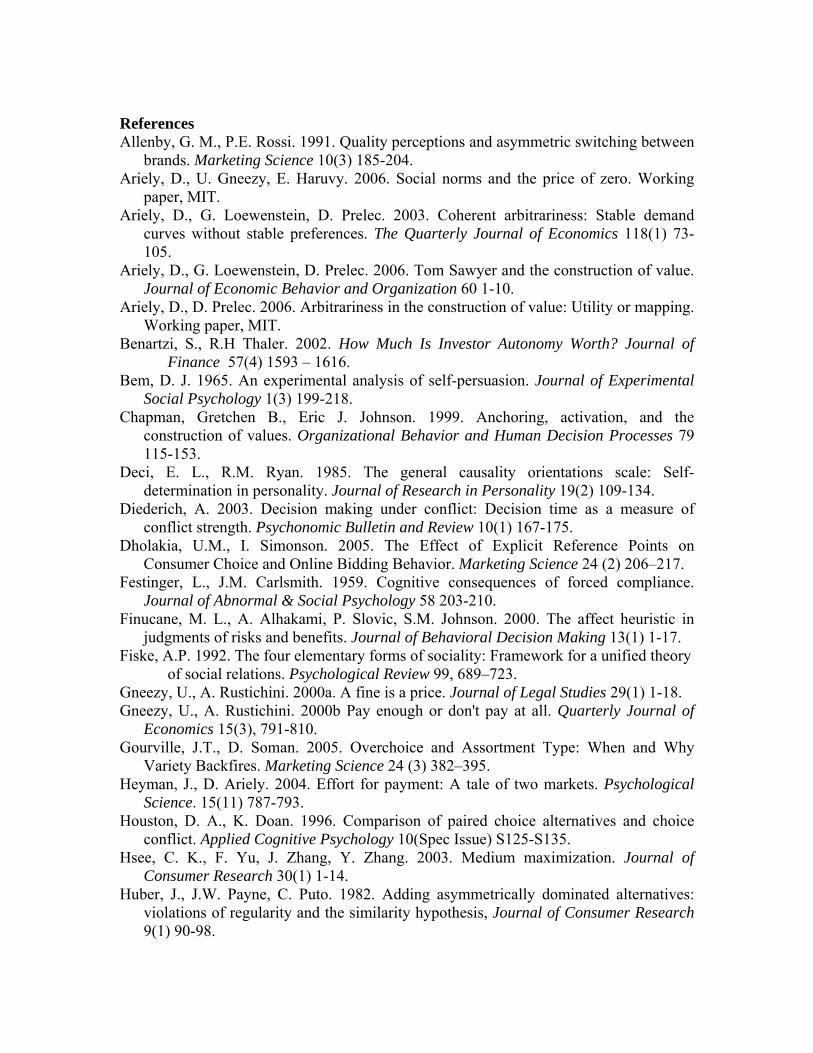
Assume there are multiple consumers with [VX, VY] distributed over R2; the three

sets of inequalities determine three groups of consumers who choose each of the three

options (see Figure 1a).

Now consider a situation in which both prices are reduced by the same amount ε.

The new prices thus are equal to [PX – ε, PY – ε]. How do the demand segments change?

With the new prices, consumers who choose X are those with

VX > PX - ε and VX - PX > VY - PY. (1a)

Consumers choosing Y are those with

VY > PY - ε and VY - PY > VX - PX. (2a)

Finally, consumers choosing N are those with

VX < PX - ε and VY < PY – ε. (3a)

Comparing the two sets of formulas (or inspecting Figure 1b), we note that

consumers who originally choose X keep choosing X, and consumers who originally

choose Y keep choosing Y. Thus, according to this model, there should be no switching

from one product to another. The only two possible changes in demand are that some

consumers who originally buy nothing switch to either X (those with VX - PX > VY - PY

and PX - ε < VX < PX) or Y (those with VY - PY > VX - PX and PY - ε < VY < PY).

9

In short, according to this simple cost–benefit model, when prices decrease by the

same amount, the costs decrease by the same magnitude for both products, whereas their

benefits remain the same, and hence, the net benefits increase by the same amount. In

turn, this model predicts that when the prices of both products drop by the same amount,

both demands increase weakly (see Table 1).

Now consider a special case in which the price reduction, ε, equals the original

smaller price, say PX, so that the prices drop from [PX, PY] to [0, PY - PX]. If zero is just

another price, the preceding predictions remain valid. In our study setting, when prices

decrease from the cost condition to the free condition, the proportion of consumers

choosing each of the two products should increase weakly (see Figure 1c).

Next, consider the zero price model, which assumes that when a product becomes

free, consumers attach a special value to it, that is, their intrinsic valuation of the good

increases by, say, α. Note, the decision to add α to the benefit (intrinsic valuation) of the

free good is rather arbitrary. All the predictions would go through just the same, if we

assume that α is added directly to the net benefit of the free good or subtracted from its

cost, or even added to the costs of all non-free goods (extra pain of paying). We will

discuss the nature of α in more detail after the initial empirical findings are presented.

In this model, and in contrast with the standard model, some consumers switch

from the more expensive good to the cheaper good if their valuations of the products

satisfy the following set of inequalities. The first two inequalities imply the original

choice of Y, and the second two inequalities lead to switching to X when its price is

reduced to zero:

10

VY > PY,

VY - PY > VX - PX,

VX + α > 0, and

VX + α - PX > VY - PY. (4)

That is, as the prices fall from the cost condition to the free condition, the costs

decrease by the same magnitude for both products, the benefit for the now free product

increases more than that for the more expensive product, and the net benefit of the

cheaper product becomes higher. In terms of demand, the zero price model predicts that

as prices are reduced from the cost condition to the free condition, the demand for the

cheaper good increases, and more importantly, the demand for the more expensive good

may decrease as consumers switch from the more expensive product to the cheaper one

(see Table 1, Figure 1d). We refer to the combination of the increase in the proportion of

consumers choosing X and the decrease of those choosing Y when prices fall from [PX,

PY] to [0, PY - PX] as the zero price effect. The prediction regarding the decrease in

demand for the more expensive good represents the one observable difference between

the two models, and thus, in our empirical section, we focus on it.

••• Figure 1 & Table 1•••

4. Testing the Phenomenon

11

In this section, we describe a series of experiments designed to test the validity of

the zero price model and rule out some trivial economic explanations for the changes in

demand that take place as the price of the cheaper good decreases to zero (i.e., from the

cost condition to the free condition).

4.1. Experiment 1: Survey

Method. We asked 60 participants to make a hypothetical choice among a

Hershey’s, a Ferrero Rocher chocolate, and buying nothing (we provided pictures of both

chocolates). Across the three conditions, the prices of the two chocolates decreased by a

constant amount (for a description of all conditions across all the experiments, see the

Appendix). In the cost condition, the prices of Hershey’s and Ferrero were 1¢ and 26¢,

respectively (1&26 condition). In the free condition, both prices were reduced by 1¢ and

therefore were 0¢ and 25¢, respectively (0&25 condition). The third condition (2&27

condition) represents an additional cost condition in which the prices of goods increased

by 1¢ above their prices in the first cost condition. The purpose of the 2&27 condition is

to contrast the effect of a 1¢ price reduction that does not include a reduction to 0

(reduction from 2&27 to 1&26) with a 1¢ price reduction that does (reduction from 1&26

to 0&25).

Results and Discussion. We provide the results in Figure 2. As the prices

decrease from the 1&26 condition to the 0&25 condition, the demand for Hershey’s

increases substantially (t(31) = 3.8, p < 0.001) while, more importantly, the demand for

Ferrero decreases substantially (t(31) = -2.3, p = 0.03), in support of the zero price effect.

The difference in demand between the 1&26 and 2&27 conditions is imperceptible

12

(Hershey’s t(38) = -0.3, p = 0.76; Ferrero t(38) = 0, p = 1), which demonstrates that when

all prices are positive, a 1¢ change in prices does not have a significant effect on demand.

Only when one of the prices becomes zero does the observed perturbation take place.

Thus, we observe (hypothetical) behavior consistent with the zero price model;

participants reacted to the free Hershey’s as if it had additional value.

••• Figure 2 •••

4.2. Experiment 2: Real Purchases

Although the results of Experiment 1 suggest that consumers react to a price

decease to zero differently than they do to other price reductions, their reaction pertains

to a hypothetical situation, which means that it remains an open question whether

consumers will behave in the same way when faced with real transactions. As a

secondary goal, Experiment 2 includes another condition to test the robustness of the zero

price effect. In this condition, the price reduction is much larger for the high-end candy,

which gives participants a greater incentive to make choices opposite to the predictions of

the zero price effect. Furthermore, this unequal price reduction provides a test of the

notion that consumers divide, rather than subtract, costs and benefits (as we discuss

subsequently).

Method. Three hundred ninety-eight subjects took part in the experiment. We use

a Hershey's as the low-value product and a Lindt truffle (hereafter, “Lindt”) as the high-

value product. The experiment includes a free condition (0&14), a cost condition (1&15),

and a second free condition (0&10). In the 0&14 and 0&10 conditions, the price of

13

Hershey's is 0¢, and the price of Lindt is 14¢ and 10¢, respectively. In the 1&15

condition, the price of Hershey's is 1¢, and the price of Lindt is 15¢.

A booth in MIT’s student center contained two cardboard boxes full of chocolates

and a large upright sign that read “one chocolate per person.” Next to each box of

chocolates was a sign lying flat on the table that indicated the price of the chocolate in

that condition. The flat signs could not be read from a distance, and the prices were

visible only to those standing close to the booth. We use the flat signs because we want to

measure the demand distributions, including the number of people who considered the

offer and decided not to partake. By placing the price signs flat next to the chocolates, we

could code each person who looked at the prices but did not stop or purchase and classify

them as “nothing.”

Although field experiments have many advantages, this particular setup suffers a

limitation in that the experimental conditions could not be randomized for each subject;

instead we alternated the price signs (conditions) approximately every 45 minutes. When

replacing the signs, we wanted to reduce the chance that students would notice the

change (which would mix within- and between-subjects designs) and therefore instituted

15-minute breaks between each of the 30-minute experimental sessions.

Results and Discussion. As we show in Figure 3, the results are similar to the

hypothetical choices in Experiment 1. As the prices decrease from the 1&15 condition to

the 0&14 condition, demand for Hershey’s increases substantially (t(263) = 5.6, p <

0.001), while demand for Lindt decreases substantially (t(238) = -3.2, p < 0.01). In

addition, we find no significant difference between the demand for Hershey’s between

the 0&14 and 0&10 conditions (t(263) = 0.5, p = 0.64) and a marginally significant

14

difference in demand for the Lindt between the 0&14 and 0&10 conditions (t(271) = 1.5,

p = 0.13). This marginal difference, however, is in the opposite direction of the expected

effect of a price decrease on demand, which may be related to the higher number of

participants who took nothing in the 0&10 condition. Together, these results show that

the reduction of a price to zero is more powerful than a five-times larger price reduction

that remains within the range of positive prices.

A somewhat surprisingly large proportion of people selected “nothing.” This

observed lack of interest could be due to the way we coded the choice of nothing; some

people who might not even have noticed the offers (and thus effectively were not part of

the experiment) could have been misclassified as buying nothing (instead of being

considered nonparticipants). Another possible contributor to the choice of nothing could

be transaction costs; buying a chocolate or even taking a free chocolate requires attention

and time. Finally, in the experimental setting, the value of chocolate may have been

either not positive or not sufficiently large for our participants.

If we take those whom we coded as nothing out of the analysis, the share of

Hershey’s increases from 27% in the 1&15 condition to 69% in the 0&14 condition and

to 64% in the 0&10 condition. The demand for Lindt shows a complementary pattern:

decreasing from 73% in the 1&15 condition to 31% in the 0&14 condition and 36% in

the 0&10 condition. The difference between the cost and the free conditions is

statistically significant (both ps < 0.001), but the difference between the two free

conditions is insignificant (t(142) = -1.0, p = 0.31).

In summary, the results of Experiment 2 demonstrate that valuations of free goods

increase beyond their cost–benefit differences, as we show with real transactions in a

15

field setting, and even when the price decrease for the high-value product is substantially

larger than that of the low-value product. The observed drop in demand for the high-

value good in such a case (from the 1&15 condition to the 0&10 condition) is

theoretically even more impossible than in the case when prices decrease by the same

amount.

Another advantage of the comparison of the 0&10, 0&14, and 1&15 conditions is

that it sheds some light on the possibility that rather than evaluating options on the basis

of their cost–benefit difference, consumers might consider goods on the basis of the ratio

of benefits to costs (not a normative account). According to this interpretation, the net

value of a free good is very high (strictly speaking, infinite) and therefore leads to the

choice of the free good. However, the results of Experiment 2 weaken the possibility of

this explanation in two ways. First, if our participants followed a strict ratio rule, and if

we assume that everyone has at least an epsilon valuation for Hershey’s, the choice share

of the free chocolate should have been 100%, or at least 100% of those selecting any

chocolate, which is not the case. Second, a less strict version of the ratio rule implies that

the price reduction of the high-end chocolate from 15¢ to 10¢ (a 33% reduction) should

have had a much larger effect on its share compared with the price reduction from 15¢ to

14¢ (a 7% reduction). This prediction does not bear out; there is no real difference in the

changes in demand when the prices fall from 1&15 to 0&14 on the one hand and to 0&10

on the other hand.

••• Figure 3 •••

16

4.3. Experiment 3: Cafeteria.

We acknowledge a possible shortcoming of Experiment 2; namely, the difference

between conditions may not be confined to prices, such that the size of the transaction

costs associated with the three options differs among conditions. Taking a free Hershey’s

or buying nothing means not only a zero monetary price but also no associate hassle of

looking for change in a pocket or backpack. If transaction cost is a consideration in our

setting, it could lead to a choice pattern that favors Hershey’s when its cost is zero (in the

0&14 and 0&10 conditions), but not when both options involve a positive cost and hence

a larger transaction cost (the 1&15 condition). We derive an initial indication that

transaction cost is not the driver of the effect from the results pertaining to the

hypothetical choices in Experiment 1. Because Experiment 1 does not involve real

transactions, it does not involve any transaction costs, which implies the results will

survive a situation without transaction costs. However, though these results are

indicative, when respondents made their hypothetical choices, they might have

considered transaction costs that would have been present if the choice they were facing

had been real. Because the results of Experiment 1 cannot be interpreted conclusively and

because transaction costs could be an important alternative explanation, we conduct

Experiment 3, designed explicitly to control for possible differences in transaction costs.

In this experiment, we hold the physical transaction costs constant for the three choices

(high- and low-value chocolates and no purchase) and between the cost and free

conditions.

Method. We carried out this experiment as part of a regular promotion at one of

MIT’s cafeterias, using customers who were already buying products at the cafeteria and

17

adding the cost of the chocolate to their bill as if it were any other purchase. By adding

the cost to an existing purchase, we create a situation in which the chocolate purchase

does not add anything to the transaction costs in terms of taking out one’s wallet, looking

for money, paying, and so forth.

The procedure of the experiment is generally similar to that used in Experiment 2:

a box with two compartments, one containing Hershey's and the other containing Lindt,

appeared next to the cashier. A large sign read “one chocolate per person,” and we posted

the price of each chocolate next to each compartment (varying across conditions).

Customers who wanted one of the chocolates had its cost added to their bill. Thus, the

transaction costs in terms of payment remained the same whether a customer purchased a

chocolate, got a chocolate for free, or purchased nothing, because he or she still had to

pay for the main purchase.

We manipulated the prices at two levels: 1¢ for Hershey’s and 14¢ for Lindt in

the cost condition, and 0¢ and 13¢, respectively, in the free condition. We switched the

price signs (conditions) approximately every 40 minutes, with a 10-minute break between

the experimental sessions. In this setting, it was difficult to separate customers who

decided not to participate from those who did not notice the offer; therefore, all

customers who passed by the cashier and did not select any of our chocolates were coded

as “nothing.” In total, 232 customers took part in this experiment.

Results and Discussion. As we show in Figure 4, in the condition in which

Hershey’s is free, the demand for Hershey’s increases substantially (t(189) = 4.7, p <

0.001), while the demand for Lindt decreases substantially (t(206) = -3.2, p = 0.001). If

we remove those whom we code as nothing from the analysis, the share of Hershey’s

18

increases from 21% in the 1&14 condition to 71% in the 0&13 condition, whereas the

share of Lindt decreases from 79% in the 1&14 condition to 29% in the 0&13 condition

(t(92) = 5.6, p < 0.0001).

Thus, the zero price effect is not eliminated when transaction costs are the same

for all options and in both conditions, which provides strong evidence that the zero price

effect is not produced solely by a difference in transaction costs.

••• Figure 4 •••

4.4. Summary of the Initial Experiments

These initial experiments contrast the choices respondents make when the prices

for both options are positive relative to a case in which both options are discounted by the

same amount, such that the cheaper option becomes free. This methodology enables us to

examine the reaction to free offers and indicates both an increase in demand for the

cheaper product and a decrease in demand for the more expensive product, an effect we

term the zero price effect.

Experiment 1 demonstrates that a 1¢ difference in price has an enormous

influence on demands if it represents a difference between a positive and zero prices but

not when it is a difference between two positive prices. Participants reacted as if a free

Hershey’s had more intrinsic value than a positively priced Hershey’s. Experiment 2

validates this finding with real choices and argues against the ratio explanation. Finally,

Experiment 3 demonstrates that the zero price effect is not driven by transaction costs.

19

Thus, we show that for prices, as for many other domains, zero is treated qualitatively

differently from other numbers.

When we consider how zero might differ from other numbers, we posit two

general answers: The first relies on the proposed model and assumes a unique benefit of

the price of zero, which leads to a demand discontinuity at zero. A second approach is to

model this process with a concave utility of money. In such a model, instead of

evaluating options by V - P (i.e., value minus price), consumers evaluate them by V -

v(P), where v is the prospect theory value function (Kahneman and Tversky 1979). To

illustrate this point, consider the choices from Experiment 3: If the net benefit of a

chocolate is defined by V - v(P), participants could switch from Lindt to Hershey’s

because v(14¢) - v(13¢) < v(1¢). The utility of money is likely to be generally concave

(Kahenman and Tversky 1979), so the question for our purposes is not whether it is

concave but rather whether concavity may account for our findings. Moreover, the

discontinuity in zero that we propose represents a special case of concavity; a function

that is zero at zero and then “jumps” and is upward sloping and linear (or concave) is by

definition concave. Our question therefore pertains to whether the effect of the price of

zero is captured better by a continuous or discontinuous concave utility of money.

To examine the possibility that continuous concavity could be sufficient to

account for the results, we consider the contrast between the two price reductions in

Experiment 1: from 2&27 to 1&26 and from 1&26 to 0&25. A model claiming that a

continuous concave utility function of money can account for the results would assume

that consumers evaluate the options by V - v(P), that v(26¢) - v(25¢) < v(1¢), and that this

difference is sufficient to explain the large zero price effect documented in Experiment 1.

20

However, this model would have to assume also that v(27¢) - v(26¢) < v(2¢) - v(1¢), and

thus, we should expect an increase in demand for Hershey’s and a decrease in demand for

Ferrero in the 1&26 versus the 2&27 condition. Such demand changes should be smaller

in magnitude than those between 1&26 and 0&25, but they would occur in the same

direction. However, as we show in Figure 2, the results do not indicate anything of the

kind. Although concavity is present in the utility of money, the type of concavity in our

setting is more likely to exist because of a discontinuity at zero rather than continuous

concavity alone (we provide further support for the discontinuous nature of the zero price

in the Amazon gift certificates experiment and a flat screen televisions experiment

described later).

5. Why Is Zero Price Special?

In the first part of this article, we demonstrate that zero price has a special role in

consumers’ cost–benefit analysis. In this section, we take another step toward exploring

the psychology behind the zero price effect. In particular, we consider three possible

explanations, which we label “social norms,” “mapping difficulty,” and “affect.” On the

basis of prior research and an additional study, we argue that the social norms

explanation, though applicable in some cases, cannot account fully for the zero price

effect, so we focus on distinguishing between the mapping difficulty and affect accounts.

Overall, the results support the role of affect as a main cause for the effect of zero.

5.1. Social Norms

21

A possible psychological mechanism that could underlie the zero price effect

deals with the norms that might accompany free products. Costly options invoke market

exchange norms, whereas free products invoke norms of social exchange (Fiske 1992,

McGraw, Tetlock, and Kristel 2003, McGraw and Tetlock 2005). Thus, evoked social

norms may create higher value for the product in question. Heyman and Ariely (2004)

offer one example in which they demonstrate that people are likely to exert higher effort

under a social contract (no monetary amounts) than when small or medium monetary

amounts are mentioned. Another example of the relationship between social and

exchange norms appears in Ariely, Gneezy, and Haruvy’s (2006) research, in which they

examine the behavior of persons faced with a large box of candies and an offer to receive

the candy either for free or for a nominal price (1¢ or 5¢). Not surprisingly, when the cost

is zero, many more students take candy than when the price is positive. More interesting,

when the price is zero, the majority of the students take one and only one candy, while

those who pay to take candy take a much larger amount (effectively creating lower

demand as prices decrease).

Together, these results suggest that social norms are more likely to emerge when

price is not a part of the exchange, which could increase the valuation for a good and, in

our experiments, increase the market share of the free chocolate. However, another

condition in Heyman and Ariely’s (2004) experiments suggests that the effect of social

norms might not apply to our settings. When the elements of both social exchanges (e.g.,

a gift) and monetary exchanges occur (e.g., “Here is a 50¢ candy bar”), the results are

very similar to those of a monetary exchange and different from those of a social

exchange. Relating these findings to our setting suggests that it is highly unlikely

22

participants apply social exchange norms to one option in the choice set (free option) and

monetary exchange norms to the other (cost option). Instead, participants probably apply

the same set of norms to all choices in the set and thereby eliminate the effect of social

exchange norms.

To test the ability of social exchange norms to account for the zero price effect

further, we create an additional condition that enables us to disassociate the free cost

from the social norms invoked by the lack of cost. That is, we offer the low-value

chocolate for a small negative price (-1¢), which creates a transaction with no downside

(no financial cost) but still mentions money and thus presumably does not invoke social

exchange norms. To the extent that the zero price effect is due to the social nature of

nonmonetary exchanges, a negative price, which has no social aspect, should not induce

an increase in the intrinsic valuation of the products in the same way zero price does.

However, if the zero price effect is not due to social exchange norms, demand in this

condition should be very similar to that in the free condition.

Three hundred forty-two subjects took part in this experiment, which replicates

the 1&14 and 0&13 conditions of Experiment 2 with the addition of a -1&12 condition,

in which the price of Hershey's is -1¢ (participants received Hershey’s plus a penny) and

the price of Lindt is 12¢. The demands in the 1&14 and 0&13 conditions replicate our

previous findings: Compared with the 1&14 condition, the demand for Hershey’s in the

0&13 condition increases substantially from 15% to 34% (t(193) = 3.4, p < 0.001), and

the demand for Lindt decreases substantially from 38% to 16% (t(212) = -3.8, p < 0.001).

Of greater significance, we find that when prices drop from 0&13 to -1&12, the demand

for Lindt remains 16% (t(220) = 0.04, p = 0.97), but the demand for Hershey’s increases

23

from 34% to 50% (t(212) = -3.8, p < 0.001). Thus, in contrast with the social exchange

norms explanation, the zero price effect remains even when we mention money for both

options in the choice set. These results also suggest that a change in the cost–benefit

analysis likely causes the shift in evaluations for the free (or small negative cost) product.

5.2. Mapping Difficulty

A second possible psychological mechanism that might explain the overemphasis

on free options comes from the findings of Ariely, Loewenstein, and Prelec (2003, 2006),

Hsee et al. (2003), and Nunes and Park (2003), which demonstrate that people have

difficulty mapping the utility they expect to receive from hedonic consumption into

monetary terms. In one set of studies that illustrates this mapping difficulty, Ariely,

Lowenstein, and Prelec (2003) demonstrate that maximum willingness to pay (elicited by

an incentive-compatible procedure) is susceptible to anchoring with an obviously

irrelevant number—the last two digits of a social security number (Tversky and

Kahneman 1974; Chapman and Johnson 1999). For example, students whose last two

digits of their social security numbers were in the bottom 20% of a distribution priced a

bottle of 1998 Cotes du Rhone wine at $8.64 on average, whereas those whose last two

digits were in the top 20% priced the same bottle at $27.91 (see also Simonsohn and

Lowenstein 2006). These results suggest it is difficult for decision makers to use their

internal evaluations for products, so they resort to the use of external cues to come up

with their valuations.

Mapping difficulty could play a role in our setting as well. To the extent that

evaluating the utility of a piece of chocolate in monetary terms is difficult, consumers

24

might resort to a strategy that assures them of at least some positive surplus. Specifically,

receiving a piece of the lower-value chocolate for free must involve positive net gain, but

paying for a piece of the higher-value chocolate may or may not. To illustrate, imagine a

situation in which a consumer’s valuation for the lower-value chocolate is somewhere

between 1¢ and 5¢ and his or her valuation for the higher-value chocolate is between 10¢

and 20¢. If this consumer were faced with the 1&14 condition, it would be unclear which

of the options would give him or her a net benefit or the higher net benefit. However, the

same consumer facing a 0&13 condition easily recognizes that the free option definitely

provides a net benefit, so the consumer chooses that option. Thus, the zero price effect

might be attributed, according to this perspective, to the uncertainty surrounding the

overall benefit associated with costly options and the contrasting certainty about overall

benefits associated with free options.

5.3. Affect

A third possible psychological mechanism that might account for the zero price

effect pertains to affect, such that options with no downside (no cost) invoke a more

positive affective response; to the extent that consumers use this affective reaction as a

decision-making cue, they opt for the free option (Finucane et al. 2000, Slovic et al.

2002a, Gourville, and Soman 2005). We test this prediction directly with Experiment 5.

The affective perspective also suggests the circumstances in which the zero price effect

should be eliminated: If the cause of the zero price effect is a reliance on an initial (overly

positive) affective evaluation, making a non-affective, more cognitive evaluation

accessible might diminish the zero price effect.

25

To test which of these two psychological mechanisms (mapping difficulty, affect)

is the more likely driver of the zero price effect, we conduct three more experiments. In

Experiment 4, we attempt to reduce or eliminate the mapping difficulty to observe

whether that diminishes or eliminates the zero price effect. In Experiment 5, we test the

first proposition of the affective account, namely, that free offers elicit higher positive

affect. In Experiment 6, we test whether forcing people to evaluate the options

cognitively, and thereby making these evaluations available and accessible, eliminates the

zero price effect.

5.4. Experiment 4: Halloween

Experiment 4 aims to test whether mapping difficulty could be driving the zero

price effect. Therefore, we reduce mapping difficulty by making both sides of the

transactions (i.e., that which participants stand to gain and that which they relinquish)

commensurable. We predict that to the extent that mapping difficulty is the cause of the

zero price effect, it will diminish when the two sides of the transaction match. We also

predict that this type of manipulation will have no bearing if affect is the cause of the

zero price effect.

Method. To reduce mapping difficulty, participants were able to exchange

chocolate for chocolate rather than for money. Specifically, on Halloween, 34 trick-or-

treaters at an authors’ house were exposed to a new Halloween tradition. As soon as the

children knocked on the door, they received three Hershey's (each weighing about 0.16

oz.) and were asked to hold the Hershey’s they had just received in their open hand in

front of them. Next, each child was offered a choice between a small (1 oz.) and a large

26

(2 oz.) Snickers bar. In the free (0&1) condition, they could simply get the small Snickers

bar or exchange one of their Hershey's for the large Snickers bar. In the cost (1&2)

condition, the children could exchange one of their Hershey's for the small Snickers bar

or exchange two for the large Snickers bar. They also could choose not to make any

exchanges.

Results and Discussion. As we show in Figure 5, the zero price effect remains

strong even when the trade-offs involve commensurate products and exchange media

(“money”). In the 0&1 condition, in which the small Snickers bar is free, demand for it

increases substantially (relative to the cost condition), whereas demand for the large

Snickers bar decreases substantially (t(31) = 4.9, p < 0.001). A follow-up experiment

with adults, conducted at the MIT Student Center in a setting similar to Experiment 2,

includes the 0&4 and 1&5 conditions for exchanges involving Hershey’s for small and

large Snickers, respectively. The results replicate the pattern of results of the Halloween

experiment.

These results generalize our previous findings in five ways. First, they

demonstrate that the attractiveness of zero cost is not limited to monetary transactions;

there seems to be a general increase in attractiveness of those options that do not require

giving up anything. Second, the results hold when the goods and exchange currency are

commensurate—in this case, chocolate-based candy (for other results regarding

commensurability, see Ariely, Loewenstein, and Prelec 2003; Hsee et al., 2003; Nunes

and Park, 2003). Third, though a 1¢ price is not very common in the marketplace, the

choice and trading of candy is more common (particularly in the context of Halloween),

which adds ecological validity to our finding. Fourth, the results provide further support

27

that the physical hassle involved in transactions cannot account for the results. Fifth, this

effect holds for adults as well as for children.

••• Figure 5 •••

As a further test of the mapping account for the effect of zero prices, we conduct

another experiment in which both the products and the method of payment were money.

The two products participants could choose from were $10 and $20 Amazon gift

certificates (or “neither”). The prices for the gift certificates were varied at three levels:

$5 and $12, $1 and $8, and $0 and $7, respectively, with the $20 certificate always

costing $7 more than the $10 certificate. As the reader may guess, we find no differences

in demand patterns between the 5&12 and the 1&8 conditions (t(65) = 0.53, p = 0.6), but

demand for the $10 certificate rockets in the 0&7 condition (t(65)= 6.9, p < 0.001) while

demand for the $20 certificate falls to zero (see Figure 6). Thus, the experiment further

invalidated mapping difficulty as a source of the zero price effect; the effect survived a

situation in which the product sold and the medium were both monetary.3

This lack of difference in demand between the 5&12 and 1&8 conditions,

together with the large shift in demand in the 0&7 condition, also argues against a ratio

account. The ratios of the costs are much more favorable toward the $10 Amazon gift

certificate in the 1&8 condition compared with the 5&12 condition (by approximately 3.3

times), so if participants actually used the ratio rule, we would have observed a large

3 We use gift certificates in this experiment to test whether mapping difficulty can account for the zero price effect, and they are definitely closer to money relative to chocolates. Of course, Amazon gift certificates are not exactly money, for example, they are not entirely fungible (Waldfogel 1993). It seems likely that if we were selling money for money, everybody would prefer to trade $7 for $20 to trading nothing for $10.

28

increase in demand for the $10 Amazon gift certificate in the 1&8 condition, which we

did not.

The availability of multiple conditions with both positive prices in this experiment

also helps us examine whether gradual price reduction to zero creates a continuous or

discontinuous changes in demand and hence whether v(P) is continuous at zero.

Continuous change would most likely result in at least a slight difference between the

5&12 and 1&8 conditions, and a (potentially larger) difference between the 1&8 and 0&7

conditions. The observed lack of the former difference suggests that discontinuity of v(P)

at zero might be a better account for our data.

••• Figure 6 •••

In summary, the main reason for our Halloween and Amazon gift certificate

experiments was to test whether the difficulty of mapping money onto experiences could

be the cause of the zero price effect. We first replaced money as the exchange medium

with chocolates, which presumably can be mapped more naturally onto other chocolates.

We then replaced the product and the exchange medium with money. The results

demonstrate that the zero price effect is not limited to goods-for-money exchanges and

that it is unlikely to be explained fully by mapping difficulties.

5.6. Experiment 5: Smilies

The affect account has two basic components. The first is that free offers evoke

higher positive affect, and the second is that people use this affect as an input for their

29

decision-making process. In Experiment 5, we examine the first component: People

experience more positive affect when facing a free offer compared with other offers.

Method. We asked 243 participants to evaluate how attractive they found an offer

of a chocolate at a certain price. We manipulated the offer on four levels among

participants: Hershey’s for free (H0), Hershey’s for 1¢ (H1), Lindt for 13¢ (L13), and

Lindt for 14¢ (L14). Participants received a questionnaire with the details of the offer and

a picture of the chocolate. At the bottom of the page, schematic pictures of five faces

(“smilies”) with different expressions appeared, varying from unhappy to very happy.

Participants were asked to indicate their feelings toward the offer by circling one of the

faces. If participants’ attitude toward the offers reflected the offers’ net benefits, the

attitudes toward L14 and H1 should be slightly lower than those toward L13 and H0,

respectively; and the difference between the attitudes toward L13 and L14 should be

similar to the difference between H0 and H1. The affect argument, however, suggests that

the attitude toward H0 should be much higher than that toward any other offer.

Results and Discussion. We depict the results in Figure 7. In line with the affect

hypothesis, attitude toward the H0 offer is significantly higher than attitude toward any

other offer (t(113) = 7.0, p < 0.001). Furthermore, we find no difference among the

attitudes toward the other three offers (F(2, 178) = 0.35, p = 0.7). In support of the affect

idea, the free good elicits more positive affect than standard cost–benefit analysis

predicts.

Why does a free Hershey’s elicit such higher positive affect relative to a 13¢

Lindt? Ex ante, it is possible that a Lindt at 13¢ provides a much better deal than a

Hershey’s at any price. In fact, when people carefully consider the pros and cons of these

30

offers, they much more often come to conclusion that the value of 13¢ Lindt is higher

than that of a free Hershey’s (see Experiment 6). But, as the results of Experiment 5

demonstrate, it is also clear that the free Hershey’s creates much higher affective

reaction. One reason for this could be that that the decision to take a chocolate for free is

a much simpler decision, and that simplicity could be the driver of higher affect (Tversky

and Shafir 1992, Luce 1998, Iyengar and Lepper 2000, Benartzi and Thaler 2002,

Schwarz 2002, Diederich 2003, Gourville and Soman 2005). In particular, a free

Hershey’s involves benefits and no costs, while a Lindt for any positive price involves

both benefits and costs – it is possible that options that have only benefits create more

positive affect compared with options that involve both benefits and cots. Alternatively,

much like the disutility of paying while consuming (paying for a vacation while

experiencing it: Prelec and Loewenstein 1998), it is possible that options that involve

both benefits and cots create a negative impact on affect due to the simultaneity of these

two components, while options that have only benefits do not include this “penalty.”

••• Figure 7 •••

5.7. Experiment 6: Forced Analysis

In response to the high affective reaction to the free option in Experiment 5, we

test whether consumers use this increased affect as a cue for their decisions, which in turn

causes the zero price effect. In Experiment 6, we force participants to engage in a

cognitive and deliberate evaluation of the alternatives before they choose and thereby we

make non-affective, more cognitive evaluations available and accessible to participants.

31

We assume that in these conditions, participants are more likely to base their evaluations

on cognitively available inputs and therefore place a lower weight on the affective

evaluations. To the extent that the cause of the zero price effect is the affective

component, such reliance on cognitive inputs should reduce the zero price effect.

Method. Two hundred students filled out a survey in which they made a

hypothetical choice among three options. We also asked half the subjects to answer two

questions before making the choice. The design was a 2 (chocolates’ prices: 1&14 vs.

0&13) × 2 (survey type: neutral vs. forced analysis) between-subjects design.

The survey in the [1&14, neutral] condition asked participants to imagine that

there is a chocolate promotion at the checkout counter of their supermarket and that they

could either buy one Hershey’s kiss for 1¢ or one Lindt truffle for 14¢. Participants

indicated their preferred option (a Hershey’s for 1¢, a Lindt for 14¢, or neither). The

[0&13, neutral] condition mirrored the 1&14 condition, except that Hershey’s and Lindt

were offered for free and 13¢, respectively.

In the forced analysis conditions, after reading the introduction but before being

asked for their hypothetical choice, participants were asked the following two questions:

“On a scale from 1 (not at all) to 7 (much more) how much more do you like the Lindt

truffles in comparison with Hershey’s kisses?” and “On a scale from 1 (not at all) to 7

(much more) how much more would you hate paying 14¢ (13¢) in comparison with

paying 1¢ (nothing)?” Participants circled a number from 1 to 7, anchored at 1 (not at

all), 4 (about the same), and 7 (much more). After answering these questions, participants

made their hypothetical choice among the three options.

32

Results and Discussion. We ran two logit regressions with the proportions of

subjects buying Hershey’s and Lindt as the dependent variables and the answers to the

two questions as independent variables (forced analysis conditions only). Unsurprisingly,

preferring Lindt to Hershey’s is related negatively to choosing Hershey’s (z = 3.1, p <

0.01) and positively to choosing Lindt (z = 3.0, p < 0.01). Disliking paying more is

related positively to choosing Hershey’s (z = 3.2, p = 0.001) and negatively to choosing

Lindt (z = 3.1, p < 0.01). Thus, participants’ answers to the questions fall in line with

their choices.

Next, we performed two ANOVAs with the proportions of subjects choosing

Hershey’s and Lindt as the dependent measures and the chocolates’ prices, survey type,

and the interaction term as independent variables. The ANOVAs reveal significant main

effects of chocolates’ prices (Hershey’s F(1, 196) = 9.7, p < 0.01; Lindt F(1, 196) = 8.7, p

< 0.01), no main effects of survey type (Hershey’s F(1, 196) = 2.0, p = 0.2; Lindt F(1,

196) = 1.6, p = 0.2), and, most importantly, a significant interaction effect for the two

factors (Hershey’s F(1, 196) = 4.5, p = 0.03; Lindt F(1, 196) = 5.1, p = 0.02).

As we demonstrate in Figure 8, the zero price effect is replicated in the neutral

conditions (Hershey’s t(97) = 3.7, p < 0.001; Lindt t(97) = -3.7, p < 0.001) but not in the

conditions in which subjects compare their quality and price options before choosing. In

the forced analysis conditions, the direction of the effect remains the same, but the

magnitude is much smaller and statistically insignificant (Hershey’s t(99) = 0.7, p = 0.5;

Lindt t(99) = -0.6, p = 0.6). These results support the basic affect mechanism we propose,

according to which the affect invoked by the free option drives the zero price effect, but

33

when people have access to available cognitive inputs, they base their decisions on those,

and the benefit of zero largely dissipates.

Another potential interpretation of these results is that in three of our four

conditions, subjects act “rationally”—the two forced analysis conditions and the [1&14,

neutral] condition. In the [0&13, neutral] condition, however, they act on the basis of the

affect evoked by the zero price. In support of this idea, we find no significant difference

among subjects’ choices in the three rational conditions (Hershey’s F(2, 147) = 0.7, p =

0.5; Lindt F(2, 147) = 0.7, p = 0.5), whereas the [0&13, neutral] condition differs

significantly from them (Hershey’s t(83) = 3.8, p < 0.001; Lindt t(83) = 0.3.7, p < 0.001).

••• Figure 8 •••

6. General Discussion

We start with two models, one that treats zero as just another price and one that

assumes free options are evaluated more positively. We propose a method to distinguish

these two approaches and demonstrate in three experiments that the latter model is better

able to account for our findings. Experiment 1 provides the initial evidence of the zero

price model, and Experiment 2 supports the effect with a real buying scenario and

clarifies that the effect could not be due to decision making based on cost–benefit ratios.

Experiment 3 shows that the effect also could not be due to physical transaction costs.

After demonstrating the unique properties of zero price, we attempt to examine

the psychological causes for this effect and propose three possible mechanisms: social

norms, mapping difficulty, and affect. We discard the social norms explanation on the

34

basis of findings (Heyman and Ariely 2004) that the mention of price invokes market-

based transaction norms, which makes it unlikely that our scenario invokes social norms.

We further discredit the ability of this account to explain our findings using negative

prices that involve no cost but invoke prices. We then carry out three experiments to

explore which of the other two possible explanations is valid. Experiment 4 weights in

against the difficulty of mapping explanation, and Experiments 5 and 6 provide support

for the affective evaluation hypothesis.

In general, this research joins a larger collection of evidence that shows zero is a

unique number, reward, price, and probability. Although our results suggest that the zero

price effect might be accounted for better by affective evaluations than by social norms or

mapping difficulty, zero and the price of zero remain a complex and rich domain, and all

of these forces may come into play in different situations. In addition, other effects of

zero might include inferences about quality, changes in signaling to the self and others,

an effect on barriers for trial, and its ability to create habits. Therefore, much additional

work is needed to understand the complexities of zero prices in the marketplace.

6.1. Alternative Explanations and Boundary Conditions

One of the limitations of our experimental conditions is that they are restricted to

relatively cheap products and relatively unimportant decisions. Given this limitation, it

remains an open question whether the zero price effect occurs when the decisions involve

higher stakes. To answer this question, at least partially, we distributed a survey in which

participants responded to one of four hypothetical scenarios regarding purchasing an

LCD flat-panel television. In these scenarios, participants were entitled to a large

35

discount and had narrowed down their options to two: a cheaper 17” Philips and a more

expensive 32” Sharp. The four conditions varied in terms of prices, such that the Sharp

was always $599 more expensive than the Philips, and the prices of both sets decreased

by approximately $100 across conditions. From most expensive to least expensive, the

conditions were 299&898, 199&798, 99&698, and 0&598. Comparing demand across

these conditions, we find that the results (n = 120) generally resemble our previous

findings. Demand for the smaller, cheaper television is 40% in the 299&898 condition,

40% in the 199&798 condition, 43% in the 99&698 condition, and 83% in the 0&698

condition. Concurrently, demand for the larger, more expensive television is 40% in the

299&898 condition, 33% in the 199&798 condition, 43% in the 99&698 condition, and

17% in the 0&698 condition. Overall, these results show that a shift in demand is

apparent only when the price is reduced to zero (F(3,98) = 3.24, p < 0.05); otherwise, the

effects of price reductions do not have a significant influence on the relative demand for

the two televisions (F(2,69) = 0.06, p = 0.94), providing additional evidence against the

continuous concavity argument.

Although these results suggest that the effect of the price of zero is not limited to

small prices and meaningless decisions, some thought experiments also imply it might

not be as simple with large, consequential decisions. For example, if we replace

Hershey’s and Lindt with Honda and Audi and change the prices from $28,000 and

$20,000 to either $8,100 and $100 or $8,000 and $0, respectively, we suspect that

relatively small prices such as $100 might be perceived within a just noticeable

difference zone of zero, such that the effect of zero might be stretched to accommodate

36

this price. Thus, the question of which prices people perceive as zero might not be

simple, because it likely relates to the context of the decision and the original prices.

Another possible limitation of our setup is that our positive prices could seem

suspicious. People in general are not accustomed to prices of 1¢, 13¢, or 14¢, whereas

free samples often are a part of a promotion, which would make people more accustomed

to them. We selected such odd prices because we wanted to have a very small discount

(1¢), while avoiding alternative accounts related to accumulation and disposal of small

change across the different conditions (assuming that people are aversed to having many

small coins fill their pockets). At the same time, these odd prices could have evoked

suspicion, and our participants might have been making negative quality inferences about

the cheap chocolates (the ones with odd prices) but not about the free chocolates. Three

of the experiments cast doubt on this type of argument: In the Amazon gift certificates

experiment the perceived quality of the gift certificates was unlikely to be influenced by

price; in the Halloween experiment, all trade-offs were equally strange; and in the

televisions experiment we gave an explicit explanation for the strange prices: “Luckily

for you, you won a lottery that the store had conducted for its best customers. As a result,

you are entitled to a huge discount on any product in the store.”

To test this “negative inference from odd prices” alternative account more

directly, we conducted two additional experiments. In one experiment we asked

participants to make hypothetical choice among Hershey’s, Lindt, and nothing but this

time used prices that were less suspicious (0&15 and 10&25). The results replicate our

previous findings, with demand for Hershey’s increasing from 8% in the 10&25

condition to 65% in the 0&15 condition (t(51) = 6.0, p < 0.0001) and demand for Lindt

37

decreasing from 45% in the 10&25 condition to 6% in the 0&15 condition (t(54) = 3.8, p

< 0.001 ). In the second experiment we described in detail the setup of the Cafeteria

Experiment (Experiment 3), and measured the inferences participants made about the

products. Half of the participants read the description of the 0&13 condition, and the

other half read the description of the 1&14 condition. After reading and viewing the

verbal and graphical descriptions, the participants were asked to describe their reaction to

the promotion in an open-ended manner, followed by seven questions in which they were

asked to rate the promotion on oddity and the chocolates on perceived quality, taste, and

expiration date (relative to the same brand chocolates from a supermarket). The written

protocols reveal that though participants mention that the promotion is odd (in particular,

because of the “One chocolate per person” sign), or that the prices are odd; none of the

participant spontaneously mentions the quality of the chocolates or makes any price-

quality inferences. In addition, the rating in the seven questions reveal no differences in

promotion oddity or inferences about chocolate quality (or taste, or expiration date)

between the conditions. In general, even though the promotion is seen as somewhat odd

by the participants, they do not make any differential inferences for the condition with

low positive prices vs. the zero price condition.

Even though the zero price effect does not appear to be driven by the oddities of

the prices we used, we do not assume that the price of zero effect will never interact with

processes relating to consumers’ inferences about quality. In many market situations,

consumers might infer the expected quality of the product on the basis of such small

prices, the price of zero itself, or the availability of free giveaway promotions (Simonson,

Carmon, and O’Curry 1994).

38

Finally, the asymmetric dominance effect could offer another possible explanation

for our findings (Huber, Payne, and Puto 1982). In our free conditions, the cheaper

product always weakly dominates the buying nothing alternative, because they share the

same cost (zero) and clearly differ in their benefits. In the cost conditions, no such

asymmetric dominance relationship exists. If the zero price effect in our experiments is

driven by the asymmetric dominance effect, the relationship between the option to buy

nothing and the cheaper chocolate (whether dominant or not) serves as the basic cause for

the effect. Moreover, if we exclude the option not to buy anything, the asymmetric

dominance relationship no longer exists, and any effect due to it should be eliminated. To

test this asymmetric dominance explanation, we conducted a survey (n = 136) in which

we excluded the buy-nothing option (which we could only do in a hypothetical choice

study) and contrasted the zero price effect with the case in which participants had the

buy-nothing option. The results replicate our standard findings: Free Hershey’s

experiences a demand boost (from 28% to 92%) while Lindt suffers a demand decrease

(from 72% to 8%, t(50) = 6.8, p <0.0001), even in the absence of a dominated

alternative. Moreover, these changes in demand are basically identical to the case in

which the option to select nothing appears. Although the asymmetric dominance

therefore is an unlikely explanation for our findings, there are other context effects

ranging from product assortments to reference points in online auctions (e.g. Dholakia,

and Simonson 2005, Leclerc, Hsee, and Nunes 2005) that could relate to these findings.

Thus, we note that the more general questions of what context effects might be involved

and influence prices of zero remain open and interesting.

39

6.2. Managerial Implications

The most straightforward managerial implication of our findings pertains to the

increased valuations for options priced at zero. When considering promotions at a low

price, companies should experiment with further discounts to zero, which likely will have

a surprisingly larger effect on demand. At least one piece of anecdotal evidence supports

this claim. When Amazon introduced free shipping in some European countries, the price

in France mistakenly was reduced not to zero but to one French franc, a negligible

positive price (about 10¢). However, whereas the number of orders increased

dramatically in the countries with free shipping, not much change occurred in France.

This example also suggests that when trying to use bundling with a cheap good in order

to bring up the sales of another good, it might be wise to go all the way down with the

cheap good and offer it for free.

Our findings show that people tend to ignore the opportunity cost associated with

getting things for free (in our experiments the cost is giving up the truffle). Similarly,

people seem to widely ignore the opportunity cost (and other costs) associated with

getting free content online. These costs include the attention cost (being exposed to

unwanted advertising) as well as the search costs – the time spent on finding a song or an

article free of charge, rather than paying for it. As the business model of content

providers slowly changes from free content and revenue generating advertisement to paid

content, they should be wary of the fact that people seem more attracted to offers that

involve zero monetary cost and hidden opportunity cost relative to offers that involve

monetary costs.

40

41

Our findings also suggest that the advantage of the buy-one-get-one-free (BOGO)

promotions over all-at-half-price promotions might go beyond the standard price

discrimination argument. The sales might go further up in the BOGO case, because of

the extra positive affect that “free” creates. Of course, further research would be needed

to determine whether “free” actually creates more affect than “half-price.”

Another possible implication of the effect of zero might be in the domain of food

intake. When designing food and drink products, companies can decide whether to create

low caloric (or fat or carbohydrate) content or reduce these numbers further to zero.

Assuming that the effect of zero generalizes to other domains, investing further effort to

create a product with zero grams of fat might have a very positive influence on demand.

Decisions about zero might be more complex but also more relevant in domains

in which multiple dimensions can occur separately but be consumed together. In the

domain of prices, some examples might include cars or computers, for which price is

composed of a sum of multiple components, some of which might be set at a standard

price and some at zero. In the food domain, these components might be calories, grams of

fat, carbohydrates, amount of lead, and so forth, such that some offer a standard amount

and some are set to zero. To the extent that the effect of zero holds for individual

dimensions that are a part of a complete product, it might be beneficial to consider it at

such levels as well.

Appendix: The different types of goods, prices and dependent measures across experiments and conditions.

Experiment Dependent

Variable Condition Low-Value Good High-Value Good

0&25 Hershey’s kiss for 0¢ Ferrero Rocher for 25¢

1&26 Hershey’s kiss for 1¢ Ferrero Rocher for 26¢ Experiment 1 Hypothetical

choice 2&27 Hershey’s kiss for 2¢ Ferrero Rocher for 27¢

0&14 Hershey’s kiss for 0¢ Lindt Truffle for 14¢

0&10 Hershey’s kiss for 0¢ Lindt Truffle for 10¢ Experiment 2 Real choice

1&15 Hershey’s kiss for 1¢ Lindt Truffle for 15¢

0&13 Hershey’s kiss for 0¢ Lindt Truffle for 13¢ Experiment 3 Real choice

1&14 Hershey’s kiss for 1¢ Lindt Truffle for 14¢

-1&12 Hershey’s kiss plus 1¢ Lindt Truffle for 12¢

0&13 Hershey’s kiss for 0¢ Lindt Truffle for 13¢ Negative Price Real choice

1&14 Hershey’s kiss for 1¢ Lindt Truffle for 14¢

0&1 Small Snickers for 0

Hershey’s

Large Snickers for 1

Hershey’s Experiment 4 Real choice

1&2 Small Snickers for 1

Hershey’s

Large Snickers for 2

Hershey’s

0&7 $10 Amazon GC for $0 $20 Amazon GC for $7 Amazon gift

certificates (GC)

Real choice

1&8 $10 Amazon GC for $1 $20 Amazon GC for $8

43

5&12 $10 Amazon GC for $5 $20 Amazon GC for $12

H0 Hershey’s kiss for 0¢ -

H1 Hershey’s kiss for 1¢ -

L13 - Lindt Truffle for 13¢ Experiment 5 Attitude

L14 - Lindt Truffle for 14¢

0&13,

neutral Hershey’s kiss for 0¢ Lindt Truffle for 13¢

Hypothetical

choice 1&14,

neutral Hershey’s kiss for 1¢ Lindt Truffle for 14¢

0&13,

forced

analysis

Hershey’s kiss for 0¢ Lindt Truffle for 13¢ Experiment 6

Hypothetical

choice and

ratings 1&14,

forced

analysis

Hershey’s kiss for 1¢ Lindt Truffle for 14¢

References Allenby, G. M., P.E. Rossi. 1991. Quality perceptions and asymmetric switching between

brands. Marketing Science 10(3) 185-204. Ariely, D., U. Gneezy, E. Haruvy. 2006. Social norms and the price of zero. Working

paper, MIT. Ariely, D., G. Loewenstein, D. Prelec. 2003. Coherent arbitrariness: Stable demand

curves without stable preferences. The Quarterly Journal of Economics 118(1) 73-105.

Ariely, D., G. Loewenstein, D. Prelec. 2006. Tom Sawyer and the construction of value. Journal of Economic Behavior and Organization 60 1-10.

Ariely, D., D. Prelec. 2006. Arbitrariness in the construction of value: Utility or mapping. Working paper, MIT.

Benartzi, S., R.H Thaler. 2002. How Much Is Investor Autonomy Worth? Journal of Finance 57(4) 1593 – 1616.

Bem, D. J. 1965. An experimental analysis of self-persuasion. Journal of Experimental Social Psychology 1(3) 199-218.

Chapman, Gretchen B., Eric J. Johnson. 1999. Anchoring, activation, and the construction of values. Organizational Behavior and Human Decision Processes 79 115-153.

Deci, E. L., R.M. Ryan. 1985. The general causality orientations scale: Self-determination in personality. Journal of Research in Personality 19(2) 109-134.

Diederich, A. 2003. Decision making under conflict: Decision time as a measure of conflict strength. Psychonomic Bulletin and Review 10(1) 167-175.

Dholakia, U.M., I. Simonson. 2005. The Effect of Explicit Reference Points on Consumer Choice and Online Bidding Behavior. Marketing Science 24 (2) 206–217.

Festinger, L., J.M. Carlsmith. 1959. Cognitive consequences of forced compliance. Journal of Abnormal & Social Psychology 58 203-210.

Finucane, M. L., A. Alhakami, P. Slovic, S.M. Johnson. 2000. The affect heuristic in judgments of risks and benefits. Journal of Behavioral Decision Making 13(1) 1-17.

Fiske, A.P. 1992. The four elementary forms of sociality: Framework for a unified theory of social relations. Psychological Review 99, 689–723.

Gneezy, U., A. Rustichini. 2000a. A fine is a price. Journal of Legal Studies 29(1) 1-18. Gneezy, U., A. Rustichini. 2000b Pay enough or don't pay at all. Quarterly Journal of

Economics 15(3), 791-810. Gourville, J.T., D. Soman. 2005. Overchoice and Assortment Type: When and Why

Variety Backfires. Marketing Science 24 (3) 382–395. Heyman, J., D. Ariely. 2004. Effort for payment: A tale of two markets. Psychological

Science. 15(11) 787-793.Houston, D. A., K. Doan. 1996. Comparison of paired choice alternatives and choice

conflict. Applied Cognitive Psychology 10(Spec Issue) S125-S135. Hsee, C. K., F. Yu, J. Zhang, Y. Zhang. 2003. Medium maximization. Journal of

Consumer Research 30(1) 1-14. Huber, J., J.W. Payne, C. Puto. 1982. Adding asymmetrically dominated alternatives:

violations of regularity and the similarity hypothesis, Journal of Consumer Research 9(1) 90-98.

Iyengar, S. S., M.R. Lepper. 2000. When choice is demotivating: Can one desire too much of a good thing? Journal of Personality and Social Psychology 79(6) 995-1006.

Kahneman, D., A. Tversky. 1979. Prospect theory: An analysis of decision under risk. Econometrica, 47(2) 263–291.

Leclerc, F., C.K. Hsee, J.C. Nunes. 2005. Narrow Focusing: Why the Relative Position of a Good in Its Category Matters More Than It Should. Marketing Science 24 (2) 194–205.

Lepper, M. R., D. Greene, R.E. Nisbett. 1973. Undermining children's intrinsic interest with extrinsic reward: A test of the “overjustification” hypothesis. Journal of Personality & Social Psychology 28(1) 129-137.

Luce, M. F. 1998. Choosing to avoid: Coping with negatively emotion-laden consumer decisions. Journal of Consumer Research 24(4) 409-433.

Nunes, J. C., C.W. Park. 2003. Incommensurate resources: Not just more of the same. Journal of Marketing Research 40(4) 26-38.

McGraw, A.P., P.E. Tetlock. 2005. Taboo trade-offs, relational framing and the acceptability of exchanges. Journal of Consumer Psychology 15 2-15.

McGraw, A.P., P.E. Tetlock, O.V. Kristel. 2003. The limits of fungibility: Relational schemata and the value of things. Journal of Consumer Research 30 219-229.

Prelec, D., G. Loewenstein. 1998. The Red and the Black: Mental Accounting of Savings and Debt. Marketing Science 17(1) 4-28.

Schwarz, N. 2002. Feelings as information: Mood influences judgments and processing strategies. In T. Gilovich (Ed.), Heuristics and Biases: The Psychology of Intuitive Judgment (pp. 534-548). Cambridge University Press, New York.

Seife, C. 2000. Zero, the Biography of a Dangerous Idea. Penguin Books, New York. Simonsohn U., G. Lowenstein. 2006. Mistake #37: The effect of previously faced prices

on current housing demand. Economic Journal 116(1) 175-199. Simonson, I., Z. Carmon, S. O'Curry. 1994. Experimental evidence on the negative effect

of product features & sales promotions on brand choice. Marketing Science 13 23-40. Slovic, P., M. Finucane, E. Peters, D.G. MacGregor. 2002. The affect heuristic. In T.

Gilovich (Ed.), Heuristics and Biases: The Psychology of Intuitive Judgment (pp. 397-420). Cambridge University Press, New York.

Tversky, A., D. Kahneman. 1974. Judgment under uncertainty: Heuristics and biases. Science 185 1124-1131.

Tversky, A., E. Shafir. 1992. Choice under conflict: The dynamics of deferred decision. Psychological Science 3(6) 358-361. Waldfogel, J. 1993 The Deadweight Loss of Christmas. The American Economic Review

83(5) 1328-1336.

45

Table 1: Predictions of the Standard Cost–Benefit Model and the Zero Price Model.

Standard Cost–Benefit Model Zero Price Model

Costs Both costs decrease by the same amount

Benefits Both benefits remain the same Benefit of the low-value good increases Changes in

valuations Net

benefits Net benefits increase by the same

amount Net benefit of the low-value good

increases more

Some switching from nothing to something

No switching between goods Some switching from high-value to low-value good

Demand for the low-value good increases

Changes in demands

Demand for the high-value good increases

Demand for the high-value good decreases

Notes: The table illustrates predictions as the prices for two products move from [PX, PY] (where PX < PY) to [0, PY-PX].

46

Figure titles Figure 1: Segments of customers who choose options X, Y, and N as prices go down from [PX, PY] to [PX-ε , PY-ε], as predicted by the standard economic model with linear utilities and the zero price model. Panel A presents the demand distribution when prices are [PX, PY]. Panel B presents the changes in segments of customers choosing options X, Y, and N when prices are reduced from [PX, PY] to [PX-ε , PY-ε]. Panel C presents the changes in segments of customers choosing options X, Y, and N when prices are reduced from [PX, PY] to [0, PY- PX] under the assumptions of the standard model. Panel D presents the same changes under the assumptions of the zero price model. Note. Panel D can be depicted differently depending on whether α > PX, or α < PX. The figure is drawn assuming α > PX. The prediction that the demand for X will increase and the demand for Y might decrease does not depend on this assumption. Figure 2: Proportions of consumers choosing Hershey’s and Ferrero Rocher chocolate across the three experimental conditions in Experiment 1. Figure 3: Proportions of consumers choosing Hershey’s and Lindt across the three experimental conditions in Experiment 2. Figure 4: Proportions of consumers choosing Hershey’s and Lindt across the two experimental conditions in Experiment 3. Figure 5: Proportions of consumers choosing small and large Snickers Bars across the two experimental conditions in Experiment 4. Figure 6: Proportions of consumers choosing the $10 and $20 Amazon gift certificates across the three experimental conditions in the follow-up to Experiment 4. Figure 7: Affective ratings of the four offers in Experiment 5. Figure 8: Proportions of consumers choosing Hershey’s and Lindt across the experimental conditions in Experiment 6.

47

Figure 1

Condition2&27 1&26 0&25

% C

hoi

ce

0

10

20

30

40

50

60

70

80

90

100

45% 40%

90%15% 20%

40% 40%

10%

Hershey's Nothing Ferrero

Figure 2

Condition1&15 0&14 0&10

% C

hoi

ce

0

10

20

30

40

50

60

70

80

90

100

14%

42% 40%

50%

39% 48%

36%

19%12%

Hershey's Nothing Lindt

Figure 3

Condition1&14 0&13

% C

hoi

ce

0

10

20

30

40

50

60

70

80

90

100

8%

31%

62%

56%

30%13%

Hershey's Nothing Lindt

Figure 4

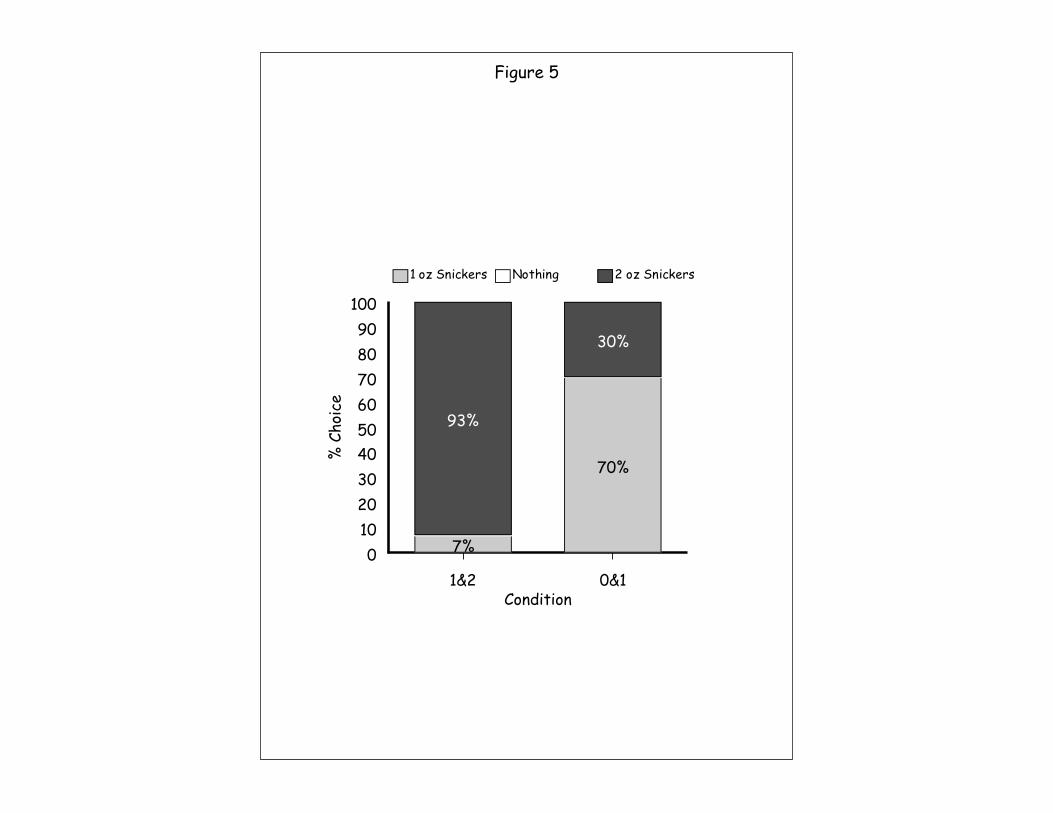
Condition1&2 0&1

% C

hoi

ce

0

10

20

30

40

50

60

70

80

90

100

7%

70%

93%

30%

1 oz Snickers Nothing 2 oz Snickers

Figure 5

Condition5&12 1&8 0&7

% C

hoi

ce

0

10

20

30

40

50

60

70

80

90

100

29% 36%

100%

71%64%

$10 Gift cer Nothing $20 Gift cer

Figure 6

Hershey 0 Hershey 1 Lindt 13 Lindt 14

Aff

ect

0

1

2

3

4

5

4.10

2.82 2.78 2.97

Figure 7

Condition

1&14 0&13 1&14 0&13

% C

hoi

ce

0

10

20

30

40

50

60

70

80

90

100

29%

64%

33%40%

2%

71%

36%

65% 60%

Hershey's Nothing Lindt

Neutral Forced analysis

Figure 8