Embed Size (px)
Citation preview
ABSTRACT
NELSON, PAUL THOMAS. Evaluation of elite exotic maize inbreds for use in long-term
temperate breeding. (Under the direction of Major M. Goodman.)
The U.S. maize (Zea mays L.) germplasm base is narrow. While maize is a very
diverse species, that diversity is not represented in U.S. maize production acreage. Most elite
U.S. maize inbreds can be traced back to a small pool of inbreds that were developed decades
ago. Increased genetic diversity can be obtained through breeding with exotic germplasm,
especially tropical-exotic sources. However, setbacks are often encountered when working
with tropical germplasm due to adaptation barriers. Furthermore, the pool of available
tropical germplasm is large and diverse, making choices of tropical parents difficult. The
maize breeding program at North Carolina State University has begun a large-scale screening
effort to evaluate elite exotic maize inbreds, most of which are tropical-exotic in origin. The
purpose of this research was to: 1) generate comparative yield-trial data for over 100 elite
exotic maize inbreds, 2) determine the relative effectiveness of various testcross regimes, 3)
identify sources of gray leaf spot (GLS) resistance among these elite exotic inbreds, and 4)
promote the use of exotic maize germplasm to broaden the genetic base of U.S. maize.
Over 100 elite exotic maize inbreds were obtained from various international
breeding programs. They were tested in replicated yield trials in North Carolina as 50%-
exotic testcrosses by crossing them to a broad-base U.S. tester of Stiff Stalk (SS) × non-Stiff
Stalk (NSS) origin. The more promising lines additionally entered 25%-tropical testcrosses
with SS and NSS testers and were further evaluated in yield-trials. A dozen tropical inbred
lines performed well overall—CML10, CML108, CML157Q, CML258, CML264, CML274,
CML277, CML341, CML343, CML373, Tzi8, and Tzi9. Inbred lines CML157Q, CML343,
CML373, and Tzi9 did not show significant line × tester interaction. Furthermore, it was
determined that testcrossing to a single broad-based tester will suffice for initial screening
purposes, allowing for elimination of the poorest performing lines. Testcrossing to additional
SS and NSS testers may be of value when determining where the better performing materials
will fit into a breeding program. It was further determined that most tropical lines can
effectively be evaluated at the 50%-tropical level because many of the problems typically
associated unadapted tropical material were minimized through a single testcross to an
adapted tester.
Each of the exotic lines was screened for GLS resistance either as inbreds per se, as
testcrosses, or both. Many of the inbreds showed high levels of GLS resistance, including
several lines that have good yield potential. These lines include CML108, CML258,
CML274, CML277, CML343, and Tzi16.
The results presented in this thesis provide temperate breeders with information on a
sizable pool of potentially useful exotic maize inbred lines. These lines certainly deserve
further attention in breeding efforts to broaden the U.S. maize germplasm base. Many are
already being used at North Carolina State University in both exotic × temperate and exotic ×
exotic breeding crosses and populations.
EVALUATION OF ELITE EXOTIC MAIZE INBREDS FOR USE IN LONG-TERM TEMPERATE BREEDING
by
PAUL THOMAS NELSON
A thesis submitted to the Graduate Faculty of North Carolina State
University in partial fulfillment of the requirements for the degree of Master of
Science
CROP SCIENCE
Raleigh – 2006
APPROVED BY:
_______________________________ _______________________________ Dr. Cavell Brownie Dr. James B. Holland Statistics Crop Science
_______________________________ Dr. Major M. Goodman
Chair of Advisory Committee Crop Science
ii
BIOGRAPHY
Paul Thomas Nelson is the sixth of nine children born to Thomas K. and Susan O.
Nelson. He was born on the 26th of May, 1980, in Manhattan, Kansas where he spent the
first 17 years of his life. At an early age he came to appreciate rural Kansas life, spending
countless hours in the large family garden or mowing hay in the family’s 30 acre pasture. At
the beginning of his senior year his family moved to Utah, where he finished high school. In
the fall of 1998 Paul’s post high school education began at Ricks College in Rexburg, Idaho
where he enrolled in the Department of Agronomy. After completing one year at Ricks
College, Paul put his academic ambitions on hold for two years to serve full-time as a
missionary for the Church of Jesus Christ of Latter-Day Saints. He was assigned to serve in
Phnom Penh, Cambodia, where he learned the language and customs of the Cambodian
people while delivering the message of the restored gospel of Jesus Christ. Upon returning
home in 2001, he resumed his education at Rexburg, Idaho where Ricks College had now
become Brigham Young University-Idaho. There he completed his Associates Degree in
Agronomy and graduated in the spring of 2002. That same year, before transferring to
Brigham Young University in Provo, Utah, Paul embarked on an 8-month internship in
Waterloo, Iowa, where he worked at a soybean research station for Pioneer Hi-Bred
International, Inc. This internship introduced Paul to applied research in plant breeding. He
enjoyed the experience so much that he did another internship for Pioneer the following
summer at a corn research station in Ithaca, Michigan.
Paul finished his undergraduate work at BYU-Provo and graduated in April of 2004.
While doing his undergraduate work he enjoyed working in a plant genetics lab under the
direction of Drs. Rick Jellen and Jeff Maughan. Under their supervision he engaged in
DNA-marker work on quinoa (Chenopodium quinoa).
During his senior year at BYU, Paul met Lisa Marie Ewert, an attractive young nurse
from California who was not only stunningly beautiful but gainfully employed as an RN.
The two courted and were married in June of 2004. Immediately following their marriage
Paul and Lisa moving to Raleigh, North Carolina, where Paul began his graduate career in

iii
the NCSU corn breeding program under the mentorship of Dr. Major M. Goodman. While in
North Carolina, Paul and Lisa expanded their family by one. Only hours after this thesis was
submitted to Paul’s committee for review, Lisa gave birth to their first child, Samuel Thomas
Nelson.
iv
ACKNOWLEDGEMENTS
I am indebted to many individuals who have enabled the completion of this thesis.
Foremost, I am grateful to my advisor, Dr. Major M. Goodman, for his mentorship the past
two years. Dr. Goodman is a caring and patient individual whose vested interest in my
success has been very evident. He has patiently answered my questions and taken the time to
share his wisdom and expertise with me. It is because of him that I have opted to pursue a
Ph.D. under his continued mentorship, despite his satirical proclamation “sometimes people
just make poor decisions”.
I am also grateful to the other two members of my committee, Dr. Jim Holland and
Dr. Cavell Brownie. Dr. Holland has always been willing to answer my questions and
provide advice about my research; his opinions are highly valued. Further, his energetic and
outgoing nature makes association with him and his students (appropriately dubbed “team-
corn”) quite enjoyable. Through Dr. Brownie’s instruction, both in the classroom and one-
on-one, I have learned the statistical skills necessary for proper data analysis. I feel
privileged to have worked with Dr. Brownie for two main reasons: first, her exceptional
knowledge of field-data analyses and second, her kind nature and willingness to assist
students.
My graduate education was funded through a fellowship from Pioneer Hi-Bred
International, Inc. and by the Initiative for Future Agriculture and Food Systems Grant no.
2001-52101-11507 from the USDA Cooperative State Research, Education, and Extension
Service. The contribution of these institutions to my research and education is greatly
appreciated.
As a member of the NCSU corn breeding program, my research would not have been
possible without the assistance of outstanding technicians and fellow graduate students. Bill
Hill’s behind-the-scene management of field operations and data management has been
invaluable to my project. Wayne Dillard has contributed countless man-hours to my project,
spending nights and even weekends on the road planting and harvesting thesis experiments.

v
Joe Hudyncia and Roy Ray have also provided valuable support, man-hours, and training to
my research.
I owe sincere gratitude to Mike Jines, my fellow graduate student in the NCSU corn
breeding program. Mike has helped me transition into the life of a graduate student and corn
breeder. On my first day in the program, he explained to me the difference between a Stiff
Stalk and a Lancaster line. He helped me write my first SAS program, gave me advice about
which classes to take (and which classes not to take) and showed me the “special places” to
find seed when all other sources failed. Mike has had an exemplary influence on my
education with his enthusiasm for statistical inference and breeding methods. Undoubtedly, I
will be rubbing shoulders with Mike for the rest of my career, an association that I look
forward to.
Finally, I owe deepest gratitude to my family and especially my sweetheart and best
friend, my wife, Lisa. She has supported me through many late nights when I had to analyze
data or study for exams, or evenings and weekends that I have spent in the field. She has
kept my sanity in check; continually reminding me that there is more to life than corn.
Coming home from work is always exciting with her and our new little boy, Sam, there to
meet me.
vi
TABLE OF CONTENTS Page LIST OF TABLES................................................................................................................. viii LIST OF FIGURES ...................................................................................................................x CHAPTER I – Literature Review..............................................................................................1
Origin of Maize..............................................................................................................1 Ancesteral Origin...............................................................................................1 Temporal and Geographic Origin .....................................................................2 Races of Maize...............................................................................................................3 Maize Diversity in the U.S.............................................................................................3 Pre-hybrid Maize Diversity in the U.S...............................................................4 The Advent of Hybrid Maize ..............................................................................5 Diversity within Modern U.S. Maize..................................................................6 Influential Central and Southern Corn Belt Inbred Lines..............................................7 B73 .....................................................................................................................7 B14/B14A ...........................................................................................................7 Mo17 ..................................................................................................................8 Oh43...................................................................................................................8 B37 .....................................................................................................................8 Diversifying the U.S. Maize Germplasm Base..............................................................9 Modern Statistical Methods and Experimental Design ...............................................11 References....................................................................................................................13
CHAPTER II – Selecting Among Available, Elite Tropical Maize Inbreds for Use in Long-
Term Temperate Breeding ...........................................................................................24 Abstract ........................................................................................................................25 Introduction..................................................................................................................26 Materials and Methods.................................................................................................27 Results and Discussion ................................................................................................29 Conclusion ...................................................................................................................32 References....................................................................................................................33
CHAPTER III – Selecting Among Available Elite Exotic Maize Inbreds for Use in Long-
Term Temperate Breeding II .......................................................................................40 Introduction..................................................................................................................40 Materials and Methods.................................................................................................41 Germplasm Selection .......................................................................................41 Yield Trial Evaluation......................................................................................42 Data Analysis ...................................................................................................44
vii
Results and Discussion ................................................................................................46 Entry Performance...........................................................................................46 Line × Tester Interaction .................................................................................46 Genotype × Environment Interaction ..............................................................47 Tester Correlation............................................................................................48 Conclusion ...................................................................................................................48 References....................................................................................................................50
CHAPTER IV – Gray Leaf Spot Evaluation of Elite Tropical Maize Inbreds........................57
Introduction..................................................................................................................57 Materials and Methods.................................................................................................58 Germplasm Selection .......................................................................................58 Experimental Design........................................................................................60 Data Analysis ...................................................................................................61 Results and Discussion ................................................................................................62 Entry Performance...........................................................................................62 Gray Leaf Spot and Yield Correlation .............................................................62 Conclusion ...................................................................................................................63 References....................................................................................................................64
APPENDIX A – Supporting Material for Chapter II...............................................................74 Line × Tester Interaction..............................................................................................74 APPENDIX B – Supporting Material for Chapter III .............................................................76 Results and Discussion ................................................................................................76 Subsets of Exotic Entries..................................................................................76 Stability Analysis Using an Environmental Index ...........................................78 References....................................................................................................................78 APPENDIX C – Supporting Material for Chapter IV ...........................................................108 APPENDIX D – Common and Southern Rust Evaluation of Exotic Inbreds .......................111
viii
LIST OF TABLES
Page CHAPTER II Table 2.1 Lines used, germplasm sources, and seed sources..............................................35 Table 2.2 Means of tropical lines × U.S. testers; 50% and 25%-tropical topcrosses .........36 Table 2.3 Lines selected using four selection truncation points for yield...........................38 Table 2.4 Spearman’s coefficients of correlation for entries ranked by yield across testers and years ..................................................................................................39 CHAPTER III Table 3.1 Experimental lines and origin .............................................................................53 Table 3.2 Preferred analysis used for each trait across all locations within years..............54 Table 3.3 25% and 50%-exotic entry means from 10 environments 2003 – 2005 .............55 Table 3.4 Line × tester interactions for yield given as deviations from the mean ..............56 CHAPTER IV Table 4.1 Breeding programs / breeders and line prefixes .................................................67 Table 4.2 GLS ratings of 102 experimental inbreds and 5 checks with standard errors and # of environments ..............................................................................68 Table 4.3 GLS ratings of testcrosses and 15 commercial checks .......................................69 APPENDIX A Table A.1 Line × tester interactions for yield ......................................................................74 Table A.2 Line × tester interactions for yield given as deviations from the mean ..............75 APPENDIX B Table B.1 Entries and years tested.......................................................................................79 Table B.2 2001 entry means. Data from Clayton, Lewiston, Plymouth, and Sandhills, NC .............................................................................................................................82 Table B.3 2002 entry means. Data from Clayton, Lewiston, Plymouth, and Sandhills, NC .............................................................................................................................83 Table B.4 2003 entry means. Data from Clayton and Lewiston, NC. 50% and 25%-exotic testcrosses ...........................................................................................................84 Table B.5 2004 entry means. Data from Clayton, Lewiston, Kinston, and Sandhills, NC.
50% and 25%-exotic testcrosses ........................................................................86 Table B.6 2005 entry means. Data from Clayton, Lewiston, Plymouth, and Sandhills, NC.
50% and 25%-exotic testcrosses.........................................................................88
ix
Table B.7 Means for the subset of 50%-exotic entries from 14 environments 2002 – 2005 .............................................................................................................................90 Table B.8 Entry means for 50% and 25%-exotic testcrosses ..............................................91 Table B.9 Line × tester interactions for yield ......................................................................96 Table B.10 Significance levels (α = .05) of genotype by environment interactions within Years ...................................................................................................................97 Table B.11 Spearman’s coefficient of rank correlation for traits across environments ........97 Table B.12 Spearman’s coefficients of correlation for entries ranked across testers............98 Table B.13 2001 Environmental Index..................................................................................99 Table B.14 2002 Environmental Index..................................................................................99 Table B.15 2004 Environmental Index................................................................................100 Table B.16 2005 Environmental Index................................................................................101 APPENDIX D Table D.1 Common rust disease ratings ............................................................................112 Table D.2 Southern rust disease ratings.............................................................................113
x
LIST OF FIGURES
Page CHAPTER I Figure 1.1 U.S. maize yields from 1866 – 2006...................................................................23 CHAPTER IV Figure 4.1 Inbred per se GLS ratings × testcross yield, entries from Nelson et al. (2006). Tester = LH132 × LH51. Coefficient of correlation, r = -0.08..........................71 Figure 4.2 Inbred per se GLS ratings × testcross yield, entries from Chapter 3 of this thesis. Tester = LH132 × LH51. Coefficient of correlation, r = -0.03..........................72 APPENDIX B Figure B.1 Consistency of performance stability analysis for entries tested in 2001. Entries that consistently (low standard deviation (SD) of entry rank) ranked high (low mean rank) are considered stable......................................................................102 Figure B.2 Consistency of performance stability analysis for entries tested in 2002. Entries that consistently (low standard deviation (SD) of entry rank) ranked high (low mean rank) are considered stable......................................................................103 Figure B.3 Consistency of performance stability analysis for entries tested in 2004. Entries that consistently (low standard deviation (SD) of entry rank) ranked high (low mean rank) are considered stable......................................................................104 Figure B.4 Consistency of performance stability analysis for entries tested in 2005. Entries that consistently (low standard deviation (SD) of entry rank) ranked high (low mean rank) are considered stable......................................................................105 Figure B.5 Yield trial and gray leaf spot (GLS) screening locations given with 30-year average precipitation levels across the state of North Carolina. The precipitation data were complied from the National Climate Data Center monthly precipitation totals and interpolated using a linear kriging algorithm. Interpolations were run on 160 gauging stations using 500 foot square grid cells ................................106 Figure B.6 Yield trial and gray leaf spot (GLS) screening locations given with soil systems across the state of North Carolina.....................................................................107 APPENDIX C Figure C.1 Testcross GLS ratings × testcross yield, entries from Nelson et al. (2006). Coefficient of correlation, r = -0.13..................................................................109 Figure C.2 Testcross GLS ratings × testcross yield, entries from Chapter 3 of this thesis. Coefficient of correlation, r = -0.08..................................................................110
– CHAPTER I –
Literature Review
Origin of Maize
The origin of maize, both ancestral and geographic, has been a topic of disagreement
within the maize community for many years (Doebley, 2004; Iltis, 2000; Wilkes, 2004). This
is partially because, unlike most cultivated crops, there is no “wild” maize. There is general
agreement that teosinte, of the genus Zea, and the closest known relative to maize, played
some role in maize evolution, though there are still varying opinions on what that role was
(Doebley, 1990; Galinat, 1988; Goodman, 1988; Iltis, 2000; Wilkes, 2004). However, today
the “teosinte hypothesis,” which claims that maize was domesticated from the Mexican
annual teosinte, Z. mays ssp. Parviglumis and that the origin of domestication is near the
Balsis River drainage in Mexico (Doebley, 2004; Matsuoka, 2005; Vigouroux et al., 2005) is
widely accepted. There is general consensus in the literature that maize was domesticated
between 7,000 and 10,000 years ago (Doebley, 2004; Galinat, 1988; Goodman, 1988;
Wilkes, 2004).
Ancestral Origin
Goodman (1988) summarized three predominant hypotheses on the evolution of teosinte
and maize:
1) Teosinte and maize diverged from a hypothetical unknown common ancestor or “wild
maize”.
2) Maize was domesticated from teosinte, i.e. teosinte is “wild maize”. Also known as
the teosinte hypothesis.
3) Annual teosinte is descendant from a maize × perennial teosinte cross.
Wilkes (2004) outlines three similar theories. Iltis (2000) provides a history of the various
theories on the origin of maize and of the controversy surrounding them.
With the advent of isozyme and DNA marker technology in the 1980’s much of the
controversy surrounding the origin of maize was put to rest. Doebley led the way with
isozyme data by which he began to establish the teosinte hypothesis as the dominant
2
explanation for the origin of maize (Doebley, 1990; Doebley et al., 1987). Specifically, this
theory is that maize was derived through a single domestication event of the Mexican annual
teosinte, Z. mays ssp. parviglumis (Doebley, 2004; Matsuoka et al., 2002). This theory has
become accepted in the literature as the dogma of maize evolution (Doebley, 2004;
Matsuoka, 2005; Vigouroux et al., 2005). Today, much of the genetic work in maize
evolution is aimed at identifying single genes and gene families that explain the
morphological differences between teosinte and maize (Clark et al., 2004; Doebley and Stec,
1993; Doebley, 2004 ; Dorweiler et al., 1993; Dorweiler and Doebley, 1997; Wang et al.,
2005; White and Doebley, 1999). However, as Wilkes points out (Wilkes, 2004), a few
researchers are reluctant to fully adopt the teosinte hypothesis (Eubanks, 1995, 2001a, 2001b,
2001c; Goodman, 1965; Goodman, 1976; Goodman, 1988; Wilkes and Goodman, 1995;
Bird, personal communication; Goodman, personal communication). The archeological
evidence does not support the teosinte hypothesis as well as the molecular evidence. For
example, maize cobs dating to ≈ 6000 B.P. do not show the morphological characteristics
expected from a teosinte derivative (Brown, 1978; Wilkes, 2004). However, cobs dating to ≈
3000 B.P. show greater resemblance to teosinte which may suggest a post-domestication
introgression of teosinte into maize (Wilkes, 2004).
Temporal and Geographic Origin
There is general consensus in the literature that maize was domesticated between
7,000 and 10,000 years ago (Doebley, 2004; Galinat, 1988; Goodman, 1988; Wilkes, 2004).
However, the geographic origin of domestication, like the ancestral origin, is speculative.
Mangelsdorf (1974) introduced the idea of maize lineages from six different geographical
regions ranging from Mexico to South America. Many advocate a Mexican origin because
teosinte, the closest relative to maize, is essentially restricted to Mexico (Galinat, 1988;
Goodman, 1988; Wilkes, 2004). Supporters of the teosinte hypothesis accept the Balsas
River drainage in southwestern Mexico as the cradle of maize domestication (Matsuoka,
2005). This is the location of the populations of teosinte ssp. parviglumis that most closely
resemble maize in isozyme and microsatellite analyses (Doebley, 1990; Matsuoka et al.,
2002). Thus, the Balsas River drainage is becoming more widely accepted in the literature as
the geographic origin of domestication.
3
The dispute over the origin of maize is anything but settled, though the teosinte
hypothesis currently reigns in popularity. Study of the origin of maize is interdisciplinary,
including geographical, archeological, botanical, historical, and genetic evidences (Brown,
1978; Goodman, 1988; Wilkes, 2004). To exclude evidence from any one of these
disciplines may limit one’s ability to understand the origin of maize.
Races of Maize
There is great genetic diversity found within maize (Wright et al., 2005). In the past
century there have been numerous monographs and surveys on the races of maize.
Sturtevant (1899) divided maize varieties into six “species groups” based on kernel
morphology. Anderson and Cutler (1942) recognized the artificial nature of these groupings
and called for a more comprehensive study of the races of maize. Thereafter, the Rockefeller
Foundation and the National Academy of Sciences published a series of monographs that
identified over 300 races of maize in the Americas (Brieger et al., 1958; Brown, 1960; Grant
et al., 1963; Grobman et al., 1961; Hatheway, 1957; Paterniani and Goodman, 1977; Ramirez
et al., 1960; Roberts et al., 1957; Timothy et al., 1961, 1963; Wellhausen et al., 1952, 1957).
Goodman and Bird (1977) and Goodman and Brown (1988) provide the most comprehensive
summaries to date of the aforementioned monographs. A series of publications by Goodman,
Stuber, and associates represent the most complete molecular surveys on the genetic diversity
among the races of maize based on isozyme markers (Bretting et al., 1987, 1990; Goodman
and Stuber, 1983; Goodman et al., 1980; Sanchez and Goodman, 1992a, 1992b; Sanchez et
al., 2000a, 2000b, 2006).
Maize Diversity in the U.S.
The U.S. is the world leader in maize production (USDA, 2005a) with over 80
million acres of maize grown in 2005 (USDA, 2005b). However, very little of the diversity
that is found among the races of maize is represented in U.S. production acreage. Goodman
and Brown (1988) classified 10 broad racial complexes of maize that have, at some time,
been used in the U.S. However, today U.S. maize production is composed of basically two
races, the Northern Flints and Southern Dents. Corn Belt Dents, which are a product of
4
repeated hybridization of the Northern Flints and Southern Dents, are sometimes considered
a third race (Brown, 1947).
Pre-hybrid Maize Diversity in the U.S.
Before the advent of hybrid maize, there were hundreds of open pollinated varieties
of maize grown throughout the U.S. Pre-20th century farmers selected the best ears at harvest
to use as seed the following season. Selection criteria varied among growers as did the niche
environment in which selections were being made. This system of maize production and
farmer-selection promoted diversity across the U.S. Corn Belt. This diversity probably
peaked around 1900, the same time that corn shows were gaining popularity across the Corn
Belt (Wallace and Bressman, 1937). The purpose of the corn shows was to recognize
varieties that showed the greatest yield potential. Wallace and Bressman (1937) describe the
ideal corn show ear as being “10 inches long, 7½ inches in circumference, with eighteen to
twenty-two rows packed together on the cob and carried out over the tip and well-rounded
butt” (p. 251). However, the corn shows were flawed because yield potential was judged by
individual ear and kernel morphology, not agronomic yield. In fact, corn shows may have
had an opposite affect on maize production than was originally intended. Often the prize-
winning corn-show varieties did not yield as well as varieties that were judged inferior by
corn-show standards (Wallace and Brown, 1988). Unfortunately, through the popularity of
corn shows and prize-winning varieties, many growers abandoned their traditional varieties
and adopted the sometimes inferior “prize corns”.
In time, growers realized that the prize-winning varieties from the corn shows were
not necessarily the highest yielding varieties (Wallace and Brown, 1988). By 1910, variety
yield trials began replacing corn shows and a few noted varieties were gaining popularity
throughout the Corn Belt, varieties such as Reid Yellow Dent, Krug, Lancaster, and Leaming
(Goodman and Brown, 1988). These superior, higher yielding varieties, replaced many of
the traditional varieties. Subsequently, much of the genetic diversity that had accumulated
through centuries varietal differentiation across the Corn Belt was lost (Wallace and Brown,
1988).
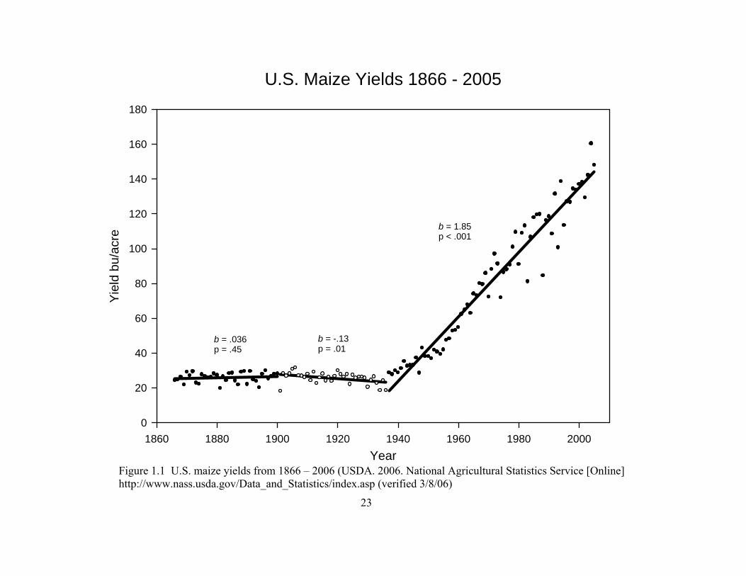
It is interesting to note that U.S. maize yields reached a plateau around 1900 and
subsequently began a downward trend during the first three decades of the 20th century.
5
Based on USDA data from 1866 – 2005 (USDA, 2006), maize yields in the U.S. were
improving from 1866 – 1900 (Fig. 1.1). However, from 1900 – 1936 yields steadily
decreased across the Corn Belt, a trend that was clearly established before the droughts of the
early to mid 1930’s. The exact cause of this trend is open to speculation. However, it is
difficult to attribute a 30 year trend merely to weather conditions or “bad luck”. Genetic
variation for yield across the Corn Belt obviously was not exhausted as evidenced by the
tremendous gains seen since the 1930’s. However, genetic variation within open pollinated
maize populations may have been limited, especially in light of the 20 year influence of the
corn shows which promoted uniformity, the antithesis of the diversity that drives productivity
in an open pollinated maize population. This, coupled with the superficial definition of yield
that was praised by the corn shows, may have been a contributor to this temporary agronomic
downslide in maize productivity.
The Advent of Hybrid Maize
Hybrid vigor in maize was first noted around the year 1871 by Charles Darwin who
observed height differences between inbred parents and their cross-bred progeny (Darwin,
1877). W. J. Beal, a close follower of Darwin (Wallace and Brown, 1988), was intrigued by
this finding and subsequently crossed two divergent dent corns, becoming the first individual
to make controlled pollinations in maize with the expressed purpose of increasing yields
through hybrid vigor (Beal, 1878). In 1908 George Harrison Shull noted the value of
inbreeding in maize improvement, stating that “the object of the corn-breeder should not be
to find the best pure-line, but to find and maintain the best hybrid combinations” through
inbreeding (Shull, 1908). His “pure line” theory of maize breeding (Shull, 1909) was a
highly significant contribution to maize improvement, although its agricultural significance
was not immediately realized. Early inbreeding efforts with open pollinated maize varieties
were plagued by severe inbreeding depression (Jones, 1918). This limited the practicality of
hybrid maize production. Other maize scientists of the time were also actively inbreeding
maize and observing the effects. E.M. East was one such prominent individual who was
especially intrigued by Shull’s work and had actually observed similar results in his own
research (Crabb, 1947). One of East’s students was D.F. Jones, another very influential
individual in maize breeding in the 20th century.
6
It wasn’t until D.F. Jones introduced the double cross in 1918 that large-scale hybrid
maize production became possible (Jones, 1918). Some varieties survived the inbreeding
process and others did not. A few outstanding varieties, including Reid Yellow Dent,
Minnesota 13, Lancaster Sure Crop, and Leaming Corn, served as the genetic foundation for
hybrid maize (Baker, 1984; Goodman and Brown, 1988). This had a bottlenecking effect on
the genetic diversity of U.S. maize because many open pollinated varieties that did not
survive inbreeding were left behind and lost forever.
Diversity within Modern U.S. Maize
In the period from 1956 to 1986, the American Seed Trade Association conducted six
surveys on the breadth of the U.S. maize germplasm base (Darrah and Zuber, 1986; Sprague,
1971; Zuber, 1975; Zuber and Darrah, 1980). The most recent survey (Darrah and Zuber,
1986) found that 5 inbred lines, B73, A632, W117, Mo17, and CM174, were each used per
se in more than 1% of the total U.S. seed requirement in 1984, the greatest being B73 which
was used in 11% of the total U.S. seed requirement. Smith (1988) conducted an isozyme
survey of the U.S. maize germplasm base. He concluded that inbred lines B73, A632, Oh43,
and Mo17 were the major contributors to U.S. maize germplasm. Subsequent surveys of
germplasm usage have been unsuccessful due to seed labels that prohibit genotyping and the
increased reluctance of private companies to provide relevant information.
Baker (1984), of Pioneer Hi-Bred international, Inc., reported what he and Bill
Ambrose (a long-time corn breeder at Pioneer Hi-Bred International, Inc.) believed to be the
seven most widely used hybrid combinations in the U.S., they were:
1) B73 × Mo17
2) A632 × H993H95
3) Mo17 × A634
4) B73 × PA91
5) B73 × MS71
6) Mo17 × CM105
7) A632 × W117.
Baker also provides historical background on each of the lines involved in these hybrids.
Goodman (Goodman, 1992) concluded that inbred lines B14A, B37, B68, B73, B84 (female
7
lines) and C103, Mo17, and Oh43 (male lines) have essentially served as the primary
germplasm source for U.S. maize breeding programs for decades. Troyer (2004, 1999)
provides background and historical information on the most prominent lines in use in the
U.S.
Influential Central and Southern Corn Belt Inbred Lines
As noted, several inbred lines stand out in the literature as being highly influential in
U.S. maize breeding and production. Brief histories of some of these lines are provided in
the following:
B73
Inbred line B73 has been the most widely used inbred line in breeding and production
since its release in 1972 (Baker, 1984; Darrah and Zuber, 1986). It was developed at Iowa
State University out of cycle 5 of the Iowa Stiff Stalk Synthetic (Russell, 1972). It was
actually discarded one year but was quickly retrieved after yield data were analyzed (Troyer,
1999). Despite problems with insect and disease susceptibility, it has excellent yield
potential. It is most famous for its use in the very popular hybrid B73 × Mo17. Relative
maturity of B73 hybrids ranges from 110 to 130 days (Baker, 1984).
B14/B14A
Inbred line B14 was developed at Iowa State University from the first cycle of
recurrent selection of the Iowa Stiff Stalk Synthetic. It was developed by G.F. Sprague and
released in 1953 (Troyer, 1999). It provides high yield, fast ear dry-down, resistance to root
and stalk lodging, and resistance to northern corn leaf blight (Helminthosporium turcicum
Pass.) (Russell et al., 1971). B14, however, is susceptible to corn leaf rust (Puccinia sorghi
Schw.) which prompted the development and release of B14A in 1962, which is nearly
identical to B14, but carries resistance to corn leaf rust. B14A was developed through
backcrossing to Cuzco (Cuzco × B14 (8)) (Russell et al., 1971). B14 and derived-line
hybrids are generally earlier than 110 days relative maturity (Baker, 1984). B14 is a parent
of such influential inbred lines as A632 [(Mt42 × B14)B143], A634 [(Mt42 × B14) self
B142], CM105 [V3 × B142], and CM174 [V3 × B142] (Coors et al., 1993). B68 is another
8
influential line that was derived through three backcrosses to B14 (Russell et al., 1971;
Goodman, 1998).
Mo17
Inbred line Mo17 was developed under the direction of M. S. Zuber at the University
of Missouri as part of C. O. Grogan’s thesis project. It was released in 1964 (Troyer, 1999;
Zuber, 1973). It is most famous for its use in hybrid combination with B73. Mo17 was
developed out of CI187-2 × C103. Inbred line CI187-2 was selfed out of Krug Reid by L.
Pfister and C103 was developed by D.F. Jones who selfed it out a Lancaster population that
was obtained directly from Noah L. Hershey’s farm near Parkesburg, Pennsylvania (Baker,
1984; Troyer, 1999). C103 was possibly the first widely used Lancaster line (Goodman,
personal communication). Relative maturity of Mo17 hybrids is similar to that of C103, 95
to 125 days. (Baker, 1984; Zuber, 1973).
Oh43
Inbred line Oh43 was developed by Glenn H. Stringfield at the Ohio Experiment
Station and released in 1949 (Troyer, 1999). It was selfed out of W8 × Oh40B. W8 is ½
Minnesota 13, ½ Funk Yellow Dent and Oh40B was developed from the Lancaster Synthetic
(Coors et al., 1993). Though Oh43 is not included in Darrah and Zuber’s 1986 survey, they
do note that it has probably a made a significant contribution through private lines such as
LH38 (Holden’s Foundation Seed). Smith (1988) likewise recognized the contribution of
Oh43 through the popular private lines LH38 and LH98.
B37
Like B14, inbred line B37 was developed at Iowa State University from the first cycle
of recurrent selection on the Iowa Stiff Stalk Synthetic (Russell et al., 1971). It was
developed by G.F. Sprague and released in 1958 (Troyer, 1999). B37 replaced the older B14
and it itself was eventually largely replaced by B73 (Baker, 1984; Goodman, personal
communication). It is reported by Darrah and Zuber (1986) as being used in .3% of the total
seed requirement in 1984. B37 hybrids range in maturity from 115 to 130 days (Baker,
1984).
9
Diversifying the U.S. Maize Germplasm Base
For years, maize breeders have advocated breeding with tropical germplasm as a
means of diversifying the U.S. maize germplasm base. Melhus (1948) called for a critical
study of Latin American maize, noting that such material could provide useful variants in
disease, insect, drought, heat, and cold resistance. Brown (1953), in a review of germplasm
sources for U.S. maize improvement, addressed the issue on a global basis. Wellhausen
(1956) forecasted a yield plateau in U.S. maize improvement, stating that a “point of
diminishing returns has now been reached ..., corn breeders will need to look elsewhere for a
new source of yield genes.” In 1965 Wellhausen reiterated the value of exotic sources of
germplasm and presented data on race evaluations. Lonnquist (1974) called for the
development of breeding pools from tropical and tropical × temperate germplasm, and noted
the discouragement of breeders who had failed in their efforts to breed with tropical
germplasm because their selection of tropical parents had essentially been “random”. Brown
(1975), in the wake of the 1970 southern corn leaf blight epidemic (Horsfall et al., 1972),
reviewed the state of the U.S. maize germplasm base and listed some of the more promising
sources of exotic germplasm—Coastal Tropical Flint, Tuxpeño, Tuson, Tiquisate Golden
Yellow, Cuban Flint, Chandelle, Haitian Yellow, and the ETO synthetic. Stuber (1978)
suggested that “every effort should be made to widen the corn germplasm base in U.S.
breeding programs,” and presented screening results of a wide range of exotic maize races
from Latin America. In more recent years the charge has been led by Goodman (Goodman,
1990; Goodman, 1992; Goodman, 1998; Goodman, 1999; Goodman, 2004; Goodman and
Carson, 2000; Goodman et al., 2000) and students out of his program at North Carolina State
University (Castillo-Gonzalez and Goodman, 1989; Hawbaker et al., 1997; Holland, 1994;
Holland and Goodman, 1995, 2003; Holland et al., 1996; Holley and Goodman, 1988; Lewis
and Goodman, 2003; Nelson et al., 2006; Tallury and Goodman, 1999; Uhr and Goodman,
1995a, 1995b).
Despite the historical emphasis that has been placed on diversifying U.S. maize with
exotic germplasm, there is currently very little tropical germplasm represented in private U.S.
maize breeding programs (Goodman, 1999). Goodman (1998) surveyed private breeding
programs in the U.S. and found that there was an increase in the use of exotic germplasm
10
from less than 1% in 1984 to 2.9 % in 1996. While the increase is notable, the underlying
numbers are still quite low. Furthermore, only one tenth of the exotic germplasm referred to
in that study was of tropical origin. According to Goodman (1998), most exotic germplasm
used in the U.S. has two sources, B68 and the French lines F2 and F7. Inbred line B68 is an
Iowa State inbred that was developed from backcrossing Maiz Amargo with B14. Maiz
Amargo is an Argentine cultivar that was discovered in the 1930s and it and its derivatives
are used in many breeding programs as a source of insect resistance. Inbred lines F2 and F7
were derived from the open-pollinated French cultivar Lacaune and provide improved
emergence in cold, wet conditions (Goodman, 1998; 1999). Tropical germplasm is typically
used only as a source of disease or insect resistance introduced through backcrossing.
While there is still very little exotic germplasm found in maize production acreage in
the U.S. today, there are substantial efforts being made by some in the maize community to
incorporate exotic maize germplasm. The maize breeding program at North Carolina State
University has been working with tropical germplasm for nearly 25 years. NC State provides
an ideal environment for a long-term breeding program with tropical maize given its southern
location and its historical emphasis on maize breeding. Wellhausen (1956) noted that maize
breeding programs in the South, with climate and growing conditions midway between those
of Mexico and the Corn Belt, would provide a valuable service to the Corn Belt and local
growers through the incorporation of tropical material. This is precisely what the NC State
maize breeding program has attempted, producing tropical inbreds that are adapted to
southern growing conditions and competitive with elite commercial inbreds. To date, over
45 NC lines have been released that are of partial or all-tropical origin (MBS Genetics,
2005).
Further efforts in diversifying the U.S. maize germplasm base are being carried out
through the Germplasm Enhancement of Maize (GEM) project, a private/public collaborative
breeding project sponsored by the USDA (Salhuana, 1994). The program was proposed as a
follow-up to the Latin American Maize Project (LAMP) which evaluated over 12,000
accessions from 12 countries throughout North, Central, and South America (Pollak, 2003;
Salhuana et al., 1991). Through GEM, exotic lines and accessions are crossed with elite
proprietary U.S. inbreds for line-development purposes. GEM involves the cooperation of
11
approximately 20 private companies and so far 36 GEM-derived lines have been released
(Balint-Kurti et al., 2006; Blanco et al., 2005; Carson et al., 2006).
While the breeding efforts through GEM and at NC State are major steps forward in
maize germplasm enhancement, in many aspects the programs will not have succeeded until
larger percentages of exotic germplasm are being grown in production acreage across the
U.S. Achieving success in this light is a formidable task for two reasons. First, exotic
materials are several decades behind elite U.S. materials in overall improvement. For
example, in 1948 when maize breeding programs across the U.S. were in their second or
third cycles of recurrent selection, and hybrid maize production across the U.S. was
approaching 100%, the Rockefeller Foundation, the only institution of its kind in Mexico,
was releasing its first hybrids (Fitzgerald, 1986). Second, even the most elite tropical maize
lines must overcome photoperiod and other adaptation barriers if they are to be used in
temperate breeding efforts. These obstacles certainly highlight the long-term nature of
working with exotic germplasm. This was certainly realized by the early maize breeders like
Melhus (1948), who called for young breeders to take on the work of developing tropical
synthetics and populations.
Modern Statistical Methods and Experimental Design
The significant advancements in breeding methodology within maize and other crops
in the early to mid part of the 20th century were paralleled by advancements in statistical
analysis and experimental design. Agricultural experiments were the vehicle by which much
of modern experimental design was established (Fisher, 1926). Uniformity trials were
frequently used during the early part of the century to explain error variation in field
experiments. This work illuminated the inherent variability that arises in the field from non-
treatment effects. Considerable effort was subsequently devoted to experimental designs that
would accommodate field variation (Fisher, 1926).
The same year that D.F. Jones (1918) introduced the double cross, R.A. Fisher
introduced the word variance into the statistical language with implication to the analysis of
variance components (Box, 1978; Fisher, 1918). In his first edition of “Statistical Methods
for Research Workers”, Fisher (1925) demonstrated the additive property of variance,
12
thereby providing for an estimate of error from its various causes (Anderson and Bancroft,
1952; Robinson, 1987). The analysis of variance quickly became one of the principal
research tools in the biological sciences (Eisenhart, 1947).
The four primary experimental designs that emerged following the birth of the
analysis of variance were (i) the completely randomized design, (ii) the randomized
complete-blocks design, (iii) the latin-square designs, and (iv) the incomplete blocks-designs
(Anderson and Bancroft, 1952). Eisenhart (1947) gives a comprehensive overview of the
uses for the analysis of variance and the assumptions associated with its use.
One class of experimental analysis that emerged at this time was the spatial or
“nearest-neighbor” analyses, which adjust observed values for variation within the field.
Besag and Kempton (1986) give four distinct applications of neighboring plots analysis,
many of which date back to the early to mid part of the 20th century. (1) Adjustment for
fertility trends through systematic arrangements of check plots. This is perhaps the oldest
application of nearest-neighbor analysis (Wiancko, 1914), and is particularly useful when
treatment replication is not possible. (2) Adjustments for fertility trends using a Papadakis or
related analyses that does not require additional checks, but relies on the treatment replication
and neighboring plots to establish trends. (3) Adjustments for competition between plots.
(4) Adjustments for interference between neighboring treatments. Federer and Schlottfeldt
(1954) used covariance to detect row and column gradients in a field trial, a technique
sometimes referred to as a trend analysis. Zimmerman and Harville (1991) introduced an
analysis that models spatial heterogeneity directly, based on the assumption that neighboring
plots will have correlated errors. Brownie et al. (1993) did a comprehensive comparison
among three of these spatial analyses, trend analysis, Papadakis method, and the correlated
errors analysis. Jines et al. (2006) developed software that compares various spatial analyses
and outputs results from the “preferred” analysis, based on various criteria.
13
References
Anderson, E., and H.C. Cutler. 1942. Races of Zea mays. Annals of the Missouri Botanical Garden 29:69-88.
Anderson, R.L., and T.A. Bancroft. 1952. Statistical theory in research. McGraw-Hill Book Company, Inc., New York.
Baker, R. 1984. Some of the open pollinated varieties that contributed the most to modern hybrid corn. Illinois Corn Breeder's School Proc. 20:1-19.
Balint-Kurti, P.J., M. Blanco, M. Millard, S. Duvick, J.B. Holland, M.J. Clements, R.N. Holley, M.L. Carson, and M.M. Goodman. 2006. Registration of 20 GEM maize breeding germplasm lines adapted to the southern USA. Crop Science 46:996-998.
Beal, W.J. 1878. Report of the professor of botany and horticulture. Report Michigan Board of Agriculture:41-59.
Besag, J., and R. Kempton. 1986. Statistical-analysis of field experiments using neighboring plots. Biometrics 42:231-251.
Blanco, M., C.A. Gardner, W. Salhuana, and N. Shen. 2005. Germplasm enhancement of maize project (Gem). Annual Illinois Corn Breeding School Proc 41:22-41.
Box, J.F. 1978. R. A. Fisher, the life of a scientist. John Wiley & Sons, New York.
Bretting, P.K., M.M. Goodman, and C.W. Stuber. 1987. Karyological and isozyme variation in West Indian and allied American mainland races of maize. American Journal of Botany 74:1601-1613.
Bretting, P.K., M.M. Goodman, and C.W. Stuber. 1990. Isozymatic variation in Guatemalan races of maize. American Journal of Botany 77:211-225.
Brieger, F.G., J.T.A. Gurgel, E. Paterniani, A. Blumenschein, and M.R. Alleoni. 1958. Races of maize in Brazil and other eastern South American countries. NAS-NRC Publ. 593. National Academy of Sciences, Washington, DC.
Brown, W.L. 1947. The northern flint corns. Annals of the Missouri Botanical Garden 34:1-29.
14
Brown, W.L. 1953. Sources of germ plasm for hybrid corn. Corn and Sorghum Res. Conf. Proc. 8:11-16.
Brown, W.L. 1960. Races of maize in the West Indies. NAS-NRC Publ. 792. National Acadamy of Sciences, Washington, DC.
Brown, W.L. 1975. A broader germplasm base in corn and sorghum. Corn and Sorghum Res. Conf. Proc. 30:81-89.
Brown, W.L. 1978. Introductory remarks to the session on evolution., p. 87-91, In D. Walden, ed. Maize Breeding and Genetics. Wiley-Interscience, New York.
Brownie, C., D.T. Bowman, and J.W. Burton. 1993. Estimating spatial variation in analysis of data from yield trials: A comparison of methods. Agronomy Journal 85:1244-1253.
Carson, M.L., P.J. Balint-Kurti, M. Blanco, M. Millard, S. Duvick, R.N. Holley, J. Hudyncia, and M.M. Goodman. 2006. Registration of 9 high-yielding tropical by temperate maize germplasm lines adapted for the southern US. Crop Science (in press).
Castillo-Gonzalez, F., and M.M. Goodman. 1989. Agronomic evaluation of Latin-American maize accessions. Crop Science 29:853-861.
Clark, R.M., E. Linton, J. Messing, and J.F. Doebley. 2004. Pattern of diversity in the genomic region near the maize domestication gene tb1. Proceedings of the National Academy of Sciences of the United States of America 101:700-707.
Coors, J.G., J.T. Gerdes, C.F. Behr, W.F. Tracy, J.L. Geadelmann, and M.K. Viney, (eds.) 1993. Compilation of North American maize breeding germplasm. Crop Science Society of America, Inc.
Crabb, A.R. 1947. The hybrid-corn makers: Prophets of plenty. Rutgers University Press, New Brunswick.
Darrah, L.L., and M.S. Zuber. 1986. 1985 United States farm maize germplasm base and commercial breeding strategies. Crop Science 26:1109-1113.
Darwin, C. 1877. The effects of cross and self fertilisation in the vegetable kingdom. D. Appleton, New York.
Doebley, J.F. 1990. Molecular evidence and evolution of maize. Economic Botany 44:6-27.
15
Doebley, J.F. 2004. The genetics of maize evolution. Annual Review of Genetics 38:37-59.
Doebley, J.F., M.M. Goodman, and C.W. Stuber. 1987. Patterns of isozyme variation between maize and Mexican annual teosinte. Economic Botany 41:234-246.
Doebley, J.F., and A. Stec. 1993. Inheritance of the morphological differences between maize and teosinte - comparison of results for 2 F2 populations. Genetics 134:559-570.
Dorweiler, J., A. Stec, J. Kermicle, and J.F. Doebley. 1993. Teosinte-glume-architecture-1 - a genetic-locus controlling a key step in maize evolution. Science 262:233-235.
Dorweiler, J.E., and J.F. Doebley. 1997. Developmental analysis of teosinte glume architecture1: A key locus in the evolution of maize (Poaceae). American Journal of Botany 84:1313-1322.
Eisenhart, C. 1947. The assumptions underlying the analysis of variance. Biometrics 3:1-21.
Eubanks, M. 1995. A cross between 2 maize relatives - Tripsacum dactyloides and Zea diploperennies (Poaceae). Economic Botany 49:172-182.
Eubanks, M.W. 2001a. The mysterious origin of maize. Economic Botany 55:492-514.
Eubanks, M.W. 2001b. An interdisciplinary perspective on the origin of maize (Biology, archaeology, mutation, evolution). Latin American Antiquity 12:91-98.
Eubanks, M.W. 2001c. The origin of maize: evidence of Tripsacum ancestry. Plant Breed. Rev. 20:15-66.
Federer, W.T., and C.S. Schlottfeldt. 1954. The use of covariance to control gradients in experiments. Biometrics 10:282-290.
Fisher, R.A. 1918. The correlation between relatives on the supposition of Mendelian inheritance. Transactions of the Royal Society of Edinburgh 52:399-433.
Fisher, R.A. 1925. Statistical methods for research workers. 1st ed. Oliver & Boyd, Ltd., Edinburgh and London.
Fisher, R.A. 1926. The arrangement of field experiments. Journal of the Ministry of Agriculture of Great Britain 33:503-513.
16
Fitzgerald, D. 1986. Exporting American-Agriculture - the Rockefeller-Foundation in Mexico, 1943-53. Social Studies of Science 16:457-483.
Galinat, W.C. 1988. The origin of corn, p. 1-31, In G. F. Sprague and J. W. Dudley, eds. Corn and corn improvement, Third ed. ASA, CSSA, SSSA, Madison, Wisconsin.
Goodman, M.M. 1965. The history and origin of maize N.C. Agric. Exp. Stn. Bull. 170.
Goodman, M.M. 1976. Zea mays L., p. 128-136, In N. W. Simmonds, ed. Evolution of Crop Plants. Longman, London.
Goodman, M.M. 1988. The history and evolution of maize. CRC Critical Rev. in Plant Sci. 7:197-220.
Goodman, M.M. 1990. Genetic and germ plasm stocks worth conserving. Journal of Heredity:11-16.
Goodman, M.M. 1992. Choosing and using tropical corn germplasm. Corn and Sorghum Res. Conf. Proc. 47:47-64.
Goodman, M.M. 1998. Research policies thwart potential payoff of exotic germplasm. Diversity 14:30-35.
Goodman, M.M. 1999. Broadening the genetic diversity in maize breeding by use of exotic germplasm, p. 139-148, In J. G. Coors and S. Pandey, eds. The genetics and exploitation of heterosis in crops. ASA-CSSA-SSSA, Madison, WI.
Goodman, M.M. 2004. Developing temperate inbreds using tropical maize germplasm: rationale, results, conclusions. Maydica 49:209-219.
Goodman, M.M., and R.M. Bird. 1977. The races of maize. IV. Tentative grouping of 219 Latin American races. Economic Botany 23:204-221.
Goodman, M.M., and C.W. Stuber. 1983. Races of maize VI. Isozyme variation among races of maize in Bolivia. Maydica 28:169-187.
Goodman, M.M., and W.L. Brown. 1988. Races of corn, p. 33-79, In G. F. Sprague and J. W. Dudley, eds. Corn and corn improvement, 3rd ed. ASA, CSSA, SSSA, Madison, WI.
Goodman, M.M., and M.L. Carson. 2000. Reality vs. myth: corn breeding, exotics, and genetic engineering. Corn and Sorghum Res. Conf. Proc. 55:149-172.
17
Goodman, M.M., C.W. Stuber, C.-N. Lee, and F.M. Johnson. 1980. Genetic control of maltate dehydrogenase isozymes in maize. Genetics 94:153-168.
Goodman, M.M., J. Moreno, F. Castillo, R.N. Holley, and M.L. Carson. 2000. Using tropical maize germplasm for temperate breeding. Maydica 45:221-234.
Grant, U.J., W.H. Hatheway, D.H. Timothy, C. Cassalett, and L.M. Roberts. 1963. Races of maize in Venezuela. NAS-NRC Publ. 1136. National Academy of Sciences, Washington, DC.
Grobman, A., W. Salhuana, R. Sevilla, and P.C. Mangelsdorf. 1961. Races of maize in Peru. NAS-NRC Publ. 915. National Academy of Sciences, Washington, DC.
Hatheway, W.H. 1957. Races of maize in Cuba. NAS-NRC Publ. 453. National Academy of Sciences, Washington, DC.
Hawbaker, M.S., W.S. Hill, and M.M. Goodman. 1997. Application of recurrent selection for low grain moisture content at harvest in tropical maize. Crop Science 37:1650-1655.
Holland, J.B. 1994. Identification of useful tropical maize germplasm. Ph.D. diss., North Carolina State University, Raleigh.
Holland, J.B., and M.M. Goodman. 1995. Combining ability of tropical maize accessions with U.S. germplasm. Crop Science 35:767-773.
Holland, J.B., and M.M. Goodman. 2003. Combining ability of a tropical-derived maize population with isogenic BT and conventional testers. Maydica 48:1-8.
Holland, J.B., M.M. Goodman, and F. CastilloGonzalez. 1996. Identification of agronomically superior Latin American maize accessions via multi-stage evaluations. Crop Science 36:778-784.
Holley, R.N., and M.M. Goodman. 1988. Yield potential of tropical hybrid maize derivatives. Crop Science 28:213-218.
Horsfall, J.G., G.E. Brandow, W.L. Brown, P.R. Day, W.H. Gabelman, J.B. Hanson, R.F. Holland, A.L. Hooker, P.R. Jennings, V.A. Johnson, D.C. Peters, M.M. Rhoades, G.F. Sprague, S.G. Stephens, J. Tammon, and W.J. Zaumeyer. 1972. Genetic vulnerability of major crops. National Academy of Sciences, Washington, DC.
Iltis, H.H. 2000. Homeotic sexual translocation and the origin of maize (Zea mays, Poaceae): a new look at an old problem. Economic Botany 54:7-42.
18
Jines, M.P., S.J. Szalma, J.B. Holland, and M.M. Goodman. 2006. Spatialpro: A SAS program for automating spatial analysis. (in review).
Jones, D.F. 1918. The effects of inbreeding and crossbreeding upon development. Conn. Agric. Exp. Stn. Bull. 207.
Lewis, R.S., and M.M. Goodman. 2003. Incorporation of tropical maize germplasm into inbred lines derived from temperate × temperate-adapted tropical line crosses: agronomic and molecular assessment. Theoretical and Applied Genetics 107:798-805.
Lonnquist, J.H. 1974. Consideration and experiences with recombinations of exotic and corn belt maize germplasms. Corn and Sorghum Res. Conf. Proc. 29:102-117.
Mangelsdorf, P.C. 1974. Corn, its origin, evolution and improvement. Belknap Press, Harvard Univ. Press, Cambridge, MA.
Matsuoka, Y. 2005. Origin matters: Lessons from the search for the wild ancestor of maize. Breeding Science 55:383-390.
Matsuoka, Y., Y. Vigouroux, M.M. Goodman, J.S. G., E. Buckler, and J. Doebley. 2002. A single domestication for maize shown by multilocus microsatellite genotyping. PNAS 99:6080-6084.
MBS Genetics. 2005. Genetic Handbook. MBS Genetics, L.L.C.
Melhus, L.E. 1948. Exploring the maize germ plasm of the tropics. Corn and Sorghum Res. Conf. Proc. 3:7-19.
Nelson, P.T., M.P. Jines, and M.M. Goodman. 2006. Selecting among available, elite tropical maize inbreds for use in long-term temperate breeding. Maydica 51:(in press).
Paterniani, E., and M.M. Goodman. 1977. Races of maize in Brazil and adjacent area CIMMYT, Mexico.
Pollak, L.M. 2003. The history and success of the public-private project on germplasm enhancement of maize (GEM), Advances in Agronomy 78:45-87
Ramirez, R., D.H. Timothy, E. Diaz, U.J. Grant, C.G.E. Nickolson, E. Anderson, and W.L. Brown. 1960. Races of maize in Bolivia. NAS-NRC Publ. 747. National Academy of Sciences, Washington, DC.
19
Roberts, L.M., U.J. Brant, R. Ramirez, W.H. Hatheway, D.L. Smith, with P.C. Mangelsdorf. 1957. Races of maize in Colombia. NAS-NRC Publ. 510. National Academy of Sciences, Washington, DC.
Robinson, D.L. 1987. Estimation and use of variance components. The Statistician 36:3-14.
Russell, W.A. 1972. Registration of B70 and B73 parental lines of maize. Crop Science 12:721.
Russell, W.A., L.H. Penny, G.F. Sprague, W.D. Guthrie, and R.R. Dicke. 1971. Registration of maize parental lines. Crop Science 11:143.
Salhuana, W. 1994. Public/private collaboration proposed to strengthen quality and production of U.S. corn through maize germplasm enhancement. Diversity 9-10:77-79.
Salhuana, W., Q. Jones, and R. Sevilla. 1991. The Latin American Maize Project: model for rescue and use of irreplaceable germplasm. Diversity 7:40-42.
Sanchez, J.J.G., and M.M. Goodman. 1992a. Relationships among the Mexican races of maize. Economic Botany 46:72-85.
Sanchez, J.J.G., and M.M. Goodman. 1992b. Relationships among Mexican and some North American and South American races of maize. Maydica 31:41-51.
Sanchez, J.J.G., M.M. Goodman, R.M. Bird, and C.W. Stuber. 2006. Isozyme and morphological variation in maize of five Andean countries. Maydica 51:25-43.
Sanchez, J.J.G., C.W. Stuber, and M.M. Goodman. 2000a. Isozymatic diversity in the races of maize of the Americas. Maydica 45:185-203.
Sanchez, J.J.G., M.M. Goodman, and C.W. Stuber. 2000b. Isozymatic and morphological diversity in the races of maize of Mexico. Economic Botany 54:43-59.
Shull, G.H. 1908. The composition of a field of maize. Report American Breeders' Association IV:296-301.
Shull, G.H. 1909. A pure-line method in corn breeding. Report American Breeders' Association V:51-59.
20
Smith, J.S.C. 1988. Diversity of United States hybrid maize germplasm; isozymic and chromatographic evidence. Crop Science 28:63-69.
Sprague, G.F. 1971. Genetic vulnerability in corn and sorghum. Corn and Sorghum Res. Conf. Proc. 26:96-104.
Stuber, C.W. 1978. Exotic sources for broadening genetic diversity in corn breeding programs. Corn and Sorghum Res. Conf. Proc. 33:34-47.
Sturtevant, E.L. 1899. Varieties of corn. USDA Office of Exp. Stn. Bull. 57. U.S. Gov. Print. Office, Washington, DC.
Tallury, S.P., and M.M. Goodman. 1999. Experimental evaluation of the potential of tropical germplasm for temperate maize improvement. Theoretical and Applied Genetics 98:54-61.
Timothy, D.H., B. Pena, R. Ramirez, W.L. Brown, and E. Anderson. 1961. Races of maize in Chile. NAS-NRC Publ. 847.
Timothy, D.H., W.H. Hatheway, U.J. Grant, M. Torregroza, D. Sarria, and D. Varela. 1963. Races of maize in Ecuador. NAS-NRC Publ. 975. National Academy of Sciences, Washington, DC.
Troyer, A.F. 1999. Background of U.S. hybrid corn. Crop Science 39:601-626.
Troyer, A.F. 2004. Background of U.S. hybrid corn II. Crop Science 44:370-380.
Uhr, D.V., and M.M. Goodman. 1995a. Temperate maize inbreds derived from tropical germplasm .1. Testcross yield trials. Crop Science 35:779-784.
Uhr, D.V., and M.M. Goodman. 1995b. Temperate maize inbreds derived from tropical germplasm .2. Inbred yield trials. Crop Science 35:785-790.
USDA. 2005a. World agricultural production [Online]. Circular Series WAP 07-05. USDA/FAS. Available at http://www.fas.usda.gov/wap/current/toc.html (verified 14 April 2006).
USDA. 2005b. Crop Production: 2005 [Online]. Available at http://usda.mannlib.cornell.edu/reports/nassr/field/pcp-bb/2005 (verified 14 April 2006).
21
USDA. 2006. National Agricultural Statistics Service [Online]. Available at http://www.nass.usda.gov/Data_and_Statistics/index.asp (verified 14 April 2006).
Vigouroux, Y., S. Mitchell, Y. Matsuoka, M. Hamblin, S. Kresovich, J.S.C. Smith, J. Jaqueth, O.S. Smith, and J. Doebley. 2005. An analysis of genetic diversity across the maize genome using microsatellites. Genetics 169:1617-1630.
Wallace, H.A., and E.N. Bressman. 1937. Corn and corn growing. Fourth ed. John Wiley & Sons, Inc., New York.
Wallace, H.A., and W.L. Brown. 1988. Corn and its early fathers. Revised ed. Iowa State University Press, Ames.
Wang, H., T. Nussbaum-Wagler, B.L. Li, Q. Zhao, Y. Vigouroux, M. Faller, K. Bomblies, L. Lukens, and J.F. Doebley. 2005. The origin of the naked grains of maize. Nature 436:714-719.
White, S.E., and J.F. Doebley. 1999. The molecular evolution of terminal ear, a regulatory gene in the genus Zea. Genetics 153:1455-1462.
Wellhausen, E.J. 1956. Improving American corn with exotic germ plasm. Proc. American Seed Trade Assn. 11:85-96.
Wellhausen, E.J. 1965. Exotic germ plasm for improvement of corn belt maize. Corn and Sorghum Res. Conf. Proc. 20:31-45.
Wellhausen, E.J., A. Fuentes, Hernandez-Xolocotzi, with P.C. Mangelsdorf. 1952. Races of maize in Mexico. Bussey Institute, Harvard University, Cambridge, MA.
Wellhausen, E.J., A. Fuentes, Hernandez-Casillas, with P.C. Mangelsdorf. 1957. Races of maize in Central America. NAS-NRC Publ. 511. National Academy of Sciences, Washington, DC.
Wiancko, A.T. 1914. Use and management of check plots in soil fertility investigations. Journal of the American Society of Agronomy 6:122-124.
Wilkes, H.G. 2004. Corn, strange and marvelous: but is a definitive origin known? In C. W. Smith, et al., eds. Corn: origin, history, technology, and production. John Wiley & Sons, Inc., Hoboken, NJ.
Wilkes, H.G., and M.M. Goodman. 1995. Mystery and missing link: the origin of maize, In S. Taba, ed. Maize genetic resources, CIMMYT, Mexico, D.F., Mexico.
22
Wright, S.I., I.V. Bi, S.G. Schroeder, M. Yamasaki, J.F. Doebley, M.D. McMullen, and B.S. Gaut. 2005. The effects of artificial selection on the maize genome. Science 308:1310-1314.
Zimmerman, D.L., and D.A. Harville. 1991. A random field approach to the analysis of field-plot experiments and other spatial experiments. Biometrics 47:223-239.
Zuber, M.S. 1973. Registration of 20 maize parental lines. Crop Science 13:779-780.
Zuber, M.S. 1975. Corn germplasm base in the U.S. - Is it narrowing, widening, or static? Corn and Sorghum Res. Conf. Proc. 30:277-286.
Zuber, M.S., and L.L. Darrah. 1980. 1979 U.S. corn germplasm base. Corn and Sorghum Res. Conf. Proc. 35:234-249.
U.S. Maize Yields 1866 - 2005
Year1860 1880 1900 1920 1940 1960 1980 2000
Yie
ld b
u/ac
re
0
20
40
60
80
100
120
140
160
180
b = .036p = .45
b = -.13p = .01
b = 1.85p < .001
Figure 1.1 U.S. maize yields from 1866 – 2006 (USDA. 2006. National Agricultural Statistics Service [Online] http://www.nass.usda.gov/Data_and_Statistics/index.asp (verified 3/8/06)
23
24
– CHAPTER II –
Selecting Among Available, Elite Tropical Maize Inbreds for Use in Long-Term
Temperate Breeding
by
Paul T. Nelson, Michael P. Jines, and Major M. Goodman
Reprinted from
Maydica Vol. 51
(in press)
Selecting Among Available, Elite Tropical Maize Inbreds For Use in Long-Term Temperate
Breeding1
Paul T. Nelson, Michael P. Jines, and Major M. Goodman*
Department of Crop Science
North Carolina State University
Raleigh, NC 27607-7620
Received May xx, 2005
ABSTRACT – The narrowness of the temperate maize (Zea mays L.) germplasm base has
long been recognized, and there are many available, elite tropical lines that might be used to
profitably broaden it. However, there are few comparative yield-trial data by which to
choose which line(s) might be most useful. As the investment required for using a tropical
line in a temperate breeding program is large, line-choice is critical. Here we report the
results of testing a group of potentially useful tropical lines in topcrosses grown in North
Carolina. Results for 50%-exotic topcrosses and for 25%-exotic topcrosses are compared,
and the 50%-exotic topcrosses with a broad-based tester (here, LH132.LH51) appear to be
most efficient for initial screening. In addition, virtually all crosses suggested that any
superior tropical line could be used equally well with either Stiff Stalk or non Stiff Stalk
germplasm. Of the 22 lines tested, CML258 and Tzi9 appear to be the most promising, if
yield improvement is a major criterion. None of the lines appeared to have serious lodging,
maturity, or moisture problems in either 25% or 50%-tropical crosses.
1 This paper is dedicated to Dr. Donald N. Duvick who has served as an inspiration to the third author for over
45 years and whose leadership in the maize breeding and germplasm communities has been unmatched. The
first and second authors are Pioneer Research Fellows whose stipends are a direct result of decisions made by
Dr. Duvick while he was Vice-President of Research at Pioneer Hi-Bred International Inc.
* For correspondence (fax: +1 919 515 7959; e-mail: [email protected]).
Running title: Selecting Tropical Inbreds for Temperate Breeding
KEY WORDS: maize breeding, tropical inbreds, line-choice, incorporation, topcrosses
25
26
Introduction
Use of public tropical lines for U.S. commercial maize (Zea mays L.) breeding is
either undocumented or non-existent. A possible exception is the old Cuban line A6, which
was still being used in tropical hybrids over 40 years after its development by del Valle
(1952). A major reason for the under-utilization of this valuable germplasm source is the
sparse amount of yield-trial data available for most tropical lines. Effective evaluation of
tropical, unadapted maize is costly and time-consuming in the U.S. corn-belt, where most
temperate maize breeding is done. Thus, temperate maize breeding programs have shown
minimal interest in such lines.
Many tropical lines have been available for over 15 years from the International
Maize and Wheat Improvement Center (CIMMYT), the North Central Regional Plant
Introduction Station (NCRPIS), or Jim Brewbaker in Hawaii. Potentially useful tropical lines
have also been released from IITA (International Institute of Tropical Agriculture; Kim et al.,
1987), the Suwan station in Thailand (Chutkaew, 1997), and South Africa, among others.
Although substantial amounts of disease and insect resistance data exist (Brewbaker et al.,
1989), very little comparative yield-trial data from either temperate or tropical areas have
been published with which to make among-line choices, with the exception of work by Han
et al. (1991) and Vasal et al. (1992). CIMMYT alone has released hundreds of lines
(Srinivasan, 2001), almost all of which are described as having "good general combining
ability," but many have little readily available data. Other sources of tropical lines and
hybrids often have even less data. Much of the useful information on tropical hybrids and
inbred lines is "word of mouth" or presented on slides or posters, often in meetings held in
remote locations, rather than published in readily-available journals.
The maize breeding program at North Carolina State University has dealt extensively
with tropical germplasm for nearly 25 years. NC State provides an ideal environment for a
long-term breeding program with tropical maize given its southern location and its historical
emphasis on maize breeding. We identified 22 all-tropical, public inbreds for screening and
evaluation for use in our own breeding program and for potential use in GEM (Germplasm
Enhancement of Maize), a public/private collaborative program designed to broaden the
germplasm base of U.S. maize (Salhuana et al., 1994; Pollak and Salhuana, 1998, 2001;
27
Pollak, 2003). Our primary objective in conducting this study was to determine, in a yield-
trial setting, which of these all-tropical lines might be most useful in a temperate breeding
program. Additionally, we wanted to address three questions relative to testing procedures.
(1) Can tropical lines be directly topcrossed to a U.S. source, be tested in North Carolina, and
yield useful comparative data?
(2) Do tropical lines need to be tested initially with both Stiff-Stalk (SS) and non-Stiff-Stalk
(NSS) testers?
(3) Is testing topcrosses at the 25%-tropical level more informative than testing at the 50%-
tropical level?
Data already exist that suggests (1) was correct (Stuber, 1978; Goodman et al., 2000),
but the materials involved in those studies had little past history of selection. There are
varying results regarding question (2). Mungoma and Pollak (1988), Pollak et al. (1991), and
Geadelmann (1984) reported population × tester interaction among some tropical maize
populations. Holland and Goodman (1995) found the opposite in evaluation of tropical
accessions. Holley and Goodman (1988) also reported little heterotic interaction in
evaluation of first generation, all-tropical, temperate-adapted lines. Note, however, that the
aforementioned studies involved tropical populations, accessions, or temperate-adapted lines.
Our study deals exclusively with all-tropical, unadapted inbred lines. Point (3) has not been
addressed directly before.
Our reasons for conducting this study were the scarcity of usable, comparative yield-
trial data from the tropics and the increasing reluctance of the private sector to share
germplasm or information. Effective line selection is crucial for success in any breeding
program, especially one that deals with unadapted, exotic germplasm. Until the available
tropical material is screened, and the more promising lines identified, there is little chance of
its effective use in a public breeding program.
Materials and Methods
The 22 lines used and their sources are listed in Table 2.1. Most were included in the
genetic diversity studies of Liu et al. (2003). These lines represent a sample of what were
believed to be the best of the available public, tropical inbred lines when the study started in
28
2000. They were chosen based on data presented at meetings such as the annual ASA-CSSA
meetings, meetings and discussions at CIMMYT, a preliminary draft of a booklet by
Srinivasan (2001), and conversations with maize breeders such as Hugo Cordova and S.K.
Vasal at CIMMYT, Dave Smith and Glenn Robison at DeKalb, S.K. Kim at IITA, Takumi
Izuno and Rick Ward at Pioneer, and Randy Holley at Syngenta. Each tropical line entered
into 25% and 50%-tropical topcrosses in the following two ways. First, we crossed each
tropical line to LH132.LH51 (basically, an improved B73.Mo17, developed and supplied to
us by Holdens Foundation Seeds, now a part of Monsanto). This was formerly a widely-used
hybrid, and one still in production. Such a hybrid represents a broad cross-section of U.S.
maize (Smith 1988). Second, we crossed each tropical line to two U.S. inbreds, one
representing SS germplasm (NC328) and one representing NSS germplasm (B97). After
making the tropical inbred × U.S. inbred cross, we crossed the F1 onto an appropriate tester;
tropical × NC328 F1s were crossed to FR615.FR697, a C103 sister-line cross representing
non-Stiff Stalk germplasm, and tropical × B97 F1s were crossed to FR992.FR1064, a B73
sister-line cross representing Stiff Stalk germplasm (FR testers were supplied to us by Illinois
Foundation Seeds). Thus, each of the 22 lines was represented in three topcrosses, a 50%-
tropical topcross and two 25%-tropical topcrosses.
The tropical × temperate line crosses began in the summer of 2000 at Clayton, NC.
Topcross seed was produced in the winter nursery in Homestead, Fl, in 2000 - 2001. Tester
seed in the winter nursery was delay planted (3 to 12 days) to match line maturity.
A total of 66 crosses was grown at 4 North Carolina locations over three years (2001,
2002, and 2003). Plots were grown at Clayton, Lewiston, and Sandhills, NC, each year.
Plots were grown at Plymouth, NC, in 2001 and 2002, but were lost to a hurricane in 2003.
Thus, a total of 11 North Carolina environments were represented in the study. All crosses
were grown together in lattice designs with three replications per location along with six
commercial hybrid checks, Dekalb 687, Dekalb 697, Pioneer 3165, Pioneer 3223, Pioneer
32K61, and Pioneer 31G98. These commercial checks represent a broad range of maturities
grown in North Carolina at the time the study was conducted. All crosses and checks were
represented in 2002 and 2003. Experiments grown in 2001 included only three checks,
DeKalb 687, Pioneer P3165 and P32K61, and (due to a vandalism incident in our nursery)
29
did not include seven of the 66 topcrosses evaluated in 2002 and 2003: A6, CML254,
CML264, and CML281 in topcrosses with FR992.FR1064 and CML264 and Ki44 in
topcrosses with FR615.FR697. All plots were two-rows, 4.88 m in length measured from the
center of the alley, with 1 m alleys between plots, and row spacing of 96.5 cm at all locations
except Lewiston, NC, where row spacing was 91.4 cm. Plots were planted with 44 seeds/plot
with a target plant density of 43,000 plants/ha at Clayton, Plymouth, and Sandhills, NC, and
45,000 plants/ha at Lewiston, NC. Data reported here are limited to yield, moisture
percentage, ear height, plant height, percent erect plants at harvest, and days to anthesis
(Table 2.2). Days to anthesis were recorded at Clayton, NC, only; all other data were
collected at all locations.
Statistical analysis was done using PROC GLM in SAS version 8.0 (SAS Institute
Inc., 1999). Years and environments were considered random and entries were considered
fixed. Mean square error, degrees of freedom for error, and corresponding LSDs were
calculated independently for 50%-tropical and 25%-tropical topcrosses. LSDs were
calculated using a Satterthwaite approximation for degrees of freedom where necessary.
Correlation analysis was done using Spearman’s coefficient of rank correlation for
comparison between broad-based, SS, and NSS testers and between years within and among
testers. Four different selection truncation points were used for yield comparison among
lines: lowest check, 90% of check mean, check mean – LSD, and tester mean + LSD.
Results and Discussion
As expected, few of these experimental crosses performed well enough per se to merit
much, if any, further attention, if yield is the primary objective. Typically, any experimental
hybrid with a mean yield more than one LSD below the mean of the checks would be
unlikely to lead to competitive lines unless the number of lines developed and tested was
very large (>> 100), and the breeder very fortunate. However, because we were dealing with
widely varied, unadapted, tropical lines, no single selection criterion seemed to provide
adequate information about line performance. Therefore we used four different truncation
points for yield comparisons; (1) lowest check, (2) 90% of check mean, (3) check mean -
LSD, and (4) tester mean + LSD (Table 2.3). Using these selection criteria, several lines
30
stood out across years and testers. CML258 and Tzi9 were consistently the two highest
yielding lines, followed by Tzi8. Two other lines, CML277 and CML264, showed potential
worth consideration, CML264 performing best in NSS topcrosses. The remaining 17 lines
have little to offer as far as yield is concerned.
Only two of the 66 line × tester combinations lodged significantly more than the
mean of the commercial checks (Table 2.2). About 42% of the line × tester combinations
failed to differ significantly from the checks for ear and plant height. In the topcrosses
involving B97, KUI2007 flowered 3 days earlier than the earliest check, Pioneer 32K61.
None of the experimental crosses had grain moisture as low as Pioneer 31G98, which was
also the highest-yielding entry.
For the purpose of initially screening 100%-tropical inbred lines, our results suggest
that it is not necessary to topcross to both SS and NSS testers. Correlation analysis of
topcross performance (averaged across three years and ranked by yield) gave rank correlation
coefficients r = 0.46 and r = 0.44 for broad-based topcrosses vs. SS and NSS topcrosses,
respectively (Table 2.4). However, correlation analysis of topcross performance from year
to year on the same tester gave correlation rank coefficients ranging from r = 0.05 to r = 0.72,
with the LH132.LH51 topcrosses being very much the most consistent across years (with r ≈
0.68). The r-values for the FR992.1064 topcrosses were very low, making results obtained
with this tester rather uninformative, although Tzi9 consistently made the selection cut-off on
this tester. The r-values for FR615.FR697 topcrosses were higher, although one correlation
was below 0.3. Correlation coefficients for line rank from year to year, averaged across all
three testers, were slightly higher. In all cases correlation among years was highest between
2002 and 2003. This is somewhat surprising because 2002 was a drought year and 2003 was
very wet. However, all locations were irrigated, which lessened the effects of drought in
2002.
Our results suggest that screening with a broad-based tester provides as good an
indication of relative line performance as any single-tester method. Testing at the 50%-
tropical level requires less time and fewer resources than testing at the 25%-tropical level.
Given the large number of potential lines to be tested and the limited resources available, this
screening procedure seems a reasonable one to pursue, while it might logically be followed
31
by SS and NSS screening of the most promising lines. Our screening procedures for 100%-
tropical unadapted inbred lines will undoubtedly be done at the 50%-tropical level in the
future, as there appears to be no need to have only 25%-tropical germplasm in topcross yield
trials in North Carolina. These conclusions are consistent with results from other studies
with all-tropical lines at NC State (Holley and Goodman, 1988; Holland and Goodman,
1995). Considerations other than yield, most likely disease or insect resistance, seed quality,
or pollen production, will most likely determine where a temperate breeder might employ
better tropical lines.
In topcrosses to a single broad-based tester (50%-tropical), many of the problems
(photoperiod related or otherwise) typically associated with growing unadapted tropical
material in a temperate environment were lessened enough to allow effective line-evaluation.
In order to run effective yield trials in North Carolina, flowering dates should be within a few
days of the checks and grain moisture at harvest cannot be much higher than 28%. Lines
evaluated on a single broad-based tester certainly met these criteria. Among 50%-tropical
topcrosses, days to flowering ranged from 69 to 78 with a mean of 72.8, about a day and a
half later than the mean of the commercial checks. Mean grain moisture at harvest was
19.3%, the wettest (CML254) being 21.2%. Lodging resistance was quite good with only
one line (KUI2021) lodging significantly more than the mean of the commercial checks.
Mean ear and plant heights were 107 cm and 271 cm respectively, significantly higher than
the corresponding mean of the checks.
Differences in mean yield, averaged over all years, were significant (p < .001)
between the three types of topcrosses: LH132.LH51 at 6.9 Mg ha, FR992.FR1064 at 7.1 Mg
ha, and FR615.FR697 at 7.4 Mg ha. The lower yields observed in LH132.LH51 topcrosses
come as no surprise, simply because of the higher percentage of unadapted tropical
background in these crosses. Our previous experience with NSS vs. SS crosses with tropical
material has been that the latter almost always yield better. The contradiction seen here is
most likely attributed to the NC328 vs. B97 contribution in these crosses. NC328 is more
adapted to North Carolina growing conditions and, therefore, it probably boosts yield in the
NSS topcrosses, although further investigation would be necessary to draw any substantial
conclusions.
32
Conclusion
Broadening the U.S. maize germplasm base is dependent on the incorporation of
tropical germplasm. The pool of widely available public, tropical hybrids and inbred lines is
the most logical source of germplasm, but the lack of available comparative yield trial data
on such lines has made effective line-choice difficult. Use of tropical germplasm in a
temperate breeding program is costly and time-consuming; therefore, line-choice is critical.
The task of evaluation and incorporation of such lines has fallen largely on the shoulders of
public maize breeding programs. Given the large number of potentially useful lines to be
screened and the limited (and rapidly depleting) resources available to public breeding
programs, efficiency is key in effective evaluation.
Results presented here suggest that in North Carolina, initial screening of all-tropical
materials can be done effectively at the 50%-tropical level from topcrosses to a single broad-
based U.S. tester. Furthermore, many of the problems commonly encountered when testing
all-tropical material (namely photoperiod and disease issues) are lessened enough to allow
effective evaluation when testing at the 50%-tropical level. In light of the large number of
publicly available tropical lines, and the finite resources available to public breeding
programs, this screening method is likely the most efficient.
The relative success of all-tropical, temperate-adapted lines like NC296 and NC346
(Goodman, 1999; Tallury and Goodman, 1999) has demonstrated the yield potential in elite
exotic sources, but such events are rare. However, these and other temperate-adapted, all-
tropical lines, like NC298 and NC300, offer resistance against diseases that could affect
today's narrowing U.S. germplasm base. Further progress will require continued
commitment and long-term funding, as progress is slow. The release of NC296 required 15
years of development (Goodman, 1993), which is not atypical of line development using
predominantly exotic germplasm. The data presented here suggest that five of the 22 lines
tested probably merit inclusion in such efforts: CML258, CML264, and CML277, and Tzi8
and Tzi9. Two lines, CML258 and Tzi9, appear to be the most promising.
33
References Brewbaker J.L., M.L. Lograno, S.K. Kim, 1989 The MIR (Maize Inbred Resistance) trials:
Performance of tropical-adapted maize inbreds. Univ. of Hawaii (HITAHR) Research Series 062:1-27.
Chutkaew C., 1997 Kasetsart University Inbred Lines.
URL: http://www.ku.ac.th/AgrInfo/corn/main.htm Del Valle C.G., 1952 La obtención de un hibrido de maiz comercial en Cuba. Estac. Exp.
Agron. Santiago de las Vegas (Cuba). Bol. No. 69.
Geadelmann J.L., 1984 Using exotic germplasm to improve northern corn. Corn and Sorghum Res. Conf. Proc. 39: 98-110. Goodman M. M., 1993 Choosing germplasm for breeding program success. Pp. 33-45 in
M. B. Callaway and C. A. Francis (Eds.), Crop Improvement for Sustainable Agriculture. Univ. Nebr. Press, Lincoln.
Goodman M.M., 1999 Broadening the genetic diversity in breeding by use of exotic
germplasm. Pp. 139-148 in J. G. Coors and S. Pandey (Eds.), Genetics and Exploitation of Heterosis in Crops. Crop Science Society of America, Madison, WI.
Goodman M.M., J. Moreno, F. Castillo, R.N. Holley, M.L. Carson, 2000 Using tropical
maize germplasm for temperate breeding. Maydica 45:221-234. Han G.C., S.K. Vasal, D.L. Beck, E. Elias, 1991 Combining ability analysis of inbred lines
derived from CIMMYT maize (Zea mays L.) germplasm. Maydica 36:57-64. Holland J.B., M.M. Goodman, 1995 Combining ability of tropical maize accessions with
U.S. germplasm. Crop Sci. 35:767-773. Holley R. N., M.M. Goodman, 1988 Yield potential of tropical hybrid corn derivatives.
Crop Sci. 28:213-217. Kim S.K., Y. Efron, F. Khadr, J. Fajemisin, M.H. Lee, 1987 Registration of 16 maize-streak
virus resistant tropical maize parental inbred lines. Crop Sci. 27:824-825. Liu K., M.M. Goodman, S.V. Muse, J.S. Smith, E.S. Buckler, J.F. Doebley, 2003 Genetic structure and diversity among maize inbred lines as inferred from DNA microsatellites.
Genetics 165:2117-2128. Mungoma C., L.M. Pollak, 1988 Heterotic patterns among ten corn belt and exotic maize
populations. Crop Sci. 28:500-504.
34
Pollak L.M., 2003 The history and success of the public-private project on germplasm
enhancement of maize (GEM). Adv. Agron. 78:46 – 87. Pollak L.M., W. Salhuana, 1998 Lines for improved yield and value-added traits: Results
from GEM. Corn and Sorghum Res. Conf. Proc. 53:143-158. Pollak L.M., W. Salhuana, 2001 The germplasm enhancement of maize (GEM) project:
Private and public sector collaboration. Pp. 319-329 in Cooper, H.D., C Spillane, and T. Hodgkin (Eds.), Broadening the Genetic Base of Crop Production. CABI Publ., Wallingford, Oxon, UK.
Pollak L.M., S. Torres-Cardona, A. Sotomayor-Rios, 1991 Evaluation of heterotic patterns
among Caribbean and tropical × temperate maize populations. Crop Sci. 31:1480-1483.
Salhuana W., L. Pollak, D. Tiffany, 1994 Public/private collaboration proposed to
strengthen quality and production of USA corn through germplasm enhancement. Diversity 10(1):77-78.
SAS Institute Inc., 1999 SAS/STAT User’s guide, Vers. 8. SAS Institute Inc., Cary, N.C. Smith J.S.C., 1988 Diversity of United States hybrid maize germplasm; isozymic and
chromatographic evidence. Crop Sci. 28: 63-39. Srinivasan G., 2001 Maize inbred lines released by CIMMYT.
URL:http://148.223.253.105/_private/itdata/CMLsInfo/Maize%20Inbred%20Lines%20Released%20by%20CIMMYT.htm
Stuber C.W., 1978 Exotic sources for broadening genetic diversity in corn breeding
programs. Corn and Sorghum Res. Conf. Proc. 33:34-47. Tallury S.P., M.M. Goodman, 1999 Experimental evaluation of the potential of tropical
germplasm for temperate maize improvement. Theor. Appl. Genet. 98:54-61. Vasal S.K., G. Srinivasan, G.C. Han, C.F. Gonzales, 1992 Heterotic patterns of eighty-eight
white subtropical CIMMYT maize lines. Maydica 37:319-327.
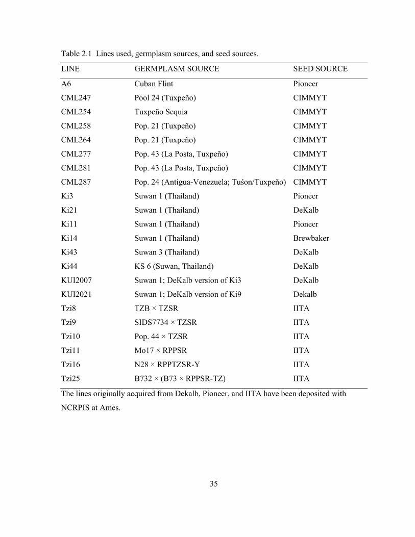
35
Table 2.1 Lines used, germplasm sources, and seed sources.
LINE GERMPLASM SOURCE SEED SOURCE
A6 Cuban Flint Pioneer
CML247 Pool 24 (Tuxpeño) CIMMYT
CML254 Tuxpeño Sequia CIMMYT
CML258 Pop. 21 (Tuxpeño) CIMMYT
CML264 Pop. 21 (Tuxpeño) CIMMYT
CML277 Pop. 43 (La Posta, Tuxpeño) CIMMYT
CML281 Pop. 43 (La Posta, Tuxpeño) CIMMYT
CML287 Pop. 24 (Antigua-Venezuela; Tuśon/Tuxpeño) CIMMYT
Ki3 Suwan 1 (Thailand) Pioneer
Ki21 Suwan 1 (Thailand) DeKalb
Ki11 Suwan 1 (Thailand) Pioneer
Ki14 Suwan 1 (Thailand) Brewbaker
Ki43 Suwan 3 (Thailand) DeKalb
Ki44 KS 6 (Suwan, Thailand) DeKalb
KUI2007 Suwan 1; DeKalb version of Ki3 DeKalb
KUI2021 Suwan 1; DeKalb version of Ki9 Dekalb
Tzi8 TZB × TZSR IITA
Tzi9 SIDS7734 × TZSR IITA
Tzi10 Pop. 44 × TZSR IITA
Tzi11 Mo17 × RPPSR IITA
Tzi16 N28 × RPPTZSR-Y IITA
Tzi25 B732 × (B73 × RPPSR-TZ) IITA
The lines originally acquired from Dekalb, Pioneer, and IITA have been deposited with
NCRPIS at Ames.
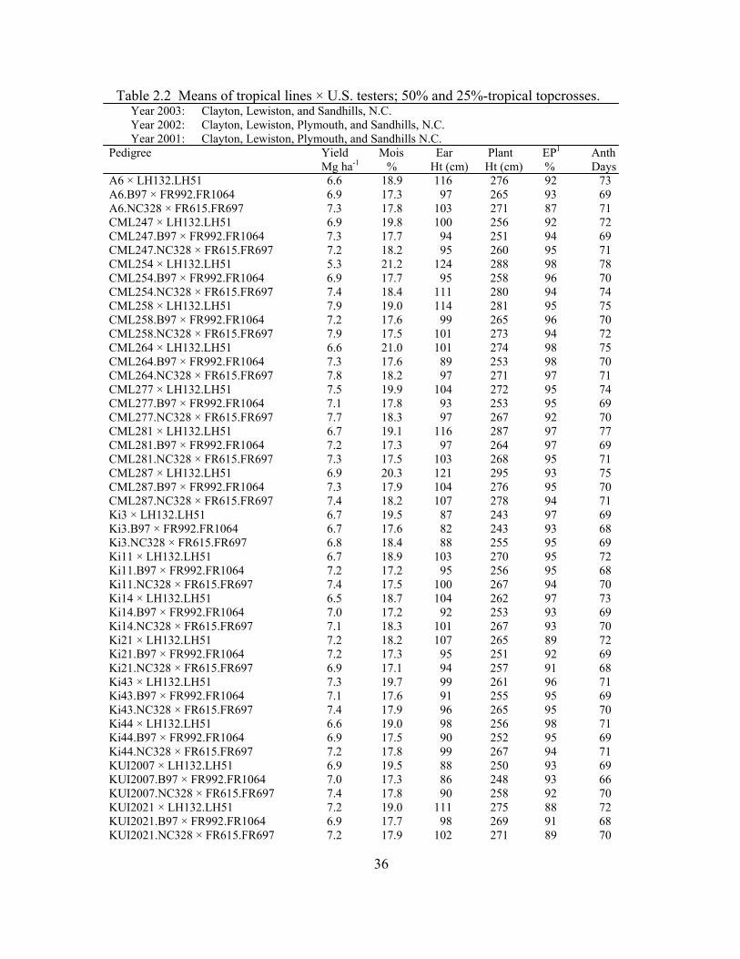
Table 2.2 Means of tropical lines × U.S. testers; 50% and 25%-tropical topcrosses. Year 2003: Clayton, Lewiston, and Sandhills, N.C. Year 2002: Clayton, Lewiston, Plymouth, and Sandhills, N.C. Year 2001: Clayton, Lewiston, Plymouth, and Sandhills N.C. Pedigree Yield Mois Ear Plant EP1 Anth Mg ha-1 % Ht (cm) Ht (cm) % Days A6 × LH132.LH51 6.6 18.9 116 276 92 73 A6.B97 × FR992.FR1064 6.9 17.3 97 265 93 69 A6.NC328 × FR615.FR697 7.3 17.8 103 271 87 71 CML247 × LH132.LH51 6.9 19.8 100 256 92 72 CML247.B97 × FR992.FR1064 7.3 17.7 94 251 94 69 CML247.NC328 × FR615.FR697 7.2 18.2 95 260 95 71 CML254 × LH132.LH51 5.3 21.2 124 288 98 78 CML254.B97 × FR992.FR1064 6.9 17.7 95 258 96 70 CML254.NC328 × FR615.FR697 7.4 18.4 111 280 94 74 CML258 × LH132.LH51 7.9 19.0 114 281 95 75 CML258.B97 × FR992.FR1064 7.2 17.6 99 265 96 70 CML258.NC328 × FR615.FR697 7.9 17.5 101 273 94 72 CML264 × LH132.LH51 6.6 21.0 101 274 98 75 CML264.B97 × FR992.FR1064 7.3 17.6 89 253 98 70 CML264.NC328 × FR615.FR697 7.8 18.2 97 271 97 71 CML277 × LH132.LH51 7.5 19.9 104 272 95 74 CML277.B97 × FR992.FR1064 7.1 17.8 93 253 95 69 CML277.NC328 × FR615.FR697 7.7 18.3 97 267 92 70 CML281 × LH132.LH51 6.7 19.1 116 287 97 77 CML281.B97 × FR992.FR1064 7.2 17.3 97 264 97 69 CML281.NC328 × FR615.FR697 7.3 17.5 103 268 95 71 CML287 × LH132.LH51 6.9 20.3 121 295 93 75 CML287.B97 × FR992.FR1064 7.3 17.9 104 276 95 70 CML287.NC328 × FR615.FR697 7.4 18.2 107 278 94 71 Ki3 × LH132.LH51 6.7 19.5 87 243 97 69 Ki3.B97 × FR992.FR1064 6.7 17.6 82 243 93 68 Ki3.NC328 × FR615.FR697 6.8 18.4 88 255 95 69 Ki11 × LH132.LH51 6.7 18.9 103 270 95 72 Ki11.B97 × FR992.FR1064 7.2 17.2 95 256 95 68 Ki11.NC328 × FR615.FR697 7.4 17.5 100 267 94 70 Ki14 × LH132.LH51 6.5 18.7 104 262 97 73 Ki14.B97 × FR992.FR1064 7.0 17.2 92 253 93 69 Ki14.NC328 × FR615.FR697 7.1 18.3 101 267 93 70 Ki21 × LH132.LH51 7.2 18.2 107 265 89 72 Ki21.B97 × FR992.FR1064 7.2 17.3 95 251 92 69 Ki21.NC328 × FR615.FR697 6.9 17.1 94 257 91 68 Ki43 × LH132.LH51 7.3 19.7 99 261 96 71 Ki43.B97 × FR992.FR1064 7.1 17.6 91 255 95 69 Ki43.NC328 × FR615.FR697 7.4 17.9 96 265 95 70 Ki44 × LH132.LH51 6.6 19.0 98 256 98 71 Ki44.B97 × FR992.FR1064 6.9 17.5 90 252 95 69 Ki44.NC328 × FR615.FR697 7.2 17.8 99 267 94 71 KUI2007 × LH132.LH51 6.9 19.5 88 250 93 69 KUI2007.B97 × FR992.FR1064 7.0 17.3 86 248 93 66 KUI2007.NC328 × FR615.FR697 7.4 17.8 90 258 92 70 KUI2021 × LH132.LH51 7.2 19.0 111 275 88 72 KUI2021.B97 × FR992.FR1064 6.9 17.7 98 269 91 68 KUI2021.NC328 × FR615.FR697 7.2 17.9 102 271 89 70
36
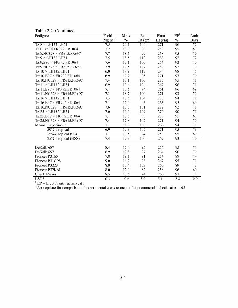
Table 2.2 Continued Pedigree Yield Mois Ear Plant EP1 Anth Mg ha-1 % Ht (cm) Ht (cm) % Days Tzi8 × LH132.LH51 7.5 20.1 104 271 96 72 Tzi8.B97 × FR992.FR1064 7.2 18.3 96 259 95 69 Tzi8.NC328 × FR615.FR697 7.7 18.6 99 268 95 70 Tzi9 × LH132.LH51 7.5 18.5 112 283 92 72 Tzi9.B97 × FR992.FR1064 7.6 17.1 100 264 92 70 Tzi9.NC328 × FR615.FR697 7.9 17.5 107 282 92 70 Tzi10 × LH132.LH51 6.0 18.9 117 286 98 75 Tzi10.B97 × FR992.FR1064 6.9 17.2 98 271 97 70 Tzi10.NC328 × FR615.FR697 7.4 18.1 100 275 95 71 Tzi11 × LH132.LH51 6.9 19.4 104 269 96 71 Tzi11.B97 × FR992.FR1064 7.1 17.6 94 261 96 69 Tzi11.NC328 × FR615.FR697 7.3 18.7 100 271 93 70 Tzi16 × LH132.LH51 7.3 17.6 104 276 94 71 Tzi16.B97 × FR992.FR1064 7.1 17.0 95 263 95 69 Tzi16.NC328 × FR615.FR697 7.6 17.0 101 272 92 71 Tzi25 × LH132.LH51 7.0 19.0 109 270 90 71 Tzi25.B97 × FR992.FR1064 7.1 17.5 93 255 95 69 Tzi25.NC328 × FR615.FR697 7.4 17.8 102 271 94 70 Means: Experiment 7.1 18.3 100 266 94 71 50%-Tropical 6.9 19.3 107 271 95 73 25%-Tropical (SS) 7.1 17.5 94 258 95 69
25%-Tropical (NSS) 7.4 17.9 100 269 93 70 DeKalb 687 8.4 17.4 95 256 95 71 DeKalb 697 8.9 17.8 97 264 90 70 Pioneer P3165 7.8 19.1 91 254 89 74 Pioneer P31G98 9.0 16.7 98 267 95 71 Pioneer P3223 8.9 17.4 103 260 89 73 Pioneer P32K61 8.0 17.0 82 258 96 69 Check Means 8.5 17.6 94 260 92 71 LSD* 0.3 0.6 3.9 5.1 3.8 0.9 1 EP = Erect Plants (at harvest). *Appropriate for comparison of experimental cross to mean of the commercial checks at α = .05
37
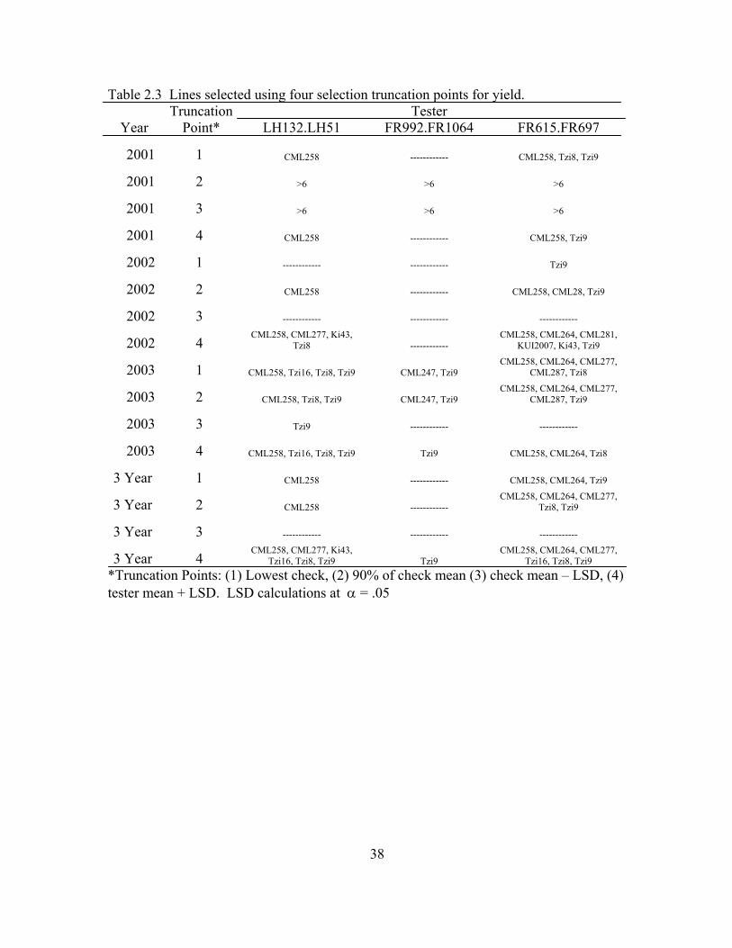
Table 2.3 Lines selected using four selection truncation points for yield.
Year Truncation
Point*
LH132.LH51 Tester
FR992.FR1064 FR615.FR697
2001 1 CML258 ------------ CML258, Tzi8, Tzi9
2001 2 >6 >6 >6
2001 3 >6 >6 >6
2001 4 CML258 ------------ CML258, Tzi9
2002 1 ------------ ------------ Tzi9
2002 2 CML258 ------------ CML258, CML28, Tzi9
2002 3 ------------ ------------ ------------
2002 4 CML258, CML277, Ki43,
Tzi8 ------------ CML258, CML264, CML281,
KUI2007, Ki43, Tzi9
2003 1 CML258, Tzi16, Tzi8, Tzi9 CML247, Tzi9 CML258, CML264, CML277,
CML287, Tzi8
2003 2 CML258, Tzi8, Tzi9 CML247, Tzi9 CML258, CML264, CML277,
CML287, Tzi9
2003 3 Tzi9 ------------ ------------
2003 4 CML258, Tzi16, Tzi8, Tzi9 Tzi9 CML258, CML264, Tzi8
3 Year 1 CML258 ------------ CML258, CML264, Tzi9
3 Year 2 CML258 ------------ CML258, CML264, CML277,
Tzi8, Tzi9
3 Year 3 ------------ ------------ ------------
3 Year 4 CML258, CML277, Ki43,
Tzi16, Tzi8, Tzi9 Tzi9 CML258, CML264, CML277,
Tzi16, Tzi8, Tzi9 *Truncation Points: (1) Lowest check, (2) 90% of check mean (3) check mean – LSD, (4) tester mean + LSD. LSD calculations at α = .05
38
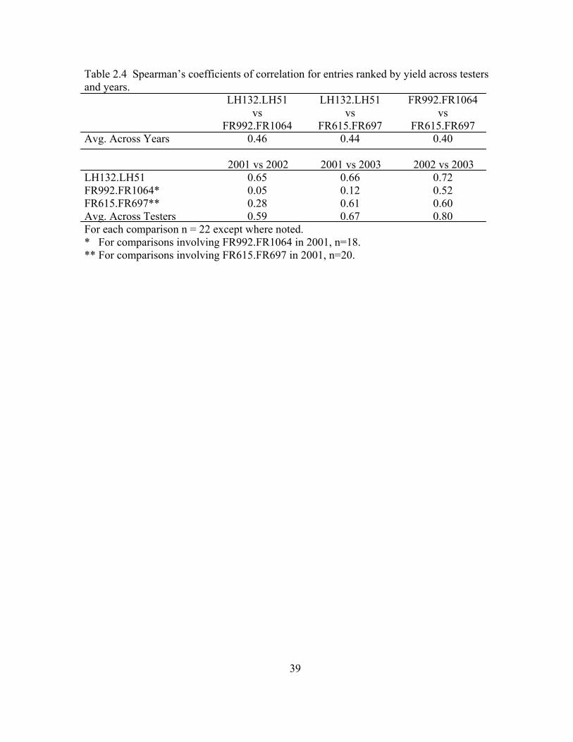
Table 2.4 Spearman’s coefficients of correlation for entries ranked by yield across testers and years. LH132.LH51 LH132.LH51 FR992.FR1064 vs vs vs FR992.FR1064 FR615.FR697 FR615.FR697 Avg. Across Years 0.46 0.44 0.40 2001 vs 2002 2001 vs 2003 2002 vs 2003 LH132.LH51 0.65 0.66 0.72 FR992.FR1064* 0.05 0.12 0.52 FR615.FR697** 0.28 0.61 0.60 Avg. Across Testers 0.59 0.67 0.80 For each comparison n = 22 except where noted. * For comparisons involving FR992.FR1064 in 2001, n=18. ** For comparisons involving FR615.FR697 in 2001, n=20.
39
40
– CHAPTER III –
Selecting Among Available, Elite Exotic Maize Inbreds for Use in Long-Term
Temperate Breeding II
Introduction
The U.S. maize (Zea mays L.) germplasm base is narrow. Thus, ability to adapt to
emerging biotic and abiotic stresses is impaired and there is increased potential for
widespread crop failure as exemplified by the 1970 southern corn leaf blight epidemic
(Horsfall et al., 1972). For years, maize breeders have advocated breeding with tropical
germplasm (Brown, 1953; Brown, 1975; Goodman, 1992, 2004; Lonnquist, 1974; Melhus,
1948; Stuber, 1978; Wellhausen, 1956, 1965), which is the most logical source of added
diversity. However, currently there is very little tropical germplasm represented in U.S.
maize breeding programs (Goodman, 1999).
There are many elite tropical lines which are publicly available from maize breeding
programs in the tropics (Nelson et al., 2006). One reason for the underutilization of this
germplasm resource is the lack of available data on relative line performance. Breeders have
little information on which to base their parental choices. Breeding with exotic germplasm is
difficult and various temperate breeding programs have largly failed in their efforts to use
tropical germplasm because their choice of an exotic collection has been more or less random
(Lonnquist, 1974; Stuber, 1978). Having available information on relative line performance
will likely increase the chances of success with its use.
Various studies have been conducted which provide useful information about tropical
germplasm. Melhus (1948) crossed multiple native Guatemalan collections with U.S.
inbreds and evaluated in them Guatemala. Wellhausen (1956) made exotic intra- and inter-
racial crosses and evaluated them in Mexico. Stuber (1978) screened exotic maize races
from Latin America in North Carolina. The Latin American Maize Project (LAMP)
evaluated over 12,000 tropical exotic accessions in a 5 year cooperative public/private effort
(Salhuana et al., 1991). These screening trials were carried out in the tropics and led to the
identification of many potentially useful tropical accessions (Salhuana et al., 1998). Han et
41
al. (1991), Vasal et al. (1992a; 1992b), and Hede et al. (1999) evaluated tropical inbred maize
lines for combining ability and agronomic performance in tropical environments. Castillo-
Gonzalez and Goodman (1989), Holland and Goodman (1995), and Mickelson et al. (2001)
carried out screening trials of accessions and improved populations in temperate
environments. However, aside from work done by Nelson et al. (2006) there have not been
any published studies that have screened elite tropical inbreds in a temperate environment.
Here we report the results of a screening study, similar to that by done by Nelson et
al. (2006), in which elite tropical inbreds were evaluated in North Carolina and assessed for
use in a temperate breeding program. The objective of this study was to identify elite exotic
maize inbreds that can be used in broadening the U.S. maize germplasm base. The yield data
generated in this study will provide temperate maize breeders with a comprehensive resource
for selecting exotic germplasm. Breeding with exotic germplasm is a costly and time-
consuming endeavor (Goodman, 1992), the success of which is largely determined by choice
of germplasm (Hallauer and Miranda, 1986).
Materials and Methods
Germplasm Selection
Eighty-eight inbred lines, mostly tropical in origin, were chosen for screening. Many
of these lines were identified through unpublished sources, i.e. conference talks, poster
sessions, or word-of-mouth. Each line and its country and breeding program of origin is
listed in Table 3.1. Sixty five of the lines were developed by the International Maize and
Wheat Improvement Center (CIMMYT) in Mexico (Srinivasan, 2001). Eight lines are of
temperate exotic origin, developed at the University of Novi Sad in Serbia. Seven were
developed in Cameroon through joint cooperation of the International Institute of Tropical
Agriculture (IITA) and the Cameroon Institute of Agronomic Research (IRA) (Everett et al.,
1994a, 1994b). Four were developed by Hans Gevers at the Agricultural Research Council’s
Grain Crop Institute in South Africa. Three were developed by IITA in Nigeria. One line
included in the study, an NC296A derivative, is an all-tropical line that was developed at
North Carolina State University but underwent a gametophyte factor conversion attempt at
42
Novi Sad University, Serbia. All lines, except the eight from Serbia, are tropical in origin;
however, for this study all lines will be referred to as ‘exotic’.
The exotic inbreds included in the study were chosen for evaluation for a number of
reasons. First, these lines are exotic from a U.S. perspective, containing many alleles that are
not found in the U.S. maize germplasm base. Second, unlike accessions and unimproved
land races which have been the focus of many studies with exotic germplasm (Castillo-
Gonzalez and Goodman, 1989; Holland and Goodman, 1995; Melhus, 1948; Salhuana et al.,
1998; Stuber, 1978; Wellhausen, 1965), these lines have already seen multiple cycles of
inbreeding and selection. Third, these lines are considered elite in their countries of origin,
showing good yield potential, disease resistance, and overall favorable agronomic
performance. Fourth, they are all publicly available and the seed for most can be obtained
with relative ease.
Yield Trial Evaluation
Yield trial evaluations were carried out from 2001 – 2005. Each exotic line was
initially crossed to a broad-based U.S. tester, LH132 × LH51 (Holden’s Foundation Seeds),
an improved B73 × Mo17 hybrid of Stiff Stalk (SS) × non-Stiff Stalk (NSS) origin. The
resulting 50%-exotic testcrosses were then evaluated in replicated yield trials. Following
each year of testing, the poorest performing lines were eliminated. In general, experimental
entries that were not within one LSD of the check mean were eliminated from the study.
Lines that remained after their first two years of screening then entered two modified three-
way testcrosses, each resulting in a 25%-exotic testcross. In the first of these testcrosses, the
exotic line was crossed to a line of SS origin and then crossed to a NSS × NSS sister-line
hybrid. The SS line used was NC374 and the NSS × NSS sister-line hybrid was FR615 ×
FR697 (Illinois Foundation Seed). In the second of these modified three-way testcrosses,
each exotic line was crossed to a line of NSS origin and then crossed to a SS × SS sister-line
hybrid. The NSS line used was either NC414, NC418, or NC382 and the SS × SS sister-line
hybrid used was FR992 × FR1064 (Illinois Foundation Seed). Therefore, by its third year of
testing, an exotic line was represented in yield trials by three testcrosses, one 50%-exotic
testcross and two 25%-exotic testcrosses. These three testcrosses were then tested together
for the remainder of the study. Because inbreds 326172w, 326633A, and 327609A are of
43
known SS origin, these lines were crossed to FR615 × FR697 for initial screening. Thirteen
commercial hybrid checks were used in the study. These commercial checks represent a
range of maturities grown in North Carolina at the time the study was conducted. All 126
line × tester combinations, the 13 hybrid checks, and the years that they were grown are
listed in Table B.1.
The number of entries included in any single year of testing varied. This is because
newly acquired exotic lines were continually being added to the study and poorly performing
experimental entries were continually being eliminated. Thus, the design was unbalanced
between years because better performing experimental entries were tested for multiple years
while poor performing experimental entries were often eliminated after only one year of
testing. The design was balanced across environments within any given year.
Yield trial evaluations were conducted over five years at five North Carolina
locations, the Central Crops Research Station in Clayton, NC, the Peanut Belt Research
Station in Lewiston / Woodville, NC, the Tidewater Research Station in Plymouth, NC, the
Sandhills Research Station in Jackson Springs, NC, and the Caswell Research Station in
Kinston, NC (Figures B.5 and B.6). These locations were chosen because they represent the
primary maize production regions in North Carolina. Yield trial data were collected at
Clayton and Lewiston all five years. Plots were grown at Plymouth all five years, but yield
trial data from this location was not used in 2003 or 2004 because of hurricane damage.
Plots were grown at Sandhills for four of the five years, 2003 being the exception. Yield trial
data were collected at Kinston in 2004 only. Thus, 18 North Carolina environments were
represented in the study.
Two replications were planted in a double lattice design at all 2001 and 2002
environments and at Clayton, 2004. All other environments had three replications planted in
a triple lattice design. All plots were two rows, 4.88 m in length measured from the center of
the alley, with 1 m alleys, and row spacing of 96.5 cm at all locations except Lewiston where
row spacing was 91.4 cm. Plots were planted with 44 seeds/plot with a target plant density
of 43,000 plants/ha-1 at all locations except Lewiston where target plant density was 45,000
plants/ha-1. Data reported here are limited to yield, moisture percentage at harvest, ear
44
height, plant height, percent erect plants at harvest, and days to anthesis. Days to anthesis
was recorded at Clayton only; all other data were collected at all locations.
Data Analysis
Statistical analysis was done using SAS version 9.1.3 (SAS Institute Inc., 2003).
Data from individual environments was screened for outliers by observing coefficients of
variation and plot residuals. Stand was fitted as a covariate (p < .001) in the analysis of yield
data from Lewiston, 2003, and Sandhills, 2005. Stands at these environments were poor due
to non-genotypic effects, wet cool weather after planting at Lewiston and bird-damage at
Sandhills. Environment means were obtained using each of five statistical models: the
randomized complete block (RCB), lattice, trend, correlated errors (CE), and trend +
correlated errors (T+CE). At four environments, spatial analysis was not an option due to
field constraints or planting errors. As suggested by Brownie et al. (1993), reps were not
included in the trend analysis and only trend effects with p < .01 were included in the trend
or T+CE analysis. Reps were included in the T+CE analysis. Environment means obtained
with each model were compared and a ‘preferred’ analysis was chosen. Comparisons among
analyses were based on F-values for treatment effects, the square root of the average variance
of an entry mean (SAV), spearman rank correlations of treatment means with the RCB, and
the model mean square error (MSE) where applicable (Brownie et al., 1993; Jines et al.,
2006). The RCB served as the default analysis if other analyses failed to be at least 105% as
effective in reducing SAV or if improvements in the other criteria were not present. A single
analysis was chosen for the analysis of each trait across all environments within each year.
This was done to simplify tests for genotype by environment interaction (G×E). Using these
criteria, a preferred analysis was chosen for generating individual entry means within each
environment (Table 3.2).
Entry means across environments were obtained in two ways. First, entry means
from all 18 environments were included in a mixed model analysis using PROC MIXED in
SAS; entries were considered fixed and all other effects were considered random. Through
this mixed analysis, entry means for all 126 experimental entries and 13 checks were
obtained through a single analysis, despite the unbalanced nature of the experiment between
years. However, because of the unequal representation of entries across environments, entry
means are calculated with varying levels of precision. This prevents pairwise comparisons
between entries with a means separation statistic like the least significant difference (LSD).
Second, entry means from individual environments were used to perform across
environment analysis for balanced subsets of entries. These subsets included all entries
grown within any given year, and subsets of entries that were grown together across years.
By splitting the data into balanced subsets, entry means were estimated with equal precision,
thus allowing more appropriate comparisons between entries. For these subsets, a protected
LSD was generated for pair-wise comparisons between experimental entries, comparisons
between an experimental entry and the mean of experimental entries, and comparisons
between an experimental entry and the mean of the commercial checks.
Line × tester interaction for line performance on each of the three testers was
evaluated using the SLICE option with the LSMEANS statement with PROC GLM in SAS.
The SLICE option partitions interaction LSMEANS effects and produces tests of simple
effects (SAS Institute Inc., 2003).
Correlation analysis was done using Spearman’s coefficient of rank correlation for
comparison of line rank on the broad-based, SS, and NSS testers and for comparison of entry
rank across environments.
A “Consistency of Performance” analysis (Ketata et al., 1989) was done by plotting
genotype mean rank against the standard deviation of entry rank across environments.
Within each environment, entries were ranked using PROC RANK in SAS with a TIES =
MEAN statement to assign mean ranking to tied values. Mean entry ranks were obtained
with PROC GLM using an LSMEANS statement. The standard deviations (SE) of entry
ranks were calculated as follows, using residuals outputted from PROC GLM:
SE =1
1
2
−
∑=
n
rn
ii
,
where n is the number of environments and r is the ith residual value (Steel et al., 1997).
45
46
Results and Discussion
Entry Performance
In all analyses except one, F-values for the null hypothesis of no differences between
entries for the given trait were highly significant (p < .01). There were no significant
differences in % erect plants for entries in 2001. This is because there were not any late
season storms in 2001 and all locations had a very high % erect plants.
Entry means are given in Table 3.3 for a subset of the better performing entries. This
subset includes data from 10 environments from 2003 – 2005. Experimental entry values
that did not differ significantly from the mean of the checks are emboldened. Of the 50%-
exotic entries, the CML343 testcross was the highest yielding, followed by the CML274,
CML157Q, CML373, and CML108 testcrosses. These entries also exhibited lodging
resistance, each being within one LSD of the check mean for % erect plants. The CML108
testcross was within one LSD of the check mean for all traits except yield and moisture,
although it was drier than the wettest check, Garst 8288.
Among the 25%-exotic entries, the two CML341and the two CML10 testcrosses were
the four highest yielding. The CML10.NC414 testcross was within one LSD of the check
mean for all traits except moisture.
Data on additional subsets of entries, including individual year means, are given in
Tables B.2 – B.8. Discussion on each of these subsets is also provided in Appendix B.
Line × Tester Interaction
Some lines exhibited significant line × tester interaction. For example, in 2005
CML10 testcrosses with the SS and NSS testers ranked 9th and 10th respectively, yet the
CML10 testcross with the broad-based tester ranked 64th overall. Table 3.4 gives F-values
and significance levels of line × tester interactions. Tests are based on yields expressed as
deviations from the mean yield of all lines on the respective tester. By doing so line × tester
interaction effects due to absolute yield differences between testers are minimized. (Line ×
tester interactions based on actual testcross yields are given in Table B.9.) Based on Table
3.4, only three lines showed significant line × tester interactions, CML10, CML269, and
CML274. Inbred lines CML374, CML103, CML333, CML343, and CML216 showed the
least line × tester interaction.
47
Genotype × Environment Interaction
There was significant G×E for many of the traits in the within-year analysis (Table
B.10). Such interactions may be noteworthy when conducting screening experiments in a
breeding program, particularly when correlations across environments are low. When the
correlation for a single trait is low between two environments, this may suggest that the trait
is being controlled by different genes in different environments (Falconer and Mackay,
1996).
To further address G×E, spearman coefficients of rank correlation between
environments were calculated for experimental entries ranked by trait (Table B.11). These
correlations were higher for highly heritable traits, such as moisture, ear height, and plant
height (Hallauer and Miranda, 1986). Correlations between environments for percent erect
plants were low because this trait is highly affected by environment-specific weather
conditions. Correlations between environments for yield were variable but generally low,
ranging from r = -.02 to r = .67 with a median value of .42.
Stability analysis was performed to further address G×E for yield. Two approaches
were used toward stability analysis, a consistency of performance analysis as described by
Ketata et al. (1989) and an environmental index as proposed by Finlay and Wilkinson (1963).
Neither analysis was performed for 2003 data because there were only two environments in
2003.
Ketata’s consistency of performance analysis establishes a relative measure of
stability by plotting the standard deviation of entry rank across environments against
genotype mean rank. Entries with low standard deviations are considered stable. The “ideal”
genotype will be found near the origin, indicating that it is consistently high-ranking.
Consistency of performance analysis was done on an individual year basis and only
50%-tropical testcrosses (for which data were most complete) were used. Consistency of
performance plots for 2001, 2002, 2004, and 2005 are shown in Figures B.1 – B.4
respectively. By this measure of stability, the CML341 and CML108 testcrosses generally
showed the greatest stability. In all cases, the commercial checks exhibited greater stability
than most of the experimental entries.
48
Methods, results, and discussion on Finlay and Wilkerson’s environmental index are
given in Appendix B.
Tester Correlation
In previous screening trials done at NC State (Nelson et al., 2006), correlation
analysis of line rank on different testers was used to assess the effectiveness of the various
testers in evaluating line performance. For example, if line ranks were highly correlated
across testers, it was concluded that a single tester would have been sufficient for yield trial
screening. However, in the present study, correlation analysis could not be used in this
manner. This is because poorly performing lines were dropped from the experiment in the
early stages of testing. By truncating the distribution in this way, the correlation coefficients
became constrained and unreliable (Levin, 1999). This is especially evident when
considering correlations for testcross yield. Because culling levels in the early stages of
screening were based on yield performance, the distribution for yield was more severely
truncated than the distributions for other traits. This is exemplified in Table B.12 where the
coefficient of correlation for yield ranges from -0.40 to 0.69.
Conclusion
Most of today’s elite U.S. hybrids are derived from a small pool of inbreds that were
developed almost a half-century ago (Goodman, 1992; Smith, 1988; Troyer, 1999). While
maize yields in the U.S. continue to improve (USDA, 2006) and the long-foretold yield
plateau (Wellhausen, 1956) has not yet been reached, there is little evidence that there is a
monopoly on yield genes in the U.S. (Goodman, 1992). The results presented here certainly
indicate that there is yield potential outside the Corn Belt. Within any given year of testing, a
handful of 50%-exotic testcrosses rivaled or beat the check mean in yield performance.
Seven lines stand out across analyses as the better performing lines in the experiment as far
as yield is concerned: CML10, CML108, CML157Q, CML274, CML341, CML343, and
CML373. CML341 testcrosses were the most consistently high-yielding entries. CML108
testcrosses, while not always the highest yielding entries, consistently exhibited superior
performance across all the traits measured.

49
Breeders who are working with tropical-exotic germplasm are faced with a number of
challenges, namely photoperiod sensitivity, disease susceptibility, and weak roots and stocks
(Holland and Goodman, 1995). The magnitude of these challenges can be minimized by
selecting tropical-exotic parents that are more easily adapted. The maize breeding program
at NC State has already begun breeding with many of the lines presented in this study. They
are being used in both exotic × temperate and exotic × exotic breeding crosses and
populations. The lines screened here, in conjunction with lines screened by Nelson et al.
(2006), provide temperate breeders with information on a sizable pool of potentially useful
exotic maize inbred lines. These lines certainly deserve further attention in temperate
breeding efforts.
50
References
Brown, W.L. 1953. Sources of germ plasm for hybrid corn. Corn and Sorghum Res. Conf. Proc. 8:11-16.
Brown, W.L. 1975. A broader germplasm base in corn and sorghum. Corn and Sorghum Res. Conf. Proc. 30:81-89.
Brownie, C., D.T. Bowman, and J.W. Burton. 1993. Estimating spatial variation in analysis of data from yield trials: a comparison of methods. Agronomy Journal 85:1244-1253.
Castillo-Gonzalez, F., and M.M. Goodman. 1989. Agronomic evaluation of Latin-American maize accessions. Crop Science 29:853-861.
Everett, L.A., J.T. Etandu, M. Ndioro, I. Tabi, and S.K. Kim. 1994a. Registration of 19 second-cycle tropical midaltitude maize germplasm lines. Crop Science 34:1419-1420.
Everett, L.A., J.T. Etandu, M. Ndioro, I. Tabi, and S.K. Kim. 1994b. Registration of 18 first-cycle tropical midaltitude maize germplasm lines. Crop Science 34:1422-1422.
Falconer, D.S., and T.F.C. Mackay. 1996. Introduction to quantitative genetics. Fourth ed. Pearson Education Limited, Harlow, England.
Finlay, K.W., and G.N. Wilkinson. 1963. Analysis of adaptation in a plant-breeding programme. Australian Journal of Agricultural Research 14:742-754.
Goodman, M.M. 1992. Choosing and using tropical corn germplasm. Corn and Sorghum Res. Conf. Proc. 47:47-64.
Goodman, M.M. 1999. Broadening the genetic diversity in maize breeding by use of exotic germplasm, p. 139-148, In J. G. Coors and S. Pandey, eds. The genetics and exploitation of heterosis in crops. ASA-CSSA-SSSA, Madison, WI.
Goodman, M.M. 2004. Developing temperate inbreds using tropical maize germplasm: rationale, results, conclusions. Maydica 49:209-219.
Hallauer, A.R., and J.B. Miranda. 1986. Quantitative genetics in maize breeding. Iowa State University Press, Ames, IA.
51
Han, G.C., S.K. Vasal, D.L. Beck, and E. Elias. 1991. Combining ability of inbred lines derived from CIMMYT maize (Zea mays L.) germplasm. Maydica 36:57-64.
Hede, A.R., G. Srinivasan, O. Stolen, and S.K. Vasal. 1999. Identification of heterotic pattern in tropical inbred maize lines using broad-based synthetic testers. Maydica 44:325-331.
Holland, J.B., and M.M. Goodman. 1995. Combining ability of tropical maize accessions with U.S. germplasm. Crop Science 35:767-773.
Horsfall, J.G., G.E. Brandow, W.L. Brown, P.R. Day, W.H. Gabelman, J.B. Hanson, R.F. Holland, A.L. Hooker, P.R. Jennings, V.A. Johnson, D.C. Peters, M.M. Rhoades, G.F. Sprague, S.G. Stephens, J. Tammon, and W.J. Zaumeyer. 1972. Genetic vulnerability of major crops. National Academy of Sciences, Washington, DC.
Jines, M.P., S.J. Szalma, J.B. Holland, and M.M. Goodman. 2006. Spatialpro: A SAS program for automating spatial analysis. (in review).
Ketata, H., S.K. Yau, and M. Nachit. 1989. Relative consistency of performances across environments. Int. Symp. Physiol. Breed. Winter Cereals for Stressed Mediterranean Envir. Montpeiller, July 3-6.
Levin, I.P. 1999. Relating statistics and experimental design: an introduction. Sage Publications, Inc., Thousand Oaks, Calif.
Lonnquist, J.H. 1974. Consideration and experiences with recombinations of exotic and corn belt maize germplasms. Corn and Sorghum Res. Conf. Proc. 29:102-117.
Melhus, L.E. 1948. Exploring the maize germ plasm of the tropics. Corn and Sorghum Res. Conf. Proc. 3:7-19.
Mickelson, H.R., H. Cordova, K.V. Pixley, and M.S. Bjarnason. 2001. Heterotic relationships among nine temperate and subtropical maize populations. Crop Science 41:1012-1020.
Nelson, P.T., M.P. Jines, and M.M. Goodman. 2006. Selecting among available, elite tropical maize inbreds for use in long-term temperate breeding. Maydica 51:(in press).
Salhuana, W., Q. Jones, and R. Sevilla. 1991. The Latin American Maize Project: model for rescue and use of irreplaceable germplasm. Diversity 7:40-42.
52
Salhuana, W., L.M. Pollak, M. Ferrer, O. Paratori, and G. Vivo. 1998. Breeding potential of maize accessions from Argentina, Chile, USA, and Uruguay. Crop Science:866-872.
SAS Institute Inc. 2003. Release 9.1.3. SAS Institute Inc., Cary, NC, USA.
Smith, J.S.C. 1988. Diversity of United States hybrid maize germplasm; Isozymic and chromatographic evidence. Crop Science 28:63-69.
Srinivasan, G. 2001. Maize inbred lines released by CIMMYT [Online] http://148.223.253.105/_private/itdata/CMLsInfo/Maize%20Inbred%20Lines%20Released%20by%20CIMMYT.htm.
Steel, R.G.D., J.H. Torrie, and D.A. Dickey. 1997. Principles and procedures of statistics: a biometrical approach. Third ed. McGraw-Hill, Boston, MA.
Stuber, C.W. 1978. Exotic sources for broadening genetic diversity in corn breeding programs. Corn and Sorghum Res. Conf. Proc. 33:34-47.
Troyer, A.F. 1999. Background of U.S. hybrid corn. Crop Science 39:601-626.
USDA. 2006. Corn: yield by year, US [Online]. Available by USDA http://www.nass.usda.gov/Charts_and_Maps/Field_Crops/cornyld.asp (verified 2/1/06).
Vasal, S.K., G. Srinivasan, G.C. Han, and F.G. C. 1992a. Heterotic patterns of eighty-eight white subtropical CIMMYT maize lines. Maydica 37:319-327.
Vasal, S.K., G. Srinivasan, S. Pandey, H.S. Cordova, G.C. Han, and F. Gonzalez. 1992b. Heterotic Patterns of 92 white tropical CIMMYT maize lines. Maydica 37:259-270.
Wellhausen, E.J. 1956. Improving American corn with exotic germ plasm. The American Seed Trade Association 11:85-96.
Wellhausen, E.J. 1965. Exotic germ plasm for improvement of Corn Belt maize. Corn and Sorghum Res. Conf. Proc. 20:31-45.
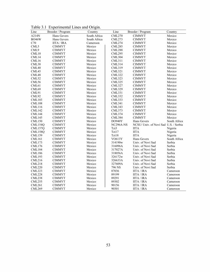
Table 3.1 Experimental Lines and Origin. Line Breeder / Program Country Line Breeder / Program Country A214N Hans Gevers South Africa CML270 CIMMYT Mexico BO46W Hans Gevers South Africa CML273 CIMMYT Mexico C70 IITA / IRA Cameroon CML274 CIMMYT Mexico CML5 CIMMYT Mexico CML285 CIMMYT Mexico CML9 CIMMYT Mexico CML288 CIMMYT Mexico CML10 CIMMYT Mexico CML295 CIMMYT Mexico CML14 CIMMYT Mexico CML304 CIMMYT Mexico CML16 CIMMYT Mexico CML311 CIMMYT Mexico CML38 CIMMYT Mexico CML314 CIMMYT Mexico CML40 CIMMYT Mexico CML319 CIMMYT Mexico CML45 CIMMYT Mexico CML321 CIMMYT Mexico CML48 CIMMYT Mexico CML322 CIMMYT Mexico CML52 CIMMYT Mexico CML323 CIMMYT Mexico CML56 CIMMYT Mexico CML325 CIMMYT Mexico CML61 CIMMYT Mexico CML327 CIMMYT Mexico CML69 CIMMYT Mexico CML329 CIMMYT Mexico CML91 CIMMYT Mexico CML331 CIMMYT Mexico CML92 CIMMYT Mexico CML332 CIMMYT Mexico CML103 CIMMYT Mexico CML333 CIMMYT Mexico CML108 CIMMYT Mexico CML341 CIMMYT Mexico CML116 CIMMYT Mexico CML343 CIMMYT Mexico CML142 CIMMYT Mexico CML373 CIMMYT Mexico CML144 CIMMYT Mexico CML374 CIMMYT Mexico CML145 CIMMYT Mexico CML384 CIMMYT Mexico CML150 CIMMYT Mexico DO940Y Hans Gevers South Africa CML154Q CIMMYT Mexico NC296A-NS NCSU/ Univ. of Novi Sad U.S. / Serbia CML157Q CIMMYT Mexico Tzi3 IITA Nigeria CML158Q CIMMYT Mexico Tzi17 IITA Nigeria CML159 CIMMYT Mexico Tzi18 IITA Nigeria CML161 CIMMYT Mexico VO613Y Hans Gevers South Africa CML173 CIMMYT Mexico 314190w Univ. of Novi Sad Serbia CML176 CIMMYT Mexico 316096A Univ. of Novi Sad Serbia CML184 CIMMYT Mexico 317027A Univ. of Novi Sad Serbia CML186 CIMMYT Mexico 318056A Univ. of Novi Sad Serbia CML193 CIMMYT Mexico 326172w Univ. of Novi Sad Serbia CML216 CIMMYT Mexico 326633A Univ. of Novi Sad Serbia CML218 CIMMYT Mexico 327609A Univ. of Novi Sad Serbia CML220 CIMMYT Mexico 796 NS Univ. of Novi Sad Serbia CML223 CIMMYT Mexico 87036 IITA / IRA Cameroon CML228 CIMMYT Mexico 89199 IITA / IRA Cameroon CML238 CIMMYT Mexico 89291 IITA / IRA Cameroon CML255 CIMMYT Mexico 89302 IITA / IRA Cameroon CML261 CIMMYT Mexico 90156 IITA / IRA Cameroon CML269 CIMMYT Mexico 90301 IITA / IRA Cameroon
53
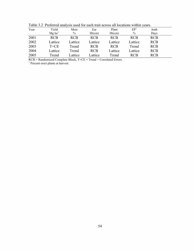
54
Table 3.2 Preferred analysis used for each trait across all locations within years. Year Yield Mois Ear Plant EP1 Anth Mg ha-1 % Ht(cm) Ht(cm) % Days 2001 RCB RCB RCB RCB RCB RCB 2002 Lattice Lattice Lattice Lattice Lattice RCB 2003 T+CE Trend RCB RCB Trend RCB 2004 Lattice Trend RCB Lattice Lattice RCB 2005 Trend Lattice Lattice Trend RCB RCB RCB = Randomized Complete Block, T+CE = Trend + Correlated Errors. 1 Percent erect plants at harvest.
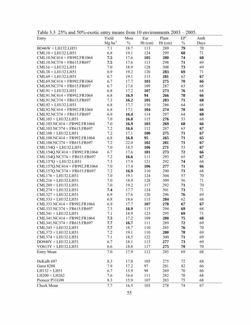
55
Table 3.3 25% and 50%-exotic entry means from 10 environments 2003 – 2005. Entry Yield Mois Ear Plant EP1 Anth Mg ha-1 % Ht (cm) Ht (cm) % Days BO46W × LH132.LH51 7.1 18.7 113 289 79 70 CML10 × LH132.LH51 6.8 19.1 124 299 68 71 CML10.NC414 × FR992.FR1064 7.5 17.6 105 280 74 68 CML10.NC374 × FR615.FR697 7.5 17.6 113 298 71 69 CML16 × LH132.LH51 7.0 18.9 128 308 73 69 CML38 × LH132.LH51 6.9 19.2 120 283 69 71 CML69 × LH132.LH51 6.7 19.1 115 281 62 67 CML69.NC414 × FR992.FR1064 6.7 17.7 103 275 70 66 CML69.NC374 × FR615.FR697 6.7 17.6 109 287 63 68 CML91 × LH132.LH51 6.8 17.2 107 273 76 68 CML91.NC414 × FR992.FR1064 6.8 16.9 94 266 78 66 CML91.NC374 × FR615.FR697 7.3 16.2 105 283 71 68 CML92 × LH132.LH51 6.8 17.7 110 286 64 68 CML92.NC414 × FR992.FR1064 6.8 17.1 104 274 70 66 CML92.NC374 × FR615.FR697 6.9 16.4 114 297 64 68 CML103 × LH132.LH51 7.0 16.8 115 276 53 68 CML103.NC414 × FR992.FR1064 7.0 16.9 103 269 68 66 CML103.NC374 × FR615.FR697 7.2 16.6 112 287 63 67 CML108 × LH132.LH51 7.2 17.1 100 275 71 67 CML108.NC414 × FR992.FR1064 6.8 16.8 95 265 71 65 CML108.NC374 × FR615.FR697 7.2 22.0 102 281 71 67 CML154Q × LH132.LH51 7.0 18.5 106 271 53 67 CML154Q.NC414 × FR992.FR1064 6.7 17.6 101 273 72 66 CML154Q.NC374 × FR615.FR697 7.2 16.6 111 293 65 67 CML157Q × LH132.LH51 7.3 17.9 121 292 74 68 CML157Q.NC414 × FR992.FR1064 7.0 17.4 106 277 71 66 CML157Q.NC374 × FR615.FR697 7.2 16.9 110 290 71 68 CML176 × LH132.LH51 7.0 19.1 124 304 57 70 CML216 × LH132.LH51 7.0 18.9 128 309 56 71 CML269 × LH132.LH51 7.0 19.2 117 292 71 70 CML274 × LH132.LH51 7.4 17.7 124 301 73 71 CML327 × LH132.LH51 6.9 17.6 120 296 76 69 CML333 × LH132.LH51 6.8 18.6 115 284 62 68 CML333.NC414 × FR992.FR1064 6.9 17.7 107 278 67 67 CML333.NC374 × FR615.FR697 7.3 16.9 115 294 69 68 CML341 × LH132.LH51 7.1 18.9 123 295 69 71 CML341.NC414 × FR992.FR1064 7.5 17.2 109 280 75 68 CML341.NC374 × FR615.FR697 7.7 16.7 111 289 72 69 CML343 × LH132.LH51 7.7 18.7 110 285 76 70 CML373 × LH132.LH51 7.2 19.1 110 280 78 69 CML374 × LH132.LH51 7.1 18.5 122 300 71 69 DO940Y × LH132.LH51 6.7 18.1 113 277 73 69 VO613Y × LH132.LH51 6.6 18.8 117 275 70 70 Entry Mean 7.0 17.9 112 285 69 68 DeKalb 697 8.3 17.0 105 275 72 68 Garst 8288 7.9 17.2 97 281 82 66 LH132 × LH51 6.7 15.9 98 269 70 66 LH200 × LH262 7.6 16.6 111 282 70 68 Pioneer P31G98 8.3 15.9 107 283 75 68 Check Mean 7.7 16.5 103 278 74 67
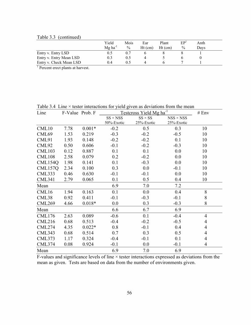
Table 3.3 (continued) Yield Mois Ear Plant EP1 Anth Mg ha-1 % Ht (cm) Ht (cm) % Days Entry v. Entry LSD 0.5 0.7 6 8 8 1 Entry v. Entry Mean LSD 0.3 0.5 4 5 6 0 Entry v. Check Mean LSD 0.4 0.5 4 6 7 1 1 Percent erect plants at harvest.
Table 3.4 Line × tester interactions for yield given as deviations from the mean Line F-Value Prob. F Testcross Yield Mg ha-1 # Env SS × NSS SS × SS NSS × NSS 50%-Exotic 25%-Exotic 25%-Exotic CML10 7.78 0.001* -0.2 0.5 0.3 10 CML69 1.53 0.219 -0.3 -0.2 -0.5 10 CML91 1.93 0.148 -0.2 -0.2 0.1 10 CML92 0.50 0.606 -0.1 -0.2 -0.3 10 CML103 0.12 0.887 0.1 0.1 0.0 10 CML108 2.58 0.079 0.2 -0.2 0.0 10 CML154Q 1.98 0.141 0.1 -0.3 0.0 10 CML157Q 2.34 0.100 0.3 0.0 -0.1 10 CML333 0.46 0.630 -0.1 -0.1 0.0 10 CML341 2.79 0.065 0.1 0.5 0.4 10 Mean 6.9 7.0 7.2 CML16 1.94 0.163 0.1 0.0 0.4 8 CML38 0.92 0.411 -0.1 -0.3 -0.1 8 CML269 4.66 0.018* 0.0 0.3 -0.3 8 Mean 6.6 6.7 6.9 CML176 2.63 0.089 -0.6 0.1 -0.4 4 CML216 0.68 0.513 -0.4 -0.2 -0.5 4 CML274 4.35 0.022* 0.8 -0.1 0.4 4 CML343 0.68 0.514 0.7 0.3 0.5 4 CML373 1.17 0.324 -0.4 -0.1 0.1 4 CML374 0.08 0.924 -0.1 0.0 -0.1 4 Mean 6.9 7.0 6.9 F-values and significance levels of line × tester interactions expressed as deviations from the mean as given. Tests are based on data from the number of environments given.
56
57
– CHAPTER IV –
Gray Leaf Spot Evaluation of Elite Exotic Maize Inbreds
Introduction
Gray leaf spot (GLS) of maize (Zea mays) was first reported by Tehon and Daniels
(1925). It is caused by the fungus Cercospora zeae-maydis and is characterized by long
narrow tan to gray lesions with borders that typically run parallel to the leaf vein (Beckman
and Payne, 1982). Within C. zeae-maydis there are two sibling species and many isolates of
varying levels of aggressiveness (Bair and Ayers, 1986; Carson and Goodman, 2006; Carson
et al., 2002; Dunkle and Carson, 1999).
Gray leaf spot thrives in humid environments that favor slow drying dews and late-
season fogs (Beckman and Payne, 1982). The disease is the most prevalent in the
mountainous regions of Kentucky, Tennessee, Virginia, North Carolina, and South Carolina
(Beckman and Payne, 1983). For many years GLS was found predominantly in these
mountainous regions of the eastern United States and was relatively unimportant in terms of
maize production (Ward et al., 1999). However, since the 1970’s the occurrence of GLS
infection has increased substantially and spread throughout the U.S. corn-belt (Bair and
Ayers, 1986; Beckman and Payne, 1982, 1983; Bubeck et al., 1993; Carson et al., 2002;
Ward et al., 1999). Today GLS is found in maize growing regions from eastern Colorado to
the coasts of North Carolina and Virginia (Carson et al., 2002).
The increased occurrence of GLS is attributed to the coinciding increase in reduced-
tillage and continuous maize cropping systems. Such management practices are conducive to
GLS infestation because C. zeae-maydis overwinters in maize residue that remains on the soil
surface and is easily transmitted to the maize crop the following year. Yield loss caused by
GLS is attributed to decreased photosynthetic leaf area, lodging due to weakened stocks, and
premature plant death in the most serious incidents (Ward et al., 1999). Today GLS is
considered by some to be the most important foliar disease of maize in the U.S. (Carson and
Goodman, 2006; Carson et al., 2002; Gordon et al., 2004).
58
The most efficient means of controlling GLS is through genetic resistance (Carson
and Goodman, 2006; Carson et al., 2002; Graham et al., 1993; Thompson et al., 1987; Ward
et al., 1999). Most of today’s commercial hybrids contain some level of genetic GLS
resistance, but few are highly resistant (Graham et al., 1993; Goodman, unpublished data).
Though resistance can be found in a variety of genetic backgrounds, it most commonly
comes through non-Stiff Stalk (NSS) and tropical sources (Carson and Goodman, 2006;
Carson et al., 2002; Graham et al., 1993; Thompson et al., 1987). Thus, breeders are often
limited in their choice of a Stiff-Stalk (SS) parent in hybrid development if GLS resistance is
of importance. Furthermore, experience at NC State has shown that much of the GLS-
resistant germplasm performs rather poorly with regards to yield and other agronomic
characteristics (Bubeck et al., 1993; Goodman, unpublished data). Thus, there is a need for
additional sources of GLS-resistant germplasm that not only exhibit high yield potential, but
that combine well with NSS germplasm.
Previously, Nelson et al. (2006) and Nelson (Chapter 3 of this thesis) reported on the
agronomic performance of 110 tropical and temperate-exotic inbred lines in testcrosses. The
objective of those studies was to identify exotic sources of maize germplasm that carry
favorable yield and agronomic and traits and can be used in broadening the U.S. maize
germplasm base. Here we report GLS screening results for a similar set of inbred lines, most
of which were included in the aforementioned studies. The primary objective in conducting
this study was to identify tropical sources of GLS resistance. The results of this study, in
conjunction with the results of Nelson et al. (2006) and Nelson (Chapter 3 of this thesis), will
provide temperate maize breeders with a comprehensive resource for selecting tropical
germplasm that is GLS-resistant and exhibits favorable agronomic characteristics.
Materials and Methods
Germplasm Selection
The 102 exotic inbreds screened for GLS resistance were chosen because they are
likely candidates for use in broadening the U.S. maize germplasm base. They have potential
for contributing not only GLS resistance, but favorable yield and other agronomic
characteristics to U.S. maize. Most of the lines were developed by the International Maize
59
and Wheat Improvement Center (CIMMYT) in Mexico (Srinivasan, 2001). Eight were
developed by the International Institute of Tropical Agriculture (IITA) in Nigeria. Seven
were developed in Cameroon through joint cooperation of IITA and the Cameroon Institute
of Agronomic Research (IRA) (Everett et al., 1994a, 1994b). Six were developed at
Kasetsart University in Thailand (Chutkaew et al.). Four are of temperate exotic origin,
developed at the University of Novi Sad in Serbia. Four were developed by Hans Gevers at
the Agricultural Research Council’s Grain Crop Institute in South Africa. One, A6, is a
Cuban flint developed in Cuba by C. G. del Valle (1952). One line, an NC296A derivative,
is an all-tropical line that was developed at North Carolina State University but underwent a
gametophyte factor conversion attempt at Novi Sad University, Serbia. Table 4.1 lists the
breeding institutions and their relative line prefix.
The exotic lines were screened for GLS as inbreds per se and in testcross
combinations using remnant seed from previous yield trial experiments (Nelson et al., 2006,
Chapter 3 of this thesis). Only 53 of the lines were tested in testcrosses because seed from
some of the poorly performing testcroses (from yield trials) had been discarded. Three lines,
Ki44, NC296A-NS, and Tzi11 were not screened as inbreds per se, but were screened in
testcrosses. Testcrosses were made as follows. The exotic line entered a three-way testcross
with a broad based U.S. tester, LH132 × LH51 (Holden’s Foundation Seeds), an improved
B73 × Mo17 hybrid of SS × NSS origin. Because inbreds 326172w, 326633A, and 327609A
are of known SS origin, these lines were crossed to FR615 × FR697 (Illinois Foundation
Seed). Some of the exotic lines were also represented in two modified three-way testcrosses,
each resulting in a 25%-exotic testcross. In the first of these testcrosses, the exotic line was
crossed to a line of SS origin and then crossed to a NSS × NSS sister-line hybrid. The SS
line used was NC374 and the NSS × NSS sister-line hybrid was FR615 × FR697. In the
second of these modified three-way testcrosses, each exotic line was crossed to a line of NSS
origin and then crossed to a SS × SS sister-line hybrid. The NSS line used was either
NC414, NC418, or NC382 and the SS × SS sister-line hybrid used was FR992 × FR1064
(Illinois Foundation Seed).
Inbred and hybrid checks with varying degrees of GLS susceptibility were included in
the study. The GLS susceptible inbred check was B73. Inbred lines NC250, NC258, and
60
NC304 served as the GLS-resistant checks. The GLS susceptible hybrid checks were
Pioneer 3394 and Pioneer 3223. The GLS-resistant hybrid checks used were DeKalb 687,
Pioneer 32W86, and Pioneer 32K61.
Experimental Design
GLS screening trials were grown in the mountain and western piedmont regions of
North Carolina at three locations: Andrews, NC, Laurel Springs, NC, and Salisbury, NC
(Figures B.5 and B.6). These locations are in areas that are prone to GLS development and
the fields used have a history of severe GLS infection. Plots at Salisbury and Andrews were
planted no-till in fields that had GLS-infected residue from the previous season. Plots at
Laurel Springs were planted into conventional tillage all years except one and were
inoculated with C. zeae-maydis infested sorghum seeds each year when plants were at the V6
growth stage.
Inbred per se screening trials were grown at Andrews from 2000-2005, at Laurel
Springs in 2000, 2001, and 2003-2005, and at Salisbury in 2003. Thus, 12 environments
were represented in inbred per se screening. One replication was planted at nine of the
environments, two replications were planted at the other three environments in a randomized
complete block design. Replication between environments was not equal; for example, some
lines were grown in all 12 environments while some were grown in only one. This is
partially because initial GLS screening efforts among these exotic inbreds were focused only
on lines that performed well in yield trials. However, beginning in 2003, GLS screening
among exotic inbreds was expanded and 100 of the 102 exotic inbreds were screened in
2005. The number of environments in which each line was grown is given in Table 4.2.
Testcross screening trials were grown in two environments only, Andrews and Laurel
Springs in 2005. Plots were arranged in a randomized complete block design with two
replications in each environment.
Plots at Laurel Springs and Salisbury were 4.88 m in length measured from the center
of the alley with 1m alleys and 25 seeds planted per plot. Plots at Andrews were 3.05 m in
length measured from the center of the alley with .80 m alleys and ~15 seeds planted per
plot. Row spacing was .91 m at Laurel Springs and .76 m at Salisbury and Andrews. Target
plant density, in plant/ha-1, was 56,000 at Laurel Springs, 67,000 at Salisbury, and 65,000 at
Andrews.
Visual GLS ratings were given on a 1 – 9 scale as described by Bubeck et al. (1993),
1 being fully susceptible and 9 being fully resistant. The first GLS rating at Laurel Springs
was taken when the majority of the plants in the environment were at anthesis. Initial ratings
at Andrews were taken shortly after anthesis. Subsequent GLS ratings at both locations were
taken at about 10 day intervals until the majority of the plants reached senescence. Three to
four ratings were taken at each environment.
Data Analysis
An average GLS rating was obtained for each plot using the area under the disease
progress curve (AUDPC) as initially described by Shaner and Finney (1977) and as given by
Campbell and Madden (1990):
AUDPC = ( )ii
n
i
ii ttyy
−⎟⎠⎞
⎜⎝⎛ +
+
−+∑ 1
11
2
where n is the number of ratings, yi is the ith rating, and ti is the time (days) of the ith rating.
The AUDPC value was standardized to the original 1 – 9 scale by dividing by the total area
of the graph, (tn – t1) (Campbell and Madden, 1990; Fry, 1978).
Statistical analysis was done using SAS version 9.1.3 (SAS Institute Inc., 2003).
Mean GLS ratings within environments (that had multiple replications) and across
environments were obtained using a mixed model; genotypes were considered fixed and all
other effects were considered random. Because the data for inbred per se GLS trials was
unbalanced across environments, mean GLS ratings are estimated with varying levels of
precision as indicated by the standard errors given in Table 4.2. In the analysis of testcross
data from Laurel Springs in 2005, days to anthesis had a significant effect (p = .003) when
included in the model as a covariate. However, because the coefficient of correlation
between means obtained with and without the covariate was very high, r = .98, the covariate
was dropped from the model for the final analysis. A protected LSD was used to assess
differences between testcross entries using Saxton’s (1998) pdmix800 means separation SAS
macro.
61
62
Correlations between inbred per se and testcross GLS ratings were obtained using
Spearman’s coefficient of rank correlation.
Results and Discussion
Entry Performance
In all analyses, F-values for the null hypothesis of no differences in mean GLS rating
between genotypes were highly significant for both inbred per se and testcross trials either
with or without the checks included in the analysis.
Mean GLS ratings for inbreds per se and testcrosses are given in Tables 4.2 and 4.3,
respectively. Experimental entries that performed within the top 10% are emboldened.
Among the inbred lines, CML5, CML14, CML108, and CML145 showed the greatest GLS
resistance. The 12 most resistant inbreds had GLS resistance at or greater than the most
resistant check, NC250, which had a mean GLS rating of 7.3. Among the testcrosses, the
entries with the greatest GLS resistance were the 50%-exotic CML258, CML254, and
CML281 testcrosses and the 25%-exotic CML373.NC374 testcross. There were 30 testcross
entries that were as resistant as or more resistant than the most resistant hybrid check,
Pioneer 32W86, which had a mean GLS rating of 6.9.
Because 50 of the lines were screened both as inbreds per se and as testcrosses, a
correlation analysis was used to address the relationship of GLS resistance in the inbreds per
se and their respective testcrosses. Because inbred per se and testcross GLS screening trials
were done in separate experiments and in different environments, Spearman’s coefficient of
rank correlation, a nonparametric correlation statistic, was used. The correlation between
GLS resistance in inbreds per se and their respective hybrids was relatively high, r = .59.
This suggests that many of the inbreds retained much of their GLS resistance in hybrid
combination.
Gray Leaf Spot and Yield Correlation
Because all of the exotic lines that were tested in GLS screening trials were also
tested in yield trials in earlier studies (Nelson et al., 2006; Chapter 3 of this thesis), a
comparison was done to assess GLS resistance and yield potential. Inbred per se GLS ratings
for each line were plotted against testcross yield performance on the broad based tester,
63
LH132 × LH51. Because yield data are from two separate studies, two plots are given, one
corresponding to yield data from Nelson et al. (2006) (Figure 4.1), and one corresponding to
yield data from Chapter 3 of this thesis (Figure 4.2). Coefficients of correlation, though
negative in both cases, were not significantly different from zero (r = -.08 and r = -.03).
Similar results were seen when testcross GLS scores were plotted against testcross yield
performance (Figures C.1 and C.2).
There are several lines that stand out as having both high GLS resistance and high
yield potential. From Figure 4.1, CML258 was the highest ranked entry for both GLS
resistance and testcross yield performance. CML277 and Tzi16 also had high GLS resistance
and high testcross yield. From Figure 4.2, three lines stand out as having good GLS
resistance and testcross yield, CML108, CML274, and CML343.
The relatively neutral correlation between GLS resistance and testcross yield
performance indicates that GLS resistance among this group of exotic materials is relatively
independent of yield potential. This is good news for breeders who must often sacrifice yield
for disease resistance or vice versa.
Conclusion
Gray leaf spot has become one of the most economically important foliar diseases of
maize. As incidence of GLS increases, so does the need for GLS-resistant germplasm,
especially on the SS side of the pedigree. Here we have identified a group of exotic maize
inbreds, mostly of tropical origin, that carry substantial GLS resistance. Various studies have
shown that many tropical materials combine well with either SS or NSS germplasm (Holland
and Goodman, 1995; Holley and Goodman, 1988; Nelson et al., 2006). Thus, tropical
sources of GLS resistance may be utilized in backcrossing programs with elite SS or NSS
materials without disrupting heterotic patterns. Many of the GLS-resistant lines presented
here also exhibit high yield potential that merits attention beyond a mere backcrossing
program. Such lines are CML108, CML258, CML274, CML277, CML343, and Tzi16.
These lines are valuable to temperate breeders, not only for their high yield potential and
GLS resistance, but also for their contribution of diverse germplasm to the narrowing U.S.
maize germplasm base.
64
References
Bair, W., and J.E. Ayers. 1986. Variability in isolates of Cercospora-zeae-maydis. Phytopathology 76:129-132.
Beckman, P.M., and G.A. Payne. 1982. External growth, penetration, and development of Cercospora-zeae-maydis in corn leaves. Phytopathology 72:810-815.
Beckman, P.M., and G.A. Payne. 1983. Cultural techniques and conditions influencing growth and sporulation of Cercospora-zeae-maydis and lesion development in corn. Phytopathology 73:286-289.
Bubeck, D.M., M.M. Goodman, W.D. Beavis, and D. Grant. 1993. Quantitative trait loci controlling resistance to gray leaf-spot in maize. Crop Science 33:838-847.
Campbell, C.L., and L.V. Madden. 1990. Introduction to plant disease epidemiology. John Wiley & Sons, New York.
Carson, M.L., and M.M. Goodman. 2006. Pathogenicity, agressiveness, and virulence of three species of Cercospora associated with gray leaf spot of maize. Maydica 51:89-92.
Carson, M.L., M.M. Goodman, and S.M. Williamson. 2002. Variation in aggressiveness among isolates of Cercospora from maize as a potential cause of genotype-environment interaction in gray leaf spot trials. Plant Disease 86:1089-1093.
Chutkaew, C., W. Mekdum, and C. Malumpong. Descriptors of Kasetsart University inbred lines [Online] http://www.ku.ac.th/AgrInfo/corn/ (verified 3/06/06).
del Valle, C.G. 1952. La obtención de un hibrido de maiz comercial en Cuba. Estac. Exp. Agron. Santiago de las Vegas (Cuba). Bol. No:69.
Dunkle, L.D., and M.L. Carson. 1999. Genetic variation in Cercospora and the potential impact on selecting for resistance to gray leaf spot in corn. Corn and Sorghum Res. Conf. Proc. 53:334-346.
Everett, L.A., J.T. Etandu, M. Ndioro, I. Tabi, and S.K. Kim. 1994a. Registration of 19 second-cycle tropical midaltitude maize germplasm lines. Crop Science 34:1419-1420.
65
Everett, L.A., J.T. Etandu, M. Ndioro, I. Tabi, and S.K. Kim. 1994b. Registration of 18 first-cycle tropical midaltitude maize germplasm lines. Crop Science 34:1422-1422.
Fry, W.E. 1978. Quantification of general resistance of potato cultivars and fungicide effects for integrated control of potato late blight. Phytopathology 68:1650-1655.
Gordon, S.G., M. Bartsch, I. Matthies, H.O. Gevers, P.E. Lipps, and R.C. Pratt. 2004. Linkage of molecular markers to Cercospora zea-maydis resistance in maize. Crop Science 44:628-636.
Graham, M.J., J.A. Hawk, R.B. Carroll, J.E. Ayers, K.R. Lamkey, and A.R. Hallauer. 1993. Evaluation of Iowa Stiff Stalk synthetic for resistance to gray leaf spot. Plant Disease 77:382-385.
Holland, J.B., and M.M. Goodman. 1995. Combining ability of tropical maize accessions with U.S. germplasm. Crop Science 35:767-773.
Holley, R.N., and M.M. Goodman. 1988. Yield potential of tropical hybrid maize derivatives. Crop Science:213-218.
Nelson, P.T., M.P. Jines, and M.M. Goodman. 2006. Selecting among available, elite tropical maize inbreds for use in long-term temperate breeding. Maydica 51:(in press).
SAS Institute Inc. 2003. Release 9.1.3. SAS Institute Inc., Cary, NC, USA.
Saxton, A.M. 1998. A macro for converting mean separation output to letter groupings in Proc Mixed. 23rd SAS Users Group Intl., SAS Institute, Cary, NC:1243-1246.
Shaner, G., and R.E. Finney. 1977. Effect of nitrogen-fertilization on expression of slow-mildewing resistance in knox wheat. Phytopathology 67:1051-1056.
Srinivasan, G. 2001. Maize inbred lines released by CIMMYT [Online] http://148.223.253.105/_private/itdata/CMLsInfo/Maize%20Inbred%20Lines%20Released%20by%20CIMMYT.htm.
Tehon, L.R., and E. Daniels. 1925. Notes on the parasitic fungi of Illinois. Mycologia 17:240-249.
Thompson, D.L., R.R. Bergquist, G.A. Payne, D.T. Bowman, and M.M. Goodman. 1987. Inheritance of resistance to gray leaf-spot in maize. Crop Science 27:243-246.

66
Ward, J.M.J., E.L. Stromberg, D.C. Nowell, and F.W. Nutter. 1999. Gray leaf spot - a disease of global importance in maize production. Plant Disease 83:884-895.
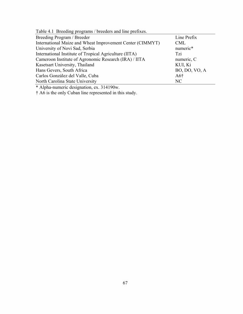
67
Table 4.1 Breeding programs / breeders and line prefixes. Breeding Program / Breeder Line Prefix International Maize and Wheat Improvement Center (CIMMYT) CML University of Novi Sad, Serbia numeric* International Institute of Tropical Agriculture (IITA) Tzi Cameroon Institute of Agronomic Research (IRA) / IITA numeric, C Kasetsart University, Thailand KUI, Ki Hans Gevers, South Africa BO, DO, VO, A Carlos González del Valle, Cuba A6† North Carolina State University NC * Alpha-numeric designation, ex. 314190w. † A6 is the only Cuban line represented in this study.
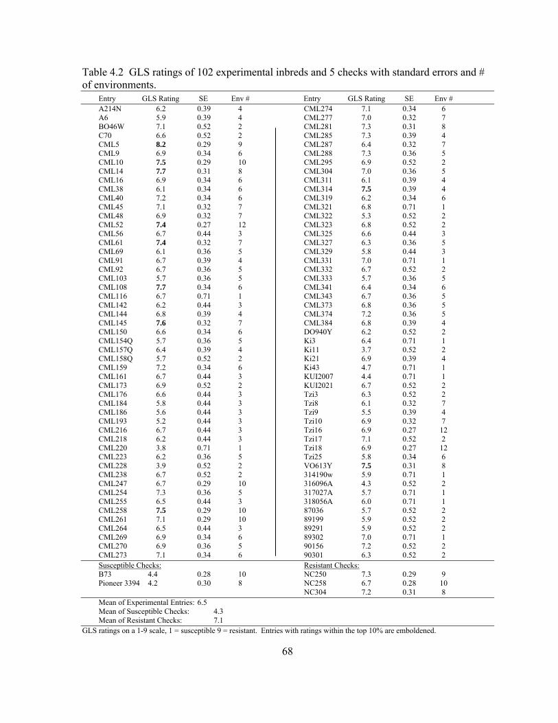
Table 4.2 GLS ratings of 102 experimental inbreds and 5 checks with standard errors and # of environments.
Entry GLS Rating SE Env # Entry GLS Rating SE Env # A214N 6.2 0.39 4 CML274 7.1 0.34 6 A6 5.9 0.39 4 CML277 7.0 0.32 7 BO46W 7.1 0.52 2 CML281 7.3 0.31 8 C70 6.6 0.52 2 CML285 7.3 0.39 4 CML5 8.2 0.29 9 CML287 6.4 0.32 7 CML9 6.9 0.34 6 CML288 7.3 0.36 5 CML10 7.5 0.29 10 CML295 6.9 0.52 2 CML14 7.7 0.31 8 CML304 7.0 0.36 5 CML16 6.9 0.34 6 CML311 6.1 0.39 4 CML38 6.1 0.34 6 CML314 7.5 0.39 4 CML40 7.2 0.34 6 CML319 6.2 0.34 6 CML45 7.1 0.32 7 CML321 6.8 0.71 1 CML48 6.9 0.32 7 CML322 5.3 0.52 2 CML52 7.4 0.27 12 CML323 6.8 0.52 2 CML56 6.7 0.44 3 CML325 6.6 0.44 3 CML61 7.4 0.32 7 CML327 6.3 0.36 5 CML69 6.1 0.36 5 CML329 5.8 0.44 3 CML91 6.7 0.39 4 CML331 7.0 0.71 1 CML92 6.7 0.36 5 CML332 6.7 0.52 2 CML103 5.7 0.36 5 CML333 5.7 0.36 5 CML108 7.7 0.34 6 CML341 6.4 0.34 6 CML116 6.7 0.71 1 CML343 6.7 0.36 5 CML142 6.2 0.44 3 CML373 6.8 0.36 5 CML144 6.8 0.39 4 CML374 7.2 0.36 5 CML145 7.6 0.32 7 CML384 6.8 0.39 4 CML150 6.6 0.34 6 DO940Y 6.2 0.52 2 CML154Q 5.7 0.36 5 Ki3 6.4 0.71 1 CML157Q 6.4 0.39 4 Ki11 3.7 0.52 2 CML158Q 5.7 0.52 2 Ki21 6.9 0.39 4 CML159 7.2 0.34 6 Ki43 4.7 0.71 1 CML161 6.7 0.44 3 KUI2007 4.4 0.71 1 CML173 6.9 0.52 2 KUI2021 6.7 0.52 2 CML176 6.6 0.44 3 Tzi3 6.3 0.52 2 CML184 5.8 0.44 3 Tzi8 6.1 0.32 7 CML186 5.6 0.44 3 Tzi9 5.5 0.39 4 CML193 5.2 0.44 3 Tzi10 6.9 0.32 7 CML216 6.7 0.44 3 Tzi16 6.9 0.27 12 CML218 6.2 0.44 3 Tzi17 7.1 0.52 2 CML220 3.8 0.71 1 Tzi18 6.9 0.27 12 CML223 6.2 0.36 5 Tzi25 5.8 0.34 6 CML228 3.9 0.52 2 VO613Y 7.5 0.31 8 CML238 6.7 0.52 2 314190w 5.9 0.71 1 CML247 6.7 0.29 10 316096A 4.3 0.52 2 CML254 7.3 0.36 5 317027A 5.7 0.71 1 CML255 6.5 0.44 3 318056A 6.0 0.71 1 CML258 7.5 0.29 10 87036 5.7 0.52 2 CML261 7.1 0.29 10 89199 5.9 0.52 2 CML264 6.5 0.44 3 89291 5.9 0.52 2 CML269 6.9 0.34 6 89302 7.0 0.71 1 CML270 6.9 0.36 5 90156 7.2 0.52 2 CML273 7.1 0.34 6 90301 6.3 0.52 2 Susceptible Checks: Resistant Checks: B73 4.4 0.28 10 NC250 7.3 0.29 9
Pioneer 3394 4.2 0.30 8 NC258 6.7 0.28 10 NC304 7.2 0.31 8 Mean of Experimental Entries: 6.5 Mean of Susceptible Checks: 4.3 Mean of Resistant Checks: 7.1
GLS ratings on a 1-9 scale, 1 = susceptible 9 = resistant. Entries with ratings within the top 10% are emboldened.
68
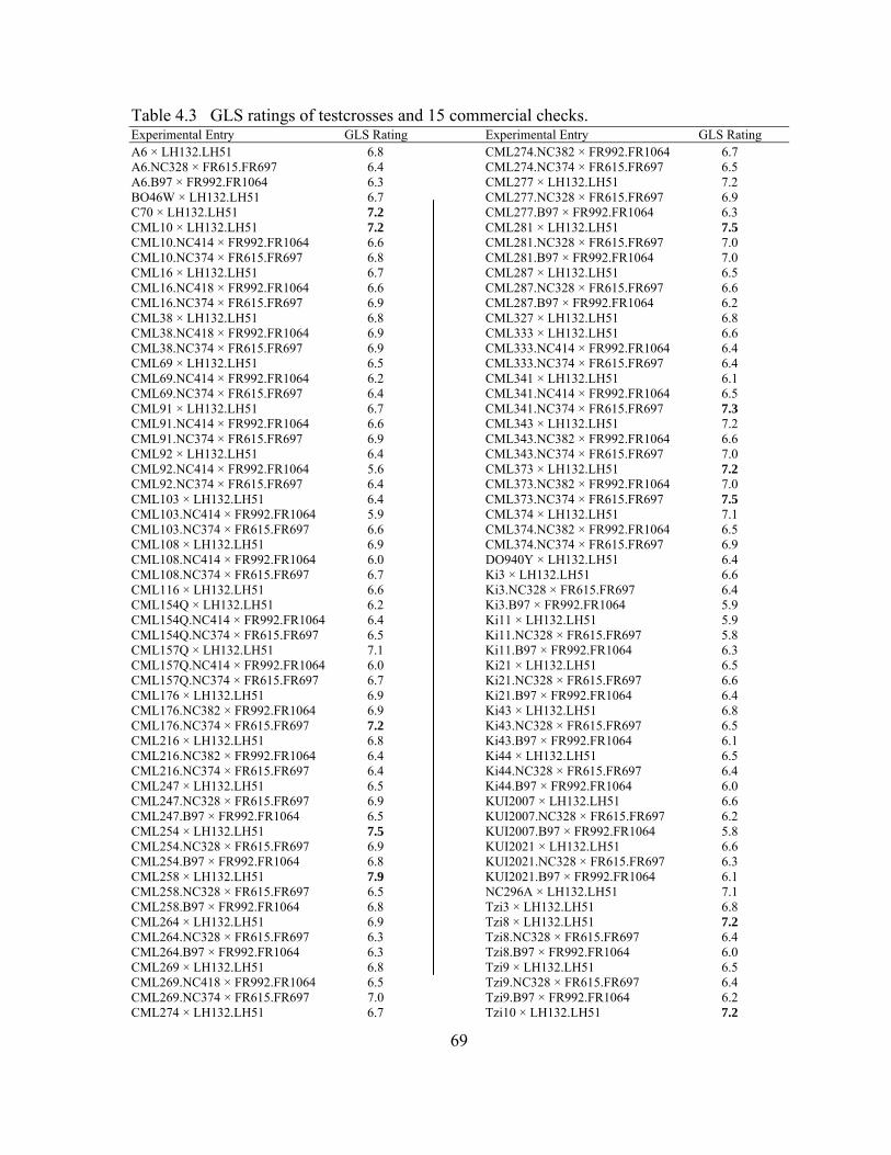
Table 4.3 GLS ratings of testcrosses and 15 commercial checks. Experimental Entry GLS Rating Experimental Entry GLS Rating A6 × LH132.LH51 6.8 CML274.NC382 × FR992.FR1064 6.7 A6.NC328 × FR615.FR697 6.4 CML274.NC374 × FR615.FR697 6.5 A6.B97 × FR992.FR1064 6.3 CML277 × LH132.LH51 7.2 BO46W × LH132.LH51 6.7 CML277.NC328 × FR615.FR697 6.9 C70 × LH132.LH51 7.2 CML277.B97 × FR992.FR1064 6.3 CML10 × LH132.LH51 7.2 CML281 × LH132.LH51 7.5 CML10.NC414 × FR992.FR1064 6.6 CML281.NC328 × FR615.FR697 7.0 CML10.NC374 × FR615.FR697 6.8 CML281.B97 × FR992.FR1064 7.0 CML16 × LH132.LH51 6.7 CML287 × LH132.LH51 6.5 CML16.NC418 × FR992.FR1064 6.6 CML287.NC328 × FR615.FR697 6.6 CML16.NC374 × FR615.FR697 6.9 CML287.B97 × FR992.FR1064 6.2 CML38 × LH132.LH51 6.8 CML327 × LH132.LH51 6.8 CML38.NC418 × FR992.FR1064 6.9 CML333 × LH132.LH51 6.6 CML38.NC374 × FR615.FR697 6.9 CML333.NC414 × FR992.FR1064 6.4 CML69 × LH132.LH51 6.5 CML333.NC374 × FR615.FR697 6.4 CML69.NC414 × FR992.FR1064 6.2 CML341 × LH132.LH51 6.1 CML69.NC374 × FR615.FR697 6.4 CML341.NC414 × FR992.FR1064 6.5 CML91 × LH132.LH51 6.7 CML341.NC374 × FR615.FR697 7.3 CML91.NC414 × FR992.FR1064 6.6 CML343 × LH132.LH51 7.2 CML91.NC374 × FR615.FR697 6.9 CML343.NC382 × FR992.FR1064 6.6 CML92 × LH132.LH51 6.4 CML343.NC374 × FR615.FR697 7.0 CML92.NC414 × FR992.FR1064 5.6 CML373 × LH132.LH51 7.2 CML92.NC374 × FR615.FR697 6.4 CML373.NC382 × FR992.FR1064 7.0 CML103 × LH132.LH51 6.4 CML373.NC374 × FR615.FR697 7.5 CML103.NC414 × FR992.FR1064 5.9 CML374 × LH132.LH51 7.1 CML103.NC374 × FR615.FR697 6.6 CML374.NC382 × FR992.FR1064 6.5 CML108 × LH132.LH51 6.9 CML374.NC374 × FR615.FR697 6.9 CML108.NC414 × FR992.FR1064 6.0 DO940Y × LH132.LH51 6.4 CML108.NC374 × FR615.FR697 6.7 Ki3 × LH132.LH51 6.6 CML116 × LH132.LH51 6.6 Ki3.NC328 × FR615.FR697 6.4 CML154Q × LH132.LH51 6.2 Ki3.B97 × FR992.FR1064 5.9 CML154Q.NC414 × FR992.FR1064 6.4 Ki11 × LH132.LH51 5.9 CML154Q.NC374 × FR615.FR697 6.5 Ki11.NC328 × FR615.FR697 5.8 CML157Q × LH132.LH51 7.1 Ki11.B97 × FR992.FR1064 6.3 CML157Q.NC414 × FR992.FR1064 6.0 Ki21 × LH132.LH51 6.5 CML157Q.NC374 × FR615.FR697 6.7 Ki21.NC328 × FR615.FR697 6.6 CML176 × LH132.LH51 6.9 Ki21.B97 × FR992.FR1064 6.4 CML176.NC382 × FR992.FR1064 6.9 Ki43 × LH132.LH51 6.8 CML176.NC374 × FR615.FR697 7.2 Ki43.NC328 × FR615.FR697 6.5 CML216 × LH132.LH51 6.8 Ki43.B97 × FR992.FR1064 6.1 CML216.NC382 × FR992.FR1064 6.4 Ki44 × LH132.LH51 6.5 CML216.NC374 × FR615.FR697 6.4 Ki44.NC328 × FR615.FR697 6.4 CML247 × LH132.LH51 6.5 Ki44.B97 × FR992.FR1064 6.0 CML247.NC328 × FR615.FR697 6.9 KUI2007 × LH132.LH51 6.6 CML247.B97 × FR992.FR1064 6.5 KUI2007.NC328 × FR615.FR697 6.2 CML254 × LH132.LH51 7.5 KUI2007.B97 × FR992.FR1064 5.8 CML254.NC328 × FR615.FR697 6.9 KUI2021 × LH132.LH51 6.6 CML254.B97 × FR992.FR1064 6.8 KUI2021.NC328 × FR615.FR697 6.3 CML258 × LH132.LH51 7.9 KUI2021.B97 × FR992.FR1064 6.1 CML258.NC328 × FR615.FR697 6.5 NC296A × LH132.LH51 7.1 CML258.B97 × FR992.FR1064 6.8 Tzi3 × LH132.LH51 6.8 CML264 × LH132.LH51 6.9 Tzi8 × LH132.LH51 7.2 CML264.NC328 × FR615.FR697 6.3 Tzi8.NC328 × FR615.FR697 6.4 CML264.B97 × FR992.FR1064 6.3 Tzi8.B97 × FR992.FR1064 6.0 CML269 × LH132.LH51 6.8 Tzi9 × LH132.LH51 6.5 CML269.NC418 × FR992.FR1064 6.5 Tzi9.NC328 × FR615.FR697 6.4 CML269.NC374 × FR615.FR697 7.0 Tzi9.B97 × FR992.FR1064 6.2 CML274 × LH132.LH51 6.7 Tzi10 × LH132.LH51 7.2
69
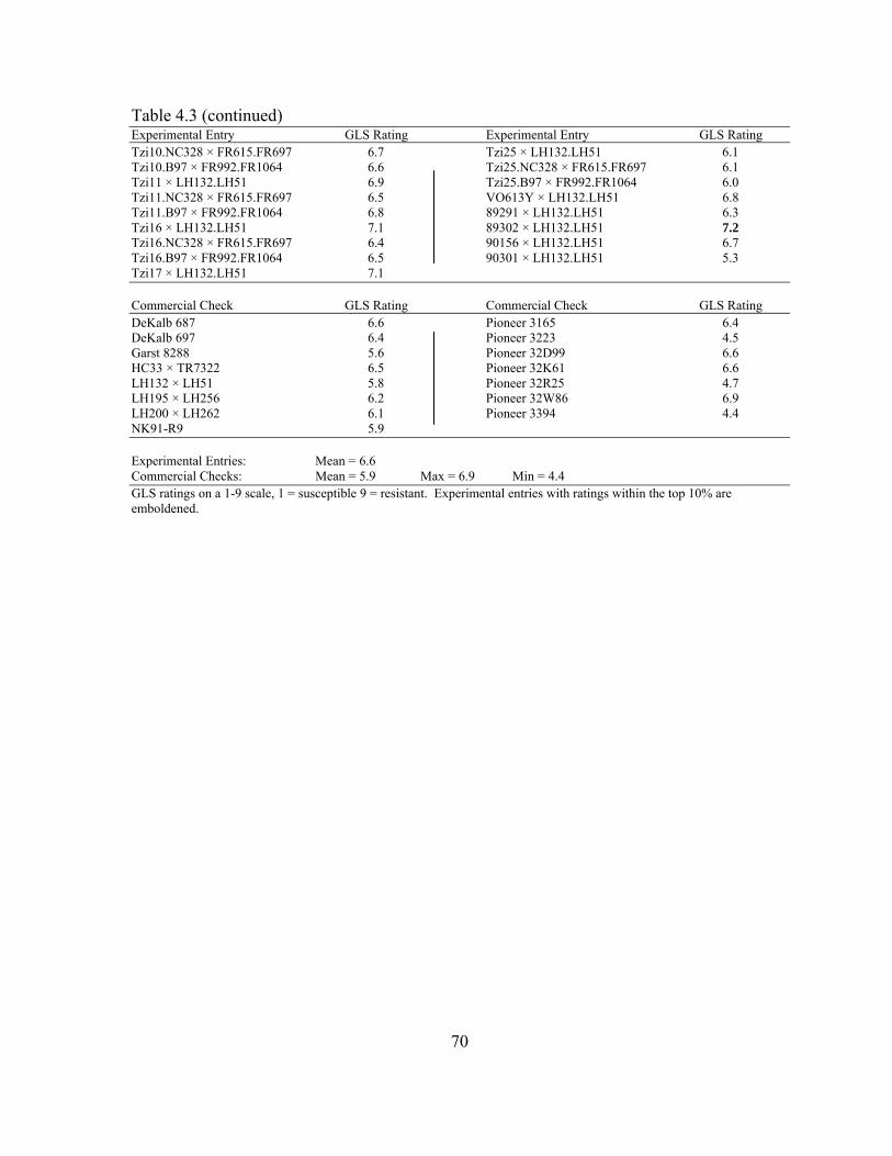
70
Table 4.3 (continued) Experimental Entry GLS Rating Experimental Entry GLS Rating Tzi10.NC328 × FR615.FR697 6.7 Tzi25 × LH132.LH51 6.1 Tzi10.B97 × FR992.FR1064 6.6 Tzi25.NC328 × FR615.FR697 6.1 Tzi11 × LH132.LH51 6.9 Tzi25.B97 × FR992.FR1064 6.0 Tzi11.NC328 × FR615.FR697 6.5 VO613Y × LH132.LH51 6.8 Tzi11.B97 × FR992.FR1064 6.8 89291 × LH132.LH51 6.3 Tzi16 × LH132.LH51 7.1 89302 × LH132.LH51 7.2 Tzi16.NC328 × FR615.FR697 6.4 90156 × LH132.LH51 6.7 Tzi16.B97 × FR992.FR1064 6.5 90301 × LH132.LH51 5.3 Tzi17 × LH132.LH51 7.1 Commercial Check GLS Rating Commercial Check GLS Rating DeKalb 687 6.6 Pioneer 3165 6.4 DeKalb 697 6.4 Pioneer 3223 4.5 Garst 8288 5.6 Pioneer 32D99 6.6 HC33 × TR7322 6.5 Pioneer 32K61 6.6 LH132 × LH51 5.8 Pioneer 32R25 4.7 LH195 × LH256 6.2 Pioneer 32W86 6.9 LH200 × LH262 6.1 Pioneer 3394 4.4 NK91-R9 5.9 Experimental Entries: Mean = 6.6 Commercial Checks: Mean = 5.9 Max = 6.9 Min = 4.4 GLS ratings on a 1-9 scale, 1 = susceptible 9 = resistant. Experimental entries with ratings within the top 10% are emboldened.
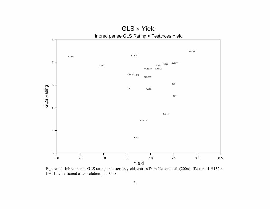
Yield5.0 5.5 6.0 6.5 7.0 7.5 8.0 8.5
GLS
Rat
ing
3
4
5
6
7
8
A6
CML247
CML254
CML258
CML264
CML277
CML281
CML287
KUI11
KUI2007
KUI2021
KUI21
KUI3
KUI43
Tzi10Tzi16
Tzi25
Tzi8
Tzi9
GLS × YieldInbred per se GLS Rating × Testcross Yield
Figure 4.1 Inbred per se GLS ratings × testcross yield, entries from Nelson et al. (2006). Tester = LH132 × LH51. Coefficient of correlation, r = -0.08.
71
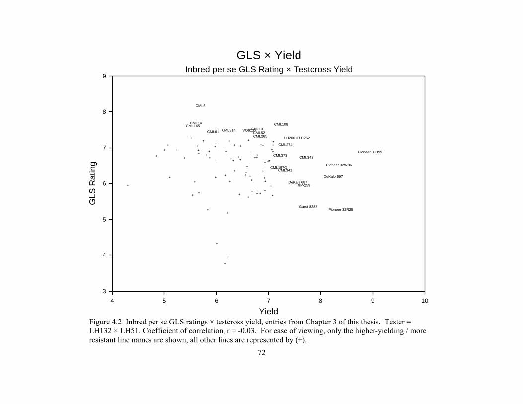
Yield4 5 6 7 8 9 10
GLS
Rat
ing
3
4
5
6
7
8
9
+
+
+
++
+
CML10
+
CML108
+
CML14
+
+
CML145
+
+
CML157Q
+
+
+
+
+
+
+
+
+
+
+
+
+
+
+
+
+++
+ CML274
CML285+
++
+
CML314
+
+
+
+
+
+
+
+
+
+
CML341
CML343CML373
+
+
+
++
+
CML5
CML52
+
CML61
+
+
++
+
DeKalb 687DeKalb 697
+ GP-259
+
+
++
+
Garst 8288
+
+
LH200 × LH262
+
Pioneer 32D99
+
Pioneer 32R25
Pioneer 32W86
+
+
+
VO613Y
GLS × YieldInbred per se GLS Rating × Testcross Yield
Figure 4.2 Inbred per se GLS ratings × testcross yield, entries from Chapter 3 of this thesis. Tester = LH132 × LH51. Coefficient of correlation, r = -0.03. For ease of viewing, only the higher-yielding / more resistant line names are shown, all other lines are represented by (+).
72
73
Appendices
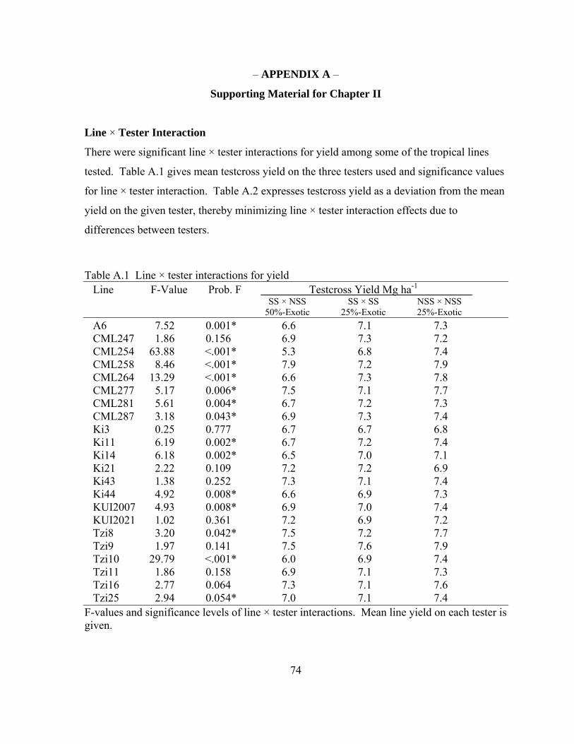
– APPENDIX A –
Supporting Material for Chapter II
Line × Tester Interaction
There were significant line × tester interactions for yield among some of the tropical lines
tested. Table A.1 gives mean testcross yield on the three testers used and significance values
for line × tester interaction. Table A.2 expresses testcross yield as a deviation from the mean
yield on the given tester, thereby minimizing line × tester interaction effects due to
differences between testers.
Table A.1 Line × tester interactions for yield
Line F-Value Prob. F Testcross Yield Mg ha-1 SS × NSS SS × SS NSS × NSS 50%-Exotic 25%-Exotic 25%-Exotic
A6 7.52 0.001* 6.6 7.1 7.3 CML247 1.86 0.156 6.9 7.3 7.2 CML254 63.88 <.001* 5.3 6.8 7.4 CML258 8.46 <.001* 7.9 7.2 7.9 CML264 13.29 <.001* 6.6 7.3 7.8 CML277 5.17 0.006* 7.5 7.1 7.7 CML281 5.61 0.004* 6.7 7.2 7.3 CML287 3.18 0.043* 6.9 7.3 7.4 Ki3 0.25 0.777 6.7 6.7 6.8 Ki11 6.19 0.002* 6.7 7.2 7.4 Ki14 6.18 0.002* 6.5 7.0 7.1 Ki21 2.22 0.109 7.2 7.2 6.9 Ki43 1.38 0.252 7.3 7.1 7.4 Ki44 4.92 0.008* 6.6 6.9 7.3 KUI2007 4.93 0.008* 6.9 7.0 7.4 KUI2021 1.02 0.361 7.2 6.9 7.2 Tzi8 3.20 0.042* 7.5 7.2 7.7 Tzi9 1.97 0.141 7.5 7.6 7.9 Tzi10 29.79 <.001* 6.0 6.9 7.4 Tzi11 1.86 0.158 6.9 7.1 7.3 Tzi16 2.77 0.064 7.3 7.1 7.6 Tzi25 2.94 0.054* 7.0 7.1 7.4
F-values and significance levels of line × tester interactions. Mean line yield on each tester is given.
74
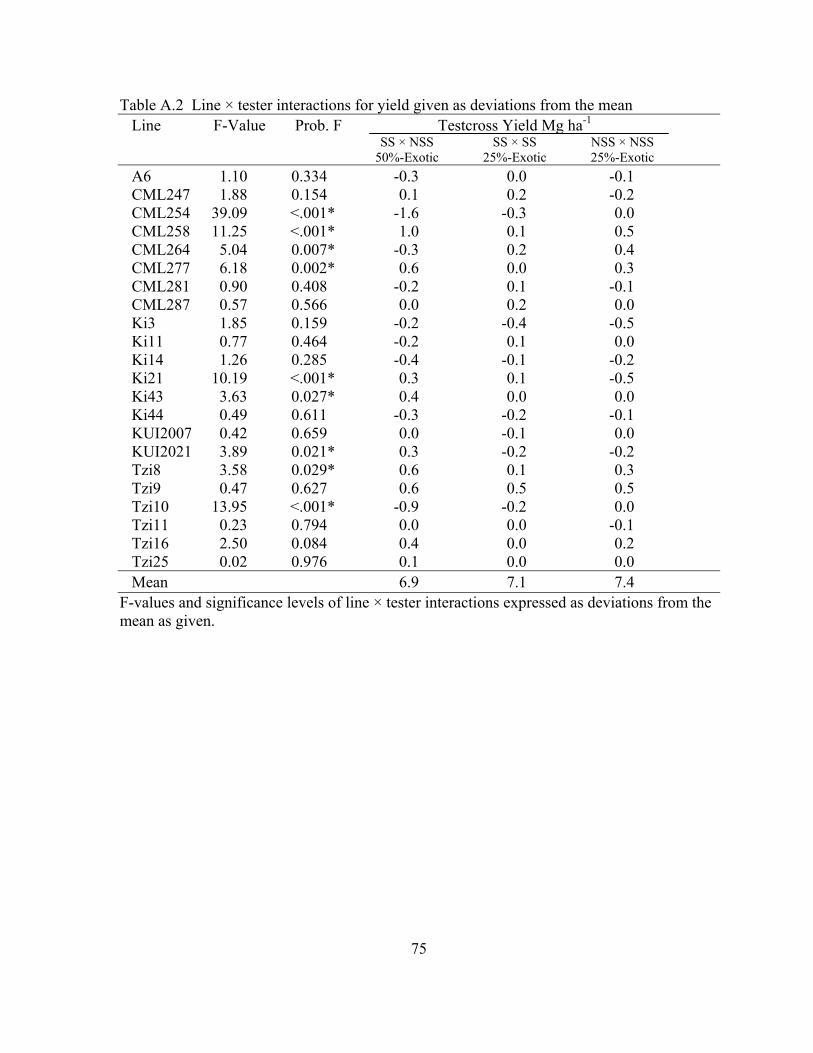
Table A.2 Line × tester interactions for yield given as deviations from the mean Line F-Value Prob. F Testcross Yield Mg ha-1
SS × NSS SS × SS NSS × NSS 50%-Exotic 25%-Exotic 25%-Exotic
A6 1.10 0.334 -0.3 0.0 -0.1 CML247 1.88 0.154 0.1 0.2 -0.2 CML254 39.09 <.001* -1.6 -0.3 0.0 CML258 11.25 <.001* 1.0 0.1 0.5 CML264 5.04 0.007* -0.3 0.2 0.4 CML277 6.18 0.002* 0.6 0.0 0.3 CML281 0.90 0.408 -0.2 0.1 -0.1 CML287 0.57 0.566 0.0 0.2 0.0 Ki3 1.85 0.159 -0.2 -0.4 -0.5 Ki11 0.77 0.464 -0.2 0.1 0.0 Ki14 1.26 0.285 -0.4 -0.1 -0.2 Ki21 10.19 <.001* 0.3 0.1 -0.5 Ki43 3.63 0.027* 0.4 0.0 0.0 Ki44 0.49 0.611 -0.3 -0.2 -0.1 KUI2007 0.42 0.659 0.0 -0.1 0.0 KUI2021 3.89 0.021* 0.3 -0.2 -0.2 Tzi8 3.58 0.029* 0.6 0.1 0.3 Tzi9 0.47 0.627 0.6 0.5 0.5 Tzi10 13.95 <.001* -0.9 -0.2 0.0 Tzi11 0.23 0.794 0.0 0.0 -0.1 Tzi16 2.50 0.084 0.4 0.0 0.2 Tzi25 0.02 0.976 0.1 0.0 0.0 Mean 6.9 7.1 7.4
F-values and significance levels of line × tester interactions expressed as deviations from the mean as given.
75
76
– APPENDIX B –
Supporting Material for Chapter III
Results and Discussion
Subsets of Exotic Entries
In 2001 (Table B.2), the CML341 testcross was the highest yielding experimental
entry, followed by the CML103 and CML108 testcrosses. Of the six highest yielding
experimental entries, five were not significantly different from the check mean for moisture,
and all six flowered within two days of the check mean. The CML108 testcross was better
than or equal to the check mean for all traits except plant height.
In 2002 (Table B.3), the CML341 testcross was again the highest yielding
experimental entry, followed by the CML38, CML269, and CML157Q testcrosses. The
CML16 and CML274 testcrosses, which were new additions to the experiment in 2002, were
also among the highest yielding experimental entries. The CML108 testcross again
performed well overall, being within one LSD of the check mean for all traits.
In 2003 (Table B.4) and thereafter, 25%-exotic testcrosses were included in the study.
Entry means among 25%-exotic entries tend to be superior to those among 50%-exotic
testcrosses because they contain a larger percentage of adapted germplasm. For this reason,
experimental entry performance will be addressed separately for 50%-and 25%-exotic
crosses. Among the 50%-exotic entries, the CML154Q testcross was the highest yielding,
followed by the CML103 and CML373 testcrosses. The CML373 testcross was new to the
study in 2003 and had a higher percentage of erect plants than all other experimental entries,
including the checks. The CML343 testcross, also new in 2003, also had high percentage
erect plants and relatively good yield. The CML108 testcross was again among the top
yielding experimental entries and was within one LSD of the checks for all traits except
moisture. Among the 25%-exotic entries, the CML10.NC374 testcross was the highest
yielding, followed by the CML92.NC374 and CML10.NC414 testcrosses. The
CML341.NC414 and CML154Q.NC414 testcrosses were also among the top yielding
experimental entries.
77
In 2003, plots were planted at three locations, all of which incurred heavy hurricane
damage at the end of the season. Plots at one location were abandoned entirely and the
remaining two locations were harvested despite severe lodging. Because there were fewer
replications and there was substantial plot damage, standard errors and LSDs in 2003 were
larger than in other years. Percent erect plants at harvest for the experimental entries and
checks were low, 45% and 41% respectively. Moistures were also low due to weather-
related harvest delays.
Among the 50%-exotic entries in 2004 (Table B.5), the CML343 testcross was the
highest yielding, followed by the CML373 and CML157Q testcrosses. The CML108
testcross was again among the highest yielding experimental entries and was within one LSD
of the check mean for all traits. Among 25%-exotic entries, the two CML341 testcrosses
were the highest yielding experimental entries, followed by the CML10.NC414 testcross.
The CML341.NC374 testcross was also drier than the check mean.
Among the 50%-exotic entries in 2005 (Table B.6), the CML274 testcross was the
highest yielding followed by the CML343 and 89291 testcrosses. Inbred 89291 was new to
the experiment in 2005. Among the 25%-exotic entries, the CML16.NC374 testcross was the
highest yielding, followed by the CML341.NC374 and CML343.NC374 testcrosses. The
CML274.NC374, CML343.NC382, and both CML10 testcrosses were also among the
highest yielding experimental entries.
Table B.7 gives means for a subset of entries that were tested together from 2002
through 2005, representing data from 14 environments. All experimental entries in this
analysis failed to be within one LSD of the check mean for yield. The CML274 testcross
was the highest yielding experimental entry, followed by the CML341 and CML157Q
testcrosses. The CML108 testcross was also among the highest yielding experimental entry
and was within one LSD of the check mean for all traits except yield. The driest
experimental entry was the CML103 testcross and four experimental entries flowered as
early as the check mean.
Table B.8 gives mean value for all 136 experimental entries and 13 checks taken
across all 18 environments. Because of the unbalanced design across all environments, mean
values are estimated with varying levels of precision as indicated by the standard errors given
78
in the table. Experimental entry mean values that were within the best 10% are emboldened.
Among the 50%-exotic entries, the CML343, 89291, and NC296A testcrosses were the
highest yielding. Among the 25%-exotic entries, the CML343.NC374 and CML341.NC374
testcrosses were the highest yielding.
Stability Analysis Using an Environmental Index
In Finlay and Wilkinson’s (1963) environmental index, entry performance at each
environment is regressed on overall environment mean. The regression coefficient is viewed
as a measure of stability. A regression coefficient of b = 0 indicates that an entry’s
performance does not change over environments, i.e. it is stable. However, this may also
indicate that an entry does not perform to the potential allowed by the environment. A
regression coefficient greater than b = 1 is an indication of instability because such entries
may perform well in optimum conditions only. According to Finlay and Wilkerson, an ideal
genotype will have maximum yield potential in the most favorable environments and also
show stability across environments. Entries with a regression coefficient around b = 1 fit into
this category; they are considered relatively stable across environments and yet adaptable to
changes in the yield potential established by the environment. Environmental index
regression coefficients for each entry are given by year in Tables B.13 – B.16.
References
Finlay, K.W., and G.N. Wilkinson. 1963. Analysis of adaptation in a plant-breeding
programme. Australian Journal of Agricultural Research 14:742-754.
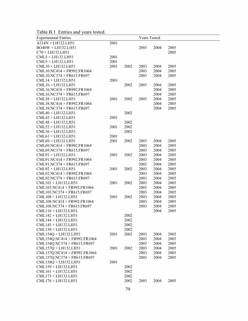
79
Table B.1 Entries and years tested. Experimental Entries Years Tested A214N × LH132.LH51 2001 BO46W × LH132.LH51 2003 2004 2005 C70 × LH132.LH51 2005 CML5 × LH132.LH51 2001 CML9 × LH132.LH51 2001 CML10 × LH132.LH51 2001 2002 2003 2004 2005 CML10.NC414 × FR992.FR1064 2003 2004 2005 CML10.NC374 × FR615.FR697 2003 2004 2005 CML14 × LH132.LH51 2001 CML16 × LH132.LH51 2002 2003 2004 2005 CML16.NC418 × FR992.FR1064 2004 2005 CML16.NC374 × FR615.FR697 2004 2005 CML38 × LH132.LH51 2001 2002 2003 2004 2005 CML38.NC418 × FR992.FR1064 2004 2005 CML38.NC374 × FR615.FR697 2004 2005 CML40 × LH132.LH51 2002 CML45 × LH132.LH51 2001 CML48 × LH132.LH51 2002 CML52 × LH132.LH51 2001 2002 CML56 × LH132.LH51 2002 CML61 × LH132.LH51 2001 CML69 × LH132.LH51 2001 2002 2003 2004 2005 CML69.NC414 × FR992.FR1064 2003 2004 2005 CML69.NC374 × FR615.FR697 2003 2004 2005 CML91 × LH132.LH51 2001 2002 2003 2004 2005 CML91.NC414 × FR992.FR1064 2003 2004 2005 CML91.NC374 × FR615.FR697 2003 2004 2005 CML92 × LH132.LH51 2001 2002 2003 2004 2005 CML92.NC414 × FR992.FR1064 2003 2004 2005 CML92.NC374 × FR615.FR697 2003 2004 2005 CML103 × LH132.LH51 2001 2002 2003 2004 2005 CML103.NC414 × FR992.FR1064 2003 2004 2005 CML103.NC374 × FR615.FR697 2003 2004 2005 CML108 × LH132.LH51 2001 2002 2003 2004 2005 CML108.NC414 × FR992.FR1064 2003 2004 2005 CML108.NC374 × FR615.FR697 2003 2004 2005 CML116 × LH132.LH51 2004 2005 CML142 × LH132.LH51 2002 CML144 × LH132.LH51 2002 CML145 × LH132.LH51 2002 CML150 × LH132.LH51 2002 CML154Q × LH132.LH51 2001 2002 2003 2004 2005 CML154Q.NC414 × FR992.FR1064 2003 2004 2005 CML154Q.NC374 × FR615.FR697 2003 2004 2005 CML157Q × LH132.LH51 2001 2002 2003 2004 2005 CML157Q.NC414 × FR992.FR1064 2003 2004 2005 CML157Q.NC374 × FR615.FR697 2003 2004 2005 CML158Q × LH132.LH51 2001 CML159 × LH132.LH51 2002 CML161 × LH132.LH51 2002 CML173 × LH132.LH51 2002 CML176 × LH132.LH51 2002 2003 2004 2005
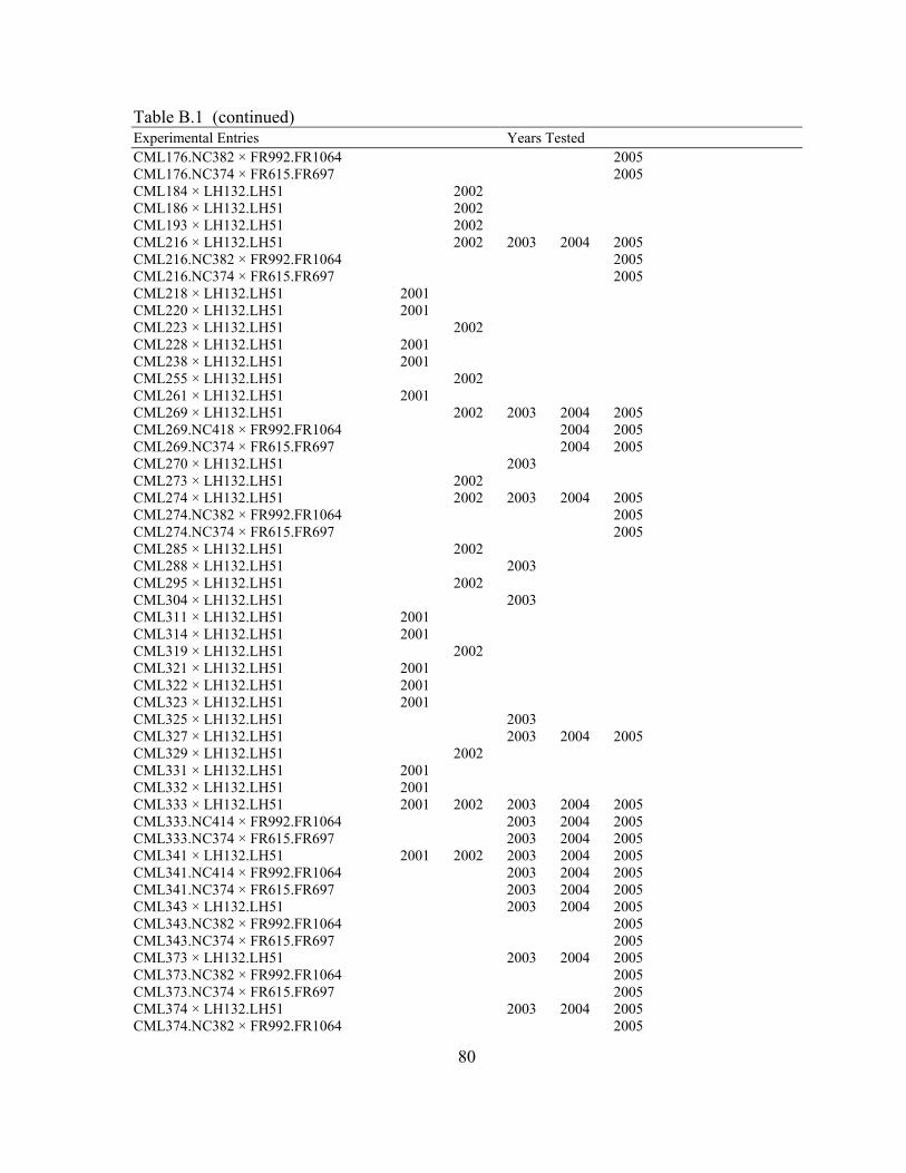
80
Table B.1 (continued) Experimental Entries Years Tested CML176.NC382 × FR992.FR1064 2005 CML176.NC374 × FR615.FR697 2005 CML184 × LH132.LH51 2002 CML186 × LH132.LH51 2002 CML193 × LH132.LH51 2002 CML216 × LH132.LH51 2002 2003 2004 2005 CML216.NC382 × FR992.FR1064 2005 CML216.NC374 × FR615.FR697 2005 CML218 × LH132.LH51 2001 CML220 × LH132.LH51 2001 CML223 × LH132.LH51 2002 CML228 × LH132.LH51 2001 CML238 × LH132.LH51 2001 CML255 × LH132.LH51 2002 CML261 × LH132.LH51 2001 CML269 × LH132.LH51 2002 2003 2004 2005 CML269.NC418 × FR992.FR1064 2004 2005 CML269.NC374 × FR615.FR697 2004 2005 CML270 × LH132.LH51 2003 CML273 × LH132.LH51 2002 CML274 × LH132.LH51 2002 2003 2004 2005 CML274.NC382 × FR992.FR1064 2005 CML274.NC374 × FR615.FR697 2005 CML285 × LH132.LH51 2002 CML288 × LH132.LH51 2003 CML295 × LH132.LH51 2002 CML304 × LH132.LH51 2003 CML311 × LH132.LH51 2001 CML314 × LH132.LH51 2001 CML319 × LH132.LH51 2002 CML321 × LH132.LH51 2001 CML322 × LH132.LH51 2001 CML323 × LH132.LH51 2001 CML325 × LH132.LH51 2003 CML327 × LH132.LH51 2003 2004 2005 CML329 × LH132.LH51 2002 CML331 × LH132.LH51 2001 CML332 × LH132.LH51 2001 CML333 × LH132.LH51 2001 2002 2003 2004 2005 CML333.NC414 × FR992.FR1064 2003 2004 2005 CML333.NC374 × FR615.FR697 2003 2004 2005 CML341 × LH132.LH51 2001 2002 2003 2004 2005 CML341.NC414 × FR992.FR1064 2003 2004 2005 CML341.NC374 × FR615.FR697 2003 2004 2005 CML343 × LH132.LH51 2003 2004 2005 CML343.NC382 × FR992.FR1064 2005 CML343.NC374 × FR615.FR697 2005 CML373 × LH132.LH51 2003 2004 2005 CML373.NC382 × FR992.FR1064 2005 CML373.NC374 × FR615.FR697 2005 CML374 × LH132.LH51 2003 2004 2005 CML374.NC382 × FR992.FR1064 2005
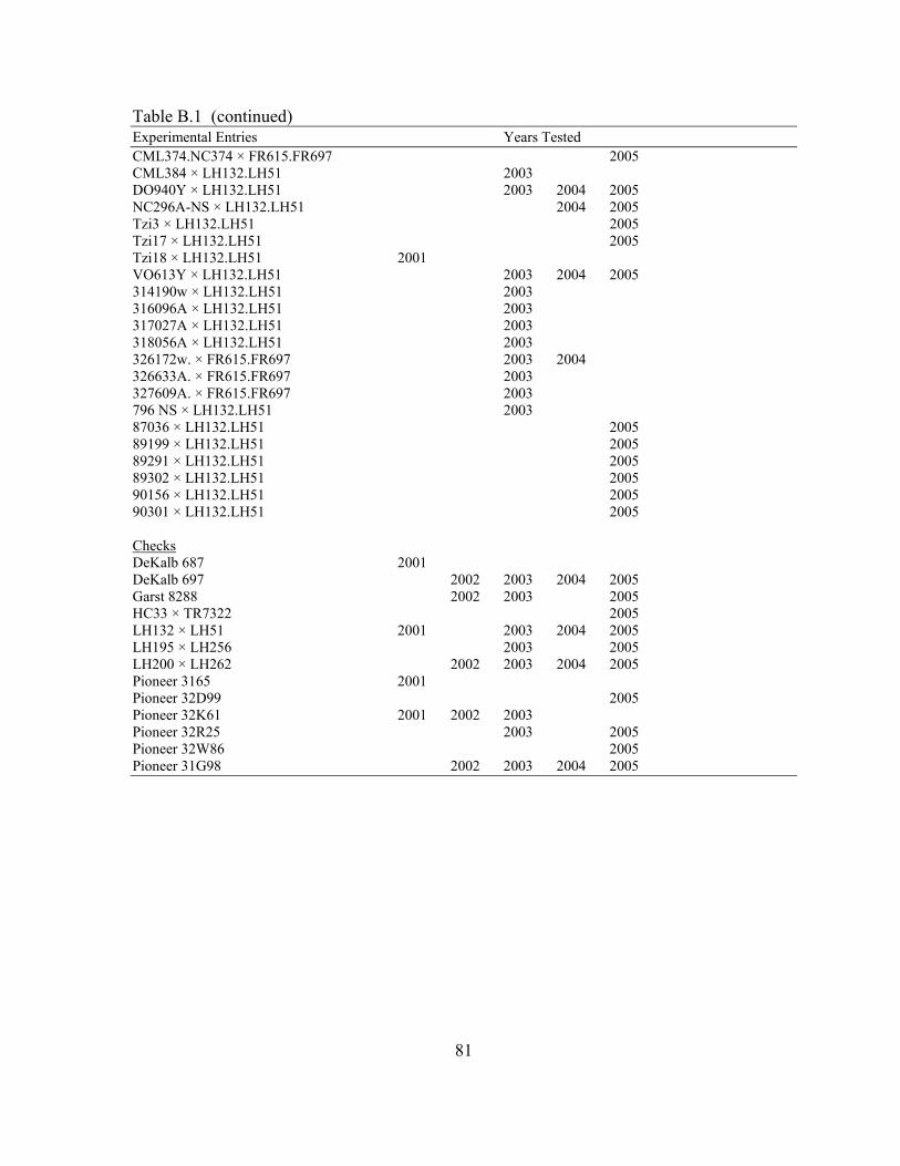
81
Table B.1 (continued) Experimental Entries Years Tested CML374.NC374 × FR615.FR697 2005 CML384 × LH132.LH51 2003 DO940Y × LH132.LH51 2003 2004 2005 NC296A-NS × LH132.LH51 2004 2005 Tzi3 × LH132.LH51 2005 Tzi17 × LH132.LH51 2005 Tzi18 × LH132.LH51 2001 VO613Y × LH132.LH51 2003 2004 2005 314190w × LH132.LH51 2003 316096A × LH132.LH51 2003 317027A × LH132.LH51 2003 318056A × LH132.LH51 2003 326172w. × FR615.FR697 2003 2004 326633A. × FR615.FR697 2003 327609A. × FR615.FR697 2003 796 NS × LH132.LH51 2003 87036 × LH132.LH51 2005 89199 × LH132.LH51 2005 89291 × LH132.LH51 2005 89302 × LH132.LH51 2005 90156 × LH132.LH51 2005 90301 × LH132.LH51 2005 Checks DeKalb 687 2001 DeKalb 697 2002 2003 2004 2005 Garst 8288 2002 2003 2005 HC33 × TR7322 2005 LH132 × LH51 2001 2003 2004 2005 LH195 × LH256 2003 2005 LH200 × LH262 2002 2003 2004 2005 Pioneer 3165 2001 Pioneer 32D99 2005 Pioneer 32K61 2001 2002 2003 Pioneer 32R25 2003 2005 Pioneer 32W86 2005 Pioneer 31G98 2002 2003 2004 2005
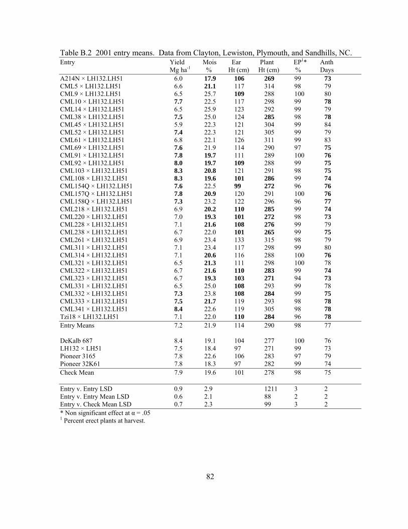
82
Table B.2 2001 entry means. Data from Clayton, Lewiston, Plymouth, and Sandhills, NC. Entry Yield Mois Ear Plant EP1* Anth Mg ha-1 % Ht (cm) Ht (cm) % Days A214N × LH132.LH51 6.0 17.9 106 269 99 73 CML5 × LH132.LH51 6.6 21.1 117 314 98 79 CML9 × LH132.LH51 6.5 25.7 109 288 100 80 CML10 × LH132.LH51 7.7 22.5 117 298 99 78 CML14 × LH132.LH51 6.5 25.9 123 292 99 79 CML38 × LH132.LH51 7.5 25.0 124 285 98 78 CML45 × LH132.LH51 5.9 22.3 121 304 99 84 CML52 × LH132.LH51 7.4 22.3 121 305 99 79 CML61 × LH132.LH51 6.8 22.1 126 311 99 83 CML69 × LH132.LH51 7.6 21.9 114 290 97 75 CML91 × LH132.LH51 7.8 19.7 111 289 100 76 CML92 × LH132.LH51 8.0 19.7 109 288 99 75 CML103 × LH132.LH51 8.3 20.8 121 291 98 75 CML108 × LH132.LH51 8.3 19.6 101 286 99 74 CML154Q × LH132.LH51 7.6 22.5 99 272 96 76 CML157Q × LH132.LH51 7.8 20.9 120 291 100 76 CML158Q × LH132.LH51 7.3 23.2 122 296 96 77 CML218 × LH132.LH51 6.9 20.2 110 285 99 74 CML220 × LH132.LH51 7.0 19.3 101 272 98 73 CML228 × LH132.LH51 7.1 21.6 108 276 99 79 CML238 × LH132.LH51 6.7 22.0 101 265 99 75 CML261 × LH132.LH51 6.9 23.4 133 315 98 79 CML311 × LH132.LH51 7.1 23.4 117 298 99 80 CML314 × LH132.LH51 7.1 20.6 116 288 100 76 CML321 × LH132.LH51 6.5 21.3 111 298 100 78 CML322 × LH132.LH51 6.7 21.6 110 283 99 74 CML323 × LH132.LH51 6.7 19.3 103 271 94 73 CML331 × LH132.LH51 6.5 25.0 108 293 99 78 CML332 × LH132.LH51 7.3 23.8 108 284 99 75 CML333 × LH132.LH51 7.5 21.7 119 293 98 78 CML341 × LH132.LH51 8.4 22.6 119 305 98 78 Tzi18 × LH132.LH51 7.1 22.0 110 284 96 78 Entry Means 7.2 21.9 114 290 98 77 DeKalb 687 8.4 19.1 104 277 100 76 LH132 × LH51 7.5 18.4 97 271 99 73 Pioneer 3165 7.8 22.6 106 283 97 79 Pioneer 32K61 7.8 18.3 97 282 99 74 Check Mean 7.9 19.6 101 278 98 75 Entry v. Entry LSD 0.9 2.9 1211 3 2 Entry v. Entry Mean LSD 0.6 2.1 88 2 2 Entry v. Check Mean LSD 0.7 2.3 99 3 2 * Non significant effect at α = .05 1 Percent erect plants at harvest.
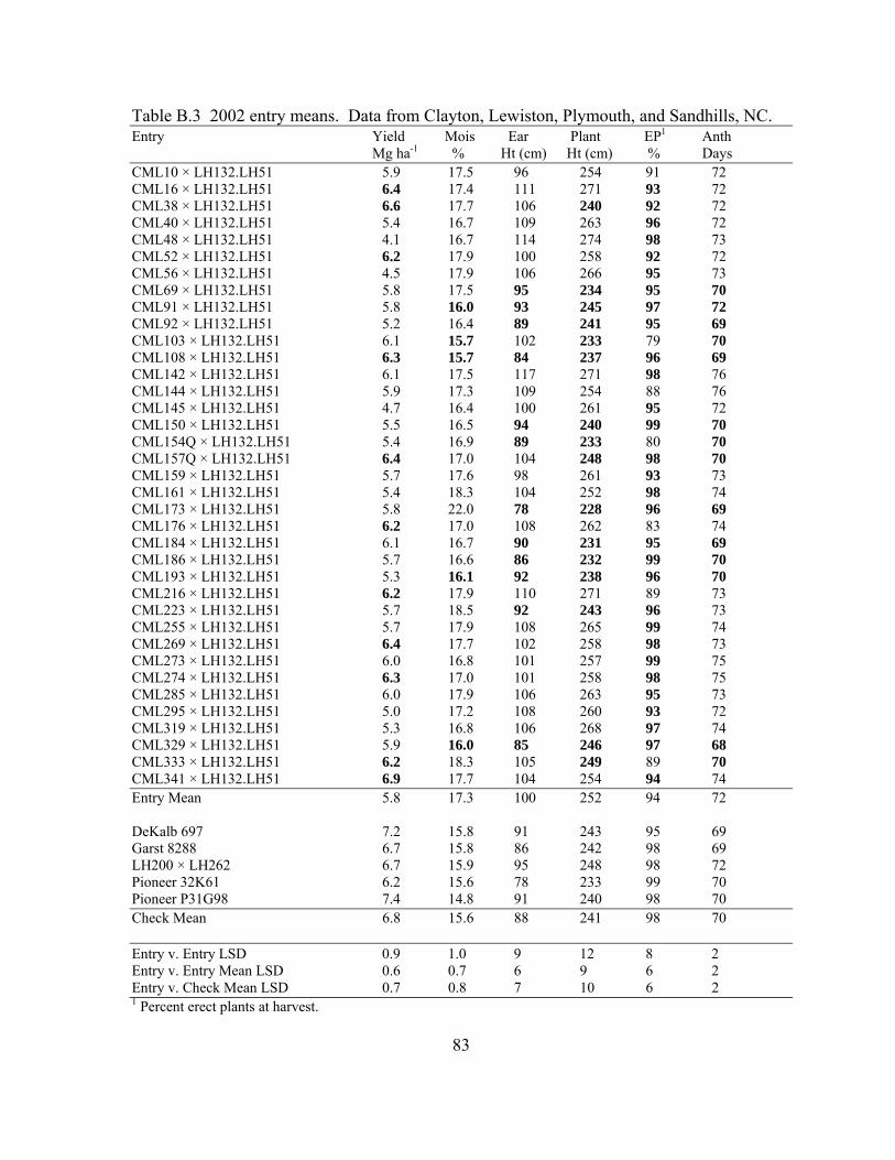
83
Table B.3 2002 entry means. Data from Clayton, Lewiston, Plymouth, and Sandhills, NC. Entry Yield Mois Ear Plant EP1 Anth Mg ha-1 % Ht (cm) Ht (cm) % Days CML10 × LH132.LH51 5.9 17.5 96 254 91 72 CML16 × LH132.LH51 6.4 17.4 111 271 93 72 CML38 × LH132.LH51 6.6 17.7 106 240 92 72 CML40 × LH132.LH51 5.4 16.7 109 263 96 72 CML48 × LH132.LH51 4.1 16.7 114 274 98 73 CML52 × LH132.LH51 6.2 17.9 100 258 92 72 CML56 × LH132.LH51 4.5 17.9 106 266 95 73 CML69 × LH132.LH51 5.8 17.5 95 234 95 70 CML91 × LH132.LH51 5.8 16.0 93 245 97 72 CML92 × LH132.LH51 5.2 16.4 89 241 95 69 CML103 × LH132.LH51 6.1 15.7 102 233 79 70 CML108 × LH132.LH51 6.3 15.7 84 237 96 69 CML142 × LH132.LH51 6.1 17.5 117 271 98 76 CML144 × LH132.LH51 5.9 17.3 109 254 88 76 CML145 × LH132.LH51 4.7 16.4 100 261 95 72 CML150 × LH132.LH51 5.5 16.5 94 240 99 70 CML154Q × LH132.LH51 5.4 16.9 89 233 80 70 CML157Q × LH132.LH51 6.4 17.0 104 248 98 70 CML159 × LH132.LH51 5.7 17.6 98 261 93 73 CML161 × LH132.LH51 5.4 18.3 104 252 98 74 CML173 × LH132.LH51 5.8 22.0 78 228 96 69 CML176 × LH132.LH51 6.2 17.0 108 262 83 74 CML184 × LH132.LH51 6.1 16.7 90 231 95 69 CML186 × LH132.LH51 5.7 16.6 86 232 99 70 CML193 × LH132.LH51 5.3 16.1 92 238 96 70 CML216 × LH132.LH51 6.2 17.9 110 271 89 73 CML223 × LH132.LH51 5.7 18.5 92 243 96 73 CML255 × LH132.LH51 5.7 17.9 108 265 99 74 CML269 × LH132.LH51 6.4 17.7 102 258 98 73 CML273 × LH132.LH51 6.0 16.8 101 257 99 75 CML274 × LH132.LH51 6.3 17.0 101 258 98 75 CML285 × LH132.LH51 6.0 17.9 106 263 95 73 CML295 × LH132.LH51 5.0 17.2 108 260 93 72 CML319 × LH132.LH51 5.3 16.8 106 268 97 74 CML329 × LH132.LH51 5.9 16.0 85 246 97 68 CML333 × LH132.LH51 6.2 18.3 105 249 89 70 CML341 × LH132.LH51 6.9 17.7 104 254 94 74 Entry Mean 5.8 17.3 100 252 94 72 DeKalb 697 7.2 15.8 91 243 95 69 Garst 8288 6.7 15.8 86 242 98 69 LH200 × LH262 6.7 15.9 95 248 98 72 Pioneer 32K61 6.2 15.6 78 233 99 70 Pioneer P31G98 7.4 14.8 91 240 98 70 Check Mean 6.8 15.6 88 241 98 70 Entry v. Entry LSD 0.9 1.0 9 12 8 2 Entry v. Entry Mean LSD 0.6 0.7 6 9 6 2 Entry v. Check Mean LSD 0.7 0.8 7 10 6 2 1 Percent erect plants at harvest.
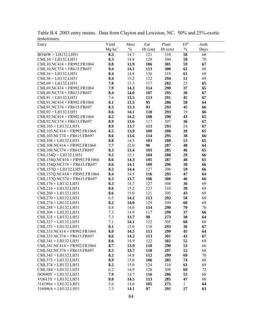
84
Table B.4 2003 entry means. Data from Clayton and Lewiston, NC. 50% and 25%-exotic testcrosses. Entry Yield Mois Ear Plant EP1 Anth Mg ha-1 % Ht (cm) Ht (cm) % Days BO46W × LH132.LH51 8.3 14.7 121 310 58 68 CML10 × LH132.LH51 8.3 14.8 128 304 59 70 CML10.NC414 × FR992.FR1064 8.8 13.9 106 301 59 67 CML10.NC374 × FR615.FR697 9.4 14.1 113 300 62 68 CML16 × LH132.LH51 8.4 14.8 136 319 61 68 CML38 × LH132.LH51 8.4 15.2 122 294 51 69 CML69 × LH132.LH51 7.8 15.3 117 282 23 65 CML69.NC414 × FR992.FR1064 7.9 14.3 114 290 37 65 CML69.NC374 × FR615.FR697 8.4 14.0 107 295 30 67 CML91 × LH132.LH51 7.4 13.5 113 291 45 67 CML91.NC414 × FR992.FR1064 8.1 13.5 95 286 58 64 CML91.NC374 × FR615.FR697 8.3 13.3 93 293 45 66 CML92 × LH132.LH51 8.6 14.1 110 293 19 66 CML92.NC414 × FR992.FR1064 8.2 14.2 108 290 43 65 CML92.NC374 × FR615.FR697 8.9 13.6 117 307 36 67 CML103 × LH132.LH51 8.9 13.7 113 293 24 67 CML103.NC414 × FR992.FR1064 8.5 13.9 109 288 39 65 CML103.NC374 × FR615.FR697 8.6 13.6 114 295 38 66 CML108 × LH132.LH51 8.8 14.5 103 288 53 65 CML108.NC414 × FR992.FR1064 7.7 22.0 96 287 48 64 CML108.NC374 × FR615.FR697 8.3 13.4 103 285 46 65 CML154Q × LH132.LH51 9.2 15.1 104 288 29 66 CML154Q.NC414 × FR992.FR1064 8.6 14.3 105 287 48 65 CML154Q.NC374 × FR615.FR697 8.6 14.1 109 296 38 66 CML157Q × LH132.LH51 8.2 14.4 127 306 59 66 CML157Q.NC414 × FR992.FR1064 8.4 14.5 116 295 47 64 CML157Q.NC374 × FR615.FR697 8.3 13.7 106 300 46 66 CML176 × LH132.LH51 8.3 14.7 127 308 36 69 CML216 × LH132.LH51 8.6 15.2 123 310 38 69 CML269 × LH132.LH51 8.6 15.0 121 305 43 69 CML270 × LH132.LH51 6.5 14.2 113 292 58 68 CML274 × LH132.LH51 8.2 14.0 129 309 60 69 CML288 × LH132.LH51 6.8 14.6 114 290 70 70 CML304 × LH132.LH51 7.3 14.9 117 299 37 66 CML325 × LH132.LH51 7.3 13.7 98 273 38 64 CML327 × LH132.LH51 7.1 14.1 122 305 68 68 CML333 × LH132.LH51 8.1 15.0 118 293 36 67 CML333.NC414 × FR992.FR1064 8.0 14.5 113 299 45 64 CML333.NC374 × FR615.FR697 8.6 14.2 113 301 42 67 CML341 × LH132.LH51 8.6 14.9 122 302 52 69 CML341.NC414 × FR992.FR1064 8.7 13.9 110 298 53 66 CML341.NC374 × FR615.FR697 8.5 13.7 110 297 52 68 CML343 × LH132.LH51 8.2 14.8 112 299 69 70 CML373 × LH132.LH51 8.9 15.0 106 285 74 68 CML374 × LH132.LH51 8.2 15.0 124 310 61 69 CML384 × LH132.LH51 6.2 14.9 128 308 69 72 DO940Y × LH132.LH51 7.9 14.7 116 286 53 68 VO613Y × LH132.LH51 8.0 14.5 113 285 47 68 314190w × LH132.LH51 5.6 14.6 105 275 1 64 316096A × LH132.LH51 7.3 14.1 97 291 27 63
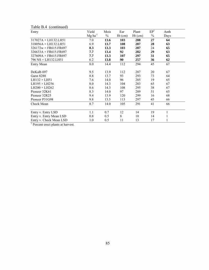
85
Table B.4 (continued) Entry Yield Mois Ear Plant EP1 Anth Mg ha-1 % Ht (cm) Ht (cm) % Days 317027A × LH132.LH51 7.0 13.6 103 288 27 64 318056A × LH132.LH51 6.9 13.7 108 287 28 63 326172w × FR615.FR697 8.3 13.3 103 287 24 65 326633A × FR615.FR697 7.7 13.4 92 282 29 63 327609A × FR615.FR697 7.7 13.3 107 297 31 65 796 NS × LH132.LH51 6.2 13.8 90 257 36 62 Entry Mean 8.0 14.4 112 294 45 67 DeKalb 697 9.5 13.9 112 287 20 67 Garst 8288 8.8 13.7 93 293 73 64 LH132 × LH51 7.6 14.0 96 285 19 65 LH195 × LH256 8.0 14.3 104 283 65 67 LH200 × LH262 8.6 14.3 108 295 38 67 Pioneer 32K61 8.3 14.0 97 289 51 65 Pioneer 32R25 9.4 13.9 120 299 16 68 Pioneer P31G98 9.8 13.5 113 297 45 66 Check Mean 8.7 14.0 105 291 41 66 Entry v. Entry LSD 1.1 0.7 12 14 19 1 Entry v. Entry Mean LSD 0.8 0.5 8 10 14 1 Entry v. Check Mean LSD 1.0 0.5 11 13 17 1 1 Percent erect plants at harvest.
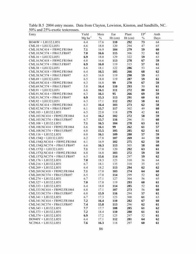
86
Table B.5 2004 entry means. Data from Clayton, Lewiston, Kinston, and Sandhills, NC. 50% and 25%-exotic testcrosses. Entry Yield Mois Ear Plant EP1 Anth Mg ha-1 % Ht (cm) Ht (cm) % Days BO46W × LH132.LH51 6.4 17.6 110 292 73 64 CML10 × LH132.LH51 6.6 18.0 120 294 47 65 CML10.NC414 × FR992.FR1064 7.1 16.9 104 279 59 60 CML10.NC374 × FR615.FR697 7.0 16.6 115 306 52 62 CML16 × LH132.LH51 6.9 18.0 129 322 59 63 CML16.NC418 × FR992.FR1064 6.8 16.6 113 278 67 59 CML16.NC374 × FR615.FR697 6.9 16.0 119 315 57 61 CML38 × LH132.LH51 6.6 18.1 122 286 53 64 CML38.NC418 × FR992.FR1064 6.4 16.5 105 266 68 62 CML38.NC374 × FR615.FR697 6.5 16.8 119 290 59 63 CML69 × LH132.LH51 6.5 18.0 119 287 59 61 CML69.NC414 × FR992.FR1064 6.3 16.8 99 270 67 59 CML69.NC374 × FR615.FR697 5.8 16.4 110 293 50 61 CML91 × LH132.LH51 6.6 16.1 111 272 80 61 CML91.NC414 × FR992.FR1064 6.3 16.1 95 266 69 59 CML91.NC374 × FR615.FR697 6.9 15.3 113 291 60 61 CML92 × LH132.LH51 6.3 17.1 112 292 58 61 CML92.NC414 × FR992.FR1064 6.3 16.4 103 273 62 58 CML92.NC374 × FR615.FR697 6.1 15.7 117 302 49 60 CML103 × LH132.LH51 6.5 22.0 118 279 42 61 CML103.NC414 × FR992.FR1064 6.4 16.2 102 272 58 59 CML103.NC374 × FR615.FR697 6.7 15.7 116 296 51 60 CML108 × LH132.LH51 7.1 16.5 104 278 63 61 CML108.NC414 × FR992.FR1064 6.6 16.1 99 262 61 57 CML108.NC374 × FR615.FR697 6.8 15.5 105 285 62 61 CML116 × LH132.LH51 6.0 16.1 109 280 57 59 CML154Q × LH132.LH51 6.2 17.8 107 269 44 59 CML154Q.NC414 × FR992.FR1064 6.1 16.9 102 275 62 59 CML154Q.NC374 × FR615.FR697 6.6 16.3 113 303 58 60 CML157Q × LH132.LH51 7.1 17.0 120 292 63 61 CML157Q.NC414 × FR992.FR1064 6.8 16.8 103 272 59 59 CML157Q.NC374 × FR615.FR697 6.5 15.6 114 297 59 62 CML176 × LH132.LH51 7.0 18.3 123 310 36 64 CML216 × LH132.LH51 6.7 18.1 135 318 35 65 CML269 × LH132.LH51 6.4 18.2 113 294 62 62 CML269.NC418 × FR992.FR1064 7.1 17.0 103 274 64 60 CML269.NC374 × FR615.FR697 6.5 17.0 114 299 52 62 CML274 × LH132.LH51 6.7 17.1 127 304 56 65 CML327 × LH132.LH51 7.0 17.0 119 293 60 61 CML333 × LH132.LH51 6.4 18.0 114 285 52 61 CML333.NC414 × FR992.FR1064 6.8 17.1 107 273 56 60 CML333.NC374 × FR615.FR697 6.8 15.9 116 294 57 61 CML341 × LH132.LH51 6.7 17.3 123 300 61 63 CML341.NC414 × FR992.FR1064 7.2 16.4 110 282 67 60 CML341.NC374 × FR615.FR697 7.4 15.8 113 296 62 61 CML343 × LH132.LH51 7.7 17.7 108 285 61 62 CML373 × LH132.LH51 7.2 18.4 110 280 61 61 CML374 × LH132.LH51 6.9 17.2 125 297 52 61 DO940Y × LH132.LH51 6.4 17.1 112 281 64 62 NC296A × LH132.LH51 7.6 16.3 118 297 60 61
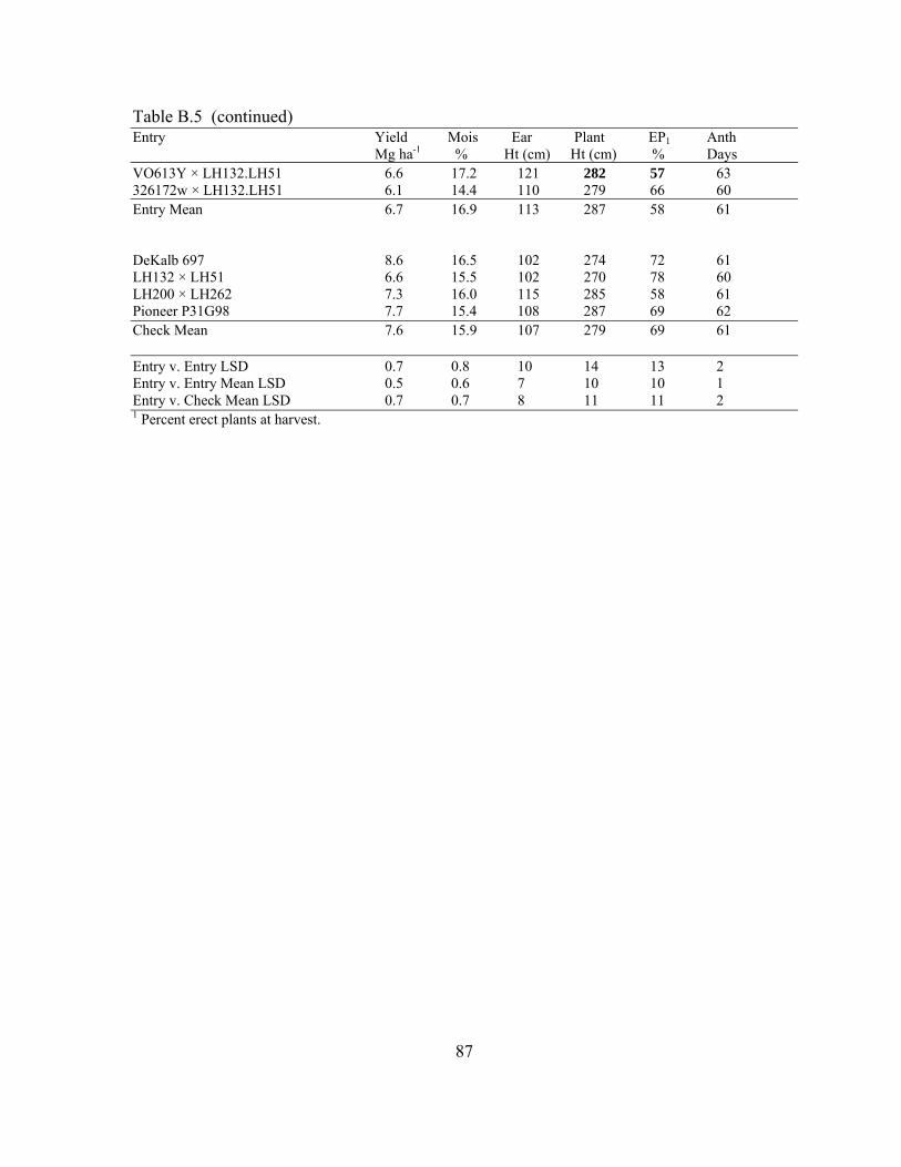
87
Table B.5 (continued) Entry Yield Mois Ear Plant EP1 Anth Mg ha-1 % Ht (cm) Ht (cm) % Days VO613Y × LH132.LH51 6.6 17.2 121 282 57 63 326172w × LH132.LH51 6.1 14.4 110 279 66 60 Entry Mean 6.7 16.9 113 287 58 61 DeKalb 697 8.6 16.5 102 274 72 61 LH132 × LH51 6.6 15.5 102 270 78 60 LH200 × LH262 7.3 16.0 115 285 58 61 Pioneer P31G98 7.7 15.4 108 287 69 62 Check Mean 7.6 15.9 107 279 69 61 Entry v. Entry LSD 0.7 0.8 10 14 13 2 Entry v. Entry Mean LSD 0.5 0.6 7 10 10 1 Entry v. Check Mean LSD 0.7 0.7 8 11 11 2 1 Percent erect plants at harvest.
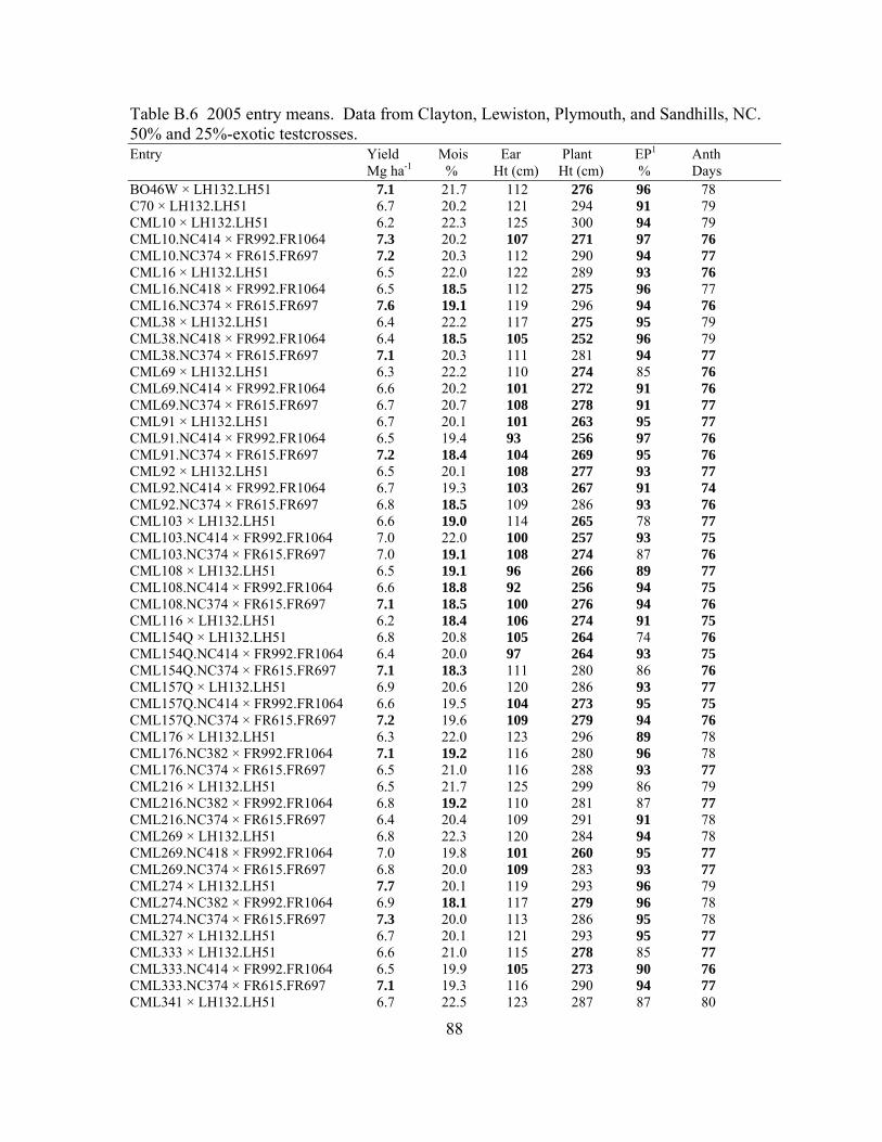
88
Table B.6 2005 entry means. Data from Clayton, Lewiston, Plymouth, and Sandhills, NC. 50% and 25%-exotic testcrosses. Entry Yield Mois Ear Plant EP1 Anth Mg ha-1 % Ht (cm) Ht (cm) % Days BO46W × LH132.LH51 7.1 21.7 112 276 96 78 C70 × LH132.LH51 6.7 20.2 121 294 91 79 CML10 × LH132.LH51 6.2 22.3 125 300 94 79 CML10.NC414 × FR992.FR1064 7.3 20.2 107 271 97 76 CML10.NC374 × FR615.FR697 7.2 20.3 112 290 94 77 CML16 × LH132.LH51 6.5 22.0 122 289 93 76 CML16.NC418 × FR992.FR1064 6.5 18.5 112 275 96 77 CML16.NC374 × FR615.FR697 7.6 19.1 119 296 94 76 CML38 × LH132.LH51 6.4 22.2 117 275 95 79 CML38.NC418 × FR992.FR1064 6.4 18.5 105 252 96 79 CML38.NC374 × FR615.FR697 7.1 20.3 111 281 94 77 CML69 × LH132.LH51 6.3 22.2 110 274 85 76 CML69.NC414 × FR992.FR1064 6.6 20.2 101 272 91 76 CML69.NC374 × FR615.FR697 6.7 20.7 108 278 91 77 CML91 × LH132.LH51 6.7 20.1 101 263 95 77 CML91.NC414 × FR992.FR1064 6.5 19.4 93 256 97 76 CML91.NC374 × FR615.FR697 7.2 18.4 104 269 95 76 CML92 × LH132.LH51 6.5 20.1 108 277 93 77 CML92.NC414 × FR992.FR1064 6.7 19.3 103 267 91 74 CML92.NC374 × FR615.FR697 6.8 18.5 109 286 93 76 CML103 × LH132.LH51 6.6 19.0 114 265 78 77 CML103.NC414 × FR992.FR1064 7.0 22.0 100 257 93 75 CML103.NC374 × FR615.FR697 7.0 19.1 108 274 87 76 CML108 × LH132.LH51 6.5 19.1 96 266 89 77 CML108.NC414 × FR992.FR1064 6.6 18.8 92 256 94 75 CML108.NC374 × FR615.FR697 7.1 18.5 100 276 94 76 CML116 × LH132.LH51 6.2 18.4 106 274 91 75 CML154Q × LH132.LH51 6.8 20.8 105 264 74 76 CML154Q.NC414 × FR992.FR1064 6.4 20.0 97 264 93 75 CML154Q.NC374 × FR615.FR697 7.1 18.3 111 280 86 76 CML157Q × LH132.LH51 6.9 20.6 120 286 93 77 CML157Q.NC414 × FR992.FR1064 6.6 19.5 104 273 95 75 CML157Q.NC374 × FR615.FR697 7.2 19.6 109 279 94 76 CML176 × LH132.LH51 6.3 22.0 123 296 89 78 CML176.NC382 × FR992.FR1064 7.1 19.2 116 280 96 78 CML176.NC374 × FR615.FR697 6.5 21.0 116 288 93 77 CML216 × LH132.LH51 6.5 21.7 125 299 86 79 CML216.NC382 × FR992.FR1064 6.8 19.2 110 281 87 77 CML216.NC374 × FR615.FR697 6.4 20.4 109 291 91 78 CML269 × LH132.LH51 6.8 22.3 120 284 94 78 CML269.NC418 × FR992.FR1064 7.0 19.8 101 260 95 77 CML269.NC374 × FR615.FR697 6.8 20.0 109 283 93 77 CML274 × LH132.LH51 7.7 20.1 119 293 96 79 CML274.NC382 × FR992.FR1064 6.9 18.1 117 279 96 78 CML274.NC374 × FR615.FR697 7.3 20.0 113 286 95 78 CML327 × LH132.LH51 6.7 20.1 121 293 95 77 CML333 × LH132.LH51 6.6 21.0 115 278 85 77 CML333.NC414 × FR992.FR1064 6.5 19.9 105 273 90 76 CML333.NC374 × FR615.FR697 7.1 19.3 116 290 94 77 CML341 × LH132.LH51 6.7 22.5 123 287 87 80
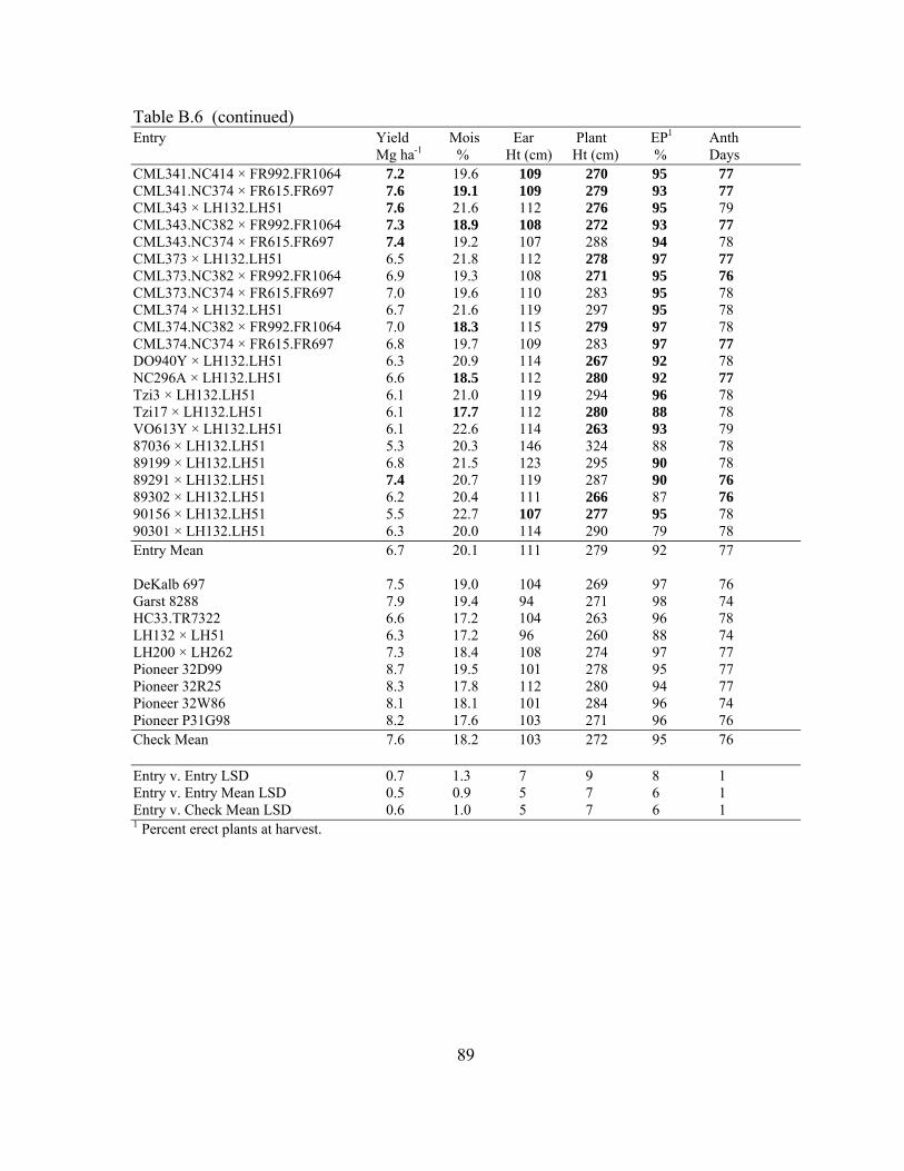
89
Table B.6 (continued) Entry Yield Mois Ear Plant EP1 Anth Mg ha-1 % Ht (cm) Ht (cm) % Days CML341.NC414 × FR992.FR1064 7.2 19.6 109 270 95 77 CML341.NC374 × FR615.FR697 7.6 19.1 109 279 93 77 CML343 × LH132.LH51 7.6 21.6 112 276 95 79 CML343.NC382 × FR992.FR1064 7.3 18.9 108 272 93 77 CML343.NC374 × FR615.FR697 7.4 19.2 107 288 94 78 CML373 × LH132.LH51 6.5 21.8 112 278 97 77 CML373.NC382 × FR992.FR1064 6.9 19.3 108 271 95 76 CML373.NC374 × FR615.FR697 7.0 19.6 110 283 95 78 CML374 × LH132.LH51 6.7 21.6 119 297 95 78 CML374.NC382 × FR992.FR1064 7.0 18.3 115 279 97 78 CML374.NC374 × FR615.FR697 6.8 19.7 109 283 97 77 DO940Y × LH132.LH51 6.3 20.9 114 267 92 78 NC296A × LH132.LH51 6.6 18.5 112 280 92 77 Tzi3 × LH132.LH51 6.1 21.0 119 294 96 78 Tzi17 × LH132.LH51 6.1 17.7 112 280 88 78 VO613Y × LH132.LH51 6.1 22.6 114 263 93 79 87036 × LH132.LH51 5.3 20.3 146 324 88 78 89199 × LH132.LH51 6.8 21.5 123 295 90 78 89291 × LH132.LH51 7.4 20.7 119 287 90 76 89302 × LH132.LH51 6.2 20.4 111 266 87 76 90156 × LH132.LH51 5.5 22.7 107 277 95 78 90301 × LH132.LH51 6.3 20.0 114 290 79 78 Entry Mean 6.7 20.1 111 279 92 77 DeKalb 697 7.5 19.0 104 269 97 76 Garst 8288 7.9 19.4 94 271 98 74 HC33.TR7322 6.6 17.2 104 263 96 78 LH132 × LH51 6.3 17.2 96 260 88 74 LH200 × LH262 7.3 18.4 108 274 97 77 Pioneer 32D99 8.7 19.5 101 278 95 77 Pioneer 32R25 8.3 17.8 112 280 94 77 Pioneer 32W86 8.1 18.1 101 284 96 74 Pioneer P31G98 8.2 17.6 103 271 96 76 Check Mean 7.6 18.2 103 272 95 76 Entry v. Entry LSD 0.7 1.3 7 9 8 1 Entry v. Entry Mean LSD 0.5 0.9 5 7 6 1 Entry v. Check Mean LSD 0.6 1.0 5 7 6 1 1 Percent erect plants at harvest.
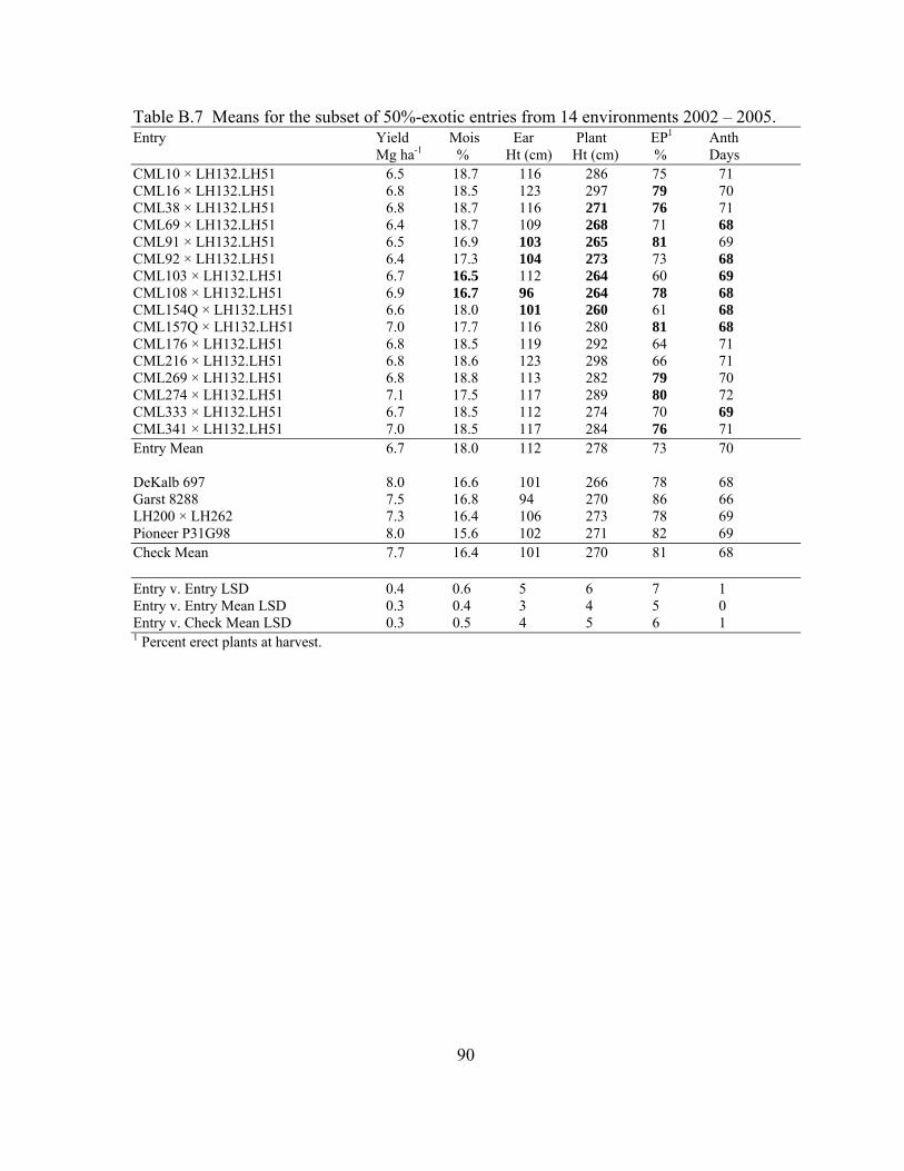
90
Table B.7 Means for the subset of 50%-exotic entries from 14 environments 2002 – 2005. Entry Yield Mois Ear Plant EPP
1 Anth Mg ha-1 % Ht (cm) Ht (cm) % Days CML10 × LH132.LH51 6.5 18.7 116 286 75 71 CML16 × LH132.LH51 6.8 18.5 123 297 79 70 CML38 × LH132.LH51 6.8 18.7 116 271 76 71 CML69 × LH132.LH51 6.4 18.7 109 268 71 68 CML91 × LH132.LH51 6.5 16.9 103 265 81 69 CML92 × LH132.LH51 6.4 17.3 104 273 73 68 CML103 × LH132.LH51 6.7 16.5 112 264 60 69 CML108 × LH132.LH51 6.9 16.7 96 264 78 68 CML154Q × LH132.LH51 6.6 18.0 101 260 61 68 CML157Q × LH132.LH51 7.0 17.7 116 280 81 68 CML176 × LH132.LH51 6.8 18.5 119 292 64 71 CML216 × LH132.LH51 6.8 18.6 123 298 66 71 CML269 × LH132.LH51 6.8 18.8 113 282 79 70 CML274 × LH132.LH51 7.1 17.5 117 289 80 72 CML333 × LH132.LH51 6.7 18.5 112 274 70 69 CML341 × LH132.LH51 7.0 18.5 117 284 76 71 Entry Mean 6.7 18.0 112 278 73 70 DeKalb 697 8.0 16.6 101 266 78 68 Garst 8288 7.5 16.8 94 270 86 66 LH200 × LH262 7.3 16.4 106 273 78 69 Pioneer P31G98 8.0 15.6 102 271 82 69 Check Mean 7.7 16.4 101 270 81 68 Entry v. Entry LSD 0.4 0.6 5 6 7 1 Entry v. Entry Mean LSD 0.3 0.4 3 4 5 0 Entry v. Check Mean LSD 0.3 0.5 4 5 6 1 1 Percent erect plants at harvest.
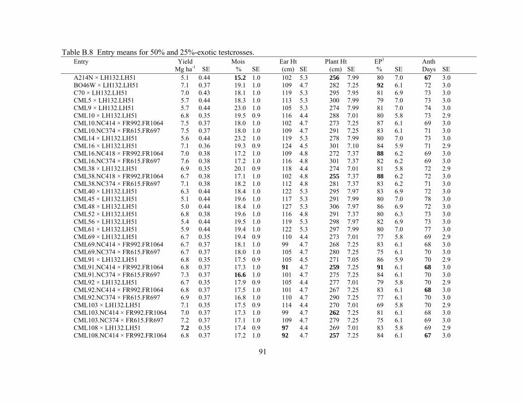
91
Table B.8 Entry means for 50% and 25%-exotic testcrosses. Entry Yield Mois Ear Ht Plant Ht EP1 Anth Mg ha-1 SE % SE (cm) SE (cm) SE % SE Days SE A214N × LH132.LH51 5.1 0.44 15.2 1.0 102 5.3 256 7.99 80 7.0 67 3.0 BO46W × LH132.LH51 7.1 0.37 19.1 1.0 109 4.7 282 7.25 92 6.1 72 3.0 C70 × LH132.LH51 7.0 0.43 18.1 1.0 119 5.3 295 7.95 81 6.9 73 3.0 CML5 × LH132.LH51 5.7 0.44 18.3 1.0 113 5.3 300 7.99 79 7.0 73 3.0 CML9 × LH132.LH51 5.7 0.44 23.0 1.0 105 5.3 274 7.99 81 7.0 74 3.0 CML10 × LH132.LH51 6.8 0.35 19.5 0.9 116 4.4 288 7.01 80 5.8 73 2.9 CML10.NC414 × FR992.FR1064 7.5 0.37 18.0 1.0 102 4.7 273 7.25 87 6.1 69 3.0 CML10.NC374 × FR615.FR697 7.5 0.37 18.0 1.0 109 4.7 291 7.25 83 6.1 71 3.0 CML14 × LH132.LH51 5.6 0.44 23.2 1.0 119 5.3 278 7.99 80 7.0 73 3.0 CML16 × LH132.LH51 7.1 0.36 19.3 0.9 124 4.5 301 7.10 84 5.9 71 2.9 CML16.NC418 × FR992.FR1064 7.0 0.38 17.2 1.0 109 4.8 272 7.37 88 6.2 69 3.0 CML16.NC374 × FR615.FR697 7.6 0.38 17.2 1.0 116 4.8 301 7.37 82 6.2 69 3.0 CML38 × LH132.LH51 6.9 0.35 20.1 0.9 118 4.4 274 7.01 81 5.8 72 2.9 CML38.NC418 × FR992.FR1064 6.7 0.38 17.1 1.0 102 4.8 255 7.37 88 6.2 72 3.0 CML38.NC374 × FR615.FR697 7.1 0.38 18.2 1.0 112 4.8 281 7.37 83 6.2 71 3.0 CML40 × LH132.LH51 6.3 0.44 18.4 1.0 122 5.3 295 7.97 83 6.9 72 3.0 CML45 × LH132.LH51 5.1 0.44 19.6 1.0 117 5.3 291 7.99 80 7.0 78 3.0 CML48 × LH132.LH51 5.0 0.44 18.4 1.0 127 5.3 306 7.97 86 6.9 72 3.0 CML52 × LH132.LH51 6.8 0.38 19.6 1.0 116 4.8 291 7.37 80 6.3 73 3.0 CML56 × LH132.LH51 5.4 0.44 19.5 1.0 119 5.3 298 7.97 82 6.9 73 3.0 CML61 × LH132.LH51 5.9 0.44 19.4 1.0 122 5.3 297 7.99 80 7.0 77 3.0 CML69 × LH132.LH51 6.7 0.35 19.4 0.9 110 4.4 273 7.01 77 5.8 69 2.9 CML69.NC414 × FR992.FR1064 6.7 0.37 18.1 1.0 99 4.7 268 7.25 83 6.1 68 3.0 CML69.NC374 × FR615.FR697 6.7 0.37 18.0 1.0 105 4.7 280 7.25 75 6.1 70 3.0 CML91 × LH132.LH51 6.8 0.35 17.5 0.9 105 4.5 271 7.05 86 5.9 70 2.9 CML91.NC414 × FR992.FR1064 6.8 0.37 17.3 1.0 91 4.7 259 7.25 91 6.1 68 3.0 CML91.NC374 × FR615.FR697 7.3 0.37 16.6 1.0 101 4.7 275 7.25 84 6.1 70 3.0 CML92 × LH132.LH51 6.7 0.35 17.9 0.9 105 4.4 277 7.01 79 5.8 70 2.9 CML92.NC414 × FR992.FR1064 6.8 0.37 17.5 1.0 101 4.7 267 7.25 83 6.1 68 3.0 CML92.NC374 × FR615.FR697 6.9 0.37 16.8 1.0 110 4.7 290 7.25 77 6.1 70 3.0 CML103 × LH132.LH51 7.1 0.35 17.5 0.9 114 4.4 270 7.01 69 5.8 70 2.9 CML103.NC414 × FR992.FR1064 7.0 0.37 17.3 1.0 99 4.7 262 7.25 81 6.1 68 3.0 CML103.NC374 × FR615.FR697 7.2 0.37 17.1 1.0 109 4.7 279 7.25 75 6.1 69 3.0 CML108 × LH132.LH51 7.2 0.35 17.4 0.9 97 4.4 269 7.01 83 5.8 69 2.9 CML108.NC414 × FR992.FR1064 6.8 0.37 17.2 1.0 92 4.7 257 7.25 84 6.1 67 3.0
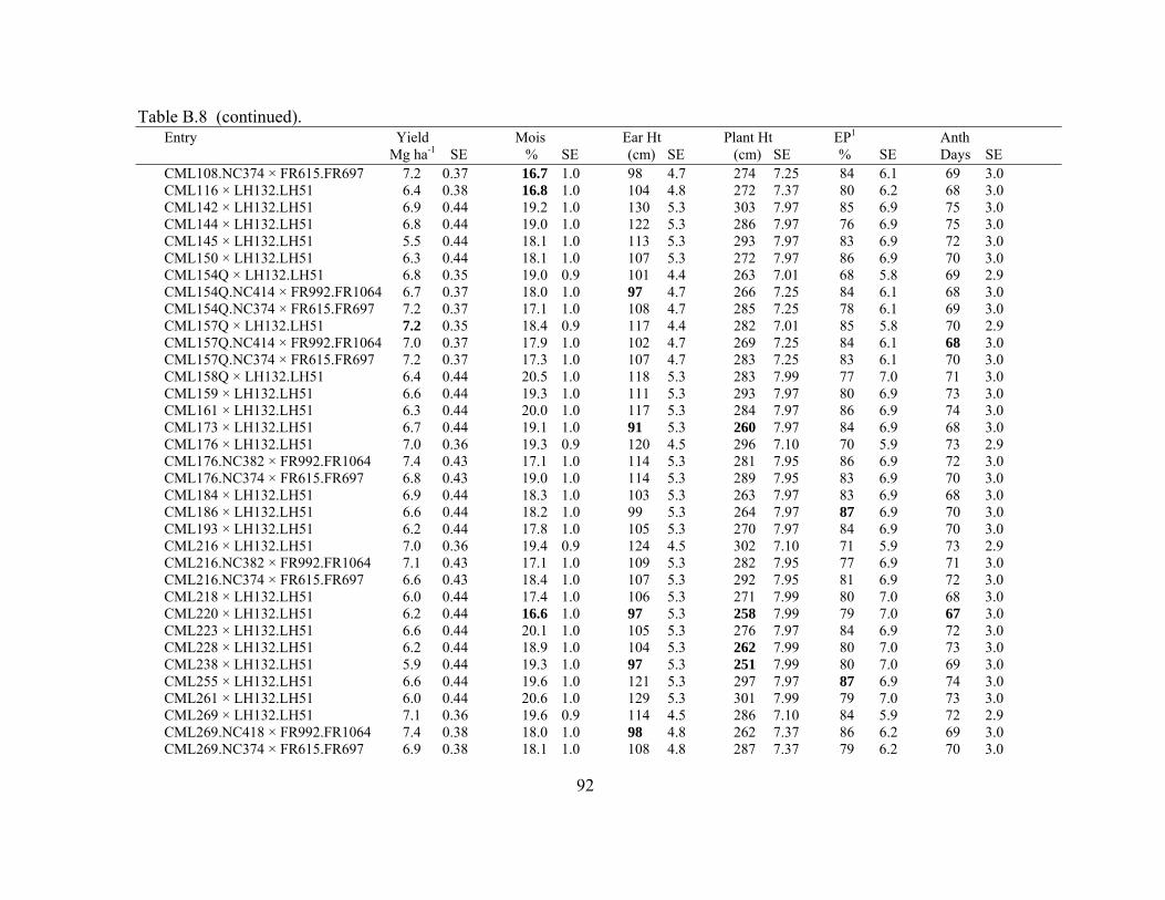
92
Table B.8 (continued). Entry Yield Mois Ear Ht Plant Ht EP1 Anth Mg ha-1 SE % SE (cm) SE (cm) SE % SE Days SE CML108.NC374 × FR615.FR697 7.2 0.37 16.7 1.0 98 4.7 274 7.25 84 6.1 69 3.0 CML116 × LH132.LH51 6.4 0.38 16.8 1.0 104 4.8 272 7.37 80 6.2 68 3.0 CML142 × LH132.LH51 6.9 0.44 19.2 1.0 130 5.3 303 7.97 85 6.9 75 3.0 CML144 × LH132.LH51 6.8 0.44 19.0 1.0 122 5.3 286 7.97 76 6.9 75 3.0 CML145 × LH132.LH51 5.5 0.44 18.1 1.0 113 5.3 293 7.97 83 6.9 72 3.0 CML150 × LH132.LH51 6.3 0.44 18.1 1.0 107 5.3 272 7.97 86 6.9 70 3.0 CML154Q × LH132.LH51 6.8 0.35 19.0 0.9 101 4.4 263 7.01 68 5.8 69 2.9 CML154Q.NC414 × FR992.FR1064 6.7 0.37 18.0 1.0 97 4.7 266 7.25 84 6.1 68 3.0 CML154Q.NC374 × FR615.FR697 7.2 0.37 17.1 1.0 108 4.7 285 7.25 78 6.1 69 3.0 CML157Q × LH132.LH51 7.2 0.35 18.4 0.9 117 4.4 282 7.01 85 5.8 70 2.9 CML157Q.NC414 × FR992.FR1064 7.0 0.37 17.9 1.0 102 4.7 269 7.25 84 6.1 68 3.0 CML157Q.NC374 × FR615.FR697 7.2 0.37 17.3 1.0 107 4.7 283 7.25 83 6.1 70 3.0 CML158Q × LH132.LH51 6.4 0.44 20.5 1.0 118 5.3 283 7.99 77 7.0 71 3.0 CML159 × LH132.LH51 6.6 0.44 19.3 1.0 111 5.3 293 7.97 80 6.9 73 3.0 CML161 × LH132.LH51 6.3 0.44 20.0 1.0 117 5.3 284 7.97 86 6.9 74 3.0 CML173 × LH132.LH51 6.7 0.44 19.1 1.0 91 5.3 260 7.97 84 6.9 68 3.0 CML176 × LH132.LH51 7.0 0.36 19.3 0.9 120 4.5 296 7.10 70 5.9 73 2.9 CML176.NC382 × FR992.FR1064 7.4 0.43 17.1 1.0 114 5.3 281 7.95 86 6.9 72 3.0 CML176.NC374 × FR615.FR697 6.8 0.43 19.0 1.0 114 5.3 289 7.95 83 6.9 70 3.0 CML184 × LH132.LH51 6.9 0.44 18.3 1.0 103 5.3 263 7.97 83 6.9 68 3.0 CML186 × LH132.LH51 6.6 0.44 18.2 1.0 99 5.3 264 7.97 87 6.9 70 3.0 CML193 × LH132.LH51 6.2 0.44 17.8 1.0 105 5.3 270 7.97 84 6.9 70 3.0 CML216 × LH132.LH51 7.0 0.36 19.4 0.9 124 4.5 302 7.10 71 5.9 73 2.9 CML216.NC382 × FR992.FR1064 7.1 0.43 17.1 1.0 109 5.3 282 7.95 77 6.9 71 3.0 CML216.NC374 × FR615.FR697 6.6 0.43 18.4 1.0 107 5.3 292 7.95 81 6.9 72 3.0 CML218 × LH132.LH51 6.0 0.44 17.4 1.0 106 5.3 271 7.99 80 7.0 68 3.0 CML220 × LH132.LH51 6.2 0.44 16.6 1.0 97 5.3 258 7.99 79 7.0 67 3.0 CML223 × LH132.LH51 6.6 0.44 20.1 1.0 105 5.3 276 7.97 84 6.9 72 3.0 CML228 × LH132.LH51 6.2 0.44 18.9 1.0 104 5.3 262 7.99 80 7.0 73 3.0 CML238 × LH132.LH51 5.9 0.44 19.3 1.0 97 5.3 251 7.99 80 7.0 69 3.0 CML255 × LH132.LH51 6.6 0.44 19.6 1.0 121 5.3 297 7.97 87 6.9 74 3.0 CML261 × LH132.LH51 6.0 0.44 20.6 1.0 129 5.3 301 7.99 79 7.0 73 3.0 CML269 × LH132.LH51 7.1 0.36 19.6 0.9 114 4.5 286 7.10 84 5.9 72 2.9 CML269.NC418 × FR992.FR1064 7.4 0.38 18.0 1.0 98 4.8 262 7.37 86 6.2 69 3.0 CML269.NC374 × FR615.FR697 6.9 0.38 18.1 1.0 108 4.8 287 7.37 79 6.2 70 3.0
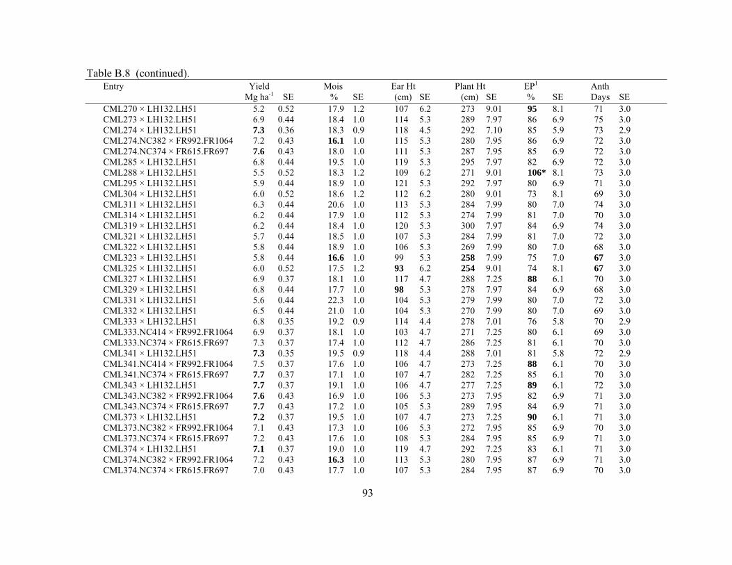
93
Table B.8 (continued). Entry Yield Mois Ear Ht Plant Ht EP1 Anth Mg ha-1 SE % SE (cm) SE (cm) SE % SE Days SE CML270 × LH132.LH51 5.2 0.52 17.9 1.2 107 6.2 273 9.01 95 8.1 71 3.0 CML273 × LH132.LH51 6.9 0.44 18.4 1.0 114 5.3 289 7.97 86 6.9 75 3.0 CML274 × LH132.LH51 7.3 0.36 18.3 0.9 118 4.5 292 7.10 85 5.9 73 2.9 CML274.NC382 × FR992.FR1064 7.2 0.43 16.1 1.0 115 5.3 280 7.95 86 6.9 72 3.0 CML274.NC374 × FR615.FR697 7.6 0.43 18.0 1.0 111 5.3 287 7.95 85 6.9 72 3.0 CML285 × LH132.LH51 6.8 0.44 19.5 1.0 119 5.3 295 7.97 82 6.9 72 3.0 CML288 × LH132.LH51 5.5 0.52 18.3 1.2 109 6.2 271 9.01 106* 8.1 73 3.0 CML295 × LH132.LH51 5.9 0.44 18.9 1.0 121 5.3 292 7.97 80 6.9 71 3.0 CML304 × LH132.LH51 6.0 0.52 18.6 1.2 112 6.2 280 9.01 73 8.1 69 3.0 CML311 × LH132.LH51 6.3 0.44 20.6 1.0 113 5.3 284 7.99 80 7.0 74 3.0 CML314 × LH132.LH51 6.2 0.44 17.9 1.0 112 5.3 274 7.99 81 7.0 70 3.0 CML319 × LH132.LH51 6.2 0.44 18.4 1.0 120 5.3 300 7.97 84 6.9 74 3.0 CML321 × LH132.LH51 5.7 0.44 18.5 1.0 107 5.3 284 7.99 81 7.0 72 3.0 CML322 × LH132.LH51 5.8 0.44 18.9 1.0 106 5.3 269 7.99 80 7.0 68 3.0 CML323 × LH132.LH51 5.8 0.44 16.6 1.0 99 5.3 258 7.99 75 7.0 67 3.0 CML325 × LH132.LH51 6.0 0.52 17.5 1.2 93 6.2 254 9.01 74 8.1 67 3.0 CML327 × LH132.LH51 6.9 0.37 18.1 1.0 117 4.7 288 7.25 88 6.1 70 3.0 CML329 × LH132.LH51 6.8 0.44 17.7 1.0 98 5.3 278 7.97 84 6.9 68 3.0 CML331 × LH132.LH51 5.6 0.44 22.3 1.0 104 5.3 279 7.99 80 7.0 72 3.0 CML332 × LH132.LH51 6.5 0.44 21.0 1.0 104 5.3 270 7.99 80 7.0 69 3.0 CML333 × LH132.LH51 6.8 0.35 19.2 0.9 114 4.4 278 7.01 76 5.8 70 2.9 CML333.NC414 × FR992.FR1064 6.9 0.37 18.1 1.0 103 4.7 271 7.25 80 6.1 69 3.0 CML333.NC374 × FR615.FR697 7.3 0.37 17.4 1.0 112 4.7 286 7.25 81 6.1 70 3.0 CML341 × LH132.LH51 7.3 0.35 19.5 0.9 118 4.4 288 7.01 81 5.8 72 2.9 CML341.NC414 × FR992.FR1064 7.5 0.37 17.6 1.0 106 4.7 273 7.25 88 6.1 70 3.0 CML341.NC374 × FR615.FR697 7.7 0.37 17.1 1.0 107 4.7 282 7.25 85 6.1 70 3.0 CML343 × LH132.LH51 7.7 0.37 19.1 1.0 106 4.7 277 7.25 89 6.1 72 3.0 CML343.NC382 × FR992.FR1064 7.6 0.43 16.9 1.0 106 5.3 273 7.95 82 6.9 71 3.0 CML343.NC374 × FR615.FR697 7.7 0.43 17.2 1.0 105 5.3 289 7.95 84 6.9 71 3.0 CML373 × LH132.LH51 7.2 0.37 19.5 1.0 107 4.7 273 7.25 90 6.1 71 3.0 CML373.NC382 × FR992.FR1064 7.1 0.43 17.3 1.0 106 5.3 272 7.95 85 6.9 70 3.0 CML373.NC374 × FR615.FR697 7.2 0.43 17.6 1.0 108 5.3 284 7.95 85 6.9 71 3.0 CML374 × LH132.LH51 7.1 0.37 19.0 1.0 119 4.7 292 7.25 83 6.1 71 3.0 CML374.NC382 × FR992.FR1064 7.2 0.43 16.3 1.0 113 5.3 280 7.95 87 6.9 71 3.0 CML374.NC374 × FR615.FR697 7.0 0.43 17.7 1.0 107 5.3 284 7.95 87 6.9 70 3.0
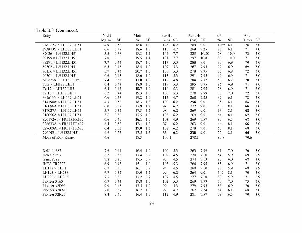
94
Table B.8 (continued). Entry Yield Mois Ear Ht Plant Ht EP1 Anth Mg ha-1 SE % SE (cm) SE (cm) SE % SE Days SE CML384 × LH132.LH51 4.9 0.52 18.6 1.2 123 6.2 289 9.01 106* 8.1 76 3.0 DO940Y × LH132.LH51 6.6 0.37 18.6 1.0 110 4.7 269 7.25 85 6.1 71 3.0 87036 × LH132.LH51 5.5 0.66 18.3 1.4 144 7.7 325 10.80 78 10.0 72 3.0 89199 × LH132.LH51 7.0 0.66 19.5 1.4 121 7.7 297 10.8 80 10.0 71 3.0 89291 × LH132.LH51 7.7 0.43 18.7 1.0 117 5.3 288 8.0 80 6.9 70 3.0 89302 × LH132.LH51 6.5 0.43 18.4 1.0 109 5.3 267 7.95 77 6.9 69 3.0 90156 × LH132.LH51 5.7 0.43 20.7 1.0 106 5.3 278 7.95 85 6.9 72 3.0 90301 × LH132.LH51 6.6 0.43 18.0 1.0 113 5.3 291 7.95 69 6.9 71 3.0 NC296A × LH132.LH51 7.4 0.38 17.0 1.0 112 4.8 284 7.37 83 6.2 70 3.0 Tzi3 × LH132.LH51 6.4 0.43 18.9 1.0 117 5.3 295 7.95 86 6.9 71 3.0 Tzi17 × LH132.LH51 6.4 0.43 15.7 1.0 110 5.3 281 7.95 78 6.9 71 3.0 Tzi18 × LH132.LH51 6.2 0.44 19.3 1.0 106 5.3 270 7.99 77 7.0 72 3.0 VO613Y × LH132.LH51 6.6 0.37 19.2 1.0 113 4.7 268 7.25 82 6.1 72 3.0 314190w × LH132.LH51 4.3 0.52 18.3 1.2 100 6.2 256 9.01 38 8.1 68 3.0 316096A × LH132.LH51 6.0 0.52 17.9 1.2 92 6.2 272 9.01 63 8.1 66 3.0 317027A × LH132.LH51 5.7 0.52 17.3 1.2 98 6.2 269 9.01 63 8.1 68 3.0 318056A × LH132.LH51 5.6 0.52 17.5 1.2 103 6.2 269 9.01 64 8.1 67 3.0 326172w. × FR615.FR697 6.6 0.40 16.1 1.0 103 4.9 269 7.57 80 6.5 68 3.0 326633A. × FR615.FR697 6.4 0.52 17.1 1.2 87 6.2 263 9.01 66 8.1 66 3.0 327609A. × FR615.FR697 6.4 0.52 17.0 1.2 102 6.2 278 9.01 67 8.1 68 3.0 796 NS × LH132.LH51 4.9 0.52 17.5 1.2 85 6.2 238 9.01 72 8.1 66 3.0 Mean of Exp. Entries 6.6 18.3 109.1 278.8 80.8 70.6 DeKalb 687 7.6 0.44 16.4 1.0 100 5.3 263 7.99 81 7.0 70 3.0 DeKalb 697 8.2 0.36 17.4 0.9 102 4.5 270 7.10 84 5.9 69 2.9 Garst 8288 7.8 0.36 17.5 0.9 95 4.5 274 7.13 92 6.0 68 3.0 HC33.TR7322 6.9 0.43 15.1 1.0 103 5.3 264 7.95 85 6.9 71 3.0 LH132 × LH51 6.7 0.36 16.1 0.9 94 4.5 260 7.10 82 5.9 68 2.9 LH195 × LH256 6.7 0.52 18.0 1.2 99 6.2 264 9.01 102 8.1 70 3.0 LH200 × LH262 7.5 0.36 17.2 0.9 107 4.5 277 7.10 83 5.9 71 2.9 Pioneer 3165 6.9 0.44 19.8 1.0 102 5.3 269 7.99 78 7.0 73 3.0 Pioneer 32D99 9.0 0.43 17.5 1.0 99 5.3 279 7.95 85 6.9 70 3.0 Pioneer 32K61 7.0 0.37 16.7 1.0 92 4.7 267 7.24 84 6.1 68 3.0 Pioneer 32R25 8.4 0.40 16.4 1.0 112 4.9 281 7.57 73 6.5 70 3.0
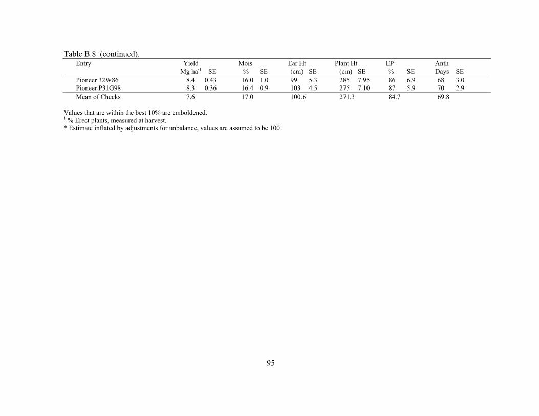
95
Table B.8 (continued). Entry Yield Mois Ear Ht Plant Ht EP1 Anth Mg ha-1 SE % SE (cm) SE (cm) SE % SE Days SE Pioneer 32W86 8.4 0.43 16.0 1.0 99 5.3 285 7.95 86 6.9 68 3.0 Pioneer P31G98 8.3 0.36 16.4 0.9 103 4.5 275 7.10 87 5.9 70 2.9 Mean of Checks 7.6 17.0 100.6 271.3 84.7 69.8 Values that are within the best 10% are emboldened. 1 % Erect plants, measured at harvest. * Estimate inflated by adjustments for unbalance, values are assumed to be 100.
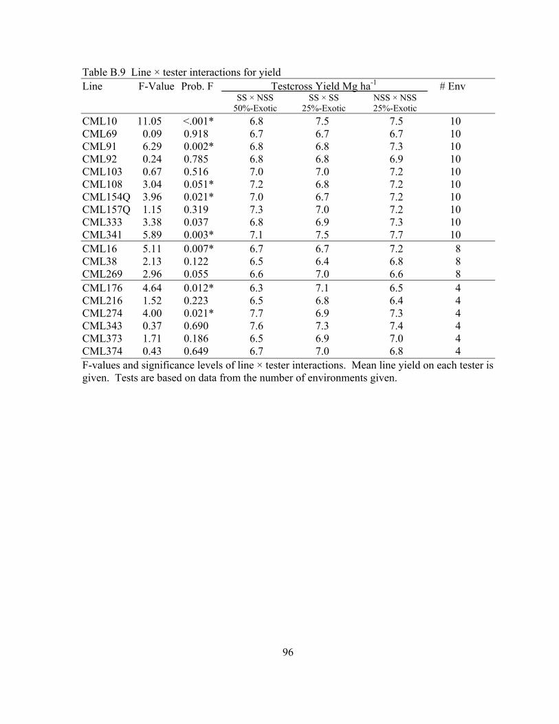
Table B.9 Line × tester interactions for yield Line F-Value Prob. F Testcross Yield Mg ha-1 # Env SS × NSS SS × SS NSS × NSS 50%-Exotic 25%-Exotic 25%-Exotic CML10 11.05 <.001* 6.8 7.5 7.5 10 CML69 0.09 0.918 6.7 6.7 6.7 10 CML91 6.29 0.002* 6.8 6.8 7.3 10 CML92 0.24 0.785 6.8 6.8 6.9 10 CML103 0.67 0.516 7.0 7.0 7.2 10 CML108 3.04 0.051* 7.2 6.8 7.2 10 CML154Q 3.96 0.021* 7.0 6.7 7.2 10 CML157Q 1.15 0.319 7.3 7.0 7.2 10 CML333 3.38 0.037 6.8 6.9 7.3 10 CML341 5.89 0.003* 7.1 7.5 7.7 10 CML16 5.11 0.007* 6.7 6.7 7.2 8 CML38 2.13 0.122 6.5 6.4 6.8 8 CML269 2.96 0.055 6.6 7.0 6.6 8 CML176 4.64 0.012* 6.3 7.1 6.5 4 CML216 1.52 0.223 6.5 6.8 6.4 4 CML274 4.00 0.021* 7.7 6.9 7.3 4 CML343 0.37 0.690 7.6 7.3 7.4 4 CML373 1.71 0.186 6.5 6.9 7.0 4 CML374 0.43 0.649 6.7 7.0 6.8 4 F-values and significance levels of line × tester interactions. Mean line yield on each tester is given. Tests are based on data from the number of environments given.
96
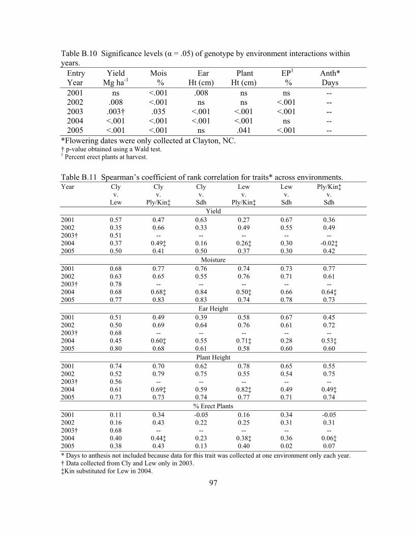
97
Table B.10 Significance levels (α = .05) of genotype by environment interactions within years. Entry Yield Mois Ear Plant EP1 Anth* Year Mg ha-1 % Ht (cm) Ht (cm) % Days 2001 ns <.001 .008 ns ns -- 2002 .008 <.001 ns ns <.001 -- 2003 .003† .035 <.001 <.001 <.001 -- 2004 <.001 <.001 <.001 <.001 ns -- 2005 <.001 <.001 ns .041 <.001 -- *Flowering dates were only collected at Clayton, NC. † p-value obtained using a Wald test. 1 Percent erect plants at harvest.
Table B.11 Spearman’s coefficient of rank correlation for traits* across environments. Year Cly Cly Cly Lew Lew Ply/Kin‡ v. v. v. v. v. v. Lew Ply/Kin‡ Sdh Ply/Kin‡ Sdh Sdh
Yield 2001 0.57 0.47 0.63 0.27 0.67 0.36 2002 0.35 0.66 0.33 0.49 0.55 0.49 2003† 0.51 -- -- -- -- -- 2004 0.37 0.49‡ 0.16 0.26‡ 0.30 -0.02‡ 2005 0.50 0.41 0.50 0.37 0.30 0.42
Moisture 2001 0.68 0.77 0.76 0.74 0.73 0.77 2002 0.63 0.65 0.55 0.76 0.71 0.61 2003† 0.78 -- -- -- -- -- 2004 0.68 0.68‡ 0.84 0.50‡ 0.66 0.64‡ 2005 0.77 0.83 0.83 0.74 0.78 0.73
Ear Height 2001 0.51 0.49 0.39 0.58 0.67 0.45 2002 0.50 0.69 0.64 0.76 0.61 0.72 2003† 0.68 -- -- -- -- -- 2004 0.45 0.60‡ 0.55 0.71‡ 0.28 0.53‡ 2005 0.80 0.68 0.61 0.58 0.60 0.60
Plant Height 2001 0.74 0.70 0.62 0.78 0.65 0.55 2002 0.52 0.79 0.75 0.55 0.54 0.75 2003† 0.56 -- -- -- -- -- 2004 0.61 0.69‡ 0.59 0.82‡ 0.49 0.49‡ 2005 0.73 0.73 0.74 0.77 0.71 0.74
% Erect Plants 2001 0.11 0.34 -0.05 0.16 0.34 -0.05 2002 0.16 0.43 0.22 0.25 0.31 0.31 2003† 0.68 -- -- -- -- -- 2004 0.40 0.44‡ 0.23 0.38‡ 0.36 0.06‡ 2005 0.38 0.43 0.13 0.40 0.02 0.07 * Days to anthesis not included because data for this trait was collected at one environment only each year. † Data collected from Cly and Lew only in 2003. ‡Kin substituted for Lew in 2004.
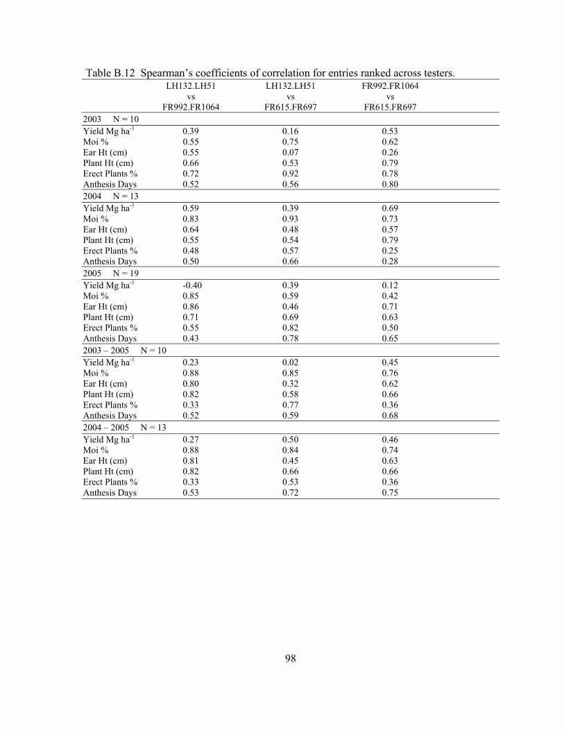
98
Table B.12 Spearman’s coefficients of correlation for entries ranked across testers. LH132.LH51 LH132.LH51 FR992.FR1064 vs vs vs FR992.FR1064 FR615.FR697 FR615.FR697 2003 N = 10 Yield Mg ha-1 0.39 0.16 0.53 Moi % 0.55 0.75 0.62 Ear Ht (cm) 0.55 0.07 0.26 Plant Ht (cm) 0.66 0.53 0.79 Erect Plants % 0.72 0.92 0.78 Anthesis Days 0.52 0.56 0.80 2004 N = 13 Yield Mg ha-1 0.59 0.39 0.69 Moi % 0.83 0.93 0.73 Ear Ht (cm) 0.64 0.48 0.57 Plant Ht (cm) 0.55 0.54 0.79 Erect Plants % 0.48 0.57 0.25 Anthesis Days 0.50 0.66 0.28 2005 N = 19 Yield Mg ha-1 -0.40 0.39 0.12 Moi % 0.85 0.59 0.42 Ear Ht (cm) 0.86 0.46 0.71 Plant Ht (cm) 0.71 0.69 0.63 Erect Plants % 0.55 0.82 0.50 Anthesis Days 0.43 0.78 0.65 2003 – 2005 N = 10 Yield Mg ha-1 0.23 0.02 0.45 Moi % 0.88 0.85 0.76 Ear Ht (cm) 0.80 0.32 0.62 Plant Ht (cm) 0.82 0.58 0.66 Erect Plants % 0.33 0.77 0.36 Anthesis Days 0.52 0.59 0.68 2004 – 2005 N = 13 Yield Mg ha-1 0.27 0.50 0.46 Moi % 0.88 0.84 0.74 Ear Ht (cm) 0.81 0.45 0.63 Plant Ht (cm) 0.82 0.66 0.66 Erect Plants % 0.33 0.53 0.36 Anthesis Days 0.53 0.72 0.75
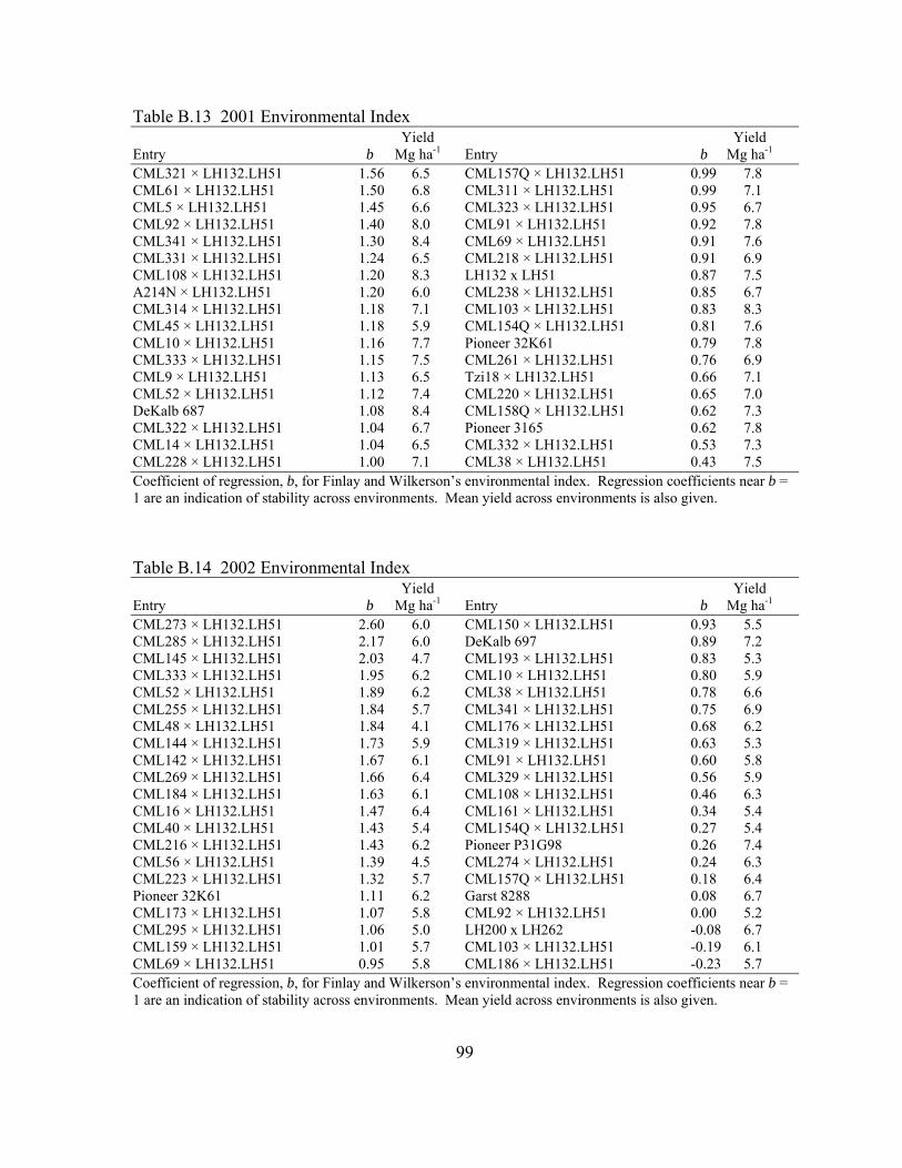
99
Table B.13 2001 Environmental Index Yield Yield Entry b Mg ha-1 Entry b Mg ha-1 CML321 × LH132.LH51 1.56 6.5 CML157Q × LH132.LH51 0.99 7.8 CML61 × LH132.LH51 1.50 6.8 CML311 × LH132.LH51 0.99 7.1 CML5 × LH132.LH51 1.45 6.6 CML323 × LH132.LH51 0.95 6.7 CML92 × LH132.LH51 1.40 8.0 CML91 × LH132.LH51 0.92 7.8 CML341 × LH132.LH51 1.30 8.4 CML69 × LH132.LH51 0.91 7.6 CML331 × LH132.LH51 1.24 6.5 CML218 × LH132.LH51 0.91 6.9 CML108 × LH132.LH51 1.20 8.3 LH132 x LH51 0.87 7.5 A214N × LH132.LH51 1.20 6.0 CML238 × LH132.LH51 0.85 6.7 CML314 × LH132.LH51 1.18 7.1 CML103 × LH132.LH51 0.83 8.3 CML45 × LH132.LH51 1.18 5.9 CML154Q × LH132.LH51 0.81 7.6 CML10 × LH132.LH51 1.16 7.7 Pioneer 32K61 0.79 7.8 CML333 × LH132.LH51 1.15 7.5 CML261 × LH132.LH51 0.76 6.9 CML9 × LH132.LH51 1.13 6.5 Tzi18 × LH132.LH51 0.66 7.1 CML52 × LH132.LH51 1.12 7.4 CML220 × LH132.LH51 0.65 7.0 DeKalb 687 1.08 8.4 CML158Q × LH132.LH51 0.62 7.3 CML322 × LH132.LH51 1.04 6.7 Pioneer 3165 0.62 7.8 CML14 × LH132.LH51 1.04 6.5 CML332 × LH132.LH51 0.53 7.3 CML228 × LH132.LH51 1.00 7.1 CML38 × LH132.LH51 0.43 7.5 Coefficient of regression, b, for Finlay and Wilkerson’s environmental index. Regression coefficients near b = 1 are an indication of stability across environments. Mean yield across environments is also given. Table B.14 2002 Environmental Index Yield Yield Entry b Mg ha-1 Entry b Mg ha-1 CML273 × LH132.LH51 2.60 6.0 CML150 × LH132.LH51 0.93 5.5 CML285 × LH132.LH51 2.17 6.0 DeKalb 697 0.89 7.2 CML145 × LH132.LH51 2.03 4.7 CML193 × LH132.LH51 0.83 5.3 CML333 × LH132.LH51 1.95 6.2 CML10 × LH132.LH51 0.80 5.9 CML52 × LH132.LH51 1.89 6.2 CML38 × LH132.LH51 0.78 6.6 CML255 × LH132.LH51 1.84 5.7 CML341 × LH132.LH51 0.75 6.9 CML48 × LH132.LH51 1.84 4.1 CML176 × LH132.LH51 0.68 6.2 CML144 × LH132.LH51 1.73 5.9 CML319 × LH132.LH51 0.63 5.3 CML142 × LH132.LH51 1.67 6.1 CML91 × LH132.LH51 0.60 5.8 CML269 × LH132.LH51 1.66 6.4 CML329 × LH132.LH51 0.56 5.9 CML184 × LH132.LH51 1.63 6.1 CML108 × LH132.LH51 0.46 6.3 CML16 × LH132.LH51 1.47 6.4 CML161 × LH132.LH51 0.34 5.4 CML40 × LH132.LH51 1.43 5.4 CML154Q × LH132.LH51 0.27 5.4 CML216 × LH132.LH51 1.43 6.2 Pioneer P31G98 0.26 7.4 CML56 × LH132.LH51 1.39 4.5 CML274 × LH132.LH51 0.24 6.3 CML223 × LH132.LH51 1.32 5.7 CML157Q × LH132.LH51 0.18 6.4 Pioneer 32K61 1.11 6.2 Garst 8288 0.08 6.7 CML173 × LH132.LH51 1.07 5.8 CML92 × LH132.LH51 0.00 5.2 CML295 × LH132.LH51 1.06 5.0 LH200 x LH262 -0.08 6.7 CML159 × LH132.LH51 1.01 5.7 CML103 × LH132.LH51 -0.19 6.1 CML69 × LH132.LH51 0.95 5.8 CML186 × LH132.LH51 -0.23 5.7 Coefficient of regression, b, for Finlay and Wilkerson’s environmental index. Regression coefficients near b = 1 are an indication of stability across environments. Mean yield across environments is also given.
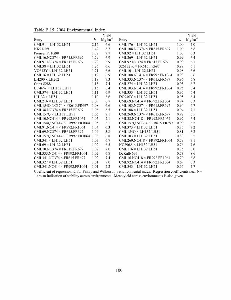
100
Table B.15 2004 Environmental Index Yield Yield Entry b Mg ha-1 Entry b Mg ha-1 CML91 × LH132.LH51 2.15 6.6 CML176 × LH132.LH51 1.00 7.0 NK91-R9 1.42 6.7 CML108.NC374 × FR615.FR697 1.00 6.8 Pioneer P31G98 1.38 7.7 CML92 × LH132.LH51 1.00 6.3 CML16.NC374 × FR615.FR697 1.29 6.9 CML269 × LH132.LH51 0.99 6.4 CML91.NC374 × FR615.FR697 1.29 6.9 CML92.NC374 × FR615.FR697 0.99 6.1 CML38 × LH132.LH51 1.26 6.6 326172w. × FR615.FR697 0.99 6.1 VO613Y × LH132.LH51 1.21 6.6 CML10 × LH132.LH51 0.98 6.6 CML16 × LH132.LH51 1.19 6.9 CML108.NC414 × FR992.FR1064 0.98 6.6 LH200 x LH262 1.18 7.3 CML333.NC374 × FR615.FR697 0.96 6.8 Garst 8288 1.15 7.4 CML274 × LH132.LH51 0.95 6.7 BO46W × LH132.LH51 1.15 6.4 CML103.NC414 × FR992.FR1064 0.95 6.4 CML374 × LH132.LH51 1.11 6.9 CML333 × LH132.LH51 0.95 6.4 LH132 x LH51 1.10 6.6 DO940Y × LH132.LH51 0.95 6.4 CML216 × LH132.LH51 1.09 6.7 CML69.NC414 × FR992.FR1064 0.94 6.3 CML154Q.NC374 × FR615.FR697 1.08 6.6 CML103.NC374 × FR615.FR697 0.94 6.7 CML38.NC374 × FR615.FR697 1.06 6.5 CML108 × LH132.LH51 0.94 7.1 CML157Q × LH132.LH51 1.06 7.1 CML269.NC374 × FR615.FR697 0.92 6.5 CML10.NC414 × FR992.FR1064 1.05 7.1 CML38.NC418 × FR992.FR1064 0.92 6.4 CML154Q.NC414 × FR992.FR1064 1.05 6.1 CML157Q.NC374 × FR615.FR697 0.90 6.5 CML91.NC414 × FR992.FR1064 1.04 6.3 CML373 × LH132.LH51 0.85 7.2 CML69.NC374 × FR615.FR697 1.04 5.8 CML154Q × LH132.LH51 0.81 6.2 CML157Q.NC414 × FR992.FR1064 1.03 6.8 CML103 × LH132.LH51 0.80 6.5 CML341 × LH132.LH51 1.03 6.7 CML269.NC418 × FR992.FR1064 0.79 7.1 CML69 × LH132.LH51 1.02 6.5 NC296A × LH132.LH51 0.76 7.6 CML10.NC374 × FR615.FR697 1.02 7.0 CML116 × LH132.LH51 0.75 6.0 CML333.NC414 × FR992.FR1064 1.02 6.8 DeKalb 697 0.73 8.6 CML341.NC374 × FR615.FR697 1.02 7.4 CML16.NC418 × FR992.FR1064 0.70 6.8 CML327 × LH132.LH51 1.01 7.0 CML92.NC414 × FR992.FR1064 0.69 6.3 CML341.NC414 × FR992.FR1064 1.01 7.2 CML343 × LH132.LH51 0.66 7.7 Coefficient of regression, b, for Finlay and Wilkerson’s environmental index. Regression coefficients near b = 1 are an indication of stability across environments. Mean yield across environments is also given.
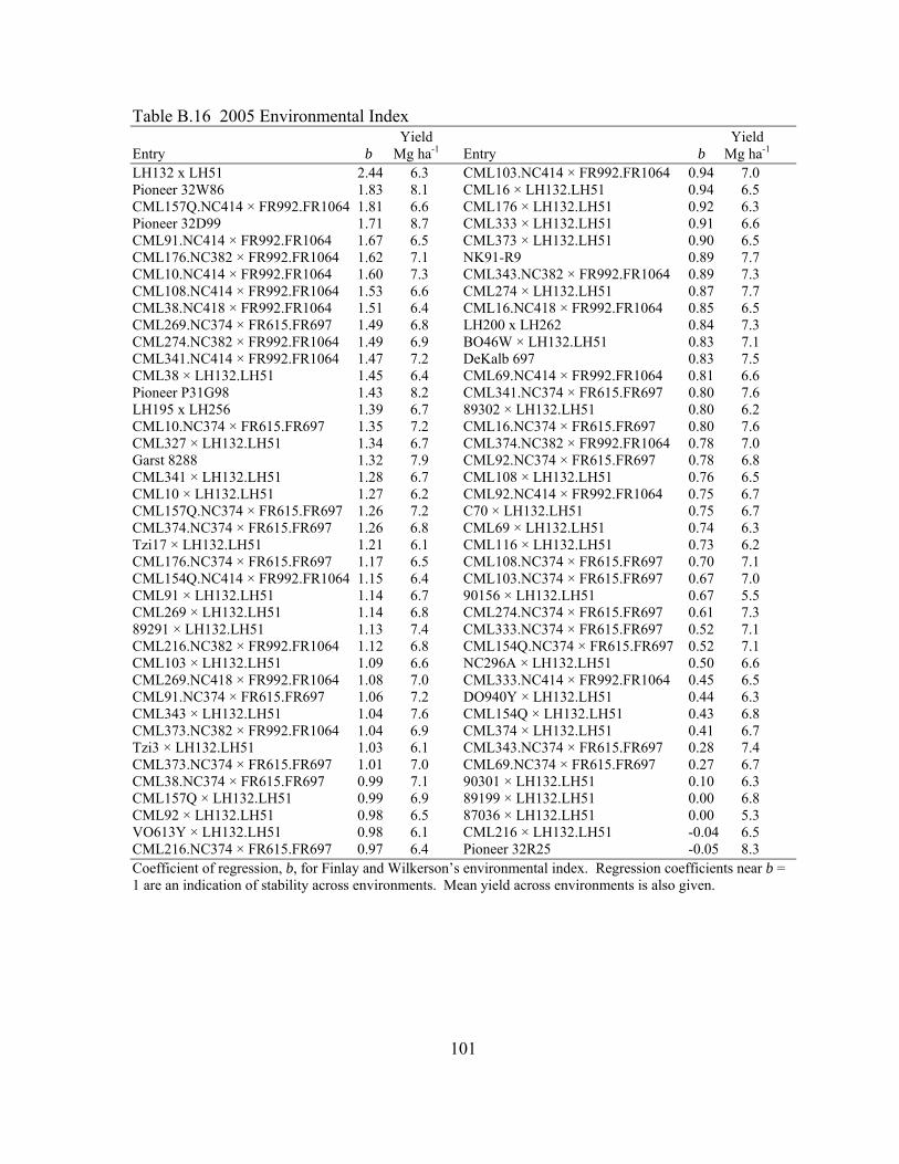
101
Table B.16 2005 Environmental Index Yield Yield Entry b Mg ha-1 Entry b Mg ha-1 LH132 x LH51 2.44 6.3 CML103.NC414 × FR992.FR1064 0.94 7.0 Pioneer 32W86 1.83 8.1 CML16 × LH132.LH51 0.94 6.5 CML157Q.NC414 × FR992.FR1064 1.81 6.6 CML176 × LH132.LH51 0.92 6.3 Pioneer 32D99 1.71 8.7 CML333 × LH132.LH51 0.91 6.6 CML91.NC414 × FR992.FR1064 1.67 6.5 CML373 × LH132.LH51 0.90 6.5 CML176.NC382 × FR992.FR1064 1.62 7.1 NK91-R9 0.89 7.7 CML10.NC414 × FR992.FR1064 1.60 7.3 CML343.NC382 × FR992.FR1064 0.89 7.3 CML108.NC414 × FR992.FR1064 1.53 6.6 CML274 × LH132.LH51 0.87 7.7 CML38.NC418 × FR992.FR1064 1.51 6.4 CML16.NC418 × FR992.FR1064 0.85 6.5 CML269.NC374 × FR615.FR697 1.49 6.8 LH200 x LH262 0.84 7.3 CML274.NC382 × FR992.FR1064 1.49 6.9 BO46W × LH132.LH51 0.83 7.1 CML341.NC414 × FR992.FR1064 1.47 7.2 DeKalb 697 0.83 7.5 CML38 × LH132.LH51 1.45 6.4 CML69.NC414 × FR992.FR1064 0.81 6.6 Pioneer P31G98 1.43 8.2 CML341.NC374 × FR615.FR697 0.80 7.6 LH195 x LH256 1.39 6.7 89302 × LH132.LH51 0.80 6.2 CML10.NC374 × FR615.FR697 1.35 7.2 CML16.NC374 × FR615.FR697 0.80 7.6 CML327 × LH132.LH51 1.34 6.7 CML374.NC382 × FR992.FR1064 0.78 7.0 Garst 8288 1.32 7.9 CML92.NC374 × FR615.FR697 0.78 6.8 CML341 × LH132.LH51 1.28 6.7 CML108 × LH132.LH51 0.76 6.5 CML10 × LH132.LH51 1.27 6.2 CML92.NC414 × FR992.FR1064 0.75 6.7 CML157Q.NC374 × FR615.FR697 1.26 7.2 C70 × LH132.LH51 0.75 6.7 CML374.NC374 × FR615.FR697 1.26 6.8 CML69 × LH132.LH51 0.74 6.3 Tzi17 × LH132.LH51 1.21 6.1 CML116 × LH132.LH51 0.73 6.2 CML176.NC374 × FR615.FR697 1.17 6.5 CML108.NC374 × FR615.FR697 0.70 7.1 CML154Q.NC414 × FR992.FR1064 1.15 6.4 CML103.NC374 × FR615.FR697 0.67 7.0 CML91 × LH132.LH51 1.14 6.7 90156 × LH132.LH51 0.67 5.5 CML269 × LH132.LH51 1.14 6.8 CML274.NC374 × FR615.FR697 0.61 7.3 89291 × LH132.LH51 1.13 7.4 CML333.NC374 × FR615.FR697 0.52 7.1 CML216.NC382 × FR992.FR1064 1.12 6.8 CML154Q.NC374 × FR615.FR697 0.52 7.1 CML103 × LH132.LH51 1.09 6.6 NC296A × LH132.LH51 0.50 6.6 CML269.NC418 × FR992.FR1064 1.08 7.0 CML333.NC414 × FR992.FR1064 0.45 6.5 CML91.NC374 × FR615.FR697 1.06 7.2 DO940Y × LH132.LH51 0.44 6.3 CML343 × LH132.LH51 1.04 7.6 CML154Q × LH132.LH51 0.43 6.8 CML373.NC382 × FR992.FR1064 1.04 6.9 CML374 × LH132.LH51 0.41 6.7 Tzi3 × LH132.LH51 1.03 6.1 CML343.NC374 × FR615.FR697 0.28 7.4 CML373.NC374 × FR615.FR697 1.01 7.0 CML69.NC374 × FR615.FR697 0.27 6.7 CML38.NC374 × FR615.FR697 0.99 7.1 90301 × LH132.LH51 0.10 6.3 CML157Q × LH132.LH51 0.99 6.9 89199 × LH132.LH51 0.00 6.8 CML92 × LH132.LH51 0.98 6.5 87036 × LH132.LH51 0.00 5.3 VO613Y × LH132.LH51 0.98 6.1 CML216 × LH132.LH51 -0.04 6.5 CML216.NC374 × FR615.FR697 0.97 6.4 Pioneer 32R25 -0.05 8.3 Coefficient of regression, b, for Finlay and Wilkerson’s environmental index. Regression coefficients near b = 1 are an indication of stability across environments. Mean yield across environments is also given.
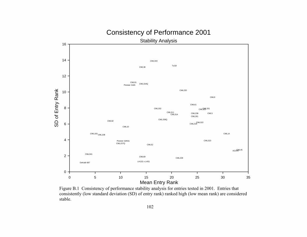
Consistency of Performance 2001Stability Analysis
Mean Entry Rank0 5 10 15 20 25 30 35
SD
of E
ntry
Ran
k
0
2
4
6
8
10
12
14
16
A214N
CML10
CML103 CML108 CML14
CML154Q
CML157Q
CML158Q
CML218
CML220
CML228
CML238CML261
CML311CML314
CML321
CML322
CML323
CML331CML332
CML333
CML341
CML38
CML45
CML5
CML52
CML61
CML69
CML9
CML91
CML92
DeKalb 687 LH132 x LH51
Pioneer 3165
Pioneer 32K61
Tzi18
Figure B.1 Consistency of performance stability analysis for entries tested in 2001. Entries that consistently (low standard deviation (SD) of entry rank) ranked high (low mean rank) are considered stable.
102
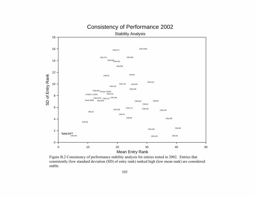
Consistency of Performance 2002Stability Analysis
Mean Entry Rank0 10 20 30 40 50
SD o
f Ent
ry R
ank
0
2
4
6
8
10
12
14
16
18
CML10
CML103
CML108
CML142CML144
CML145
CML150
CML154Q
CML157Q
CML159
CML16
CML161CML173
CML176 CML184
CML186
CML193
CML216
CML223
CML255
CML269
CML273
CML274
CML285
CML295
CML319
CML329
CML333
CML341
CML38
CML40
CML48
CML52
CML56
CML69
CML91
CML92
DeKalb 697
Garst 8288
LH200 x LH262Pioneer 32K61
Pioneer 31G98
Figure B.2 Consistency of performance stability analysis for entries tested in 2002. Entries that consistently (low standard deviation (SD) of entry rank) ranked high (low mean rank) are considered stable.
103
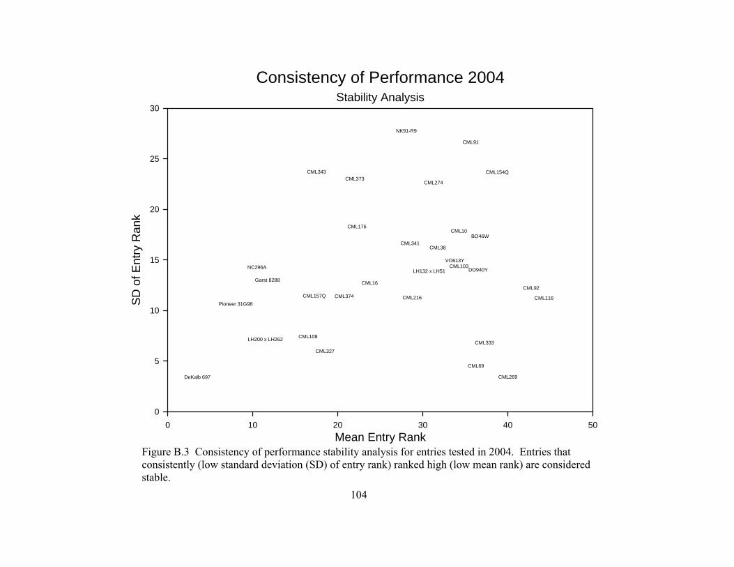
Consistency of Performance 2004Stability Analysis
Mean Entry Rank0 10 20 30 40 50
SD o
f Ent
ry R
ank
0
5
10
15
20
25
30
BO46WCML10
CML103
CML108
CML116
CML154Q
CML157Q
CML16
CML176
CML216
CML269
CML274
CML327
CML333
CML341
CML343CML373
CML374
CML38
CML69
CML91
CML92
DO940Y
DeKalb 697
Garst 8288
LH132 x LH51
LH200 x LH262
NC296A
NK91-R9
Pioneer 31G98
VO613Y
Figure B.3 Consistency of performance stability analysis for entries tested in 2004. Entries that consistently (low standard deviation (SD) of entry rank) ranked high (low mean rank) are considered stable.
104
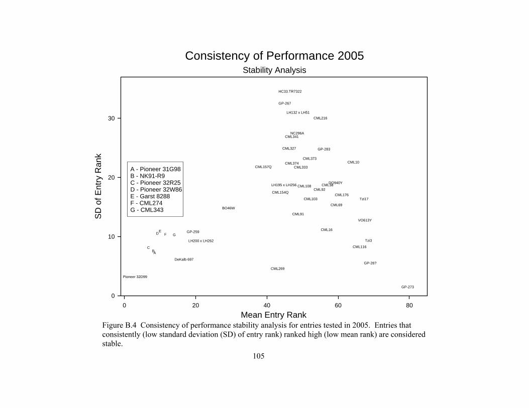
Consistency of Performance 2005Stability Analysis
Mean Entry Rank0 20 40 60 80
SD
of E
ntry
Ran
k
0
10
20
30
BO46W
CML10
CML103
CML108
CML116
CML154Q
CML157Q
CML16
CML176
CML216
CML269
F
CML327
CML333
CML341
G
CML373CML374
CML38
CML69
CML91
CML92
DO940Y
DeKalb 697
GP-259
GP-267
GP-26?
GP-273
GP-283
E
HC33.TR7322
LH132 x LH51
LH195 x LH256
LH200 x LH262
NC296A
B
Pioneer 32D99
C
D
A
Tzi17
Tzi3
VO613Y
A - Pioneer 31G98B - NK91-R9C - Pioneer 32R25D - Pioneer 32W86E - Garst 8288F - CML274G - CML343
Figure B.4 Consistency of performance stability analysis for entries tested in 2005. Entries that consistently (low standard deviation (SD) of entry rank) ranked high (low mean rank) are considered stable.
105
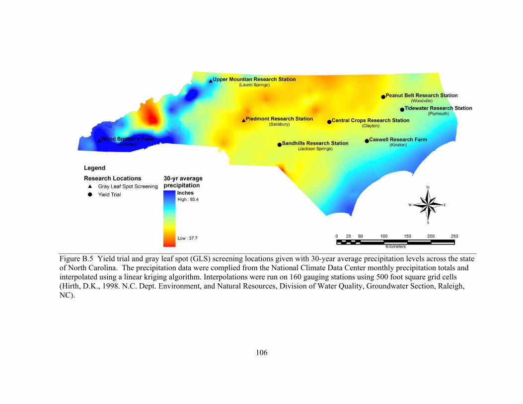
Figure B.5 Yield trial and gray leaf spot (GLS) screening locations given with 30-year average precipitation levels across the state of North Carolina. The precipitation data were complied from the National Climate Data Center monthly precipitation totals and interpolated using a linear kriging algorithm. Interpolations were run on 160 gauging stations using 500 foot square grid cells (Hirth, D.K., 1998. N.C. Dept. Environment, and Natural Resources, Division of Water Quality, Groundwater Section, Raleigh, NC).
106
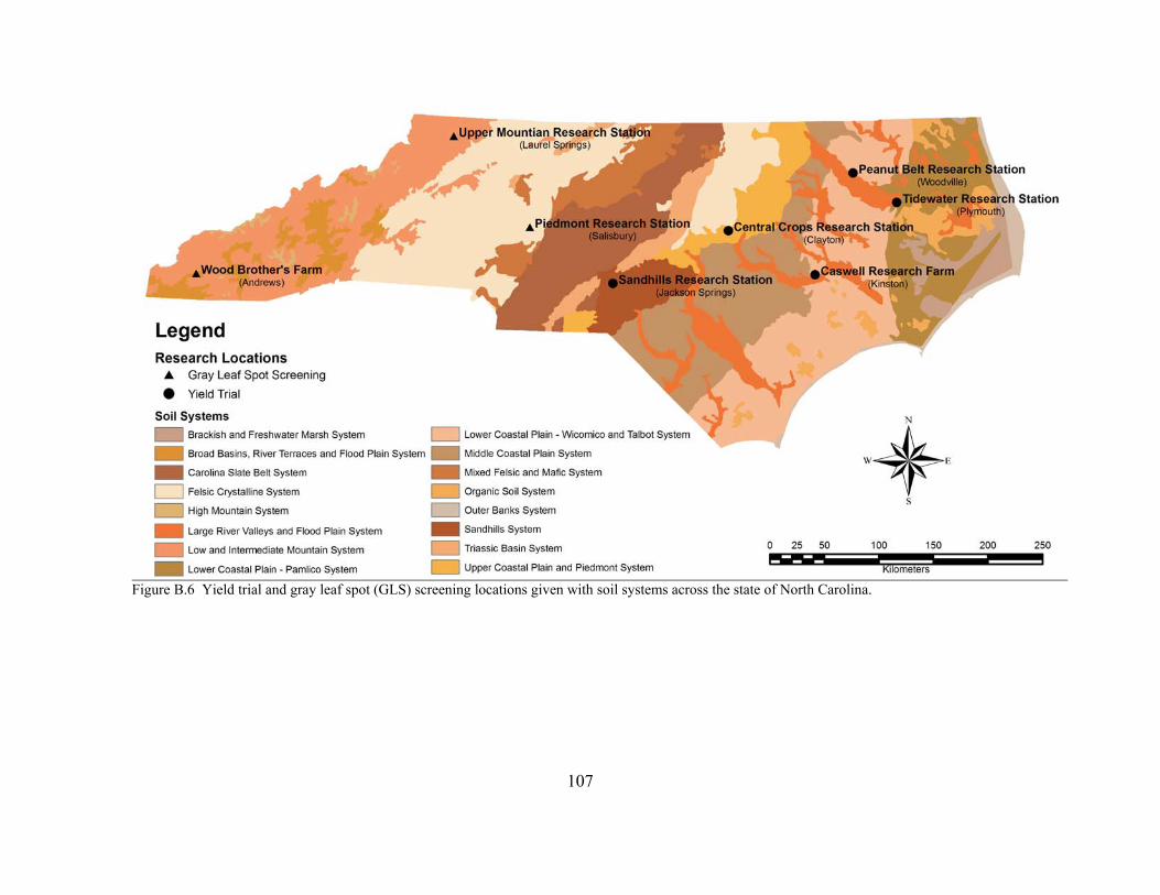
107
Figure B.6 Yield trial and gray leaf spot (GLS) screening locations given with soil systems across the state of North Carolina.

108
– APPENDIX C –
Supporting Material for Chapter IV
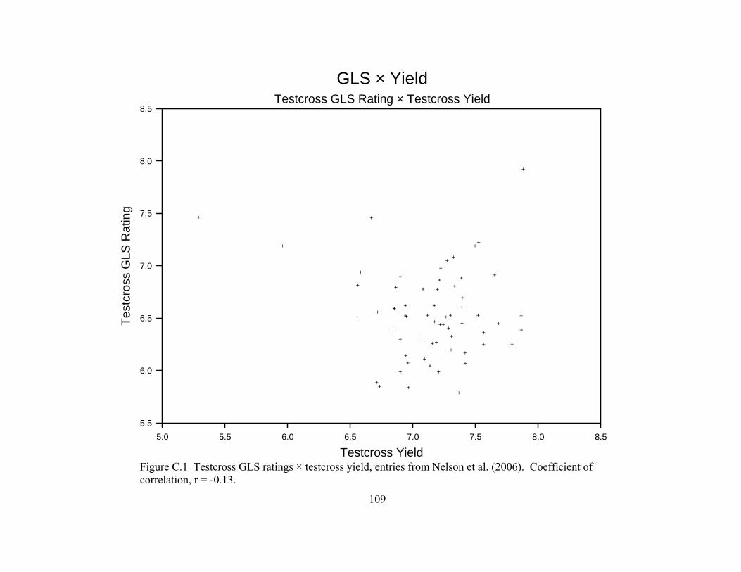
Testcross Yield5.0 5.5 6.0 6.5 7.0 7.5 8.0 8.5
Test
cros
s G
LS R
atin
g
5.5
6.0
6.5
7.0
7.5
8.0
8.5
+
+
+
+
+
+
+
+
+
+ +
++
+
+
+
+
+
+
+
+
+
+
+ +
++
+
++
+
+
+
+
+
+
+
+
+
++
+
+
+ +
+
+
+
+
+
+
+
+
+
+++
+
+
+
+
++
GLS × YieldTestcross GLS Rating × Testcross Yield
Figure C.1 Testcross GLS ratings × testcross yield, entries from Nelson et al. (2006). Coefficient of correlation, r = -0.13.
109
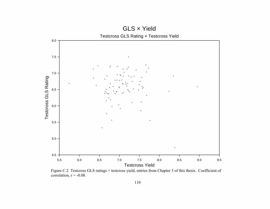
110
GLS × YieldTestcross GLS Rating × Testcross Yield
Testcross Yield5.5 6.0 6.5 7.0 7.5 8.0 8.5 9.0 9.5
Test
cros
s G
LS R
atin
g
4.5
5.0
5.5
6.0
6.5
7.0
7.5
8.0
++
+
++
+
+
+
+
+
+
+
+
+
+
+
+
+
+
+
+
+ +
+
+
+
+
+
+ +
++
+
+
+
+
+
+
+
+
+
+
+
+
++
+
+
+
+
+
++
+
+
+
+
++
+
+
+
+
+
++
+
+
+
+
+
+ +
+
+
+
++
+
+
+
+ +
Figure C.2 Testcross GLS ratings × testcross yield, entries from Chapter 3 of this thesis. Coefficient of correlation, r = -0.08.
111
– Appendix D –
Common and Southern Rust Evaluation Exotic Inbreds
Occasionally, conditions in North Carolina are conducive to infestations of the maize foliar
diseases common rust, caused by the fungus Puccinia sorghi, and southern rust, caused by
the fungus Puccinia polysora. In 2000, common rust occurred at Laurel Springs, NC, a gray
leaf spot screening location, and in 2003 southern rust occurred at Salisbury, NC, also a gray
leaf spot screening locations (Appendix B, Figures B.5 and B.6). In both instances a single
disease rating was taken for the respective diseases. Ratings were taken on a 1-9 scale, 1
being fully susceptible and 9 being fully resistant. Data for common rust ratings on 30
experimental inbreds and one check are provided in Table D.1 and data for southern rust
ratings on 44 experimental inbreds and four checks are provided in Table D.2.
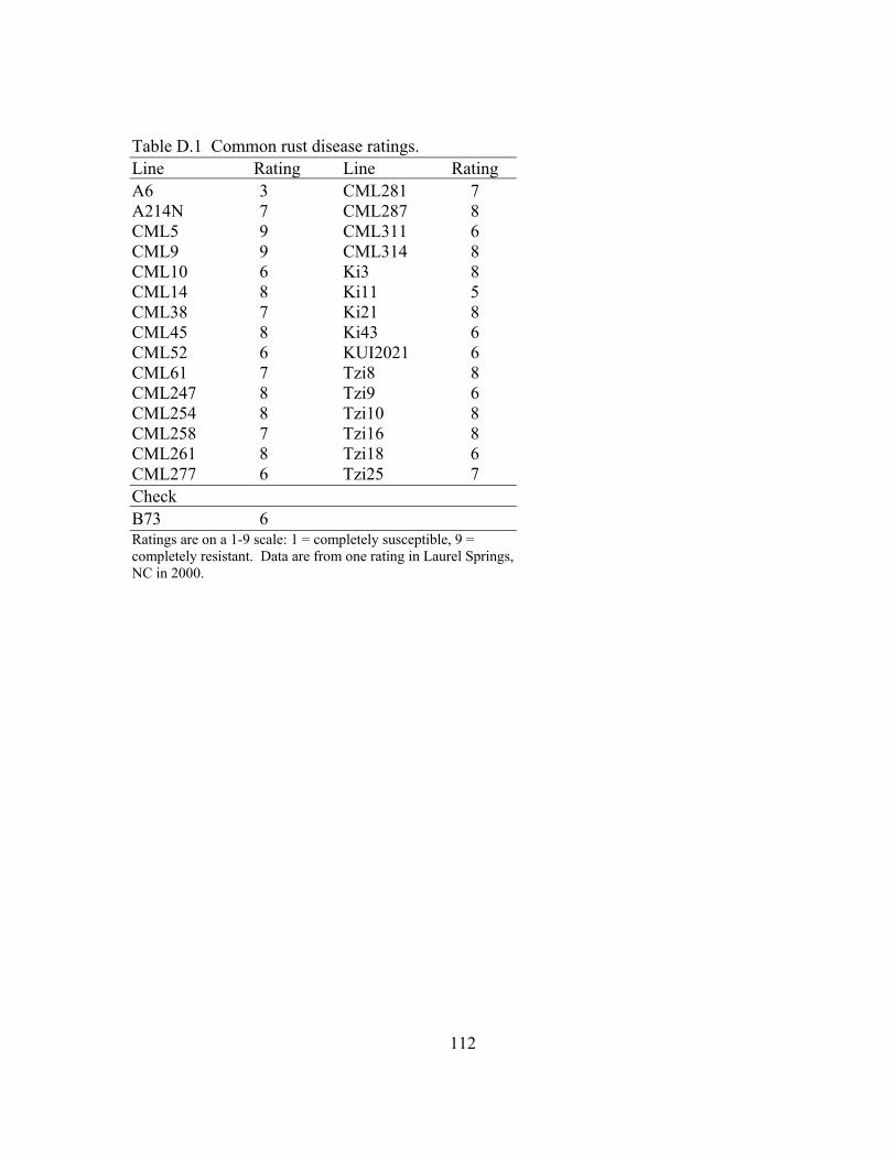
112
Table D.1 Common rust disease ratings. Line Rating Line Rating A6 3 CML281 7 A214N 7 CML287 8 CML5 9 CML311 6 CML9 9 CML314 8 CML10 6 Ki3 8 CML14 8 Ki11 5 CML38 7 Ki21 8 CML45 8 Ki43 6 CML52 6 KUI2021 6 CML61 7 Tzi8 8 CML247 8 Tzi9 6 CML254 8 Tzi10 8 CML258 7 Tzi16 8 CML261 8 Tzi18 6 CML277 6 Tzi25 7 Check B73 6 Ratings are on a 1-9 scale: 1 = completely susceptible, 9 = completely resistant. Data are from one rating in Laurel Springs, NC in 2000.
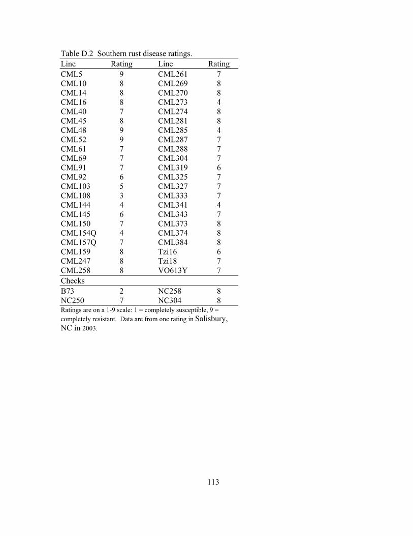
113
Table D.2 Southern rust disease ratings. Line Rating Line Rating CML5 9 CML261 7 CML10 8 CML269 8 CML14 8 CML270 8 CML16 8 CML273 4 CML40 7 CML274 8 CML45 8 CML281 8 CML48 9 CML285 4 CML52 9 CML287 7 CML61 7 CML288 7 CML69 7 CML304 7 CML91 7 CML319 6 CML92 6 CML325 7 CML103 5 CML327 7 CML108 3 CML333 7 CML144 4 CML341 4 CML145 6 CML343 7 CML150 7 CML373 8 CML154Q 4 CML374 8 CML157Q 7 CML384 8 CML159 8 Tzi16 6 CML247 8 Tzi18 7 CML258 8 VO613Y 7 Checks B73 2 NC258 8 NC250 7 NC304 8 Ratings are on a 1-9 scale: 1 = completely susceptible, 9 = completely resistant. Data are from one rating in Salisbury, NC in 2003.
![Construction of the third generation Zea mays haplotype map · domesticated Zea mays varieties [1]. Since then, more maize lines have been sequenced by the international research](https://img.pdfslide.us/doc/110x75/5e98d8e4c1f1f22e3e6b6c3f/construction-of-the-third-generation-zea-mays-haplotype-map-domesticated-zea-mays.jpg)
![Phenotyping of Hybrid Maize (Zea mays L.) at Seedling ...Oriza sativa), and maize (Zea mays), which provide over 50% of human calo-ries, are predicted to decrease [4]. It provides](https://img.pdfslide.us/doc/110x75/5ea6c60aa3205b46545f968a/phenotyping-of-hybrid-maize-zea-mays-l-at-seedling-oriza-sativa-and-maize.jpg)