Embed Size (px)
Citation preview

1
15.053 February 3, 2005
A brief review of Linear Algebra
Another LP formulation, and
Math Programming and Radiation Therapy

2
Review of Linear Algebra
Some elementary facts about vectors and matrices.The Gauss-Jordan method for solving systems of equations.Bases and basic solutions and pivoting.
Note: you are not expected to know 18.06, but will be expected to know about solving systems of equations.

3
Elementary Facts about Vectors
⎡ ⎤⎣ ⎦1 2 3 4v = v v v v is called a row vector.
⎡ ⎤⎢ ⎥⎢ ⎥=⎢ ⎥⎢ ⎥⎣ ⎦
1
2
3
4
t
vv
vvv
The transpose of v is a column vector.
[ ]1 2 3 4w w w w w= is another row vector.
The inner product of vectors v and w is given by:1 1 2 2 3 3 4 4
tv w vw v w v w v w v w= = + + +

4
Matrix Multiplication
=( )ijA a =( )ijB b = = ×( )ijC c A B
Suppose that A has n columns and B has n rows.
1=∑= k kjn
ikji a bc

5
Multiplying Matrices
Let C = (cij) = A × B. Then cij is the inner product of row i of A and column j of B.
⎡ ⎤⎢ ⎥= ⎢ ⎥⎢ ⎥⎣ ⎦
21 22 23
11 12 13
31 32 33
a a aA
aa
a aa a
⎡ ⎤⎢ ⎥= ⎢ ⎥⎢ ⎥⎣ ⎦
13
23
3
11 12
21 22
31 32 3
b bB b
b
bbb
bb
For example, what is c23?
= + +23 21 13 22 23 23 33c a b a b a b
6
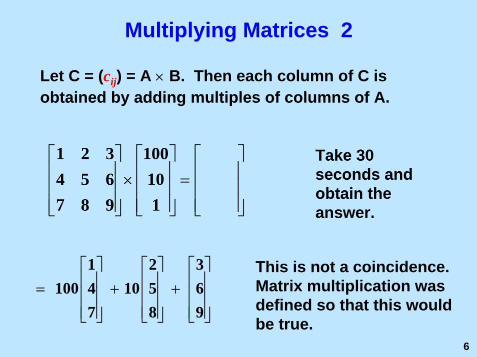
Multiplying Matrices 2
Let C = (cij) = A × B. Then each column of C is obtained by adding multiples of columns of A.
⎡ ⎤ ⎡ ⎤ ⎡ ⎤⎢ ⎥ ⎢ ⎥ ⎢ ⎥× =⎢ ⎥ ⎢ ⎥ ⎢ ⎥⎢ ⎥ ⎢ ⎥ ⎢ ⎥⎣ ⎦ ⎣ ⎦ ⎣ ⎦
1 2 3 1004 5 6 107 8 9 1
Take 30 seconds and obtain the answer.
⎡ ⎤ ⎡ ⎤ ⎡ ⎤⎢ ⎥ ⎢ ⎥ ⎢ ⎥= + +⎢ ⎥ ⎢ ⎥ ⎢ ⎥⎢ ⎥ ⎢ ⎥ ⎢ ⎥⎣ ⎦ ⎣ ⎦ ⎣ ⎦
1 2 3100 4 10 5 6
7 8 9
This is not a coincidence. Matrix multiplication was defined so that this would be true.

7
Multiplying Matrices 3
Let C = (cij) = A × B. Then each row of C is obtained by adding multiples of rows of A.
[ ] [ ]⎡ ⎤⎢ ⎥× =⎢ ⎥⎢ ⎥⎣ ⎦
1 2 3100 10 1 4 5 6
7 8 9 Take 30 seconds and obtain the answer.
[ ] [ ] [ ]= + +100 1 2 3 10 4 5 6 7 8 9
Matrix Premultiplication ⇔ Adding multiples of rows.
Elementary Facts about Solving Equations
1
2
3
xxxx
⎡ ⎤⎢ ⎥⎢ ⎥⎢ ⎥⎣ ⎦
=
3×12×1
06
b⎡ ⎤
= ⎢ ⎥⎣ ⎦
1 2 42 1 1
A⎡ ⎤
= ⎢ ⎥−⎣ ⎦2×3
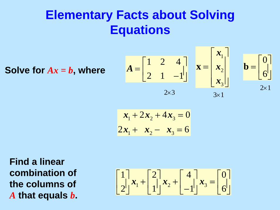
Solve for Ax = b, where
1 2 3
1 2 3
2 4 02 6
x x xx x x+ + =
+ − =
Find a linear combination of the columns of A that equals b.
1 2 3
1 2 4 02 1 1 6
x x x⎡ ⎤ ⎡ ⎤ ⎡ ⎤ ⎡ ⎤
+ + =⎢ ⎥ ⎢ ⎥ ⎢ ⎥ ⎢ ⎥−⎣ ⎦ ⎣ ⎦ ⎣ ⎦ ⎣ ⎦

9
Solving a System of Equations
x1 x2 x3 x4
1 2 4 1 = 02 1 -1 -1 = 6-1 1 2 2 = -3
To solve a system of equations, use Gauss-Jordan elimination.

10
To solve the system of equations:
1
2
-1
2
1
1
4
-1
2
1
-1
2
x1 x2 x3 x4
=
=
=
0
6
-3
G-J Animation

11
The fundamental operation: pivotinga special case of an elementary row operation (ero)
b1
b2
b3
=
=
=
a12
a22
a32
a14
a24
a34
a11
a21
a31
a13
a23
a33
x1 x2 x3 x4
Pivot on a23

12
Pivot on a23
x1 x2 x3 x4
a12
a22
a32
a14
a24
a34
a11
a21
a31
a13
a23
a33
1a21/a23
b1=
=
=
b2
b3
Take two minutes to fill in the other coefficients for constraint 2 and constraint 1 after the pivot.

13
Jordan Canonical Form for an m x n matrix
-1
1
2
1
0
00
1
0
-1
1
0
=
=
=
1
0
0 0
1
-1
x2x1 x3 x4
-1
1
0
x4
There are m columns that have been transformed into unit vectors, one for each row. The variables in these columns are called “basic.” The remaining variable(s) are called non-basic.

14
Jordan Canonical Form for an m x n matrix
x2x1 x3 x4
1
0
00
1
0
-1
1
0 -1
1
2=
=
=
1
0
0 0
1
-1
In the “basic solution”, the non-basic variables are set to 0.
The basic solution is: x1 = 2, x2 = 1, x3 = -1 x4 = 0

15
There is an easily determined solution for every choice of non-basic variables.
-1
1
2
1
0
00
1
0
-1
1
0
=
=
=
1
0
0 0
1
-1
x2x1 x3 x4Suppose we set x4 = 2.2
Equation 1 becomes: x1 – 2 = 2. So x1 = 4.
If we set x4 = 2, we get x1 = 4, x2 = -1, x3 = -1 x4 = 2.

16
Another Jordan Canonical Form
1
1
0
-1
1
0
4
-2
3
=
=
=
0
0
-2
3
-31 0 -1
0 0 3
0 1 1
x2x1 x3 x4
1
Take 60 seconds and answer the following questions.
What are the “basic” variables?
What is the basic solution?
What is the solution if the non-basic variable is set to 2?

17
The pigskin problem (from Practical Management Science)
Pigskin company makes footballs
All data below is for 1000s of footballs
Forecast demand for next 6 months
– 10, 15, 30, 35, 25 and 10
Current inventory of footballs: 5
Determine the production levels and inventory levels over the next six months
– meet demand at minimum cost
– satisfy constraints

18
The pigskin problem (continued)
Max Production capacity: 30 per month
Max Storage capacity: 10 per month
Production Cost per football for next 6 months:
– $12.50, $12.55, $12.70, $12.80, $12.85, $12.95
Holding cost: $.60 per football per month
With your partner: write an LP to describe the problem, but only write variables and constraints for the next 3 months.

19
On the formulation
Choose decision variables.
– Let xj = the number of footballs produced in month j (in 1000s)
– Let yj = the number of footballs held in inventory from month j to month j + 1. (in 1000s)
– y0 = 5
Then write the constraints and the objective.

20
The formulation
Minimize
subject to
y0 = 5
0 <= yj <= 10 for j = 1, 2, 3
0 <= xj <= 30 for j = 1, 2, 3
Pigskin Spreadsheet

21
Math Programming and Radiation TherapyAn important application area for optimization
Lecture notes originally from 15.094
Thanks to Rob Freund who developed these notes with help from Peng Sun
22
Math Programming and Radiation Therapy
High doses of radiation (energy/unit mass) can kill cells and/or prevent them from growing and dividing
– True for cancer cells and normal cells
Radiation is attractive because the repair mechanisms for cancer cells is less efficient than for normal cells
Radiation Short Clip

23
Radiation Therapy OverviewRecent advances in radiation therapy now make it possible to– map the cancerous region in greater detail– aim a larger number of different beamlets with greater
specificityThis has spawned the new field of tomotherapy“Optimizing the Delivery of Radiation Therapy to Cancer patients,” by Shepard, Ferris, Olivera, and Mackie, SIAM Review, Vol 41, pp 721-744, 1999.Also see http://www.tomotherapy.com/

24
Conventional Radiotherapy
Relative Intensity of Dose Delivered

25
Conventional Radiotherapy
Relative Intensity of Dose Delivered

26
Conventional RadiotherapyIn conventional radiotherapy
– 3 to 7 beams of radiation
– radiation oncologist and physicist work together to determine a set of beam angles and beam intensities
– determined by manual “trial-and-error” process

27
Goal: maximize the dose to the tumor while minimizing dose to the critical area
Critical Area
Tumor area
With a small number of beams, it is difficult to achieve these goals.

28
Recent AdvancesMore accurate map of tumor area
– CT -- Computed Tomography
– MRI -- Magnetic Resonance Imaging
More accurate delivery of radiation
– IMRT: Intensity Modulated Radiation Therapy
– Tomotherapy

29
Tomotherapy: a diagram

30
Radiation Therapy: Problem Statement
For a given tumor and given critical areas
For a given set of possible beamlet origins and angles
Determine the weight of each beamlet such that:
– dosage over the tumor area will be at least a target level γL .
– dosage over the critical area will be at most a target level γU.

31
Display of radiation levels

32
Linear Programming ModelFirst, discretize the space
– Divide up region into a 2D (or 3D) grid of pixels

33
More on the LP
Create the beamlet data for each of p = 1, ..., n possible beamlets.
Dp is the matrix of unit doses delivered by beam p.
pijD = unit dose
delivered to pixel (i, j) by beamlet p

34
Linear Program
Decision variables w = (w1, ..., wp)
wp = intensity weight assigned to beamlet pfor p = 1 to n;
Dij = dosage delivered to pixel (i, j)
1==∑n p
ij ij ppD D w

35
An LP model
took 4 minutes to solve.∑ ( , ) iji j
Dminimize
1==∑n p
ij ij ppD D w
γ≥ ∈ for ( , )ij LD i j T
γ≤ ∈ for ( , )ij UD i j C
0≥ for allpw p
In an example reported in the paper, there were more than 63,000 variables, and more than 94,000 constraints (excluding upper/lower bounds)
36
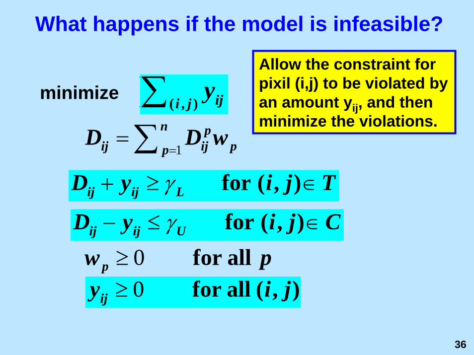
What happens if the model is infeasible?
1==∑n p
ij ij ppD D w
Allow the constraint for pixil (i,j) to be violated by an amount yij, and then minimize the violations.
∑ ( , ) iji jD∑ ( , ) iji jyminimize
γ≥ ∈ for ( , )ij LD i j Tγ+ ≥ ∈ for ( , )ij ij LD y i j T
γ≤ ∈ for ( , )ij UD i j Cγ− ≤ ∈ for ( , )ij ij U i jD y C0≥ for allpw p0≥ for all ( , )ijy i j

37
An even better model
1==∑n p
ij ij ppD D w
minimize ∑ ( , ) iji jD∑ ( , ) iji jy( )2
∑ ( , ) iji jy minimize the sum of
squared violations.
γ≥ ∈ for ( , )ij LD i j Tγ+ ≥ ∈ for ( , )ij ij LD y i j T
γ≤ ∈ for ( , )ij UD i j CLeast squaresγ− ≤ ∈ for ( , )ij ij U i jD y C
0≥ for allpw p0≥ for all ( , )ijy i j
This is a nonlinear program (NLP). This one can be solved efficiently.

38
Optimal Solution for the LP

39
An Optimal Solution to an NLP

40
Is that the end of the story on modeling?
Other issues:
– Delivering the radiation doses quicker by setting the multi-leaf collimators optimally.
– trying to keep average radiation levels low over part of the critical region.
– how do we trade off the doses to the critical area with doses to the tumor?

41
The 2003 Edelman Prize for OR/MS Practice
Winner: Canadian Pacific Railway "Perfecting the Scheduled Railroad: Model-Driven Operating Plan Development."
– Previous operation: Waits for enough cargo before trains leave.
– Their goal: move towards a fixed schedule.
– Used OR techniques to determine the best fixed schedule
– Savings in cost: $170 million.
42
The 2003 Edelman Prize for OR/MS Practice
2nd place. UPS and MIT "Planning the UPS Air Network."
Goal: develop an optimize service network design for express package delivery. – minimal-cost aircraft routes– fleet assignments – allocation of packages to routes – 17,000 origin-destination pairs, 160 aircraft
Savings from optimization: $275 million

43
SummaryGauss-Jordan solving of equations and other background in linear algebra
Optimization in Radiation Delivery
Modeling in practice is an art form. It requires finding the right simplifications of reality for a given situation.
The 2003 Edelman prize competition.

44
15.053
Animation of the Gauss-Jordan Elimination Algorithm

45
Solving a System of Equations
x1 x2 x3 x41 2 4 1 = 02 1 -1 -1 = 6-1 1 2 2 = -3
To solve a system of equations, use Gauss-Jordan elimination.

46
To solve the system of equations:
x1 x2 x3 x4
1
2
-1
2
1
1
4
-1
2
1
-1
2
=
=
=
0
6
-3

47
Pivot on the element in row 1 column 1
x1 x2 x3 x4
1
2
-1
2
1
1
4
-1
2
1
-1
2
=
=
=
=
=
=
0
6
-3
0
0
-3
3
-9
6
-3
3
1 2 4 1 0
6
-3
Subtract 2 times constraint 1 from constraint 2. Add constraint 1 to constraint 3.

48
Pivot on the element in Row 2, Column 2
x1 x2 x3 x4
1
2
-1
2
1
1
4
-1
2
1
-1
2
=
=
=
=
=
=
0
6
-3
0
0
-3
3
-9
6
-3
3
2 4 1 0
6
-3
Take two minutes and carry out the “pivot” operation.

49
Pivot on the element in Row 2, Column 2
x1 x2 x3 x4
=
=
=
1
0
0
2
-3
3
4
-9
6
1
-3
3
1 13
0 -2 -1
0 -3 0
1
0
0
0
6
-3
-2
3
4
Divide constraint 2 by -3. Subtract multiples of constraint 2 from constraints 1 and 3.

50
Pivot on the element in Row 3, Column 3
x1 x2 x3 x4
0
1
0
-1
1
0
4
-2
3
=
=
=
1
0
0
-2
3
-3
0 -1 201
0 1 110
1 0 -100
Divide constraint 3 by -3. Add multiples of constraint 3 to constraints 1 and 2.
Suppose x4 = 0. What are x1, x2, x3?

51
The fundamental operation: pivoting
x1 x2 x3 x4
b1
b2
b3
=
=
=
a12
a22
a32
a14
a24
a34
a11
a21
a31
a13
a23
a33
=
=
=
Pivot on a23

52
Pivot on a23 ⎯a11 =a11 –a13(a21/a23)
x1 x2 x3 x4
b1
b2
b3
=
=
=
a12
a22
a32
a14
a24
a34
a11
a21
a31
a13
a23
a33
What will be the next coefficient of b1? a32? of aij for i ≠2?
=
=
=
a22/a23 a24/a23a21/a23 1
0
0
⎯a11
b2/a23