Assessing the Value of Clean Air in a

Developing Country: A Hedonic Price Analysis of the Jakarta Housing Market, Indonesia

Arief Anshory Yusuf

Budy P. Resosudarmo

Australian National University Economics and Environment Network Working Paper

EEN0601

21 February 2006

Assessing the Value of Clean Air in a Developing Country:

A Hedonic Price Analysis of the Jakarta Housing Market, Indonesia

Arief Anshory Yusuf Budy P. Resosudarmo

Economics Division Research School of Pacific and Asian Studies

The Australian National University

Correspondent address: budy.resosudarmo@anu.edu.au

1

Assessing the Value of Clean Air in a Developing Country: A Hedonic Price Analysis of the Jakarta Housing Market,

Indonesia

Abstract

This paper is motivated by the common argument that clean air is a luxury good and has

much less or even no value in a less developed country. It applies a hedonic property value

analysis, a method commonly used to infer the value of clean air in developed countries,

using a combination of data on house values and their characteristics from the Indonesian

Family Life Survey, and data of the ambient level of six different pollutants in Jakarta,

Indonesia. The result suggests that air quality may affect property value in Jakarta, indicating

a preference toward environmental amenities. Moreover, this study is one of the first hedonic

studies that may potentially give comparable estimates of the value of clean air in developing

countries.

JEL Classification: R22; H40; Q21; C14

Keywords: Hedonic Prices, Air Pollution, Indonesia

2

1. Introduction

Since the early 1990s, urban air pollution, particularly in mega cities of developing countries,

has been recognized as one of the world’s major environmental concerns (UNEP and WHO,

1992; WRI et al., 1998). A decade later, nevertheless, various tables showing several

environmental quality indicators, available in the World Development Indicators 2004, still

indicate that cases of severe urban air quality in developing countries continue to occur

(World Bank, 2004). Clearly, there are serious difficulties involved in effectively

implementing air pollution policies in developing countries. The most common argument for

this failure is that clean air is a luxury good and most people in developing countries hardly

know what it means to consume it. Therefore, the value of an air pollution policy becomes

insignificant for them, and they do not place an air pollution policy among their top

priorities.1 This argument needs to be tested. Hence, the goal of this paper is to elicit

whether people in developing countries care about and so value cleaner air.

Jakarta is used as the case study since data on the levels of air pollutant for this city is

available and the pollutants have reached an alarming level. In the last few years in

Indonesia, there has been growing concern, particularly among NGOs, that urban air quality

has been at a disturbing level (MEB, 2002). The worst air quality is certainly in Jakarta, the

largest city in Indonesia with a population of approximately 25 million, a population density

of 14 thousand people/km2, and around 1.5 million cars and 2.5 million motorcycles daily on

the streets. In various places in Jakarta in 1998, the levels of total suspended particles and

nitrogen dioxide reached approximately 270 µg/m3 and 148 µg/m3, respectively, while the

WHO allowable levels for these pollutants are 90 µg/m3 and 50 µg/m3. From these figures,

Resosudarmo and Napitupulu (2004) estimated that the total health cost associated with

pollutants in Jakarta was approximately 180 million US$ or approximately one percent of

Jakarta’s GDP or approximately as much as the total revenue of the Jakarta government for

that year.

Since 2001, various NGOs have been able to lobby the Jakarta government to initiate

a new clean air program to improve air quality in the city significantly. The new program

mostly targets the reduction of air pollution from vehicles, and hence includes activities such

1 The argument that environmental goods are luxuries has been used to support the hypothesis that air pollution increases with income when income is low, but decreases when income is high. This is supported empirically by the so-called Environmental Kuznet Curve.

3

as the elimination of lead in gasoline, the implementation of an emission standard,

improvement in public transport management and the adoption of strict emission inspection

of vehicles (MEB, 2002). By 2003, lead was eliminated from the gasoline sold in Jakarta.

However, the progress with other activities has been very slow, so that there is still a high

level of air pollutants other than lead.

The valuation of environmental amenities, including clean air, is a complex area of

research, because most environmental goods are non-marketed, hence their appropriate value

cannot be easily identified. There are basically two broad approaches to environmental

valuation. The first is the direct approach that attempts to elicit preferences directly by the

use of a survey and experimental techniques such as the Contingent Valuation Method

(CVM). The second is the indirect approach that seeks to elicit preferences from people’s

observed behaviour in the market; i.e. the preference of environmental amenities is revealed

indirectly, when an individual purchases a marketed good (for example a house) related to

the environmental good in question. Hedonic analysis is one technique in the category of

indirect approaches (Pearce et al., 1995). The fact that it is observed people’s actual

behaviour in a real market that infers their valuation of the related commodities is among the

advantages of the hedonic method. It is, in contrast, the hypothetical situation that could lead

to much bias that constrains the direct approach to valuation such as CVM from producing

reliable inference on people’s valuation.2

This paper chooses to implement a hedonic analysis on property value to elicit the

value of clean air. This choice is interesting for the following reasons. First, whereas most

studies of this kind are for developed countries (Smith and Huang, 1995, Boyle and Kiel,

2001), this paper implements the technique for a developing country. The second motivation

is that spatial data on levels of six different air pollutants, and data on property values along

with their characteristics, are available for Jakarta. This data makes it possible for this paper

to combine a hedonic analysis and a spatial analysis. Only a few studies have used this

combined technique (Kim et al., 2003).

This paper is divided into 5 sections. Section 1 discusses the background and

motivation of this research. Section 2 presents the theoretical background of hedonic

property value analysis and a short review of its relevant applications to air quality and

2 See Arrow et al, 1993 for a comprehensive discussion of the strength and weaknesses of the contingent valuation method.

4

property value. Section 3 describes the estimation methodology and data. Section 4 provides

a discussion of its result and its implications. Section 5 is the conclusion.

2. Hedonic Property Value Studies and Air Quality

Air quality is an attribute of a house the variability of which may affect the

willingness to pay (WTP) for the house as a whole. Hence, the structure of housing rents and

prices will reflect these differentials. By using data on rent/prices of different properties,

hedonic price analysis can in principle identify the contribution air quality makes to the value

of the traded good, the house. This identifies an implicit or shadow price of these attributes,

which in turn can be used to calculate willingness to pay for the non-marketed goods, namely

the improvement of air quality. The method commonly used to implement this approach is

the hedonic technique pioneered by Griliches (1971) and formalised by Rosen (1974).

Hedonic property value analysis, however, suffers from theoretical and empirical

problems. From the theoretical point of view, some strong assumptions, which are the

foundations of this theory, are considered unrealistic by certain critics. The market clearing

condition, for example, requires that the housing market is in equilibrium. It also requires a

sufficiently wide variety of housing models available such that every household is in

equilibrium. Many consider this strong assumption as the reason why applying this

framework to an under-developed housing market in developing countries is hardly feasible.

However, in Jakarta metropolitan area, which is the Indonesian capital, its housing and

property market is relatively developed, especially compared to rural area of Indonesia.

Yusuf and Koundouri (2005), conclude, for example, that housing market in Indonesian

urban area is relatively developed and suitable for hedonic analysis, compared to rural area,

as indicated by comparing goodness of fit of urban and rural hedonic price estimation.

There are also many practical problems in empirical works of hedonic property value

analysis. These include the definition and measurement of the dependent variable of the

hedonic price functions, its explanatory variables, correct or best functional forms, and

identification problems. One problem, considered common in empirical analysis, is the

presence of multicollinearity, since there could be too many explanatory variables in the

hedonic price equations.

There have been an enormous number of hedonic property value studies in an attempt

to find out whether air quality is associated with property value, particularly in developed

5

countries. Smith and Huang (1995) provided a formal summary of over 50 studies on

hedonic analysis for US cities during the period of 1967–1988. They used a comprehensive

meta–analysis of the hedonic property value model to address the issue of whether the

housing market can value air quality which is measured by the concentration of particulate

matter. This review concluded that the MWTP for one unit reduction of particulate matter

lies between zero and US$ 98.

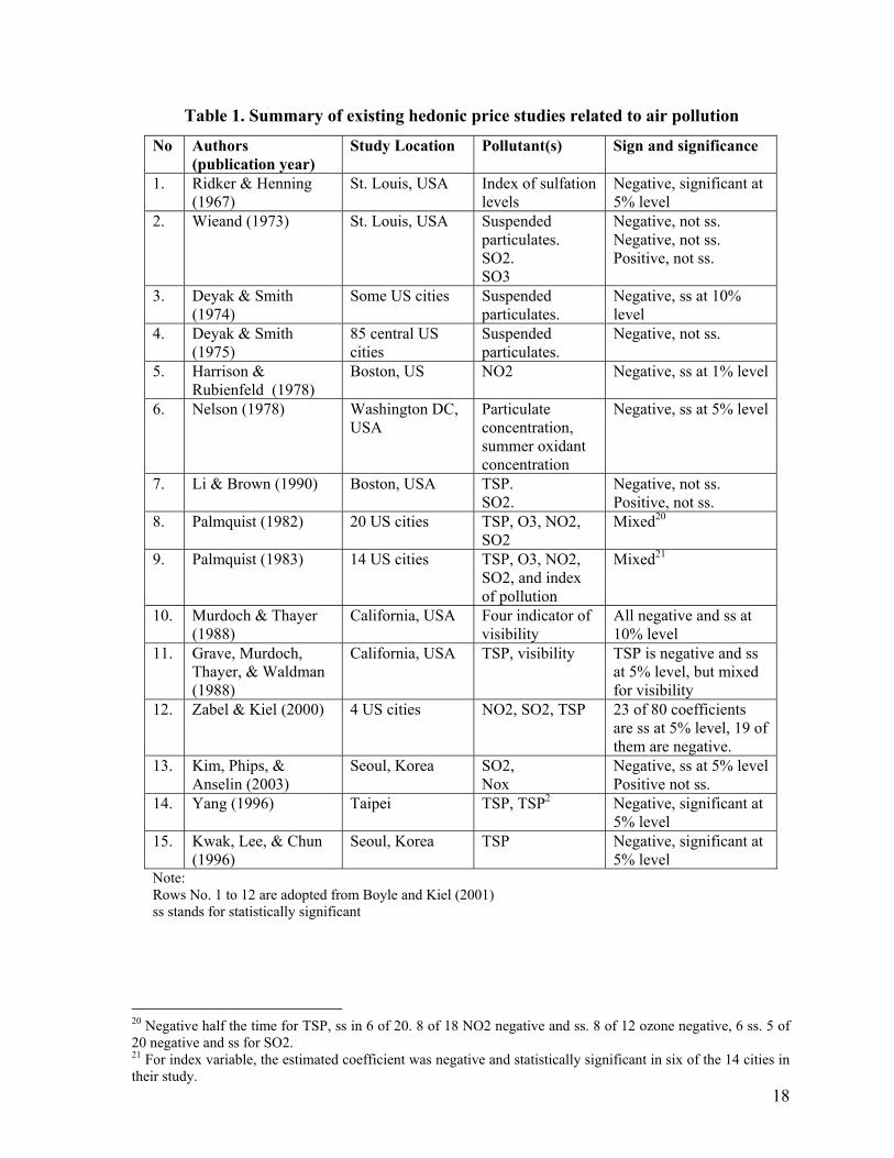
Boyle and Kiel (2001) is another study providing a more recent review of 12 hedonic

studies for US cities. Table 1 (rows 1 to 12) presents the 12 studies surveyed by Boyle and

Kiel (2001). The conclusion of this study is mixed; i.e. although most cases suggest that air

pollution negatively and significantly affects property value, implying that people are willing

to pay for air quality improvement, there are other cases showing that the effect might be not

significant.

From an intensive literature study, it reveals that the implementation of hedonic

housing value analysis in North America and Europe are relatively abundant. For outside

North America and Europe, works on this subject are relatively very few; for example, there

are two studies for Seoul-Korea and one for Taipei-Taiwan. (See the last three rows in Table

1.) Furthermore, despite the importance and relevance of knowing whether or not and by

how much people in poorer countries value air quality, hedonic studies to infer the value of

air quality in the developing world are rare3. It seems that the availability of consistent air

pollution data is one of the main reasons. This study, then, will be among the few

applications of hedonic price analysis to study the value of clean air in developing countries.

3. Methodologies and Data

3.1. Estimation methodology

Since the theoretical underpinnings of hedonic analysis do not suggest a specific

functional form, choosing the best functional form is merely an empirical question. To this

end we employ a flexible functional form using the Box-Cox transformation method4. The

hedonic equation to be estimated is,

∑ ∑ +++=i j jjii xxy εγβα λλ

2)(

1)( (1)

3 To our knowledge. 4 The Box-Cox model is the most common functional form used in hedonic price analysis (see Cropper et al, 1999).

6

where

λ

λλ 1)( −= yy ;

λ

λλ 11)(

1−

= ii

xx (2)

with α, β, and γ representing vectors of coefficients to be estimated, y the monthly rent of the

house, x1i vector of variables to be transformed (i.e., size of the house, number of rooms,

distance to district centre, and ambient level of 6 different types of pollution) using the

formula in equation (2), x2j the vector of other variables (dummy variables and variables that

are not strictly positive and thus could not be transformed using the formula in equation (2)),

and λ is the parameter of the transformation (functional form is linear when λ = 1 and log-

linear when λ = 0), and ε is the error term. The model will be estimated using the Maximum

Likelihood method (Greene, 2000, pp.444–453 and Haab and McConnel, 2002 pp. 254–256).

Since many more recent hedonic price studies suggest that in a cross-sectional

hedonic price analysis the value of a property in one location may also be affected by

property values in other locations5, such as in its neighbouring area, this paper will also

check for the presence of this spatial effect. This spatial analysis will be summarised and

reported in the appendix.

3.2. Data

Data for the dependent variable (monthly house rent), structural characteristics, and

neighbourhood characteristics are taken from the Indonesian Family Life Survey (IFLS)

1997–98, whereas data for air pollution variables are from a study conducted by the ADB

(Syahril et al., 2003). The ADB study measured and reported concentrations of air pollution

in Jakarta in 1998, almost at the same time as the survey of IFLS ended. The IFLS6 is a

continuing longitudinal socio-economic survey, the first wave of which was conducted in

1993 (IFLS1). The second wave (IFLS2) was conducted from 1997 to 1998. The sampling

scheme used for Indonesia overall was stratified into provinces, and then randomly sampled

within provinces. Thirteen of the nation's twenty-six provinces were selected with the aim of

capturing the cultural and socio-economic diversity of Indonesia. Within each of the thirteen

5 Dubin (1988, 1992) was one of the first researchers to introduce treatments for the presence of spatial effect in a hedonic analysis work. Since then it has been applied in many more recent studies such as, among others, Bockstael and Bell (1997), Geoghegan et al. (1997), LeSage (1997), Legget and Bockstael (2000), Gawande and Jenkin-Smith (2001), Kim et al. (2003), and Bransington and Hite (2004). 6 The dataset is freely downloadable from http://www.rand.org/labor/FLS/IFLS.

7

provinces, enumeration areas (EAs) — an area of a village — were randomly selected, over-

sampling urban EAs and EAs in smaller provinces to facilitate urban-rural and Javanese-non-

Javanese comparisons. Finally, within each selected EA households were randomly selected,

producing around 7,000 households for Indonesia as a whole. For this paper, a sub-sample of

470 observations from Jakarta province is used. This sub-sample represents the population of

Jakarta, because of the nature of the provincial stratification of this sampling7.

Variables of the hedonic equations that are selected are those commonly used in the

literature of hedonic property value analysis. The selection of variables also considers the

data availability. Monthly house rental (in Rupiahs) is used for the dependent variable in the

hedonic equation. In hedonic studies, either the price or the rent of the house is used for

dependent variables. Since the price or the value of the house is essentially the present value

of its stream of rents, the choice between the two is not important. Structural characteristics

that are included are the size of the house (in square meters), the number of rooms, material

used for walls, roofs, and floors, and water source availability. These structural

characteristics are expected to be positively associated with property value. To represent the

quality of the neighbourhood, some variables which are aggregated at the village level (or

kelurahan level in the case of Jakarta)8 are selected. The unemployment rate (which is

expected to be negatively associated with house value) and the percentage of people in the

village with a university education (expected to be positively associated with property value)

are proxies for the general quality of the neighbourhood. Accessibility of public transport

(expected to be positively associated with house price) and distance to the centre of Jakarta

(expected to be negatively associated with house price) attempt to measure the house's

accessibility to employment.

Air quality is measured by the annual average ambient air concentration of six

different pollutants i.e. PM10 (small particulates), SO2 (sulphur dioxide), CO (carbon

monoxide), NOx (nitrogen oxide), THC (total hydro carbon), and Pb (lead). The first two of

these pollutants mainly come from fixed sources, whereas the rest mainly come from mobile

sources. This paper will not include the six of them together in one equation for the following

reasons. First, this paper is trying to measure is people perception on air quality in general. 7 The number of samples from Jakarta is proportional to the population of Jakarta, not a result of random sampling across Indonesia. 8 Note that Jakarta is a city consisting of five districts (or kotamadya). Each kotamadya consists of several sub-districts or kecamatan. There is a total of 53 sub-districts in Jakarta. Each kecamatan consists of several villages or kelurahan.

8

Most people simply do not aware of what type of pollutants is involved. Hence, including all

pollutants is less sensible since, for most people, each of them may just a proxy of the same

things; i.e. dirty air. Therefore, finding any of those pollution variables negatively significant

is most likely enough to indicate that people do not like dirty air in general. Second,

including all of the six pollutants will create a multicollinearity problem. It is very likely that

indicators of different pollution are correlated to each other, simply because they may come

from the same sources (mostly the burning of fossil fuels). This problem may reduce the

precision of the estimates9. For this reason this paper treats air pollutants individually, and

therefore there will be six different specifications for six different pollutants.10.

The ADB (Syahril et al., 2003) measured and reported the annual average

concentration of air pollution, aggregated for 53 sub-districts (or kecamatan) of Jakarta. They

were measured based on the combination of the direct measurement at the air quality

monitoring station in Jakarta, and the (environmental) model which takes into account

industry level, number/type of vehicles, traffic, wind direction, and meteorological data11.

Concerns exist regarding the accuracy of this air pollution data. Nevertheless, since

no study of this hedonic type has been undertaken for developing countries, the exercise in

this paper, despite this limitation, may enrich the existing literature by providing some

evidence in the context of developing countries, and will be improved upon by future

availability of more reliable data.

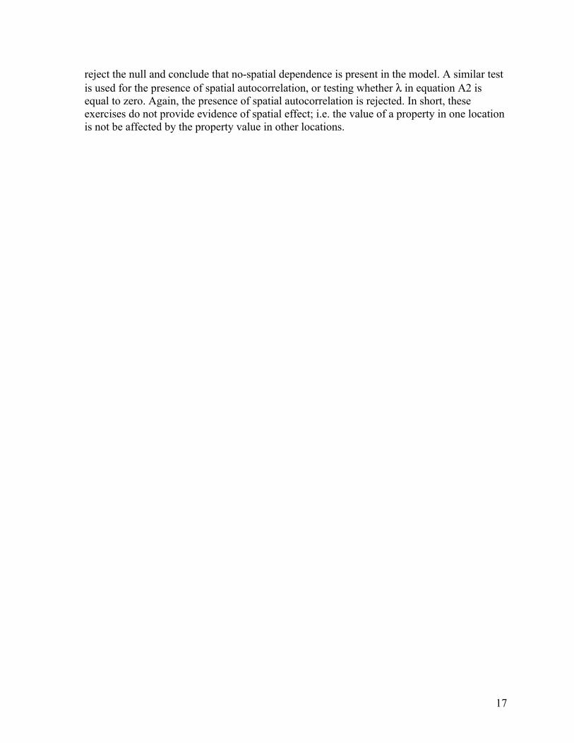
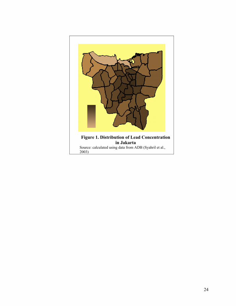
Figure 1 below shows how one of the pollutants (lead) is distributed among sub-

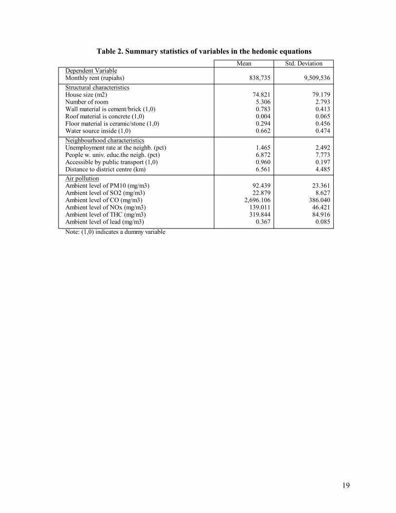
districts in Jakarta (the darker the colour, the higher the lead concentration in the area). Table

2 provides a detailed description and summary of statistics of all variables used in the

hedonic equation.

Combining the IFLS and air pollution data sets, however, raise one problem.. Since

pollution is measured and reported for every sub-district, which is not really accurate because

pollution does not recognize administrative boundaries, a pollution level of one house may

9 Cross-correlation among those pollutants is very high, and later on, estimation results that include all six pollutants create severe multicollinearity as indicated by the value of the Variance Inflating Factor of more than 100 or even 800. 10 We also tried to use a combination of one pollutant from a mobile source, and one from a fixed source, since people may know how close they are to sources of pollution. Because there are two distinct sources of pollution i.e. stationary/fixed sources people will take into account two different types of information in deciding where they live. For example, they will try to avoid living near factories and areas with heavy traffic. However, the result using this specification does not change any conclusion, but the report is available upon request. 11 For more details on the discussion of air pollution data, readers may refer to the ADB publication (Syahril et al, 2003), which is available on the ADB web site.

9

not necessarily better be represented by the pollution of the district where it is located. The

house could be located in the center (where it is appropriate to use its respective district

pollution) or close to the border (where it is more appropriate to use the pollution of its

neighbour). In short, measurement error problem, to some extent, is unavoidable. To

minimize the problem, a simple average of the pollution level around this neighbourhood is

calculated. A house located in sub-district A will assume the average air quality of sub-

district A and its surrounding sub-districts. Intuitively, this averaging technique is analogous

to moving average or seasonal adjustment method commonly used for time series data, but

now in the spatial context. Seasonal adjustment, through averaging process, will implicitly

reduce the effect of measurement error (Hausman and Watson, 1983, p. 1)

4. Results and discussion

The estimation results presented in Table 3 suggest that the linearity and log-linearity of the

dependent variable is rejected.12 Parameter λ in the Box-Cox model is estimated as ranging

from around -0.1570 to -0.1595, and it is strongly significant at the 1 percent level across the

six specifications. This may suggest that, in terms of the goodness-of-fit (likelihood value),

the flexible functional form is preferred.

House structural characteristics and neighbourhood qualities are strongly associated

with house values. In all specifications, house structural characteristics; i.e. house size,

number of rooms, wall and floor materials, are all positively associated (as expected) with

house value and are significant at the 5 percent level. Only roof material is significant at the

10 percent level.

Three out of four neighbourhood characteristics conform to expectation, and are

significant at the 5 percent level. The unemployment rate within the neighbourhood is

negative and is significantly associated with house value, whereas the percentage of people

with a university education, and accessibility of public transport are positively associated

with house values. Both are significant at the 5 percent level.

Distance to the centre of Jakarta, however, is not statistically associated with house

value; it is not significant at a conventional level, and two reasons may account for this.

First, distance to the centre of Jakarta may not be a good measure of accessibility to

12 Stata conducted automatic hypothesis testing for θ = -1, θ = 0; θ = 1. All tests conducted are rejected at the conventional level.

10

employment. The better measure may be distance to the centre of a district (or kotamadya in

the case of Jakarta13) where important business centres are located. The second reason is that

the accessibility of employment might have already been captured by accessibility of public

transport (which is positively significant).

All of the coefficients of pollution variables, except PM10, are now negative,

suggesting better air quality is associated with higher property value, and 3 out of 6 are

statistically significant (10% for SO2 and THC, and 5% for Lead). This result has quite a

straightforward implication i.e. it does not support the claim that people in developing

countries are not concerned with air quality. By calculating the marginal effect of a change in

1 unit of SO2, for example, it can be interpreted that marginal willingness to pay (MWTP) for

a reduction of SO2 concentration is around Rp. 448.25.14 Boyle and Kiel (2001 p.120) in

their survey of hedonic studies, report a few estimates of the dollar value of SO2

concentration as ranging from $58 to $328 per µg/m3. To make it comparable, the MWTP

from this study is capitalised15 and converted into 1997 US$, resulting in as much as $28 per

µg/m3. Although certainly this is still far below the value people in a developed country are

willing to pay, it is a good indication that people in Jakarta may in fact be aware and also be

willing to pay to avoid living in a polluted area.

Some caveats, however, are worth noting. First, the estimate of MWTP is imprecise,

since the coefficient of most of the pollution variables is only marginally significant.

Secondly, a difficulty in interpretation may arise when trying to use the estimates to infer the

MWTP for reduction in every pollutant due to the high correlation among different types of

pollution variables.

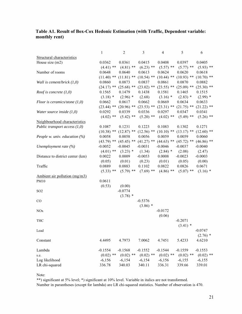
Two other final concerns in terms of the quality of the estimation are the possibility

of omitted variable bias due to the possibility that it is congestion level, not air quality, that is

captured by the pollution variables, and the potential presence of spatial effects. To deal with

the former, data on traffic16 (i.e. number of vehicles passing through every area) is used to

proxy the level of congestion. The model is re-estimated adding the traffic variable as one of

13 Jakarta is a province, and district is a town or locality. 14 Marginal effect is calculated as a derivative of the rent in the hedonic price function with respect to its explanatory variable e.g. SO2, and evaluated around the mean of all the explanatory variables. The report on the marginal effect of all the variables (including their standard errors and confidence interval) is available upon request. 15 Using a 5% discount rate and a 25 year period. Most of the hedonic studies report MWTP as a change in the asset value of the house (Smith and Huang, 1995). 16 Available in Syahril et al (2003).

11

the explanatory variables, and the result is shown in Table A1 in the appendix. The result

suggests no sign of inconsistency in the estimators, since there is no significant change in the

value of the coefficients. It even turns out that CO now becomes significant at a level of

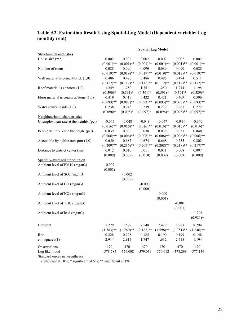
10%, adding one more pollution variable as significant. Spatial analysis is also performed by

estimating a spatial dependence and spatial error model, and is discussed in more detail in the

appendix. The result does not suggest the presence of any spatial effect17.

5. Conclusion

This paper is an attempt to elicit the value residents of Jakarta place on cleaner air and to

contribute to the debate as to whether or not most people in developing countries, in this case

in Jakarta, care about the quality of air in their neighbourhood, and as a result, whether or not

they place value on a policy to improve air quality. The main assumption in this paper is that

if people do care about air quality in the area where they live, it must be an important

attribute of their houses. Hence, a hedonic property value analysis can be used to infer

indirectly people’s preference concerning air quality, from the price they pay for their

houses.

It must be admitted that the main weakness of this paper is the data on air pollution.

However, the very existence of this data is progress in a way, since its non-existence in other

developing countries has prevented similar hedonic studies. Firstly, the measurement of air

quality in Jakarta as conducted by Syahril et al. (2003) is a relatively new activity. There has

not been any debate as to whether or not the approached taken by Syahril et al. (2003) can

really produce reliable data on spatial air quality. Secondly, the unit of the air pollution data

is an annual average concentration of an air pollutant covering a sub-district area. This

information might not accurately represent the severity of air quality in several spots in a

sub-district for a particular season, which is actually an important factor determining housing

value in such spots. Meanwhile for several other spots, an annual average concentration of an

air pollutant covering a sub-district area might overestimate the air quality around these

areas. The third, as already mentioned while describing the data set, is that several house

owners, particularly those on the periphery of a sub-district, might consider that the air

quality in the adjacent sub-district is the same as the quality of his/her neighbourhood; i.e. the

17 The positive sign of the coefficient of traffic, however, needs to be carefully interpreted. It may be argued that traffic not only represents the congestion level but also closeness to other city attractions. So the two effects may oppose each other, and the latter seems to be stronger.

12

definition of a neighbourhood for an individual might not coincide with the boundary of a

sub-district. The fourth is that the time periods when the IFLS household data and the data of

the air quality were collected do not exactly match.

Bearing in mind all these weaknesses, several points might be noted from the

empirical exercises in this paper. First, the empirical results indicate that air pollutants might

have a negative association with property value. In the cases of lead, total hydro carbon

(THC), SO2, and CO, the relationship is negative and significant. This finding, hence, does

not support the common argument that people in developing countries do not have a

preference for quality air.

Finally, the empirical result of this paper may also imply that any effort to reduce air

pollution in Jakarta, so long as it outweighs its appropriate financial cost can be welfare-

enhancing. This paper certainly supports the recent implementation of policy to phase out

lead from gasoline used in Jakarta. It remains a puzzle why efforts to reduce other air

pollutants do not progress smoothly in Jakarta. Further research on this topic would certainly

be valuable.

References

Anselin, Luc. (1988), Spatial Econometrics: Methods and Models. Boston: Kluwer

Academic.

Boyle, M. A., & Kiel, K. A. (2001). A survey of house price hedonic studies of the impact of

environmental externalities. Journal of Real Estate Literature, 9(2), 117-144.

Bransington D. M. and D. Hite (2004). Demand for environmental quality: a spatial hedonic

analysis. Regional Science and Urban Economics, article in press.

Chattopadhyay, S. (1999). Estimating the demand for air quality: New evidence based on the

Chicago housing market. Land Economics, 75(1), 22-38.

Cropper, M. L., Deck, L. B., & McConnell, K. E. (1999 [1988]). On the choice of functional

form for hedonic price functions. In M. Cropper (Ed.), Valuing environmental benefits:

Selected essays of Maureen cropper (pp. 306-313). New Horizons in Environmental

Economics. Cheltenham, U.K. and Northampton, Mass.: Elgar.

Dasgupta, P., & Maler, K. (1994). Poverty, institutions, and the environmental-resource

base. Washington, D.C.: World Bank.

13

Deyak, T. A., & Smith, V. K. (1974). Residential property values and air pollution: Some

new evidence. Quarterly Review of Economics and Business, 14(4), 93-100.

Dubin, R. A. (1992). Spatial autocorrelation and neighborhood quality. Regional Science and

Urban Economics, 22(3), 433-452.

Dubin, R. A. (1988). Estimation of regression coefficients in the presence of spatially auto-

correlated error terms. Review of Economics and Statistics, 70(3), 466-474.

Freeman, A. M. (1995), The measurement of environmental and resource values: theory and

method, Resource for the Future, New York.

Gawande, K., & Jenkins-Smith, H. (2001). Nuclear waste transport and residential property

values: Estimating the effects of perceived risks. Journal of Environmental Economics

and Management, 42(2), 207-233.

Geoghegan, J., Wainger, L. A., & Bockstael, N. E. (1997). Spatial landscape indices in a

hedonic framework: An ecological economics analysis using GIS. Ecological

Economics, 23(3), 251-264.

Greene, William H. (2000), Econometric Analysis, Prentice Hall International, London.

Griliches Z., ed. (1971), Price Indexes and Quality Change. Cambridge, Mass.: Harvard

University Press.

Haab, T. C., & McConnell, K. E. (2002). Valuing environmental and natural resources: The

econometrics of non-market valuation. and Northampton, Mass.: Elgar.

Harrison, D., Jr, & Rubinfeld, D. L. (1978). Hedonic housing prices and the demand for

clean air. Journal of Environmental Economics and Management, 5(1), 81-102.

Hausman, J. A., & Watson, M. W. (1983). Seasonal adjustment with measurement error

present. National Bureau of Economic Research, Inc, NBER Working Papers.

Kim, C. W., Phipps, T. T., & Anselin, L. (2003). Measuring the benefits of air quality

improvement: A spatial hedonic approach. Journal of Environmental Economics and

Management, 45(1), 24-39.

Kwak, S., Lee, G., & Chun, Y. (1996). Estimation of the benefit of air quality improvement:

An application of hedonic price technique in Seoul. In R. Mendelssohn, & D. Shaw

(Eds.), The economics of pollution control in the Asia pacific (pp. 171-181). New

Horizons in Environmental Economics series. Cheltenham, U.K. and Lyme, N.H.: Elgar;

distributed by American International Distribution Corporation, Williston, Vt.

14

Leggett, C. G., & Bockstael, N. E. (2000). Evidence of the effects of water quality on

residential land prices. Journal of Environmental Economics and Management, 39(2),

121-144.

LeSage, J. P. (1997). Regression analysis of spatial data. Journal of Regional Analysis and

Policy, 27(2), 83-94.

Li, M. M., & Brown, H. J. (1980). Micro-neighborhood externalities and hedonic housing

prices. Land Economics, 56(2), 125-141.

Mitra Emisi Bersih (MEB), 2002. Integrated Vehicle Emission Reduction Strategy for

Greater Jakarta. Menteri Negara Lingkungan Hidup, Jakarta.

Murdoch, J. C., & Thayer, M. A. (1988). Hedonic price estimation of variable urban air

quality. Journal of Environmental Economics and Management, 15(2), 143-146.

Nelson, J. P. (1978). Residential choice, hedonic prices, and the demand for urban air quality.

Journal of Urban Economics, 5(3), 357-369.

Palmquist, R. B. (1982). Measuring environmental effects on property values without

hedonic regressions. Journal of Urban Economics, 11(3), 333-347.

Resosudarmo, B.P. and L. Napitupulu, 2004, Health and Economic Impact of Air Pollution

in Jakarta, The Economic Record, 80(Special): S65-S75.

Pearce, D., Whittington, D, Georgiou, S,. and Moran, D. (1995), Economic Values and the

Environment in the Developing World, A Report to the United Nations Environment

Program, UNEP.

Ridker, R. G., & Henning, J. A. (1992 [1967]). The determinants of residential property

values with special reference to air pollution. In W. E. Oates ed (Ed.), The economics of

the environment (pp. 368-379). An Elgar Reference Collection. International Library of

Critical Writings in Economics, vol. 20. Aldershot, U.K.: Elgar; distributed in the U.S.

by Ashgate, Brookfield, Vt.

Rosen, S. (1974), `Hedonic prices and implicit markets: product differentiation in pure

competition', Journal of Political Economy, 82(1): 34-55.

Smith, V. K., & Deyak, T. A. (1975). Measuring the impact of air pollution on property

values. Journal of Regional Science, 15(3), 277-288.

Smith, V. K., & Huang, J. (1995). Can markets value air quality? A meta-analysis of hedonic

property value models. Journal of Political Economy, 103(1), 209-227.

15

Syahril, S., B.P. Resosudarmo, H.S. Tomo, 2003, Study on Air Quality in Jakarta, Indonesia:

Future Trends, Health Impacts, Economic Value and Policy Options. Report for the

Asian Development Bank, Manila.

The Economist, 1998, Development and The Environment, 19 March 1998 edition

Wieand, K. F. (1973). Air pollution and property values: A study of the st. louis area. Journal

of Regional Science, 13(1), 91-95.

Yang, C. (1996). Hedonic housing values and benefits of air quality improvement in Taipei.

In R. Mendelssohn, & D. Shaw eds (Eds.), The economics of pollution control in the

Asia pacific (pp. 150-170). New Horizons in Environmental Economics series.

Cheltenham, U.K. and Lyme, N.H.: Elgar; distributed by American International

Distribution Corporation, Williston, Vt.

Zabel, J. E., & Kiel, K. A. (2000). Estimating the demand for air quality in four U.S. cities.

Land Economics, 76(2), 174-194.

World Bank (1997), China 2020 : development challenges in the new century, World Bank,

Washington DC.

World Bank. (2000). Greening industry: New roles for communities, markets, and

governments. New York and Oxford: Oxford University Press.

Yusuf, Arief Anshory and Phoebe Koundouri (2005), "Willingness to Pay for Water and

Location Bias in Hedonic Price Analysis: Evidence from Indonesian Housing Market",

Environment and Development Economics, 10(6), 1-17.

16

Appendix: Spatial Analysis

More recently, many hedonic price studies suggest that in a cross-sectional hedonic price analysis, the value of a property in one location may also be affected by property values in other locations, such as in its neighbouring area. Ignoring this spatial effect or spatial dependence may cause the simple OLS estimation to be either inconsistent or inefficient (see Anselin, 1988 for text-book treatment of spatial econometrics). Here, the presence of this spatial effect will be tested and treatment procedures will be carried out if needed

In general, there are two classes of model developed to attenuate the problems of spatial effect, namely the spatial lag model and the spatial error model. In the spatial lag model, house price not only depends on its characteristics but also depends on the house price of its neighbours. The spatial lag model is an appropriate tool when capturing neighbourhood spillover effects. It assumes that the spatially weighted sum of neighbourhood housing prices (the spatial lag) enters as an explanatory variable in the specification of housing price formation, or εXβPWP ++= ~~ ρ (A1) Where ρ is spatial dependence parameter and W is an n× n standardized spatial weight matrix (where n is the number of observations). Spatial weight matrix, W, tells whether any pair of observations are neighbour. If, for example, house i and house j are neighbours then, wij = 1 and zero otherwise. Whether or not any pair of houses is neighbours is either determined by them sharing common borders (contiguity) or based on a certain distance between them18.

Spatial weight matrix is usually standardized, such that every row of the matrix is summed to 1. This enables us to interpret the spatial lag term in a spatial model as simply a spatially-weighted average of neighbouring house prices, for example,

∑ =++++= k

j jj xPwPwPwP1 16163132121 )( εβρ , where observation 2, 3, 6 are neighbours of

observation 1. The spatial lag model more or less resembles the AR model in time-series econometrics. However, unlike the AR model, OLS estimation in the presence of spatial dependence will be inconsistent, because of the endogeneity problem. The spatial lag model will be estimated using maximum likelihood estimation (see Anselin 1988, for detail MLE method). The spatial error model takes the following form εXβP +=~ ; uWεε += λ (A2) Where u now is the i.i.d error term, and λ is the spatial error parameter. The spatial error model resembles more or less the Moving Average model in time series econometrics, in which error of certain observations is affected by errors of other observation. The OLS estimation of spatial error model will be inefficient19 because it violates the assumption of the independence among disturbance term.

The result of estimating equation A1 and A5 can be seen in Tables A2 and A3 respectively. To test the existence of spatial dependence, this paper conducts a statistical test to see whether ρ in equation A1 (spatial dependence model) is equal to zero. With H0: ρ = 0, and Ha: ρ ≠ 0, the statistics follow χ2 distribution with 1 degree of freedom; this paper fails to 18 STATA can conveniently construct a spatial weight matrix based on certain distance. We used this method, alternatively, i.e. use distance as criteria to be neighbour. The choice of the distance band is constructed such that it represents as closely as possible that based on contiguity. Several different bands are constructed, but this does not affect the result. 19 See Anselin (1988) for more detail.

17

reject the null and conclude that no-spatial dependence is present in the model. A similar test is used for the presence of spatial autocorrelation, or testing whether λ in equation A2 is equal to zero. Again, the presence of spatial autocorrelation is rejected. In short, these exercises do not provide evidence of spatial effect; i.e. the value of a property in one location is not be affected by the property value in other locations.

18

Table 1. Summary of existing hedonic price studies related to air pollution

No Authors (publication year)

Study Location Pollutant(s) Sign and significance

1. Ridker & Henning (1967)

St. Louis, USA Index of sulfation levels

Negative, significant at 5% level

2. Wieand (1973) St. Louis, USA Suspended particulates. SO2. SO3

Negative, not ss. Negative, not ss. Positive, not ss.

3. Deyak & Smith (1974)

Some US cities Suspended particulates.

Negative, ss at 10% level

4. Deyak & Smith (1975)

85 central US cities

Suspended particulates.

Negative, not ss.

5. Harrison & Rubienfeld (1978)

Boston, US NO2 Negative, ss at 1% level

6. Nelson (1978) Washington DC, USA

Particulate concentration, summer oxidant concentration

Negative, ss at 5% level

7. Li & Brown (1990) Boston, USA TSP. SO2.

Negative, not ss. Positive, not ss.

8. Palmquist (1982) 20 US cities TSP, O3, NO2, SO2

Mixed20

9. Palmquist (1983) 14 US cities TSP, O3, NO2, SO2, and index of pollution

Mixed21

10. Murdoch & Thayer (1988)

California, USA Four indicator of visibility

All negative and ss at 10% level

11. Grave, Murdoch, Thayer, & Waldman (1988)

California, USA TSP, visibility TSP is negative and ss at 5% level, but mixed for visibility

12. Zabel & Kiel (2000) 4 US cities NO2, SO2, TSP 23 of 80 coefficients are ss at 5% level, 19 of them are negative.

13. Kim, Phips, & Anselin (2003)

Seoul, Korea SO2, Nox

Negative, ss at 5% level Positive not ss.

14. Yang (1996) Taipei TSP, TSP2 Negative, significant at 5% level

15. Kwak, Lee, & Chun (1996)

Seoul, Korea TSP Negative, significant at 5% level

Note: Rows No. 1 to 12 are adopted from Boyle and Kiel (2001) ss stands for statistically significant

20 Negative half the time for TSP, ss in 6 of 20. 8 of 18 NO2 negative and ss. 8 of 12 ozone negative, 6 ss. 5 of 20 negative and ss for SO2. 21 For index variable, the estimated coefficient was negative and statistically significant in six of the 14 cities in their study.

19

Table 2. Summary statistics of variables in the hedonic equations Mean Std. Deviation

Dependent VariableMonthly rent (rupiahs) 838,735 9,509,536 Structural characteristicsHouse size (m2) 74.821 79.179 Number of room 5.306 2.793 Wall material is cement/brick (1,0) 0.783 0.413 Roof material is concrete (1,0) 0.004 0.065 Floor material is ceramic/stone (1,0) 0.294 0.456 Water source inside (1,0) 0.662 0.474 Neighbourhood characteristicsUnemployment rate at the neighb. (pct) 1.465 2.492 People w. univ. educ.the neigh. (pct) 6.872 7.773 Accessible by public transport (1,0) 0.960 0.197 Distance to district centre (km) 6.561 4.485 Air pollutionAmbient level of PM10 (mg/m3) 92.439 23.361 Ambient level of SO2 (mg/m3) 22.879 8.627 Ambient level of CO (mg/m3) 2,696.106 386.040 Ambient level of NOx (mg/m3) 139.011 46.421 Ambient level of THC (mg/m3) 319.844 84.916 Ambient level of lead (mg/m3) 0.367 0.085 Note: (1,0) indicates a dummy variable

20

Table 3. Result of Box-Cox Hedonic Estimation (Dependent variable: monthly rent)

1 2 3 4 5 6Structural characteristicsHouse size (m2) 0.0363 0.0333 0.0370 0.0370 0.0366 0.0383

(4.52) ** (4.25) ** (5.12) ** (4.77) ** (5.08) ** (5.47) **Number of rooms 0.0625 0.0629 0.0614 0.0621 0.0613 0.0610

(10.89) ** (11.93) ** (11.00) ** (10.84) ** (11.17) ** (10.84) **Wall is cement/brick (1,0) 0.0810 0.0813 0.0791 0.0810 0.0816 0.0845

(22.31) ** (23.68) ** (21.55) ** (22.10) ** (23.42) ** (24.39) **Roof is concrete (1,0) 0.1640 0.1548 0.1583 0.1640 0.1525 0.1541

(3.62) * (3.42) * (3.42) * (3.60) * (3.24) * (3.24) *Floor is ceramics/stone (1,0) 0.0672 0.0629 0.0671 0.0673 0.0640 0.0630

(24.99) ** (23.04) ** (25.35) ** (25.01) ** (23.49) ** (22.03) **Water source inside (1,0) 0.0302 0.0339 0.0323 0.0303 0.0351 0.0357

(4.44) ** (5.72) ** (5.02) ** (4.44) ** (5.95) ** (6.09) **Neighbourhood characteristicsPublic transport access (1,0) 0.0981 0.1101 0.1033 0.0983 0.1191 0.1236

(8.85) ** (11.00) ** (9.66) ** (8.85) ** (11.71) ** (12.47) **People w. univ. education (%) 0.0052 0.0051 0.0050 0.0053 0.0052 0.0055

(39.10) ** (40.07) ** (35.90) ** (39.99) ** (40.88) ** (43.75) **Unemployment rate (%) -0.0067 -0.0064 -0.0061 -0.0066 -0.0056 -0.0053

(7.34) ** (7.97) ** (6.72) ** (6.95) ** (5.62) ** (4.85) **Distance to district center (km) 0.0072 0.0070 0.0049 0.0069 0.0036 0.0037

(0.52) (0.53) (0.24) (0.46) (0.13) (0.14)Ambient air pollution (mg/m3)PM10 0.0060

(0.01)SO2 -0.0650

(2.80) *CO -0.2498

(0.98)NOx -0.0049

(0.01)THC -0.1968

(3.15) *Lead -0.0898

(4.41) **Constant 4.9275 5.0527 6.0606 4.9662 5.6452 4.8122

Lambda -0.1572 -0.1595 -0.1578 -0.1570 -0.1585 -0.1575s.e. (0.02) ** (0.02) ** (0.02) ** (0.02) ** (0.02) ** (0.02) **Log likelihood -6,159 -6,157 -6,158 -6,159 -6,157 -6,156LR chi-squared (11) 331.45 334.24 332.42 331.45 334.60 335.85

Note:**) significant at 5% level; *) significant at 10% level. Variable in italics are not transformed.Number in parantheses (except for lambda) are LR chi-squared statistics. Number of observation is 470.

21

Table A1. Result of Box-Cox Hedonic Estimation (with Traffic, Dependent variable: monthly rent)

1 2 3 4 5 6Structural characteristicsHouse size (m2) 0.0362 0.0361 0.0415 0.0408 0.0397 0.0405

(4.41) ** (4.81) ** (6.23) ** (5.57) ** (5.77) ** (5.93) **Number of rooms 0.0648 0.0640 0.0613 0.0624 0.0620 0.0618

(11.40) ** (11.81) ** (10.54) ** (10.44) ** (10.93) ** (10.70) **Wall is cement/brick (1,0) 0.0860 0.0873 0.0837 0.0861 0.0870 0.0882

(24.17) ** (25.68) ** (23.02) ** (23.55) ** (25.09) ** (25.30) **Roof is concrete (1,0) 0.1565 0.1479 0.1438 0.1581 0.1465 0.1515

(3.18) * (2.96) * (2.68) (3.16) * (2.83) * (2.99) *Floor is ceramics/stone (1,0) 0.0662 0.0617 0.0662 0.0669 0.0634 0.0633

(23.44) ** (20.96) ** (23.53) ** (23.31) ** (21.75) ** (21.22) **Water source inside (1,0) 0.0292 0.0339 0.0336 0.0297 0.0347 0.0341

(4.02) ** (5.42) ** (5.20) ** (4.02) ** (5.49) ** (5.26) **Neighbourhood characteristicsPublic transport access (1,0) 0.1087 0.1231 0.1223 0.1083 0.1302 0.1271

(10.38) ** (12.87) ** (12.56) ** (10.10) ** (13.17) ** (12.60) **People w. univ. education (%) 0.0058 0.0058 0.0056 0.0059 0.0059 0.0060

(43.79) ** (45.45) ** (41.27) ** (44.63) ** (45.72) ** (46.86) **Unemployment rate (%) -0.0052 -0.0045 -0.0031 -0.0046 -0.0037 -0.0040

(4.01) ** (3.23) * (1.34) (2.84) * (2.08) (2.47)Distance to district center (km) 0.0022 0.0009 -0.0053 0.0008 -0.0023 -0.0003

(0.05) (0.01) (0.23) (0.01) (0.05) (0.00)Traffic 0.0889 0.0883 0.1102 0.0822 0.0826 0.0671

(5.33) ** (5.79) ** (7.69) ** (4.86) ** (5.07) ** (3.16) *Ambient air pollution (mg/m3)PM10 0.0611

(0.53) (0.00)SO2 -0.0774

(3.78) *CO -0.5376

(3.86) *NOx -0.0172

(0.06)THC -0.2071

(3.41) *Lead -0.0747

(2.76) *Constant 4.4495 4.7973 7.0062 4.7451 5.4233 4.6210

Lambda -0.1554 -0.1568 -0.1552 -0.1544 -0.1559 -0.1553s.e. (0.02) ** (0.02) ** (0.02) ** (0.02) ** (0.02) ** (0.02) **Log likelihood -6,156 -6,154 -6,154 -6,156 -6,155 -6,155LR chi-squared 336.78 340.03 340.11 336.31 339.66 339.01

Note:**) significant at 5% level; *) significant at 10% level. Variable in italics are not transformed.Number in parantheses (except for lambda) are LR chi-squared statistics. Number of observation is 470.

22

Table A2. Estimation Result Using Spatial-Lag Model (Dependent variable: Log monthly rent)

Structural charactristicsHouse size (m2) 0.002 0.002 0.002 0.002 0.002 0.002

(0.001)** (0.001)** (0.001)** (0.001)** (0.001)** (0.001)**Number of room 0.088 0.090 0.090 0.089 0.090 0.088

(0.019)** (0.019)** (0.019)** (0.019)** (0.019)** (0.019)**Wall material is cement/brick (1,0) 0.486 0.490 0.486 0.485 0.494 0.511

(0.112)** (0.112)** (0.112)** (0.112)** (0.112)** (0.112)**Roof material is concrete (1,0) 1.249 1.250 1.251 1.250 1.214 1.195

(0.590)* (0.591)* (0.591)* (0.591)* (0.591)* (0.589)*Floor material is ceramics/stone (1,0) 0.419 0.419 0.422 0.421 0.409 0.396

(0.093)** (0.093)** (0.093)** (0.093)** (0.093)** (0.093)**Water source inside (1,0) 0.238 0.243 0.239 0.239 0.261 0.272

(0.096)* (0.098)* (0.097)* (0.096)* (0.098)** (0.097)**Neighbourhood charactristicsUnemployment rate at the neighb. (pct) -0.045 -0.048 -0.048 -0.047 -0.044 -0.040

(0.016)** (0.016)** (0.016)** (0.016)** (0.016)** (0.016)*People w. univ. educ.the neigh. (pct) 0.039 0.038 0.038 0.038 0.037 0.040

(0.006)** (0.006)** (0.006)** (0.006)** (0.006)** (0.006)**Accessible by public transport (1,0) 0.650 0.687 0.674 0.668 0.755 0.802

(0.209)** (0.216)** (0.209)** (0.208)** (0.218)** (0.217)**Distance to district center (km) 0.012 0.010 0.011 0.011 0.008 0.007

(0.009) (0.009) (0.010) (0.009) (0.009) (0.009)Spatially-averaged air pollutionAmbient level of PM10 (mg/m3) -0.002

(0.003)Ambient level of SO2 (mg/m3) -0.002

(0.008)Ambient level of CO (mg/m3) -0.000

(0.000)Ambient level of NOx (mg/m3) -0.000

(0.001)Ambient level of THC (mg/m3) -0.001

(0.001)Ambient level of lead (mg/m3) -1.794

(0.921)+

Constant 7.229 7.579 7.548 7.429 8.283 8.294(1.583)** (1.760)** (2.183)** (1.596)** (1.751)** (1.646)**

Rho 0.228 0.228 0.185 0.190 0.199 0.148chi-squared(1) 2.914 2.914 1.747 1.612 2.418 1.194

Observations 470 470 470 470 470 470Log likelihood -578.785 -579.008 -579.039 -579.012 -578.298 -577.156Standard errors in parentheses+ significant at 10%; * significant at 5%; ** significant at 1%

Spatial Lag Model

23

Table A3. Estimation Result Using Spatial-Error Model (Dependent variable: Log monthly rent)

Structural charactristicsHouse size (m2) 0.002 0.002 0.002 0.002 0.002 0.002

(0.001)** (0.001)** (0.001)** (0.001)** (0.001)** (0.001)**Number of room 0.090 0.091 0.090 0.090 0.090 0.089

(0.019)** (0.019)** (0.019)** (0.019)** (0.019)** (0.019)**Wall material is cement/brick (1,0) 0.503 0.506 0.499 0.502 0.509 0.516

(0.112)** (0.112)** (0.112)** (0.112)** (0.112)** (0.112)**Roof material is concrete (1,0) 1.133 1.142 1.127 1.132 1.136 1.150

(0.592)+ (0.592)+ (0.590)+ (0.591)+ (0.590)+ (0.590)+Floor material is ceramics/stone (1,0) 0.395 0.395 0.399 0.395 0.393 0.386

(0.094)** (0.093)** (0.093)** (0.094)** (0.093)** (0.093)**Water source inside (1,0) 0.233 0.238 0.244 0.235 0.255 0.261

(0.096)* (0.097)* (0.096)* (0.096)* (0.097)** (0.097)**Neighbourhood charactristicsUnemployment rate at the neighb. (pct) -0.038 -0.039 -0.037 -0.037 -0.037 -0.036

(0.016)* (0.016)* (0.016)* (0.016)* (0.016)* (0.016)*People w. univ. educ.the neigh. (pct) 0.038 0.038 0.037 0.038 0.038 0.039

(0.005)** (0.005)** (0.005)** (0.005)** (0.005)** (0.005)**Accessible by public transport (1,0) 0.634 0.654 0.662 0.636 0.723 0.755

(0.208)** (0.214)** (0.210)** (0.208)** (0.218)** (0.221)**Distance to district center (km) 0.004 0.004 0.004 0.004 0.003 0.004

(0.009) (0.009) (0.009) (0.009) (0.009) (0.009)Spatially-averaged air pollutionAmbient level of PM10 (mg/m3) -0.000

(0.004)Ambient level of SO2 (mg/m3) -0.004

(0.010)Ambient level of CO (mg/m3) -0.000

(0.000)Ambient level of NOx (mg/m3) -0.001

(0.002)Ambient level of THC (mg/m3) -0.002

(0.001)Ambient level of lead (mg/m3) -1.987

(1.077)+

Constant 9.855 9.882 10.390 9.895 10.237 10.408(0.409)** (0.270)** (0.663)** (0.347)** (0.373)** (0.391)**

Lambda 0.4263 0.3943 0.4273 0.4254 0.3482 0.2651chi-squared(1) 2.997 2.206 3.118 3.072 3.118 0.927

Observations 470 470 470 470 470 470Log likelihoodStandard errors in parentheses+ significant at 10%; * significant at 5%; ** significant at 1%

Spatial Error Model

24

Figure 1. Distribution of Lead Concentration

in Jakarta Source: calculated using data from ADB (Syahril et al., 2003)