Embed Size (px)
Citation preview
Analysis tools of sliding mode systems
Yury Orlov
CICESE Research CenterElectronics and Telecommunication Department
Carretera Ensenada-Tijuana 3918, Zona Playitas, B.C., Mexico 22860.
Y. Orlov 1 / 68
Outline
1 Introduction
Variable Structure Systems (VSS’)What Sliding Modes (SM’s) AreFirst and Second Order SM’s
2 Mathematical Tools of VSS’
Filippov SolutionsInvariance PrincipleFinite Time Stability Analysis of Homogeneous SM Systems.
3 Concluding Remarks
Y. Orlov 2 / 68
Outline
1 Introduction
Variable Structure Systems (VSS’)What Sliding Modes (SM’s) AreFirst and Second Order SM’s
2 Mathematical Tools of VSS’
Filippov SolutionsInvariance PrincipleFinite Time Stability Analysis of Homogeneous SM Systems.
3 Concluding Remarks
Y. Orlov 2 / 68
Outline
1 Introduction
Variable Structure Systems (VSS’)What Sliding Modes (SM’s) AreFirst and Second Order SM’s
2 Mathematical Tools of VSS’
Filippov SolutionsInvariance PrincipleFinite Time Stability Analysis of Homogeneous SM Systems.
3 Concluding Remarks
Y. Orlov 2 / 68

Introduction
Y. Orlov 3 / 68
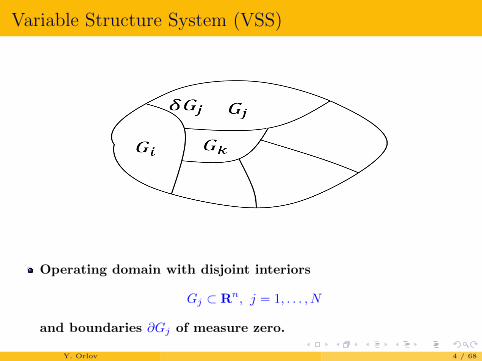
Variable Structure System (VSS)
Operating domain with disjoint interiors
Gj ⊂ Rn, j = 1, . . . , N
and boundaries ∂Gj of measure zero.
Y. Orlov 4 / 68
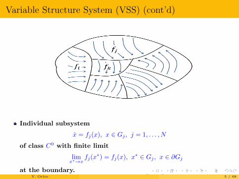
Variable Structure System (VSS) (cont’d)
Individual subsystem
x = fj(x), x ∈ Gj , j = 1, . . . , N
of class C0 with finite limit
limx∗→x
fj(x∗) = fj(x), x∗ ∈ Gj , x ∈ ∂Gj
at the boundary.In general, fj(x) 6= fi(x) for x ∈ ∂Gji = Gj ∩ Gi.Y. Orlov 5 / 68

Variable Structure DynamicsUtkin Sliding Modes in Cnntrol and Optimization Springer, 1992Edwards, Spurgeon Sliding Mode Control – Theory and Applications CRS, 1998
Significantly different from the behavior of each individualsubsystem.
Sliding Modes (SM) along the boundaries ∂Gj, if any, to bedefined
May be possible to stabilize a system by varying its structure,even if all individual subsystems are unstable.
Y. Orlov 6 / 68
Example: VSS puzzle
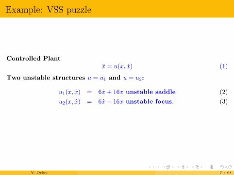
Controlled Plantx = u(x, x) (1)
Two unstable structures u = u1 and u = u2:
u1(x, x) = 6x+ 16x unstable saddle (2)
u2(x, x) = 6x− 16x unstable focus. (3)
Y. Orlov 7 / 68
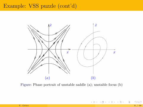
Example: VSS puzzle (cont’d)
x
x
x
x
(b)(a)
Figure: Phase portrait of unstable saddle (a); unstable focus (b)
Y. Orlov 8 / 68

Example: VSS puzzle (cont’d)
Switching rule
u(x, x) =
6x+ 16x if xs(x, x) < 06x− 16x if xs(x, x) > 0
(4)
forcing the system structure to slide along the surface
s(x, x) = x+ cx, c > 0 (5)
results in asymptotical stability of the closed-loop system.
Y. Orlov 9 / 68
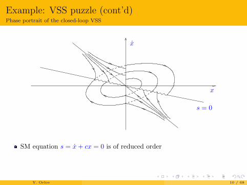
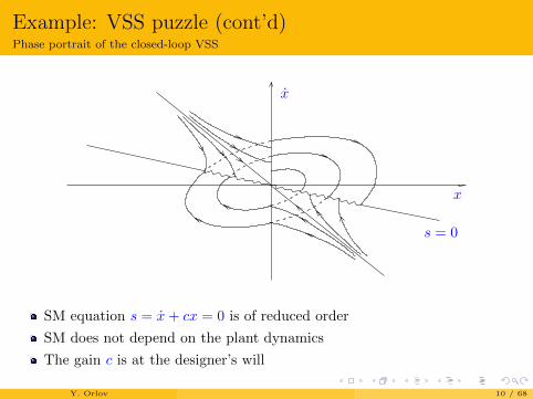
Example: VSS puzzle (cont’d)Phase portrait of the closed-loop VSS
x
x
s = 0
SM equation s = x+ cx = 0 is of reduced order
SM does not depend on the plant dynamics
The gain c is at the designer’s will
Y. Orlov 10 / 68

Example: VSS puzzle (cont’d)Phase portrait of the closed-loop VSS
x
x
s = 0
SM equation s = x+ cx = 0 is of reduced order
SM does not depend on the plant dynamics
The gain c is at the designer’s will
Y. Orlov 10 / 68
Example: VSS puzzle (cont’d)Phase portrait of the closed-loop VSS
x
x
s = 0
SM equation s = x+ cx = 0 is of reduced order
SM does not depend on the plant dynamics
The gain c is at the designer’s will
Y. Orlov 10 / 68
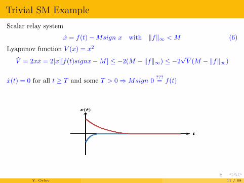
Trivial SM Example
Scalar relay system
x = f(t)−Msign x with ‖f‖∞ < M (6)
Lyapunov function V (x) = x2
V = 2xx = 2|x|[f(t)signx−M ] ≤ −2(M − ‖f‖∞) ≤ −2√V (M − ‖f‖∞)
x(t) = 0 for all t ≥ T and some T > 0⇒Msign 0???= f(t)
Y. Orlov 11 / 68
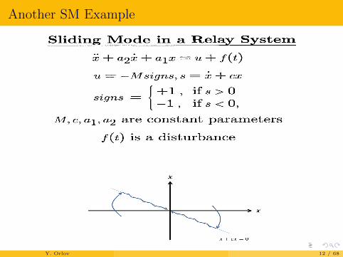
Another SM Example
Y. Orlov 12 / 68

ANTICIPATED SLIDING MODE FEATURES
Counteracting non-vanishing disturbances and plant uncertainties.
Synthesis decomposition: SM control is synthesized to steer the system toa switching manifold in finite time; after that the system slides along thismanifold selected independently of the control law.
PRINCIPAL OPERATING MODES
First order SMs occur on the manifold of co-dimension 1.Extensively developed from early 60s – Emel’yanov & Utkin school
Alternatively, the state can be forced to avoid evolving on the switchingmanifolds, while steering to their intersections of higher co-dimensionwhere HOSM (higher order sliding mode) occurs.Fuller phenomenon discovered in 1960Systematic study from late 80s – Emel’yanov, Korovin, Levantovskii
Y. Orlov 13 / 68
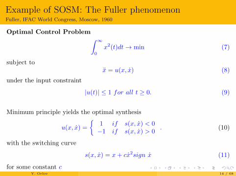
Example of SOSM: The Fuller phenomenonFuller, IFAC World Congress, Moscow, 1960
Optimal Control Problem∫ ∞0
x2(t)dt→ min (7)
subject tox = u(x, x) (8)
under the input constraint
|u(t)| ≤ 1 for all t ≥ 0. (9)
Minimum principle yields the optimal synthesis
u(x, x) =
1 if s(x, x) < 0−1 if s(x, x) > 0
. (10)
with the switching curve
s(x, x) = x+ cx2sign x (11)
for some constant cY. Orlov 14 / 68
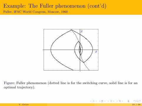
Example: The Fuller phenomenon (cont’d)Fuller, IFAC World Congress, Moscow, 1960
0
0
x
x
Figure: Fuller phenomenon (dotted line is for the switching curve, solid line is for anoptimal trajectory).
Y. Orlov 15 / 68
Example: The Fuller phenomenon featuresFuller, IFAC World Congress, Moscow, 1960
No sliding modes on the switching curve, the optimal trajectories cross itat countably many points.
The switching times have a finite accumulation point (Zeno behavior).
The closed-loop variable structure system is steered to the origin in finitetime.
After that there appears a so-called SOSM (sliding mode of the secondorder).
The sliding manifold has codimension 2, i.e., it is confined to the originonly.
Y. Orlov 16 / 68
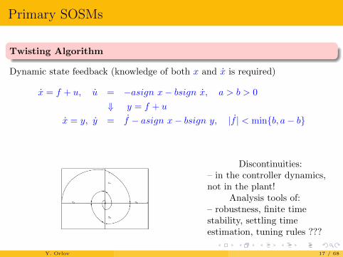
Primary SOSMs
Twisting Algorithm
Dynamic state feedback (knowledge of both x and x is required)
x = f + u, u = −asign x− bsign x, a > b > 0
⇓ y = f + u
x = y, y = f − asign x− bsign y, |f | < minb, a− b
Discontinuities:– in the controller dynamics,not in the plant!
Analysis tools of:– robustness, finite timestability, settling timeestimation, tuning rules ???
Y. Orlov 17 / 68
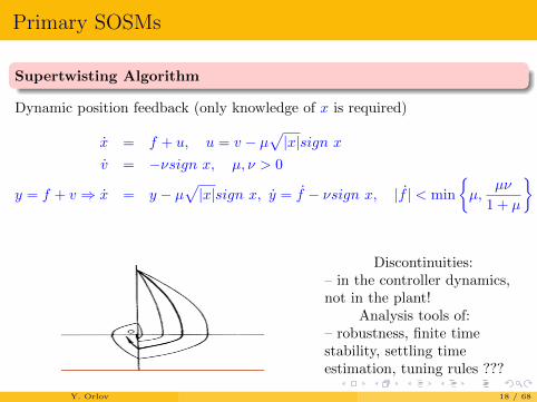
Primary SOSMs
Supertwisting Algorithm
Dynamic position feedback (only knowledge of x is required)
x = f + u, u = v − µ√|x|sign x
v = −νsign x, µ, ν > 0
y = f + v ⇒ x = y − µ√|x|sign x, y = f − νsign x, |f | < min
µ,
µν
1 + µ
Discontinuities:– in the controller dynamics,not in the plant!
Analysis tools of:– robustness, finite timestability, settling timeestimation, tuning rules ???
Y. Orlov 18 / 68

Mathematical Tools of VSS
Y. Orlov 19 / 68
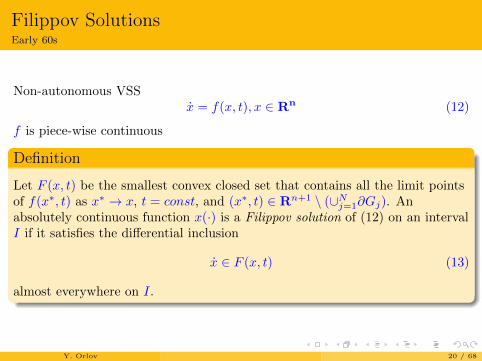
Filippov SolutionsEarly 60s
Non-autonomous VSSx = f(x, t), x ∈ Rn (12)
f is piece-wise continuous
Definition
Let F (x, t) be the smallest convex closed set that contains all the limit pointsof f(x∗, t) as x∗ → x, t = const, and (x∗, t) ∈ Rn+1 \ (∪Nj=1∂Gj). Anabsolutely continuous function x(·) is a Filippov solution of (12) on an intervalI if it satisfies the differential inclusion
x ∈ F (x, t) (13)
almost everywhere on I.
Y. Orlov 20 / 68
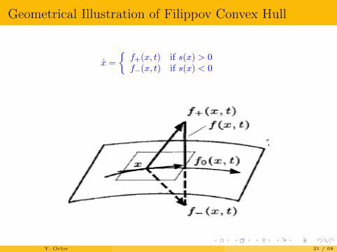
Geometrical Illustration of Filippov Convex Hull
x =
f+(x, t) if s(x) > 0f−(x, t) if s(x) < 0
Y. Orlov 21 / 68

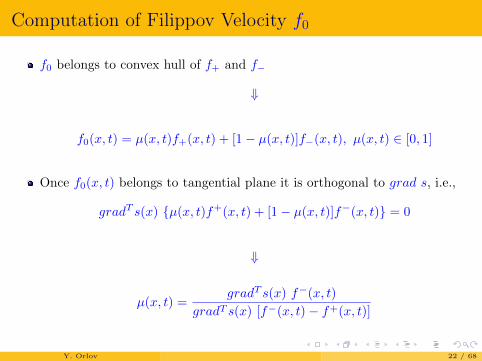
Computation of Filippov Velocity f0
f0 belongs to convex hull of f+ and f−
⇓
f0(x, t) = µ(x, t)f+(x, t) + [1− µ(x, t)]f−(x, t), µ(x, t) ∈ [0, 1]
Once f0(x, t) belongs to tangential plane it is orthogonal to grad s, i.e.,
gradT s(x) µ(x, t)f+(x, t) + [1− µ(x, t)]f−(x, t) = 0
⇓
µ(x, t) =gradT s(x) f−(x, t)
gradT s(x) [f−(x, t)− f+(x, t)]
Y. Orlov 22 / 68

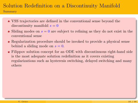
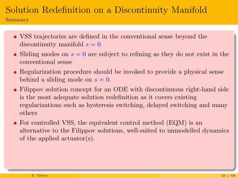
Solution Redefinition on a Discontinuity ManifoldSummary
VSS trajectories are defined in the conventional sense beyond thediscontinuity manifold s = 0
Sliding modes on s = 0 are subject to refining as they do not exist in theconventional sense
Regularization procedure should be invoked to provide a physical sensebehind a sliding mode on s = 0.
Filippov solution concept for an ODE with discontinuous right-hand sideis the most adequate solution redefinition as it covers existingregularizations such as hysteresis switching, delayed switching and manyothers
For controlled VSS, the equivalent control method (EQM) is analternative to the Filippov solutions, well-suited to unmodelled dynamicsof the applied actuator(s).
Filippov convexization and EQM result in the same provided theunderlying VSS is affine (linear in control). Just in case all possibleregularizations yield the same.
Y. Orlov 23 / 68

Stability analysis
Y. Orlov 24 / 68
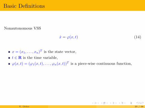
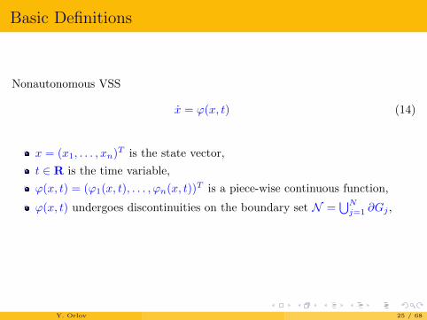
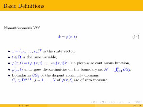
Basic Definitions
Nonautonomous VSS
x = ϕ(x, t) (14)
x = (x1, . . . , xn)T is the state vector,
t ∈ R is the time variable,
ϕ(x, t) = (ϕ1(x, t), . . . , ϕn(x, t))T is a piece-wise continuous function,
ϕ(x, t) undergoes discontinuities on the boundary set N =⋃Nj=1 ∂Gj ,
Boundaries ∂Gj of the disjoint continuity domainsGj ⊂ Rn+1, j = 1, . . . , N of ϕ(x, t) are of zero measure.
Y. Orlov 25 / 68
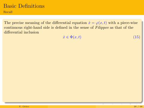
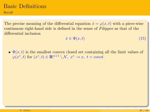
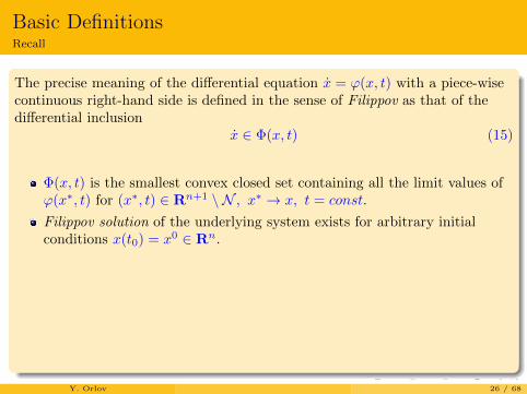
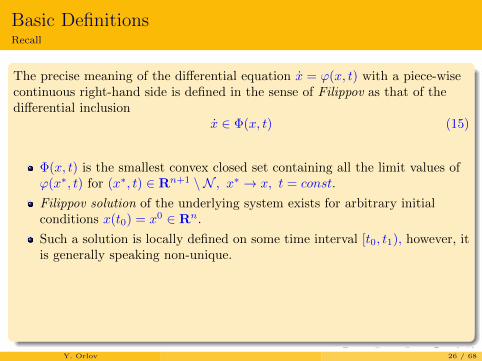
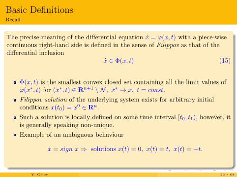
Basic DefinitionsRecall
The precise meaning of the differential equation x = ϕ(x, t) with a piece-wisecontinuous right-hand side is defined in the sense of Filippov as that of thedifferential inclusion
x ∈ Φ(x, t) (15)
Φ(x, t) is the smallest convex closed set containing all the limit values ofϕ(x∗, t) for (x∗, t) ∈ Rn+1 \ N , x∗ → x, t = const.
Filippov solution of the underlying system exists for arbitrary initialconditions x(t0) = x0 ∈ Rn.
Such a solution is locally defined on some time interval [t0, t1), however, itis generally speaking non-unique.
Example of an ambiguous behaviour
x = sign x⇒ solutions x(t) = 0, x(t) = t, x(t) = −t.
Y. Orlov 26 / 68
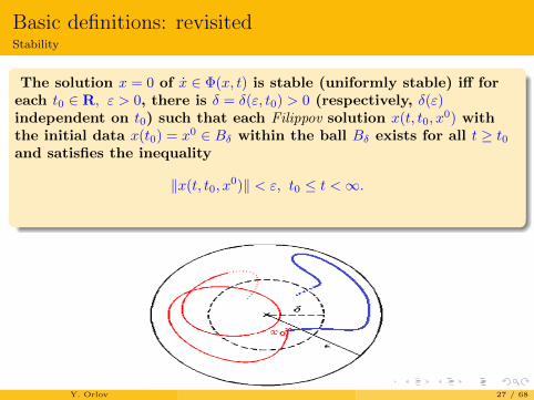
Basic definitions: revisitedStability
The solution x = 0 of x ∈ Φ(x, t) is stable (uniformly stable) iff foreach t0 ∈ R, ε > 0, there is δ = δ(ε, t0) > 0 (respectively, δ(ε)independent on t0) such that each Filippov solution x(t, t0, x
0) withthe initial data x(t0) = x0 ∈ Bδ within the ball Bδ exists for all t ≥ t0and satisfies the inequality
‖x(t, t0, x0)‖ < ε, t0 ≤ t <∞.
Y. Orlov 27 / 68
Basic definitions: revisitedAsymptotic stability
The solution x = 0 of the underlying differential inclusion is(uniformly) asymptotically stable iff it is (uniformly) stable and
limt→∞‖x(t, t0, x0)‖ = 0 (16)
holds for all solutions x(t, t0, x0) initialized within some Bδ
(uniformly in t0 and x0).
If (16) holds true for all solutions x(t, t0, x0) regardless of the
choice of the initial data (and, respectively, it is uniform in t0and x0 ∈ Bδ for each δ > 0), the solution x = 0 is said to beglobally (uniformly) asymptotically stable.
Y. Orlov 28 / 68
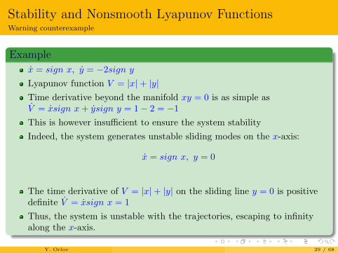
Stability and Nonsmooth Lyapunov FunctionsWarning counterexample
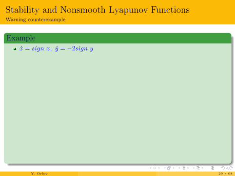
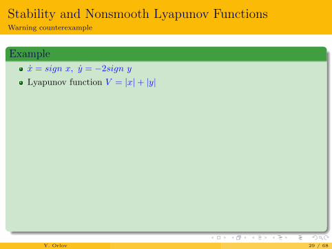
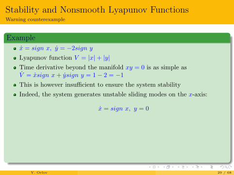
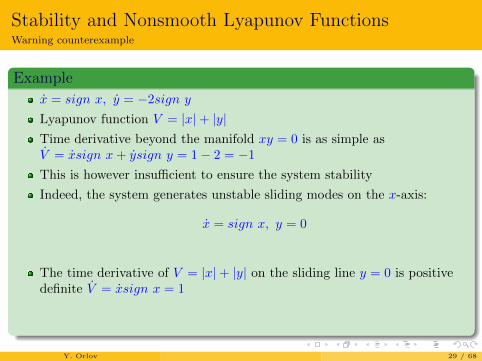
Example
x = sign x, y = −2sign y
Lyapunov function V = |x|+ |y|Time derivative beyond the manifold xy = 0 is as simple asV = xsign x+ ysign y = 1− 2 = −1
This is however insufficient to ensure the system stability
Indeed, the system generates unstable sliding modes on the x-axis:
x = sign x, y = 0
The time derivative of V = |x|+ |y| on the sliding line y = 0 is positivedefinite V = xsign x = 1
Thus, the system is unstable with the trajectories, escaping to infinityalong the x-axis.
Y. Orlov 29 / 68
Stability and Nonsmooth Lyapunov FunctionsWarning counterexample
Example
x = sign x, y = −2sign y
Lyapunov function V = |x|+ |y|
Time derivative beyond the manifold xy = 0 is as simple asV = xsign x+ ysign y = 1− 2 = −1
This is however insufficient to ensure the system stability
Indeed, the system generates unstable sliding modes on the x-axis:
x = sign x, y = 0
The time derivative of V = |x|+ |y| on the sliding line y = 0 is positivedefinite V = xsign x = 1
Thus, the system is unstable with the trajectories, escaping to infinityalong the x-axis.
Y. Orlov 29 / 68
Stability and Nonsmooth Lyapunov FunctionsWarning counterexample
Example
x = sign x, y = −2sign y
Lyapunov function V = |x|+ |y|Time derivative beyond the manifold xy = 0 is as simple asV = xsign x+ ysign y = 1− 2 = −1
This is however insufficient to ensure the system stability
Indeed, the system generates unstable sliding modes on the x-axis:
x = sign x, y = 0
The time derivative of V = |x|+ |y| on the sliding line y = 0 is positivedefinite V = xsign x = 1
Thus, the system is unstable with the trajectories, escaping to infinityalong the x-axis.
Y. Orlov 29 / 68
Stability and Nonsmooth Lyapunov FunctionsWarning counterexample
Example
x = sign x, y = −2sign y
Lyapunov function V = |x|+ |y|Time derivative beyond the manifold xy = 0 is as simple asV = xsign x+ ysign y = 1− 2 = −1
This is however insufficient to ensure the system stability
Indeed, the system generates unstable sliding modes on the x-axis:
x = sign x, y = 0
The time derivative of V = |x|+ |y| on the sliding line y = 0 is positivedefinite V = xsign x = 1
Thus, the system is unstable with the trajectories, escaping to infinityalong the x-axis.
Y. Orlov 29 / 68
Stability and Nonsmooth Lyapunov FunctionsThe analysis to be presented
Seeking for a positive (semi)definite Lipschitz-continuous Lyapunovfunction V (x, t), nonincreasing along the system trajectories.
Special attention to the behavior of the composed function V (x(t), t) onsliding manifolds and on nondifferentiability sets of V (x, t) !!!
All the system trajectories are concluded to be bounded and, due toFilippov, they prove to be globally defined, possibly non-uniquely, in thedirection of increasing t.
By applying standard Lyapunov arguments, the system stability isguaranteed.
Asymptotic stability is additionally to be studied (Barbalat lemma,extended invariance principle...)
Y. Orlov 30 / 68

Stability and Nonsmooth Lyapunov FunctionsDifferentiation Rule for a Lipschitz-continuous Function
V (x, t) is Lipschitz continuous, x(t) is a solution of x = ϕ(x, t)
⇓
The composite function V (x (t) , t) is absolutely continuous and
d
dtV (x (t) , t) =
d
dhV (x (t) + hx (t) , t+ h)
∣∣∣∣h=0
almost everywhere.
Y. Orlov 31 / 68
Lyapunov approachExtension to VSS
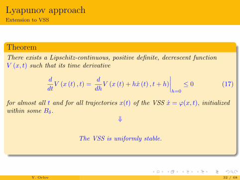
TheoremThere exists a Lipschitz-continuous, positive definite, decrescent functionV (x, t) such that its time derivative
d
dtV (x (t) , t) =
d
dhV (x (t) + hx (t) , t+ h)
∣∣∣∣h=0
≤ 0 (17)
for almost all t and for all trajectories x(t) of the VSS x = ϕ(x, t), initializedwithin some Bδ.
⇓
The VSS is uniformly stable.
Y. Orlov 32 / 68
Taking care just at the nondifferentiability set of V
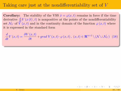
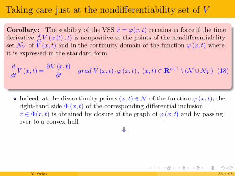
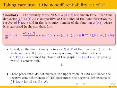
Corollary: The stability of the VSS x = ϕ(x, t) remains in force if the timederivative d
dtV (x (t) , t) is nonpositive at the points of the nondifferentiabilityset NV of V (x, t) and in the continuity domain of the function ϕ (x, t) whereit is expressed in the standard form
d
dtV (x, t) =
∂V (x, t)
∂t+ grad V (x, t) ·ϕ (x, t) , (x, t) ∈ Rn+1 \ (N ∪NV ) (18)
Indeed, at the discontinuity points (x, t) ∈ N of the function ϕ (x, t), theright-hand side Φ (x, t) of the corresponding differential inclusionx ∈ Φ(x, t) is obtained by closure of the graph of ϕ (x, t) and by passingover to a convex hull.
⇓
These procedures do not increase the upper value of (18) and hence thenegative semidefiniteness of (18) guarantees the negative definiteness ofddtV (x, t) for all (x, t) ∈ N .
Y. Orlov 33 / 68
Taking care just at the nondifferentiability set of V
Corollary: The stability of the VSS x = ϕ(x, t) remains in force if the timederivative d
dtV (x (t) , t) is nonpositive at the points of the nondifferentiabilityset NV of V (x, t) and in the continuity domain of the function ϕ (x, t) whereit is expressed in the standard form
d
dtV (x, t) =
∂V (x, t)
∂t+ grad V (x, t) ·ϕ (x, t) , (x, t) ∈ Rn+1 \ (N ∪NV ) (18)
Indeed, at the discontinuity points (x, t) ∈ N of the function ϕ (x, t), theright-hand side Φ (x, t) of the corresponding differential inclusionx ∈ Φ(x, t) is obtained by closure of the graph of ϕ (x, t) and by passingover to a convex hull.
⇓
These procedures do not increase the upper value of (18) and hence thenegative semidefiniteness of (18) guarantees the negative definiteness ofddtV (x, t) for all (x, t) ∈ N .
Y. Orlov 33 / 68
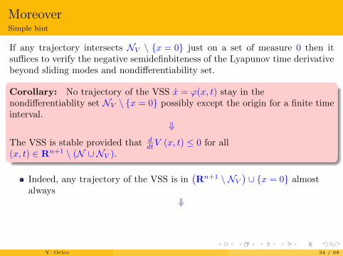
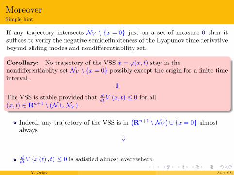
MoreoverSimple hint
If any trajectory intersects NV \ x = 0 just on a set of measure 0 then itsuffices to verify the negative semidefinbiteness of the Lyapunov time derivativebeyond sliding modes and nondifferentiability set.
Corollary: No trajectory of the VSS x = ϕ(x, t) stay in thenondifferentiablity set NV \ x = 0 possibly except the origin for a finite timeinterval.
⇓
The VSS is stable provided that ddtV (x, t) ≤ 0 for all
(x, t) ∈ Rn+1 \ (N ∪NV ).
Indeed, any trajectory of the VSS is in(Rn+1 \ NV
)∪ x = 0 almost
always⇓
ddtV (x (t) , t) ≤ 0 is satisfied almost everywhere.
Y. Orlov 34 / 68

Krasovskii–LaSalle Invariance Principle
Ensures the convergence of the state trajectories x (t) to the largestinvariant subset M of the manifold where the time derivative of theLyapunov function takes no value.
M ⊂ Rn is an invariant set of (14) if, for all x0 ∈M , the trajectoriesinitialized at x0 at some time t0 remain in M for all t > t0.
Proven for autonomous continuous dynamic systems
In general, not valid for non-autonomous systems
Non-extendible to general differential inclusions and, particularly, todiscontinuous dynamic systems, possibly, due to their ambiguousbehavior.
Y. Orlov 35 / 68
Invariance PrincipleExtension to a Class of Discontinuous Systems
The invariance principle remains in force for autonomous VSS
x = ϕ (x) ,
whose solutions are uniquely continuable to the right.
Sufficient right uniqueness conditions for solutions of the above system andcontinuous dependence of the solutions on their initial data have been carriedout by Filippov.
Y. Orlov 36 / 68
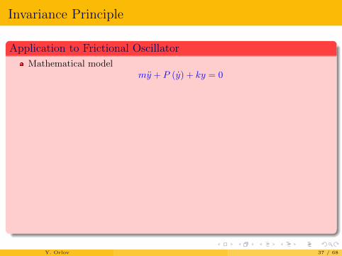
Invariance Principle
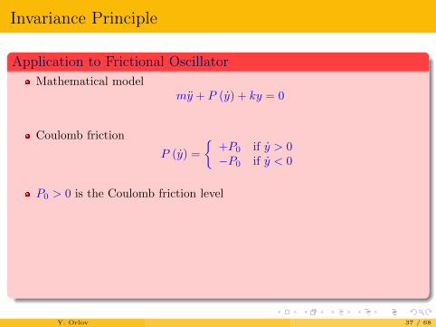
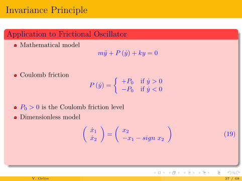
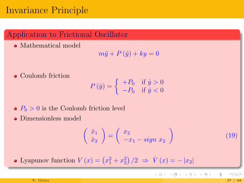
Application to Frictional Oscillator
Mathematical modelmy + P (y) + ky = 0
Coulomb friction
P (y) =
+P0 if y > 0−P0 if y < 0
P0 > 0 is the Coulomb friction level
Dimensionless model (x1
x2
)=
(x2
−x1 − sign x2
)(19)
Lyapunov function V (x) =(x2
1 + x22
)/2 ⇒ V (x) = − |x2|
Y. Orlov 37 / 68

Invariance Principle
Application to Frictional Oscillator
Mathematical modelmy + P (y) + ky = 0
Coulomb friction
P (y) =
+P0 if y > 0−P0 if y < 0
P0 > 0 is the Coulomb friction level
Dimensionless model (x1
x2
)=
(x2
−x1 − sign x2
)(19)
Lyapunov function V (x) =(x2
1 + x22
)/2 ⇒ V (x) = − |x2|
Y. Orlov 37 / 68

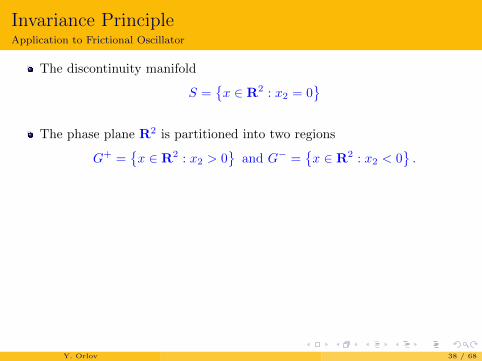
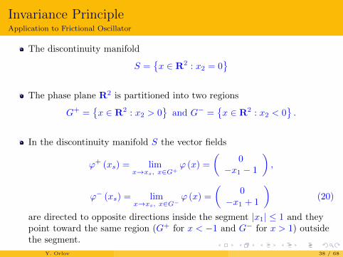
Invariance PrincipleApplication to Frictional Oscillator
The discontinuity manifold
S =x ∈ R2 : x2 = 0
The phase plane R2 is partitioned into two regions
G+ =x ∈ R2 : x2 > 0
and G− =
x ∈ R2 : x2 < 0
.
In the discontinuity manifold S the vector fields
ϕ+ (xs) = limx→xs, x∈G+
ϕ (x) =
(0
−x1 − 1
),
ϕ− (xs) = limx→xs, x∈G−
ϕ (x) =
(0
−x1 + 1
)(20)
are directed to opposite directions inside the segment |x1| ≤ 1 and theypoint toward the same region (G+ for x < −1 and G− for x > 1) outsidethe segment.
Y. Orlov 38 / 68
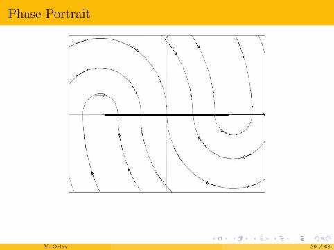
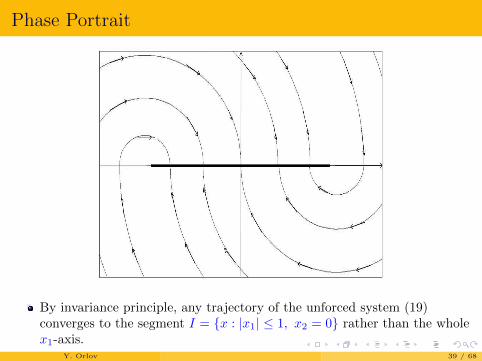
Phase Portrait
By invariance principle, any trajectory of the unforced system (19)converges to the segment I = x : |x1| ≤ 1, x2 = 0 rather than the wholex1-axis.
Y. Orlov 39 / 68
Phase Portrait
By invariance principle, any trajectory of the unforced system (19)converges to the segment I = x : |x1| ≤ 1, x2 = 0 rather than the wholex1-axis.
Y. Orlov 39 / 68
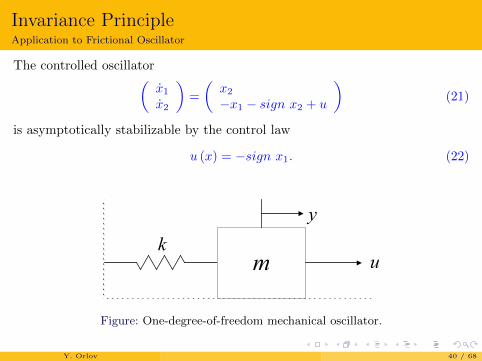
Invariance PrincipleApplication to Frictional Oscillator
The controlled oscillator(x1
x2
)=
(x2
−x1 − sign x2 + u
)(21)
is asymptotically stabilizable by the control law
u (x) = −sign x1. (22)
y
m uk
Figure: One-degree-of-freedom mechanical oscillator.
Y. Orlov 40 / 68
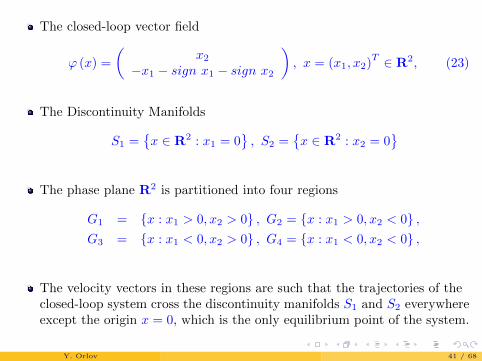
The closed-loop vector field
ϕ (x) =
(x2
−x1 − sign x1 − sign x2
), x = (x1, x2)
T ∈ R2, (23)
The Discontinuity Manifolds
S1 =x ∈ R2 : x1 = 0
, S2 =
x ∈ R2 : x2 = 0
The phase plane R2 is partitioned into four regions
G1 = x : x1 > 0, x2 > 0 , G2 = x : x1 > 0, x2 < 0 ,G3 = x : x1 < 0, x2 > 0 , G4 = x : x1 < 0, x2 < 0 ,
The velocity vectors in these regions are such that the trajectories of theclosed-loop system cross the discontinuity manifolds S1 and S2 everywhereexcept the origin x = 0, which is the only equilibrium point of the system.
Y. Orlov 41 / 68
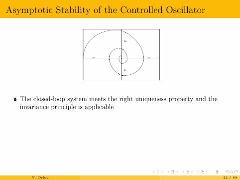
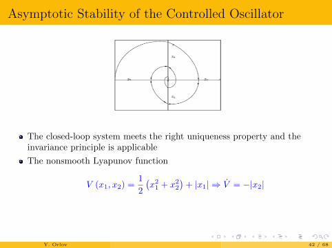
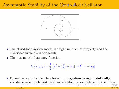
Asymptotic Stability of the Controlled Oscillator
The closed-loop system meets the right uniqueness property and theinvariance principle is applicable
The nonsmooth Lyapunov function
V (x1, x2) =1
2
(x2
1 + x22
)+ |x1| ⇒ V = −|x2|
By invariance principle, the closed loop system is asymptoticallystable because the largest invariant manifold is now reduced to the origin.
Y. Orlov 42 / 68
Finite-time Stability of Uncertain Homogeneous andQuasihomogeneous Systems
Y. Orlov 43 / 68

Uncertain Systems and Equiuniform (Robust) Stability
Perturbed VSS’
x = ϕ(x, t) + ψ(x, t), x ∈ Rn (24)
Disturbance ψ(x, t) = (ψ1(x, t), . . . , ψn(x, t))T is piece-wise continuous
Uniform Boundedness of Admissible Disturbances
|ψi(x, t)| ≤Mi, i = 1, . . . , n (25)
for almost all (x, t) ∈ Bδ ×R and some constants Mi ≥ 0, fixed a priori.
The above equation (24) is viewed as an uncertain differential equationwith rectangular uncertainties, whose Filippov solutions xψ are associatedwith an admissible disturbance ψ
Y. Orlov 44 / 68
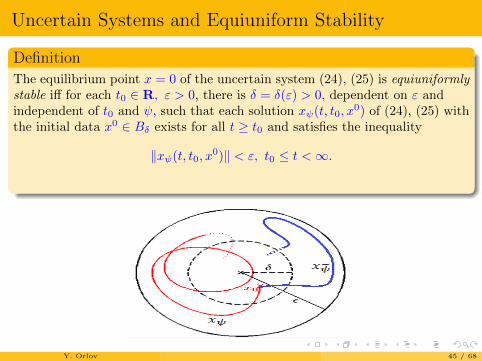
Uncertain Systems and Equiuniform Stability
Definition
The equilibrium point x = 0 of the uncertain system (24), (25) is equiuniformlystable iff for each t0 ∈ R, ε > 0, there is δ = δ(ε) > 0, dependent on ε andindependent of t0 and ψ, such that each solution xψ(t, t0, x
0) of (24), (25) withthe initial data x0 ∈ Bδ exists for all t ≥ t0 and satisfies the inequality
‖xψ(t, t0, x0)‖ < ε, t0 ≤ t <∞.
Y. Orlov 45 / 68
Uncertain Systems and Equiuniform Stability
Definition
The equilibrium point x = 0 of the uncertain system (24), (25) is said to beequiuniformly asymptotically stable if it is equiuniformly stable and theconvergence
limt→∞‖xψ(t, t0, x0)‖ = 0 (26)
holds for all solutions of (24), (25) initialized within some Bδ, uniformly in theinitial data t0 and x0, and all the solutions xψ(·, t0, x0). If this convergenceremains in force for each δ > 0 the equilibrium point is said to be globallyequiuniformly asymptotically stable.
Y. Orlov 46 / 68
Uncertain Systems and Equiuniform Stability
Definition
The equilibrium point x = 0 of the uncertain system (24), (25) is said to beglobally equiuniformly finite-time stable if, in addition to the globalequiuniform asymptotical stability, the limiting relation
xψ(t, t0, x0) = 0 (27)
holds for each solution xψ(·, t0, x0) and all t ≥ t0 + T (t0, x0) where the settling
time function
T (t0, x0) = sup
xψ(·,t0,x0)
infT ≥ 0 : xψ(t, t0, x0) = 0 for all t ≥ t0 + T (28)
is such that
T (Bδ) = supt0∈R, x0∈BδT (t0, x0) <∞ for each δ > 0.
.
Y. Orlov 47 / 68
Homogeneous Functions
Definition
A piece-wise continuous function ϕ(x, t) is called locally homogeneous of degreeq ∈ R with respect to dilation (r1, . . . , rn) where ri > 0, i = 1, . . . , n if thereexist a constant c0 > 0 and a ball Bδ ⊂ Rn such that
ϕi(cr1x1, . . . , c
rnxn, c−qt) = cq+riϕi(x1, . . . , xn, t) (29)
for all c ≥ c0 and almost all (x, t) ∈ Bδ ×R.
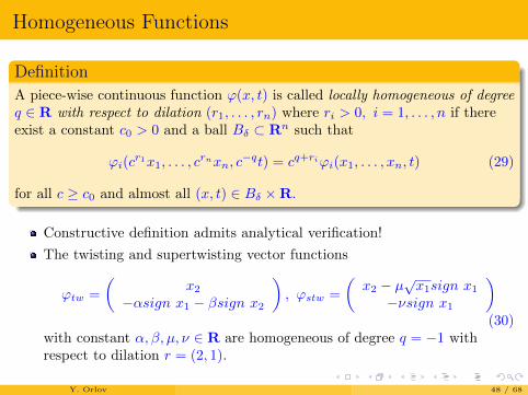
Constructive definition admits analytical verification!
The twisting and supertwisting vector functions
ϕtw =
(x2
−αsign x1 − βsign x2
), ϕstw =
(x2 − µ
√x1sign x1
−νsign x1
)(30)
with constant α, β, µ, ν ∈ R are homogeneous of degree q = −1 withrespect to dilation r = (2, 1).
Y. Orlov 48 / 68

Homogeneous Functions
Definition
A piece-wise continuous function ϕ(x, t) is called locally homogeneous of degreeq ∈ R with respect to dilation (r1, . . . , rn) where ri > 0, i = 1, . . . , n if thereexist a constant c0 > 0 and a ball Bδ ⊂ Rn such that
ϕi(cr1x1, . . . , c
rnxn, c−qt) = cq+riϕi(x1, . . . , xn, t) (29)
for all c ≥ c0 and almost all (x, t) ∈ Bδ ×R.
Constructive definition admits analytical verification!
The twisting and supertwisting vector functions
ϕtw =
(x2
−αsign x1 − βsign x2
), ϕstw =
(x2 − µ
√x1sign x1
−νsign x1
)(30)
with constant α, β, µ, ν ∈ R are homogeneous of degree q = −1 withrespect to dilation r = (2, 1).
Y. Orlov 48 / 68
Quasihomogeneous Uncertain Systems
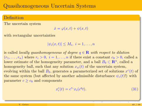
DefinitionThe uncertain system
x = ϕ(x, t) + ψ(x, t)
with rectangular uncertainties
|ψi(x, t)| ≤Mi, i = 1, . . . , n
is called locally quasihomogeneous of degree q ∈ R with respect to dilation(r1, . . . , rn) where ri > 0, i = 1, . . . , n if there exist a constant c0 > 0, called alower estimate of the homogeneity parameter, and a ball Bδ ⊂ Rn, called ahomogeneity ball, such that any solution xψ(t) of the uncertain system,evolving within the ball Bδ, generates a parameterized set of solutions xc(t) ofthe same system (but affected by another admissible disturbance ψc(t)!) withparameter c ≥ c0 and components
xci (t) = crixi(cqt). (31)
Y. Orlov 49 / 68
Homogeneous Functions Generate QuasihomogeneousUncertain Systems
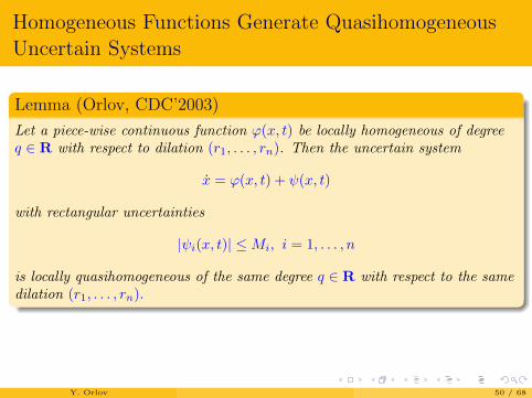
Lemma (Orlov, CDC’2003)
Let a piece-wise continuous function ϕ(x, t) be locally homogeneous of degreeq ∈ R with respect to dilation (r1, . . . , rn). Then the uncertain system
x = ϕ(x, t) + ψ(x, t)
with rectangular uncertainties
|ψi(x, t)| ≤Mi, i = 1, . . . , n
is locally quasihomogeneous of the same degree q ∈ R with respect to the samedilation (r1, . . . , rn).
Proof is based on embedding a quasihomogeneous uncertain system intoan appropriate framework of homogeneous differential inclusion.
Y. Orlov 50 / 68

Homogeneous Functions Generate QuasihomogeneousUncertain Systems
Lemma (Orlov, CDC’2003)
Let a piece-wise continuous function ϕ(x, t) be locally homogeneous of degreeq ∈ R with respect to dilation (r1, . . . , rn). Then the uncertain system
x = ϕ(x, t) + ψ(x, t)
with rectangular uncertainties
|ψi(x, t)| ≤Mi, i = 1, . . . , n
is locally quasihomogeneous of the same degree q ∈ R with respect to the samedilation (r1, . . . , rn).
Proof is based on embedding a quasihomogeneous uncertain system intoan appropriate framework of homogeneous differential inclusion.
Y. Orlov 50 / 68
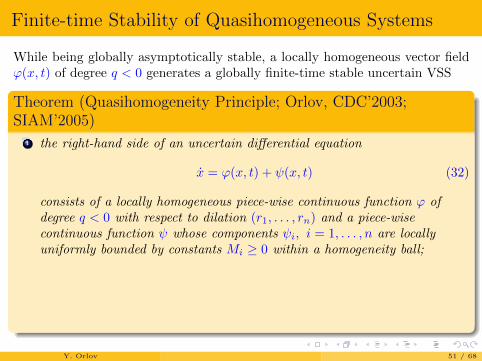
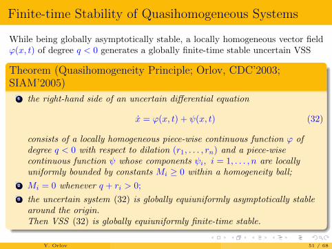
Finite-time Stability of Quasihomogeneous Systems
While being globally asymptotically stable, a locally homogeneous vector fieldϕ(x, t) of degree q < 0 generates a globally finite-time stable uncertain VSS
Theorem (Quasihomogeneity Principle; Orlov, CDC’2003;SIAM’2005)
1 the right-hand side of an uncertain differential equation
x = ϕ(x, t) + ψ(x, t) (32)
consists of a locally homogeneous piece-wise continuous function ϕ ofdegree q < 0 with respect to dilation (r1, . . . , rn) and a piece-wisecontinuous function ψ whose components ψi, i = 1, . . . , n are locallyuniformly bounded by constants Mi ≥ 0 within a homogeneity ball;
2 Mi = 0 whenever q + ri > 0;
3 the uncertain system (32) is globally equiuniformly asymptotically stablearound the origin.Then VSS (32) is globally equiuniformly finite-time stable.
Y. Orlov 51 / 68

Settling Time EstimateOrlov, SICON 2005
Going through this route yields:Upper Estimate
T (t0, x0) ≤ τ(x0, ER) +
1
1− 2q(δR−1)qs(δ)
of the settling-time function
T (t0, x0) = sup
x(·,t0,x0)
infT ≥ 0 : x(t, t0, x0) = 0 for all t ≥ t0 + T
in terms of the reaching-time function
τ(x0, ER) = supx(·,t0,x0)
infT ≥ 0 : x(t, t0, x0) ∈ ER for all t0 ∈ R, t ≥ t0 + T
of attaining the ellipsoid
ER = x ∈ Rn :
√Σni=1
( xiRri
)2
≤ 1,
and the semidistance-time function
s(δ) = supx0∈Eδ
τ(x0, E 12 δ
)Y. Orlov 52 / 68
Arsenal of Finite-time Stability Analysis Tools
Y. Orlov 53 / 68
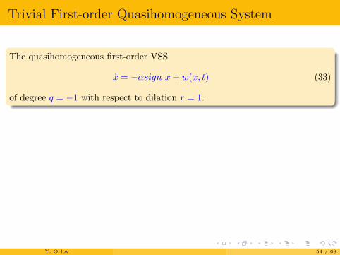
Trivial First-order Quasihomogeneous System
The quasihomogeneous first-order VSS
x = −αsign x+ w(x, t) (33)
of degree q = −1 with respect to dilation r = 1.
Uniform Upper Bound on Disturbance magnitude
|w(x, t)| ≤ N
The higher switching magnitude is chosen:
α > N > 0
Y. Orlov 54 / 68
Trivial First-order Quasihomogeneous System
The quasihomogeneous first-order VSS
x = −αsign x+ w(x, t) (33)
of degree q = −1 with respect to dilation r = 1.
Uniform Upper Bound on Disturbance magnitude
|w(x, t)| ≤ N
The higher switching magnitude is chosen:
α > N > 0
Y. Orlov 54 / 68
Trivial First-order Quasihomogeneous System
The quasihomogeneous first-order VSS
x = −αsign x+ w(x, t) (33)
of degree q = −1 with respect to dilation r = 1.
Uniform Upper Bound on Disturbance magnitude
|w(x, t)| ≤ N
The higher switching magnitude is chosen:
α > N > 0
Y. Orlov 54 / 68
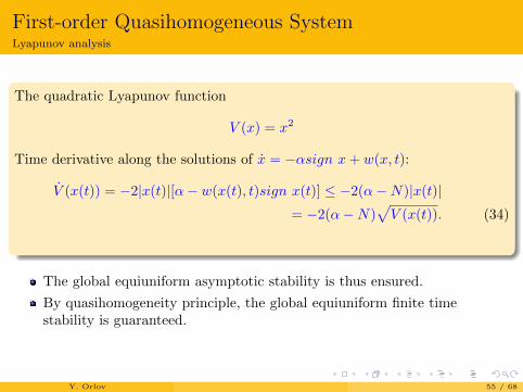
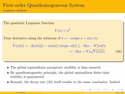
First-order Quasihomogeneous SystemLyapunov analysis
The quadratic Lyapunov function
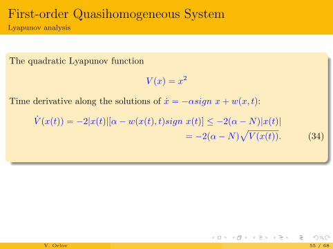
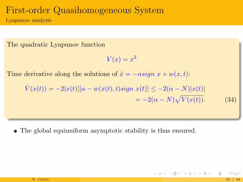
V (x) = x2
Time derivative along the solutions of x = −αsign x+ w(x, t):
V (x(t)) = −2|x(t)|[α− w(x(t), t)sign x(t)] ≤ −2(α−N)|x(t)|= −2(α−N)
√V (x(t)). (34)
The global equiuniform asymptotic stability is thus ensured.
By quasihomogeneity principle, the global equiuniform finite timestability is guaranteed.
Remark, the decay rate (34) itself results in the same conclusion. Indeed
Y. Orlov 55 / 68
First-order Quasihomogeneous SystemLyapunov analysis
The quadratic Lyapunov function
V (x) = x2
Time derivative along the solutions of x = −αsign x+ w(x, t):
V (x(t)) = −2|x(t)|[α− w(x(t), t)sign x(t)] ≤ −2(α−N)|x(t)|= −2(α−N)
√V (x(t)). (34)
The global equiuniform asymptotic stability is thus ensured.
By quasihomogeneity principle, the global equiuniform finite timestability is guaranteed.
Remark, the decay rate (34) itself results in the same conclusion. Indeed
Y. Orlov 55 / 68
Finite-time Stability of Useful Differential Inequality
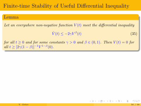
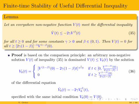
Lemma
Let an everywhere non-negative function V (t) meet the differential inequality
V (t) ≤ −2γV β(t) (35)
for all t ≥ 0 and for some constants γ > 0 and β ∈ (0, 1). Then V (t) = 0 forall t ≥ [2γ(1− β)]−1V 1−β(0).
Proof is based on the comparison principle: an arbitrary non-negativesolution V (t) of inequality (35) is dominated V (t) ≤ V0(t) by the solution
V0(t) =
[V (1−β)(0)− 2γ(1− β)t]1
1−β if t ∈ [0, V(1−β)(0)
2γ(1−β) ]
0 if t ≥ V (1−β)(0)2γ(1−β)
(36)
of the differential equation
V0(t) = −2γV β0 (t),
specified with the same initial condition V0(0) = V (0).
Y. Orlov 56 / 68
Finite-time Stability of Useful Differential Inequality
Lemma
Let an everywhere non-negative function V (t) meet the differential inequality
V (t) ≤ −2γV β(t) (35)
for all t ≥ 0 and for some constants γ > 0 and β ∈ (0, 1). Then V (t) = 0 forall t ≥ [2γ(1− β)]−1V 1−β(0).
Proof is based on the comparison principle: an arbitrary non-negativesolution V (t) of inequality (35) is dominated V (t) ≤ V0(t) by the solution
V0(t) =
[V (1−β)(0)− 2γ(1− β)t]1
1−β if t ∈ [0, V(1−β)(0)
2γ(1−β) ]
0 if t ≥ V (1−β)(0)2γ(1−β)
(36)
of the differential equation
V0(t) = −2γV β0 (t),
specified with the same initial condition V0(0) = V (0).
Y. Orlov 56 / 68
Finite-time Stability of Supertwisting AlgorithmOrlov, Aoustin, Chevallereau, IEEE TAC 2011
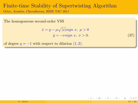
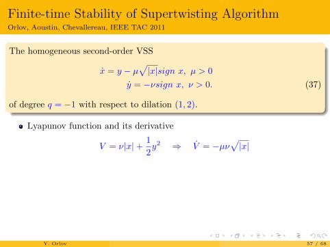
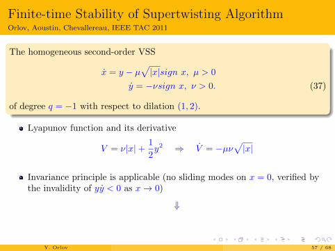
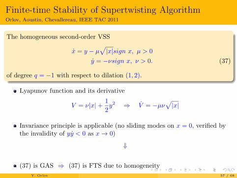
The homogeneous second-order VSS
x = y − µ√|x|sign x, µ > 0
y = −νsign x, ν > 0. (37)
of degree q = −1 with respect to dilation (1, 2).
Lyapunov function and its derivative
V = ν|x|+ 1
2y2 ⇒ V = −µν
√|x|
Invariance principle is applicable (no sliding modes on x = 0, verified bythe invalidity of yy < 0 as x→ 0)
⇓
(37) is GAS ⇒ (37) is FTS due to homogeneity
Y. Orlov 57 / 68
Finite-time Stability of Supertwisting AlgorithmOrlov, Aoustin, Chevallereau, IEEE TAC 2011
The homogeneous second-order VSS
x = y − µ√|x|sign x, µ > 0
y = −νsign x, ν > 0. (37)
of degree q = −1 with respect to dilation (1, 2).
Lyapunov function and its derivative
V = ν|x|+ 1
2y2 ⇒ V = −µν
√|x|
Invariance principle is applicable (no sliding modes on x = 0, verified bythe invalidity of yy < 0 as x→ 0)
⇓
(37) is GAS ⇒ (37) is FTS due to homogeneity
Y. Orlov 57 / 68
Robust Finite-time Stability of Supertwisting AlgorithmMoreno, Osorio, CDC’2008 & Orlov, Aoustin, Chevallereau , IEEE TAC 2011
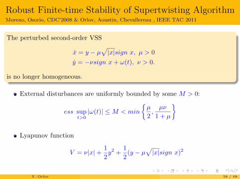
The perturbed second-order VSS
x = y − µ√|x|sign x, µ > 0
y = −νsign x+ ω(t), ν > 0.
is no longer homogeneous.
External disturbances are uniformly bounded by some M > 0:
ess supt>0|ω(t)| ≤M < min
µ
2,µν
1 + µ
Lyapunov function
V = ν|x|+ 1
2y2 +
1
2(y − µ
√|x|sign x)2
Y. Orlov 58 / 68

Robust Finite-time Stability of Supertwisting AlgorithmMoreno, Osorio, CDC’2008 & Orlov, Aoustin, Chevallereau , IEEE TAC 2011
The perturbed second-order VSS
x = y − µ√|x|sign x, µ > 0
y = −νsign x+ ω(t), ν > 0.
is no longer homogeneous.
External disturbances are uniformly bounded by some M > 0:
ess supt>0|ω(t)| ≤M < min
µ
2,µν
1 + µ
Lyapunov function
V = ν|x|+ 1
2y2 +
1
2(y − µ
√|x|sign x)2
Y. Orlov 58 / 68
Robust Finite-time Stability of Supertwisting AlgorithmOrlov, Aoustin, Chevallereau, IEEE TAC 2011
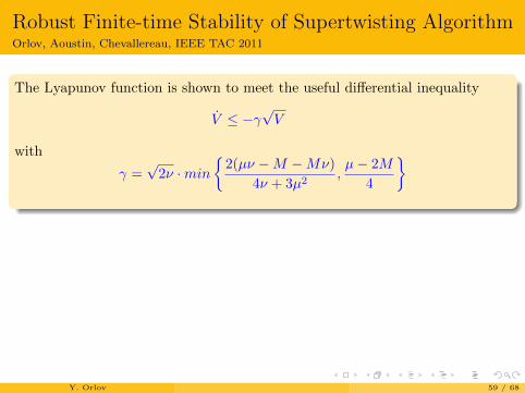
The Lyapunov function is shown to meet the useful differential inequality
V ≤ −γ√V
with
γ =√
2ν ·min
2(µν −M −Mν)
4ν + 3µ2,µ− 2M
4
⇓
Robust (equiuniform) finite time stability is thus guaranteed with thesettling time estimate
T (x0, y0) ≤ 2√V (x0, y0)γ−1
Y. Orlov 59 / 68

Robust Finite-time Stability of Supertwisting AlgorithmOrlov, Aoustin, Chevallereau, IEEE TAC 2011
The Lyapunov function is shown to meet the useful differential inequality
V ≤ −γ√V
with
γ =√
2ν ·min
2(µν −M −Mν)
4ν + 3µ2,µ− 2M
4
⇓
Robust (equiuniform) finite time stability is thus guaranteed with thesettling time estimate
T (x0, y0) ≤ 2√V (x0, y0)γ−1
Y. Orlov 59 / 68
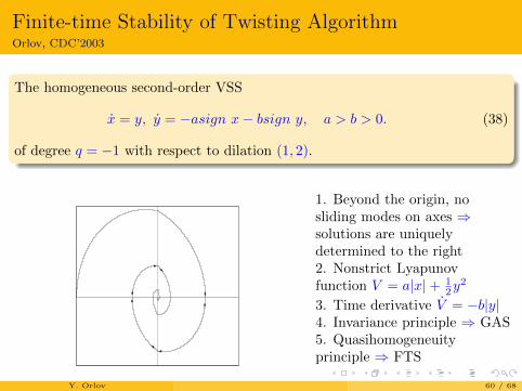
Finite-time Stability of Twisting AlgorithmOrlov, CDC’2003
The homogeneous second-order VSS
x = y, y = −asign x− bsign y, a > b > 0. (38)
of degree q = −1 with respect to dilation (1, 2).
1. Beyond the origin, nosliding modes on axes ⇒solutions are uniquelydetermined to the right2. Nonstrict Lyapunovfunction V = a|x|+ 1
2y2
3. Time derivative V = −b|y|4. Invariance principle ⇒ GAS5. Quasihomogeneuityprinciple ⇒ FTS
Y. Orlov 60 / 68
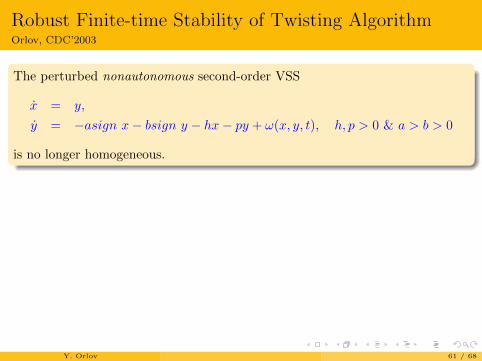
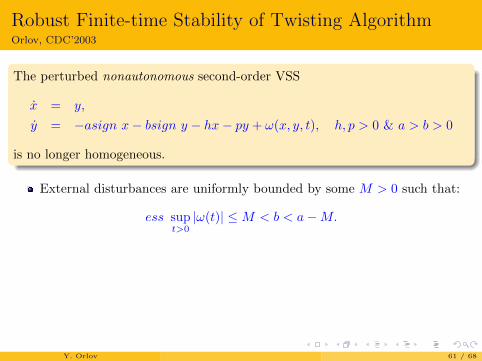
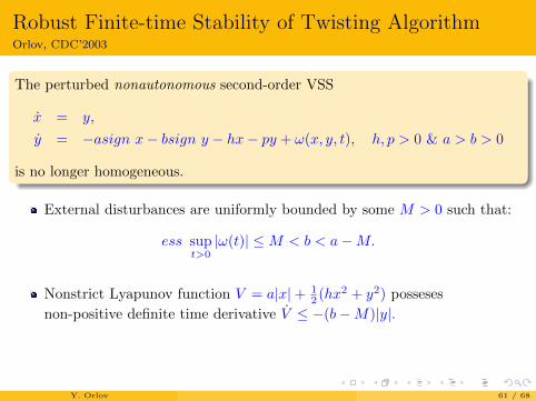
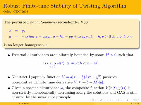
Robust Finite-time Stability of Twisting AlgorithmOrlov, CDC’2003
The perturbed nonautonomous second-order VSS
x = y,
y = −asign x− bsign y − hx− py + ω(x, y, t), h, p > 0 & a > b > 0
is no longer homogeneous.
External disturbances are uniformly bounded by some M > 0 such that:
ess supt>0|ω(t)| ≤M < b < a−M.
Nonstrict Lyapunov function V = a|x|+ 12 (hx2 + y2) posseses
non-positive definite time derivative V ≤ −(b−M)|y|.Given a specific disturbance ω, the composite function V (x(t), y(t)) isnon-strictly monotonically decreasing along the solutions and GAS is stillensured by the invariance principle.
Y. Orlov 61 / 68
Robust Finite-time Stability of Twisting AlgorithmOrlov, CDC’2003
The perturbed nonautonomous second-order VSS
x = y,
y = −asign x− bsign y − hx− py + ω(x, y, t), h, p > 0 & a > b > 0
is no longer homogeneous.
External disturbances are uniformly bounded by some M > 0 such that:
ess supt>0|ω(t)| ≤M < b < a−M.
Nonstrict Lyapunov function V = a|x|+ 12 (hx2 + y2) posseses
non-positive definite time derivative V ≤ −(b−M)|y|.
Given a specific disturbance ω, the composite function V (x(t), y(t)) isnon-strictly monotonically decreasing along the solutions and GAS is stillensured by the invariance principle.
Y. Orlov 61 / 68
Robust Finite-time Stability of Twisting AlgorithmOrlov, CDC’2003
The perturbed nonautonomous second-order VSS
x = y,
y = −asign x− bsign y − hx− py + ω(x, y, t), h, p > 0 & a > b > 0
is no longer homogeneous.
External disturbances are uniformly bounded by some M > 0 such that:
ess supt>0|ω(t)| ≤M < b < a−M.
Nonstrict Lyapunov function V = a|x|+ 12 (hx2 + y2) posseses
non-positive definite time derivative V ≤ −(b−M)|y|.Given a specific disturbance ω, the composite function V (x(t), y(t)) isnon-strictly monotonically decreasing along the solutions and GAS is stillensured by the invariance principle.
Y. Orlov 61 / 68
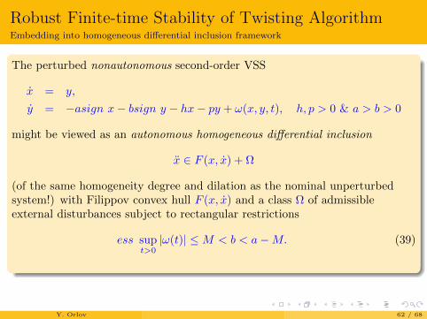
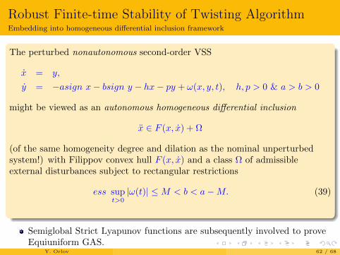
Robust Finite-time Stability of Twisting AlgorithmEmbedding into homogeneous differential inclusion framework
The perturbed nonautonomous second-order VSS
x = y,
y = −asign x− bsign y − hx− py + ω(x, y, t), h, p > 0 & a > b > 0
might be viewed as an autonomous homogeneous differential inclusion
x ∈ F (x, x) + Ω
(of the same homogeneity degree and dilation as the nominal unperturbedsystem!) with Filippov convex hull F (x, x) and a class Ω of admissibleexternal disturbances subject to rectangular restrictions
ess supt>0|ω(t)| ≤M < b < a−M. (39)
Semiglobal Strict Lyapunov functions are subsequently involved to proveEquiuniform GAS.
Y. Orlov 62 / 68
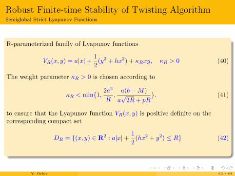
Robust Finite-time Stability of Twisting AlgorithmSemiglobal Strict Lyapunov Functions
R-parameterized family of Lyapunov functions
VR(x, y) = a|x|+ 1
2(y2 + hx2) + κRxy, κR > 0 (40)
The weight parameter κR > 0 is chosen according to
κR < min1, 2a2
R,a(b−M)
a√
2R+ pR. (41)
to ensure that the Lyapunov function VR(x, y) is positive definite on thecorresponding compact set
DR = (x, y) ∈ R2 : a|x|+ 1
2(hx2 + y2) ≤ R (42)
Y. Orlov 63 / 68
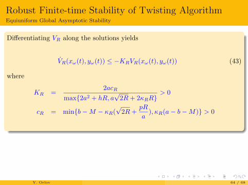
Robust Finite-time Stability of Twisting AlgorithmEquiuniform Global Asymptotic Stability
Differentiating VR along the solutions yields
VR(xω(t), yω(t)) ≤ −KRVR(xω(t), yω(t)) (43)
where
KR =2acR
max2a2 + hR, a√
2R+ 2κRR> 0
cR = minb−M − κR(√
2R+pR
a), κR(a− b−M) > 0
Semiglobal (not global!) equiuniform exponentail stability is established:
VR(xω(t), yω(t)) ≤ VR(xω(t0), yω(t0))e−KR(t−t0)
and Equiuniform GAS follows
Y. Orlov 64 / 68
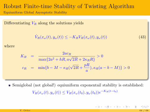
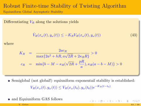
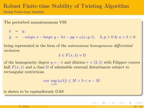
Robust Finite-time Stability of Twisting AlgorithmGlobal Finite-time Stability
The perturbed nonautonomous VSS
x = y,
y = −asign x− bsign y − hx− py + ω(x, y, t), h, p > 0 & a > b > 0
being represented in the form of the autonomous homogeneous differentialinclusion
x ∈ F (x, x) + Ω
of the homogeneity degree q = −1 and dilation r = (2, 1) with Filippov convexhull F (x, x) and a class Ω of admissible external disturbances subject torectangular restrictions
ess supt>0|ω(t)| ≤M < b < a−M.
is shown to be equiuniformly GAS
By quasihomogeneity principle, equiuniform global FTS is concluded.
Y. Orlov 65 / 68
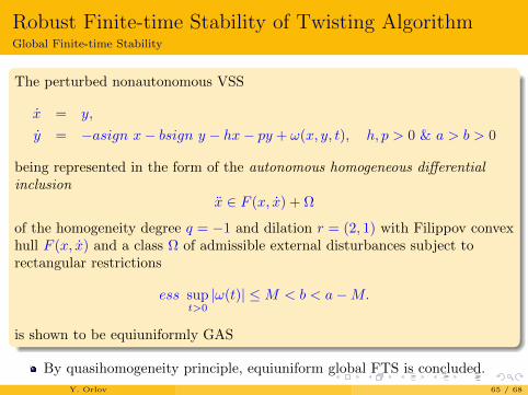
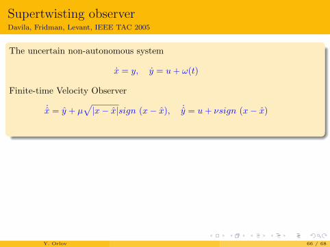
Supertwisting observerDavila, Fridman, Levant, IEEE TAC 2005
The uncertain non-autonomous system
x = y, y = u+ ω(t)
Finite-time Velocity Observer
˙x = y + µ√|x− x|sign (x− x), ˙y = u+ νsign (x− x)
The finite time error convergence e1 = x− x→ 0, e2 = y − y → 0 ast→∞ is guaranteed under uniform disturbance magnitude constraint
ess supt>0|ω(t)| ≤M < min
µ
2,µν
1 + µ
for some M > 0
The idea behind the velocity observer: the error dynamicse1 = e2 − µ
√|e1|sign e1, e2 = −νsign e1 + ω
are in the form of the FTS supertwisting algorithm.
Y. Orlov 66 / 68
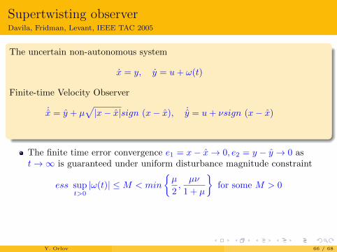
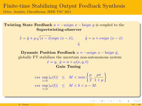
Finite-time Stabilizing Output Feedback SynthesisOrlov, Aoustin, Chevallereau, IEEE TAC 2011
Twisting State Feedback u = −asign x− bsign y is coupled to theSupertwisting-observer
˙x = y + µ√|x− x|sign (x− x), ˙y = u+ νsign (x− x)
⇓
Dynamic Position Feedback u = −asign x− bsign y,globally FT stabilizes the uncertain non-autonomous system
x = y, y = u+ ω(x, y, t)Gain Tuning
ess supt>0|ω(t)| ≤ M < min
µ
2,µν
1 + µ
ess sup
t>0|ω(t)| ≤ M < b < a−M.
Y. Orlov 67 / 68
Concluding RemarksOrlov Discontinuous Systems - Lyapunov Analysis and Robust Synthesis under UncertaintyConditions, Springer-Verlag, London, 2009
Analysis tools of discontinuous systems and sliding mode design methodsof the first and second orders were presented.
Capabilities of the methods and their robustness features were illustratedin mechanical applications
Y. Orlov 68 / 68


![Orlov ASPO2011 Planning[1]](https://img.pdfslide.us/doc/110x75/577d23241a28ab4e1e9914fa/orlov-aspo2011-planning1.jpg)