The yuima package: an R framework forsimulation and inference of stochastic

differential equations

Stefano Maria IacusDepartment of Economics, Business and Statistics

University of MilanVia Conservatorio 7, 20124 Milan, Italy

Abstract

The Yuima Project is an open source and collaborative effort ofseveral mathematicians and statisticians aimed at developing the $R$

package named “yuima” for simulation and inference of stochastic dif-ferential equations.

In the yuima package stochastic differential equations can be ofvery abstract type, e.g. uni or multidimensional, driven by Wienerprocess of fractional Brownian motion with general Hurst parameter,with or without jumps specified as L\’evy noise. L\’evy processes can bespecified via compound Poisson description, by the specification of theL\’evy measure or via increments and stable laws.

The yuima package is intended to offer the basic infrastructure onwhich complex models and inference procedures can be built on. In par-ticular, the basic set of functions includes the following: i) simulationschemes for all types of stochastic differential equations (Wiener, $fBm$,L\’evy); ii) different subsampling schemes including random samplingwith user specified random times distribution, space discretization, ticktimes, etc. iii) automatic asymptotic expansion for the approximationand estimation of functionals of diffusion processes with small noise viaMalliavin calculus, useful in option pricing; iv) efficient quasi-likelihoodinference for diffusion processes and model selection.

数理解析研究所講究録第 1752巻 2011年 85-112 85

1 IntroductionThe YUIMA Projectl is an open source2 academic project aimed at develop-ing the $R$ package named “yuima” for simulation and inference of stochasticdifferential equations. The YUIMA Project is mainly developed by mathe-maticians and statisticians who actively publish in the field of inference andsimulation for stochastic differential equations. The YUIMA Project CoreTeam, currently consists of the following people: A. Brouste, M. Fukasawa,H. Hino, S.M. Iacus, K. Kamatani, H.Masuda, Y. Shimizu, M. Uchida, N.Yoshida.

The yuima package provides an object-oriented programming environ-ment for simulation and statistical inference for stochastic processes by R.The yuima package adopts the S4 system of classes and methods (Chambers,1998).

Under this framework, the yuima package also supplies various functionsto execute simulation and statistical analysis. Both categories of proceduresmay depend each other. Statistical inference often requires a simulation tech-nique as a subroutine, and a certain simulation method needs to fix a tuningparameter by applying a statistical methodology. It is especially the case ofstochastic processes because most of expected values involved do not admit anexplicit expression. The yuima package facilitates comprehensive, systematicapproaches to the solution.

Stochastic differential equations are commonly used to model random evo-lution along continuous or practically continuous time, such as the randommovements of a stock price. Theory of statistical inference for stochastic dif-ferential equations already has a fairly long history, more than three decades,but it is still developing quickly new methodologies and expanding the area.The formulas produced by the theory are usually very sophisticated, whichmakes it difficult for standard users not necessarily familiar with this field toenjoy utilities. For example, the asymptotic expansion method for computingoption prices (i.e., expectation of an irregular functional of a stochastic pro-cess) provides precise approximation values instantaneously, taking advantageof the analytic approach, but the formula has a long expression like more thanone page!

The yuima package delivers up-to-date methods as a package onto the deskof the user working with simulation and/or statistics for stochastic differentialequations.

Sampled data from a continuous-time process features the time stamps aswell as the positions of the object. It is requiring a new theory of estimation.

lThe Project has been funded up to 2010 by the Japan Science Technology (JST) BasicResearch Programs PRESTO, Grants-in-Aid for Scientific Research No. 19340021.

2All code in the yuima package is subject to the GNU General Public License, Version2, see http: $//www$ . gnu. $org/$licenses$/gpl-2.0$ . html.

86

The yuima framework can apply multi-dimensional time stamps of tick dataand provides diverse functions handling such kind data to support statisticalanalysis.

Although we assume that the reader of this paper has a basic knowledgeof the $R$ language, most of the examples are easy to be understood by anyone.

2 The yuima packageThe package yuimna depends on some other packages, like zoo, which can beinstalled separately. The package zoo is used intemally to store time seriesdata. This dependence may change in the future adopting a more flexibleclass for internal storage of time series.

2.1 How to obtain the packageThe yuima package is hosted on R-Forge and the web page of the Project ishttp: $//r$-forge. r-project. org/projects/yuima. The R-Forge page con-tains the latest development version, and stable version of the package as alsoavailable through CRAN. Development versions of the package are not sup-posed to be stable or functional, thus the occasional user should consider toinstall the stable version first. The package can be instalIed $hom$ R-Forge usinginstall.packages (“ yuima”, repos $=”$ http $://R$ -Forge.R-proj ect. org”)and for the CRAN version, via install.packages(“ yuima”).

2.2 The main object and classesBefore discussing the methods for simulation and inference for stochastic pro-cesses solutions to stochastic differential equations, here we discuss the mainclasses in the package. As mentioned there are different classes of object de-fined in the yuima package and the main class is called the yuima-class andit is composed of several slots. Figure 1 represents the different classes andtheir slots. The different slots do not need to be all present at the same time.For example, in case one wants to simulate a stochastic process, only the slotsmodel and sampling should be present, while the slot data will be filled bythe simulator. We now discuss in details the different object separately.

2.3 The yuima.model classIn yuima three main classes of stochastic differential equations can be easilyspecified. All multidimensional and eventually as parametric models.

$\bullet$ diffusions $dX_{t}=a(t, X_{t})dt+b(t, X_{t})dW_{t}$ , where $W_{t}$ is a standard Brow-nian motion;

87

$\bullet$ fractional Gaussian noise, with $H$ the Hurst parameter

$dX_{t}=a(t, X_{t})dt+b(t, X_{t})dW_{t}^{H}$ ;

$\bullet$ diffusions with jumps and L\’evy processes solution to

$dX_{t}=a(X_{t})dt+b(X_{t})dW_{t}+\int_{|z|>1}c(X_{t-}, z)\mu(dt, dz)$

$+ \int_{0<|z|\leq 1}c(X_{t-}, z)\{\mu(dt, dz)-\nu(dz)dt\}$.

The yuima. model class contains informations about the stochastic differ-ential equation of interest. The constructor setModel is used to give a mathe-matical description of the stochastic differential equation. All functions in thepackage are assumed to get as much information as possible from the modelinstead of replicating the same code everywhere. If there are missing piecesof information, we may change or extend the description of the model.

An object of yuima. model contains several slots listed below. To see insideits structure, we use the $R$ command str.

$\bullet$ drift is an $R$ expression which contains the drift specification.

$\bullet$ diffusion is itself alist of 1 slot which describes the diffusion coefficientrelative to first noise.

$\bullet$ parameter which is a short name for “parameters” which is a list ofobjects.

$\bullet$ all contains the names of all the parameters found in the diffusion anddrift coefficient.

$\bullet$ common contains the names of the parameters in common between the.drift and diffusion coefficients.

$\bullet$ diffusion contains the parameters belonging to the diffusion coeffi-cient.

$\bullet$ drift contains the parameters belonging to the drift coefficient.

$\bullet$ solve. variable contains a vector of variable names, each element cor-responds to the name of the solution variable (left-hand-side) of eachequation in the model, in the corresponding order.

88

$\bullet$ state. variable and time. variable, by default, are assumed to be $x$

and $t$ but the user can freely choose them. The yuima. model functionassumes that the user either use default names for state. variable andtime. variable variables or specify his own names. All the rest of thesymbols are considered parameters and distributed accordingly in theparameter slot.

$\bullet$ noise. number indicates the number of sources of noise.

$\bullet$ equation. number represents the number of equations, i.e. the numberof one dimensional stochastic differential equations.

$\bullet$ dimension reports the dimensions of the parameter space. It is a list ofthe same length of parameter with the same names.

In order to show how general is the approach in the yuima package wepresent some examples.

2.3.1 Diffusion processes

Assume that we want to describe the following stochastic differential equation

$dX_{t}=-3X_{t}dt+\frac{1}{1+X_{t}^{2}}dW_{t}$

This is done in yuima specifying the drift and diffusion coefficients as plainmathematical expressions

$R>modl$ $<-setMo$del (drift $=$ $-3*x’$‘,$+$ $di$ffusion $=$ $|l/(1+x^{\sim}2)$ “ $)$

At this point, the package fills the proper slots of the yuima object$R>$ str (modl)

Formal class ’yuima.model‘ [package “yuima“] with 16 slots$Q$ drift : expression $((-3*x))$

. .@ diffusion :List of 1

. . . .$: expression $(l/(l +x^{-}2))$@ hurst : num 0.5

. .@jump. coeff : expression $()$

. . $Q$ measure : list $()$

. .6 measure. type : chr(0)

. . @ parameter : Formal class model. parameter $t$ [package “ yuima“] with 6 slots. , @ all : chr(0). .

. . . . $\emptyset$ common : chr(0)

. . . . . . $Q$ diffusion: chr(0)

. .@ drift : chr(0). .. . . . . .@ jump : chr(0)

. . $Q$ measure : chr(0). .$\Phi$ state.variable: chr $x”$

. . $Q$ jump.variable : chr(0)

. . $Q$ time. variable : chr $|t^{\prime 1}$

. . $Q$ noise.number ; num 1

89

. .0 equation.number: int 1$Q$ dimension : int [1:610 $00000$$Q$ solve.variable : chr $x”$

. . $Q$ xinit : num $0$

. . $Q$ J. flag : logi FALSE

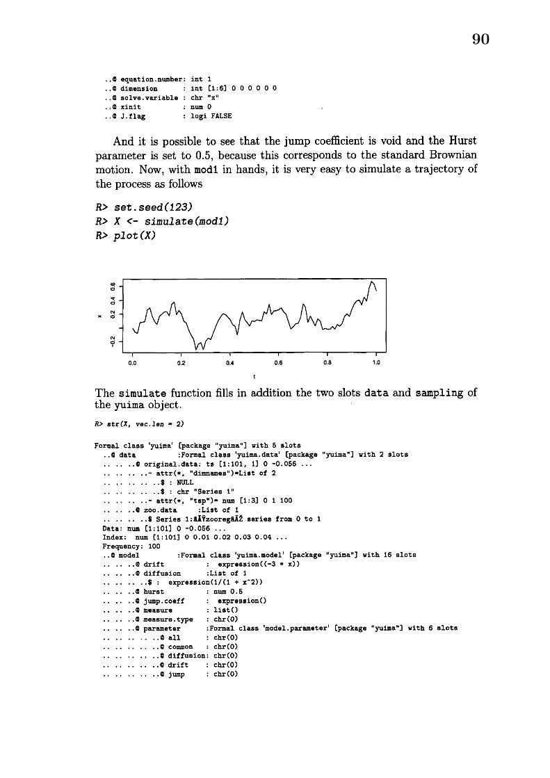
And it is possible to see that the jump coefficient is void and the Hurstparameter is set to 0.5, because this corresponds to the standard Brownianmotion. Now, with modl in hands, it is very easy to simulate a trajectory ofthe process as follows

$R>$ set. seed (123)

$R>X<$-simulate (modl)

$R>plot$ (X)

0.0 02 0.4 06 0.8 1.0

$t$

The simulate function fills in addition the two slots data and sampling ofthe yuima object.$R>$ str (X, vec. 1 en $=2$)

Formal class yuima‘ [package $|yuima^{1\mathfrak{l}}$ ] with 5 slots$Q$ data :Formal class ‘yuima.data‘ [package “yuima”] with 2 slots

. . $Q$ original. data; ts [1: 101. 1] $0$ -0.056 . . .. .. . . . . . . $.-$ attr( $*,$ dimames) $\cdot List$ of 2

. . . . . .$: NULL. .. . . . . . . . . .$: chr “Series 1 “

. . . . . . . $.-$ attr $(*, tsp)-$ num [1:3] 01100$Q$ zoo.data :List of 1. .

. .$ Series 1: $g\ddot{Y}zooregil2$ series from $0$ to 1. .Data; num [1; 101] $0$ -0.056 . . .Index: num [1:101] $0$ 0.010.02 0.03 0.04 . . .Frequency; 100. . $Q$ model : Formal class ’yuima. model‘ [package “yuima”] with 16 slots

$Q$ drift : expression$((-3*x))$. .. . . . $Q$ diffusion :List of 1. . . . . . . .$: expression$(l/(l +x2))$

$Q$ hurst : num 0.5. .. . . . $Q$ jump. coeff : expression $()$

$Q$ measure : list $()$. .. . . . . . $Q$ measure. type : chr(0)

. . $Q$ parameter : Formal class ’model. paramoter’ [package ”yuima”] with 6 slots. .. . . . . . . . . . $Q$ all : chr(0)

. . . . . . . . $\Phi$ common : chr(0)

. . . . . . . , . . $Q$ diffusion: chr(0)

. . . . . . . . . . $Q$ drift : chr(0)

. . . . . . . . $Q$ jump : chr(0)

90

. . . . . . . . . . $Q$ measure ; chr(0)

. . . . $\emptyset$ state.variable: chr )$t|x$’

. . $Q$ jump.variable : chr(0)

. . . . . .6 $t$ ime.variable ; chr ${}^{t}t’$

. . . . . .@ noise.number : num 1

. . . . . .@equation.number: int 1

. . . . $Q$ dimension : int [1;6] $00000$ . . .$Q$ solve.variable ; chr $x^{I1}$. .

. . . . . .@ xinit : num $0$

. . $Q$ J. flag ; logi FALSE$Q$ sampling :Formal class yuima.sampling‘ [package ”yuima“] with 11 slots

$Q$ Initial : num $0$. .. . . . $\Phi$ Terminal : num 1. . . . $Qn$ ; num 100. . . . . . $Q$ delta : num 0.01. . . . $Q$ grid :List of 1

. .$: num [1:101] $0$ 0.010.02 0.03 0.04 . . .. .. . . . . .@ random ; logi FALSE. . . . $\emptyset$ regular : logi TRUE. . . . . .@sdelta : num(0)

. .@ sgrid : num(0). .. . . . $Q$ oindex : num(0)

. . $Q$ interpolation: chr “pt’t$Q$ characteristic:Formal class $|yuima.characteristic$ ’ [package ”yuima“] with 2 slots

. . $\mathfrak{g}$ equation.number; int 1. .@ time.scale : num 1. .

. . $Q$ functional : Formal class lyuima. functional ‘ [package “ yuima”] with 4 slots. , $QF$ : NULL. .

. . . . . .6 $f$ $:1ist()$

. . . . $\emptyset$ xinit: num(0). . Qe : num(0). .

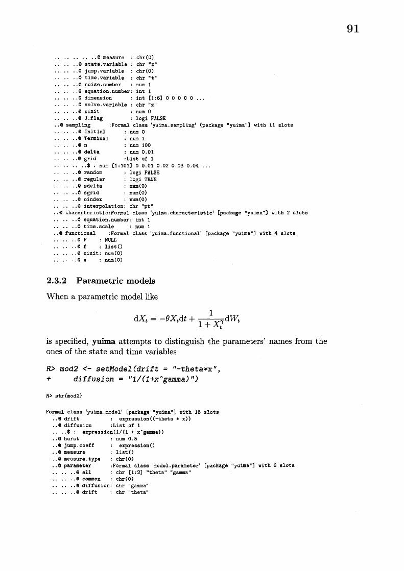
2.3.2 Parametric models

When a parametric model like

$dX_{t}=-\theta X_{t}dt+\frac{1}{1+X_{t}^{\gamma}}dW_{t}$

is specified, yuima attempts to distinguish the parameters’ names from theones of the state and time variables

$R>mod2$ $<-setModel(drift=$ $”-theta*x”$ ,$+$ $dif$fusi on $=$ “ $1/(1+x^{-}gamma)$ “ $)$

$R\succ$ str (mod2)

Formal class yuima.modelt [package ‘yuima“] with 16 slots$\Phi$ drift : expression((-theta $*x)$ )

. . $Q$ diffusion :List of 1

. . . .$: expression(l/(l $+x^{-}$gamma$)$ )

. . $G$ hurst : num 0.5

. . $Q$ jump.coeff : expression $()$

. . $Q$ measure : list $()$

. . $Q$ measure. type ; chr(0)

. . $Q$ parameter : Formal class model. parameter $|$ [package ”yuima”] with 6 slots. . $\Phi$ all ; chr [1 : 2] $1\dagger$ thet $a^{11}$ “gamma”. .. . @ common : chr(0). .

. . . . . . $Q$ diffusion; chr ”gamma“$\Phi$ drift : chr 1ltheta”. .

91

. . . . $Q$ jump : chr(0)

. . $Q$ measure : chr(0). .$Q$ state.variable: chr $x^{1\prime}$

. .9 jump.variable : chr(0)

. . $Q$ time.variable : chr $t$ “

$Q$ noise.number : num 1. . $Q$ equation.number: int 1

$Q$ dimension : int [1:6] 2 0110 $0$

. . $Q$ solve. variable : chr $x”$

. . $Q$ xinit : num $0$

$Q$ J.flag ; logi FALSE

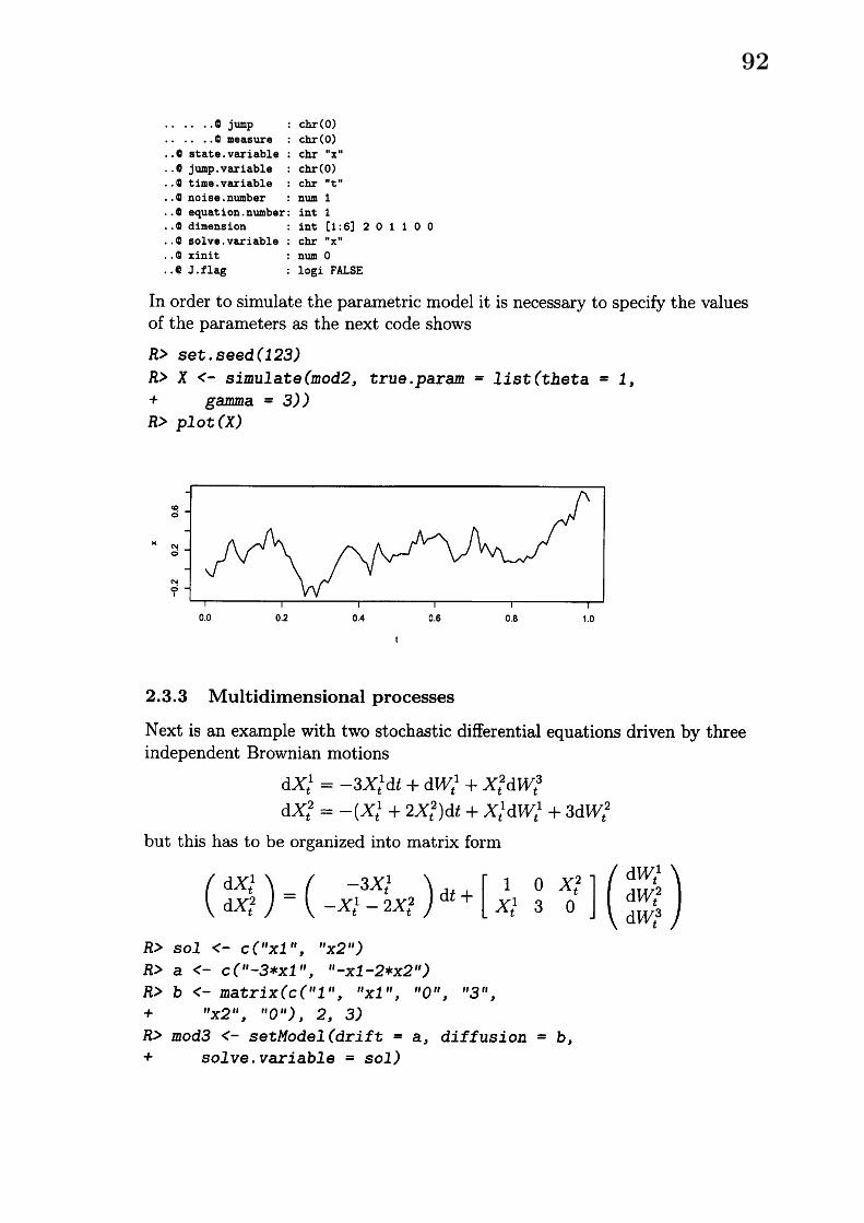
In order to simulate the parametric model it is necessary to specify the valuesof the parameters as the next code shows$R>set.$ seed (123)

$R>X<$-simulate (mod2, true. par$am=list$ (theta $=1$ ,$+$ gamma $=3$) $)$

$R>plot$ (X)

0.0 02 04 06 08 10

$t$

2.3.3 Multidimensional processes

Next is an example with two stochastic differential equations driven by threeindependent Brownian motions

$dX_{t}^{1}=-3X_{t}^{1}dt+dW_{t}^{1}+X_{t}^{2}dW_{t}^{3}$

$dX_{t}^{2}=-(X_{t}^{1}+2X_{t}^{2})dt+X_{t}^{1}dW_{t}^{1}+3dW_{t}^{2}$

but this has to be organized into matrix form

$(dX_{t}^{2}dX_{t}^{1})=(\begin{array}{l}-3X_{t}^{l}--X_{t}^{1}2X_{t}^{2}\end{array})dt+\{\begin{array}{lll}1 0 X_{t}^{2}X_{t}^{1} 3 0\end{array}\}(dW_{t}^{3}dW_{t}^{2}dW_{t}^{1})$

$R>sol<-c(^{\prime l}x1’’$ , “x2 “ $)$

$R>$ a $<-c$ $(”-3*xl ”, ”-xl-2*x2”)$$R>b<$-matrix $(c(^{ll}l$ ”, $xl$ ”, $0^{l\prime}$ , $3^{\prime l}$ ,$+$ $x2^{\iota\prime}$ , $|0’’),$ $2,3)$$R>mod3$ $<$-setModel (dri$ft=a,$ $di$ffusion $=b$ ,$+$ $solve$ . vari$able=sol$)

92

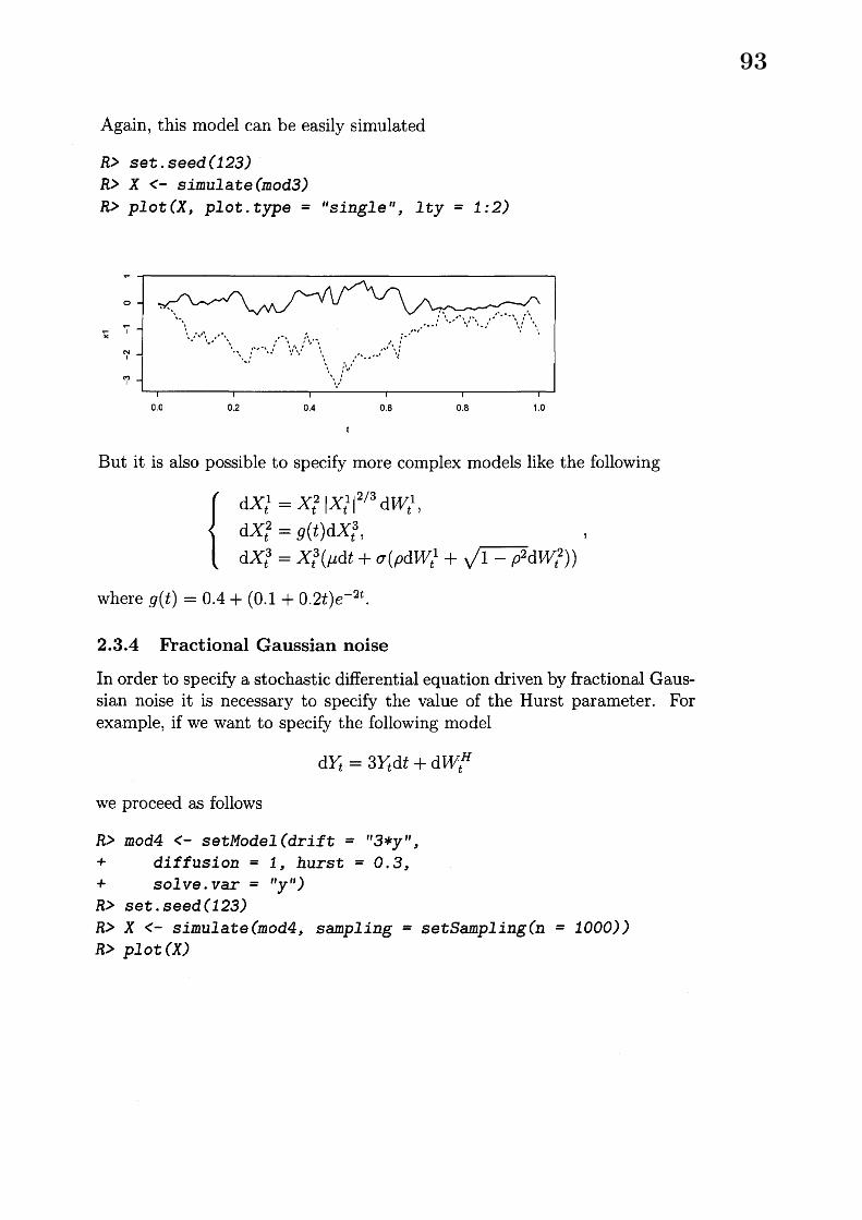
Again, this model can be easily simulated

$R>$ set. seed (123)

$R>X<-simul$ate (mod3)

$R>plot$ (X, plot. type $=$ “si$ngle^{t},$ $lty=1:2$)

00 02 04 0.6 08 10

1

But it is also possible to specify more complex models like the following

$\{\begin{array}{l}dX_{t}^{1}=X_{t}^{2}|X_{t}^{1}|^{2/3}dW_{t}^{1},dX_{t}^{2}=g(t)dX_{t}^{3}, ,dX_{t}^{3}=X_{t}^{3}(\mu dt+\sigma(\rho dW_{t}^{1}+\sqrt{1-\rho^{2}}dW_{t}^{2}))\end{array}$

where $g(t)=0.4+(0.1+0.2t)e^{-2t}$ .

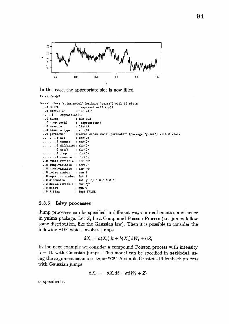
2.3.4 Fractional Gaussian noise

In order to specify a stochastic differential equation driven by fractional Gaus-sian noise it is necessary to specify the value of the Hurst parameter. Forexample, if we want to specify the following model

$dY_{t}=3Y_{t}dt+dW_{t}^{H}$

we proceed as follows

$R>mo$d4 $<-s$ etModel $(drift=$ “$3*y^{l\prime}$ ,

$+$ diffusion $=1$ , hurst $=0.3$ ,$+$ solve. $var=|y\uparrow’)$

$R>set.$ seed (123)

$R>X<$-simulate (mod4, sampling $=$ setSampli$ng(n=1000)$ )

$R>plot$ (X)

93

00 02 0.4 06 0.8 10

$t$

In this case, the appropriate slot is now filled$R\succ str(mod4)$

Formal class yuima.model ‘ [package “yuima”] with 16 slots. . $Q$ drift ; expression$((3 *y))$. . $Q$ diffusion : List of 1. . . .$: expression(l). . $Q$ hurst : num 0.3. . $Q$ jump. coeff : expression $()$

. . $\emptyset$ measure : list $()$

. . $Q$ measure.type : chr(0)

. . $Q$ parameter ; Formal class ‘model. parametert [package “yuima”] with 6 slots$Q$ all ; chr(0). .

. . . . $Q$ common : chr(0)

. . . . . .0 diffusion: chr(0)

. . . . $Q$ drift : chr(0). . $Q$ jump : chr(0)

. . $Q$ measure ; chr(0). .. . $Q$ state.variable: chr $x”$

$Q$ jump.variable : chr(0)$Q$ time. variable : chr $t^{\prime\iota}$

$Q$ noise.number : num 1$Q$ equation.number: int 1

. . $Q$ dimension ; int [1:6] $000000$$Q$ solve.variable; chr $|\prime y’’$

$Q$ xinit : num $0$

$Q$ J. flag ; logi FALSE

2.3.5 L\’evy processes

Jump processes can be specified in different ways in mathematics and hencein yuima package. Let $Z_{t}$ be a Compound Poisson Process (i.e. jumps followsome distribution, like the Gaussian law). Then it is possible to consider thefollowing SDE which involves jumps

$dX_{t}=a(X_{t})dt+b(X_{t})dW_{t}+dZ_{t}$

In the next example we consider a compound Poisson process with intensity$\lambda=10$ with Gaussian jumps. This model can be specified in setModel us-ing the argument measure. type$=t\dagger$ CP $11$ A simple Ornstein-Uhlembeck processwith Gaussian jumps

$dX_{t}=-\theta X_{t}dt+$ ad$W_{t}+Z_{t}$

is specified as

94

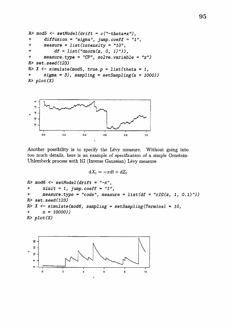
$R>mod5$ $<-$ se$tModel(drift=c$ $(”-theta*x^{t\prime})$ ,$+$ diffusion $=$ sigm$a^{l1}$ , jump. coeff $=$ “1 “,$+$ measure $=list$ (intensity $=\prime\prime 10$ “,$+$ $df=list$ (”dnorm ($z,$ $0$ , I) “) $)$ ,$+$ measure. $type=$ “ $CP$ “, $solve$ . vari $able=\iota_{X^{l\dagger)}}$

$R>set.$ seed (123)

$R>X<$-simulate (mod5, tru$e.p=list$ (theta $=1$ ,$+$ $si$gma $=3$), $s$ampl$ing=s$etSampl $ing(n=1000))$$R>plot$ (X)

0.0 02 0.4 0.6 0.8 10

$t$

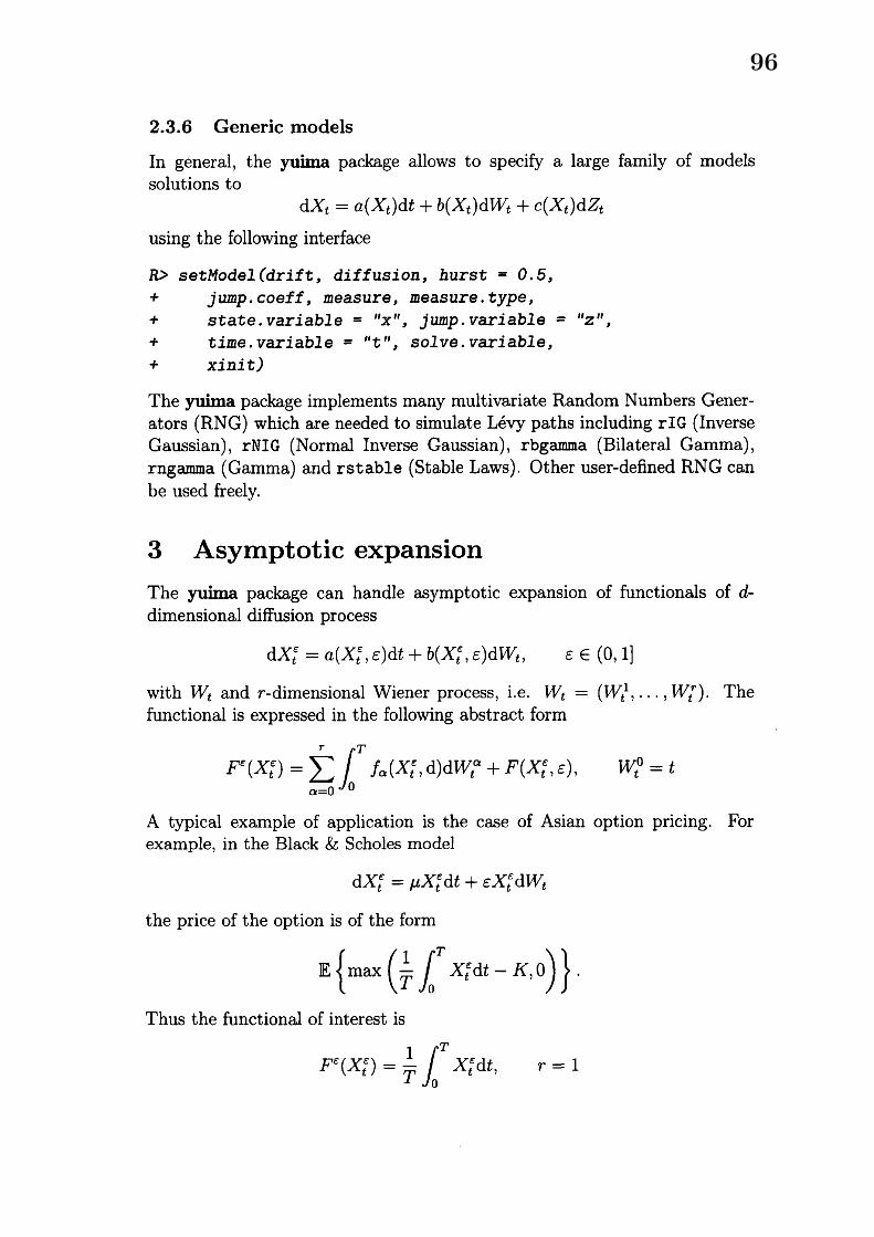
Another possibility is to specify the L\’evy measure. Without going intotoo much details, here is an example of specification of a simple Ornstein-Uhlembeck process with IG (Inverse Gaussian) L\’evy measure

$dX_{t}=-xdt+dZ_{t}$

$R>mod6$ $<$-setModel $(drift=$ $”-x^{\prime 1}$ ,$+$ xinit $=1,$ $j$ ump. coeff $=$ “ 1 “,$+$ measure. $type=$ “code“, measure $=list$ $(df=||r\mathcal{I}G(z, 1,0.1) "))$

$R>set.$ seed (I23)

$R>X<$-simulate (mod6, sampling $=$ setSampl $ing$ (Terminal $=10$ ,$+$ $n=1$ 0000$))$

$R>plot$ (X)

$0$ 2 4 6 8 40

1

95

2.3.6 Generic models

In general, the yuima package allows to specify a large family of modelssolutions to

$dX_{t}=a(X_{t})dt+b(X_{t})dW_{t}+c(X_{t})dZ_{t}$

using the following interface

$R>$ setModel $(drift,$ $di$ffusion, hurst $=0.5$ ,$+$ jump. coeff, measure, measure. type,$+$ $st$ a$te$ . vari a$ble=$ $x”$ , jump. vari a$ble=\iota\prime z^{l\prime}$ ,$+$ $time$ . vari a$ble=$ $|t$ “, solve. vari a$ble$ ,$+$ $xi$nit)

The yuima package implements many multivariate Random Numbers Gener-ators (RNG) which are needed to simulate L\’evy paths including $rIG$ (InverseGaussian), $rNIG$ (Normal Inverse Gaussian), rbgamma (Bilateral Gamma),rngamma (Gamma) and rstabIe (Stable Laws). Other user-defined RNG canbe used freely.

3 Asymptotic expansionThe yuima package can handle asymptotic expansion of functionals of d-dimensional diffusion process

$dX_{t}^{\epsilon}=a(X_{t}^{\epsilon}, \epsilon)dt+b(X_{t}^{\epsilon}, \epsilon)dW_{t}$ , $\epsilon\in(0,1]$

with $W_{t}$ and r-dimensional Wiener process, i.e. $W_{t}=(W_{t}^{1}, \ldots, W_{t}^{r})$ . Thefunctional is expressed in the following abstract form

$F^{\epsilon}(X_{t}^{\epsilon})= \sum_{\alpha=0}^{r}\int_{0}^{T}f_{\alpha}(X_{t}^{\epsilon}, d)dW_{t}^{\alpha}+F(X_{t}^{\epsilon}, \epsilon)$ , $W_{t}^{0}=t$

A typical example of application is the case of Asian option pricing. Forexample, in the Black & Scholes model

$dX_{t}^{\epsilon}=\mu X_{t}^{\epsilon}dt+\epsilon X_{t}^{\epsilon}dW_{t}$

the price of the option is of the form

$E\{\max(\frac{1}{T}\int_{0}^{T}X_{t}^{\epsilon}dt-K,$ $0)\}$ .

Thus the functional of interest is

$F^{\epsilon}(X_{t}^{\epsilon})= \frac{1}{T}\int_{0}^{T}X_{t}^{\epsilon}dt$ , $r=1$

96

with$f_{0}(x, \epsilon)=\frac{x}{T}$ , $f_{1}(x, \epsilon)=0$ , $F(x, \epsilon)=0$

in

$F^{\in}(X_{t}^{\epsilon})= \sum_{\alpha=0}^{r}\int_{0}^{T}f_{\alpha}(X_{t}^{\epsilon}, d)dW_{t}^{\alpha}+F(X_{t}^{\epsilon}, \epsilon)$

So, the call option price requires the composition of a smooth functional

$F^{\epsilon}(X_{t}^{\epsilon})= \frac{1}{T}\int^{T}X_{t}^{\epsilon}dt$ , $r=1$

with the irregular function

$\max(x-K, 0)$

Monte Carlo methods require a huge number of simulations to get the desiredaccuracy of the calculation of the price, while asymptotic expansion of $F^{\epsilon}$ pro-vides very accurate approximations. The yuima package provides functionsto construct the functional $F^{\epsilon}$ , and automatic asymptotic expansion based onMalliavin calculus starting from a yuima object. Next is an example$R>diff$ . matrix $<$-matrix $(c(^{ll}x*e^{\prime\downarrow})$ ,$+$ 1, 1)$R>$ model $<-setModel$ (drift $=c(\prime\prime x’’)$ ,$+$ diffusion $=diff$ . matrix)

$R>T<-1$$R>$ xinit $<-1$

$R>K<-1$$R>f<$-list (expression(x/T), expression (0))

$R>F<-0$$R>e<-O.3$$R>$ yuima $<$-setYuima (model $=$ model,$+$ sampling $=setSampling$ (Terminal $=T$,$+$ $n=1000))$$R>yu$ ima $<$-setFunction$al$ (yuima, $f=f$ ,$+$ $F=F$, xinit $=$ xinit, $e=e$)

this time the setFunctional command fills the appropriate slots$R>$ str(yuima@function$al$ )

FormaI class ‘yuima. functional‘ [package “yuimail] with 4 slots. .@ $F$ : num $0$

. .@f :List of 2

. . . .$: expression(x/T)

. . . .$: expression(0)

. .@ xinit: num 1

. .@ $e$ : num 0.3

97

Then, it is as easy as

$R>FO<-FO$ (yuima)$R>FO$

[1] 1. 717423

$R> \max(FO-K, 0)$

[1] $0$ . 7174228

to obtain the zero order approximation of the value of the functional. We cango up to the first order approximation adding one term to the expansion

$R>rho<$-expressi on (0)

$R>get- ge<-f$unction $(x$ , epsilon,$+$ $K,$ $F0)$ $\{$

$+$ $tmp<-(FO-K)+$ (epsilon $*$

$+$ x$)$

$+$ $tmp[$(epsilon $*x$) $<(K-F0)J<-0$$+$ return $(tmp)$

$+\}$

$R>$ epsilon $<-e$

$R>g<-f$unction (x) {$+$ $tmp<-(FO-K)+$ (epsilon $*$

$+$ x$)$

$+$ $tmpf$(epsi1on $*x$) $<(K-FO)J<-0$$+$ $tmp$

$+\}$

$R>$ asymp $<-a$sympt$otic_{-}term$ (yuima,$+$ $block=10,$ $rho$ , g$)$

and the final value is

$R>$ asymp$dO $+e*$ asymp$d1

[1] $0$ . 7158789

4 Quasi Maximum Likelihood estimationConsider the multidimensional diffusion process

$dX_{t}=b(\theta_{2}, X_{t})dt+\sigma(\theta_{1}, X_{t})dW_{t}$

98

where $W_{t}$ is an r-dimensional standard Wiener process independent of theinitial value $X_{0}=x_{0}$ . Quasi-MLE assumes the following approximation ofthe true log-likelihood for multidimensional diffusions

$\ell_{n}(X_{n}, \theta)=-\frac{1}{2}\sum_{i=1}^{n}\{\log\det(\Sigma_{i-1}(\theta_{1}))+\frac{1}{\triangle_{n}}\Sigma_{i-1}^{-1}(\theta_{1})[\Delta X_{i}-\triangle_{n}b_{i-1}(\theta_{2})]^{\otimes 2}\}(4.1)$

where $\theta=(\theta_{1}, \theta_{2}),$ $\triangle X_{i}=X_{t_{i}}-X_{t_{i-1}},$ $\Sigma_{i}(\theta_{1})=\Sigma(\theta_{1}, X_{t_{i}}),$ $b_{i}(\theta_{2})=b(\theta_{2}, X_{t_{:}})$ ,$\Sigma=\sigma^{\otimes 2},$ $A^{\otimes 2}=A^{T}A$ and $A^{-1}$ the inverse of $A,$ $A[B]^{\otimes 2}=B^{T}AB$ . Then,Yoshida (1992), the QML estimator of $\theta$ is

$\tilde{\theta}_{n}=\arg\min_{\theta}l_{n}(X_{n}, \theta)$

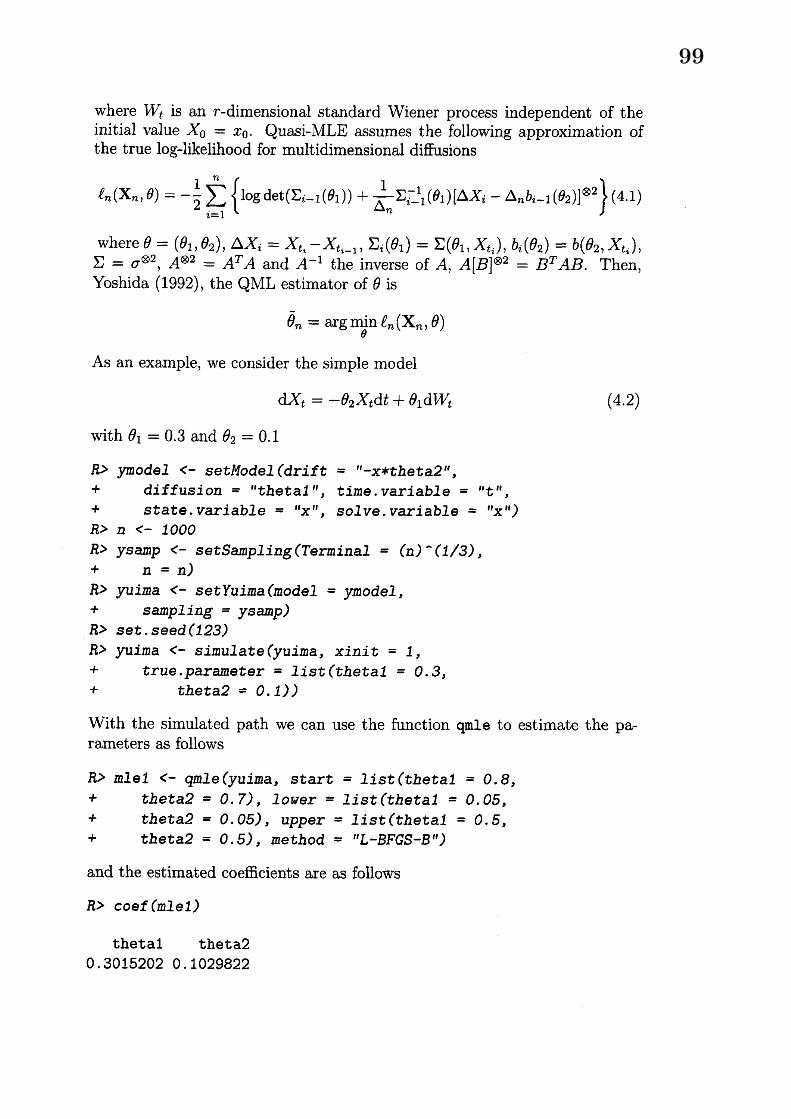
As an example, we consider the simple model

$dX_{t}=-\theta_{2}X_{t}dt+\theta_{1}dW_{t}$ (4.2)

with $\theta_{1}=0.3$ and $\theta_{2}=0.1$

$R>$ ymodel $<$-setModel (dri$ft=$ $”-x*thet$a2 “,$+$ diffusion $=$ “thetal “, time. variable $=$ $|t^{ll}$ ,$+$ state. variable $=\uparrow\prime x^{l\prime},$ $solve$ . var$i$ a$ble={}^{t}x’’$)$R>11<-\iota 000$

$R>$ ysamp $<$-setSampling (Terminal $=(n)^{\sim}(1/3)$ ,$+$ $n=n)$$R>$ yuima $<$-setYuima (model $=ym$odel,$+$ $s$ampl$ing=ys$amp)$R>set.$ seed (123)

$R>yuima<$-simulate $(yuima$ , xinit $=1$ ,$+$ true. paramet$er=list$ (thetal $=0.3$ ,$+$ $th$eta2 $=0.1$ ) $)$

With the simulated path we can use the function qmle to estimate the pa-rameters as follows

$R>mlel$ $<-qmle(yuima$ , start $=list$ (thetal $=0.8$ ,$+$ theta2 $=0.7$), $lower=list$ (th$etal=0.05$ ,$+$ $th$eta2 $=0.05$), upper $=list$ (thetal $=0.5$ ,$+$ theta2 $=0.5$) , me $thod=\mathfrak{l}|L-BFGS-B$ “ $)$

and the estimated coefficients are as follows

$R>$ coef $(mlel)$

thetal theta20.3015202 0.1029822

99

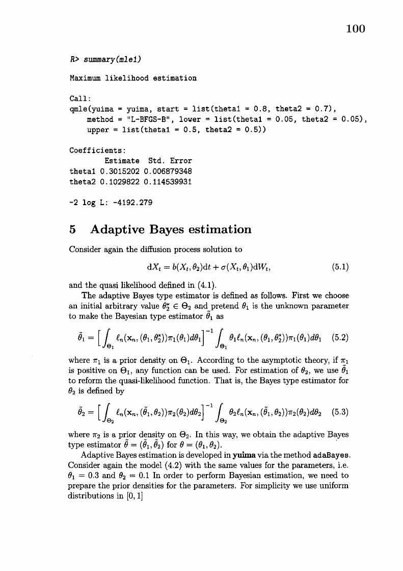
$R>s$ummary $(mlel)$

Maximum likelihood estimation

CalI:qmle (yuima $=$ yuima, start $=$ list (thetal $=0.8$ , theta2 $=0.7$),

method $=||L-BFGS-B^{11}$ , lower $=$ list (thetal $=0.05$ , theta2 $=0.05$),

upper $=$ list (thetal $=0.5$ , theta2 $=0.5$) $)$

Coefficients:Estimate Std. Error

theta10.30152020.006879348theta2 0.1029822 0.114539931

$-2\log L:-4192.279$

5 Adaptive Bayes estimationConsider again the diffusion process solution to

$dX_{t}=b(X_{t}, \theta_{2})dt+\sigma(X_{t}, \theta_{1})dW_{t}$ , (5.1)

and the quasi likelihood defined in (4.1).The adaptive Bayes type estimator is defined as follows. First we choose

an initial arbitrary value $\theta_{2}^{\star}\in\Theta_{2}$ and pretend $\theta_{1}$ is the unknown parameterto make the Bayesian type estimator $\tilde{\theta}_{1}$ as

$\tilde{\theta}_{1}=[\int_{\Theta_{1}}\ell_{n}(x_{\eta}, (\theta_{1}, \theta_{2}^{\star}))\pi_{1}(\theta_{1})d\theta_{1}]^{-1}\int_{\Theta_{1}}\theta_{1}\ell_{n}(x_{n}, (\theta_{1}, \theta_{2}^{\star}))\pi_{1}(\theta_{1})d\theta_{1}$ (5.2)

where $\pi_{1}$ is a prior density on $\Theta_{1}$ . According to the asymptotic theory, if $\pi_{1}$

is positive on $\Theta_{1}$ , any function can be used. For estimation of $\theta_{2}$ , we use $\tilde{\theta}_{1}$

to reform the quasi-likelihood function. That is, the Bayes type estimator for$\theta_{2}$ is defined by

$\tilde{\theta}_{2}=[\int_{\Theta_{2}}l_{n}(x_{n}, (\tilde{\theta}_{1}, \theta_{2}))\pi_{2}(\theta_{2})d\theta_{2}]^{-1}\int_{\Theta_{2}}\theta_{2}l_{n}(x_{n}, (\tilde{\theta}_{1}, \theta_{2}))\pi_{2}(\theta_{2})d\theta_{2}$ (5.3)

where $\pi_{2}$ is a prior density on $\Theta_{2}$ . In this way, we obtain the adaptive Bayestype estimator $\tilde{\theta}=(\tilde{\theta}_{1},\tilde{\theta}_{2})$ for $\theta=(\theta_{1}, \theta_{2})$ .

Adaptive Bayes estimation is developed in yuima via the method adaBayes.Consider again the model (4.2) with the same values for the parameters, i.e.$\theta_{1}=0.3$ and $\theta_{2}=0.1$ In order to perform Bayesian estimation, we need toprepare the prior densities for the parameters. For simplicity we use uniformdistributions in $[0,1]$

100

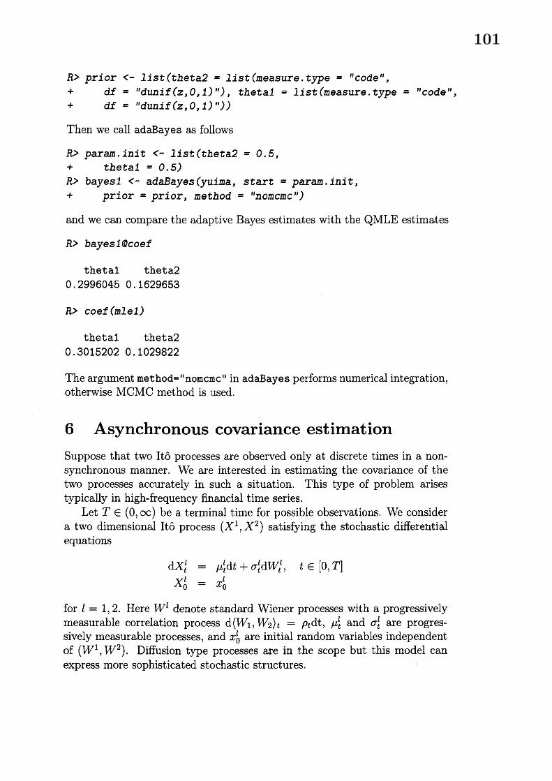
$R>prior<$-list (theta2 $=list$ (measure. $type=ll$ cod$e^{}$ ,$+$ $df=$ $d$uni$f(z, 0,1)$ “ $)$ , $th$etal $=list$ (measure. type $=ll$ code“,$+$ $df=$ “dun$if(z, 0,1)^{ll}))$

Then we call adaBayes as follows

$R>p$aram. init $<$-list (theta2 $=0.5$ ,$+$ $th$eta 1 $=0.5$)$R>$ baye$s1<-adaBayes$ (yuima, start $=p$ararn. $init$ ,$+$ prior $=$ prior, method $=$ “nomcmc“)

and we can compare the adaptive Bayes estimates with the QMLE estimates

$R>$ bayesl @coe$f$

thetal theta20.2996045 0.1629653

$R>$ coef $(mlel)$

thetal theta20.30152020.1029822

The argument method$=^{t\mathfrak{l}}$ nomcm$c^{1I}$ in adaBayes performs numerical integration,otherwise MCMC method is used.

6 Asynchronous covariance estimationSuppose that two It\^o processes are observed only at discrete times in a non-synchronous manner. We are interested in estimating the covariance of thetwo processes accurately in such a situation. This type of problem arisestypically in high-frequency financial time series.

Let $T\in(O, \infty)$ be a terminal time for possible observations. We considera two dimensional It\^o process $(X1, X^{2})$ satisfying the stochastic differentialequations

$dX_{t}^{l}$ $=$ $\mu_{t}^{l}dt+\sigma_{t}^{l}dW_{t}^{l}$ , $t\in[0, T]$

$X_{0}^{l}$ $=$ $x_{0}^{l}$

for $l=1,2$ . Here $W^{l}$ denote standard Wiener processes with a progressivelymeasurable correlation process $d\langle W_{1},$ $W_{2}\rangle_{t}=\rho_{t}$dt, $\mu_{t}^{l}$ and $\sigma_{t}^{l}$ are progres-sively measurable processes, and $x_{0}^{l}$ are initial random variables independentof $(W^{1}, W^{2})$ . Diffusion type processes are in the scope but this model canexpress more sophisticated stochastic structures.

101

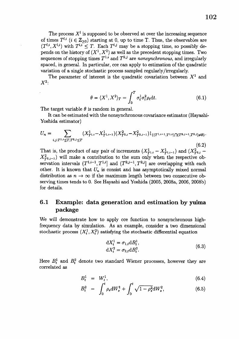
The process $X^{l}$ is supposed to be observed at over the increasing sequenceof times $T^{l,i}(i\in \mathbb{Z}_{\geq 0})$ starting at $0$ , up to time T. Thus, the observables are$(T^{l,i}, X^{l,i})$ with $T^{l,i}\leq T$ . Each $T^{l,j}$ may be a stopping time, so possibly de-pends on the history of $(X1, X^{2})$ as well as the precedent stopping times. Twosequences of stopping times $T^{1,i}$ and $T^{2,j}$ are nonsynchronous, and irregularlyspaced, in general. In particular, cce can apply to estimation of the quadraticvariation of a single stochastic process sampled regularly/irregularly.

The parameter of interest is the quadratic covariation between $X^{1}$ and$X^{2}$ :

$\theta=\langle X^{1},$ $X^{2} \rangle_{T}=\int_{0}^{T}\sigma_{t}^{1}\sigma_{t}^{2}\rho_{t}dt$ . (6.1)

The target variable $\theta$ is random in general.It can be estimated with the nonsynchronous covariance estimator (Hayashi-

Yoshida estimator)

$U_{n}= \sum_{i,j:T^{1,i}\leq T,T^{2,j}\leq T}(X_{T^{1}}^{1},.-X_{T^{1.i-1}}^{1})(X_{T^{2,j}}^{2}-X_{T^{2,j-1}}^{2})1_{\{(T^{1,i-1},T^{1,i}]\cap(T^{2,j-1},T^{2,j}]\neq\emptyset\}}$.

That is, the product of any pair of increments $(X_{T^{1}}^{1},$ . $-X_{T^{1,i-1}}^{1})$ and$(X_{T^{2,j}}^{2}-(62)$

$X_{T^{2,j-1}}^{2})$ will make a contribution to the sum only when the respective ob-servation intervals $(T^{1,i-1}, T^{1,i}]$ and $(T^{2,j-1}, T^{2,j}]$ are overlapping with eachother. It is known that $U_{n}$ is consist and has asymptotically mixed normaldistribution as $narrow\infty$ if the maximum length between two consecutive ob-serving times tends to $0$ . See Hayashi and Yoshida $(2005, 2008a, 2006, 2008b)$for details.

6.1 Example: data generation and estimation by yuimapackage

We will demonstrate how to apply cce function to nonsynchronous high-frequency data by simulation. As an example, consider a two dimensionalstochastic process $(X_{t}^{1}, X_{t}^{2})$ satisfying the stochastic differential equation

$dX_{t}^{1}=\sigma_{1,t}dB_{t}^{1}$ ,(6.3)

$dX_{t}^{2}=\sigma_{2,t}dB_{t}^{2}$ .

Here $B_{t}^{1}$ and $B_{t}^{2}$ denote two standard Wiener processes, however they arecorrelated as

$B_{t}^{1}$ $=$ $W_{t}^{1}$ , (6.4)

$B_{t}^{2}$ $=$ $\int_{0}^{t}\rho_{s}dW_{s}^{1}+\int_{0}^{t}\sqrt{1-\rho_{s}^{2}}dW_{s}^{2}$, (6.5)

102

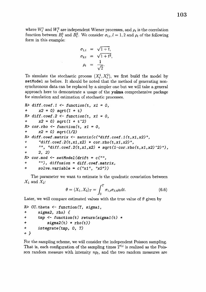
where $W_{t^{1}}$ and $W_{t}^{2}$ are independent Wiener processes, and $\rho_{t}$ is the correlationfunction between $B_{t}^{1}$ and $B_{t}^{2}$ . We consider $\sigma_{l,t},$ $l=1,2$ and $\rho_{t}$ of the followingform in this example:

$\sigma_{1,t}$ $=$ $\sqrt{1+t}$ ,

$\sigma_{2,t}$ $=$ $\sqrt{1+t^{2}}$ ,1

$\rho_{t}$ $=$$\overline{\sqrt{2}}$

.

To simulate the stochastic process $(X_{t}^{1}, X_{t}^{2})$ , we first build the model bysetModel as before. It should be noted that the method of generating non-synchronous data can be replaced by a simpler one but we will take a generalapproach here to demonstrate a usage of the yuima comprehensive packagefor simulation and estimation of stochastic processes.

$R>$ diff. coef. 1 $<$-function $(t,$ $xl=0$ ,$+$ x2 $=0)s$qrt $(1 +t)$$R>$ diff. coef. $2<-f$unction $(t,$ $xl=0$ ,$+$ $x2=0)s$qrt $(1 +t^{\sim}2)$

$R>cor.rho$ $<$-function $(t,$ $x1=0$ ,$+$ $x2=0)s$qrt (1/2)$R>diff$ . coef.matri$x<$-matrix ($c$ (“$diff$ . coef. 1 $(t, xl , x2)$ ’ .$+$ $\prime diff$ .coe$f.2(t,xl,x2)*cor$ . rho $(t, xl, x2)$ “,$+$ “ “, “$diff.coef.2(t,xl,x2)*sqrt(1-cor.rho(t,x1,x2)^{\sim}2)^{ll})$ ,$+$ 2, 2)

$R>cor$ . mod $<-setMo$del $(drift=c(^{\prime tl\prime}$ ,$+$ “ “ $)$ , $di$ffusi $on=$ diff. coef.matrix,$+$ $sol$ve. vari$able=c$ $(^{lt}x1$ “, $llx2^{\iota\prime}))$

The parameter we want to estimate is the quadratic covariation between$X_{1}$ and $X_{2}$ :

$\theta=\langle X_{1},$ $X_{2} \rangle_{T}=\int_{0}^{T}\sigma_{1,t}\sigma_{2,t}\rho_{t}dt$ . (6.6)

Later, we will compare estimated values with the true value of $\theta$ given by

$R>CC$ . theta $<$-function $(T,$ $s$ ignal,$+$ sigma2, $rho$) {$+$ $tmp<-f$unction $(t)$ return $(s$ igmal (t) $*$

$+$ sigma2 (t) $*rho(t))$$+$ integrate $(tmp, 0, T)$$+\}$

For the sampling scheme, we will consider the independent Poisson sampling.That is, each configuration of the sampling times $T^{l,i}$ is realized as the Pois-son random measure with intensity $np_{l}$ , and the two random measures are

103

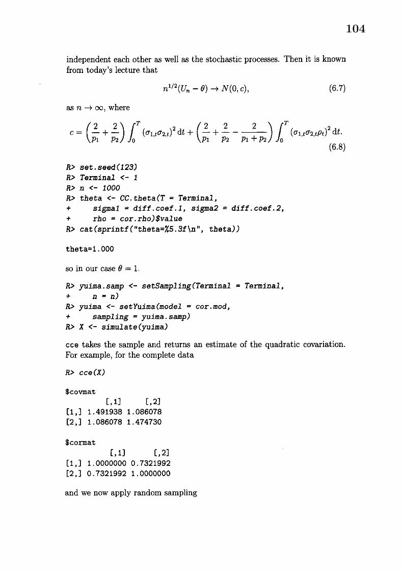
independent each other as well as the stochastic processes. Then it is knownfrom today’s lecture that

$n^{1/2}(U_{n}-\theta)arrow N(0, c)$ , (6.7)

as $narrow\infty$ , where

$c=( \frac{2}{p_{1}}+\frac{2}{p_{2}})\int_{0}^{T}(\sigma_{1,t}\sigma_{2,t})^{2}dt+(\frac{2}{p_{1}}+\frac{2}{p_{2}}-\frac{2}{p_{1}+p_{2}}I\int_{0}^{T}(\sigma_{1,t}\sigma_{2,t}\rho_{t})^{2}dt$ .(6.8)

$R>set.$ seed (123)$R>$ Termin$al<-1$$R>n<-1000$$R>theta<-CC$ . theta $(T=$ Terminal,$+$ sigmal $=$ di$ff$ . coef. 1, sigma2 $=$ di $ff$ . coef. 2,$+$ $rho=$ cor. rho)$va1 $ue$

$R>$ cat (sprintf $(^{ll}$ theta$=/5.3f\backslash n^{tt}$ , theta))

theta$=1.000$

so in our case $\theta=1$ .

$R>yuima.samp<-s$etSampling(Terminal $=$ Terminal,$+$ $n=n)$$R>$ yuima $<$-setYuima (model $=c$or. mod,$+$ $s$ampl $ing=$ yuima. $samp$)

$R>\chi<$-simulate (yuima)

cce takes the sample and returns an estimate of the quadratic covariation.For example, for the complete data

$R>cce(X)$

$covmat[, 1] [, 2]

[1, ] 1.4919381.086078[2,] 1.0860781.474730

$cormat[, 1] [, 2]

[1, ] 1.0000000 0.7321992[2, ] 0.73219921.0000000

and we now apply random sampling

104

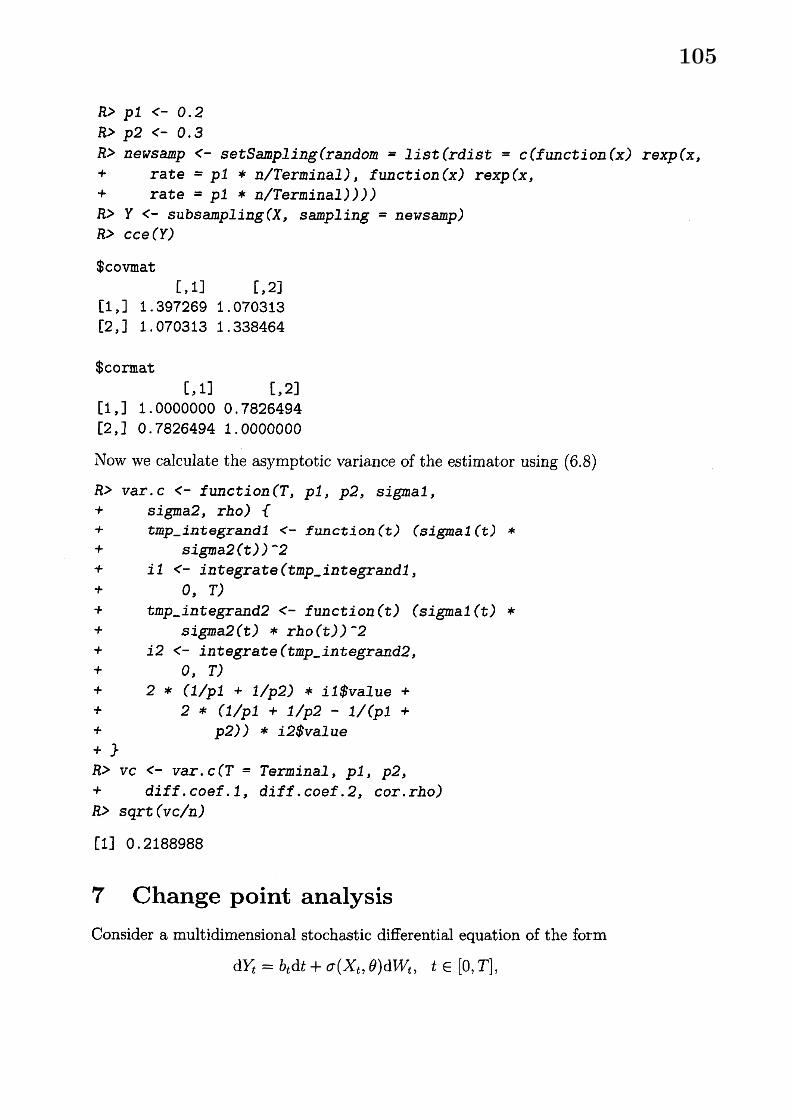
$R>p1<-0.2$$R>p2<-0.3$$R>$ newsamp $<$-setSampling(random $=list$ (rdist $=c(f$unction $(x)$ rexp $(x$ ,$+$ rate $=p1$ $*$ n/Terminal), $f$unction $(x)$ rexp $(x$ ,$+$ rate $=pl$ $*$ n/Terminal) $)))$

$R>Y<$-subsampli$ng$ ($X$ , sampling $=$ news$aIDp$)

$R>cce(Y)$

$covmat[, 1] [, 2]

[1, ] 1.3972691.070313[2, ] 1.0703131.338464

$cormat[, 1] [, 2]

[1, ] 1.0000000 0.7826494[2,] 0.78264941.0000000

Now we calculate the asymptotic variance of the estimator using (6.8)

$R>var$ . $c<$-function(T, $p1,$ $p2$ , signal,$+$ $si$gma2, $rho$ ) {$+$ $tmp_{-}integrand1<$-function $(t)$ (sign$al(t)*$$+$ $si$gma2 $(t))^{\sim}2$

$+$ il $<$-integra$te(tmp_{-}$ integrandl,$+$ $0,$ $T)$

$+$ $tmp_{-}int$egrand2 $<-f$unction (t) (sigmal (t) $*$

$+$ sigma2 (t) $*rho(t))^{\sim}2$

$+$ $i2<$-integrate $(tmp_{-}int$egrand2,$+$ $0,$ $T)$

$+$ 2 $*(1/pI+1/p2)*i$ l$value $+$

$+$ 2 $*(1/p1+1/p2-1/(pl+$$+$ $p2))$ $*$ i2$va$lue$

$+\}$

$R>vc<-var$ . $c(T=$ Terminal, $pl,$ $p2$ ,$+$ $diff$ . coef. 1, $diff$ . coe$f.2,$ $cor.rho$)$R>$ sqrt $(vc/n)$

[I] $0$ . 2188988

7 Change point analysisConsider a multidimensional stochastic differential equation of the form

$dY_{t}=b_{t}dt+\sigma(X_{t}, \theta)dW_{t}$ , $t\in[0, T]$ ,

105

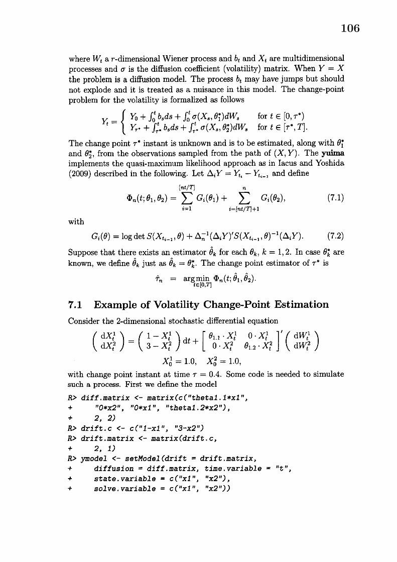
where $W_{t}$ a r-dimensional Wiener process and $b_{t}$ and $X_{t}$ are multidimensionalprocesses and $\sigma$ is the diffusion coefficient (volatility) matrix. When $Y=X$the problem is a diffusion model. The process $b_{t}$ may have jumps but shouldnot explode and it is treated as a nuisance in this model. The change-pointproblem for the volatility is formalized as follows

$Y_{t}=\{\begin{array}{ll}Y_{0}+\int_{0}^{t}b_{s}ds+\int_{0}^{t}\sigma(X_{\epsilon}, \theta_{1}^{*})dW_{s} for t\in[0, \tau^{*})Y_{\tau}\cdot+\int_{\tau}^{t}. b_{s}ds+\int_{\tau}^{t}. \sigma(X_{s}, \theta_{2}^{*})dW_{s} for t\in[\tau^{*}, T].\end{array}$

The change point $\tau^{*}$ instant is unknown and is to be estimated, along with $\theta_{1}^{*}$

and $\theta_{2}^{*}$ , from the observations sampled from the path of (X, Y). The yuimaimplements the quasi-maximum likelihood approach as in Iacus and Yoshida(2009) described in the following. Let $\Delta_{i}Y=Y_{t_{i}}-Y_{t_{i-1}}$ and define

$\Phi_{n}(t;\theta_{1}, \theta_{2})=\sum_{i=1}^{[nt/T]}G_{i}(\theta_{1})+\sum_{i=[nt/T|+1}^{n}G_{i}(\theta_{2})$ , (7.1)

with$G_{i}(\theta)=$ log det $S(X_{t_{i-1}}, \theta)+\triangle_{n}^{-1}(\Delta_{i}Y)’S(X_{t_{i-1}}, \theta)^{-1}(\Delta_{i}Y)$ . (7.2)

Suppose that there exists an estimator $\hat{\theta}_{k}$ for each $\theta_{k},$ $k=1,2$ . In case $\theta_{k}^{*}$ areknown, we define $\hat{\theta}_{k}$ just as $\hat{\theta}_{k}=\theta_{k}^{*}$ . The change point estimator of $\tau^{*}$ is

$\hat{\tau}_{n}$ $=$ $\arg\min_{t\in[0,T]}\Phi_{n}(t;\hat{\theta}_{1},\hat{\theta}_{2})$ .

7.1 Example of Volatility Change-Point EstimationConsider the 2-dimensional stochastic differential equation

$(dX_{t}^{2}dX_{t}^{1})=(\begin{array}{ll}1- X_{t}^{1}3- X_{t}^{2}\end{array})dt+[\theta_{1.1,0\cdot X_{t}^{2}}X_{t}^{1}$ $\theta_{12}\cdot X_{t}^{2}0.\cdot X_{t}^{1}]’(dW_{t}^{2}dW_{t}^{1})$

$X_{0}^{1}=1.0$ , $X_{0}^{2}=1.0$ ,

with change point instant at time $\tau=0.4$ . Some code is needed to simulatesuch a process. First we define the model

$R>diff$ . matrix $<$-matri$x(c$ (“thetal. $1*x1$ “,$+$ $0*x2^{\iota\prime}$ , $\iota\prime o*xl^{ll}$ , thetaI. $2*x2^{\prime\iota}$),$+$ 2, 2)$R>$ drift. $c<-c$ $(” 1-xl ”, 13-x2”)$$R>drift$ . matrix $<$-matrix (dri$ft$ . $c$ ,$+$ 2, 1)$R>$ ymodel $<$-setModel (dri$ft=$ dri $ft$ . matrix,$+$ $dif$fus$ion=diff$ . matrix, $time$ . var$iable=$ “ $t”$ ,$+$ state. variable $=c$ $(”x1$ ”, $\prime\prime x2$ “ $)$ ,$+$ $so1ve$ . variabl $e=c$ $(^{l\prime}x1$ “, $\prime\prime x2’’))$

106

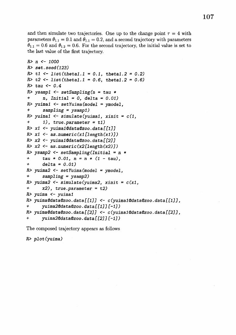
and then simulate two trajectories. One up to the change point $\tau=4$ withparameters $\theta_{1.1}=0.1$ and $\theta_{1.1}=0.2$ , and a second trajectory with parameters$\theta_{1.1}=0.6$ and $\theta_{1.2}=0.6$ . For the second trajectory, the initial value is set tothe last value of the first trajectory.

$R>n<-1000$$R>$ set. seed (123)

$R>t1<$-list (thetal.1 $=0.1$ , thetal. $2=0.2$)

$R>t2<$-list (thetal. 1 $=0.6$ , thetal.2 $=0.6$)

$R>tau<-0.4$$R>ysamp1<$-setSampling(n $=$ tau $*$

$+$ $n$ , Initial $=0,$ $del$ ta $=0.01$ )$R>$ yuimal $<$-setYuima $(mod el=$ ymodel,$+$ $s$ ampl$ing=$ ysamp1)$R>$ yuimal $<$-simulate (yuimal, xini $t=c(1$ ,$+$ 1 $)$ , $true$ . paramet$er=t1$ )

$R>xl<$-yuimal@data@zoo.data $f$flJl$R>xl<-as$ . numeri $c(x1Ll$ength $(x1)])$$R>$ x2 $<$-yuimal@data(Oz$oo$ . data $ff2JJ$

$R>x2<-$ as. numeri $c$ $(x2flength (x2)J)$$R>ysamp2<-setSarpling$ (In$itial=n*$$+$ tau $*0.01,$ $n=n*(1-tau)$ ,$+$ del ta $=0.01)$$R>$ yuima2 $<$-setYuima (model $=$ ymodel,$+$ $s$ ampl $ing=ys$amp2)$R>$ yuima2 $<$-simulate (yuim$a2$ , xini $t=c(xl$ ,$+$ $x2)$ , true. parameter $=t2$)

$R>yuima<$-yuimal$R>$ yuima@data@zoo. data ttlJ] $<-c$ (yuimal@data@zoo. data ttlIJ,$+$ yuima2@data@zoo.data $ff1JJf-1$] $)$

$R>$ yuima@data$($!$)$zoo. data $ff2JJ<-c$ (yuimal@data@zoo. data $ff2JJ$ ,$+$ yuima2@data@zoo.data $ff2JJ$ t-IJ)

The composed trajectory appears as follows

$R>plot$ (yuima)

107

$0$ 2 4 6 8 $\dagger 0$

$t$

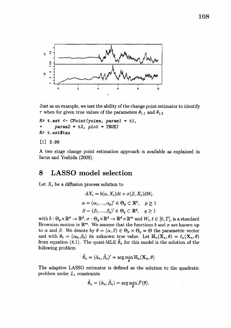
Just as an example, we test the ability of the change point estimator to identify$\tau$ when for given true values of the parameters $\theta_{1.1}$ and $\theta_{1.2}$

$R>t$ . est $<$-CPoint (yu$ima$ , param1 $=t1$ ,$+$ param2 $=t2,$ $plot=$ TRUE)

$R>t$ . est$tau[1] 3. 99

A two stage change point estimation approach is available as explained inIacus and Yoshida (2009).

8 LASSO model selectionLet $X_{t}$ be a diffusion process solution to

$dX_{t}=b(\alpha, X_{t})dt+\sigma(\beta, X_{t})dW_{t}$

$\alpha=(\alpha_{1}, \ldots, \alpha_{p})’\in\Theta_{p}\subset \mathbb{R}^{p}$ , $p\geq 1$

$\beta=(\beta_{1}, \ldots, \beta_{q})’\in\Theta_{q}\subset \mathbb{R}^{q}$, $q\geq 1$

with $b:\Theta_{p}\cross \mathbb{R}^{d}arrow \mathbb{R}^{d},$ $\sigma$ : $\Theta_{q}\cross \mathbb{R}^{d}arrow \mathbb{R}^{d}\cross \mathbb{R}^{m}$ and $W_{t},$ $t\in[0, T]$ , is a standardBrownian motion in $\mathbb{R}^{m}$ . We assume that the functions $b$ and $\sigma$ are known upto $\alpha$ and $\beta$ . We denote by $\theta=(\alpha, \beta)\in\Theta_{p}\cross\Theta_{q}=\Theta$ the parametric vectorand with $\theta_{0}=(\alpha_{0}, \beta_{0})$ its unknown true value. Let $\mathbb{H}_{n}(X_{n}, \theta)=\ell_{n}(X_{n}, \theta)$

from equation (4.1). The quasi-MLE $\tilde{\theta}_{n}$ for this model is the solution of thefollowing problem

$\tilde{\theta}_{n}=(\tilde{\alpha}_{n},\tilde{\beta}_{n})’=\arg\min_{\theta}\mathbb{H}_{n}(X_{n}, \theta)$

The adaptive LASSO estimator is defined as the solution to the quadraticproblem under $L_{1}$ constraints

$\hat{\theta}_{n}=(\hat{\alpha}_{n},\hat{\beta}_{n})=\arg\min_{\theta}\mathcal{F}(\theta)$ .

108

with

$\mathcal{F}(\theta)=(\theta-\tilde{\theta}_{n})\ddot{\mathbb{H}}_{n}(X_{n},\tilde{\theta}_{n})(\theta-\overline{\theta}_{n})’+\sum_{j=1}^{p}\lambda_{n,j}|\alpha_{j}|+\sum_{k=1}^{q}\gamma_{n,k}|\beta_{k}|$

For more details see De Gregorio and Iacus (2010). The tuning parametersshould be chosen as in Zou (2006) in the following way

$\lambda_{n,j}=\lambda_{0}|\tilde{\alpha}_{n,j}|^{-\delta_{1}}$ , $\gamma_{n,k}=\gamma_{0}|\tilde{\beta}_{n,j}|^{-\delta_{2}}$ (8.1)

where $\tilde{\alpha}_{n,j}$ and $\tilde{\beta}_{n,k}$ are the unpenalized QML estimator of $\alpha_{j}$ and $\beta_{k}$ respec-tively, $\delta_{1},$ $\delta_{2}>0$ and usually taken unitary.

8.1 An example of useThe lasso method is implemented in the yuima package. Let us consider thefull CKLS model

$dX_{t}=(\alpha+\beta X_{t})dt+\sigma X_{t}^{\gamma}dW_{t}$

and let us try to estimate the parameter on the U.S. Interest Rates monthlydata from 06/1964 to 12/1989. We prepare the data, the model and theconstraints for optimization

$R>$ library (Ecdat)$R>$ data (Irates)

$R>ra$tes $<$-Irates $f$ , ltrl “]

$R>plot$ (rates)

$R>X<$-window(rates, start $=1964.471$ ,$+$ en$d=1989.333)$$R>mod$ $<$-setModel $(drift=$ “alph$a+beta*x^{lt}$ ,$+$ $di$ffusion $=$ matri $X(”Si_{\mathscr{X}^{a*x^{\sim}gawwa^{\prime l}}}$ ,$+$ 1, 1) $)$

$R>$ yuima $<$-setYuima (data $=setData(X)$ ,$+$ model $=mod$)$R>$ lambda10 $<$-list (alpha $=10$ , beta $=10$ ,$+$ sigma $=10$ , gamma $=10$)

$R>st$art $<$-list (alpha $=1$ , $beta=-0.1$ ,$+$ $si$gma $=0.1$ , gamma $=I$ )

$R>low$ $<$-list (alph$a=-5$ , $beta=-5$ ,$+$ $si$gma $=-5$ , ganmna $=-5$)

$R>upp<$-list (alpha $=8$ , $beta=8_{s}$$+$ $si$gm$a=8$ , gamma $=8$)

and now we apply the lasso function

109

$R>1$assolO $<$-lasso (yuima, 1ambdalO,$+$ $start=st$ar$t,$ $lo$wer $=low,$$+$ $upp$er $=upp$ , method $=|\prime L-BFGS-B$ “ $)$

From which we see that, instead of the general model

$dX_{t}=(\alpha+\beta X_{t})dt+\sigma X_{t}^{\gamma}dW_{t}$

$R>ro$un$d$ ($1$assolO$ml $e$ , 2)

sigma gamma alpha beta0.13 1.44 2.08 $-0.26$

$R>$ round (1assolO$lasso, 2)

sigma gamma alpha beta0.12 1.50 0.59 0.00

the LASSO method selects the reduced model

$dX_{t}=0.6dt+0.12X_{t}^{\frac{3}{2}}dW_{t}$

AcknowledgementsThe author thanks all the members of the Yuima Project Team. All the errorsin this paper are solely of the present author.

ReferencesChambers, J. M. (1998). Programming with Data: A Guide to the S Language.

Springer-Verlag, New York.

De Gregorio, A. and Iacus, S. M. (2010). Adaptive lasso-type estimationfor ergodic diffusion processes. http: //services. bepress. $com/unimi/$statistics/art50/.

Hayashi, T. and Yoshida, N. (2005). On covariance estimation of non-synchronously observed diffusion processes. Bemoulli 11, 359-379.

Hayashi, T. and Yoshida, N. (2006). Nonsynchronous covariance estimatorand limit theorem. Institute of Statistical Mathematics Research Mem-orandum No.1020, 1-40.

Hayashi, T. and Yoshida, N. (2008a). Asymptotic normality of a covarianceestimator for nonsynchronously observed diffusion processes. Annals of theInstitute of Statistical Mathematics 60, 367-406.

110

Hayashi, T. and Yoshida, N. (2008b). Nonsynchronous covariance estima-tor and limit theorem ii. Institute of Statistical Mathematics ResearchMemorandum No.1067, 1-40.

Iacus, S. and Yoshida, N. (2009). Estimation for the changepoint of the volatility in .a stochastic differential equation.$http.\cdot//amiv.org/abs/0906.3108$ .

Yoshida, N. (1992). Estimation for diffusion processes from discrete observa,tion. J. Multivar. Anal. 41, 2, 220-242.

Zou, H. (2006). The adaptive lasso and its oracle properties. J. Amer. Stat.Assoc. 101, 476, 1418-1429.

111

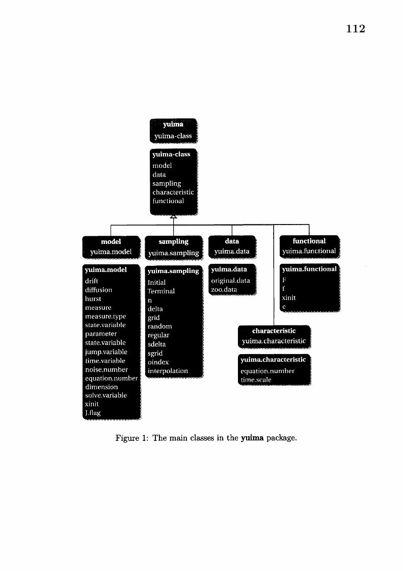
Figure 1: The maln classes in the yuima package.

112