YUEHENG ZHANG - University of Chicago

ON THE PRINCIPAL EIGENVECTOR OF A GRAPH

YUEHENG ZHANG

The University of Chicago

Abstract. The principal ratio of a connected graph G, γ(G), is the ratio

between the largest and smallest coordinates of the principal eigenvector of theadjacency matrix of G. Over all connected graphs on n vertices, γ(G) ranges

from 1 to ncn. Moreover, γ(G) = 1 if and only if G is regular. This indicates

that γ(G) can be viewed as an irregularity measure of G, as first suggestedby Tait and Tobin (El. J. Lin. Alg. 2018). We are interested in how stable

this measure is. In particular, we ask how γ changes when there is a small

modification to a regular graph G. We show that this ratio is polynomiallybounded if we remove an edge belonging to a cycle of bounded length in G,

while the ratio can jump from 1 to exponential if we join a pair of verticesat distance 2. We study the connection between the spectral gap of a regular

graph and the stability of its principal ratio. A naive bound shows that given

a constant multiplicative spectral gap and bounded degree, the ratio remainspolynomially bounded if we add or delete an edge. Using results from matrix

perturbation theory, we show that given an additive spectral gap larger than

2√n, the ratio stays bounded after adding or deleting an edge.

Contents

1. Introduction 22. General preliminaries 3

2.1. Definitions and notation 32.2. Results from linear algebra 42.3. Results from spectral graph theory 6

2.3.1. Observations about the adjacency operator 62.3.2. Existence of the principal eigenvector for a connected graph 62.3.3. Bounds on the largest eigenvalue for a graph 72.3.4. The largest eigenvalue of subgraphs 82.3.5. Graph products 8

3. Preliminary results about the principal eigenvector 93.1. Observations and naive bounds on the ratio 93.2. Chebyshev polynomials and principal eigenvectors 11

3.2.1. Chebyshev polynomials 113.2.2. Applications to prinicpal eigenvectors 11

4. Main results 124.1. Adding or removing an edge in bounded distance 12

4.1.1. Adding an edge 12

Date: Dec 31, 2019.Written for the University of Chicago 2019 Math REU; mentored by Professor Laszlo Babai.

1

ON THE PRINCIPAL EIGENVECTOR OF A GRAPH 2

4.1.2. Removing an edge 144.2. Multiplicative spectral gap and stability of the ratio 154.3. Additive spectral gap and stability of the ratio 16

4.3.1. Existence of graphs with large additive spectral gap andlarge diameter 16

4.3.2. Large additive spectral gap implies bounded ratio 174.4. Open questions 20

Acknowledgments 21References 21

1. Introduction

It is known that the adjacency matrix AG of every connected graph G has asimple largest eigenvalue λ1, and that λ1 has an eigenvector with all-positive coor-dinates, called the principal eigenvector of G, which we denote by q. Therefore aunique-up-to-scaling all-positive eigenvector can be associated with every connectedgraph. Then it is natural to study how q reflects the structure of the graph. Allour discussions will be asympototic as the number of vertices approaches infinityin a family of graph.

Cioaba and Gregory [11] first defined the principal ratio of G, γ(G) = qmax/qmin,to be the ratio between the largest and smallest coordinates of q. This ratio is 1for regular graphs, while it can grow at factorial rate (i.e., γ(G) > ncn for somepositive constant c) [11]. Since γ(G) ≥ 1 where equality holds if and only if G isregular, it is natural to think of γ(G) as a measure of the irregularity of G. Thisview was suggested by Tait and Tobin [13].

A basic observation is that, given a connected graph G with largest eigenvalueλ1 and diameter D, the principal ratio satisfies

(1.1) γ(G) ≤ λD1 .

We are interested in the stability of γ, i.e., how a slight change of G influencesγ(G). In particular, given a d-regular graph G, we ask how γ(G) changes from theconstant 1 if we add or remove one edge in G. (We call the resulting graphs G+ eand G−e, respectively.) We always assume the edge we remove will not disconnectG (i.e., e is a non-bridge edge), so that the principal eigenvector of G−e is defined.

In Section 4.1, we study the cases where the edge we add to or remove from aregular graph is between vertices of bounded distance. We show that

• γ(G + e) can jump to exponential in n when the degree is bounded [The-orem 4.3]. In our example, e connects two vertices at distance 2 in G.By (1.1), boundedness of the degree is necessary here.

• If we remove an edge belonging to a cycle of bounded length in G, γ(G−e)is always polynomially bounded regardless of the degree [Theorem 4.11].

We also study the relevance of the spectral gap to the stability of γ(G) for regulargraphs. In Section 4.2, based on (1.1), we note that

• γ(G± e) is always polynomially bounded in n when G is a bounded-degreeexpander graph, i.e., when the degree is bounded and the spectral gap ofG is bounded from below [Observation 4.15].

YUEHENG ZHANG 3

In Section 4.3.2, we put this problem in the more general context of perturbationsof matrices. By adapting theorems and proofs from Stewart and Sun’s book [5] toour special case, we show that

• If there is an additive spectral gap larger than 2√n, then γ(G±e) is bounded

[Theorem 4.17].

This result does not follow from (1.1). Indeed, in Section 4.3.1 we construct graphswith degree of order n(2+t)/3 and additive spectral gap of order nt, having diam-eter of order n(1−t)/3 for any constant 0 < t < 1. Similar applications of matrixperturbation theory in link analysis for networks can be found in [9].

When computing or giving bounds on the coordinates of the principal eigenvec-tor for certain types of graphs, we take advantage of the properties of Chebyshevpolynomials, a family of orthogonal polynomials which has found numerous appli-cations in discrete mathematics. Here is an incomplete list of the areas of suchapplications:

• the matchings polynomial of graphs, by Heilmann and Lieb [1]• approximate Inclusion–Exclusion, by Linial and Nisan [4]• analysis of Boolean functions, in bounding the real degree of the OR func-

tion, by Nisan and Szegedy [6]• the diameter of regular and bipartite biregular graphs, by van Dam and

Haemers [7]• counting restricted permutations, by Mansour and Vainshtein [8]• the mixing rate of non-backtracking random walks, by Alon et al. [10].

In Section 3.2, we state some properties of Chebyshev polynomials and showtheir connection with the principal eigenvectors of certain graphs.

2. General preliminaries

2.1. Definitions and notation.By a graph we mean what is often called a simple graph (undirected graph with

no self-loops and no parallel edges). G will always denote a connected graph withn vertices. We denote by V (G) and E(G) the set of vertices and edges of G,respectively. We usually identify the set of vertices with the set [n] = 1, 2, . . . , n,so the vertices are labeled 1, . . . , n. We write i ∼G j if vertices i, j are adjacent inG. We denote by NG(j) the set of neighbors of j in G. We use degG(j) to denotethe degree of vertex j in G. We write G for the complement of G. Let distG(i, j)denote the distance between vertices i and j in G. Let D(G) := maxi,j dist(i, j)denote the diameter of G.

We use Mn(R) to denote the set of n×n real matrices. We write j for the all onesvector, and J for the all-ones matrix. We use AG to denote the adjacency matrixof G. We note that AG is a real symmetric matrix, so its eigenvalues are real. Wewrite λ1(G) ≥ λ2(G) ≥ · · · ≥ λn(G) to denote the eigenvalues of AG. We alsodenote λ1(G) by λG. We write q(G) for the principal eigenvector of AG scaled tohave l2 norm 1. Let qi(G) denote the coordinate corresponding to vertex i in q(G).We write qmax(G) and qmin(G) for the maximum and minimum coordinates of q(G),and vmax(G) and vmin(G) for corresponding vertices. Recall that the principal ratioof G is defined as

(2.1) γ(G) :=qmax(G)

qmin(G).


We write LG for the Laplacian of G, defined as the n× n matrix

LG = diag(deg(1),deg(2), . . . ,deg(n))−AG.LG is positive semidefinite. The principal eigenvalue of LG is defined to be theeigenvalue corresponding to the eigenvector j; its value is zero. We write δ(G) todenote the smallest non-principal eigenvalue of LG. We note that δ(G) = 0 if andonly if G is disconnected. δ(G) is the algebraic connectivity of the graph G, as firstdefined by Fiedler [2].

For a d-regular graph G, let fA(t) be the characteristic polynomial of its adja-cency matrix AG. The characteristic polynomial of the Laplacian LG is

(2.2) fL(t) = fA(d− t).It follows that

(2.3) δ(G) = d− λ2(G).

We refer to the right-hand side as the additive spectral gap of G. We refer to

(2.4)δ(G)

d= 1− λ2

das the multiplicative spectral gap of G. We use this terminology for regular graphsonly.

In all notation, we omit the graph G when it is clear from context.Let Cn denote the cycle with n vertices. Let Pr denote the path with r vertices;

it has r − 1 edges. Let Ks denote the clique with s vertices; it has(s2

)edges.

Following the notation used in previous papers on this subject, we use Pr ·Ks todenote the graph obtained by merging the vertex at one end of Pr with one vertexin Ks. So Pr ·Ks has n = r+ s−1 vertices, r−1 +

(s2

)edges, and diameter r. This

has been called a kite graph or a lollipop graph. We will call it a kite graph.By a family of graphs, we mean an infinite set of non-isomorphic finite graphs.Let f(n) ≥ 1. We say the rate of growth of f(n) is polynomially bounded if for all

sufficiently large n, f(n) < nc for some constant c. We say f(n) is exponential if forall sufficiently large n, f(n) ≥ an for some constant a > 1. We say f(n) has factorialgrowth if for all sufficiently large n, f(n) ≥ ncn for some positive constant c.

Given a family G of graphs, we label the graphs as G1, . . . , Gi, . . . , and letn1, . . . , ni, . . . be the corresponding number of vertices. We say γ(G) is polyno-mially bounded in n if there is some constant c such that for all sufficiently large i,γ(Gi) < nci . We say γ(G) grows exponentially in n if there is some constant a > 1such that for all sufficiently large i, Gi > ani .

2.2. Results from linear algebra.In this section we introduce results from linear algebra that we will use for later

proofs. Orthonormality in Rn refers to the standard dot product. Given a matrix A,we write aij for the entry on the i-th row and in the j-th column of A, and we writeA = (aij).

Definition 2.5. For an m × n real matrix M , the operator norm induced by l2

vector norm (‖ · ‖) is

‖M‖ = supx∈Rn, x6=0

‖Mx‖‖x‖

.

Fact 2.6. In addition to being subadditive, the operator norm is also submulti-plicative, i.e., ‖AB‖ ≤ ‖A‖‖B‖ for A,B ∈Mn(R).

YUEHENG ZHANG 5

Fact 2.7. For a symmetric real matrix M , ‖M‖ = max1≤i≤n |λi|. Moreover, if Mis non-negative, max1≤i≤n |λi| is attained by λ1. In particular, for the adjacencymatrix AG of a graph G,

(2.8) ‖AG‖ = λ1(G).

Theorem 2.9 (Spectral theorem for real symmetric matrices). If M is an n × nreal symmetric matrix (i.e., M = MT ), then M has an orthonormal eigenbasisover R. In particular, all eigenvalues of M are real.

Definition 2.10 (Fractional powers of positive semidefinite real symmetric matri-ces). Let M ∈ Mn(R) be symmetric and positive semidefinite. Then we can writeM as M = QΛQT where Q is an orthogonal matrix, Λ = diag(λ1, . . . , λn), andλi ≥ 0. For a ∈ R, we define

Ma := Qdiag(λa1 , . . . , λan)QT .

This definition is sound. (It does not depend on the particular choice of Q.) Itfollows that for a, b ∈ R, Ma ·M b = Ma+b.

In the rest of Section 2.2, A = (aij) will always denote a real symmetric n × nmatrix with eigenvalues λ1 ≥ λ2 ≥ · · · ≥ λn.

Definition 2.11. A multiset is a set in which elements are allowed to have multipleinstances. We denote a multiset by double braces. For example, a, a, a, b, c, cis a multiset. We also write a, a, a, b, c, c as a3, b, c2.Definition 2.12. The spectrum of an n× n matrix M is the multiset of its eigen-values. We denote it by spec(M).

Fact 2.13 (Spectrum of polynomials of a matrix). If g is a polynomial, then

spec(g(A)) = g(λ1), g(λ2), . . . , g(λn).Definition 2.14. The Rayleigh quotient of the matrix A is the function

RA(y) =yTAy

yTy=

∑1≤i,j≤n aijyiyj∑n

i=1 y2i

,

defined for y ∈ Rn, y 6= 0.

Observation 2.15. If y is an eigenvector to eigenvalue λi, then RA(y) = λi.

Theorem 2.16 (Rayleigh’s principle).

λ1 = maxy

RA(y).

λn = maxy

RA(y).

Moreover, RA(y) = λ1 if and only if y is an eigenvector to λ1.

Corollary 2.17. Given vector y = (y1, . . . , yn)T , we let |y| be the vector (|y1|, . . . , |yn|)T .If y is an eigenvector to eigenvalue λ1, then |y| is also an eigenvector to λ1.

Definition 2.18. Let B = (bij) be an m× n matrix and let M be a p× q matrix.The Kronecker product of B and M , B ⊗M , is the mp× nq matrix

b11M b12M · · · b1nMb21M b22M · · · b2nM

......

......

bm1M bm2M · · · bmnM

.


Fact 2.19. Let B ∈ Mn(R) and M ∈ Mm(R). Let the eigenvalues of B beλ1 ≥ · · · ≥ λn and let the eigenvalues of M be µ1 ≥ · · · ≥ µm. Then

spec(B ⊗M) = λiµj , 1 ≤ i ≤ n, 1 ≤ j ≤ m.

2.3. Results from spectral graph theory.In this section we introduce well-known results from spectral graph theory that

will be of use later.2.3.1. Observations about the adjacency operator.

In Sections 2.3.1 through 2.3.3, we fix the graph G and write A for AG.We first note how the adjacency operator A of a graph G acts on vectors.

Observation 2.20. Given y = (y1, . . . , yn), the ith coordinate of Ay is given by

(Ay)i =∑j:i∼j

yj .

Corollary 2.21. If y = (y1, . . . , yn) is an eigenvector of A to eigenvalue ρ, then

ρyi =∑j:j∼i

yj .

Recall that j denotes the all-ones vector.

Corollary 2.22. j is an eigenvector of A if and only if G is regular.

Proof. Suppose G is d-regular. Then Aj = (deg(1),deg(2), . . . ,deg(n))T = dj.Suppose Aj = dj. Then for any i ∈ n, |N(i)| = (d · 1)/1 = d.

2.3.2. Existence of the principal eigenvector for a connected graph.In this section we establish the existence of the principal eigenvector for a con-

nected graph. This follows from the Perron–Frobenius theorem for irreducible ma-trices, though given that the adjacency matrix is real and symmetric, it can beproved in much simpler ways using Rayleigh’s principle.

Proposition 2.23. If G is a connected graph and y is an eigenvector to eigenvalueλ1, then y has no zero coordinates.

Proof. It suffices to prove that |y| has no zero entries. By Corollary 2.17, |y|is an eigenvector to eigenvalue λ1. Suppose |yi| = 0. Then by Corollary 2.21,∑j:j∼i |yj | = 0. Therefore |yj | = 0 for all j ∼ i. Since G is connected, by repeating

this argument we have y = 0, but by assumption y 6= 0.

Proposition 2.24. If G is a connected graph and y is an eigenvector to eigenvalueλ1, then the coordinates of y are either all positive or all negative.

Proof. Suppose there are entries of opposite signs in y. Since G is connected andy has no zero entries, there has to be edges between vertices of positive entry andvertices of negative entry. Since the entries of AG corresponding to these edgesare 1, we can strictly increase RAG

(y) by changing the sign of all negative entriesinto positive. But this contradicts Theorem 2.16 (Rayleigh’s principle).

Corollary 2.25. For a connected graph G, λ1 is simple.

Proof. Two all-positive or all-negative vectors cannot be orthogonal.

Theorem 2.26. For every connected graph G, the largest eigenvalue λ1 is simple,and it has a unique-up-to-scaling all-positive eigenvector (the principal eigenvector).

YUEHENG ZHANG 7

Proof. Proposition 2.24 together with Corollary 2.17 proves the existence of anall-positive eigenvector to λ1. Since λ1 is simple, this eigenvector is unique up toscaling.

Corollary 2.27. If G is connected and y is an eigenvector to eigenvalue λ withall-positive coordinates, then λ is the largest eigenvalue of A.

Proof. Since λ1 is simple, any eigenvector y to an eigenvalue other than λ1 mustbe orthogonal to the principal eigenvector.

Corollary 2.28. For a connected d-regular graph G, λ1 = d.

Proof. Follows from Corollary 2.22.

Corollary 2.29. For the clique on n vertices, λ1 = n− 1.

Observation 2.30. Corollary 2.28 also proves (2.3).

2.3.3. Bounds on the largest eigenvalue for a graph.Let ∆ denote max1≤i≤n deg(i), the maximum degree of G.

Fact 2.31. For every graph G, λ1 ≤ ∆. For connected graphs, equality holds ifand only if G is regular.

Proof. Let y be an eigenvector to λ1, and let yi be the maximum coordinate, then

λ1yi =∑j:i∼j

yj ≤ ∆yi.

Therefore λ1 ≤ ∆. Suppose G is d-regular, then ∆ = d = λ1 by Corollary 2.28.On the other hand, suppose G is connected and λ1 = ∆. Then ∆yi =

∑j:i∼j yj .

Therefore vertex i has degree ∆ and the neighbors of i have coordinates as largeas i. Repeat this argument for the neighbors of i. Since the graph is connected, wehave that every vertex has degree ∆ and the same coordinate as yi.

We denote the arithmetic and quadratic mean of the degrees of vertices by

(2.32) davg :=

∑ni=1 deg(i)

n

and

(2.33) dqavg :=

√∑ni=1 deg(i)2

n.

It is well-known that the quadratic mean of a multiset of numbers is not less thanthe arithmetic mean.

Fact 2.34. For every graph G, λ1 ≥ davg.

Proof. By Theorem 2.16 (Rayleigh’s principle),

λ1(A) = maxy 6=0

RA(y) ≥ RA(j) =jTAj

jT j=

∑ni=1 deg(i)

n.

We can improve this to a stonger bound.

Fact 2.35. For every G, λ1 ≥ dqavg.


Proof. Let spec(G) = λ1, . . . , λn, where λ1 ≥ · · · ≥ λn. By Fact 2.13,

spec(A2) = λ21, . . . , λ2n.

Let y = (y1, . . . , yn)T be an eigenvector of λn, then by Observation 2.15,yTGy

yTy= λn.

Since A is non-negative,

|y|TA|y||y|T |y|

=

∑ni=1

∑nj=1 |yi|aij |yj |yTy

≥|∑ni=1

∑nj=1 yiaijyj |

yTy=∣∣∣yTAy

yTy

∣∣∣ = |λn|.

Then by Theorem 2.16 (Rayleigh’s principle), λ1 ≥ |λn|. Therefore λ21 is the largesteigenvalue of A2. Again by Rayleigh’s principle,

λ21 ≥jTA2j

jT j=

jTATAj

jT j=

(Aj)TAj

jT j=

∑ni=1 deg(i)2

n.

Thus

λ1 ≥√∑n

i=1 deg(i)2

n.

2.3.4. The largest eigenvalue of subgraphs.

Fact 2.36. If H is a proper subgraph of a connected graph G, then λ1(G) > λ1(H).

Proof. Let y be a non-negative eigenvector of AH to eigenvalue λ1(H), which existsby Corollary 2.17. Let G have n vertices. We define y as the vector with ncoordinates obtained by adding zero coordinates to y where vertices are deleted. Ify has zero coordinates, then by Proposition 2.23, y is not an eigenvector to λ1(G).Therefore by Rayleigh’s principle, λ1(G) > RAG

(y) ≥ RAH(y) = λ1(H). If y does

not have zero coordinates, then y = y. For H to be a proper subgraph of G, atleast one edge is deleted. Therefore

λ1(G) ≥ yTAGy

yT y=

yTAGy

yTy>

yTAHy

yTy= λ1(H).

2.3.5. Graph products.

Notation 2.37. Given a graph G and U ⊆ V (G), we denote the induced subgraphof G on the set U by G[U ].

Definition 2.38. For graphs H = (W,F ) and G = (V,E), the Cartesian productof H and G, denoted by HG, is the graph with the set W × V as vertices, and(w1, v1) ∼ (w2, v2) if and only if w1 = w2 and v1 ∼G v2, or v1 = v2 and w1 ∼H w2.For each v ∈ V , we call (HG)[W × v] the horizontal layer corresponding to v.For each w ∈ W , we call (HG)[w × V ] the vertical layer corresponding to w.The horizontal layers are copies of H and the vertical layers are copies of G.

Definition 2.39. For graphs H = (W,F ) and G = (V,E), the lexicographic productof H and G, denoted by H G, is the graph with the set W × V as vertices, and(w1, v1) ∼ (w2, v2) if and only if either w1 ∼H w2 or w1 = w2 and v1 ∼G v2. Foreach w ∈W we call (H G)[w × V ) the vertical layer corresponding to w.

Recall that J denotes the all-ones matrix.

Observation 2.40. The ajacency matrix of G H is AG⊗ J|V (H)|+ I|V (G)|⊗AH .

YUEHENG ZHANG 9

3. Preliminary results about the principal eigenvector

As previously introduced, G will always denote a connected graph. We writeλ for λ1, the largest eigenvalue of the adjacency matrix of G. We use q to meanthe principal eigenvector of the adjacency matrix, the all-positive eigenvector to λ1.We assume q is scaled to have l2 norm 1 unless otherwise stated.

3.1. Observations and naive bounds on the ratio.First, we note that q reflects the symmetries of G.

Notation 3.1. Given a permutation π on a set X and an element a ∈ X, we writeπ(a) for the image of a under π. We use Mπ to mean the row permutation matrixof π, where Mπ

i,j = 1 if π(j) = i and Mπi,j = 0 otherwise. Given a vector y, we write

π(y) to denote Mπy.

Definition 3.2. Given a permutation group S on a set X, the orbit of a ∈ Xunder S is

OS(a) := π(a) | π ∈ S.

Definition 3.3. Given a graph G, an automorphism of G is a permutation π onthe set of vertices that preserves adjacency relation, i.e., for each pair of verticesi, j ∈ V (G), π(i) ∼ π(j) if and only if i ∼ j.

Notation 3.4. We note that the set of automorphisms of a graph G is a groupunder composition. We denote this group by Aut(G). For a vertex i ∈ V (G), wedenote the orbit of i under Aut(G) by O(i).

Observation 3.5. If π is an automorphism of G, then AG = MπAG(Mπ)T .

Proposition 3.6. Given a graph G and π ∈ Aut(G), if y is an eigenvector of AGto eigenvalue ρ, then π(y) is also an eigenvector of AG to ρ.

Proof. Since any permutation matrix is an orthonormal matrix, (Mπ)TMπ = I.Then by Observation 3.5, AGM

π = MπAG. Then AGMπy = MπAGy = ρMπy.

Therefore π(y) is an eigenvector of AG to ρ.

Fact 3.7. The principal eigenvector q is constant on orbits of Aut(G), i.e., ifj ∈ O(i), then qi = qj .

Proof. Let j ∈ O(i). Then there is π ∈ Aut(G) with π(i) = j. By Proposition 3.6,π(q) is an eigenvector to λ. Since q is all-positive, π(q) is also all-positive. Thereforeby Theorem 2.26, π(q) = q when scaled to the same norm. Therefore qi = qj .

Next we note some basic bounds on the ratio between the coordinates of q.

Observation 3.8. For two vertices i, j in G, let dist(i, j) = k. Then

qjqi≤ λk.

Proof. If dist(i, j) = 0, then qj/qi = 1 = λ0. If dist(i, j) = 1, then by Corol-lary 2.21, λqi =

∑w:w∼i qw ≥ qj since all qw are positive. Now, suppose k ≥ 2 and

qw/qi ≤ λk−1 for all vertices w at distance k − 1 from i. We know j is adjacent toat least one vertex w at distance k − 1 from i. Then

qjqi

=qjqw· qwq1≤ λ · λk−1 = λk.


Recall that D denotes the diameter of the graph.

Corollary 3.9. For every connected graph G with diameter D,

γ ≤ λD ≤ ∆D ≤ (n− 1)D.

Corollary 3.10. If D is bounded for some family G of graphs , then γ(G) is poly-nomially bounded in n.

Since D is relevant in bounding the ratio, we introduce a bound on D for regulargraphs.

Fact 3.11. Let G be a connected d-regular graph. Then D ≤ 3n

d.

Proof. Pick v0, vD in G so that dist(v0, vD) = D. Let v0, v1, . . . , vD be a shortestpath from v0 to vD. Any vi, vj with |i− j| ≥ 3 cannot have any common neighbors,since otherwise the path will not be a shortest path. Thus

d

⌈D

3

⌉≤ n.

Therefore D ≤ 3n/d.

We know D(G + e) ≤ D(G) for any e ∈ G. The following result shows thatD(G + e), and consequently, also D(G − e) (if still connected), cannot differ fromDG by more than a factor of 2.

Fact 3.12. For any connected graph G with D(G) = D and e ∈ E(G),

D(G+ e) ≥ 1

2D(G).

Proof.(Notation: By distl(x, y), where l is a path, we mean the distance between x and yalong the path.)We need to prove that there is a pair of vertices at distance at least D

2 in G + e.Let u, v ∈ V (G) be such that distG(u, v) = D. If distG+e(u, v) = D, we are done.Otherwise, let p be a shortest path between u and v in G, and q a shortest pathbetween u and v in G + e. Then e must be on q. Denote by x the endpoint of ewhich is closer to u on q, and by y the other endpoint. Pick the middle vertex wof p with distp(u,w) = dD2 e. If distG+e(u,w) = distG(u,w) = dD2 e, we are done.Otherwise, any shortest path r in G + e from u to w must pass through edge e.Suppose we go along r from u to w, by the optimality of q, we can assume that rand q overlap from u to y. Now we look at the vertex w′ adjacent to w on p whichis closer to u than to v. We have

(3.13) distG(w′, v) = distp(w′, v) =

⌊D

2

⌋+ 1.

We claim that there is a shortest path in G + e from w′ to v that does not passthrough e. Let s be a shortest path in G + e from w′ to v that passes through e.By the optimality of q, we may assume that s and q overlap from x to v. Then bythe optimality of r,

dists(x,w′) + distG+e(w

′, w) ≥ distr(x,w) = distG+e(x, y) + distr(y, w),

that is,dists(x,w

′) ≥ distr(y, w).

YUEHENG ZHANG 11

Therefore

dists(w′, y) = dists(w

′, x) + distG+e(x, y) ≥ distG+e(w′, w) + distr(w, y).

Thus s is equivalent to a path that does not pass through e in G+ e. As a result,a shortest path between w′ and v in G+ e is also available in G. Then by (3.13),

distG+e(w′, v) = distG(w′, v) =

⌊D

2

⌋+ 1.

3.2. Chebyshev polynomials and principal eigenvectors.

3.2.1. Chebyshev polynomials.

The Chebyshev polynomials of the first kind, Tn, can be characterized by therecurrence

(3.14) Tn+1(t) = 2t · Tn(t)− Tn−1(t),

with initial values T0(t) = 1 and T1(t) = t.The Chebyshev polynomials of the second kind, Un, can be characterized by the

same recurrence

(3.15) Un+1(t) = 2t · Un(t)− Un−1(t),

with initial values U0(t) = 1 and U1(t) = 2t.

Fact 3.16. When |t| ≥ 1, the explicit formula for Tn is

(3.17) Tn(t) =1

2

((t−√t2 − 1

)n+(t+√t2 − 1

)n),

and the explicit formula for Un is

(3.18) Un(t) =

(t+√t2 − 1

)n+1

−(t−√t2 − 1

)n+1

2√t2 − 1

.

Fact 3.19. The roots of Tn are cos

(π(k + 1/2)

n

), k = 0, . . . , n− 1. The roots of

Un are cos

(kπ

n+ 1

), k = 1, . . . , n.

3.2.2. Applications to prinicpal eigenvectors.

Fact 3.20. When x > 1, both Tn(x) and Un(x) are strictly increasing.

Definition 3.21. A pendant path of length k in G consists of k vertices such thatthe induced subgraph on them is a path; moreover, one vertex has degree 1 in Gand k − 2 vertices have degree 2 in G. For example, in the graph Pr ·Ks, there isa pendant path of length r.

Observation 3.22. Let 1, 2, . . . , k be a pendant path in G where consecutive ver-tices are adjacent and deg(1) = 1. Then for 1 ≤ j ≤ k,

qjq1

= Uj−1

(λ

2

).

Proof. By Corollary 2.21, λq1 = q2 and qj+1 = λqj − qj−1 for 1 ≤ j ≤ n − 1.Therefore qj/q1 satisfies the initial values and recurrence relation of Uj−1(λ/2).


Observation 3.22 along with Fact 2.36 can be used to show that most kite graphshave a very large (factorial) principal ratio, since Pr · Ks has a pendant path oflength r and λ is larger than s − 1. In fact, Tait and Tobin [13] proved that themaximum principal ratio over all graphs of n vertices is attained by a kite graph.

4. Main results

Let G be a d-regular graph. As introduced before, we use G + e to denote thegraph obtained by adding an edge e ∈ E(G) to G, and G− e to denote the graphobtained by deleting an edge e ∈ E(G) from G. We always assume G − e is stillconnected. We are interested in the possible asymptotic behaviors of γ(G+ e) andγ(G− e).

We first make two simple observations.

Observation 4.1. If the diameter D(G) is bounded, then γ(G±e) is polynomiallybounded in n.

Proof. Fact 3.12 shows that D(G ± e) is also bounded, and the statement followsfrom Cororllary 3.10.

Observation 4.2. If d is linear in n, then γ(G± e) is polynomially bounded in n.

Proof. Fact 3.11 shows that D(G) is bounded, and the statement follows fromObservation 4.1.

4.1. Adding or removing an edge in bounded distance.

4.1.1. Adding an edge.We show that if we add an edge e between two vertices at distance 2 to a

connected regular graph G of bounded degree, then γ(G+ e) can be exponential.Let e = 1, 2.

Theorem 4.3. For any fixed d, there is a family G of connected d-regular graphswhere for each Gi ∈ G, there is an edge ei ∈ Gi whose endpoints are at distancetwo in Gi − ei, such that for the family

G′ = Gi + ei | Gi ∈ G,γ(G′) grows exponentially in n.

The proof of this theorem will be based on a series of constructions. The graphsproduced by Construction 4.6 and Construction 4.7 are the pair of graphs that areused in the proof.

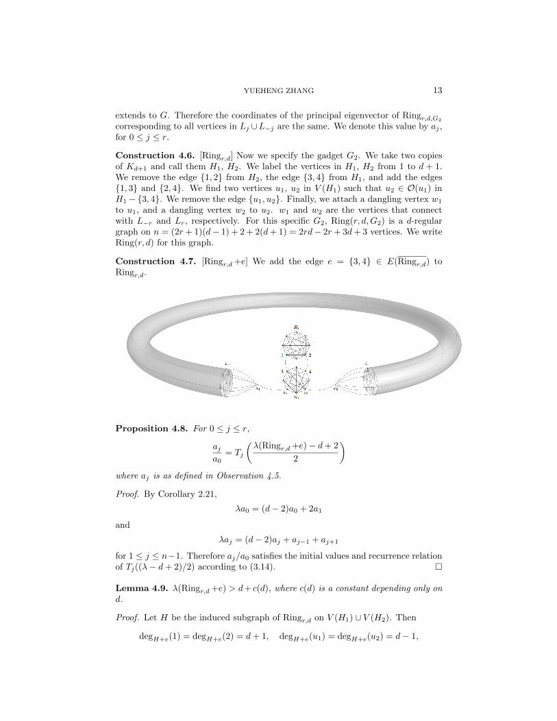
Construction 4.4 (Ringr,d,G2). Let r ≥ 0 be a parameter. We label the vertices

in P2r+1 from one end to the other end as p−r, p−r+1, ..., p−1, p0, p1, ..., pr−1, pr.Let G1 = P2r+1Kd−1. We label the vertical layer corresponding to pi as Li. LetG2, which we will call a “gadget,” be a connected graph with two vertices v1, v2 ofdegree 1 and all other vertices of degree d, and an automorphism that switches v1and v2. We connect v1 with every vertex in L−r and connect v2 with every vertexin Lr. We call the graph obtained Ringr,d,G2

.

Observation 4.5. Let X ≤ Aut(G1) be the subgroup of automorphisms of G1

that fixes the vertical layers and permutes the horizontal layers. The orbits of Xare the vertical layers. X is isomorphic to the symmetric group Sd−1. This groupextends to G. The automorphism of G1 that switches Lj and L−j for 0 ≤ j ≤ r also

YUEHENG ZHANG 13

extends to G. Therefore the coordinates of the principal eigenvector of Ringr,d,G2

corresponding to all vertices in Lj ∪L−j are the same. We denote this value by aj ,for 0 ≤ j ≤ r.

Construction 4.6. [Ringr,d] Now we specify the gadget G2. We take two copiesof Kd+1 and call them H1, H2. We label the vertices in H1, H2 from 1 to d + 1.We remove the edge 1, 2 from H2, the edge 3, 4 from H1, and add the edges1, 3 and 2, 4. We find two vertices u1, u2 in V (H1) such that u2 ∈ O(u1) inH1 −3, 4. We remove the edge u1, u2. Finally, we attach a dangling vertex w1

to u1, and a dangling vertex w2 to u2. w1 and w2 are the vertices that connectwith L−r and Lr, respectively. For this specific G2, Ring(r, d,G2) is a d-regulargraph on n = (2r+ 1)(d− 1) + 2 + 2(d+ 1) = 2rd− 2r+ 3d+ 3 vertices. We writeRing(r, d) for this graph.

Construction 4.7. [Ringr,d +e] We add the edge e = 3, 4 ∈ E(Ringr,d) toRingr,d.

Proposition 4.8. For 0 ≤ j ≤ r,

aja0

= Tj

(λ(Ringr,d +e)− d+ 2

2

)where aj is as defined in Observation 4.5.

Proof. By Corollary 2.21,

λa0 = (d− 2)a0 + 2a1

and

λaj = (d− 2)aj + aj−1 + aj+1

for 1 ≤ j ≤ n−1. Therefore aj/a0 satisfies the initial values and recurrence relationof Tj((λ− d+ 2)/2) according to (3.14).

Lemma 4.9. λ(Ringr,d +e) > d+ c(d), where c(d) is a constant depending only ond.

Proof. Let H be the induced subgraph of Ringr,d on V (H1) ∪ V (H2). Then

degH+e(1) = degH+e(2) = d+ 1, degH+e(u1) = degH+e(u2) = d− 1,


while the rest of the vertices in H + e are of degree d. Then by Fact 2.36 andFact 2.35,

λ(Ringr,d +e) > λ(H + e) ≥ dqavg(H + e) =

√(2d+ 2)d2 + 4

2d+ 2= d

√1 +

2

d2(d+ 1).

Let

c(d) :=2

3d(d+ 1).

Since√

1 + x > 1 +1

3x when 0 < x < 3,

λ(G+ e) > d+ c(d).

Proof of Theorem 4.3. By Lemma 4.9,

λ(Ringr,d +e)− d+ 2

2> 1 +

1

3d(d+ 1).

By Observation 4.8, Fact 3.20, and Fact 3.16,

γ(Ringr,d) ≥ara0

= Tr

(λ(Ringr,d +e)− d+ 2

2

)> Tj(1+

1

3d(d+ 1)) >

1

2

(1 +

1

3d(d+ 1)

)r.

Since r =n− 3d− 3

2d− 2and d is bounded,

γ(Ringr,d) > (a(d)− ε)n

where

a(d) :=

(1 +

1

3d(d+ 1)

)1/(2d−2)

and 0 < ε < a− 1 is any fixed constant.

4.1.2. Removing an edge.We show that in the case of removing an edge e = 1, 2 when distG−e(1, 2) is

bounded, γ(G−e) is polynomially bounded for all D. We make use of the followingtheorem.

Let e = 1, 2.

Theorem 4.10 (Cioaba, Gregory, Nikiforov[12]). If G is a connected nonregulargraph with n vertices, diameter D, and maximum degree ∆, then

∆− λG ≥1

n(D + 1).

Theorem 4.11. For a connected d-regular graph G and an edge e = 1, 2 ∈ E(G),if distG−e(1, 2) < c where c is some constant, then γ(G−e) is polynomially boundedin n.

Lemma 4.12. qmin(G− e) is either q1 or q2.

Proof. If qmin corresponds to some vertex j with degree d, then the average of thecoordinates corresponding to the neighbors of j would be

λ(G− e)qjd

<λ(G− e)qjλ(G− e)

= qj ,

which is a contradiction.

YUEHENG ZHANG 15

Proof of Theorem 4.11. Without loss of generality suppose q1 = qmin. Then sum-ming n equations of the form λ(G− e)qi =

∑j:j∼i qj , we have

λ(G− e)n∑i=1

qi = (d− 1)q1 + (d− 1)q2 + dq3 + · · ·+ dqn = d

(n∑i=1

qi

)− q1 − q2.

Therefore by Theorem 4.10,

q1 + q2∑ni=1 qi

= d− λ(G− e) ≥ 1

n(D(G− e) + 1)≥ 1

n2.

By Observation 3.8, q2 ≤ λ(G− e)cq1. Therefore

γ(G− e) <∑ni=1 qiq1

≤ n2(

1 +q2q1

)≤ n2(1 + λ(G− e)c) < n2(1 + dc).

4.2. Multiplicative spectral gap and stability of the ratio.We use a known bound on the diameter of a graph in terms of the spectral graph

to show that γ(G± e) is polynomially bounded for bounded-degree expanders.

Definition 4.13. For 0 < ε < 1, a regular graph of degree d is an ε-expander ifλ2 ≤ (1− ε)d, i.e., δ ≥ εd.

We note that this definition implies that an expander graph is connected.

Theorem 4.14 (N. Alon, V. D. Milman[3]). Let G be a connected graph on nvertices with maximum degree ∆ and let δ denote the smallest positive eigenvalueof the Laplacian matrix δ. Then

D(G) ≤ 2

⌊√2∆

δlog2 n

⌋.

Corollary 4.15. For expander graphs G with bounded degree, γ(G ± e) is poly-nomially bounded in n. More specifically, for an ε-expander graph G with boundeddegree d,

(4.16) γ(G+ e) ≤ n4√

2/ε log2(d+1).

Proof. By definition,

∆(G)

δ(G)=

d

δ(G)≤ 1

ε.

Then

D(G) ≤ 2

⌊√2

εlog2 n

⌋.

By Fact 3.12,

D(G± e) ≤ 4

⌊√2

εlog2 n

⌋.


Since γ ≤ ∆D (Corollary 3.9),

γ(G± e) ≤ (d+ 1)4⌊√

2/ε log2 n⌋

≤ (d+ 1)4√

2/ε log2 n

= 24√

2/ε log2 n log2(d+1)

= n4√

2/ε log2(d+1).

4.3. Additive spectral gap and stability of the ratio.We show that a large ((2 + ε)

√n) additive spectral gap implies that γ(G± e) is

bounded. Specifically, we prove the following.

Theorem 4.17. Let G be a connected d-regular graph. If the spectral gap δ = d−λ2of G satisfies δ >

2

c

√n+ 2 for some value 0 < c < 1, then

γ(G± e) < 1 + c

1− c.

To motivate this result, we first point out that graphs with such an additivespectral gap are not necessarily expanders. Indeed, when d is larger than Θ(

√n),

the multiplicative spectral gap of graphs with a Θ(√n) additive spectral graph will

go to zero. Moreover, the diameter of graphs with such an additive spectral gapcan still grow quite fast (polynomially in n), approaching the upper bound derivedfrom Theorem 4.14.

4.3.1. Existence of graphs with large additive spectral gap and large diameter.

Proposition 4.18. For a regular graph with additive spectral gap δ, the diameterD is O((n/δ)1/3(log n)2/3).

Proof. Let the regular graph have degree d. From Theorem 4.14, we know that

(4.19) D2 ≤ cdδ

(log n)2

where c is some constant. By Fact 3.11, we also have

(4.20) D ≤ 3n

d.

Multiplying (4.19) and (4.20), we have

(4.21) D ≤ (3c)1/3(nδ

)1/3(log n)2/3.

Corollary 4.22. For a regular graph with an Ω(√n) additive spectral gap, the

diameter is O(n1/6(log n)2/3).

We show that this bound is nearly tight.

Proposition 4.23. There are connected regular graphs with diameter (1/2)n1/6

and an additive spectral gap of cn1/2 where c = 2π2(1 +O(n−1/3)).

We prove a more general statement.

Proposition 4.24. For any constant 0 < t < 1, there are connected regular graphswith diameter (1/2)n(1−t)/3 and an additive spectral gap of cnt wherec = 2π2(1 +O(n(2t−2)/3)).

YUEHENG ZHANG 17

Proof. Recall the lexicographic product and its properties in Definition 2.39, Ob-servation 2.40, and Fact 2.19. Let G := Cr Ks where r · s = n. Then G is aconnected regular graph of degree 2s and diameter br/2c. The adjacency matrix ofG can be expressed as

(4.25) AG = ACr⊗ Js + Ir ⊗ 0 = ACr

⊗ Js.Since

(4.26) spec(Js) = s, 0s−1,we have

(4.27) spec(G) = sλ1(Cr), sλ2(Cr), . . . , sλr(Cr), 0(s−1)r.

Thusδ(G) = s(λ1(Cr)− λ2(Cr)).

It is well-known that the eigenvalues of a cycle Cr are 2 cos

(2πj

r

),

where j = 0, 1, . . . , r − 1. Thus

λ1(Cr)− λ2(Cr) = 2

(1− cos

(2π

r

))=

4π2

r2+ ε

where |ε| < 25π4

4!r4. We take r = n(1−t)/3 and s = n(2+t)/3. Then

δ(G) = 4π2nt(

1 +O

(1

r2

))= 4π2nt

(1 +O(n(2t−2)/3)

).

4.3.2. Large additive spectral gap implies bounded ratio.

Now we prove Theorem 4.17 which shows that γ(G± e) is bounded when G hasan additive spectral gap of (2 + ε)

√n for some ε > 0. This is an application of

the theory developed in Chapter V. 2 in Stewart and Sun’s book [5], dealing withperturbation of invariant subspaces. The outline of the proof is from this book. Weadapt the proofs to our special case and fill in some details.

Notation 4.28. Let U ∈ Mn(R) be the orthogonal matrix whose columns areeigenvectors of A. We can write it as

(4.29) U = (x Y ) = (x y2 · · · yn),

where the columns x,y2,y3, . . . ,yn are eigenvectors of A corresponding to eigen-values λ1 ≥ λ2 ≥ λ3 ≥ · · · ≥ λn. Then λ1 = d, and we can assume

(4.30) x =

(1√n, . . . ,

1√n

)T.

In the context of adding an edge e to G, we label the two endpoints of e to be 1and 2, and let E ∈Mn(R) have E21 = E12 = 1 while all other coordinates are zero.In the context of deleting an edge e from G, we also label the two endpoints of e tobe 1 and 2, and let E ∈ Mn(R) have E21 = E12 = −1 while all other coordinatesare zero. In both cases, A+ E is the adjacency matrix of the graph obtained.

We know x is not an eigenvector of A+ E. We want to know how close x is tothe principal eigenvector of G± e, in the sense that we want to find a vector v with

small norm such that x =x + v

‖x + v‖is the unit principal eigenvector of G± e.


Proposition 4.31. Let p be a vector in Rn−1. Let U = (x Y ) ∈ Mn(R) beorthogonal, where x is a vector in Rn−1 and Y is an n × (n − 1) matrix. Define

U ∈Mn(R) as U = (x Y ), where

(4.32) x =x + Y p√1 + ‖p‖2

and Y = (Y − xpT )(In−1 + ppT )−1/2.

Then U is an orthogonal matrix.

Proof.

xT x =xTx + pTY TY p

1 + ‖p‖2=

1 + ‖p‖2

1 + ‖p‖2= 1.

Y T Y = (In−1 + ppT )−1/2(Y T − pxT )(Y − xpT )(In−1 + ppT )−1/2

= (In−1 + ppT )−1/2(In−1 + ppT )(In−1 + ppT )−1/2

= In−1.

xT Y =(xT + pTY T )(Y − xpT )(In−1 + ppT )−1/2√

1 + ‖p‖2

=(−pT + pT )(In−1 + ppT )−1/2√

1 + ‖p‖2= 0.

Therefore

UT U =

(xT x xT Y

Y T x Y T Y

)= In.

We want to find p such that x is the principal eigenvector of A + E and the

columns of (x Y ) form an orthogonal eigenbasis for A+ E.

Notation 4.33. We define

e11 := xTEx ∈ R, e21 := Y TEx ∈ Rn−1, E22 := Y TEY ∈Mn−1(R),

and L := Y TAY = diag(λ2, . . . , λn) ∈Mn−1(R).

Observation 4.34. Since ‖E‖ = 1 and (xY ) is orthogonal, |e11|, ‖e21‖, ‖E22‖ ≤ 1.

Proposition 4.35. If

(4.36) ((d+ e11)In−1 − (L+ E22))p = e21 − peT21p,

then x is an eigenvector of A+ E.

Proof. (4.36) is equivalent to

(Y T − pxT )(A+ E)(x + Y p) = 0,

which gives

Y T (A+ E)x = 0.

Since (x Y ) is an orthogonal matrix, x is an eigenvector of A+ E.

Notation 4.37. We define M ∈Mn−1(R) as M = (d+ e11)In−1 − L− E22.

YUEHENG ZHANG 19

Proposition 4.38. If δ >2

c

√n+ 2 for some value 0 < c < 1, then M is non-

singular and

(4.39) ‖M−1‖ ≤ 1

δ − 2<

c

2√n.

Proof. Since (d+ e11)In−1−L is a diagonal matrix and E22 is a symmetric matrix,M is symmetrix. Recall that ‖E22‖ ≤ 1. By Theorem 2.16 (Rayleigh’s principle)and Observation 4.34,

min spec(M) = min‖x‖=1

xT ((d+ e11)In−1 − L− E22)x

≥ min‖x‖=1

xT ((d+ e11)In−1 − L)x− 1

= min‖x‖=1

spec((d+ e11)I − L)− 1

= d+ e11 − λ2 − 1

≥ δ − 2.

Therefore all eigenvalues of M are positive, and

‖M−1‖ = max spec(M−1) =1

min spec(M)≤ 1

δ − 2<

c

2√n.

Proposition 4.40. We write (4.36) in terms of M :

(4.41) Mp = e21 − peT21p.

Let θ = ‖M−1‖−1 and η = ‖e21‖. We claim that if δ > 2c

√n + 2 for some value

0 < c < 1, then there exists p with

(4.42) ‖p‖ < 2η

θ +√θ2 − 4η2

such that (4.41) holds. The x defined by (4.32) is an eigenvector of A+ E.

Proof. We want to find a solution with small norm to the non-linear equation (4.41).We do this by an iterative construction.

We define a sequence of vectors p0,p1, . . . such that

p0 = 0 and pi = M−1(e21 − pi−1eT21pi−1), for i ≥ 1.

Then

‖pi‖ ≤ ‖M−1‖(|e21|+ ‖pi−1‖2|e21|) ≤η(1 + ‖pi−1‖2)

θ.

We claim that the sequence pi converges. We define

ξ0 = 0, ξi =η(1 + ξ2i−1)

θ, for i ≥ 1.

Then ‖pi‖ ≤ ξi. Since ξ1 = ηθ > ξ0, we can prove by induction that ξ0, ξ1, ξ2, . . .

is monotone increasing. Let

φ(ξ) =η(1 + ξ2)

θ.

This function is monotone increasing in ξ, and has a fixed point at ξ =2η

θ +√θ2 − 4η2

.

Then ξi < ξi+1 = φ(ξi) < φ(ξ) = ξ. Therefore the sequence ξi converges to ξ.


Thus

‖pi‖ ≤ ξi ≤ ξ =2η

θ +√θ2 − 4η2

<2η

θ.

Next we prove the convergence of p0,p1, . . . . For any i ≥ 2,

‖pi − pi−1‖ = |M−1(pi−1eT21pi−1 − pi−2e

T21pi−2)

= |M−1(pi−1 + pi−2)eT21(pi−1 − pi−2)|≤ 2‖M−1‖‖pi−1‖‖pi−1‖ · η · ‖pi−1 − pi−2‖

≤ 4η2

θ2‖pi−1 − pi−2‖.

Then ‖pi − p0‖ ≤ ρi‖p1 − p0‖, where ρ =4η2

θ2<

c2

4n< 1. Therefore pi is a

Cauchy sequence in Rn−1 and has a limit p. Thus a solution p exists, with normsatisfying (4.42).

Proposition 4.43. If δ > 2c

√n + 2 for some value 0 < c < 1, then the principal

eigenvector of A+ E, x, can be writen in the form

x =x + Y p√1 + ‖p‖2

where ‖p‖ < c√n.

Proof. We showed that there exists p with

‖p‖ < 2η

θ +√θ2 − 4η2

<2η

θ<

c√n

such thatx + Y p√1 + ‖p‖2

is an eigenvector of A+E. It remains to show that this is the

principal eigenvector. Since ‖Y ‖ = 1 and ‖p‖ < c√n

where 0 < c < 1, and since

x = (1√n, . . . ,

1√n

), all coordinates of x are positive. Therefore by Corollary 2.27,

x is the principal eigenvector of A+ E.

Proof of Theorem 4.17. Following the argument above, we know the smallest pos-

sible coordinate of x is1− c√n

, and the largest possible coordinate of x is1 + c√n

.

Therefore the ratio of G± e is as claimed. This completes the proof.

4.4. Open questions.

In Section 4.1.2, we showed that if we remove a non-bridge edge e from a con-nected regular graph such that the endpoints of e are of bounded distance in G−e,then γ(G− e) is polynomially bounded. Is there also a polynomial bound when theendpoints of e are of unbounded distance in G− e?

Question 4.44. If we remove a non-bridge edge e from a connected regular graphG, is γ(G− e) always polynomially bounded?

In Section 4.1.1, we showed that if we add an edge e between two vertices atdistance 2 to a connected regular graph G of bounded degree, then γ(G + e) can

YUEHENG ZHANG 21

be exponential. Can γ(G + e) be exponential when e is between two vertices ofunbounded distance in G?

Question 4.45. If we add an edge e to a connected regular graph G with boundeddegree d, such that the disance between the endpoints of e in G is unbouneded, canγ(G+ e) be exponential in n?

In Section 4.3.2, we showed that for a connected regular graph G, an additivespectral gap larger than 2

√n implies that γ(G ± e) is bounded (Theorem 4.17).

However, this bound ceases to work at all for G with an additive spectral gapδ ≤ 2

√n. Is this a limitaton of the method, or is there really an abrupt change at

δ = 2√n?

Question 4.46. Is there a family of connected regular graphs G with an additivespectral gap slightly less than 2

√n and with γ(G± e) not bounded?

Acknowledgments

I am very grateful to Prof. Babai for his kindness, patience, and his guidance oneverything between English usage and approaches to intriguing problems and be-yond. I would like to thank Thomas Hameister for helpful conversations throughoutthe REU program and for helpful comments on early drafts of this paper. I wouldlike to thank Prof. Peter May for organizing this REU and making this experiencepossible.

References

[1] Ole J. Heilmann, Elliott H. Lieb. Theory of monomer-dimer systems. Communications in

Mathematical Physics (1972), 25(3):190-232.

[2] Miroslav Fiedler. Algebraic connectivity of graphs. Czechoslovak Math. J. (1973), 23(2):298-305.

[3] Noga Alon, Vitali D. Milman. λ1, isoperimetric inequalities for graphs, and superconcentrators.

J. Combinatorial Theory, Series B (1985), 38:73-88.[4] Nathan Linial, Noam Nisan. Approximate Inclusion-Exclusion. Combinatorica (1990), 10:349.

[5] Gilbert W. Stewart, Ji-guang Sun. Matrix Perturbation Theory, Academic press, 1990.

[6] Noam Nisan, Mario Szegedy. On the degree of Boolean functions as real polynomials. Com-putational Complexity (1994), 4:301.

[7] Edwin R. van Dam, Willem H. Haemers. Eigenvalues and the Diameter of Graphs. Linear and

Multilinear Algebra (1995), 39:33-44.[8] Toufik Mansour, Arkady Vainshtein. Restricted permutations, continued fractions, and Cheby-

shev polynomials. The Electronic J. Combinatorics (2000), 7:R17.[9] Andrew Y. Ng, Alice X. Zheng, Michael I. Jordan. Link Analysis, eigenvectos and stability.

IJCAI 2001, 2:903.

[10] Noga Alon, Itai Benjamini, Eyal Lubetzky, Sasha Sodin. Non-backtracking random walksmix faster. Communications in Contemporary Mathematics (2006), 9(4).

[11] Sebastian M. Cioaba, David A. Gregory. Principal eigenvectors of irregular graphs. Electronic

J. Linear Algebra (2007), 16.[12] Sebastian M. Cioaba, David A. Gregory, Vladimir Nikiforov. Extreme eigenvalues of nonreg-

ular graphs. J. Combinatorial Theory, Series B (2007), 97(3):483-486.

[13] Michael Tait, Josh Tobin. Characterizing graphs of maximum principal ratio. Electronic J.Linear Algebra (2018), 34.

Documents

YUEHENG ZHANG - University of Chicago