Yuan, Zhi-Ming and Incecik, Atilla and Jia, Laibing (2014) A new radiation

condition for ships travelling with very low forward speed. Ocean

Engineering, 88. pp. 298-309. ISSN 0029-8018 ,

http://dx.doi.org/10.1016/j.oceaneng.2014.05.019

This version is available at https://strathprints.strath.ac.uk/50351/

Strathprints is designed to allow users to access the research output of the University of

Strathclyde. Unless otherwise explicitly stated on the manuscript, Copyright © and Moral Rights

for the papers on this site are retained by the individual authors and/or other copyright owners.

Please check the manuscript for details of any other licences that may have been applied. You

may not engage in further distribution of the material for any profitmaking activities or any

commercial gain. You may freely distribute both the url (https://strathprints.strath.ac.uk/) and the

content of this paper for research or private study, educational, or not-for-profit purposes without

prior permission or charge.

Any correspondence concerning this service should be sent to the Strathprints administrator:

strathprints@strath.ac.uk

The Strathprints institutional repository (https://strathprints.strath.ac.uk) is a digital archive of University of Strathclyde research

outputs. It has been developed to disseminate open access research outputs, expose data about those outputs, and enable the

management and persistent access to Strathclyde's intellectual output.

な

A New Radiation Condition for Ships Travelling with Very Low Forward Speed

*Zhi-Ming Yuan, Atilla Incecik, Laibing Jia

Department of Naval Architecture┸ Ocean and Marine Engineering┸ University of Strathclyde┸ Henry Dyer Building┸ Gぱ ねLZ┸ Glasgow┸ UK

Abstract: The 3-D Rankine source method is becoming a very popular method for the seakeeping problem,

especially when marine vessels are travelling with forward speed. However, this method requires an

accurate radiation condition to ensure that the waves propagate away from the ship. Considerable effort

has been expanded for the accurate formulation of the radiation condition when a ship travels at the

moderate to high speed range, and significant progress has been made in the last few decades when the

Brard number ぷ is greater than ど┻にの┻ But for the very low forward speed problem ゅぷジど┻にのょ, the ordinary

radiation condition will not be valid since the scattered waves will propagate ahead of the vessel. The

primary purpose of the present study which is to be presented in this paper is to investigate the

formulation of a new radiation condition which can account for the very low forward speed problem. To

verify this new radiation condition, a Wigley III hull has been modelled by using the 3-D panel method. The

hydrodynamic coefficients and the wave pattern of the vessel at zero speed and travelling with very low

and medium forward speeds are calculated separately. From the comparisons of the present results with

experimental measurements, it can be concluded that the new radiation condition can accurately predict

the hydrodynamic properties of vessels travelling with low to medium forward speed or stationary in

waves.

Keywords: Low forward speed; Rankine source method; Radiation condition; Wave pattern; Boundary

element method.

1 Introduction

The prediction of hydrodynamic responses of marine structures with forward speed has drawn intensive

attention for many decades. There are a considerable number of publications concerning the prediction of

hydrodynamic responses of vessels travelling in waves. Based upon the Green function employed in the

boundary integral formulation, these papers could be divided into two categories. In the first category, the

translating and pulsating sources are only distributed on the wetted body surface. This method utilizes a

Green function that satisfies the Kelvin free surface conditions, as well as the radiation condition (Newman,

1985, 1992). It is an effective method for the zero forward problems, but if the vessel is travelling with

forward speed, this method still has some limitations. Firstly, it could not account for the near-field flow

condition. Although some researchers (Lee and Sclavounos, 1989; Nossen et al., 1991) extended it to

include the near-field free surface condition, the so-called irregular frequency still cannot be avoided. And

it will bring singularity to the coefficient matrix equation. Secondly, it is impossible for the Green function

to account for the interaction between the steady and unsteady flow.

Corresponding author at: Dep. of Naval Architecture, Ocean & Marine Engineering, University of Strathclyde.

Henry Dyer Building, G4 0LZ, Glasgow, UK.

Tel: + 44 (0)141 548 2288. Fax: +44 (0)141 552 2879.

E-mail address: zhiming.yuan@strath.ac.uk

に

The second category is called Rankine source approach, which uses a very simple Green function in the

boundary integral formulation. This method requires the sources distributed not only on the body surface,

but also on the free surface and control surface. Therefore, a flexible choice of free-surface conditions can

be realized in these methods. The coupled behavior between steady and unsteady wave potential could be

expressed in a direct formula. Meanwhile, the nonlinearity on the free surface could also be added in the

boundary condition. For these reasons, the Rankine source approach has been used by many investigators

since it has been first proposed by Hess and Smith (Hess and Smith, 1964). Investigators from MIT (Kring,

1994; Nakos and Sclavounos, 1990; Scalvounos and Nakos, 1988) applied the Rankine source approach to

model steady and unsteady waves as a ship moves in waves. An analysis technique developed by

Sclavounos and Nakos (Scalvounos and Nakos, 1988) for the propagation of gravity waves on a panelized

free surface showed that a Rankine method could adequately predict the ship wave patterns and forces.

Their work led to the development of a frequency-domain formulation for ship motions with a consistent

linearization based upon the double body steady flow model which assumes small and moderate Froude

numbers. Applications were reported by Nakos et al. (1990). This model was extended to the time domain

by Kring (1994) who also proposed a physically rational set of Kutta conditions at a ship╆s transom stern┻ Recently, Gao et al. (Gao and Zou, 2008) developed a high-order Rankine panel method based on Non-

Uniform Rational B-Spline (NURBS) to solve the 3-D radiation and diffraction problems with forward speed.

Their results had very good agreement with the experimental data.

However, there are still some limitations for the extensive use of the Rankine source approach. First of all,

the Rankine source method requires much more panels which will considerably increase the computation

time, especially when the matrix equation is full range matrix. However, the computation time will strongly

depend on the numerical method and computer language. As the performance of computers increase

rapidly, it only takes less than 1 minute to solve a 104×104 full range matrix using Matlab. Typically, the

number of panels will be no more than 10, 000. The computation time is acceptable in engineering

applications. Besides, the Rankine source method requires a suitable radiation boundary condition to

account for the scattered waves in current. A very popular radiation condition for the forward speed

problem, which is so-called upstream radiation condition, was proposed by Nakos (Nakos, 1990). The free

surface was truncated at some upstream points, and two boundary conditions were imposed at these

points to ensure the consistency of the upstream truncation of the free surface. Another method to deal

with the radiation condition is to move the source points on the free surface at some distance downstream

(Jensen et al., 1986). The results from these two methods show very good agreement with published experimental data when the Brard number ぷ ゅぷ サuù【gょ is greater than ど┻にの┸ since they are both based on

the assumption that there is no scattered wave travelling ahead of the vessel. However, when the forward

speed of the vessel is very low, the Brard number will smaller than 0.25. When this case occurs, the

scattered waves could travel ahead of the vessel, and these traditional radiation conditions could no longer

be valid.

Low forward speed problem could occur when the ships are travelling in harbour areas or between tugs

and vessels during escorting or manoeuvring and berthing operations as well as during ship-to-ship

operations for cargo transfers during oil and gas offloading operations. It also occurs in transport and

towage of the offshore structures to their operation sites. Coudray and Le Guen (1992) compared the wave

patterns generated by a submerged source for various simplifications of the linearized Neumann-Kelvin boundary condition at low value of ぷ サど┻なにぱ┻ Ba and Guillbaud (1995) used Kelvin singularities to get a fast

ぬ

and efficient method to compute the unsteady Green╆s function for different Froude numbers┻ They compared their wave patterns with that of Noblesse and Hendrix (1992) at various values of ぷ ranging from 0.2 to 4 and good agreement was achieved. However, these studies were all based on the Green function

which could satisfy the far field radiation condition automatically. The low forward speed problem can also

be solved by using Rankine source panel method, but the main difficult is due to the numerical satisfaction

of the radiation condition. To find a reasonable radiation condition for very low forward speed problem,

Das and Cheung (2012a, b) provided an alternate solution to the boundary-value problem for forward

speeds above and below the group velocity of the scattered waves. They corrected the Sommerfeld

radiation condition by taking into account the Doppler shift of the scattered waves at the control surface

that truncates the infinite fluid domain. They compared their results with the experimental data, and good

agreement was achieved.

In the present study, this new radiation condition of Das and Cheung (2012b) is adapted to complement of

the boundary-value problem. A Wigley hull with different forward speeds will be studied. The results obtained are compared with Journee╆s experimental data (Journee, 1992), which could verify the

effectiveness of the new radiation condition.

2 Mathematical formulations based on potential theory

2.1 Boundary value problem

Fig. 1 An example vessel and coordinate system

Fig. 1 shows a vessel travelling with a constant forward speed in a Cartesian coordinate system which is

moving together with the body. The origin is located on the still water and axis Z points upward. X and Y

axis is on the geometric centroid of the water-plane. Based on the assumption that the surrounding fluid is

inviscid and incompressible, and that the motion is irrotational, the total velocity potential exists which

satisfies the Laplace equation in the whole fluid domain. For linearization, the total potential can be

decomposed into

ね

7

0

0

( , ) ( ) Re ( , , ) ei t

s j j

j

x t u x x x y z e

(1)

where ぺs is the steady potential and it is assumed to be small. ぺj (j=1, 2, ┼┸ 6) is the radiation potential

corresponding to the oscillations of the body in six degrees of freedom and さj (j=1, 2, ┼┸ 6) is the

corresponding motion amplitude (さ1: surge; さ2: sway; さ3: heave; さ4: roll; さ5: pitch; さ6: yaw). ぺ0 is potential

of the incident waves and さ0 is the incident wave amplitude. ぺ7 is the diffraction potential due to the

diffraction wave amplitude さ7 with さ7= さ0 and ʘe is the encounter frequency, which can be written as

0 cose u k (2)

Linear wave theory provides the potential for unit-amplitude incident waves as

[ ( cos sin )]

0

0

k z i x yige

(3)

where 2

0 /k g , ù0 is the incident wave frequency, が is the angle of wave heading (が=180 deg

corresponds to head sea).

When the steady wave flow is selected as a basic flow model, the steady perturbation potential ぺs can then

be solved by the following boundary value problem:

2 0s in the fluid domain (4)

22

0 20s su g

x z

on the undisturbed free surface Sf (5)

0 1

s u nn

on the mean wetted part of the body surface Sb (6)

Moreover, a radiation condition in the far field control surface must be imposed to prevent the wave

reflection from the truncated computational domain. This will be discussed in the next section.

The unsteady perturbation potential ぺj can then be solved by the following boundary value problem:

2 0j in the fluid domain (7)

2

2 2

0 0 22 0

j j j

e j ei u u gx x z

on the undisturbed free surface Sf (8)

0

0

, 1,2,...,6

, 7

e j jj

i n u m j

n jn

on the mean wetted part of the body surface Sb (9)

の

The radiation condition at infinity is also imposed to complete the boundary value problem, which will be

discussed latter. The generalized normal vectors are defined as

, 1,2,3

, 4,5,6j

n jn

x n j

(10)

and ),,( 321 nnnn

is the unit normal vector directed inward on body surface Sb, ),,( zyxx

is the

position vector on Sb. The mj denotes the j-th component of the so-called m-term, which can be expressed as

, 1,2,3

, 4,5,6

s

j

s

n jm

n x j

(11)

The m-terms provide coupling effects between the steady and unsteady flows and involve the second

derivatives of the steady potential. However, in the present study, we are interested in the very low

forward speed problem. Therefore, the Neumann-Kelvin linearization can be used to simplify the m-terms,

1 2 3

4 5 6 3 2

( , , ) (0,0,0)

( , , ) (0, , )

m m m

m m m n n

(12)

2.2 Radiation condition

Fig. 2 Sketch of Doppler shift

は

Fig. 3 Radiation condition

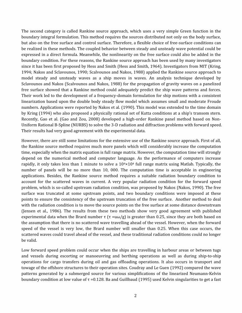
Fig. 2 shows the Doppler Shift of scattered wave field by a vessel travelling with constant forward speed u0

in the positive x direction. When a vessel is moving from point B to point O, the traveling time should be

t=BO/u0. During this period of time, the vessel produces scattered waves all along BO (the first scattered

wave should arise at point B). The control surface here is defined as a circle with its centroid on point O and

its radius as BO. If u0 is small, the travelling time t will be very long, which means the scattered waves

produced at point B can travel a long distance. When it just reaches point A, the wave group is reaching

point O (the wave group velocity is half of scattered wave velocity). In this case, the Brard number ぷ=0.25

(ぷ=u0ù/g), u0=uc (uc denotes the critical forward speed of the vessel at ぷ=0.25) and the scattered wave can

reach any points on the control surface. If ぷ<0.25 and u0<uc, the wave group will go head of the vessel.

Therefore, the upstream radiation condition could not be used any longer. If ぷ>0.25 and u0>uc, the scattered

wave can only get to point D, as shown in Fig. 3. On arc DA, there are no scattered waves reaching here, and

it is defined as SC2. To the contrary, arc BD is defined as SC1, on which a different radiation condition should

be imposed. From Fig. 3, the wave direction of a scattered wave reaching point D (x, y), which is produced

at B, have been rotated by an angle し (if there is no forward speed, the wave direction should be along OD.

The velocity of the scattered wave is defined as c, BO/u0=BD/c. According to the sine theorem, it can be

easily transferred to

2 2

0 sinx yu

c y

(13)

The scattered wave velocity at D can be expressed as

s

s

ck

(14)

ば

where ùs is the angular frequency of the scattered waves from a fixed reference point given as

1

0 cos[tan ] tanhs e s s s

yu k gk k d

x

(15)

in which ks is the local wave number at D(x, y), and d is the water depth.

Once the coordinates of any arbitrary point on the control surface are given, the unknowns し and ks could

be obtained by solving the nonlinear equation system (13)-(15). If one cannot find solutions, these points

must be on the control surface Sc2. Otherwise, they are on Sc1. The radiation condition is defined as two

different equations,

cos 0j

s jikn

(jサな┸ に┸ ┼ ┸ はょ on Sc1 (16)

0j (jサな┸ に┸ ┼ ┸ はょ on Sc2 (17)

Eq. (16) is an updated Sommerfeld radiation condition with forward speed correction. If the forward speed

is zero, ks=k , し =0 and Eq. (16) could reduce to the Sommerfeld radiation condition

0j

jikn

ゅjサな┸ に┸ ┼ ┸ 6) on Sc (18)

Fig. 4 Rectangle control surface

0

1

2

3

4

5

0 2 4 6 8 10 12 14 16 18 20

ks

Element number

Fn=0.0

Fn=0.1

Fn=0.2

Fn=0.3

ぱ

Fig. 5 Local wave number on rectangle control surface

Fig. 6 Circular control surface

Fig. 7 Local wave number on circular control surface

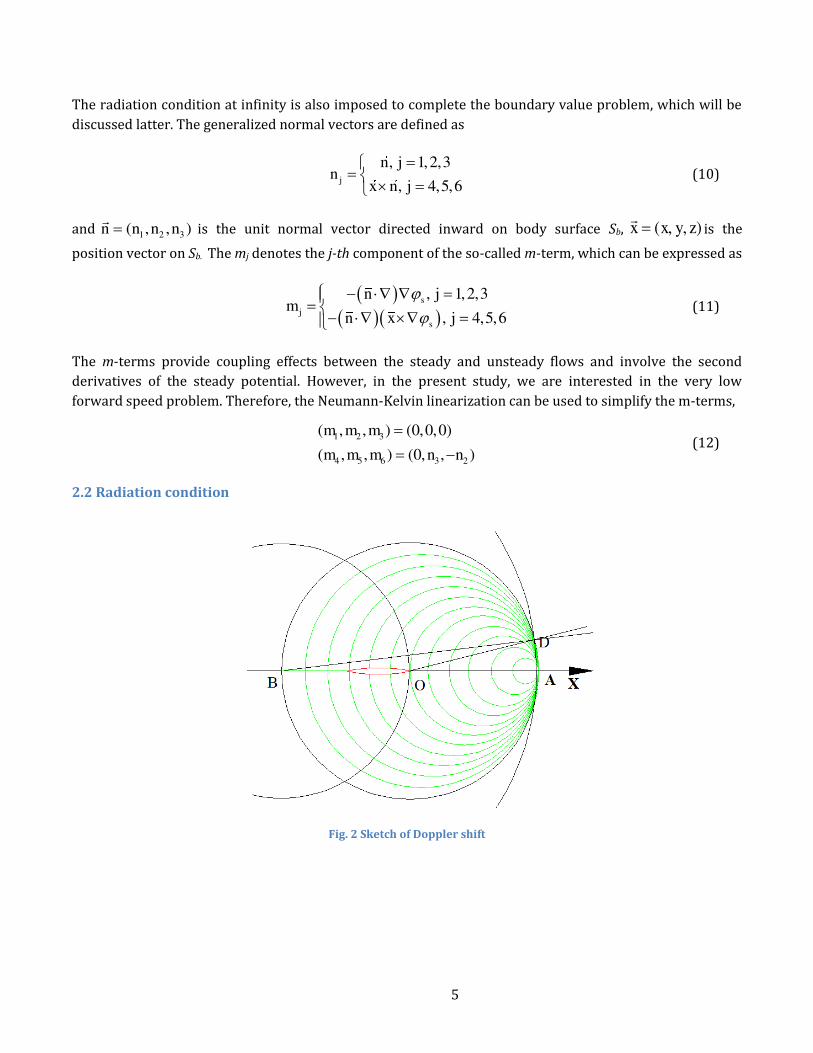
Fig. 4 and Fig. 6 show a Wigley hull traveling with different Froude number in the positive x direction and

the free surface is truncated by a rectangle and circular control surface respectively. The control surface is

dispersed into a series of discrete elements (20 elements in the present model). Fig. 5 and Fig. 7 are the

results of the local wave number ks on different control surfaces and different Froude numbers. ks =0

illustrates that no solution is found at these elements and these points are on SC2. It can be found from Fig. 5

that as the Froude number increases, the range of Sc1 shrinks. At Fnスね┸ ずスね and ks=k, which is a constant

independent of the location. When Fn=0.1, the scattered wave at B can only reach No.1-12 elements, and for

No.13-20 elements, no solution can be found here. When the Froude number increases to 0.3, only No.1-5

elements on the downstream end can be influenced by the scattered waves. The values of ks are inversely

proportional to the distance between B and the points on the control surface. Fig. 7 transmits the same

information as Fig. 5, which indicates that the truncation of free surface could be arbitrary and ks and ず are

only determined by the coordinates of the points on the control surface. However, in the numerical study,

the free surface range will greatly influence the computational results, and this will be discussed in the next

section.

2.3 Equations of motion

Once the unknown potential ぺs and ぺj are solved, the steady pressure and the time-harmonic pressure can be obtained from Bernoulli╆s equation┺

0

1

2

3

4

5

0 2 4 6 8 10 12 14 16 18 20

ks

Element number

Fn=0.0

Fn=0.1

Fn=0.2

Fn=0.3

ひ

0

1

2

ss s sp u

x

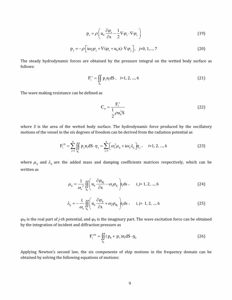
(19)

0( )j e j s jp i u x , j=0, な┸┼┸ 7 (20)

The steady hydrodynamic forces are obtained by the pressure integral on the wetted body surface as

follows:

b

s

i s i

S

F p n dS , i=1, 2, ┼┸ 6 (21)

The wave making resistance can be defined as

1

2

0

1

2

s

w

FC

u S (22)

where S is the area of the wetted body surface. The hydrodynamic force produced by the oscillatory

motions of the vessel in the six degrees of freedom can be derived from the radiation potential as

6 6

2

1 1b

D

i j i j e ij e ij j

j jS

F p n dS i

ˈ i=1, 2, ┼┸ 6 (23)

where ij and ij are the added mass and damping coefficients matrices respectively, which can be

written as

02

1

b

Rj

ij e Ij i

e S

u n dsx

ˈ i, jサ な┸ に┸ ┼┸ は (24)

0

1

b

Ij

ij e Rj i

e S

u n dsx

ˈ i┸ jサ な┸ に┸ ┼┸ は (25)

ぺRj is the real part of j-th potential, and ぺIj is the imaginary part. The wave excitation force can be obtained

by the integration of incident and diffraction pressure as

0 7 0( )

b

ext

i i

S

F p p n dS (26)

Applying Newton╆s second law┸ the six components of ship motions in the frequency domain can be obtained by solving the following equations of motions:

など

6

2

1

ext

e ij ij e ij ij j i

j

M i K F

(27)

The mass matrix Mij and restoring matrix coefficient Kij are given by

44 46

55

64 66

0 0 0 0

0 0 0

0 0 0 0

0 0 0

0 0 0

0 0 0

G

G G

G

ij

G

G G

G

m mz

m mz mx

m mxM

mz I I

mz mx I

mx I I

(28)

1

2

0 0 0 0 0 0

0 0 0 0 0 0

0 0 0 0

0 0 0 ( ) 0 0

0 0 0 ( ) 0

0 0 0 0 0 0

w w

ij

w B

w w B

gA gMK

g I Vz

gM g I Vz

(29)

where m is the body mass; (xG, yG, zG) is the center of gravity; I44, I55 and I66 are the roll, pitch and yaw

moments of inertia; the roll-yaw moment of inertia holds the symmetry relation I46= I64; Aw is the water

plane area; Mw is the first moment of the water plane about the y-axis; Iw1 and Iw2 are the second moment of

the water plane about the x-axis and y-axis respectively; V is the underwater volume; zB is the vertical

center of buoyancy.

The standard matrix solution routine provides the complex amplitude of the oscillatory motions from Eq.

(27). Then, the wave elevation can be obtained from the dynamic free surface boundary condition in the

form

7 7

0

0 0

1( ) ( )e

j j s j j

j j

iu x

g g

(30)

3 Numerical implementation

3.1 Discretization of the boundary integral

In the numerical study, the boundary is divided into a number of quadrilateral panels with constant source

density )(

, where ),,(

is the position vector on the boundary. If ),,( zyxx

is inside the fluid

domain or on the boundary surface, the potential can be expressed by a source distribution on the

boundary of the fluid domain:

なな

( ) ( ) ( , )

b f cS S S

x G x dS

(31)

where ぺ denotes the steady potential ぺs or the unsteady potential ぺj, ),(

xG is the Rankine-type Green

function given by

2 2 2

1( , )

( ) ( ) ( )G x

x y z

(32)

If we have N panels on the body surface, free surface and control surface together, the potential in point x

becomes

,

1 1

( ) ( , )4 4

b f c

N Nj j

i i i j

j jS S S

x G x dS G

(33)

When the collocation point and the panel are close to each other, the influence coefficients Gij can be

calculated with analytical formulas listed by Prins (1995) when the distance between the collocation point

and the panel is large, these coefficients are calculated numerically. The same procedure can be applied to

discretize the boundary integral for the velocity

,

1 1

1 1( ) ( , )

2 4 2 4b f c

N Nj j n

i i i i i j

j jiS S Sj i j i

x G x dS Gn n

(34)

The analytical formulas of the influence coefficients n

jiG , are listed by Hess and Smith (1964).

3.2 Desingularied method

The singularity distribution does not have to be located on the free surface itself, it can also be located at a

short distance above the free surface, as long as the collocation points, where the boundary condition has

to be satisfied, stay on the free surface. In practice, a distance of maximal three times the longitudinal size

of a panel is possible (Bunnik, 1999). In the present study, the raised distance ii Sz , where Si is the

area of the i-th panel.

Special attentions should be paid on the second derivative of the potential on the free surface. Generally,

the difference schemes can be divided in two classes: up wind difference schemes and central difference

schemes. Although central difference schemes are supposed to be more accurate, the stabilizing properties

of the upwind difference schemes are more desired in the forward speed problem (Bunnik, 1999).

Physically this can be explained by the face that new information on the wave pattern mainly comes from

the upstream side, especially at high speeds, whereas the downstream side only contains old information.

The first-order upwind difference scheme for the second derivative of the potential to x can be written as

follows

なに

2

2 12 2

1( ) ( ) 2 ( ) ( )i i i ix x x x

x x

(35)

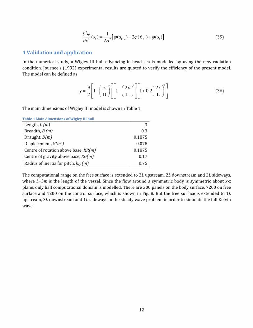
4 Validation and application

In the numerical study, a Wigley III hull advancing in head sea is modelled by using the new radiation condition┻ Journee╆s (1992) experimental results are quoted to verify the efficiency of the present model.

The model can be defined as

2 22 2

1 1 1 0.22

sB z x x

yD L L

(36)

The main dimensions of Wigley III model is shown in Table 1.

Table 1 Main dimensions of Wigley III hull

Length, L (m) 3

Breadth, B (m) 0.3

Draught, D(m) 0.1875

Displacement, V(m3) 0.078

Centre of rotation above base, KR(m) 0.1875

Centre of gravity above base, KG(m) 0.17

Radius of inertia for pitch, kyy (m) 0.75

The computational range on the free surface is extended to 2L upstream, 2L downstream and 2L sideways,

where L=3m is the length of the vessel. Since the flow around a symmetric body is symmetric about x-z

plane, only half computational domain is modelled. There are 300 panels on the body surface, 7200 on free

surface and 1200 on the control surface, which is shown in Fig. 8. But the free surface is extended to 1L

upstream, 3L downstream and 1L sideways in the steady wave problem in order to simulate the full Kelvin

wave.

なぬ

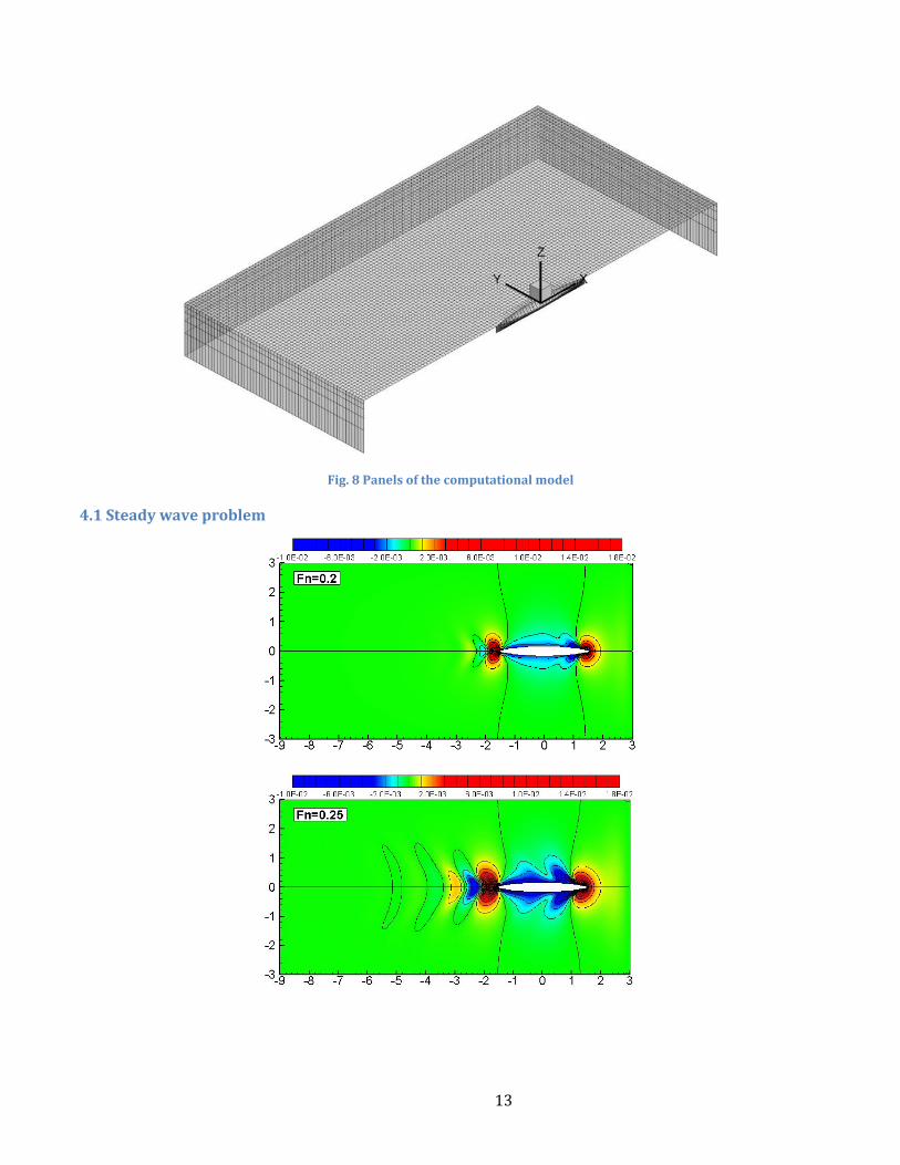
Fig. 8 Panels of the computational model

4.1 Steady wave problem

なね

Fig. 9 Steady wave pattern at various speeds

なの

Fig. 10 Wave making resistance of the Wigley hull

Fig. 9 shows the comparison of the wave pattern around the Wigley hull at different Froude numbers

( 0 /nF u gL ). As can be seen in these figures, the steady wave elevation attenuates rapidly behind the

ship. The diverging waves are radiating from the bow together with the transverse waves following behind

the stern. The Kelvin angle increases as the forward speed of the ship increases. At Fn= 0.2, the steady wave

elevation is very small, which means the energy dissipation is relatively small at low forward speed. This

can also be observed from the wave making resistance in Fig. 10. Compared with the ITTC experimental

results (SRI: Ship Research Institute, Tokyo; TOKYO: University of Tokyo), the present results based on the

steady flow is satisfactory. It can be found that in the very low forward speed region, the wave making

resistance is quite small.

4.2 The radiation problem

(a) Fn=0, ぷ=0 (b) Fn=0.037, ɒ=0.1

0

0.5

1

1.5

2

2.5

3

3.5

0 0.1 0.2 0.3 0.4 0.5 0.6Cw*1000

Fn

Present code

Exp. (SRI)

Exp. (TOKYO)

なは

(c) Fn=0.068, ɒ=0.2 (d) Fn=0.083, ɒ=0.25

(e) Fn=0.085, ɒ=0.26

Fig. 11 Radiation wave pattern induced by unit heave motion at very low forward speed

なば

(a) Fn=0.2, ɒ=0.75 (b) Fn=0.3, ɒ=1.32

Fig. 12 Radiation wave pattern induced by unit heave motion at medium forward speed

Fig. 11 and Fig. 12 are the radiation wave pattern induced by unit heave motion. The wave length to ship

length ratio of ぢ/L=1 in head sea corresponds to the critical conditions in ship design. In order to

investigate how the new double Doppler shift radiation condition changes the radiation wave pattern in

very low forward speed, we make the comparison between the present model and Sommerfeld radiation

condition over various range of Brard number from 0 to 1.32. The lower half of each sub-figure of Fig. 11

shows the wave pattern obtained from Sommerfield radiation condition, while the radiation condition in

the upper half account for the new double Doppler shift radiation condition defined by Eqs. (16)-(17). At

zero forward speed, the wave elevation calculated from present radiation condition is exactly the same as

that from Sommerfeld radiation condition. The waves propagate as a circle pattern beyond one wavelength

from the center with the main radiation energy on either side of the vessel. From Fig. 11 (b) and Fig. 11 (c)

we can find that even at very low forward speed, the Doppler shift becomes evident and it modifies the

wave length. The wave length downstream is larger than the upstream wave length. It can also be found

that if the new radiation condition associated with Doppler shift correction is used, the waves appear

smooth and stable. While for the Sommerfeld radiation condition, there are some distortions and

reflections from the control surface. As the Brard number increases to 0.25, or just a little greater than 0.25,

the forward speed of the vessel is equal to or greater than the wave group velocity. There should be no

waves propagating ahead of the vessel. This phenomenon could be illustrated well from Fig. 11 (d) and Fig.

11 (e). And also, the wave pattern is smooth and stable by using the new model. At Fn=0.2 and Fn=0.3, the

quiescent region ahead of the vessel expands, and the wave behaves as a V-shape downstream, which can

be seen from Fig. 12.

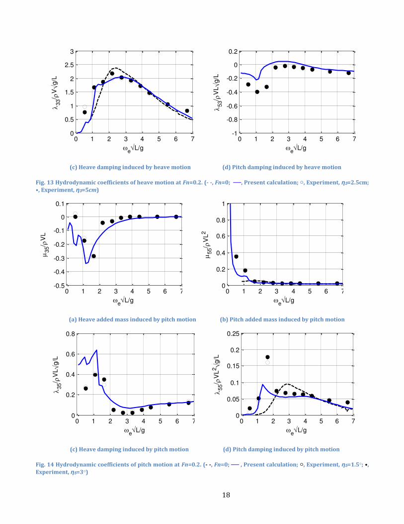
(a) Heave added mass induced by heave motion (b) Pitch added mass induced by heave motion

0 1 2 3 4 5 6 70

1

2

3

4

5

eL/g

33/

V

0 1 2 3 4 5 6 7-0.1

0

0.1

0.2

0.3

0.4

0.5

eL/g

53/

VL

なぱ

(c) Heave damping induced by heave motion (d) Pitch damping induced by heave motion

Fig. 13 Hydrodynamic coefficients of heave motion at Fn=0.2. (- -, Fn=0; —┸ Present calculation┹ 鯵┸ Experiment┸ Ș3=2.5cm;

ぇ┸ Experiment┸ Ș3=5cm)

(a) Heave added mass induced by pitch motion (b) Pitch added mass induced by pitch motion

(c) Heave damping induced by pitch motion (d) Pitch damping induced by pitch motion

Fig. 14 Hydrodynamic coefficients of pitch motion at Fn=0.2. (- -, Fn=0; — , Present calculation; 鯵, Experiment, Ș5=1.5鯵; ぇ,

Experiment, Ș5=3鯵)

0 1 2 3 4 5 6 70

0.5

1

1.5

2

2.5

3

eL/g

33/

Vg

/L

0 1 2 3 4 5 6 7-1

-0.8

-0.6

-0.4

-0.2

0

0.2

eL/g

53/

VLg

/L

0 1 2 3 4 5 6 7-0.5

-0.4

-0.3

-0.2

-0.1

0

0.1

eL/g

35/

VL

0 1 2 3 4 5 6 70

0.2

0.4

0.6

0.8

1

eL/g

55/

VL

2

0 1 2 3 4 5 6 70

0.2

0.4

0.6

0.8

eL/g

35/

VLg

/L

0 1 2 3 4 5 6 70

0.05

0.1

0.15

0.2

0.25

eL/g

55/

VL

2g

/L

なひ

Fig. 13 and Fig. 14 compare the hydrodynamic coefficients between the present calculations and

experimental results. Overall, the agreement is quite good in added mass and damping coefficients of heave

and pitch motion. Discrepancy arises near ぷ=0.25 ( 26.1/ gLe ). This phenomenon has also been

observed by Kim and Shin (2007) by using Green function method. The main reason for the difference lies

on the steady wave mj terms given by Eq. (11). In the present code, the free-stream assumption of Eq. (12)

is used and the coupling effects between the steady and unsteady flows have been neglected. However, this

m-term appeared in the body boundary condition will bring some influences to the radiation problem,

which is reflected in the hydrodynamic coefficients. In order to get better hydrodynamic coefficients, the

double-body or steady-wave flow should be taken as the basic flow. Experimental data for very low

forward speed is unfortunately not available.

4.3 The Diffraction problem

(a) Fn=0, ɒ=0 (b) Fn=0.037, ɒ=0.1

(c) Fn=0.068, ɒ=0.2 (d) Fn=0.083, ɒ=0.25

にど

(e) Fn=0.085, ɒ=0.26

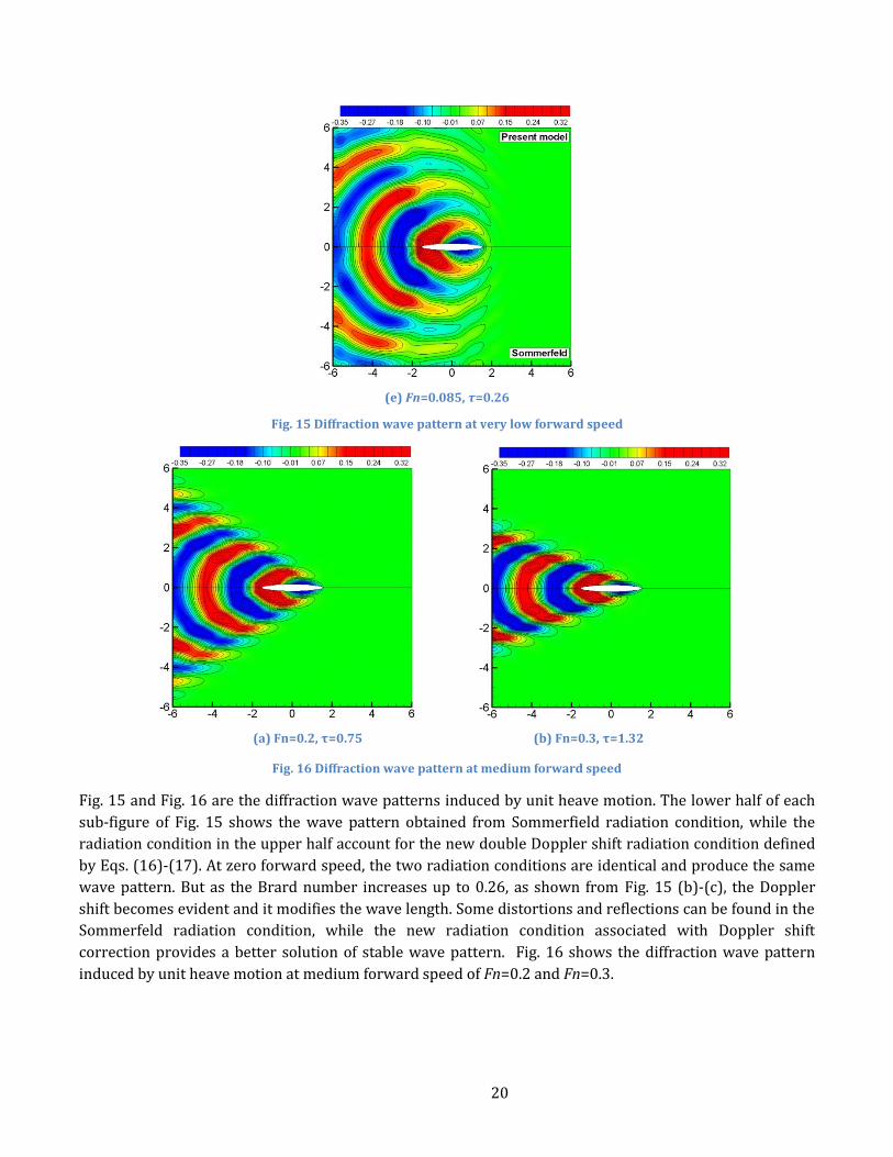
Fig. 15 Diffraction wave pattern at very low forward speed

(a) Fn=0.2, ぷ=0.75 (b) Fn=0.3, ぷ=1.32

Fig. 16 Diffraction wave pattern at medium forward speed

Fig. 15 and Fig. 16 are the diffraction wave patterns induced by unit heave motion. The lower half of each

sub-figure of Fig. 15 shows the wave pattern obtained from Sommerfield radiation condition, while the

radiation condition in the upper half account for the new double Doppler shift radiation condition defined

by Eqs. (16)-(17). At zero forward speed, the two radiation conditions are identical and produce the same

wave pattern. But as the Brard number increases up to 0.26, as shown from Fig. 15 (b)-(c), the Doppler

shift becomes evident and it modifies the wave length. Some distortions and reflections can be found in the

Sommerfeld radiation condition, while the new radiation condition associated with Doppler shift

correction provides a better solution of stable wave pattern. Fig. 16 shows the diffraction wave pattern

induced by unit heave motion at medium forward speed of Fn=0.2 and Fn=0.3.

にな

(a) (b)

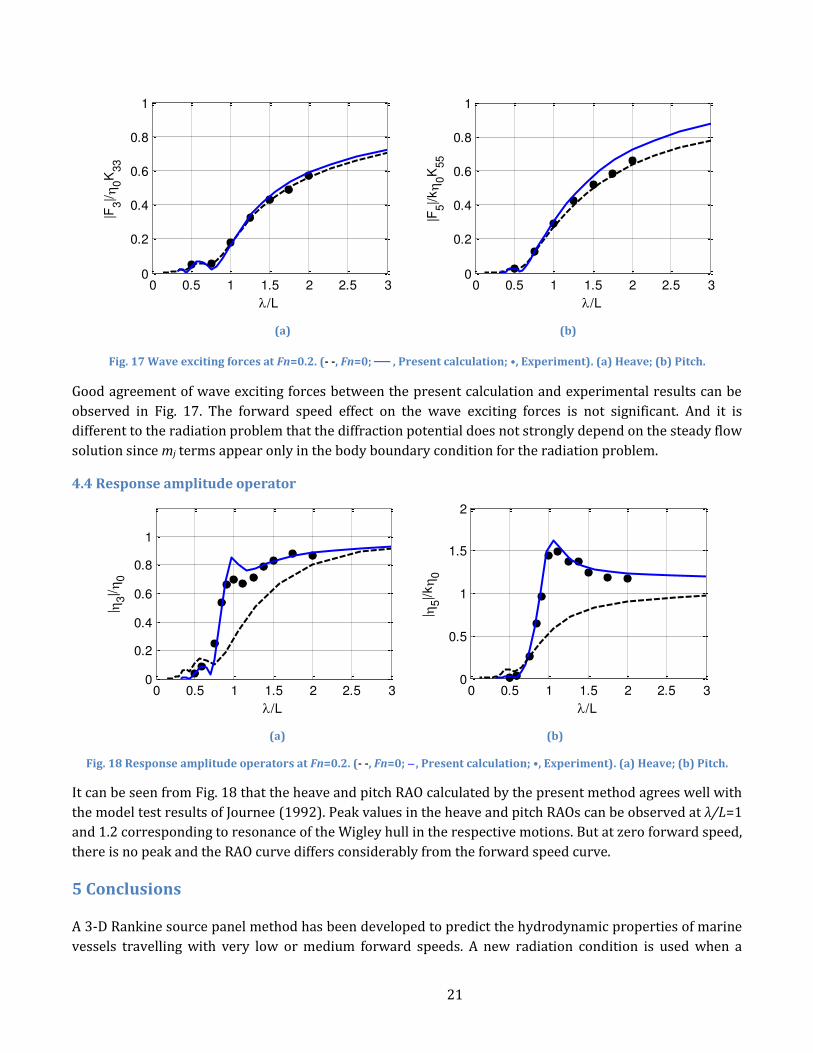
Fig. 17 Wave exciting forces at Fn=0.2. (- -, Fn=0; — , Present calculation; ぇ┸ Experimentょ. (a) Heave; (b) Pitch.

Good agreement of wave exciting forces between the present calculation and experimental results can be

observed in Fig. 17. The forward speed effect on the wave exciting forces is not significant. And it is

different to the radiation problem that the diffraction potential does not strongly depend on the steady flow

solution since mj terms appear only in the body boundary condition for the radiation problem.

4.4 Response amplitude operator

(a) (b)

Fig. 18 Response amplitude operators at Fn=0.2. (- -, Fn=0; 羽 , Present calculation┹ ぇ┸ Experimentょ. (a) Heave; (b) Pitch.

It can be seen from Fig. 18 that the heave and pitch RAO calculated by the present method agrees well with

the model test results of Journee (1992). Peak values in the heave and pitch RAOs can be observed at ぢ/L=1

and 1.2 corresponding to resonance of the Wigley hull in the respective motions. But at zero forward speed,

there is no peak and the RAO curve differs considerably from the forward speed curve.

5 Conclusions

A 3-D Rankine source panel method has been developed to predict the hydrodynamic properties of marine

vessels travelling with very low or medium forward speeds. A new radiation condition is used when a

0 0.5 1 1.5 2 2.5 30

0.2

0.4

0.6

0.8

1

/L

|F3|/ 0

K33

0 0.5 1 1.5 2 2.5 30

0.2

0.4

0.6

0.8

1

/L

|F5|/k 0

K55

0 0.5 1 1.5 2 2.5 30

0.2

0.4

0.6

0.8

1

/L

| 3|/ 0

0 0.5 1 1.5 2 2.5 30

0.5

1

1.5

2

/L

| 5|/k 0

にに

vessel moves with very low forward speed. This new radiation condition corrects the Sommerfeld radiation

condition by taking into account of Doppler shift. A Wigley III hull travelling with very low or medium

forward speed was considered to verify this radiation conditon. Comparing with the experimental data, the

following conclusions can be reached:

1) The new radiation condition associated with Doppler shift correction can provide a good solution of

scatterd wave pattern at very low forward speed. The wave field appears more stable and reasonable than

Sommerfeld radiation condition over a range of Brard number up to 0.26.

2) The present method is also effective to predict the hydrodynamic properties of the vessel travelling

with medium forward speed. The wave pattern at medium forward speed appears stable and there is no

reflection from the control surface. The calculated wave exciting forces and motion RAOs have a very good

agreement with the model test results. Small discrepancy appears in predicting the hydrodynamic

coefficients in radiation problem due to the coupled effects between the steady flow and radiation potential

being neglected, which should be taken into account in the body surface boundary condition in order to

obtain more accurate results. Overall, the agreement is found satisfactory.

6 Acknowledgments

The present work is mainly funded by Lloyd's Register┻ Authors are grateful to Lloyd╆s Register for their support.

7 References

Ba, M., Guillbaud, M., 1995. A fast method of evaluation for the translating and pulsating green's function.

Ship Technology Research 42 (2), 68-81.

Bunnik, T., 1999. Seakeeping calculations for ships, taking into account the non-linear steady waves, PhD

thesis. Delft University of Technology, The Netherlands.

Coudray, T., Le Guen, J.F., 1992. Validation of a 3-D Sea-Keeping Software, 4th CADMO, Madrid, pp. 443-460.

Das, S., Cheung, K.F., 2012a. Hydroelasticity of marine vessels advancing in a seaway. Journal of Fluids and

Structures 34, 271-290.

Das, S., Cheung, K.F., 2012b. Scattered waves and motions of marine vessels advancing in a seaway. Wave

Motion 49 (1), 181-197.

Gao, Z., Zou, Z., 2008. A NURBS-based high-order panel method for three-dimensional radiation and

diffraction problems with forward speed. Ocean Engineering 35 (11-12), 1271-1282.

Hess, J.L., Smith, A.M.O., 1964. Calculation of nonlifting potential flow about arbitrary three-dimensional

bodies. Journal of Ship Reaearch 8 (2), 22-44.

Jensen, G., Mi, Z.X., Söding, H., 1986. Rankine source methods for numerical solutions of steady wave

resistance problem, Proceedings of 16th Symposium on Naval Hydrodynamics, Berkeley, pp. 575-582.

Journee, J.M.J., 1992. Experiments and calculations on 4 Wigley hull forms in head waves, Report No. 0909.

Ship Hydromechanics Laboratory, Delft University of Technology, The Netherlands.

Kim, B., Shin, Y., 2007. Steady flow approximations in 3-D ship motion calculation. Journal of Ship Reaearch

51 (3), 229-249.

Kring, D.C., 1994. Time domain ship motions by a three-dimensional Rankine panel method, PhD Thesis.

MIT.

Lee, C.H., Sclavounos, P.D., 1989. Removing the irregular frequencies from integral equations in wave-body

interactions. Journal of Fluid Mechanics 207, 393-418.

にぬ

Nakos, D.E., 1990. Ship wave patterns and motions by a three dimensional Rankine panel method, PhD

Thesis. MIT.

Nakos, D.E., Sclavounos, P.D., 1990. Steady and unsteady ship wave patterns. Journal of Fluid Mechanics

215, 263-288.

Newman, J.N., 1985. Algorithms for the Free-Surface Green Function. Journal of Engineering Mathematics

28 (3), 57-67.

Newman, J.N., 1992. The Approximation of Free-Surface Green Function, Wave Asymptotics, in: Martin,

P.A.a.W., G.R. (Ed.), The Proceedings of the Meeting to Mark the Retirement of Professor Fritz Useel from

the Beyer Chair of Applied Mathematics in University of Manchester. Cambridge University Press, pp. 107‒135.

Noblesse, F., Hendrix, D., 1992. On the theory of potential flow about a ship advancing in waves. Journal of

Ship Reaearch 36 (1), 17-30.

Nossen, J., Grue, J., Palm, E., 1991. Wave forces on three-dimensional floating bodies with small forward

speed. Journal of Fluid Mechanics 227, 135-160.

Prins, H.J., 1995. Time domain calculations of drift forces and moments, PhD Thesis. Delft University of

Technology, The Netherlands.

Scalvounos, P.D., Nakos, D.E., 1988. Stability analysis of panel methods for free surface flows with forward

speed, 17th Symposium on Naval Hydrodynamics, Den Hague, Nederland.