Yu-chin Chen and Kwok Ping Tsang* - vtechworks.lib.vt.edu · WHAT DOES THE YIELD CURVE TELL US ABOUT EXCHANGE RATE PREDICTABILITY? Yu-chin Chen and Kwok Ping Tsang* Abstract—Since

WHAT DOES THE YIELD CURVE TELL US ABOUT EXCHANGE RATE

PREDICTABILITY?

Yu-chin Chen and Kwok Ping Tsang*

Abstract—Since the term structure of interest rates embodies informationabout future economic activity, we extract relative Nelson-Siegel (1987)factors from cross-country yield curve differences to proxy expectedmovements in future exchange rate fundamentals. Using monthly data forthe United Kingdom, Canada, Japan, and the United States, we show thatthe yield curve factors predict exchange rate movements and explainexcess currency returns one month to two years ahead. Our results providesupport for the asset pricing formulation of exchange rate determinationand offer an intuitive explanation to the uncovered interest parity puzzleby relating currency risk premiums to inflation and business cycle risks.

I. Introduction

DO the term structures of interest rates contain informa-tion about a country’s exchange rate dynamics? This

paper shows that the Nelson-Siegel factors extracted fromtwo countries’ relative yield curves can predict future ex-change rate changes and excess currency returns 1 to 24months ahead. When the domestic yield curve shifts downor becomes steeper by 1 percentage point relative to the for-eign one, home currency can depreciate by 3% to 4% oversubsequent months.1 Its excess return, currency return net ofinterest differentials, declines by even more. Since the Nel-son-Siegel factors have well-known macroeconomic inter-pretations and capture expected dynamics of future eco-nomic activity, our findings provide support for the assetpricing approach of exchange rate determination and implythat the currency risk premiums are driven by differentialexpectations about countries’ future output and inflation, forexample. Our results offer an intuitive explanation to theuncovered interest rate (UIP) puzzle.

Decades of exchange rate studies have uncovered manywell-known empirical puzzles, in essence failing to connectfloating exchange rates to their theoretical macroeconomicdeterminants, or fundamentals.2 From a theoretical stand-point, the nominal exchange rate should be viewed as an assetprice; however, the empirical validation of this view remains

elusive. This asset approach is consistent with a range ofstructural models and relates the nominal exchange rate tothe discounted present value of its expected future fundamen-tals, which can include cross-country differences in moneysupply, output, and inflation, among others. Because mea-suring market expectations is difficult, additional assump-tions, such as a linear driving process for the fundamentals,are typically imposed in order to relate the exchange rate toits currently observable fundamentals.3 The performanceof the resulting exchange rate equations is infamously dis-mal, especially at short time horizons of less than a year ortwo.

This paper contends that market expectations may bemore complicated than what econometricians can capturewith the simple driving processes commonly assumed. Assuch, previous empirical failure may be the result of usinginappropriate proxies for market expectations of future fun-damentals rather than the failure of the models themselves.We propose an alternative method to capture market expec-tations and test the asset approach by exploiting informationcontained in the shapes of the yield curves. Research on theterm structure of interest rates has long maintained that theyield curve contains information about expected future eco-nomic dynamics, such as monetary policy, output, and infla-tion. Extending this lesson to the international context, welook at cross-country yield curve differences and extractthree Nelson-Siegel (1987) factors—relative level, slope,and curvature—to summarize the expectation informationcontained therein. The Nelson-Siegel representation hasseveral advantages over the conventional no-arbitrage fac-tor yield curve models. It is flexible enough to adapt to thechanging shapes of the yield curve, and the model is parsi-monious and easy to estimate. It is also more successful indescribing the dynamics of the yield curve over time, whichis important to our goal of relating the evolution of the yieldcurve to movements in the expected exchange rate funda-mentals.4

We look at three currency pairs over the period August1985 to July 2005: the Canada dollar, the British pound,and the Japan yen relative to the U.S. dollar.5 In addition,

Received for publication March 8, 2009. Revision accepted for publica-tion July 8, 2011.

* Chen: University of Washington; Tsang: Virginia Tech.We thank Vivian Yue for providing us the yield curve data and Charles

Nelson, Dani Rodrik, Barbara Rossi, Richard Startz, Wen-Jen Tsay, twoanonymous referees, and seminar and conference participants at the SanFrancisco and Boston Federal Reserve Banks, Duke University, the Uni-versity of Kansas, and the Bank of Canada–ECB FX Workshop for valu-able comments. This work was partly undertaken while Y.-c.C. was a vis-iting scholar at Academia Sinica, and she gratefully acknowledges itshospitality as well as financial support from the National Science Councilof Taiwan.

The online appendices are available at http://www.mitpressjournals.org/doi/suppl/10.1162/REST_a_00231.

1 When the curvature of the domestic yield curve increases relative tothe foreign one, home currency will appreciate subsequently, though theresponse is not as robust.

2 Frankel and Rose (1995) offer a comprehensive summary of the var-ious difficulties confronting the empirical exchange rate literature. Sarno(2005) and Rogoff and Stavrakeva (2008) present more recent surveys.

3 See Engel and West (2005) and Mark (1995), among many others.4 The no-arbitrage models are often successful in fitting a cross-section

of yields but do not do as well in the dynamic setting (Duffee 2002). Die-bold, Li, and Yue (2008) show that by imposing an AR(1) structure onthe factors, the Nelson-Siegel model has strong forecasting power forfuture yield curves. In addition, as discussed in Diebold, Rudebusch, andAruoba (2006), the Nelson-Siegel model avoids potential misspecificationdue to the presence of temporary arbitrage opportunities in the bondsmarket.

5 We note that our results hold also for the other currency pair combina-tions in our sample. For ease of presentation, we provide results only rela-tive to the U.S. dollar in this paper.

The Review of Economics and Statistics, March 2013, 95(1): 185–205

� 2013 by the President and Fellows of Harvard College and the Massachusetts Institute of Technology

borrego

Typewritten Text

Copyright by the MIT Press. Chen, Yu-Chin; Tsang, Kwok Ping. "What does the yield curve tell us about exchange rate predictability?" Rev. Econ. Stat., 95 (1) (2013), pp. 185–205 doi:10.1162/REST_a_00231

with a different data set, we present corroborating resultsfor a more recent period—between January 1991 and May2011. Using zero-coupon yield data, we fit the three Nelson-Siegel relative factors to the yield differences between thethree countries and the United States at maturities rangingfrom three months to ten years. Our results show that allthree relative yield curve factors can help predict bilateralexchange rate movements and explain excess currencyreturns one month to two years ahead, with the slope factorbeing the most robust across currencies. We find that a 1 per-centage point rise in the slope or level factors of one countryrelative to another produces an annualized 3% to 4% appre-ciation of its currency subsequently, with the magnitude ofthe effect declining over the horizon. The responses ofexcess currency returns tend to be even larger. Movementsin the curvature factor have a much smaller effect onexchange rates of roughly one-to-one, and they are also theleast robust. We pay special attention to addressing theinference bias inevitable in our small sample long-horizonregressions, which we discuss in more detail in section III.6

Tying floating exchange rates to macroeconomic funda-mentals has been a long-standing struggle in internationalfinance. Our results suggest that to the extent that the yieldcurve is shaped by market expectations regarding futuremacroeconomic fundamentals, exchange rate movementsare not disconnected from fundamentals but relate to themvia a present value asset pricing relation. Moreover, ourresults have straightforward economic interpretations andoffer insight into the uncovered interest parity puzzle: theempirical regularity that the currencies of high interest ratecountries tend to appreciate subsequently rather thandepreciate according to the foreign exchange market effi-cient condition. In particular, we find that deviations fromUIP—excess currency returns—systematically respond tothe shape of the yield curves, which in turn capture marketperception of future inflation, output, and other macro indi-cators.7 Take, for example, our results showing that a flatterrelative yield curve or an upward shift in its overall levelpredicts subsequent home currency appreciation and a highhome currency risk premium. Since the flattening of theyield curve is typically considered a signal for an economicslowdown or a forthcoming recession, a flat domestic yieldcurve relative to the foreign one suggests that the expectedfuture growth at home is relatively low. In accordance withthe present value relation, home currency faces depreciationpressure as investors pull out and, ceteris paribus, appreci-

ates over time toward its long-term equilibrium value.8 Asimilar explanation can also be applied to the case of a largelevel factor, which reflects high expected future inflation.Both of these scenarios can induce higher perceived riskassociated with holding the domestic currency, as its payoffwould be negatively correlated with the marginal utility ofconsumption. This explains our observed rise in excesshome currency returns—the risk premium associated withdomestic currency holding.

The above intuition has clear implications for the UIPpuzzle. Since a rise in the short-term interest rate flattensthe slope of the yield curve or raises its overall level, bothwould imply a risk-premium increase. The home currencymay thus appreciate subsequently instead of depreciateaccording to UIP if the risk premium adjustment is largeenough. Although we do not explicitly model expectationsand perceived risks in this paper, our results are in accor-dance with simple economic intuitions. In fact, we showthat by augmenting standard UIP regressions with longer-maturity rates, the UIP puzzle can disappear. This suggeststhe puzzle is related to an omitted risk premium term embo-died in the rest of the yield curves.

Using data from the Survey of Professional Forecasters,we provide empirical support for the view that the U.S.yield curve factors are highly correlated, in the directionsdiscussed above, with investors’ reported expectationsabout future GDP growth and inflation in the United States,as well as with their reported levels of anxiety about animpending economic downturn.9 Given their ability to cap-ture market expectations, we conjecture that the success ofthe yield curve factors in predicting exchange rates mayalso be attributable to their real-time nature. Molodtsova,Nikolsko-Rzhevsky, and Papell (2008), for instance, esti-mate Taylor rules for Germany and the United States andfind strong evidence that higher inflation predicts exchangerate appreciation using real-time data but not revised data.Finally, we note that our approach is consistent with pre-vious research using the term structure of the exchange rateforward premiums or the relative yield spreads to predictfuture spot exchange rate, such as Frankel (1979), Claridaand Taylor (1997), and Clarida et al (2003).10 Yield differ-ences relate to exchange rate forwards via the covered inter-est parity condition. However, given that the exchange rate

6 To complement results presented in the main text, we also conductrolling out-of-sample forecasts to see how our yield curve model forecastsfuture exchange rate changes relative to the random walk forecasts andalso forecasts based on interest differentials of a single maturity. Ourmodel does not consistently outperform the two benchmarks considered.See the online appendix for details.

7 Deviations from UIP reflect both currency risk premium and expecta-tion errors. For presentational simplicity, we assume away systematicexpectation errors here, though they are clearly present empirically andour analyses would carry through without making this assumption (seeFroot & Frankel, 1989, and Chen, Tsang, & Tsay, 2010).

8 We note that this finding is contrary to the classic Dornbusch (1976)overshooting model, which predicts an immediate currency appreciationand subsequent depreciation in response to a higher interest rate. Ourresult is consistent with observations made in more recent papers, such asEichenbaum and Evans (1995), Gourinchas and Tornell (2004), and Clar-ida and Waldman (2008).

9 We limit the analysis here to the United States because comparablehigh-quality survey data are more difficult to obtain for the other coun-tries. We explore the role of surveyed expectations more fully in Chenet al. (2010).

10 Frankel (1979) incorporates long-term interest rates, proxying forlong-term inflation, in exchange rate models. Clarida et al. (2003) findthat the term structure of forward premiums can forecast future spot rates.See also Boudoukh, Richardson, and Whitelaw (2005) and de los Rios(2009).

186 THE REVIEW OF ECONOMICS AND STATISTICS

forwards are available up to only a year or so, our yieldcurve approach can capture a much wider range of relevantmarket information by looking at yields all the way up toten years or beyond.11

II. The Exchange Rates and the Yield Curves

Both the exchange rate and the yield curve rest atop dec-ades of prodigious research. This paper makes no pretenseof offering a comprehensive framework for jointly model-ing the two, though we do believe this is a worthwhileendeavor.12 In this section, we first present the standardworkhorse approach to modeling the nominal exchange rateas an asset price. We then propose that progress in the yieldcurve literature, namely, the empirical evidence that yieldcurves embody information about expected future dynamicsof key macroeconomic variables, can help improve on theapproach used in previous exchange rate estimations. Next,we offer a brief presentation of the Nelson-Siegel yieldcurve factors as a parsimonious way to capture the informa-tion in the entire yield curve while having a well-estab-lished connection with macroeconomic variables. Finally,we present a short discussion on excess returns and risk pre-mium, connecting our findings to the UIP literature.

A. The Present Value Model of Exchange Rate

The asset approach to exchange rate determination mod-els the nominal exchange rate as the discounted presentvalue of its expected future fundamentals, such as cross-country differences in monetary policy, output, and infla-tion. This present-value relation can be derived from var-ious exchange rate models that linearly relate log exchangerate, st, to its log fundamental determinants, ft, and itsexpected future value Etstþ1. The first classical example isthe workhorse monetary model developed by Mussa (1976)and explored extensively in subsequent papers. Based onmoney market equilibrium, uncovered interest parity, andpurchasing power parity, the monetary model can beexpressed as

st ¼ cft þ wEtstþ1; ð1Þ

where ft ¼ ðmt � m�t Þ � /ðyt � y�t Þ, m is money stock, y isoutput, * denotes foreign variables, and /, c, w (as well ask below) are parameters related to the income and interestelasticities of money demand. Variations of the monetary

model that capture price rigidities and short-term liquidityeffects expand the set of fundamentals to f M

t ¼ðmt � m�t Þ � byðyt � y�t Þ � biðit � i�t Þ þ bpðpt � p�t Þ, as inFrankel (1979). Solving equation (1) forward and imposingthe appropriate transversality condition, the nominal ex-change rate has the standard asset price expression, basedon information It at time t:

st ¼ kX1

j¼0wjEt ftþ1jItð Þ: ð2Þ

This present value expression, with alternative sets ofmodel-dependent fundamentals, serves as the starting pointfor standard textbook treatments and for many major contri-butions to the empirical exchange rate literature (Mark,1995; Engel & West, 2005).

Several recent papers emphasize the importance ofmonetary policy rules, especially the Taylor rule, in model-ing exchange rates.13 The Taylor rule model assumes thatthe monetary policy instruments, the home interest rate itand the foreign rate i�t , are set as follows:

it¼ lt þ byygapt þ bpp

et ;

i�t¼ l�t þ byy�;gapt þ bpp

�;et � dqt;

ð3Þ

where ygapt is the output gap, pe

t is the expected inflation, by,bp; d >0, and lt contains the inflation and output targets,the equilibrium real interest rate, and other omitted terms.The foreign corresponding variables are denoted with anasterisk, and following the literature, we assume the foreigncentral bank to explicitly target the real exchange rate orpurchasing power parity qt ¼ st � pt þ p�t in addition, withp denoting the overall price level.14 The efficient marketcondition for the foreign exchange markets, under rationalexpectations, equates cross-border interest differentials it�i�t with the expected rate of home currency depreciation,adjusted for the risk premium associated with home cur-rency holdings, qH:

it � i�t ¼ EtDstþ1 þ qHt : ð4Þ

Combining equations (3) and (4) and letting vt ¼ lt � l�t ;we have:

by ygapt � y�;gap

tð Þ þ bp pet � p�;et

� �þ d st � pt þ p�t� �

þ vt ¼ EtDstþ1 þ qHt : ð5Þ

Solving for st and rearranging terms, we arrive at an expres-sion equivalent to equation (1), with a different set of fun-damentals f TR1

t :

11 Our Nelson-Siegel framework is also more comprehensive than usingonly the term spreads (for example, the difference between ten-yearTreasury notes and three-month Treasury bills).

12 Bekaert, Wei, and Xing (2007) and Wu (2007) are recent examplesthat attempt to jointly analyze the uncovered interest parity and the expec-tation hypothesis of the term structure of interest rates. On the finance side,recent efforts using arbitrage-free affine or quadratic factor models havealso shown success in connecting the term structure with the dynamics ofexchange rates (see Inci & Lu, 2004). In contrast to these papers, our workhere emphasizes the macroeconomic connections between the yield curvesand the exchange rates through the use of the Nelson-Siegel factors. Chenand Tsang (2009) present a macro-finance model of the exchange rate.

13 See Engel and West (2005), Molodtsova and Papell (2008), andWang and Wu (2009) as examples.

14 For notation simplicity, we assume the home and foreign centralbanks to have the same weights by and bp.

187WHAT DOES THE YIELD CURVE TELL US ABOUT EXCHANGE RATE PREDICTABILITY

st ¼d

1þ dpt � p�t� �

� 1

1þ dby ygap

t � y�;gaptð Þ

�

þbp pet � p�;et

� �� qH

t þ vt

�þ 1

1þ dEtstþ1: ð6Þ

Here f TR1t ¼ pt � p�t

� �; ygap

t � y�;gaptð Þ; pe

t � p�;et

� �;qH

t

� �. As

Engel and West pointed out (2005), equation (6) can bereexpressed in the same general form as equation (1) butwith yet a different set of fundamentals f TR2

t :

st ¼ d it � i�t� �

þ d pt � p�t� �

� by ygapt � y�;gap

tð Þ� bp p�t � p�;et

� �þ 1� dð ÞqH

t � vt þ 1� dð ÞEtstþ1;

ð7Þ

with f TR2t ¼ it� i�t

� �; pt� p�t� �

; ygapt � y�;gap

tð Þ;�

pet � p�;et

� �;

qHt g. Both equations (6) and (7) can be solved forward,

leading to the asset pricing equation (2) with a different setof fundamentals f TR1

t or f TR2t .

Various structural exchange rate models, classical orTaylor rule-based, can deliver the net present value equa-tion where the exchange rate is determined by expectedfuture values of cross-country output, inflation, and interestrates. As we show in the next section, these are exactly themacroeconomic indicators for which the yield curvesappear to embody information.

Empirically, the nominal exchange rate is best approxi-mated by a unit root process, so we express equation (2) ina first-differenced form (e is expectation error):

Dstþ1 ¼ kX1

j¼1wjEt DftþjjIt

� �þ etþ1: ð8Þ

From here on, we deviate from the common approach in theliterature that imposes additional assumptions on the statisti-cal processes driving the fundamentals. Instead, we use theinformation in the yield curves to proxy the expected dis-counted sum on the right-hand side of equation (8).15

B. The Yield Curve and the Nelson-Siegel Factors

The yield curve or the term structure of interest ratesdescribes the relationship between yields and their time tomaturity. Traditional models of the yield curve posit that itsshape is determined by expected future paths of interest ratesand perceived future uncertainty (the risk premia). While theclassic expectations hypothesis is rejected frequently,research on the term structure of interest rates has convin-cingly demonstrated that the yield curve contains informa-tion about expected future economic conditions, such as out-put growth and inflation.16 Below we give a brief summary

of the Nelson-Siegel (1987) framework for characterizingthe shape of the yield curve and motivate our use of the rela-tive factors. We then summarize the findings of the macro-finance literature regarding the factors’ predictive content.

The Nelson-Siegel (1987) factors offer a succinctapproach to characterize the shape of the yield curve in thefollowing form,17

imt ¼ Lt þ St

1� e�km

km

� �þ Ct

1� e�km

km� e�km

� �; ð9Þ

where imt is the continuously compounded zero-couponnominal yield on an m-month bond and parameter k con-trols the speed of exponential decay.18 The three factorsLt; St; and Ct typically capture most of the information in ayield curve, with R2 usually close to 0.99.

C. The Yield Curve-Macro Linkage

There is a long history of using the term structure to pre-dict output and inflation.19 Mishkin (1990a, 1990b) showsthat the yield curve predicts inflation and that movements inthe longer end of the yield curve are mainly explained bychanges in expected inflation. Barr and Campbell (1997)use data from U.K. index-linked bonds and show that long-term expected inflation explains almost 80% of the move-ment in long yields. Estrella and Mishkin (1998) show thatthe term spread is correlated with the probability of a reces-sion, and Hamilton and Kim (2002) find that it can forecastGDP growth.

The more recent macro-finance literature connects theobservation that the short rate is a monetary policy instru-ment with the idea that yields of all maturities are risk-adjusted averages of expected short rates. This more struc-tural approach offers deeper insight into the relationshipbetween the yield curve factors and macroeconomicdynamics.20 Ang, Piazzesi, and Wei (2006) find that theterm spread (the slope factor) and the short rate (the sum oflevel and slope factors) outperform a simple AR(1) modelin forecasting GDP growth four to twelve quarters ahead.Using a New Keynesian model, Bekaert, Cho, and Moreno(2010) demonstrate that the level factor is mainly moved bychanges in the central bank’s inflation target, and monetarypolicy shocks dominate the movements in the slope andcurvature factors. Dewachter and Lyrio (2006) estimate an

15 Previous literature has attempted to use surveyed market expectationsas an alternative. See Frankel and Rose (1995), Sarno (2005), and Chenet al. (2010) for more discussion.

16 The expectations hypothesis expresses a long yield of maturity m asthe average of the current one-period yield and the expected one-periodyields for the upcoming m � 1 periods, plus a term premium. See Thorn-ton (2006).

17 Nelson-Siegel (1987) derive the factors by approximating the for-ward rate curve at a given time with a Laguerre function that is the pro-duct of a polynomial and an exponential decay term. This forward rate isthe (equal-root) solution to the second-order differential equation for thespot rates. A parsimonious approximation of the yield curve can then beobtained by averaging over the forward rates. The resulting function iscapable of capturing the relevant shapes of the empirically observed yieldcurves: monotonic, humped, or S-shaped.

18 We use zero-coupon bonds to avoid the coupon effect and theTreasuries to abstract away from default risks and liquidity concerns.Parameter k is set to 0.0609 as is standard in the literature.

19 See Estrella (2005) for a survey and explanations for why the yieldcurve predicts output and inflation.

20 See Diebold, Piazzesi, and Rudebusch (2005) for a short survey.


affine model for the yield curve with macroeconomic vari-ables. They find that the level factor reflects agents’ long-runinflation expectation, the slope factor captures the businesscycle, and the curvature represents the monetary stance ofthe central bank. Finally, Rudebusch and Wu (2007, 2008)contend that the level factor incorporates long-term inflationexpectations, and the slope factor captures the central bank’sdual mandate of stabilizing the real economy and keepinginflation close to its target. They provide macroeconomicunderpinnings for the factors and show that when agents per-ceive an increase in the long-run inflation target, the levelfactor will rise and the whole yield curve will shift up. Theslope factor is modeled using a Taylor rule, reacting to theoutput gap ygap

t and inflation pt. When the central bank tight-ens monetary policy, the slope factor rises, forecasting lowergrowth in the future.21 To capture the arguments in the vastliterature above, we provide a simple illustrative example ofhow the level and slope factors incorporate expectations offuture inflation and output dynamics in Appendix A1 (theappendices are in the online supplement).

Noting that the exchange rate fundamentals ( f Mt ; f

TR1t , or

f TR2t ) discussed in section II.A are in cross-country differ-

ences, we propose to measure the discounted present value onthe right-hand side of equation (8) with the cross-country dif-ferences in their yield curves. Assuming symmetry andexploiting the linearity in the factor loadings in equation (9),we fit three Nelson-Siegel factors of the relative level (LR

t ), therelative slope (SR

t ), and the relative curvature (CRt ) as follows:

imt � im�

t ¼ LRt þ SR

t

1� e�km

km

� �

þ CRt

1� e�km

km� e�km

� �þ em

t ; ð10Þ

where emt is fitting error. The relative factors, LR

t , SRt , and CR

t ,serve as a proxy for expected future fundamentals in ourexchange rate regressions. (We note that im

t is defined as theU.S. or home yield, so the relative factors are defined from theperspective of the United States relative to the other countries.)

D. Excess Currency Returns and the Risk Premium

To gain further insight into the UIP puzzle, we examinehow excess returns respond to expectations about futuremacroeconomic dynamics. Excess return, defined here forthe foreign currency, is the difference in the cross-countryyields adjusting for the relative currency movements:

rxtþm ¼ im�t � im

t þ Dstþm; ð11Þ

where the last term represents the percentage appreciationof foreign currency.

Under the assumptions that on aggregate, foreignexchange market participants are risk neutral and have

rational expectations, the efficient market condition for theforeign exchange market equates expected exchange ratechanges to cross-country interest rate differences over thesame horizon; this is the UIP condition. In ex post data,however, UIP is systematically violated over a wide rangeof currency-interest rate pairs as well as frequencies. Theleading explanations for this UIP puzzle point to either thepresence of time-varying risk premiums or systematicexpectation errors.22 We note that under the assumption ofrational expectations, excess return in equation (11) repre-sents the risk premium associated with foreign currencyholdings, qF, as expressed below:

Dstþm � imt � im�t

� �¼ qF

tþm þ etþm ¼ rxtþm ð12Þ

where etþm represents expectation error and would-be whitenoise under rational expectations.23 We examine how therisk premium adjusts to market expectations about futurerelative macroeconomic dynamics, as captured by the rela-tive factors.

III. Data and Estimation Strategies

A. Data Description

Our main sample consists of monthly data from August1985 to July 2005 for the United States, Canada, Japan, andthe United Kingdom of the following series:

� Zero-coupon bond yields for maturities 3, 6, 9, 12, 15,18, 21, 24, 30, 36, 48, 60 72, 84, 96, 108, and 120months, where the yields are computed using the Fama-Bliss (1987) methodology. The data set is from Die-bold, Li, and Yue (2008), and we use three-monthTreasury bills from Global Financial Data to fill insome of the missing observations.

� Exchange rate measured as the U.S. dollar price perunit of the foreign currency.24 A lower number meansan appreciation of the home currency, the USD. For allhorizons, we define exchange rate change as theannualized change of the log exchange rate s.

To supplement our main results and see whether our find-ings are robust over the financial crisis of 2008, we also usedata covering January 1991 to May 2011, which we obtainfrom the Bank of Canada, Bank of England, and the FederalReserve Economic Data (we do not have data on Japan).

We estimate equation (10) by OLS period by period toobtain times series of the relative Nelson-Siegel factors, LR

t ,SR

t , and CRt , for Canada, Japan, and the United Kingdom,

21 The literature does not provide a clear interpretation of the curvaturefactor, so we do not emphasize its macroeconomic linkage.

22 The peso problem is also a common explanation. See Engel (1996)and Sarno (2005) for surveys.

23 If we relax the assumption of rational expectations, qF would then re-present both risk premium and expectation errors.

24 The yields are reported for the second day of each month. We matchthe yield data at time t with the exchange rate of the last day of the pre-vious month (two days earlier).


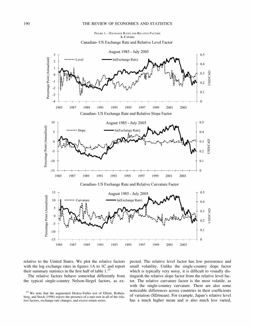
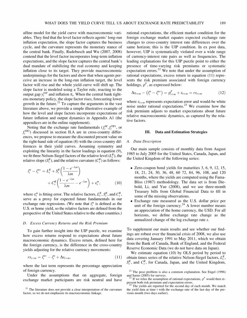
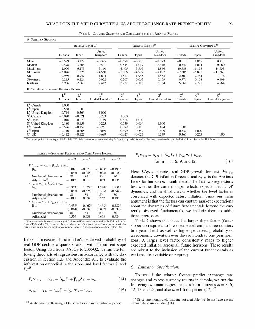
relative to the United States. We plot the relative factorswith the log exchange rates in figures 1A to 1C and reporttheir summary statistics in the first half of table 1.25

The relative factors behave somewhat differently fromthe typical single-country Nelson-Siegel factors, as ex-

pected. The relative level factor has low persistence andsmall volatility. Unlike the single-country slope factorwhich is typically very noisy, it is difficult to visually dis-tinguish the relative slope factor from the relative level fac-tor. The relative curvature factor is the most volatile, aswith the single-country curvature. There are also somenoticeable differences across countries in their coefficientsof variation (SD/mean). For example, Japan’s relative levelhas a much higher mean and is also much less varied,

FIGURE 1.—EXCHANGE RATES AND RELATIVE FACTORS

A. CANADA

25 We note that the augmented Dickey-Fuller test of Elliott, Rothen-berg, and Stock (1996) rejects the presence of a unit root in all of the rela-tive factors, exchange rate changes, and excess return series.


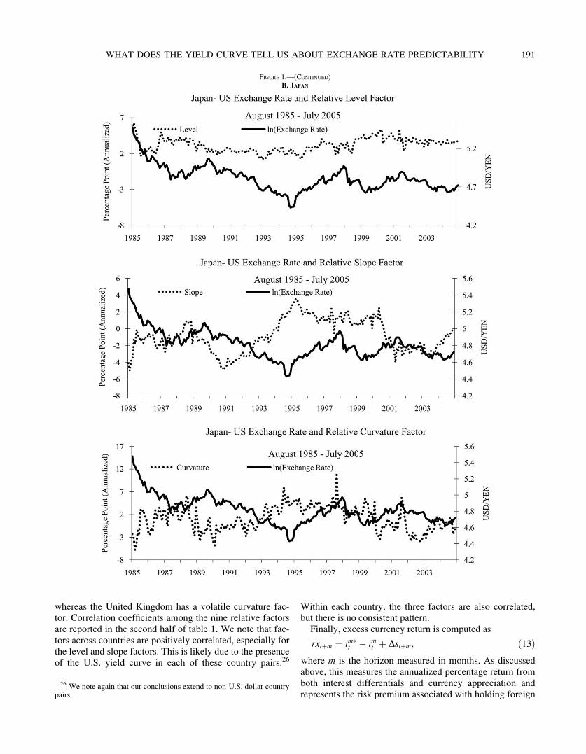
whereas the United Kingdom has a volatile curvature fac-tor. Correlation coefficients among the nine relative factorsare reported in the second half of table 1. We note that fac-tors across countries are positively correlated, especially forthe level and slope factors. This is likely due to the presenceof the U.S. yield curve in each of these country pairs.26

Within each country, the three factors are also correlated,but there is no consistent pattern.

Finally, excess currency return is computed as

rxtþm ¼ im�t � im

t þ Dstþm; ð13Þwhere m is the horizon measured in months. As discussedabove, this measures the annualized percentage return fromboth interest differentials and currency appreciation andrepresents the risk premium associated with holding foreign

FIGURE 1.—(CONTINUED)B. JAPAN

26 We note again that our conclusions extend to non-U.S. dollar countrypairs.


currency (under the assumption of no systematic expecta-tion errors, as discussed earlier).

B. Yield Curve Factors and Surveyed Expectations

Section II summarized prior research showing the termstructure factors as a robust and powerful predictor forfuture macroeconomic dynamics. We conduct some simpletests here using our U.S. yield curve data and the Survey ofProfessional Forecasters (SPF), which contains forecasts of

a wide range of economic indicators for the United Statesfrom a large group of private sector and institutional econo-mists.27 We take the mean forecasts for real GDP growthand CPI inflation for horizons from one to four quartersahead and correlate them with the current yield curve fac-tors. We also check the correspondence of the Anxious

FIGURE 1.—(CONTINUED)C. UNITED KINGDOM

The term structure factors for each country are calculated by the following procedure. In each period, we subtract the yields of each country from those of the United States, matching the maturities. We then fit theNelson-Siegel yield curve on the yield differences and obtain the level, slope, and curvature factors for that period.

27 We note that comparably reliable surveyed expectation data are diffi-cult to obtain for the other countries in our paper; hence, this section looksat the United States only.


Index—a measure of the market’s perceived probability ofreal GDP decline k quarters later—with the current slopefactor. Using data from 1985Q3 to 2005Q2, we run the fol-lowing three sets of regressions, in accordance with the dis-cussion in section II.B and Appendix A1, to evaluate theinformation embodied in the slope and level factors St andLt:

28

EtDytþm ¼ aSm þ bSmSt þ bymDyt þ uSmt; ð14Þ

Atþm ¼ cSm þ dSmSt þ dymDyt þ vSmt; ð15Þ

Etptþm ¼ aLm þ bLmLt þ bpmpt þ uLmt;

for m ¼ 3; 6; 9; and 12: ð16Þ

Here EDytþm denotes real GDP growth forecast, Eptþm

denotes the CPI inflation forecast, and Atþm is the AnxiousIndex for horizon m-month ahead. The first two regressionstest whether the current slope reflects expected real GDPdynamics, and the third checks whether the level factor iscorrelated with expected future inflation. Since our mainargument is that the factors can capture market expectationsabout the dynamics of future fundamentals beyond the cur-rently observed fundamentals, we include them as addi-tional regressors.

Table 2 shows that indeed, a larger slope factor (flatterslope) corresponds to lower expected output three quartersto a year ahead, as well as higher perceived probability ofan economic downturn over the six-month to one-year hori-zons. A larger level factor consistently maps to higherexpected inflation across all future horizons. These resultsare robust to the inclusion of the current fundamentals aswell (results available on request).

C. Estimation Specifications

To see if the relative factors predict exchange ratechanges and excess currency returns in sample, we run thefollowing two main regressions, each for horizons m ¼ 3, 6,12, 18, and 24, and also m ¼1 for equation (17):29

TABLE 1.—SUMMARY STATISTICS AND CORRELATIONS FOR THE RELATIVE FACTORS

A. Summary Statistics

Relative Level LR Relative Slope SR Relative Curvature CR

Canada JapanUnited

Kingdom Canada JapanUnited

Kingdom Canada JapanUnited

Kingdom

Mean �0.599 3.179 �0.395 �0.678 �0.826 �2.273 �0.611 1.055 0.417Median �0.598 3.208 �0.591 �0.515 �1.017 �2.446 �0.740 1.014 �0.260Maximum 2.000 6.279 3.110 4.406 3.567 2.946 10.589 11.138 14.938Minimum �3.076 1.225 �4.560 �5.306 �4.997 �7.097 �7.205 �5.821 �11.563SD 0.969 0.947 1.604 1.827 1.955 1.933 2.561 2.754 4.476Skewness 0.215 0.224 0.032 0.207 0.063 0.159 0.771 0.108 0.809Kurtosis 2.906 2.663 2.412 2.752 2.116 2.784 5.660 2.721 4.264

B. Correlations between Relative Factors

LR

CanadaLR

JapanLR

United KingdomSR

CanadaSR

JapanSR

United KingdomCR

CanadaCR

JapanCR

United Kingdom

LR Canada 1.000LR Japan 0.588 1.000LR United Kingdom 0.714 0.566 1.000SR Canada �0.080 �0.021 0.223 1.000SR Japan 0.046 �0.070 0.149 0.624 1.000SR United Kingdom �0.180 �0.153 �0.225 0.639 0.664 1.000CR Canada �0.586 �0.159 �0.261 0.079 0.113 0.084 1.000CR Japan �0.110 �0.265 �0.069 0.399 0.559 0.509 0.330 1.000CR UK �0.412 �0.122 �0.689 �0.027 �0.027 0.339 0.361 0.255 1.000

The sample period is from August 1985 to July 2005. Relative factors are estimated using OLS period by period for each of the three countries relative to the United States. See section IIIA for details.

TABLE 2.—SURVEYED FORECASTS AND YIELD CURVE FACTORS

m ¼ 3 m ¼ 6 m ¼ 9 m ¼ 12

EtDytþm ¼ aSm þ bSmSt þ uSmt

bSm 0.016 �0.073 �0.083* �0.192*(0.065) (0.048) (0.034) (0.038)

Number of observations 80 80 80 80Adjusted R2 �0.012 0.017 0.059 0.235

Atþm ¼ cSm þ dSmSt þ vSmt

dSm �0.352 1.078* 1.830* 1.950*(0.857) (0.526) (0.335) (0.344)

Number of observations 80 80 80 80Adjusted R2 �0.011 0.039 0.267 0.283

Etptþm ¼ aLm þ bLmLt þ uLmt

bLm 0.458* 0.462* 0.468* 0.482*(0.044) (0.039) (0.037) (0.037)

Number of observations 80 80 80 80Adjusted R2 0.579 0.638 0.663 0.684

We use quarterly data from the Survey of Professional Forecasters maintained by the Federal ReserveBank of Philadelphia. The factors are the quarterly average of the monthly data (though we obtain similarresults when we use the first month of each quarter instead). *Indicates significance level below 10%.

28 Additional results using all three factors are in the online appendix.

29 Since one-month yield data are not available, we do not have excessreturn data to run equation (18).


Dstþm ¼ bm;0 þ bm;1LRt þ bm;2SR

t þ bm;3CRt

þ utþm; ð17Þ

rxtþm ¼ cm;0 þ cm;1LRt þ cm;2SR

t þ cm;3CRt þ vtþm: ð18Þ

We note that for the United Kingdom, the relationshipbetween the two dependent variables and the relative factorsduring the exchange rate mechanism (ERM) crisis differs sig-nificantly from the rest of the sample.30 So in our analysis, wedrop the period October 1990 to September 1992, when the cri-sis was in effect, from the regressions for the United Kingdom.

It is well known that longer-horizon predictive analysesare prone to inference bias from using overlapping data.When the horizon for exchange rate change or excess cur-rency return is more than one month, our left-hand-side vari-able overlaps across observations, and utþm or vtþm in equa-tions (17) and (18) will be a moving-average process oforder m� 1. Statistics such as the standard errors will bebiased. One common solution is to use the Newey-West stan-dard errors. However, the Newey-West adjustment suffersfrom serious size distortion (it rejects too often) when thesample size is small and the regressors are persistent. Weaddress the problem using two alternative methods. The firstmethod uses critical values constructed from Monte Carlosimulations (discussed in the online appendix). For the restof the paper, we correct the long-horizon bias using therescaled t statistic suggested by Moon, Rubia, and Valkanov(2004) and Valkanov (2003), as it delivers more conserva-tive inferences than the Monte Carlo results. As discussed inAppendix A1, Moon et al. (2004) propose to rescale standardt-statistics by 1=

ffiffiffiffimp

and show that this rescaled t-statistic isapproximately standard normal, provided that the regressorxt is highly persistent. When the regressor is not a near-inte-grated process, however, the adjusted t-statistic tends to

underreject the null. Since the unit root null is rejected formost of our factors, we note that the predictive power of thefactors may actually be stronger than implied by the resultswe present in tables 3 to 5.31

IV. Main Results

A. Predictive Regressions

Our main exchange rate predictive results based on equa-tion (17) are presented in panel A of tables 3 to 5, with thecorresponding results for excess returns, equation (18), inpanel B. As a robustness check, we use the first month ofeach quarter and each half-year to construct a three-monthand a six-month sample with no data overlap. We report thefindings using the nonoverlapping data in table 6.

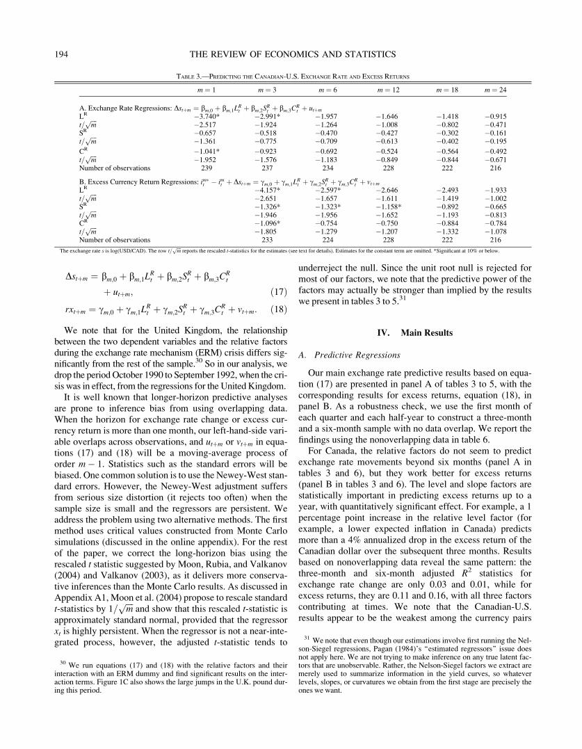
For Canada, the relative factors do not seem to predictexchange rate movements beyond six months (panel A intables 3 and 6), but they work better for excess returns(panel B in tables 3 and 6). The level and slope factors arestatistically important in predicting excess returns up to ayear, with quantitatively significant effect. For example, a 1percentage point increase in the relative level factor (forexample, a lower expected inflation in Canada) predictsmore than a 4% annualized drop in the excess return of theCanadian dollar over the subsequent three months. Resultsbased on nonoverlapping data reveal the same pattern: thethree-month and six-month adjusted R2 statistics forexchange rate change are only 0.03 and 0.01, while forexcess returns, they are 0.11 and 0.16, with all three factorscontributing at times. We note that the Canadian-U.S.results appear to be the weakest among the currency pairs

TABLE 3.—PREDICTING THE CANADIAN-U.S. EXCHANGE RATE AND EXCESS RETURNS

m ¼ 1 m ¼ 3 m ¼ 6 m ¼ 12 m ¼ 18 m ¼ 24

A. Exchange Rate Regressions: Dstþm ¼ bm;0 þ bm;1LRt þ bm;2SR

t þ bm;3CRt þ utþm

LR �3.740* �2.991* �1.957 �1.646 �1.418 �0.915t=

ffiffiffiffimp

�2.517 �1.924 �1.264 �1.008 �0.802 �0.471SR �0.657 �0.518 �0.470 �0.427 �0.302 �0.161t=

ffiffiffiffimp

�1.361 �0.775 �0.709 �0.613 �0.402 �0.195

CR �1.041* �0.923 �0.692 �0.524 �0.564 �0.492t=

ffiffiffiffimp

�1.952 �1.576 �1.183 �0.849 �0.844 �0.671Number of observations 239 237 234 228 222 216

B. Excess Currency Return Regressions: im�t � imt þ Dstþm ¼ cm;0 þ cm;1LR

t þ cm;2SRt þ cm;3CR

t þ vtþm

LR �4.157* �2.597* �2.646 �2.493 �1.933t=

ffiffiffiffimp

�2.651 �1.657 �1.611 �1.419 �1.002SR �1.326* �1.323* �1.158* �0.892 �0.665t=

ffiffiffiffimp

�1.946 �1.956 �1.652 �1.193 �0.813CR �1.096* �0.754 �0.750 �0.884 �0.784t=

ffiffiffiffimp �1.805 �1.279 �1.207 �1.332 �1.078

Number of observations 233 224 228 222 216

The exchange rate s is log(USD/CAD). The row t=ffiffiffiffimp

reports the rescaled t-statistics for the estimates (see text for details). Estimates for the constant term are omitted. *Significant at 10% or below.

30 We run equations (17) and (18) with the relative factors and theirinteraction with an ERM dummy and find significant results on the inter-action terms. Figure 1C also shows the large jumps in the U.K. pound dur-ing this period.

31 We note that even though our estimations involve first running the Nel-son-Siegel regressions, Pagan (1984)’s ‘‘estimated regressors’’ issue doesnot apply here. We are not trying to make inference on any true latent fac-tors that are unobservable. Rather, the Nelson-Siegel factors we extract aremerely used to summarize information in the yield curves, so whateverlevels, slopes, or curvatures we obtain from the first stage are precisely theones we want.


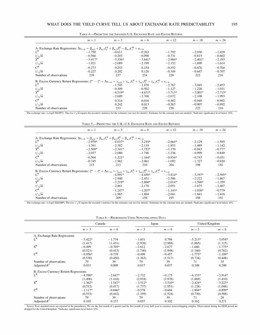
TABLE 6.—REGRESSIONS USING NONOVERLAPPING DATA

Canada Japan United Kingdom

m ¼ 3 m ¼ 6 m ¼ 3 m ¼ 6 m ¼ 3 m ¼ 6

A. Exchange Rate RegressionsLR �3.422* �1.734 �1.651 0.786 �5.213* �3.054*

(1.417) (1.431) (2.926) (2.968) (1.865) (1.115)SR �0.499 �0.705* �2.612 �2.677 �1.660 �1.775*

(0.521) (0.415) (1.740) (1.948) (1.160) (0.762)CR �0.956* �0.739 �0.499 �0.457 �1.773* �1.109*

(0.530) (0.450) (1.363) (1.517) (0.734) (0.448)Number of observations 79 39 79 39 71 35Adjusted R2 0.031 0.009 0.017 0.037 0.108 0.200

B. Excess Currency Return RegressionsLR �4.590* �2.647* �2.722 �0.175 �6.153* �3.914*

(1.406) (1.416) (2.918) (2.978) (1.869) (1.410)SR �1.362* �1.547* �3.512* �3.510* �2.424* �3.223*

(0.512) (0.417) (1.737) (1.951) (1.128) (1.048)CR �1.117* �0.846* �0.578 �0.604 �1.904* �0.899*

(0.533) (0.442) (1.359) (1.524) (0.730) (0.588)Number of observations 79 39 79 39 71 28Adjusted R2 0.105 0.157 0.057 0.102 0.162 0.271

Newey-West standard errors are reported in the parentheses. We use the first month of a quarter and the first month of every half-year to construct nonoverlapping samples. Observations during the ERM period aredropped for the United Kingdom. *Indicates significance level below 10%.

TABLE 5.—PREDICTING THE U.K.-U.S. EXCHANGE RATE AND EXCESS RETURNS

m ¼ 1 m ¼ 3 m ¼ 6 m ¼ 12 m ¼ 18 m ¼ 24



LR �2.970* �4.037* �3.210* �2.664* �2.129 �1.585t=

ffiffiffiffimp �1.761 �2.382 �2.119 �1.853 �1.489 �1.142

SR �2.509* �2.341* �1.752* �1.170 �0.943 �0.777t=

ffiffiffiffimp �2.037 �2.080 �1.746 �1.236 �0.999 �0.840

CR �0.504 �1.221* �1.164* �0.934* �0.743 �0.451t=

ffiffiffiffimp

�0.745 �1.962 �2.061 �1.692 �1.327 �0.820Number of observations 215 213 210 204 198 192



t þ vtþm

LR �4.991* �4.450* �3.814* �3.197* �2.595*t=

ffiffiffiffimp

�2.940 �2.451 �2.586 �2.222 �1.867SR �3.219* �2.860* �2.014* �1.590* �1.359t=

ffiffiffiffimp �2.861 �2.178 �2.051 �1.675 �1.467

CR �1.247* �1.207* �1.143* �1.038* �0.779t=

ffiffiffiffimp

�1.965 �1.804 �2.041 �1.841 �1.416Number of observations 209 159 195 198 192

The exchange rate s is log(USD/GBP). The row t=ffiffiffiffimp

reports the rescaled t-statistics for the estimates (see text for details). Estimates for the constant term are omitted. *Indicates significance level below 10%.

TABLE 4.—PREDICTING THE JAPANESE-U.S. EXCHANGE RATE AND EXCESS RETURNS

m ¼ 1 m ¼ 3 m ¼ 6 m ¼ 12 m ¼ 18 m ¼ 24



LR �1.750 �0.611 �0.263 �1.792 �2.030 �1.429t=

ffiffiffiffimp

�0.566 �0.203 �0.090 �0.731 �0.815 �0.602SR �3.417* �3.556* �3.641* �2.984* �2.401* �2.193t=

ffiffiffiffimp

�1.921 �2.089 �2.199 �2.152 �1.690 �1.614

CR �0.273 0.253 0.154 �0.352 �0.676 �0.704t=

ffiffiffiffimp

�0.227 0.202 0.126 �0.344 �0.647 �0.707Number of observations 239 237 234 228 222 216



t þ vtþm

LR �1.545 �1.470 �2.767 �3.045 �2.453t=

ffiffiffiffimp

�0.509 �0.502 �1.127 �1.220 �1.031SR �4.519* �4.631* �3.713* �3.001* �2.715*t=

ffiffiffiffimp

�2.609 �2.768 �2.672 �2.108 �1.993

CR 0.314 0.016 �0.582 �0.949 �0.992t=

ffiffiffiffimp

0.242 0.013 �0.567 �0.907 �0.992Number of observations 233 228 228 222 216

The exchange rate s is log(USD/JPY). The row t=ffiffiffiffimp

reports the rescaled t-statistics for the estimates (see text for details). Estimates for the constant term are omitted. *Indicates significance level below 10%.


we examined, with the predictability dissipating quicklyafter six months. Our conjecture is that this is mainly due tothe Canadian dollar’s commodity currency status, as dis-cussed previously in the literature.32

For Japan, the relative slope factor plays both a statisti-cally and an economically strong role in predicting theyen-dollar movements. As shown in table 4, panel A, a 1percentage point increase in the relative slope factor (theJapanese yield curve becomes steeper relative to the U.S.one, reflecting, for example, stronger Japanese growth pro-spects) predicts a 3.6% annualized depreciation of the yenover the next three months. In panel B, the same 1% increasein the relative slope factor predicts a 4.5% drop in excessyen returns over the U.S. dollar in the three-month horizon.The same pattern can be observed over horizons up to twoyears. These results make intuitive sense: during periods inwhich the Japanese relative growth prospect is high (com-pared to the sample average), the yen should be strong andinvestors would demand less risk premium for holding yen.Subsequently, the yen depreciates toward its equilibriumvalue (sample average). Interestingly, we do not find statisti-cally significant results for the other two relative factors.

For the United Kingdom, table 5 shows that all threeNelson-Siegel factors predict exchange rate changes andex-post excess returns with quantitatively and statisticallysignificant impact. A one percentage point increase in therelative level factor (the whole yield curve of the UnitedStates shifts up by one percentage point relative to that ofthe United Kingdom) predicts a 4% depreciation of thepound against the dollar and a 5% drop in the excess ster-ling return over the subsequent quarter. The explanatorypower of the relative factors for ex-post excess return infact extends beyond two years (not shown). The nonover-lapping results in table 6 confirm the relative factors’importance. The three-month and six-month adjusted R2

statistics for exchange rate change are 0.11 and 0.20, andfor excess return they are 0.16 and 0.27. We note that theseare high numbers; they contrast sharply with the view thatexchange rates are disconnected from macrofundamentals.

Overall, we see that for all three currency pairs, the rela-tive yield curve factors can play a quantitatively and statisti-cally significant role in explaining future exchange ratemovements over future intervals ranging from one month totwo years. We also observe a consistent pattern across cur-rency pairs: the effects of the factors, as captured by the sizeof the regression coefficients, tend to approach 0 as the fore-cast horizon increases. We view this as an indication thatcurrent information and expectations have a declining effecton the actual exchange rate realization further into the future;however, imprecision in the estimates and likely bias fromnoise in longer-horizon data prevent any conclusive state-

ment. (We present parallel results based on more recent datacovering January 1991 to May 2011 in the online appendix.)

B. Comparison with Interest Differential Regressions

Given our positive results, a natural question is how ourfactor model, using information contained in the full yieldcurves, compares to specifications using interest differen-tials of only one (for example, UIP) or two maturities(Frankel 1979). Below we present the discussion using theUIP regression as an example, though the logic applies toother cases as well.

The UIP puzzle originates from observing a negative andoften significantly estimated coefficient b in the followingregression setup for m in the one-year range:

Dstþm ¼ aþ b imt � im�

t

� �þ etþm: ð19Þ

While it implies that exchange rate change is predictable byinterest rate differentials, we note that this in-sample pre-dictability is consistent with exchange rate disconnect, orMeese-Rogoff (1983) random walk results, as the explana-tory power of interest differences is typically extremelysmall.33 How does our Nelson-Siegel (NS) factor approachrelate to the UIP regression? Intuitively, our yield curveapproach augments the m-period UIP regression with yielddifferences of all other maturities. Given the estimation pro-blem associated with having many highly collinear regres-sors, the NS factors serve as a parsimonious way to reducedimension, with the additional benefit of having well-estab-lished macroeconomic interpretations.

Mathematically, it is also easy to see that equation (19) isa constrained version of our factor model, equation (17).Substituting the formula for the relative Nelson-Siegel yieldcurve equation (10) into equation (19) and rearrangingterms, the UIP regression takes the following form:

Dstþm ¼ aþ bLRt þ b

1� exp �kmð Þkm

� �SR

t

þ b1� exp �kmð Þ

km� exp �kmð Þ

� �CR

t þ etþm: ð20Þ

This shows that the UIP regression is a constrained versionof our model, equation (17), with the following two horizon(m)-dependent restrictions:

b2;m

b1;m

¼ 1� exp �kmð Þkm

� �;

b3;m

b1;m

¼ 1� exp �kmð Þkm

� exp �kmð Þ� �

: ð21Þ

Since our model encompasses the UIP regression, we canformally test whether these restrictions are supported in the

32 The Canadian dollar is known to respond chiefly to the world price ofthe country’s primary commodity exports (see Chen & Rogoff, 2003, forfurther discussion on commodity currencies) In addition, Krippner (2006)found that the failure of the UIP in the CAD/USD rate is associated withthe cyclical component of Canadian interest rates.

33 Fama (1984) reports an average R2 of 0.01 for monthly data; see alsoChinn (2006) and Chinn and Meredith (2004).


data and whether the flexibility offered by the factor modelsis useful. We discuss this more fully over the next sectionand the online appendix, but first report in table 7A adjustedR2 comparisons between the two models using the full sam-ple period. We see that in terms of in-sample fit, the factorsoffer marginal improvements up to 0.07.

C. Model Comparisons over Subsamples

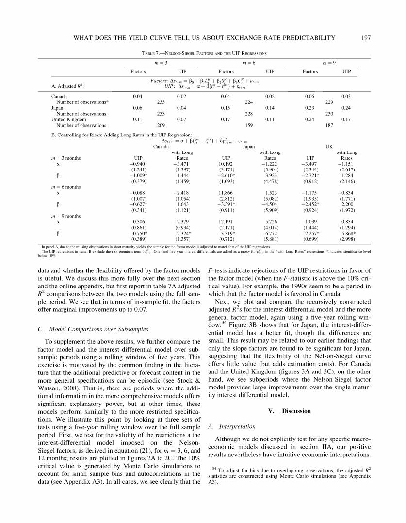
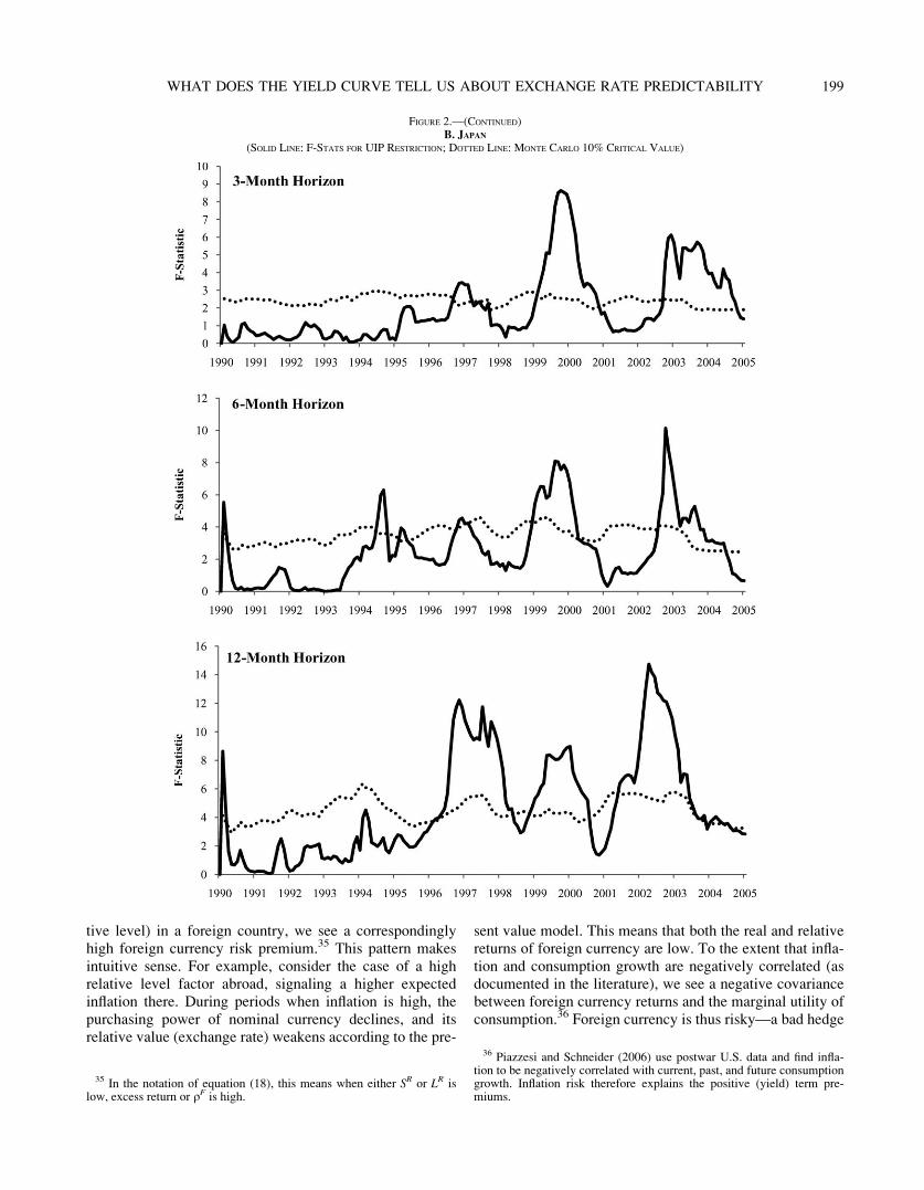
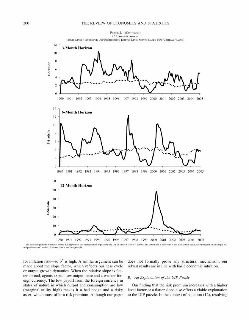
To supplement the above results, we further compare thefactor model and the interest differential model over sub-sample periods using a rolling window of five years. Thisexercise is motivated by the common finding in the litera-ture that the additional predictive or forecast content in themore general specifications can be episodic (see Stock &Watson, 2008). That is, there are periods where the addi-tional information in the more comprehensive models offerssignificant explanatory power, but at other times, thesemodels perform similarly to the more restricted specifica-tions. We illustrate this point by looking at three sets oftests using a five-year rolling window over the full sampleperiod. First, we test for the validity of the restrictions a theinterest-differential model imposed on the Nelson-Siegel factors, as derived in equation (21), for m ¼ 3, 6, and12 months; results are plotted in figures 2A to 2C. The 10%critical value is generated by Monte Carlo simulations toaccount for small sample bias and autocorrelations in thedata (see Appendix A3). In all cases, we see clearly that the

F-tests indicate rejections of the UIP restrictions in favor ofthe factor model (when the F-statistic is above the 10% cri-tical value). For example, the 1990s seem to be a period inwhich that the factor model is favored in Canada.

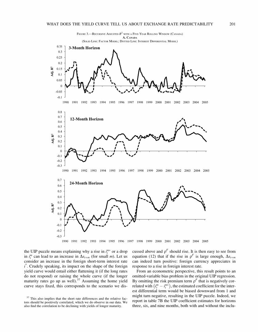
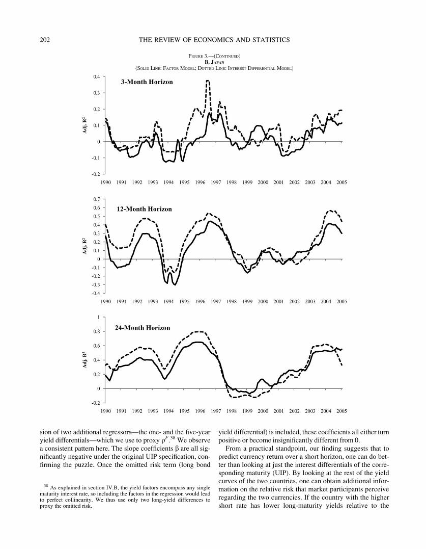
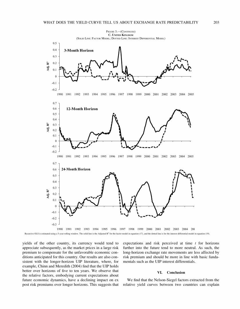
Next, we plot and compare the recursively constructedadjusted R2s for the interest differential model and the moregeneral factor model, again using a five-year rolling win-dow.34 Figure 3B shows that for Japan, the interest-differ-ential model has a better fit, though the differences aresmall. This result may be related to our earlier findings thatonly the slope factors are found to be significant for Japan,suggesting that the flexibility of the Nelson-Siegel curveoffers little value (but adds estimation costs). For Canadaand the United Kingdom (figures 3A and 3C), on the otherhand, we see subperiods where the Nelson-Siegel factormodel provides large improvements over the single-matur-ity interest differential model.

V. Discussion

A. Interpretation

Although we do not explicitly test for any specific macro-economic models discussed in section IIA, our positiveresults nevertheless have intuitive economic interpretations.

TABLE 7.—NELSON-SIEGEL FACTORS AND THE UIP REGRESSIONS

m ¼ 3 m ¼ 6 m ¼ 9

Factors UIP Factors UIP Factors UIP

Factors : Dstþm ¼ b0 þ b1LRt þ b2SR

t þ b3CRt þ utþm

A. Adjusted R2: UIP : Dstþm ¼ aþ b imt � im�

t

� �þ etþm

Canada 0.04 0.02 0.04 0.02 0.06 0.03Number of observations* 233 224 229

Japan 0.06 0.04 0.15 0.14 0.23 0.24Number of observations 233 228 230

United Kingdom 0.11 0.07 0.17 0.11 0.24 0.17Number of observations 209 159 187

B. Controlling for Risks: Adding Long Rates in the UIP Regression:Dstþm ¼ aþ b imt � im�t

� �þ dqF

tþm þ etþm

Canada Japan UK

m ¼ 3 months UIPwith Long

Rates UIPwith Long

Rates UIPwith Long

Ratesa �0.940 �3.471 10.192 �1.222 �3.497 �1.151

(1.241) (1.397) (3.171) (5.904) (2.344) (2.617)b �1.009* 1.444 �2.610* 3.923 �2.721* 1.284

(0.379) (1.459) (1.093) (4.478) (0.912) (2.146)m ¼ 6 months

a �0.088 �2.418 11.866 1.523 �1.175 �0.834(1.007) (1.054) (2.812) (5.082) (1.935) (1.771)

b �0.627* 1.643 �3.391* �4.504 �2.452* 2.200(0.341) (1.121) (0.911) (5.909) (0.924) (1.972)

m ¼ 9 monthsa �0.306 �2.379 12.191 5.726 �1.039 �0.834

(0.861) (0.934) (2.171) (4.014) (1.444) (1.294)b �0.750* 2.324* �3.319* �6.772 �2.257* 5.868*

(0.389) (1.357) (0.712) (5.881) (0.699) (2.998)

In panel A, due to the missing observations in short maturity yields, the sample for the factor model is adjusted to match that of the UIP regressions.The UIP regressions in panel B exclude the risk premium term dqF

tþm . One- and five-year interest differentials are added as a proxy for qFtþm in the ‘‘with Long Rates’’ regressions. *Indicates significance level

below 10%.

34 To adjust for bias due to overlapping observations, the adjusted-R2

statistics are constructed using Monte Carlo simulations (see AppendixA3).


As discussed in section IIB, the yield curve literature showsthat when a country’s yield curve is flat or its level high, themarket expects a forthcoming economic downturn or risinginflation in that country, respectively. Keeping everythingelse equal, our results show that in these situations, its cur-rency is less desirable and faces depreciation pressure, inaccordance with the present value relation, as in equation(8). Subsequently, its currency will appreciate and recovertoward its long-run equilibrium level. Our finding that thereis a declining impact of yield curve information on currency

movements further into the horizon supports this view andsuggests that movements in market expectations tend to betransitory.

Assuming away systematic market expectation errors,excess foreign currency return can be considered the riskpremium associated with holding this currency (see equa-tion [12]). Our results show that the currency risk premium,qF, correlates strongly with the relative yield curve factors.When market expectations point to more output decline(flatter relative slope) or higher future inflation (higher rela-

FIGURE 2.—ROLLING TEST OF THE INTEREST DIFFERENTIAL RESTRICTIONS FOR CANADA, JAPAN, AND THE UNITED KINGDOM

A. CANADA

(SOLID LINE: F-STATS FOR UIP RESTRICTION; DOTTED LINE: MONTE CARLO 10% CRITICAL VALUE)


tive level) in a foreign country, we see a correspondinglyhigh foreign currency risk premium.35 This pattern makesintuitive sense. For example, consider the case of a highrelative level factor abroad, signaling a higher expectedinflation there. During periods when inflation is high, thepurchasing power of nominal currency declines, and itsrelative value (exchange rate) weakens according to the pre-

sent value model. This means that both the real and relativereturns of foreign currency are low. To the extent that infla-tion and consumption growth are negatively correlated (asdocumented in the literature), we see a negative covariancebetween foreign currency returns and the marginal utility ofconsumption.36 Foreign currency is thus risky—a bad hedge



35 In the notation of equation (18), this means when either SR or LR islow, excess return or qF is high.

36 Piazzesi and Schneider (2006) use postwar U.S. data and find infla-tion to be negatively correlated with current, past, and future consumptiongrowth. Inflation risk therefore explains the positive (yield) term pre-miums.


for inflation risk—so qF is high. A similar argument can bemade about the slope factor, which reflects business cycleor output growth dynamics. When the relative slope is flat-ter abroad, agents expect low output there and a weaker for-eign currency. The low payoff from the foreign currency instates of nature in which output and consumption are low(marginal utility high) makes it a bad hedge and a riskyasset, which must offer a risk premium. Although our paper

does not formally prove any structural mechanism, ourrobust results are in line with basic economic intuition.

B. An Explanation of the UIP Puzzle

Our finding that the risk premium increases with a higherlevel factor or a flatter slope also offers a viable explanationto the UIP puzzle. In the context of equation (12), resolving



The solid line plots the F-statistic for the null hypothesis that the restriction imposed by the UIP on the N-S factors is correct. The dotted line is the Monte Carlo 10% critical value, accounting for small sample biasand persistence of the data. For more details, see the appendix.


the UIP puzzle means explaining why a rise in im�t or a drop

in imt can lead to an increase in Dstþm (for small m). Let us

consider an increase in the foreign short-term interest ratei*. Crudely speaking, its impact on the shape of the foreignyield curve would entail either flattening it (if the long ratesdo not respond) or raising the whole curve (if the longermaturity rates go up as well).37 Assuming the home yieldcurve stays fixed, this corresponds to the scenario we dis-

cussed above and qF should rise. It is then easy to see fromequation (12) that if the rise in qF is large enough, Dstþm

can indeed turn positive: foreign currency appreciates inresponse to a rise in foreign interest rate.

From an econometric perspective, this result points to anomitted-variable bias problem in the original UIP regression.By omitting the risk premium term qF that is negatively cor-related with im

t � im�t

� �, the estimated coefficient for the inter-

est differential term would be biased downward from 1 andmight turn negative, resulting in the UIP puzzle. Indeed, wereport in table 7B the UIP coefficient estimates for horizonsthree, six, and nine months, both with and without the inclu-

FIGURE 3.—RECURSIVE ADJUSTED R2WITH A FIVE-YEAR ROLLING WINDOW (CANADA)A. CANADA

(SOLID LINE: FACTOR MODEL; DOTTED LINE: INTEREST DIFFERENTIAL MODEL)

37 This also implies that the short rate differences and the relative fac-tors should be positively correlated, which we do observe in our data. Wealso find the correlation to be declining with yields of longer maturity.


sion of two additional regressors—the one- and the five-yearyield differentials—which we use to proxy qF.38 We observea consistent pattern here. The slope coefficients b are all sig-nificantly negative under the original UIP specification, con-firming the puzzle. Once the omitted risk term (long bond

yield differential) is included, these coefficients all either turnpositive or become insignificantly different from 0.

From a practical standpoint, our finding suggests that topredict currency return over a short horizon, one can do bet-ter than looking at just the interest differentials of the corre-sponding maturity (UIP). By looking at the rest of the yieldcurves of the two countries, one can obtain additional infor-mation on the relative risk that market participants perceiveregarding the two currencies. If the country with the highershort rate has lower long-maturity yields relative to the



38 As explained in section IV.B, the yield factors encompass any singlematurity interest rate, so including the factors in the regression would leadto perfect collinearity. We thus use only two long-yield differences toproxy the omitted risk.


yields of the other country, its currency would tend toappreciate subsequently, as the market prices in a large riskpremium to compensate for the unfavorable economic con-ditions anticipated for this country. Our results are also con-sistent with the longer-horizon UIP literature, where, forexample, Chinn and Meredith (2004) find that the UIP holdsbetter over horizons of five to ten years. We observe thatthe relative factors, embodying current expectations aboutfuture economic dynamics, have a declining impact on expost risk premiums over longer horizons. This suggests that

expectations and risk perceived at time t for horizonsfurther into the future tend to more neutral. As such, thelong-horizon exchange rate movements are less affected byrisk premium and should be more in line with basic funda-mentals such as the UIP interest differentials.

VI. Conclusion

We find that the Nelson-Siegel factors extracted from therelative yield curves between two countries can explain



Recursive OLS is estimated using a 5-year rolling window. The solid line is the Adjusted R2 for the factor model in equation (17), and the dotted line is for the interest differential model in equation (19).


future exchange rate movements and excess currencyreturns. Unlike the exchange rate disconnect conclusion thathas dominated the literature, our results provide support forthe view that exchange rate movements are systematicallyrelated to expected future macroeconomic fundamentals inaccordance with theoretical models that imply a presentvalue relationship. The main insight here is that since mar-ket expectations may be too complicated to be captured bysimple statistical models, we should look for such informa-tion in the data. Given that the term structure of interestrates has been found to embody market expectations offuture macroeconomic dynamics, the present valueexchange rate models can thus be tested without having toimpose either structural or statistical assumptions on theexpectation-formation process. Our findings support thisapproach: the difference between two countries’ yieldcurves can predict the relative value of their currencies andrisk premiums. Our results also, as a natural consequence,offer a simple and intuitive explanation for the UIP puzzle.

REFERENCES

Ang, Andrew, Monika Piazzesi, and Min Wei, ‘‘What Does the YieldCurve Tell us about GDP Growth?’’ Journal of Econometrics 131(2006), 359–403.

Barr, David G., and John Y. Campbell, ‘‘Inflation, Real Interest Rates,and the Bond Market: A Study of UK Nominal and Index-LinkedGovernment Bond Prices,’’ Journal of Monetary Economics 39(1997), 361–383.

Bekaert, Geert, Seonghoon Cho, and Antonio Moreno, ‘‘New-KeynesianMacroeconomics and the Term Structure,’’ Journal of Money,Credit and Banking 42 (2010), 33–62.

Bekaert, Geert, Min Wei, and Yuhang Xing, ‘‘Uncovered Interest RateParity and the Term Structure,’’ Journal of International Moneyand Finance 26 (2007), 1038–1069.

Boudoukh, J., M. P. Richardson, and R. F. Whitelaw, ‘‘The Informationin Long-Maturity Forward Rates: Implications for Exchange Ratesand the Forward Premium Anomaly,’’ NBER working paper11840 (2005).

Chen, Yu-chin, and Kenneth S. Rogoff, ‘‘Commodity Currencies,’’ Jour-nal of International Economics 60, (2003), 133–160.

Chen, Yu-chin, and Kwok Ping Tsang, ‘‘Risk versus Expectations inExchange Rates: A Macro-Finance Approach,’’ University ofWashington working paper (2009).

Chen, Yu-chin, Kwok Ping Tsang, and Wen Jen Tsay, ‘‘Home Bias inCurrency Forecast,’’ University of Washington working paper(2010).

Chinn, Menzie, ‘‘The (Partial) Rehabilitation of Interest Rate Parity: LongerHorizons, Alternative Expectations and Emerging Markets,’’ Journalof International Money and Finance 25 (2006), 7–21.

Chinn, Menzie, and Guy Meredith, ‘‘Long-Horizon Uncovered InterestRate Parity,’’ IMF staff paper, 51:3 (2004).

Clarida, Richard H., Lucio Sarno, Mark P. Taylor, and Giorgio Valente,‘‘The Out-of-Sample Success of Term Structure Models asExchange Rate Predictors: A Step Beyond,’’ Journal of Interna-tional Economics 60 (2003), 61–83.

Clarida, Richard H., and Mark P. Taylor, ‘‘The Term Structure of For-ward Exchange Premiums and the Forecastability of SpotExchange Rates: Correcting the Errors,’’ this REVIEW 79 (1997),353–361.

Clarida, Richard, and Daniel Waldman, ‘‘Is Bad News about InflationGood News for the Exchange Rate?’’ in John Y. Campbell (ed.),Asset Prices and Monetary Policy (Chicago: University of ChicagoPress, 2008).

de los Rios, Antonio Diez, ‘‘Can Affine Term Structure Models Help UsPredict Exchange Rates?’’ Journal of Money, Credit and Banking41 (2009), 755–766.

Dewachter, Hans, and Macro Lyrio, ‘‘Macro Factors and the Term Struc-ture of Interest Rates,’’ Journal of Money, Credit and Banking 38(2006), 119–140.

Diebold, Francis X., C. Li, and Vivian Yue, ‘‘Global Yield Curve Dynamicsand Interactions: A Generalized Nelson-Siegel Approach,’’ Journalof Econometrics 146 (2008), 351–363.

Diebold, F. X., M. Piazzesi, and G. D. Rudebusch, ‘‘Modeling BondYields in Finance and Macroeconomics,’’ American EconomicReview 95 (2005), 415–420.

Diebold, F. X., G. D. Rudebusch, and B. Aruoba, ‘‘The Macroeconomyand the Yield Curve: A Dynamic Latent Factor Approach,’’ Jour-nal of Econometrics 131 (2006), 309–338.

Dornbusch, Rudiger, ‘‘Expectations and Exchange Rate Dynamics,’’Journal of Political Economy 84 (1976), 1161–1176.

Duffee, G. R., ‘‘Term Premia and Interest Rate Forecasts in Affine Mod-els,’’ Journal of Finance 57 (2002), 405–443.

Eichenbaum, Martin, and Charles L. Evans, ‘‘Some Empirical Evidenceon the Effects of Shocks to Monetary Policy on Exchange Rates,’’Quarterly Journal of Economics 100 (1995), 975–1009.

Elliott, G., T. J. Rothenberg, & J. H. Stock, ‘‘Efficient Tests for an Auto-regressive Unit Root,’’ Econometrica 64 (1996) 813–836.

Engel, Charles, ‘‘The Forward Discount Anomaly and the Risk Premium:A Survey of Recent Evidence,’’ Journal of Empirical Finance 3(1996), 123–192.

Engel, Charles, and Kenneth D. West, ‘‘Exchange Rates and Fundamen-tals,’’ Journal of Political Economy 113 (2005), 485–517.

Estrella, Arturo, ‘‘Why Does the Yield Curve Predict Output and Infla-tion?’’ Economic Journal 115 (2005), 722–744.

Estrella, Arturo, and Frederic S. Mishkin, ‘‘Predicting U.S. Recessions:Financial Variables as Leading Indicators,’’ this REVIEW 80 (1998),45–61.

Fama, Eugene F., ‘‘Forward and Spot Exchange Rates,’’ Journal of Mone-tary Economics 14 (1984), 319–338.

Fama, Eugene, and Robert R. Bliss, ‘‘The Information in Long-MaturityForward Rates,’’ American Economic Review 77 (1987), 680–692.

Frankel, Jeffery, ‘‘On the Mark: A Theory of Floating Exchange RatesBased on Real Interest Differentials,’’ American Economic Review69 (1979), 610–623.

Frankel, Jeffery, and Andrew Rose, ‘‘Empirical Research on NominalExchange Rates’’ (pp. 1689–1729), in Gene Grossman and Ken-neth Rogoff (eds.), Handbook of International Economics, vol. 3,(Amsterdam: Elsevier Science, 1995).

Froot, Kenneth, and Jeffrey Frankel, ‘‘Forward Discount Bias: Is It anExchange Risk Premium?’’ Quarterly Journal of Economics 104(1989), 139–161.

Gourinchas, Pierre-Olivier, and Aaron Tornell, ‘‘Exchange Rate Puzzlesand Distorted Beliefs,’’ Journal of International Economics 64(2004), 303–333.

Hamilton, James D., and Dong Heon Kim, ‘‘A Reexamination of the Pre-dictability of Economic Activity Using the Yield Spread,’’ Journalof Money, Credit and Banking 34 (2002), 340–360.

Inci, Ahmet Can, and Biao, Lu, ‘‘Exchange Rates and Interest Rates: CanTerm Structure Models Explain Currency Movements?’’ Journalof Economic Dynamics and Control 28 (2004), 1595–1624.

Krippner, Leo, ‘‘A Yield Curve Perspective on Uncovered Interest Par-ity,’’ University of Waikato, Department of Economics workingpaper (2006).

Mark, Nelson C., ‘‘Exchange Rates and Fundamentals: Evidence onLong-Horizon Predictability,’’ American Economic Review 85(1995), 201–218.

Meese, R., and Kenneth S. Rogoff, ‘‘Empirical Exchange Rate Models ofthe Seventies: Do They Fit Out of Sample?’’ Journal of Interna-tional Economics 14 (1983), 3–24.

Mishkin, Frederic, ‘‘What Does the Term Structure Tell Us about FutureInflation?’’ Journal of Monetary Economics 25 (1990a), 77–95.

——— ‘‘The Information in the Longer Maturity Term Structure aboutFuture Inflation,’’ Quarterly Journal of Economics 105 (1990b),815–828.

Molodtsova, Tanya, Alex Nikolsko-Rzhevskyy, and David H. Papell, ‘‘TaylorRules with Real-Time Data: A Tale of Two Countries and OneExchange Rate,’’ Journal of Monetary Economics 55 (2008), 63–79.

Molodtsova, Tanya, and David H. Papell, ‘‘Out-of-Sample Exchange RatePredictability with Taylor Rule Fundamentals,’’ mimeograph, Uni-versity of Houston (2008).


Moon, Roger, Antonio Rubia, and Rossen Valkanov, ‘‘Long-HorizonRegressions When the Predictor Is Slowly Varying,’’ University ofCalifornia, San Diego working paper (2004).

Mussa, Michael, ‘‘The Exchange Rate, the Balance of Payments,and Monetary and Fiscal Policy under a Regime of ControlledFloating,’’ Scandinavian Journal of Economics 78 (1976), 229–248.

Nelson, Charles R., and Andrew F. Siegel, ‘‘Parsimonious Modeling ofYield Curves,’’ Journal of Business 60 (1987), 473–489.

Pagan, Adrian, ‘‘Econometric Issues in the Analysis of Regressions withGenerated Regressors,’’ International Economic Review 25 (1984),221–247.

Piazzesi, Monika, and Martin Schneider, ‘‘Equilibrium Yield Curves,’’NBER Macro Annual 21 (2006), 389–442.

Rogoff, Kenneth S., and Vania Stavrakeva, ‘‘The Continuing Puzzle ofShort Horizon Exchange Rate Forecasting,’’ NBER working paper14071 (2008).

Rudebusch, Glenn D., and Tao Wu, ‘‘Accounting for a Shift in TermStructure Behavior with No-Arbitrage and Macro-Finance Mod-els,’’ Journal of Money, Credit and Banking 39 (2007), 395–422.

——— ‘‘A Macro-Finance Model of the Term Structure, Monetary Pol-icy and the Economy,’’ Economic Journal 118 (2008), 906–926.

Sarno, Lucio, ‘‘Viewpoint: Towards a Solution to the Puzzles inExchange Rate Economics: Where Do We Stand?’’ CanadianJournal of Economics 38 (2005), 673–708.

Stock, James H., and Mark W. Watson, ‘‘Phillips Curve Inflation Fore-casts,’’ Conference Series [Proceedings], Federal Reserve Bank ofBoston (2008).

Thornton, Daniel L., ‘‘Tests of the Expectations Hypothesis: Resolvingthe Campbell-Shiller Paradox,’’ Journal of Money, Credit andBanking 38 (2006), 511–542.

Valkanov, Rossen, ‘‘Long-Horizon Regressions: Theoretical Results andApplications,’’ Journal of Financial Economics 68 (2003), 201–232.

Wang, Jian, and Jason J. Wu, ‘‘The Taylor Rule and Forecast Intervals forExchange Rates,’’ FRB International Finance discussion paper 963(2009).

Wu, Shu, ‘‘Interest Rate Risk and the Forward Premium Anomaly in For-eign Exchange Markets,’’ Journal of Money, Credit and Banking39 (2007), 423–442.


Documents

Yu-chin Chen and Kwok Ping Tsang* - vtechworks.lib.vt.edu · WHAT DOES THE YIELD CURVE TELL US ABOUT EXCHANGE RATE PREDICTABILITY? Yu-chin Chen and Kwok Ping Tsang* Abstract—Since