Embed Size (px)
Citation preview

Programming Skills inPhysics
Module PH2401
by Dennis Dunn
Version date: Tuesday, 30 October 2007 at 11:11
ComputationalPhysics–Com
putationalPhysics
ComputationalPhysics–Com
putationalPhysics
ComputationalPhysic
s–
ComputationalPhysics
Com
puta
tiona
lPhy
sics–
ComputationalPhysics
Com
puta
tiona
lPhy
sics
–
ComputationalPhysics
Com
puta
tiona
l Phy
sics
–
ComputationalPhysics
Com
puta
tiona
l Phy
sics–
ComputationalPhysics
Computational Physic
s–
Compu
tation
alPhy
sics
Computational Physics– Com
puta
tiona
lPhy
sics
Computational Physics– Com
puta
tiona
lPhy
sics
Computational Physics– Com
puta
tiona
l Phy
sics
Computational Physics–
Compu
tation
alPhy
sics
Computational Physics–
Computational Physics
Com
putational Physics–
Computational Physics
Com
putationalPhysics–
Computational Physics
ComputationalPhysics–
Computational Physics
ComputationalPhysics–
Computational Physics
ComputationalPhysics–Com
putational Physics

2
Copyright c©2003 Dennis Dunn.
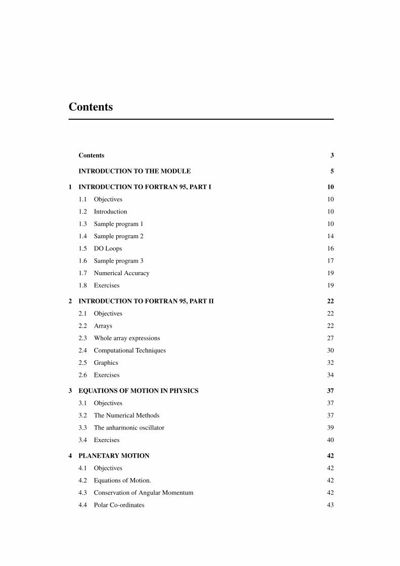
Contents
Contents 3
INTRODUCTION TO THE MODULE 5
1 INTRODUCTION TO FORTRAN 95, PART I 10
1.1 Objectives 10
1.2 Introduction 10
1.3 Sample program 1 10
1.4 Sample program 2 14
1.5 DO Loops 16
1.6 Sample program 3 17
1.7 Numerical Accuracy 19
1.8 Exercises 19
2 INTRODUCTION TO FORTRAN 95, PART II 22
2.1 Objectives 22
2.2 Arrays 22
2.3 Whole array expressions 27
2.4 Computational Techniques 30
2.5 Graphics 32
2.6 Exercises 34
3 EQUATIONS OF MOTION IN PHYSICS 37
3.1 Objectives 37
3.2 The Numerical Methods 37
3.3 The anharmonic oscillator 39
3.4 Exercises 40
4 PLANETARY MOTION 42
4.1 Objectives 42
4.2 Equations of Motion. 42
4.3 Conservation of Angular Momentum 42
4.4 Polar Co-ordinates 43

4
4.5 Numerical solution of equations of motion 44
4.6 Energy and Angular Momentum 44
4.7 Units 45
4.8 Initial Values 45
4.9 The Programme 46
4.10 Kepler’s Laws 47
4.11 Exercises 48
Index 50
INTRODUCTION TO THE MODULE
Version date: Thursday, 30 August, 2007 at 11:40
Introduction
In this module you will be taught techniques employed in computational science and, in particular,computational physics using the FORTRAN95 language. The unit consists of four ‘computer exper-iments’, each of which must be completed within a specified time. Each ‘computer experiment’ isdescribed in a separate chapter of this manual and contains a series of exercises for you to complete.You should work alone and should keep a detailed record of the work in a logbook that must besubmitted for assessment at the end of each experiment.
For three of the four projects, there will be a supervised laboratory session each week and furtherunsupervised sessions.
There will be no supervised sessions for the fourth project: This will be an exercise in independentlearning.
The Salford Fortran95 compiler will be used in this course, and this may be started by double-clicking on the Plato icon under the “Programming - Salford Fortran 95” program group. A “FTN95Help” facility is supplied with this software and can be found within the same program group.This help facility includes details of the standard FORTRAN95 commands as well as the compiler-specific graphics features. All of the programs needed during this course may be downloaded fromthe Part 2 - PH2401 Programming Skills page on the department’s web-server:
(www.rdg.ac.uk/physicsnet).
Web Site Information
In addition to all the chapters and programs required for this course, there are links to other usefulsites including a description of programming style; a description of computational science in generaland FORTRAN programming in particular; a tutorial for FORTRAN90; and a description of object-oriented programming.
References
Programming in Fortran 90/95
By J S Morgan and J L Schonfelder
Published by N.A. Software 2002. 316 pages.
This can be ordered online from
www.fortran.com $15
5
6
Fortran 95 Handbook
By Jeanne Adams, Walt Brainerd, Jeanne Martin, Brian Smith, and Jerry Wagener
Published by MIT Press, 1997. 710 pages.
$55.00
Fortran 95/2003 Explained
By Michael Metcalf and John Reid
Oxford University Press ISBN 0-19-8526293-8
$35.00
Fortran 90 for Scientists and Engineers
By Brian Hahn
Published by Arnold £19.99
Fortran 90/95 for Scientists and Engineers
By Stephen J. Chapman
McGraw-Hill, 1998 ISBN 0-07-011938-4
$68.00
Numerical Recipes in Fortran90
By William Press, Saul Teukolsky, William Vetterling, and Brian FlanneryPublished by Cambridge University Press, 1996. 550 pages. $49.00
A more complete list of reference texts is held at
http://www.fortran.com/fortran/Books/books.html
where books can be ordered directly.
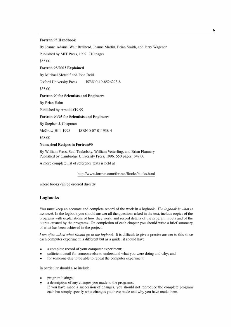
Logbooks
You must keep an accurate and complete record of the work in a logbook. The logbook is what isassessed. In the logbook you should answer all the questions asked in the text, include copies of theprograms with explanations of how they work, and record details of the program inputs and of theoutput created by the programs. On completion of each chapter you should write a brief summaryof what has been achieved in the project.
I am often asked what should go in the logbook. It is difficult to give a precise answer to this sinceeach computer experiment is different but as a guide: it should have
• a complete record of your computer experiment;• sufficient detail for someone else to understand what you were doing and why; and• for someone else to be able to repeat the computer experiment.
In particular should also include:
• program listings;• a description of any changes you made to the programs;
If you have made a succession of changes, you should not reproduce the complete programeach but simply specify what changes you have made and why you have made them.
7
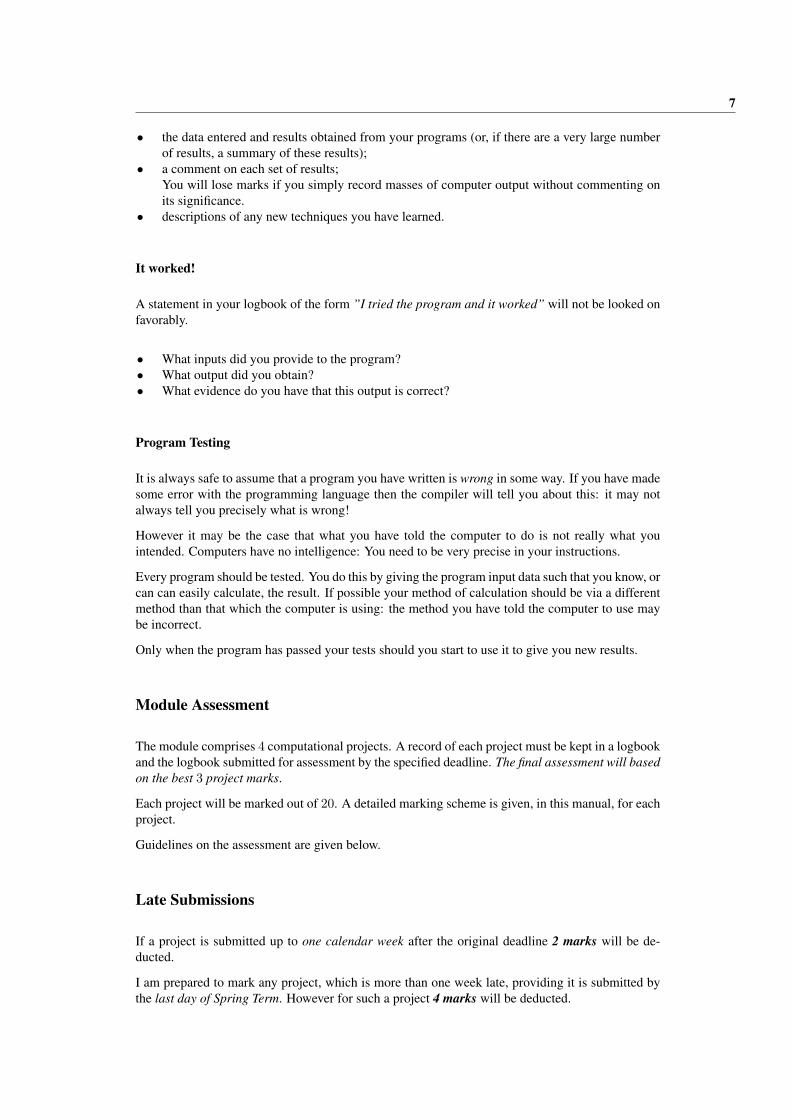
• the data entered and results obtained from your programs (or, if there are a very large numberof results, a summary of these results);
• a comment on each set of results;You will lose marks if you simply record masses of computer output without commenting onits significance.
• descriptions of any new techniques you have learned.
It worked!
A statement in your logbook of the form ”I tried the program and it worked” will not be looked onfavorably.
• What inputs did you provide to the program?• What output did you obtain?• What evidence do you have that this output is correct?
Program Testing
It is always safe to assume that a program you have written is wrong in some way. If you have madesome error with the programming language then the compiler will tell you about this: it may notalways tell you precisely what is wrong!
However it may be the case that what you have told the computer to do is not really what youintended. Computers have no intelligence: You need to be very precise in your instructions.
Every program should be tested. You do this by giving the program input data such that you know, orcan can easily calculate, the result. If possible your method of calculation should be via a differentmethod than that which the computer is using: the method you have told the computer to use maybe incorrect.
Only when the program has passed your tests should you start to use it to give you new results.
Module Assessment
The module comprises 4 computational projects. A record of each project must be kept in a logbookand the logbook submitted for assessment by the specified deadline. The final assessment will basedon the best 3 project marks.
Each project will be marked out of 20. A detailed marking scheme is given, in this manual, for eachproject.
Guidelines on the assessment are given below.
Late Submissions
If a project is submitted up to one calendar week after the original deadline 2 marks will be de-ducted.
I am prepared to mark any project, which is more than one week late, providing it is submitted bythe last day of Spring Term. However for such a project 4 marks will be deducted.
8
Extensions & Extenuating Circumstances
If you have a valid reason for not being able to complete a project by the specified deadline thenyou should
• inform the lecturer as soon as possible; and• complete an Extension of Deadlines Form. The form can be obtained from the School Office
(Physics 210).
If you believe that there has been some non-academic problem that you encountered during themodule (medical or family problems for example) you should complete an Extenuating Circum-stances Form, again obtainable from the School Office, so that the Director of Teaching & Learningand the Examiners can consider this.
Feedback
In addition to comments written in your logbook by the assessor during marking, feedback on theprojects will be provided by a class discussion and, when appropriate, by individual discussion withthe lecturer.
There will be no feedback, apart from the mark, on late submissions.
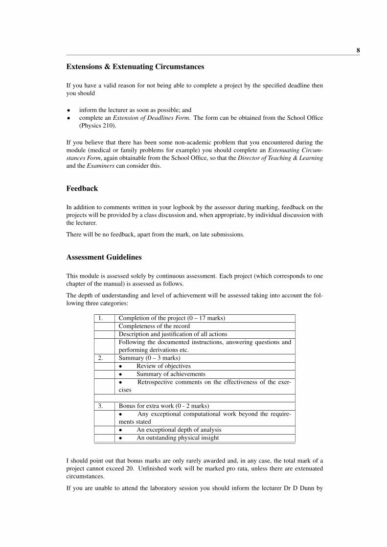
Assessment Guidelines
This module is assessed solely by continuous assessment. Each project (which corresponds to onechapter of the manual) is assessed as follows.
The depth of understanding and level of achievement will be assessed taking into account the fol-lowing three categories:
1. Completion of the project (0 – 17 marks)Completeness of the recordDescription and justification of all actionsFollowing the documented instructions, answering questions andperforming derivations etc.
2. Summary (0 – 3 marks)• Review of objectives• Summary of achievements• Retrospective comments on the effectiveness of the exer-cises
3. Bonus for extra work (0 - 2 marks)• Any exceptional computational work beyond the require-ments stated• An exceptional depth of analysis• An outstanding physical insight
I should point out that bonus marks are only rarely awarded and, in any case, the total mark of aproject cannot exceed 20. Unfinished work will be marked pro rata, unless there are extenuatedcircumstances.
If you are unable to attend the laboratory session you should inform the lecturer Dr D Dunn by

9
telephone 0118 378 8538 or by email [email protected]
Plagiarism
In any learning process you should make use of whatever resources are available. In this course,I hope, the lecturer and postgraduate assistant should be valuable resources. Your fellow studentsmay also be useful resources and I encourage you to discuss the projects with them.
However at the end of these discussions you should then write your own program (or programmodification). It is completely unacceptable to copy someone else’s program (or results). This is aform of cheating and will be dealt with as such.
I should point out that such copying (even if slightly disguised) is very easy to detect.
Time Management
There is ample time for you to complete each of these projects providing you manage your timesensibly.
You should aim to spend at least six hours per week on each project: that is a total of about 18 hoursper project.
Each project is divided into a number of ’exercises’ and each of these exercises is allocated a mark.This mark is approximately proportional to the time that I expect you to spend on the exercise. Youshould therefore be able to allocate your time accordingly: It is not sensible to spend half of theavailable time on an exercise which is worth only a quarter of the total marks.
Each of the projects below is given a deadline. You should not take this as a target. You should setyourself a target well before the deadline.
Projects
• Introduction to Fortran 95 ; Part 1 [Deadline: noon, Wednesday Week 3 Autumn Term]• Introduction to Fortran 95 ; Part 2 [Deadline: noon, Wednesday Week 6 Autumn Term ]• Equations of motion in physics [Deadline: noon, Wednesday Week 9 Autumn Term ]• Planetary motion [Deadline: noon, Wednesday Week 2 Spring Term ]
The ’Planetary motion’ project will be unsupervised and is an exercise in independent learning.Nevertheless the lecturer and demonstrator will be available for consultation.

Chapter 1
INTRODUCTION TO FORTRAN 95, PART I
Version date: Friday, 28 September, 2007 at 13:39
1.1 Objectives
To introduce the basic elements of FORTRAN 95, such as procedures and control structures, throughsample programs and their descriptions. At the end of this chapter students should be able to writeelementary programs and run them using the Salford compiler software.
1.2 Introduction
For nearly fifty years FORTRAN has been the principal language of computational science. It wasintroduced by IBM in the 1950’s and called FORmula TRANslation and it transformed computing.As its name implies it was specifically designed for numerical tasks encountered in the physical andmathematical sciences, and the computational efficiency of the language makes it the language ofchoice for the majority of practicing physicists.
It has evolved over the years and the stages of evolution have been marked by various languagestandards: FORTRAN66 (in about 1966); FORTRAN77 (in about 1977); FORTRAN90 (in 1990);and FORTRAN95 (in 1995). The current version is called FORTRAN2003 but we don’t yet have acompiler which includes the new features for this version.
FORTRAN95 is currently regarded as the best language for most aspects of computational science,object oriented programming being the only area where it is not considered the best. For details seea report by the Computational Science Education Project ‘Fortran and computational science’ onwebsite http://www.phy.ornl.gov/csep/CSEP/PL/PL.html.
FORTRAN95 does contain most (but not all) elements of object oriented programming and alsoincludes many features which make it ideal for vector and parallel processors.
In this first chapter we shall consider the basic elements of the language through sample programs,since it is only through its use that one learns the essential tools of programming. As you progressthrough the course you shall encounter further features of the language whilst reinforcing your previ-ous knowledge. However the emphasis of this course is physics and how computational techniquesprovide a versatile tool for investigating physical situations, rather than simply the programminglanguage itself.
1.3 Sample program 1
The first program is an example of translating a mathematical formula. Consider a triangle withsides x, y and z. The area of a triangle is 1
2base × height. If I take y as the base and θ to be the
10

1.3 Sample program 1 11
angle between the sides of length x and y the formula for the area can be written as
Area = 12yh
h = xsin(θ)cos(θ) = x2+y2−z2
2xy
The last part of this formula can be obtained by writing the three sides as vectors x, y and z andusing the relations
z = x− yz • z = x • x + y • y− 2x • y
The following simple program calculates the area of a triangle whose side lengths are entered by theuser. You should note that this is a (deliberately) poorly written program because it does not checkthat that the input data is valid. You will remedy this defect later.
PROGRAM Triangle
! Version Date: Wednesday, 27 September 2006 at 16:26
! This is a (deliberately) badly written program for determining the! area of a triangle given the lengths of the three sides.! You will improve it
IMPLICIT NONEREAL :: a, b, c, Area
CALL WriteDateAndTime(0)
WRITE(*, *) ’ Enter the lengths of the three sides’WRITE(*, *) ’ Check that they make a triangle ! ’READ(*, *) a, b, cArea = Triangle_Area(a, b, c)
WRITE(*,*) ’ Area of triangle is ’, AreaWRITE(*,*) ’ Press ENTER to stop’READ(*,*)STOP
CONTAINS
FUNCTION Triangle_Area(x,y,z)IMPLICIT NONEREAL :: Triangle_AreaREAL, INTENT(IN) :: x,y,zREAL :: theta, heighttheta = ACOS((x**2 + y**2 - z**2)/(2.0*x*y))height = x*SIN(theta)Triangle_Area = 0.5*y*heightRETURN
END FUNCTION Triangle_Area
SUBROUTINE WriteDateAndTime(UnitNumber)! This subroutine should be used in EVERY program to validate any output
INTEGER, INTENT(IN) :: UnitNumberCHARACTER (LEN=10) :: Current_date, Current_time, Current_zoneINTEGER :: d_values(8)CHARACTER (LEN=40) :: Your_Name
CALL date_and_time(Current_date, Current_time, Current_zone, d_values)
Your_Name = "" ! Insert your name between the quotation marks
IF (UnitNumber .EQ. 0) THENWRITE (*, *) ’ Date: ’, Current_date(1:4),’/’, &
Current_date(5:6),’/’,Current_date(7:8)
1.3 Sample program 1 12
WRITE (*, *) ’ Time: ’, Current_time(1:2),’:’, &Current_time(3:4), ’:’, Current_time(5:6)
WRITE (*, *) Your_NameWRITE (*, *) ’ ====================================== ’
ELSEWRITE (UnitNumber, *) ’ Date: ’, Current_date(1:4),’/’, &
Current_date(5:6),’/’,Current_date(7:8)WRITE (UnitNumber, *) ’ Time: ’, Current_time(1:2),’:’, &
Current_time(3:4), ’:’, Current_time(5:6)WRITE (UnitNumber, *) Your_NameWRITE (UnitNumber, *) ’ ====================================== ’
END IF
RETURNEND SUBROUTINE WriteDateAndTime
END PROGRAM Triangle
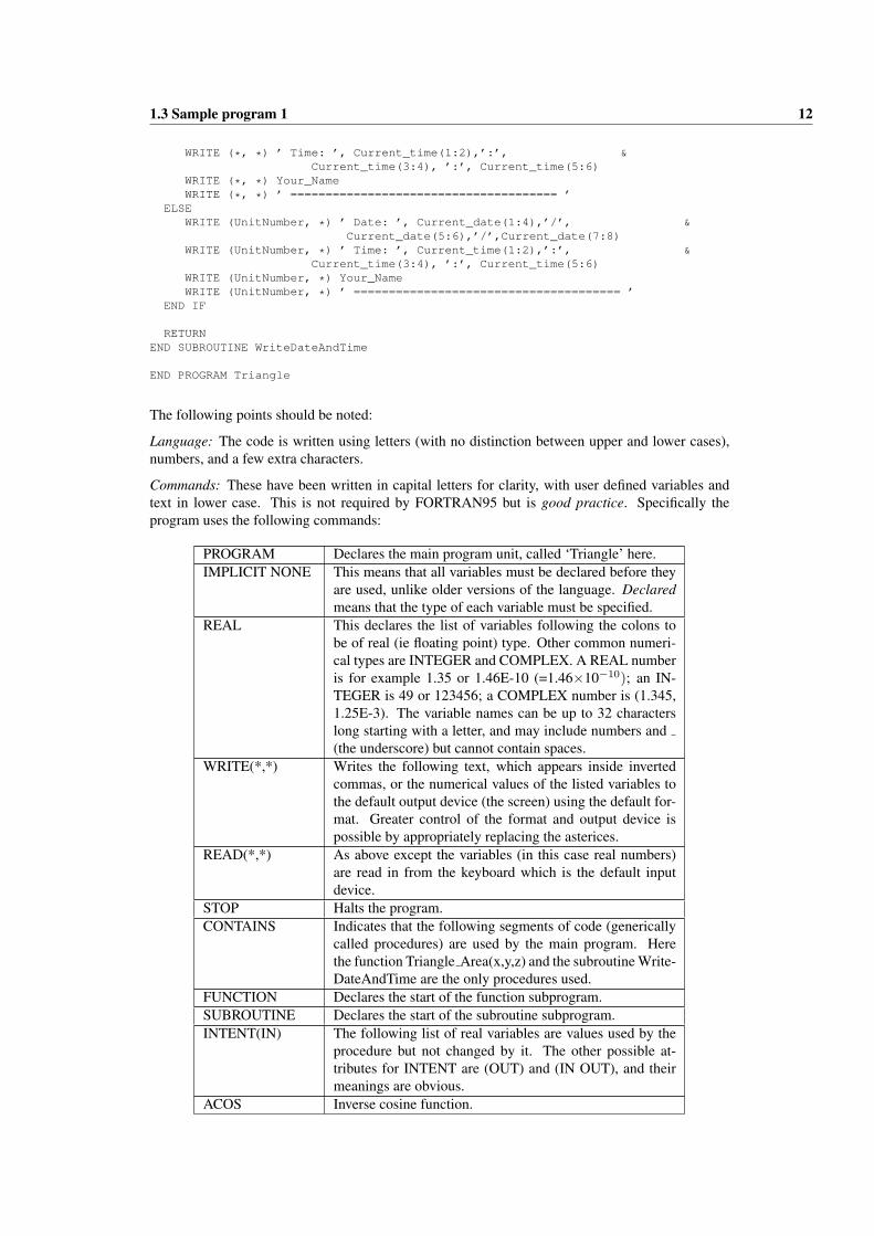
The following points should be noted:
Language: The code is written using letters (with no distinction between upper and lower cases),numbers, and a few extra characters.
Commands: These have been written in capital letters for clarity, with user defined variables andtext in lower case. This is not required by FORTRAN95 but is good practice. Specifically theprogram uses the following commands:
PROGRAM Declares the main program unit, called ‘Triangle’ here.IMPLICIT NONE This means that all variables must be declared before they
are used, unlike older versions of the language. Declaredmeans that the type of each variable must be specified.
REAL This declares the list of variables following the colons tobe of real (ie floating point) type. Other common numeri-cal types are INTEGER and COMPLEX. A REAL numberis for example 1.35 or 1.46E-10 (=1.46×10⁻¹⁰); an IN-TEGER is 49 or 123456; a COMPLEX number is (1.345,1.25E-3). The variable names can be up to 32 characterslong starting with a letter, and may include numbers and(the underscore) but cannot contain spaces.
WRITE(*,*) Writes the following text, which appears inside invertedcommas, or the numerical values of the listed variables tothe default output device (the screen) using the default for-mat. Greater control of the format and output device ispossible by appropriately replacing the asterices.
READ(*,*) As above except the variables (in this case real numbers)are read in from the keyboard which is the default inputdevice.
STOP Halts the program.CONTAINS Indicates that the following segments of code (generically
called procedures) are used by the main program. Herethe function Triangle Area(x,y,z) and the subroutine Write-DateAndTime are the only procedures used.
FUNCTION Declares the start of the function subprogram.SUBROUTINE Declares the start of the subroutine subprogram.INTENT(IN) The following list of real variables are values used by the
procedure but not changed by it. The other possible at-tributes for INTENT are (OUT) and (IN OUT), and theirmeanings are obvious.
ACOS Inverse cosine function.

1.3 Sample program 1 13
SIN Sine function: FORTRAN95 has many built-in mathemat-ical functions.
RETURN Return from the procedure to the main program, at thepoint immediately following the call to the procedure.
END Marks the end of the appropriate program unit.
The WriteDateAndTime subroutine will be used to write out the date and time, and your name eitherto screen or to a disc file. This subroutine will be used in all programs. Don’t try, yet, to understandhow this part of the program works.
You need to edit the WriteDateAndTime subroutine so that the variable Y our Name does containyour name: For example:
Your_Name = ’John Smith’
This subroutine should be used in every program to time-stamp any output and to identify youas the programmer. Any output which is not validated in this way will be discounted.
A complete list of FORTRAN 95 commands is provided in the Salford FTN95 Help (LanguageOverview) program.
Procedures: The use of procedures greatly simplifies programs by making it clearer to a reader howthe program works. It also makes the program easier to check and modify by keeping the block ofcode that performs a specific task packaged in one place.
The procedure used here was the function Triangle Area(x,y,z); ‘function’ means that the variable‘Triangle Area’ itself takes a value. Note the arguments (x, y, z) are dummy variable names; they donot have to be the same names (a, b, c) as those used in the main program that uses the procedure.However they do have to be the same types. Suppose a function func is defined in a functionsubroutine to have variables u, v and w and is used in a program as func(r, s, t) Then r must be ofthe same type as u, s must be of the same type as v and t must be of the same type as w.
This makes procedures very versatile. They can be used several times within the main program, andvery often they have been written elsewhere so that the user does not have to know exactly how theywork and can treat them like ‘black boxes’. Libraries of sophisticated procedures exist that performcommon tasks such as integrating functions, finding eigenvalues of matrices etc.
1.3.1 Capturing computer output
The computer will normally send its output to the screen – you will learn later how to send theoutput to a disc file.
If you want to ’capture’ the screen output so that you can put it into your logbook then:
• first make sure that the screen window you require is ’active’. You do this by ’clicking’ in thewindow.
• Then press the keys [ALT] [Print Screen] simultaneously. This captures the particular windowand stores it in the ’clipboard’.
• Open Word, or something similar, and paste the clipboard into a document. You can then printthis as normal.
1.3.2 = does not mean equals
It is important point to note that = does not simply mean ’equals’. Consider a simple program line
A = B + C
1.4 Sample program 2 14
This is not a mathematical statement saying that A is equal to the sum of B and C but is ratheran operation. This operation adds the current values of the variables B and C and puts the resultinto the variable A. The previous value of variable A has been erased (or over-written in computer-speak).
A verbal statement of the operation is ’make A equal to B + C’.
1.3.3 Testing the program
In order to test this program you should invent some triangles which are simple enough that youcan easily calculate the area. You should not restrict your tests to right-angled triangles: Supposethe program gives the correct results for a right-angled triangle but fails for others. Your calculationshould certainly not use the formula employed by the program: This might be wrong!
If you understand what you have read, you may now attempt the first exercise given at the end ofthis chapter.
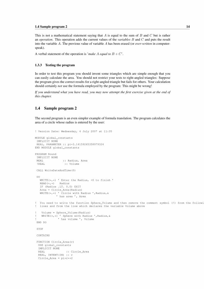
1.4 Sample program 2
The second program is an even simpler example of formula translation. The program calculates thearea of a circle whose radius is entered by the user:
! Version Date: Wednesday, 4 July 2007 at 11:35
MODULE global_constantsIMPLICIT NONEREAL, PARAMETER :: pi=3.14159265358979324END MODULE global_constants
PROGRAM RoundIMPLICIT NONEREAL :: Radius, Area!REAL :: Volume
CALL WriteDateAndTime(0)
DOWRITE(*,*) ’ Enter the Radius, <0 to finish ’READ(*,*) RadiusIF (Radius .LT. 0.0) EXITArea = Circle_Area(Radius)WRITE(*,*) ’ Circle with Radius ’,Radius,&
’ has area ’, Area
! You need to write the function Sphere_Volume and then remove the comment symbol (!) from the following! lines and from the line which declares the variable Volume above
! Volume = Sphere_Volume(Radius)! WRITE(*,*) ’ Sphere with Radius ’,Radius,&! ’ has volume ’, VolumeEND DO
STOP
CONTAINS
FUNCTION Circle_Area(r)USE global_constantsIMPLICIT NONEREAL :: Circle_AreaREAL, INTENT(IN) :: rCircle_Area = pi*r**2
1.4 Sample program 2 15
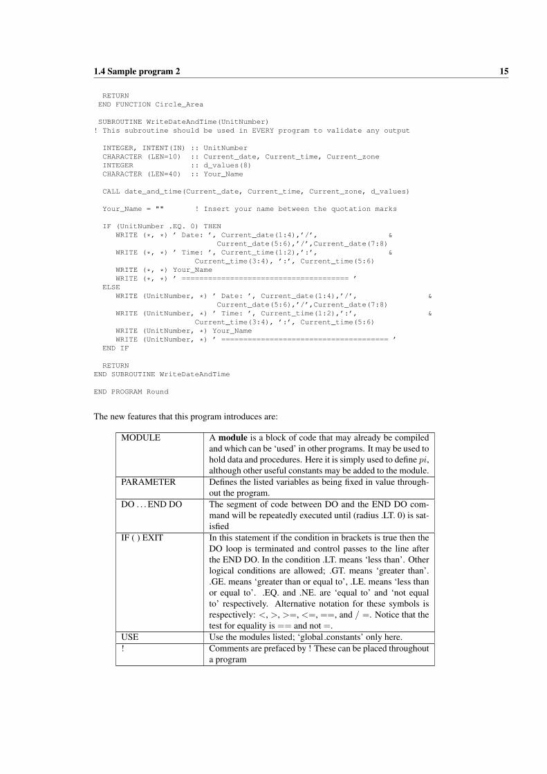
RETURNEND FUNCTION Circle_Area
SUBROUTINE WriteDateAndTime(UnitNumber)! This subroutine should be used in EVERY program to validate any output
INTEGER, INTENT(IN) :: UnitNumberCHARACTER (LEN=10) :: Current_date, Current_time, Current_zoneINTEGER :: d_values(8)CHARACTER (LEN=40) :: Your_Name
CALL date_and_time(Current_date, Current_time, Current_zone, d_values)
Your_Name = "" ! Insert your name between the quotation marks
IF (UnitNumber .EQ. 0) THENWRITE (*, *) ’ Date: ’, Current_date(1:4),’/’, &
Current_date(5:6),’/’,Current_date(7:8)WRITE (*, *) ’ Time: ’, Current_time(1:2),’:’, &
Current_time(3:4), ’:’, Current_time(5:6)WRITE (*, *) Your_NameWRITE (*, *) ’ ====================================== ’
ELSEWRITE (UnitNumber, *) ’ Date: ’, Current_date(1:4),’/’, &
Current_date(5:6),’/’,Current_date(7:8)WRITE (UnitNumber, *) ’ Time: ’, Current_time(1:2),’:’, &
Current_time(3:4), ’:’, Current_time(5:6)WRITE (UnitNumber, *) Your_NameWRITE (UnitNumber, *) ’ ====================================== ’
END IF
RETURNEND SUBROUTINE WriteDateAndTime
END PROGRAM Round
The new features that this program introduces are:
MODULE A module is a block of code that may already be compiledand which can be ‘used’ in other programs. It may be used tohold data and procedures. Here it is simply used to define pi,although other useful constants may be added to the module.
PARAMETER Defines the listed variables as being fixed in value through-out the program.
DO . . . END DO The segment of code between DO and the END DO com-mand will be repeatedly executed until (radius .LT. 0) is sat-isfied
IF ( ) EXIT In this statement if the condition in brackets is true then theDO loop is terminated and control passes to the line afterthe END DO. In the condition .LT. means ‘less than’. Otherlogical conditions are allowed; .GT. means ‘greater than’..GE. means ‘greater than or equal to’, .LE. means ‘less thanor equal to’. .EQ. and .NE. are ‘equal to’ and ‘not equalto’ respectively. Alternative notation for these symbols isrespectively: <, >, >=, <=, ==, and / =. Notice that thetest for equality is == and not =.
USE Use the modules listed; ‘global constants’ only here.! Comments are prefaced by ! These can be placed throughout
a program
1.5 DO Loops 16
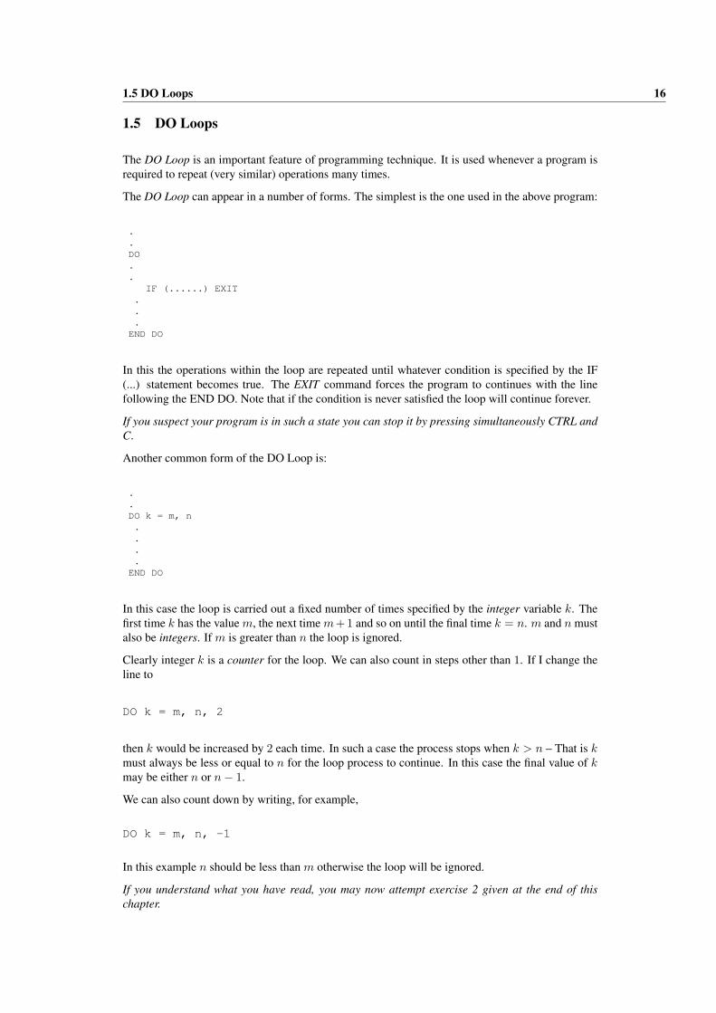
1.5 DO Loops
The DO Loop is an important feature of programming technique. It is used whenever a program isrequired to repeat (very similar) operations many times.
The DO Loop can appear in a number of forms. The simplest is the one used in the above program:
.
.DO..
IF (......) EXIT...END DO
In this the operations within the loop are repeated until whatever condition is specified by the IF(...) statement becomes true. The EXIT command forces the program to continues with the linefollowing the END DO. Note that if the condition is never satisfied the loop will continue forever.
If you suspect your program is in such a state you can stop it by pressing simultaneously CTRL andC.
Another common form of the DO Loop is:
.
.DO k = m, n....END DO
In this case the loop is carried out a fixed number of times specified by the integer variable k. Thefirst time k has the value m, the next time m+1 and so on until the final time k = n. m and n mustalso be integers. If m is greater than n the loop is ignored.
Clearly integer k is a counter for the loop. We can also count in steps other than 1. If I change theline to
DO k = m, n, 2
then k would be increased by 2 each time. In such a case the process stops when k > n – That is kmust always be less or equal to n for the loop process to continue. In this case the final value of kmay be either n or n− 1.
We can also count down by writing, for example,
DO k = m, n, -1
In this example n should be less than m otherwise the loop will be ignored.
If you understand what you have read, you may now attempt exercise 2 given at the end of thischapter.
1.6 Sample program 3 17
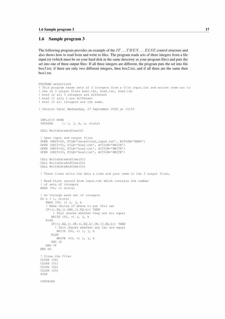
1.6 Sample program 3
The following program provides an example of the IF . . . THEN . . . ELSE control structure andalso shows how to read from and write to files. The program reads sets of three integers from a fileinput.txt (which must be on your hard disk in the same directory as your program files) and puts theset into one of three output files: If all three integers are different, the program puts the set into filebox3.txt; if there are only two different integers, then box2.txt; and if all three are the same thenbox1.txt.
PROGRAM selections! This program reads sets of 3 integers from a file input.txt and writes them out to! one of 3 output files box1.txt, box2.txt, box3.txt! box3 if all 3 integers are different! box2 if only 2 are different! box1 if all integers are the same.
! Version Date: Wednesday, 27 September 2006 at 16:53
IMPLICIT NONEINTEGER :: i, j, k, n, ntotal
CALL WriteDateAndTime(0)
! Open input and output filesOPEN (UNIT=50, FILE=’selections_input.txt’, ACTION=’READ’)OPEN (UNIT=51, FILE=’box1.txt’, ACTION=’WRITE’)OPEN (UNIT=52, FILE=’box2.txt’, ACTION=’WRITE’)OPEN (UNIT=53, FILE=’box3.txt’, ACTION=’WRITE’)
CALL WriteDateAndTime(51)CALL WriteDateAndTime(52)CALL WriteDateAndTime(53)
! These lines write the date & time and your name to the 3 output files.
! Read first record from input.txt which contains the number! of sets of integersREAD (50, *) ntotal
! Go through each set of integersDO n = 1, ntotal
READ (50, *) i, j, k! Make choice of where to put this setIF((i.EQ.j).AND.(i.EQ.k)) THEN
! This checks whether they are all equalWRITE (51, *) i, j, k
ELSEIF((i.EQ.j).OR.(i.EQ.k).OR.(j.EQ.k)) THEN
! This checks whether any two are equalWRITE (52, *) i, j, k
ELSEWRITE (53, *) i, j, k
END IFEND IF
END DO
! Close the filesCLOSE (50)CLOSE (51)CLOSE (52)CLOSE (53)STOP
CONTAINS
1.6 Sample program 3 18
SUBROUTINE WriteDateAndTime(UnitNumber)! This subroutine should be used in EVERY program to validate any output
INTEGER, INTENT(IN) :: UnitNumberCHARACTER (LEN=10) :: Current_date, Current_time, Current_zoneINTEGER :: d_values(8)CHARACTER (LEN=40) :: Your_Name
CALL date_and_time(Current_date, Current_time, Current_zone, d_values)
Your_Name = "" ! Insert your name between the quotation marks
IF (UnitNumber .EQ. 0) THENWRITE (*, *) ’ Date: ’, Current_date(1:4),’/’, &
Current_date(5:6),’/’,Current_date(7:8)WRITE (*, *) ’ Time: ’, Current_time(1:2),’:’, &
Current_time(3:4), ’:’, Current_time(5:6)WRITE (*, *) Your_NameWRITE (*, *) ’ ====================================== ’
ELSEWRITE (UnitNumber, *) ’ Date: ’, Current_date(1:4),’/’, &
Current_date(5:6),’/’,Current_date(7:8)WRITE (UnitNumber, *) ’ Time: ’, Current_time(1:2),’:’, &
Current_time(3:4), ’:’, Current_time(5:6)WRITE (UnitNumber, *) Your_NameWRITE (UnitNumber, *) ’ ====================================== ’
END IF
RETURNEND SUBROUTINE WriteDateAndTime
END PROGRAM selections
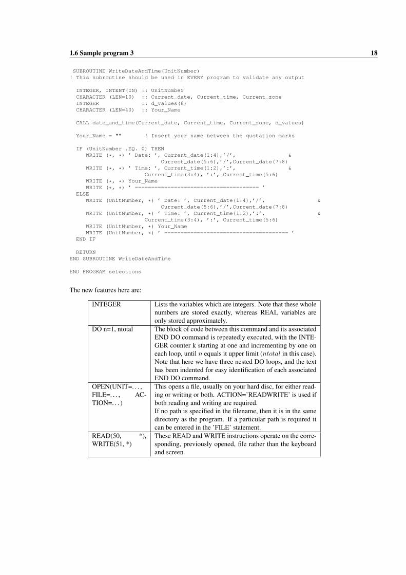
The new features here are:
INTEGER Lists the variables which are integers. Note that these wholenumbers are stored exactly, whereas REAL variables areonly stored approximately.
DO n=1, ntotal The block of code between this command and its associatedEND DO command is repeatedly executed, with the INTE-GER counter k starting at one and incrementing by one oneach loop, until n equals it upper limit (ntotal in this case).Note that here we have three nested DO loops, and the texthas been indented for easy identification of each associatedEND DO command.
OPEN(UNIT=. . . ,FILE=. . . , AC-TION=. . . )
This opens a file, usually on your hard disc, for either read-ing or writing or both. ACTION=’READWRITE’ is used ifboth reading and writing are required.If no path is specified in the filename, then it is in the samedirectory as the program. If a particular path is required itcan be entered in the ’FILE’ statement.
READ(50, *),WRITE(51, *)
These READ and WRITE instructions operate on the corre-sponding, previously opened, file rather than the keyboardand screen.
1.7 Numerical Accuracy 19
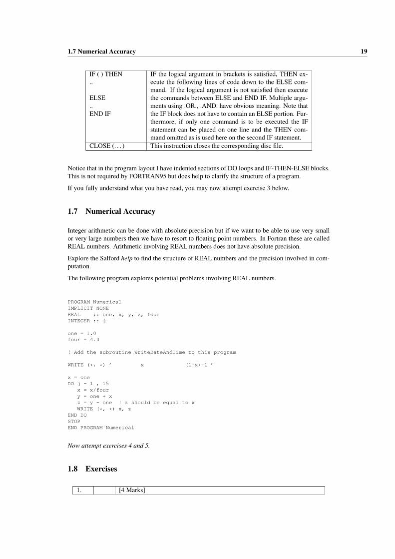
IF ( ) THEN..
ELSE..END IF
IF the logical argument in brackets is satisfied, THEN ex-ecute the following lines of code down to the ELSE com-mand. If the logical argument is not satisfied then executethe commands between ELSE and END IF. Multiple argu-ments using .OR., .AND. have obvious meaning. Note thatthe IF block does not have to contain an ELSE portion. Fur-thermore, if only one command is to be executed the IFstatement can be placed on one line and the THEN com-mand omitted as is used here on the second IF statement.
CLOSE (. . . ) This instruction closes the corresponding disc file.
Notice that in the program layout I have indented sections of DO loops and IF-THEN-ELSE blocks.This is not required by FORTRAN95 but does help to clarify the structure of a program.
If you fully understand what you have read, you may now attempt exercise 3 below.
1.7 Numerical Accuracy
Integer arithmetic can be done with absolute precision but if we want to be able to use very smallor very large numbers then we have to resort to floating point numbers. In Fortran these are calledREAL numbers. Arithmetic involving REAL numbers does not have absolute precision.
Explore the Salford help to find the structure of REAL numbers and the precision involved in com-putation.
The following program explores potential problems involving REAL numbers.
PROGRAM NumericalIMPLICIT NONEREAL :: one, x, y, z, fourINTEGER :: j
one = 1.0four = 4.0
! Add the subroutine WriteDateAndTime to this program
WRITE (*, *) ’ x (1+x)-1 ’
x = oneDO j = 1 , 15
x = x/foury = one + xz = y - one ! z should be equal to xWRITE (*, *) x, z
END DOSTOPEND PROGRAM Numerical
Now attempt exercises 4 and 5.
1.8 Exercises
1. [4 Marks]

1.8 Exercises 20
(a) Obtain a copy of the program Triangle.f95 from the departmental web server.Write down, precisely, the formula for the area of the triangle and identifywhere this is implemented in the program.Start the Salford editor, Plato, and open the Triangle.f95 program. Compilethe program; if any mistakes exist in the program the compiler will reportthe errors to you. If the compilation produces no errors, build the executableprogram and execute it.A window will appear as the program runs. Enter the three side lengths (usesimple right-angled triangles to start with, say 3, 4, 5 or 5, 12, 13) and recordthe value calculated by the program. Check this result analytically.Test the program by entering at least two other (non-right-angled) trianglesfor which you can determine the area.Remember to keep a record of your work in your logbooks.
(b) The area of the triangle should not depend on the order in which youenter the three lengths; Triangle Area(3, 4, 5) should be the same asTriangle Area(4, 5, 3) etc. However the program does the calculations forTriangle Area(3, 4, 5) and Triangle Area(4, 5, 3) in different ways.Save the program under a different name using the ‘Save As’ option under‘File’, and modify it to calculate the area of the triangle using all possiblecombinations of the ordering of the lengths. Do this by calling the func-tion Triangle Area several times with the arguments in different orders egTriangle Area(a, b, c) and Triangle Area(b, a, c)Record the modifications you have made to the program and test it usingseveral sets of sides, including a set in which one side is much smaller thanthe other two.Record the program input and output.
2. [3 Marks](a) Compile and run the program Round.f95 and confirm that it is works cor-
rectly.(b) Make a copy of Round.f95 (Round2.f95, say) and modify it so that the pro-
gram calculates the volume of a sphere as well as the area of the circle withthe given radius. You should do this by creating a new procedure, FUNC-TION Sphere Volume(radius). Take care to incorporate all the necessarycommands; any omissions will be identified by the compiler.One final word of caution; FORTRAN 95 deals with integers precisely, andso division of integers results in rounding down to the nearest integer.Thus 4/3 will result in 1 and 3/4 will result in 0! This is perfectly correct ininteger arithmetic.However if either of the numbers is REAL then a REAL number results:4.0/3 = 4/3.0 = 4.0/3.0 = 1.33333. This situation holds for integer vari-ables as well.
(c) Remember to place a printout of your modified program in your logbook.Explain, in detail, the modifications. Record some sample output producedby the program (together with the corresponding input) and comment brieflyon how the program works.
3. [4 Marks](a) Download the program selections.f95 and the input file selections input.txt.
Compile and run the program Selections.f95, and record the input and outputfiles in your logbook.Explain in your own words how the nested IFs produce the output, and howthe logical IF commands operate in this application.
1.8 Exercises 21
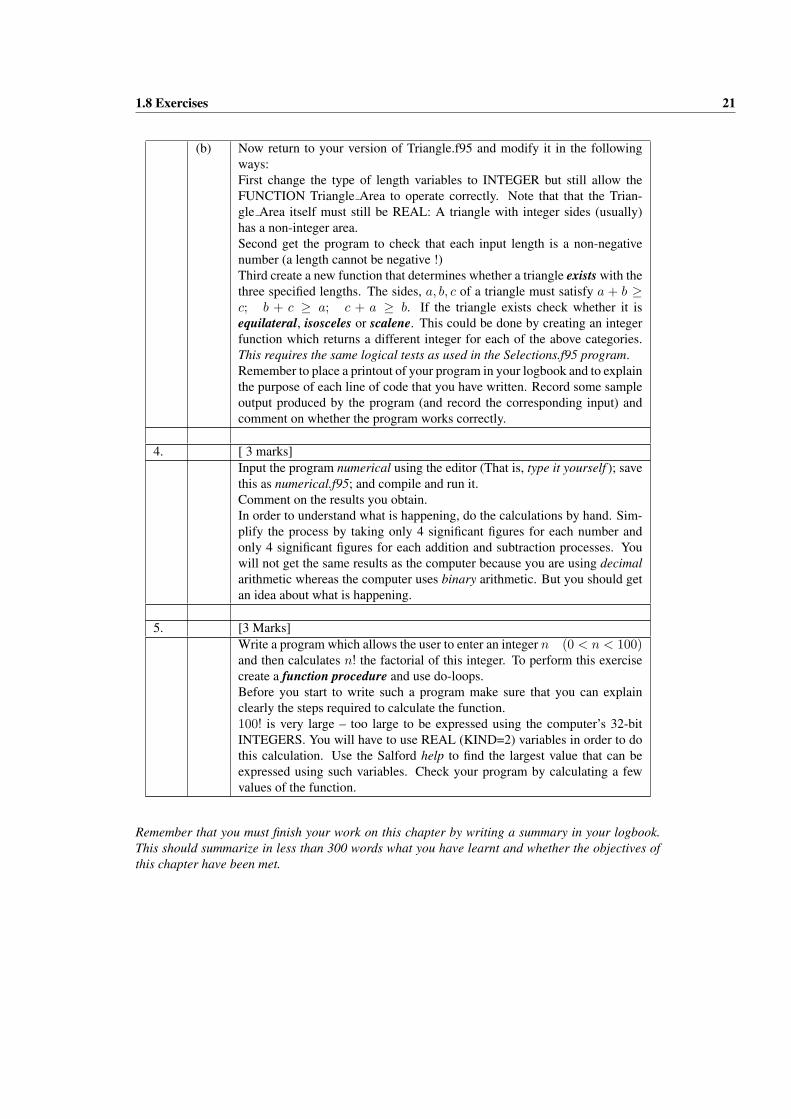
(b) Now return to your version of Triangle.f95 and modify it in the followingways:First change the type of length variables to INTEGER but still allow theFUNCTION Triangle Area to operate correctly. Note that that the Trian-gle Area itself must still be REAL: A triangle with integer sides (usually)has a non-integer area.Second get the program to check that each input length is a non-negativenumber (a length cannot be negative !)Third create a new function that determines whether a triangle exists with thethree specified lengths. The sides, a, b, c of a triangle must satisfy a + b ≥c; b + c ≥ a; c + a ≥ b. If the triangle exists check whether it isequilateral, isosceles or scalene. This could be done by creating an integerfunction which returns a different integer for each of the above categories.This requires the same logical tests as used in the Selections.f95 program.Remember to place a printout of your program in your logbook and to explainthe purpose of each line of code that you have written. Record some sampleoutput produced by the program (and record the corresponding input) andcomment on whether the program works correctly.
4. [ 3 marks]Input the program numerical using the editor (That is, type it yourself ); savethis as numerical.f95; and compile and run it.Comment on the results you obtain.In order to understand what is happening, do the calculations by hand. Sim-plify the process by taking only 4 significant figures for each number andonly 4 significant figures for each addition and subtraction processes. Youwill not get the same results as the computer because you are using decimalarithmetic whereas the computer uses binary arithmetic. But you should getan idea about what is happening.
5. [3 Marks]Write a program which allows the user to enter an integer n (0 < n < 100)and then calculates n! the factorial of this integer. To perform this exercisecreate a function procedure and use do-loops.Before you start to write such a program make sure that you can explainclearly the steps required to calculate the function.100! is very large – too large to be expressed using the computer’s 32-bitINTEGERS. You will have to use REAL (KIND=2) variables in order to dothis calculation. Use the Salford help to find the largest value that can beexpressed using such variables. Check your program by calculating a fewvalues of the function.
Remember that you must finish your work on this chapter by writing a summary in your logbook.This should summarize in less than 300 words what you have learnt and whether the objectives ofthis chapter have been met.
Chapter 2
INTRODUCTION TO FORTRAN 95, PART II
Version date: Tuesday, 30 October 2007 at 11:12
2.1 Objectives
To introduce additional elements of FORTRAN 95 that are frequently used in this unit, specificallyarrays, array operations and subroutines; and some useful computational techniques. In additionsome of the graphics facilities provided by the Salford compiler software are introduced. On com-pletion of this chapter students will possess the programming knowledge required in the remainderof the unit.
2.2 Arrays
An array is a set of data, all of the same type, arranged in a rectangular block of one or moredimensions. Arrays can be specified in the type declaration at the start of a program block. Forexample
INTEGER :: iamanarray(1:4, 1:3, 1:5)REAL :: soami(1:7)REAL :: anotherarray(-4:4, 2:5)
declares an array called “iamanarray” which has rank 3 (three dimensions).
The elements of this array can be accessed as
iamanarray(i, j, k)
where i is an integer varible which can take the values 1, 2, 3, 4; j is an integer variable which cantake the values 1, 2, 3; and k is an integer variable which can take the values 1, 2, 3, 4, 5.
The shape of this array is (/1:4,1:3,1:5/), and its size is 60 (it has 60 = 4× 3× 5 elements).
The one dimensional real array “soami” is also declared. The elements of this array can be accessedas
soami(q)
where q is an integer variable which can take the values 1, . . . , 7.
The third declaration specifies a two-dimensional array whose first array index goes from a lowerbound −4 to an upper bound 4 and whose second array index goes from a lower bound 2 to anupper bound 5. The number of elements is 36 = 9× 4.
22
2.2 Arrays 23
In general, if the lower bound of an index is not explicitly specified it is taken to be 1.
The (j, k) element of the array anotherarray can be accessed as anotherarray(j, k). This arraycould be filled with data as follows:
DO j = -4, 4DO k = 2, 5
anotherarray(j, k) = ....END DO
END DO
2.2.1 Arrays and Sorting
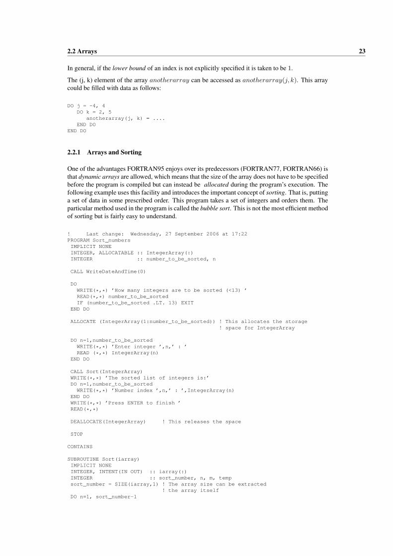
One of the advantages FORTRAN95 enjoys over its predecessors (FORTRAN77, FORTRAN66) isthat dynamic arrays are allowed, which means that the size of the array does not have to be specifiedbefore the program is compiled but can instead be allocated during the program’s execution. Thefollowing example uses this facility and introduces the important concept of sorting. That is, puttinga set of data in some prescribed order. This program takes a set of integers and orders them. Theparticular method used in the program is called the bubble sort. This is not the most efficient methodof sorting but is fairly easy to understand.
! Last change: Wednesday, 27 September 2006 at 17:22PROGRAM Sort_numbersIMPLICIT NONEINTEGER, ALLOCATABLE :: IntegerArray(:)INTEGER :: number_to_be_sorted, n
CALL WriteDateAndTime(0)
DOWRITE(*,*) ’How many integers are to be sorted (<13) ’READ(*,*) number_to_be_sortedIF (number_to_be_sorted .LT. 13) EXIT
END DO
ALLOCATE (IntegerArray(1:number_to_be_sorted)) ! This allocates the storage! space for IntegerArray
DO n=1,number_to_be_sortedWRITE(*,*) ’Enter integer ’,n,’ : ’READ (*,*) IntegerArray(n)
END DO
CALL Sort(IntegerArray)WRITE(*,*) ’The sorted list of integers is:’DO n=1,number_to_be_sorted
WRITE(*,*) ’Number index ’,n,’ : ’,IntegerArray(n)END DOWRITE(*,*) ’Press ENTER to finish ’READ(*,*)
DEALLOCATE(IntegerArray) ! This releases the space
STOP
CONTAINS
SUBROUTINE Sort(iarray)IMPLICIT NONEINTEGER, INTENT(IN OUT) :: iarray(:)INTEGER :: sort_number, n, m, tempsort_number = SIZE(iarray,1) ! The array size can be extracted
! the array itselfDO n=1, sort_number-1
2.2 Arrays 24
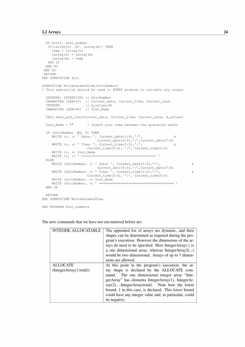
DO m=n+1, sort_numberIF(iarray(n) .GT. iarray(m)) THEN
temp = iarray(n)iarray(n) = iarray(m)iarray(m) = temp
END IFEND DOEND DORETURNEND SUBROUTINE Sort
SUBROUTINE WriteDateAndTime(UnitNumber)! This subroutine should be used in EVERY program to validate any output
INTEGER, INTENT(IN) :: UnitNumberCHARACTER (LEN=10) :: Current_date, Current_time, Current_zoneINTEGER :: d_values(8)CHARACTER (LEN=40) :: Your_Name
CALL date_and_time(Current_date, Current_time, Current_zone, d_values)
Your_Name = "" ! Insert your name between the quotation marks
IF (UnitNumber .EQ. 0) THENWRITE (*, *) ’ Date: ’, Current_date(1:4),’/’, &
Current_date(5:6),’/’,Current_date(7:8)WRITE (*, *) ’ Time: ’, Current_time(1:2),’:’, &
Current_time(3:4), ’:’, Current_time(5:6)WRITE (*, *) Your_NameWRITE (*, *) ’ ====================================== ’
ELSEWRITE (UnitNumber, *) ’ Date: ’, Current_date(1:4),’/’, &
Current_date(5:6),’/’,Current_date(7:8)WRITE (UnitNumber, *) ’ Time: ’, Current_time(1:2),’:’, &
Current_time(3:4), ’:’, Current_time(5:6)WRITE (UnitNumber, *) Your_NameWRITE (UnitNumber, *) ’ ====================================== ’
END IF
RETURNEND SUBROUTINE WriteDateAndTime
END PROGRAM Sort_numbers
The new commands that we have not encountered before are:
INTEGER, ALLOCATABLE The appended list of arrays are dynamic, and theirshapes can be determined as required during the pro-gram’s execution. However the dimensions of the ar-rays do need to be specified. Here IntegerArray(:) isa one dimensional array, whereas IntegerArray2(:,:)would be two dimensional. Arrays of up to 7 dimen-sions are allowed.
ALLOCATE(IntegerArray(1:total))
At this point in the program’s execution, the ar-ray shape is declared by the ALLOCATE com-mand. The one dimensional integer array “Inte-gerArray” has elements IntegerArray(1), IntegerAr-ray(2). . . IntegerArray(total). Note how the lowerbound, 1 in this case, is declared. This lower boundcould have any integer value and, in particular, couldbe negative.
2.2 Arrays 25
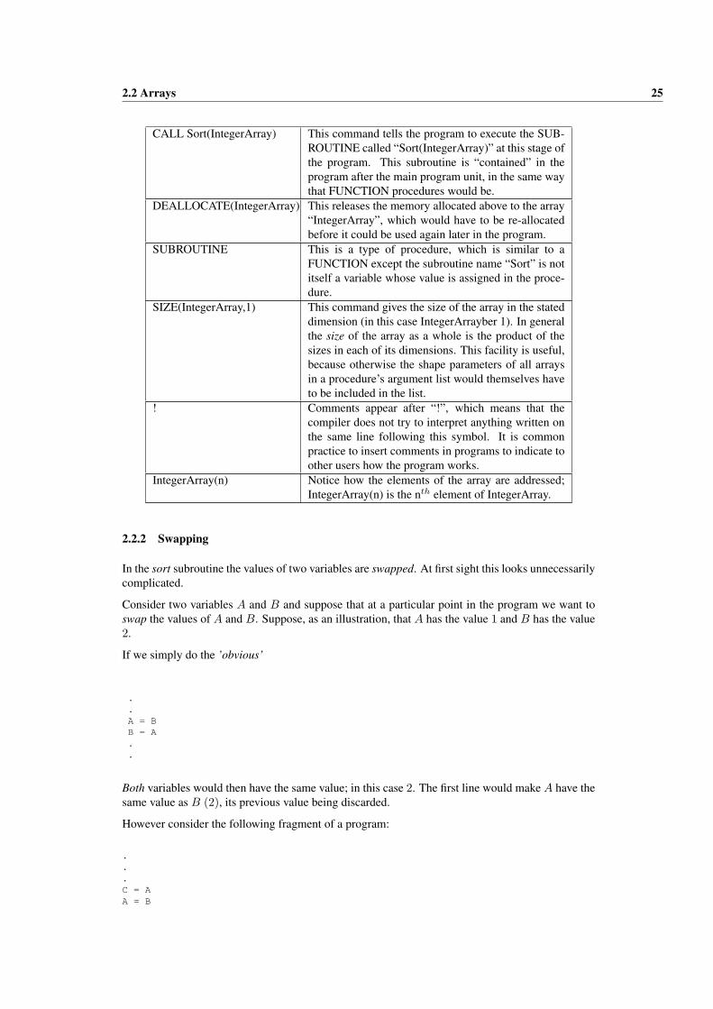
CALL Sort(IntegerArray) This command tells the program to execute the SUB-ROUTINE called “Sort(IntegerArray)” at this stage ofthe program. This subroutine is “contained” in theprogram after the main program unit, in the same waythat FUNCTION procedures would be.
DEALLOCATE(IntegerArray) This releases the memory allocated above to the array“IntegerArray”, which would have to be re-allocatedbefore it could be used again later in the program.
SUBROUTINE This is a type of procedure, which is similar to aFUNCTION except the subroutine name “Sort” is notitself a variable whose value is assigned in the proce-dure.
SIZE(IntegerArray,1) This command gives the size of the array in the stateddimension (in this case IntegerArrayber 1). In generalthe size of the array as a whole is the product of thesizes in each of its dimensions. This facility is useful,because otherwise the shape parameters of all arraysin a procedure’s argument list would themselves haveto be included in the list.
! Comments appear after “!”, which means that thecompiler does not try to interpret anything written onthe same line following this symbol. It is commonpractice to insert comments in programs to indicate toother users how the program works.
IntegerArray(n) Notice how the elements of the array are addressed;IntegerArray(n) is the nth element of IntegerArray.
2.2.2 Swapping
In the sort subroutine the values of two variables are swapped. At first sight this looks unnecessarilycomplicated.
Consider two variables A and B and suppose that at a particular point in the program we want toswap the values of A and B. Suppose, as an illustration, that A has the value 1 and B has the value2.
If we simply do the ’obvious’
.
.A = BB = A..
Both variables would then have the same value; in this case 2. The first line would make A have thesame value as B (2), its previous value being discarded.
However consider the following fragment of a program:
.
.
.C = AA = B
2.2 Arrays 26
B = C..
In this case the value of A is first put into the variable C, which is just used as temporary storage;then A takes on the value of B; and finally B takes on the original value of A which has beentemporarily stored in C.
2.2.3 Defined Types and More Sorting
Now I am now going to consider sorting more complicated objects. First I need to create a morecomplicated object. Fortran 95 has a few ’built-in’ types: INTEGER, REAL, COMPLEX, CHAR-ACTER and LOGICAL. You have not used all these yet but you will.
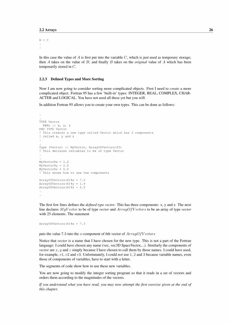
In addition Fortran 95 allows you to create your own types. This can be done as follows:
.
.TYPE Vector
REAL :: x, y, zEND TYPE Vector! This creates a new type called Vector which has 3 components! called x, y and z..Type (Vector) :: MyVector, ArrayOfVectors(25)! This declares variables to be of type Vector..MyVector%x = 1.2MyVector%y = 2.6MyVector%z = 0.0! This shows how to use the components
ArrayOfVectors(6)%x = 7.3ArrayOfVectors(6)%y = 1.9ArrayOfVectors(6)%z = 2.5..
The first few lines defines the defined type vector. This has three components: x, y and z. The nextline declares MyV ector to be of type vector and ArrayOfV ectors to be an array of type vectorwith 25 elements. The statement
ArrayOfVectors(6)%x = 7.3
puts the value 7.3 into the x-component of 6th vector of ArrayOfV ectors
Notice that vector is a name that I have chosen for the new type. This is not a part of the Fortranlanguage: I could have chosen any name (vec, vec3D SpaceVector,...). Similarly the components ofvector are x, y and z simply because I have chosen to call them by those names. I could have used,for example, v1, v2 and v3. Unfortunately, I could not use 1, 2 and 3 because variable names, eventhose of components of variables, have to start with a letter.
The segments of code show how to use these new variables.
You are now going to modify the integer sorting program so that it reads in a set of vectors andorders them according to the magnitudes of the vectors.
If you understand what you have read, you may now attempt the first exercise given at the end ofthis chapter.
2.3 Whole array expressions 27
2.3 Whole array expressions
In computational physics we very often deal with arrays. Vectors, both three-dimensional and four-dimensional space-time vectors, and matrices are examples of arrays.
FORTRAN 95 contains useful features that allow operations to be performed on all the elementsof an array in parallel. Some examples are given in the following simple program. The featureRESHAPE which is used in this program needs some explanation.
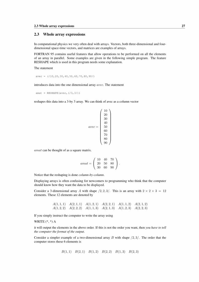
The statement
avec = (/10,20,30,40,50,60,70,80,90/)
introduces data into the one dimensional array avec. The statement
amat = RESHAPE(avec,(/3,3/))
reshapes this data into a 3-by 3 array. We can think of avec as a column vector
avec =
102030405060708090
amat can be thought of as a square matrix.
amat =
10 40 7020 50 8030 60 90
.
Notice that the reshaping is done column-by-column.
Displaying arrays is often confusing for newcomers to programming who think that the computershould know how they want the data to be displayed.
Consider a 3-dimensional array A with shape /2, 2, 3/. This is an array with 2 × 2 × 3 = 12elements. These 12 elements are denoted by
A(1, 1, 1) A(2, 1, 1) A(1, 2, 1) A(2, 2, 1) A(1, 1, 2) A(2, 1, 2)A(1, 2, 2) A(2, 2, 2) A(1, 1, 3) A(2, 1, 3) A(1, 2, 3) A(2, 2, 3)
If you simply instruct the computer to write the array using
WRITE (*, *) A
it will output the elements in the above order. If this is not the order you want, then you have to tellthe computer the format of the output.
Consider a simpler example of a two-dimensional array B with shape /2, 3/. The order that thecomputer stores these 6 elements is
B(1, 1) B(2, 1) B(1, 2) B(2, 2) B(1, 3) B(2, 3)
2.3 Whole array expressions 28
and the instruction
WRITE (*, *) B
will result in the the six elements being written to the screen in the above order.
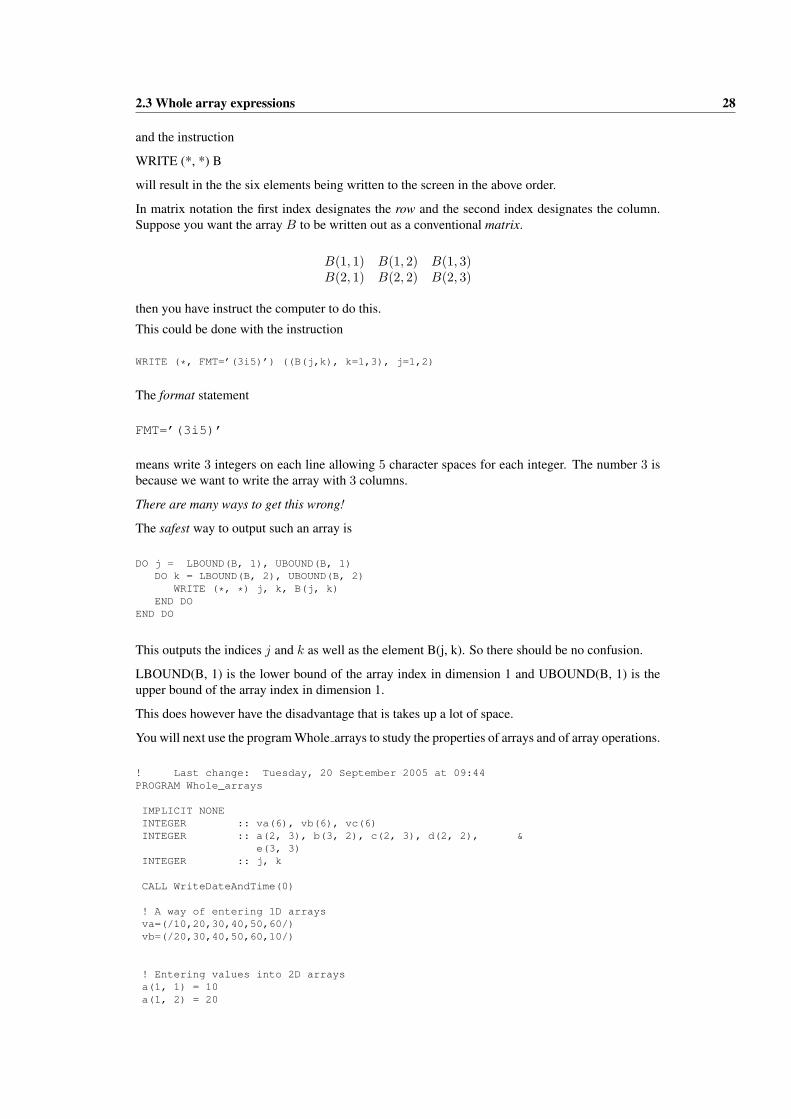
In matrix notation the first index designates the row and the second index designates the column.Suppose you want the array B to be written out as a conventional matrix.
B(1, 1) B(1, 2) B(1, 3)B(2, 1) B(2, 2) B(2, 3)
then you have instruct the computer to do this.
This could be done with the instruction
WRITE (*, FMT=’(3i5)’) ((B(j,k), k=1,3), j=1,2)
The format statement
FMT=’(3i5)’
means write 3 integers on each line allowing 5 character spaces for each integer. The number 3 isbecause we want to write the array with 3 columns.
There are many ways to get this wrong!
The safest way to output such an array is
DO j = LBOUND(B, 1), UBOUND(B, 1)DO k = LBOUND(B, 2), UBOUND(B, 2)
WRITE (*, *) j, k, B(j, k)END DO
END DO
This outputs the indices j and k as well as the element B(j, k). So there should be no confusion.
LBOUND(B, 1) is the lower bound of the array index in dimension 1 and UBOUND(B, 1) is theupper bound of the array index in dimension 1.
This does however have the disadvantage that is takes up a lot of space.
You will next use the program Whole arrays to study the properties of arrays and of array operations.
! Last change: Tuesday, 20 September 2005 at 09:44PROGRAM Whole_arrays
IMPLICIT NONEINTEGER :: va(6), vb(6), vc(6)INTEGER :: a(2, 3), b(3, 2), c(2, 3), d(2, 2), &
e(3, 3)INTEGER :: j, k
CALL WriteDateAndTime(0)
! A way of entering 1D arraysva=(/10,20,30,40,50,60/)vb=(/20,30,40,50,60,10/)
! Entering values into 2D arraysa(1, 1) = 10a(1, 2) = 20
2.3 Whole array expressions 29
a(1, 3) = 30a(2, 1) = 40a(2, 2) = 50a(2, 3) = 60 ! a has 2 rows & 3 columns
b(1, 1) = 60b(1, 2) = 50b(2, 1) = 40b(2, 2) = 30b(3, 1) = 20b(3, 2) = 10 ! b has 3 rows & 2 columns
! Using RESHAPE to enter data into a 1D array and then reshaping! this into the desired arrayvc=(/30,40,50,60,10,20/)c = RESHAPE(vc, (/2, 3/))
! You write out a 2D array in detail as followsWRITE(*, *) ’ Matrix a in detail ’DO j = LBOUND(a, 1), UBOUND(a, 1)
DO k = LBOUND(a, 2), UBOUND(a, 2)WRITE (*, *) j, k, a(j, k)
END DOEND DO
! To just write out the elements of the arrayWRITE(*, *) ’ Matrix a elements ’WRITE(*, *) a
! To write out elements in the usual matrix orderWRITE(*, *) ’ Matrix a elements in rows & columns’WRITE(*, ’(3i5)’) ((a(j,k), k=1,3), j=1,2)
! In this line each 3 represents the number of columns and! each 2 represents the number of rows
WRITE (*, *) ’ ’WRITE (*, *) ’ Press return to continue’READ (*, *)
WRITE(*, *) ’ ’WRITE(*, *) ’ Matrix b = ’WRITE(*, ’(2i5)’) ((b(j,k), k=1,2), j=1,3)
WRITE(*, *) ’ ’WRITE(*, *) ’ Matrix c = ’WRITE(*, ’(3i5)’) ((c(j,k), k=1,3), j=1,2)
! Now investigation matrix addition! Notice that a & c have the same shape so it makes sense to add themWRITE(*, *) ’ ’WRITE(*, *) ’ The sum a + c = ’c = a + c ! This adds a & c and put the sum into c
WRITE(*, ’(3i5)’) ((c(j,k), k=1,3), j=1,2)
! Now investigate element-by-element multiplication (remember that! c has changed)WRITE(*, *) ’ ’WRITE(*, *) ’ The element-by-element product a*c = ’c = a*c ! This muliplies each element of a by the
! corresponding element of c and puts the! result into c
WRITE(*, ’(3i5)’) ((c(j,k), k=1,3), j=1,2)
! Note that this is not the same as matrix multiplication
! Matrix multiplication can be done using the built-in function MATMUL
2.4 Computational Techniques 30
d = MATMUL(a, b)e = MATMUL(b, a)
! Insert code to output these product matrices
WRITE (*, *) ’ Press RETURN to continue ’READ(*,*)
STOP
CONTAINS
SUBROUTINE WriteDateAndTime(UnitNumber)INTEGER, INTENT(IN) :: UnitNumberCHARACTER (LEN=10) :: Current_date, Current_time, Current_zoneINTEGER :: d_values(8)CALL date_and_time(Current_date, Current_time, Current_zone, d_values)
IF (UnitNumber .EQ. 0) THENWRITE (*, *) ’ Date: ’, Current_date(1:4),’/’, &
Current_date(5:6),’/’,Current_date(7:8)WRITE (*, *) ’ Time: ’, Current_time(1:2),’:’, &
Current_time(3:4), ’:’, Current_time(5:6)WRITE (*, *) ’ ====================================== ’
ELSEWRITE (UnitNumber, *) ’ Date: ’, Current_date(1:4),’/’, &
Current_date(5:6),’/’,Current_date(7:8)WRITE (UnitNumber, *) ’ Time: ’, Current_time(1:2),’:’, &
Current_time(3:4), ’:’, Current_time(5:6)WRITE (UnitNumber, *) ’ ====================================== ’
END IF
RETURNEND SUBROUTINE WriteDateAndTime
END PROGRAM Whole_arrays
If you understand what you have read, you may now attempt the second exercise given at the end ofthis chapter.
2.4 Computational Techniques
I have already introduced at one useful technique: sorting. Now I introduce a few more.
2.4.1 Summations
Suppose I need to find the sum of a (possibly large) number of quantities. First I need a variable tohold the summation: I call this Total. Then I add the contributions to Total one by one. This couldbe done as follows:
.
.INTEGER :: j, nREAL :: Total..Total = 0.0DO j = 1, n
Total = Total + ...END DO..
2.4 Computational Techniques 31
where . . . contains the formula for calculating the j th element of the summation.
If the quantities to be summed have been put into an array then Fortran 95 has a built-in mechanismfor summation:
.
.INTEGER :: n, n1, n2, n3REAL :: Total1, Total2, Total3..Total1 = SUM(S(1:n))Total2 = SUM(T(n1:n2))Total3 = SUM(U(n1:n2, n3)).
In this case Total1 is the sum of the elements 1, . . . , n of one dimensional array S; Total2 is thesum of the elements n1, . . . , n2 of one dimensional array T; and Total3 is the sum of the elementsn1, . . . , n2 of the n3th column of two dimensional array U.
Note that the arrays S, T , U also have to be declared. These can be declared with fixed sizes ordeclared as ALLOCATABLE (and then ALLOCATED).
2.4.2 Integration
Suppose now that I need to evaluate the integral∫ b
a
dx f (x)
In general I can approximate an integral by means of the trapezoidal rule. The essence of this is asfollows:
The range of the integral is divided into N equal intervals of size δx (= (b−a)/N) and the functionis evaluated at co-ordinates
xj = a + jδx j = 0, . . . , N
Between these co-ordinates the function (integrand) is approximated by a sequence of straight-linesegments.
The result for the integral is
(b− a)N
12
(f (x0) + f (xN )) +N−1∑j=1
f (xj)
Clearly the summation techniques introduced above can be used to carry this out.
In principle, the smaller δx the better the approximation. However, because of the finite numericalprecision, decreasing δx below some value will start to make the approximation worse.
2.4.3 Differentiation
Differentiation is used throughout physics. In order to evaluate a derivative numerically, I make useof the formal definition:
df (x)dx
= limδx→0
f
(x +
δx
2
)− f
(x− δx
2
)δx
2.5 Graphics 32
The approximation to this suitable for computation is obtained by taking δx to be small but not zero.Generally the approximation gets better as δx gets smaller but you should always be aware of thelimitations of computers. (Remember the program numerical.f95!)
The corresponding expression for the second derivative can also be obtained from the above formula
by replacing f bydf
dxon the right-hand side:
d2f (x)dx2
= limδx→0
df
dx
(x +
δx
2
)− df
dx
(x− δx
2
)δx
= limδx→0f (x + δx) + f (x− δx)− 2f (x)
δx2
In practice it is much better to use a higher precision than the standard Real kind.
Now attempt exercise 3.
2.5 Graphics
There are no standard graphics facilities available in FORTRAN 95. Instead each compiler maycome with its own graphics routines. The following subroutine, which is used in the programStline.f95, makes use of the Salford software’s graphics. The subroutine plots the data pointsx(n), y(n) as circles and draw the least-squares-fit line for the points which has gradient s and in-tercept c. With the comments the graphics commands may be self-explanatory! The main elementof the graphics is the drawing subroutine:
CALL draw_line@(x1, y1, x2, y2, RGB@(200, 0, 0))
This draws a line from (x1, y1) to (x2, y2) in a colour specified by its Red, Green & Blue intensities.(0, 0, 0)=black, (255, 255, 255)=white, (255, 0, 0)=red, etc.
The co-ordinates are integer variables and are in pixels. (0, 0) is the top left of the window.
Don’t worry too much about the details of this graphics subroutine but make sure you can identifythe actual drawing instructions.
SUBROUTINE plotgraph(x, y, s, c, deltas, rotated)
USE MSWINIMPLICIT NONEREAL (KIND=P), INTENT(IN) :: x(:), y(:), s, c, deltasLOGICAL, INTENT(IN) :: rotatedINTEGER :: n, j, intg, handle1, ctrl1REAL (KIND=P), ALLOCATABLE :: cx(:), cy(:)REAL (KIND=P) :: xmin, xmax, ymin, ymax, xavg, yavgREAL (KIND=P) :: ystart, yendREAL (KIND=P) :: gscaleREAL (KIND=P) :: ninetydegrees=90.0PINTEGER (KIND=3) :: fullscreenheight,fullscreenwidth, &
graphics_width, graphics_heightINTEGER (KIND=3) :: graphics_top, graphics_bottom, &
graphics_left, graphics_right, &graphics_x, graphics_y
CHARACTER (LEN=20) :: string
n = SIZE(x, 1) ! n is the size of the array x
2.5 Graphics 33
! Allocate space for arrays cx, cy which are copies of x & yALLOCATE (cx(1:n), cy(1:n))
IF (rotated) THENcx = REAL(y, KIND(1.0))cy = REAL(x, KIND(1.0))
ELSEcx = REAL(x, KIND(1.0))cy = REAL(y, KIND(1.0))
END IF
! Find the minimum and maximum values of cx & cyxmin = MINVAL(cx(:))xmax = MAXVAL(cx(:))ymin = MINVAL(cy(:))ymax = MAXVAL(cy(:))
! Open Window with 2 panels
intg = winio@(’%ca[Computational Physics---StLine]&’)intg = winio@(’%1.2ob[panelled]&’) ! 1.2 means 1-by-2
! Find screen resolutionfullscreenwidth = Clearwininfo@(’ScreenWidth’)fullscreenheight = Clearwininfo@(’ScreenDepth’)
WRITE (*, *) fullscreenwidth,fullscreenheight
! Choose a window size which a fraction of full screen
gscale = 0.6
graphics_height = INT(fullscreenheight*gscale)
graphics_width = INT(fullscreenwidth*gscale)
! Put graphics window in top panel
! Set handle for window --- only really necessary if more than one! graphics window is usedhandle1 = 999 ! Arbitrary integer but different from other
! window ‘handles’
intg = winio@(’%‘gr[white, rgbcolours] %cb&’,graphicswidth, &graphics_height, handle1)
intg = winio@(’%ww%lw&’, ctrl1)
! Put title in bottom panelintg = winio@(’%18bt[Straight Line Fit] %cb’)
! Set limits of plotting framegraphics_top = INT(0.1*graphics_height)graphics_bottom = INT(0.8*graphics_height)graphics_left = INT(0.2*graphics_width)graphics_right = INT(0.9*graphics_width)
! Plot points
intg = select_graphics_object@(handle1)
! Start copying graphics to metafileintg = open_metafile@(handle1)
DO j = 1, ngraphics_x = INT((cx(j)*(graphics_right-graphics_left) + &
(graphics_left*xmax-graphics_right*xmin))/ &(xmax-xmin))
graphics_y = INT((cy(j)*(graphicstop-graphics_bottom) + &(graphics_bottom*ymax-graphicstop*ymin))/ &
2.6 Exercises 34
(ymax-ymin))CALL fill_ellipse@(graphics_x, graphics_y, 2, 2, RGB@(100,0, 200))
END DO
! Draw axesCALL draw_line@(graphics_left, graphics_bottom,graphics_right, &
graphics_bottom, RGB@(0,0,0))CALL draw_line@(graphics_left, graphics_bottom,graphics_left, &
graphics_top, RGB@(0,0,0))CALL draw_line@(graphics_left, graphics_top,graphics_right, &
graphics_top, RGB@(0,0,0))CALL draw_line@(graphics_right, graphics_bottom,graphics_right, &
graphics_top, RGB@(0,0,0))
! Draw straight-line fitystart = s*xmin + cyend = s*xmax + cCALL draw_line@(graphics_left, &
INT((ystart*(graphicstop-graphics_bottom) + &(graphics_bottom*ymax-graphicstop*ymin))/ &(ymax-ymin)), graphics_right, &INT((yend*(graphic_stop-graphics_bottom) + &(graphics_bottom*ymax-graphicstop*ymin))/ &(ymax-ymin)), RGB@(0,0,0))
! Draw straight-lines with uncertainties here
! Write labels for axes
string = ‘ x-axis’CALL rotatefont@(0.02)CALL drawtext@(string, graphics_left+30,graphics_bottom+20,RGB@(0,0,0))
string = ‘ y-axis’CALL rotatefont@(ninetydegrees)CALL drawtext@(string, graphics_left,graphics_bottom,RGB@(0,0,0))
! Copy metafile to clipboard -- you can then use Word to! capture and print this
! Stop recording the graphicsintg = metafile_to_clipboard@()intg = close_metafile@(handle1)
DEALLOCATE (cx, cy)
RETURN
END SUBROUTINE plot_graph
If you think you understand the drawing features of this subroutine, proceed to exercise 4.
2.6 Exercises
1. [4 Marks](a) Compile and execute the Sort numbers.f95 program. Check that it works
properly by entering a few sets of integers. In order to understand how theprogramme works take a set of four integers (11 5 9 7) and perform (andrecord) each of the operations of the sort subroutine manually. There are 6such operations in this case.Remember to keep a record of your work in your logbooks.

2.6 Exercises 35
(b) Make a copy of the program, and modify it as follows: Change the relevantvariables from INTEGER to TYPE (vector). The criterion for sorting involvesthe magnitudes of the vectors: The magnitude of vector A is SQRT (A%x ∗∗2+A%y∗∗2+A%z∗∗2). Allow the user to enter a set (totalnumber < 12)of vectors, and then order these in terms of their magnitudes. Note: Youshould end up with an ordered list of the vectors not just their magnitudes.Record your tests.
2. [4 Marks](a) Compile and execute the Whole arrays.f95 program and verify that the
element-by-element addition and multiplication have worked correctly.(b) Display the results of the MATMUL operations in the program. Do the ma-
trix multiplications ’by hand’ and check that MATMUL functions work cor-rectly.
(c) Find out how the following commands work, implement them in your pro-gram and verify that they produce the correct results:DOT PRODUCT, MAXLOC, MAXVAL, TRANSPOSENotice that if if you assign MAXLOC to a variable such asm = MAXLOC(A)then the variable m must be declaredINTEGER :: m(dimA)where dimA is the number of dimensions (rank) of the array aIntroduce some new arrays into the program with negative as well as positiveindices and check that LBOUND and UBOUND work as expected.
3. [6 Marks](a) Use the two methods in the Summations section to to calculate the sum of 1
n2
from n = 5 to n = 1000 and the sum of 1n4 from n = 1 to n = 100
(b) Use the trapezoidal technique to integrate sin(x) from x = 1 to x = 10 andln(x) from x = 2 to x = 5. Use several different values for N , the numberof intervals.Record your results.
(c) Use the formulas in the Differention section to calculate the first and secondderivatives of sin(x) at x = 1 and ln(x) at x = 2. Explore a range of valuesfor δx and compare the computed results with the exact answers. Commenton your results.
4. [3 Marks](a) Compile and execute the Stline.f95 program which uses the graphics subrou-
tine Plot graph. The program ask the user to enter a set of points to which itfits the least-square line. Choose a set of data which lies approximately, butnot exactly, on a straight line. Check that the program is working correctly.
(b) The program declares the precision of its variables through the KIND state-ment. Find out about the possible precision for the variable types in theSALFORD FTN95 Help facility and record what you learn.
(c) Obtain a copy of the graph produced by the program as follows:(1) This program writes a copy of the graph to the clipboard. Open up aWORD file and paste the graph into it. The graph can now be stretched asappropriate and printed from WORD in the usual way.

2.6 Exercises 36
(d) Modify the program so that the Plot graph routine also draws lines show-ing the uncertainties in the gradient delta s. The lines should pass throughthe centre-of-mass co-ordinates of the data set (xavg, yavg). Note thatthe equation of a line with slope s which passes through (xavg, yavg) isy = yavg + s(x− xavg)
Remember that you must finish your work on this chapter by writing a summary in your logbook.This should summarize in less than 300 words what you have learnt and whether the objectives ofthis chapter have been met.
Chapter 3
EQUATIONS OF MOTION IN PHYSICS
Version date: Thursday, 30 August, 2007 at 10:06
3.1 Objectives
On completion of this chapter you will have encountered and applied some common numericalmethods for solving equations of motion which will be used later in the module. You will alsohave reviewed the behaviour of the simple harmonic oscillator and studied a particular anharmonicoscillator.
3.2 The Numerical Methods
In dynamics the equations of motion that arise in Physics are typically in the form
md2x (t)
dt2= F (3.1)
where x is a particle co-ordinate which varies with time t; and F is the force acting on the particleof mass m. In general this force will be a function of x, t and the particle’s velocity v. In this casethe problem is to find x as a function of time given the position x0 and velocity v0 at some initialtime t0. In general, this is called an initial value problem.
However before I tackle this second-order equation I first investigate the solution of a simpler, first-order equation:
dq
dt= D (3.2)
where q represents some physical quantity which varies with t and D depends on q and t. The aimhere is to find a numerical method which determines q at some time t given its value q0 at sometime t0.
I choose to try to evaluate q at a discrete set of equally spaced times
tn = t0 + nτ,
where n is an integer and τ is the time-step. As an aid to developing a numerical approximation, Ifirst write down an exact relation between neighbouring time steps:
q (tn+1) = q (tn) +∫ tn+1
tn
D (q, t) dt (3.3)
37
3.2 The Numerical Methods 38
This is obtained by integrating equation (3.2) between tn and tn+1. However there is a problem; ifI have evaluated q(t) one step at a time up to the nth step I do not know q(t) throughout the rangeof the integral in equation (3.3) but only at the initial point tn.
A crude approximation, called Euler’s method, involves simply replacing D(q(t), t) in the integralby the constant value D(q(tn), tn). This gives rise to the approximate result
q (tn+1) = q (tn) + D (q (tn) , tn) τ (3.4)
and this relation can be used to step forward in time, starting from the known value q(t0) . Howeverthis is not a very good procedure: Over long times the errors tend to accumulate rapidly.
In order to improve on this I need a better way of estimating the integral in equation (3.3). Onemethod of achieving this improvement is known as the predictor-corrector method. This hasmany variations but the simplest is as follows.
• I use the Euler method (3.4) to provide a rough estimate of q(tn+1) (this is called the predictionstage) and I denote its value by q(p)(tn+1)
• Then use this estimate to approximate the mean value of the integrand in equation (3.3) overthe range [tn, tn+1] (this is called the correction stage).
This gives a new, improved estimate of q(tn+1) :
q (tn+1) = q(p) (tn+1) +12
[D (q (tn+1) , tn+1)−D (q (tn) , tn)] τ (3.5)
The second term on the right-hand side of equation (3.5) is called the correction. In this termq(tn+1) is (initially) replaced by the prediction q(p)(tn+1). Note that the correction stage can beiterated a few times using the increasingly better estimates in the right-hand side to improve theaccuracy of the procedure. In other words q(tn+1) in the equation keeps getting replaced by thelatest estimate.
As a rough guide to the accuracy of these numerical approximations, the error in each step usingequation (3.4), the Euler approximation, is
≈ τ2
2dD
dt
whereas using equation (3.5)), the predictor-corrector method, the error in each step is
≈ τ3
12d2D
dt2
These are the errors per time step. For a fixed total time the number of time steps is inverselyproportional to τ and so in the two cases we expect the total error to be proportional to τ for theEuler method and proportianal to τ2 for the predictor-corrector method.
For a small enough step-size τ the predictor-corrector method is usually greatly superior to the Eulermethod.
I now return to the second-order equations that more often arise in Physics. Equation (3.1) can bewritten as a pair of first-order equations:
dx
dt= v
dv
dt=
F
m
(3.6)
3.3 The anharmonic oscillator 39
If I package the left-hand sides x and v as an array q (q(1) = x and q(2) = v) and package theright-hand sides v and F/m as another array D (D(1) = v and D(2) = F/m) then equations (3.6)can be written as the single equation (3.2) providing I interpret q and D as arrays of size two:
dqdt
= D ⇒ d
dt
[xv
]=[
vF/m
](3.7)
The above two approximation procedures, Euler and Predictor-Corrector, can then be applied di-rectly to this case.
This method can be extended to higher-order differential equations, so that (3.2) can in fact be usedto solve an N th order (initial value) differential equation.
The Euler and Predictor-Corrector methods are supplied as subroutines in the program ‘diffequ.f95’.This program can be used to test the procedures: It is set up to solve the harmonic oscillator equa-tion:
d2x
dt2= −ω0
2x
This is useful for testing purposes because its exact solution is known:
x (t) = x0 cos (ω0 t) +v0
ω0sin (ω0 t)
v (t) = v0 cos (ω0 t)− x0 ω0 sin (ω0 t)
where x0 and v0 are the position and velocity at time 0.
In the program the angular frequency ω0 is set to one. So the period of the motion should be 2π.
If you think you understand what you have read, you may now attempt exercise 1 at the end of thischapter.
3.3 The anharmonic oscillator
Consider now the example of an anharmonic oscillator. The equation of motion for this system is
d2x
dt2= −x3 (3.8)
where as usual x is the displacement of the oscillator from its equilibrium position at time t.
You are going to investigate the motion of this oscillator starting it from a position x0 with zerovelocity.
In this case it is not possible (as far as I know!) to write the exact solution and we are going to usethe programs to determine the solutions. We are now using the program to help us with physicswhereas with the harmonic oscillator we were using a known physics result to test the program.
In the harmonic oscillator the motion is periodic with a period (2π in the above case) which isindependent of the starting position.
However, in the anharmonic oscillator you should find that the motion is periodic but with with aperiod which does depend on x0. You are going to investigate the dependence of the period on x0.
3.4 Exercises 40
3.3.1 Determination of the period
The period can be determined by finding when the particle first returns to its initial position x0.However you will determine the position at discrete time intervals and so the chance of hitting x0
exactly is remote.
A more precise method is as follows:
(i) First identify approximately the period and the nearest space-time point – call this (x2, t2)(ii) Call the two neighbouring space-time points (x1, t1) and (x3, t3) where t1 < t2 < t3.(iii) Identify the period using the formula:
T =
((x3 − x2)
(t22 − t21
)− (x2 − x1)
(t23 − t22
))2 ((x3 − x2) (t2 − t1)− (x2 − x1) (t3 − t2))
The formula was obtained by fitting a parabola to these three space-time points. Note that theresulting period should lie in the range (t1, t3). If it does not then you have made some error inimplementing the formula.
If you think you understand what you have read, you may now attempt exercises 2 and 3 below.
3.4 Exercises
1. [10 Marks](a) [2 marks] Compile and run the program ‘diffequ.f95’. It is set up
to find the solution, that is position and velocity as a function oftime, for the simple harmonic oscillator. The characteristic angularfrequency ω0 is set to 1 in this program. Enter a final time (as a num-ber of periods, say 6); and a reasonably small step-size, say 0.025.Choose the Euler method. Browse the program to get a rough ideaof how it works. Investigate, and record, the effect on the relativerms errors of halving and doubling your initial time step.
(b) [2 marks] You are now going to explore the Euler method inmore detail. Choose a set of, about 12, step-sizes in the range1.0 × 10−6 · · · 1.0 × 10⁻¹ and tabulate the relative rms errors foreach.Note: For the smaller step sizes you might want to reduce the amountof output. This can be done by changing the line ”IF (4*(istep/4).EQ. istep) THEN” to ”IF (NP*(istep/NP) .EQ. istep) THEN” whereNP is some integer much larger than 4.
(c) [1 mark] Using Excel, or otherwise, plot the errors against the time-step on a log-log plot. If the rms error is roughly proportional tosome power say, (stepsize)ne , then the slope of the log-log plot willbe equal to ne.
3.4 Exercises 41
(d) [4 marks] Now repeat the exercises (b) and (c) but using thePredictor-Corrector procedure. First with one iteration of the cor-rection stage then two.In most practical applications of these methods it is the determina-tion of D which is the most time-consuming part of each proce-dure. In the Euler method D is evaluated once per time-step; in thepredictor-corrector with one iteration it is evaluated twice per time-step ; and in the predictor-corrector with two iterations it is evaluatedthree time per time-step.Comparing the numerical methods you should compare the accuracywhich results from the same (or nearly the same) numerical effort. Inorder to make sensible comparisons, plot the error against a variabledtD where dtD = dt in the Euler case; dtD = 2dt in the Predictor-Corrector case with one iteration; and dtD = 3dt in the Predictor-Corrector case with two iterations. You can achieve this by using thesame set of time-steps used in (b), first multiplied by 2 and then by3.
(e) [1 mark] Comment on the results of your work and identify which isthe ’best’ method. Explain carefully how you came to this conclu-sion.
Remember to keep an accurate record of your work in your log-book.
2. [7 Marks](a) [1 marks] Download the program ’anharmonic.f95’. Read the pro-
gram and attempt to understand how it works. Run the program,using x0 = 1 and with a final time of 20.0 and a step-size of 0.025.Comment on the results.
(b) [3 marks] You are now going to investigate the dependence of theperiod of the oscillation on the starting position x0. Modify the pro-gram so at the end of each time step it writes the time and positionto a file. Choose a set of, say 10, values of x0 in the range 1 − 10.For each value: First check, from the graphical output, that the calcu-lated motion is periodic. If the amplitude grows or decays it probablymeans that your step size is too large. Experiment with different step-sizes and record your observations. Experiment with the final timeuntil the graphical display shows just over one period. Then use theformula given in the text to obtain an accurate value for the period.Tabulate the x0-period pairs (together with the time-steps you used).
(c) [3 marks] Using Excel, or otherwise, produce a graph of periodagainst starting position. Explore ways of plotting the data in or-der to identify the precise dependence of the period on x0. That is,get a formula for the period as a function of x0.
Remember that you must finish your work on this chapter by writing a summary in yourlogbook. This should summarize in less than 300 words what you have learnt and whether theobjectives of this chapter have been met.
Chapter 4
PLANETARY MOTION
Version date: Thursday, 28 September 2006 at 13:36
4.1 Objectives
In this section you will investigate the motion of planets in the solar system.
On completion of this chapter you will have gained experience in applying numerical methods forsolving equations of motion of planets and have explored the nature of the orbits; and you shouldunderstand the significance of the conservation of angular momentum. You should also know howconservation laws can be used to explore the accuracy of the numerical procedures.
You should also have gained experience in using the editor (to re-use code from other programmes);and in manipulating data in files.
4.2 Equations of Motion.
I shall take a simplified view of the solar system in which I assume the mass of the Sun is so muchlarger than that of any planet that I can neglect the effects of the planets on each other and canneglect the motion of the Sun.
The mass of the largest planet is about one thousandth of the mass of the Sun and so, in general, thisapproximation should be accurate to about one part in one thousand. However in “our neighbour-hood” the planets are smaller and the approximation is better than this.
In this approximation the force on a given planet is only due to the Sun and so Newton’s equationfor the motion of the planet is
md2rdt2
= −GmMSrr3
(4.1)
where r is the position vector of the planet, r is its magnitude, G is the gravitational constant andMS is the mass of the Sun which is at the origin of the co-ordinate system.
4.3 Conservation of Angular Momentum
I first show that the angular momentum of the planet is conserved and look at the consequences ofthis.
It is useful to define the vector h,
h = r ∧ drdt
(4.2)
42
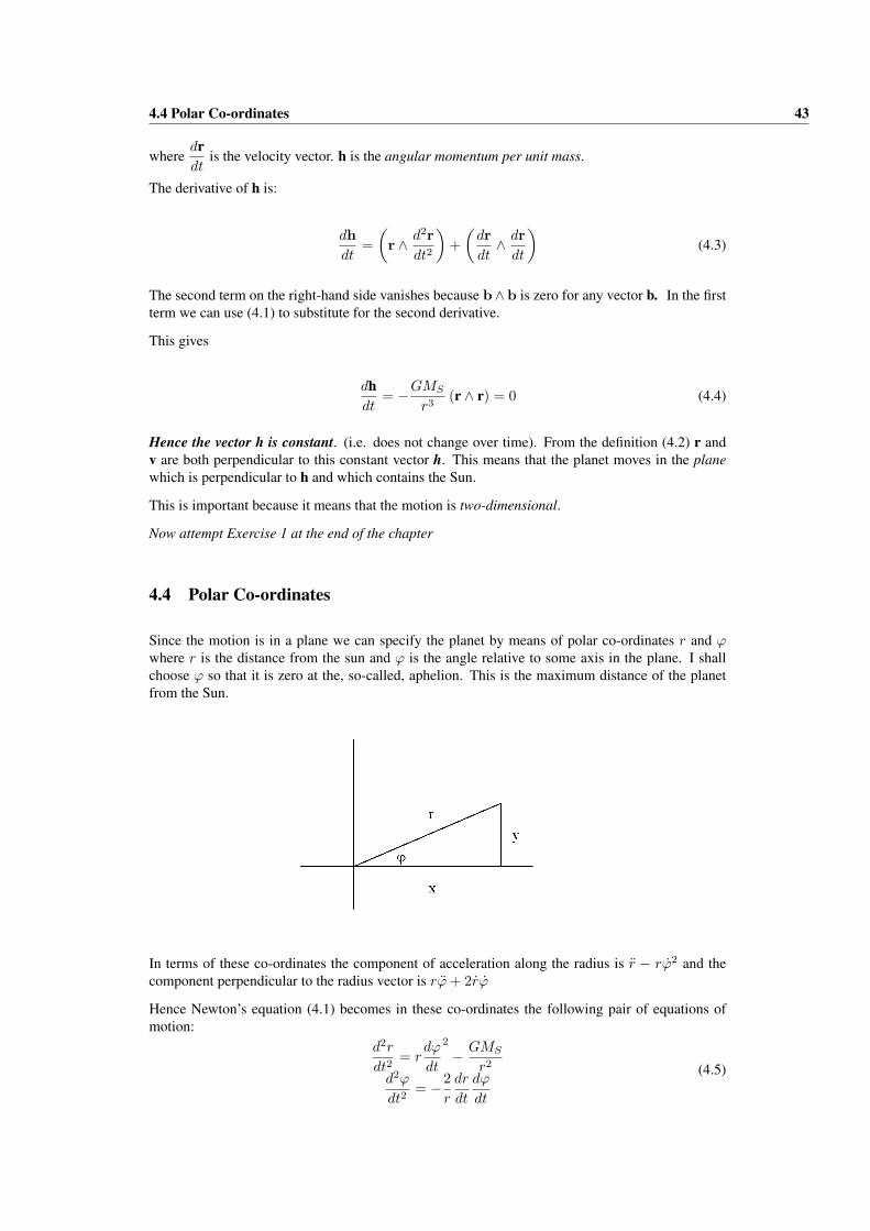
4.4 Polar Co-ordinates 43
wheredrdt
is the velocity vector. h is the angular momentum per unit mass.
The derivative of h is:
dhdt
=(r ∧ d2r
dt2
)+(
drdt∧ dr
dt
)(4.3)
The second term on the right-hand side vanishes because b∧b is zero for any vector b. In the firstterm we can use (4.1) to substitute for the second derivative.
This gives
dhdt
= −GMS
r3(r ∧ r) = 0 (4.4)
Hence the vector h is constant. (i.e. does not change over time). From the definition (4.2) r andv are both perpendicular to this constant vector h. This means that the planet moves in the planewhich is perpendicular to h and which contains the Sun.
This is important because it means that the motion is two-dimensional.
Now attempt Exercise 1 at the end of the chapter
4.4 Polar Co-ordinates
Since the motion is in a plane we can specify the planet by means of polar co-ordinates r and ϕwhere r is the distance from the sun and ϕ is the angle relative to some axis in the plane. I shallchoose ϕ so that it is zero at the, so-called, aphelion. This is the maximum distance of the planetfrom the Sun.
In terms of these co-ordinates the component of acceleration along the radius is r − rϕ2 and thecomponent perpendicular to the radius vector is rϕ + 2rϕ
Hence Newton’s equation (4.1) becomes in these co-ordinates the following pair of equations ofmotion:
d2r
dt2= r
dϕ
dt
2
− GMS
r2
d2ϕ
dt2= −2
r
dr
dt
dϕ
dt
(4.5)
4.5 Numerical solution of equations of motion 44
4.5 Numerical solution of equations of motion
We will next set about solving these equations of motion. That is, we suppose that the co-ordinates(r,ϕ) and the velocities (r, ϕ)are known at some initial time and we want to determine the co-ordinates at succeeding times.
We are going to use the methods introduced in chapter 3. Each of the second-order equations (4.5)can be converted into two first-order equations. In order to achieve this we introduce two newvariables v – the radial velocity – and ω – the angular velocity. The four first-order equations arethen
dr
dt= v
dv
dt= rω2 − GMS
r2
dϕ
dt= ω
dω
dt= −2
r
dr
dt
dϕ
dt
(4.6)
We can express these equations in the condensed form
dq
dt= D (4.7)
where q and D are column vectors with elements:
q =
rvϕω
(4.8)
D =
v
rω2 − GMS
r2
ω
−2rvω
(4.9)
4.6 Energy and Angular Momentum
With a little more effort we could have done some integration on equations (4.5) to obtain the twoconserved quantities:
h = r2ω
E =12(v2 + r2ω2
)− GMS
r
(4.10)
The first of these is the angular momentum (per unit mass) introduced above and the second is theenergy per unit mass.
If we could solve the equations with absolute precision, the right hand sides of (4.10) would beindependent of time. In practice this will not be so. However the relative variation in these righthand sides gives us useful information about the accuracy of the whole numerical procedure.
If we evaluate the right-hand sides of these expressions for h and E at each step in the numericalprocedure then we have a measure of the accuracy of the procedure. The maximum value of therelative error in h or E can be used as an estimate of the accuracy of the overall calculation.
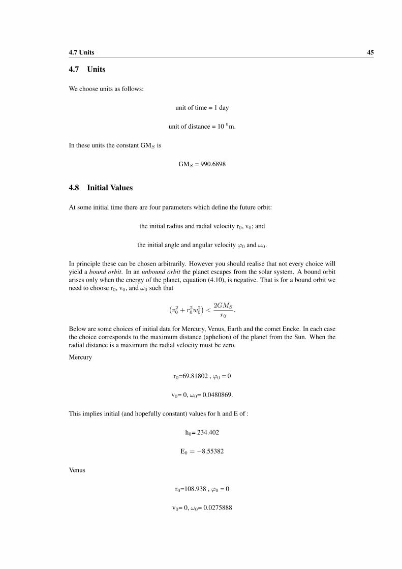
4.7 Units 45
4.7 Units
We choose units as follows:
unit of time = 1 day
unit of distance = 10 9m.
In these units the constant GMS is
GMS = 990.6898
4.8 Initial Values
At some initial time there are four parameters which define the future orbit:
the initial radius and radial velocity r0, v0; and
the initial angle and angular velocity ϕ0 and ω0.
In principle these can be chosen arbitrarily. However you should realise that not every choice willyield a bound orbit. In an unbound orbit the planet escapes from the solar system. A bound orbitarises only when the energy of the planet, equation (4.10), is negative. That is for a bound orbit weneed to choose r0, v0, and ω0 such that
(v20 + r2
0w20
)<
2GMS
r0.
Below are some choices of initial data for Mercury, Venus, Earth and the comet Encke. In each casethe choice corresponds to the maximum distance (aphelion) of the planet from the Sun. When theradial distance is a maximum the radial velocity must be zero.
Mercury
r0=69.81802 , ϕ0 = 0
v0= 0, ω0= 0.0480869.
This implies initial (and hopefully constant) values for h and E of :
h0= 234.402
E0 = −8.55382
Venus
r0=108.938 , ϕ0 = 0
v0= 0, ω0= 0.0275888
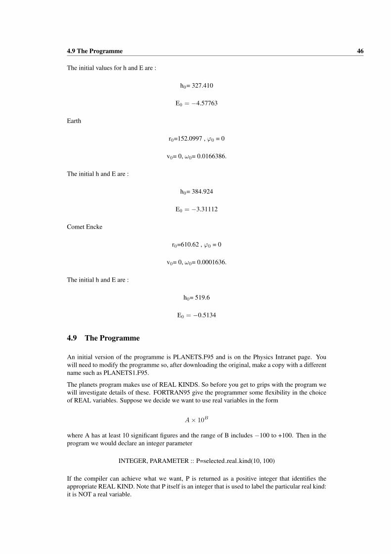
4.9 The Programme 46
The initial values for h and E are :
h0= 327.410
E0 = −4.57763
Earth
r0=152.0997 , ϕ0 = 0
v0= 0, ω0= 0.0166386.
The initial h and E are :
h0= 384.924
E0 = −3.31112
Comet Encke
r0=610.62 , ϕ0 = 0
v0= 0, ω0= 0.0001636.
The initial h and E are :
h0= 519.6
E0 = −0.5134
4.9 The Programme
An initial version of the programme is PLANETS.F95 and is on the Physics Intranet page. Youwill need to modify the programme so, after downloading the original, make a copy with a differentname such as PLANETS1.F95.
The planets program makes use of REAL KINDS. So before you get to grips with the program wewill investigate details of these. FORTRAN95 give the programmer some flexibility in the choiceof REAL variables. Suppose we decide we want to use real variables in the form
A× 10B
where A has at least 10 significant figures and the range of B includes −100 to +100. Then in theprogram we would declare an integer parameter
INTEGER, PARAMETER :: P=selected real kind(10, 100)
If the compiler can achieve what we want, P is returned as a positive integer that identifies theappropriate REAL KIND. Note that P itself is an integer that is used to label the particular real kind:it is NOT a real variable.

4.10 Kepler’s Laws 47
We can then use this integer parameter P to define REAL variables with the desired (or better)precision:
REAL (KIND=P) :: a, b, c
We can also use constants in the program to this precision as follows:
1.0 P, ,2.5 P
Notice that if we simply use 1.0 or 2.5 then these will only have the precision of the basic REALKIND (usually 6 digit accuracy).
If the compiler cannot achieve the desired accuracy then P is returned with a negative value and anyattempt to use it to define a REAL KIND will produce an error.
Now attempt Exercises 2 & 3 at the end of the chapter
4.10 Kepler’s Laws
Kepler (1571-1630) discovered his three laws of planetary motion by observation (of Brahe’s data)before Newton’s theory of gravitation. His first and second laws were published in 1609 and histhird in 1619.
First Law: Keplar’s first law states that the orbit of a planet is an ellipse with the Sun at onefocus.
How can we check whether our computed orbit is an ellipse ?
The equation of an ellipse, in the polar co-ordinates we are using, is
r =R
1− εcos (ϕ)(4.11)
where R and ε are constants defined by
R =h2
GMS(4.12)
ε =
√√√√(1 +2Eh2
(GMS)2
)(4.13)
ε is called the eccentricity. ε=0 corresponds to a circular orbit: the larger ε the more elongated theorbit. h and E are the angular momentum (per unit mass) and energy (per unit mass) defined earlier.
If we plot y=r versus x=R/(1 - εcos(ϕ)) then, if the orbit really is an ellipse, we should obtain astraight with slope 1 and abscissa 0.
Second Law: The radius vector sweeps through equal areas in equal times.
If in (small) time δt the angle ϕ changes to ϕ + δϕ then the area swept out by the radius vector isr2δϕ . Hence the area swept out per unit time is
r2 δ ϕ
δ t→ r2ϕ
Kepler’s second law implies that this is constant. However you should have already checked this(Exercise 3) under the guise of “conservation of angular momentum”.

4.11 Exercises 48
Third Law: The square of the period is proportional to the cube of the major axis.
Now attempt Exercise 4
4.11 Exercises
Exercise 1 [3 Marks]
How would the equation of motion of a particular planet change from (4.1) if we were to includeinteractions with other planets ?
The angular momentum of a particular planet will no longer be conserved if we include interactionswith other planets. Explain why and discuss the consequence for the orbit.
Exercise 2 [2 Marks]
Download the program kind test.f95 and explore the REAL KINDS that are available on the Salfordcompiler.
Exercise 3 [6 Marks]
Now download the planets.f95 program and compile and run the programme.
You will be prompted to choose a particular planet or comet; or to enter your own choice for theinitial values r0, ϕ0 ,v0 and ω0. Try the data given for Mercury, Venus, Earth and comet Encke andoutput the data to four separate files.
Record your observations. What is the period? What is the perihelion (minimum distance fromSun) and at what angle does it occur? Do this for a few time-steps and record your results.
Modify the program planets.f95 so that
h = r2ω
E = 12
(v2 + r2ω2
)− GMS
r
are evaluated initially and at each subsequent time-step. Output these values to a file.
Physics says that these two values should be constant. In fact because of the approximate calcula-tion they will fluctuate. The magnitude of the fluctuations is an indication of the accuracy of thenumerical procedure.
Use your results to estimate the accuracy of the numerical procedures for a few time steps for eachplanet.
Exercise 4: [6 Marks]
Check that the computed orbits are ellipses in the following way. In the program planets.f95 intro-duce allocatable arrays x, y and variables s, c, delta s, and delta c. Allocate the arrays x and ywith size n steps after the completion of the calculation of the orbit.
Then use a DO loop to read data into the variables x(j), y(j) from the disc file:
REWIND 15 ! This positions the file at its startDO j=1,n_steps
READ (15, FMT=’(5(2X,E14.6))’) t, q(1), q(2), q(3), q(4)! The above line should be essentially the same as the WRITE line! which stored the data! Notice that we have to read all the data in the record, even the! items we do not wanty(j) = q(1)
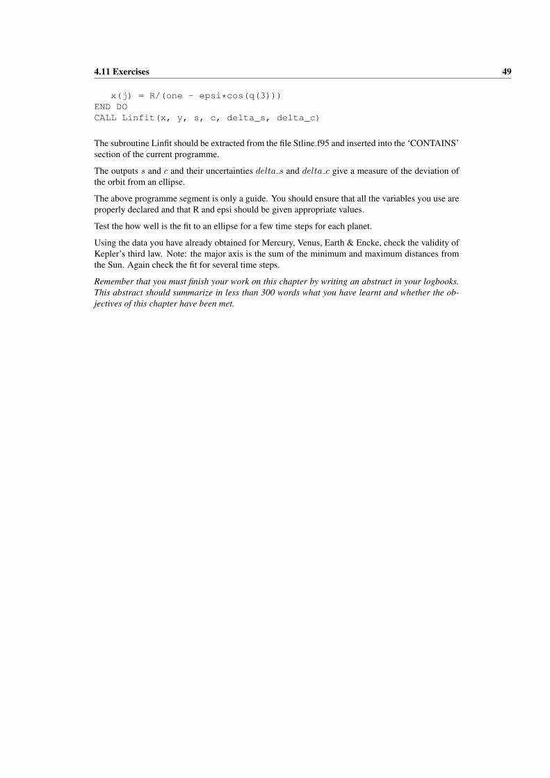
4.11 Exercises 49
x(j) = R/(one - epsi*cos(q(3)))END DOCALL Linfit(x, y, s, c, delta_s, delta_c)
The subroutine Linfit should be extracted from the file Stline.f95 and inserted into the ‘CONTAINS’section of the current programme.
The outputs s and c and their uncertainties delta s and delta c give a measure of the deviation ofthe orbit from an ellipse.
The above programme segment is only a guide. You should ensure that all the variables you use areproperly declared and that R and epsi should be given appropriate values.
Test the how well is the fit to an ellipse for a few time steps for each planet.
Using the data you have already obtained for Mercury, Venus, Earth & Encke, check the validity ofKepler’s third law. Note: the major axis is the sum of the minimum and maximum distances fromthe Sun. Again check the fit for several time steps.
Remember that you must finish your work on this chapter by writing an abstract in your logbooks.This abstract should summarize in less than 300 words what you have learnt and whether the ob-jectives of this chapter have been met.

4.11 Exercises 50