1

Efficient Learning of Image Super-resolution and CompressionArtifact Removal with Semi-local Gaussian Processes

Younghee Kwon, Kwang In Kim, James Tompkin, Jin Hyung Kim, and Christian Theobalt

Abstract—Improving the quality of degraded images is a key problem in image processing, but the breadth of the problem leads todomain-specific approaches for tasks such as super-resolution and compression artifact removal. Recent approaches have shown thata general approach is possible by learning application-specific models from examples; however, learning models sophisticated enoughto generate high-quality images is computationally expensive, and so specific per-application or per-dataset models are impractical. Tosolve this problem, we present an efficient semi-local approximation scheme to large-scale Gaussian processes. This allows efficientlearning of task-specific image enhancements from example images without reducing quality. As such, our algorithm can be easilycustomized to specific applications and datasets, and we show the efficiency and effectiveness of our approach across five domains:single-image super-resolution for scene, human face, and text images, and artifact removal in JPEG- and JPEG 2000-encoded images.

F

1 INTRODUCTION

Image degradation has many different causes, from lim-itations of the optical system, such as limited sensorresolution or lens defocus, to lossy image compression,creating block or ring artifacts. The removal of thesedegradations through image processing has been ap-proached in both application-specific and data-specificways, with different approaches for tasks such as super-resolution and compression artifact removal, and varia-tions for different data such as general scenes, faces, andtext images [1], [2], [3], [4], [5].

The inflexibility of application-specific models of im-age degradation has motivated methods which try togeneralize different image enhancement processes. Pre-vious successful approaches have integrated a prioriknowledge in a Bayesian framework in the form ofa generic prior on natural images, and have coupledthis with hand-designed application-specific parametricdegradation, or noise, models. However, typically thesenoise models are difficult to design, especially for non-Gaussian noise, which makes it difficult to adapt thesemethods to new applications and data.

Recent work has generalized further by learning afunction directly from example pairs of degraded andclean images. For instance, instead of parametric noisemodels, Kim and Kwong [6] apply non-parametric ker-nel ridge regression to map input degraded imagesto desired clean images, and so relieve the user from

• Y. Kwon is with Google Inc., 1600 Amphitheatre Pkwy, Mountain View,CA 94043, United States. youngheek@google.com

• K. I. Kim is with the School of Computing and Communications, LancasterUniversity, LA1 4WA, UK. k.kim@lancaster.ac.uk.

• J. Tompkin is with the School of Engineering and Applied Sciences,Harvard University, MA 02138, USA. jtompkin@seas.harvard.edu.

• J.-H. Kim is with Software Policy & Research Institute, 22Daewangpangyo-ro 712beon-gil, Bundang, Seongnam, Gyeonggi, Korea.jkim@kaist.ac.kr.

• C. Theobalt is with the Max-Planck-Institut fur Informatik, Campus E1-4,66123 Saarbrucken, Germany. theobalt@mpi-inf.mpg.de.

designing a noise model. However, applying modelssophisticated enough to generate high-quality imagesto application- and data-generic image enhancement ishindered by the high computational cost of learning, e.g.,[6] requires ≈36 hours of training.

Our major contribution1 is a method to remove thehigh computational complexity of training a conditionalnoise model, without affecting final enhancement qual-ity. Gaussian process (GP) regression is often used asit has powerful generalization capability that leads tobetter performance over simple nearest neighbor or lin-ear regressors; however, learning times are prohibitive,and sparse GP approximations require solving a difficultnon-linear optimization problem. We introduce a new ef-ficient semi-local approximation scheme to large-scale GPregression: Instead of time-consuming training and test-ing of a single GP model on a large dataset, a set of sparsemodels are constructed on-line such that the predictionat each test data point is made by the correspondingsparse GP approximating the underlying global model.We will demonstrate that during inference, i.e., enhance-ment, this method has a similar run-time complexity andperformance to general sparse models [6], [8], [9], [10].However, unlike existing models, by avoiding the time-consuming training stage, our approach facilitates easyadaptation to specific image degradation problems.

As a prior, we adopt the product of edge-perts frame-work [1]. This model adopts a sparsity prior (i.e., Lapla-cian) over the pair-wise joint distribution of waveletcoefficients which, overall, prefers simultaneous acti-vation of few coefficients in nearby scales and spatiallocations [1]. As a result, the dependencies betweenwavelet coefficients localized in frequency, space, andscale are effectively represented through product of expertstype factorization. With this framework and our semi-local GP regression, our algorithm allows building of animage enhancement system in 5 minutes from a set of ex-

1. A short version appeared in Proc. BMVC 2012 [7].

2

ample pairs of clean and degraded images, by deferringthe learning of a case specific conditional model to anonline approximation which, crucially, does not increasetesting time and retains enhancement quality.

We demonstrate the performance of our algorithmwith two specific applications across six datasets, one be-ing 500 images large: with single-image super-resolutionon general, face, and text images, and with artifactremoval in JPEG- and JPEG 2000-encoded images, whichhave block and ring artifacts respectively. Our exper-iments show that our algorithm outperforms state-of-the-art systems that are specific to each task ( [11], [12],[13], [14] for super-resolution, and [15], [16], [17], [18],[19], [20] for JPEG and JPEG 2000 artifact removal). Interms of inference or enhancement quality, our algorithmis on par with the state-of-the-art learning-based super-resolution algorithm of Kim and Kwon [6]; however, ourexperiments demonstrate that the significantly shortertraining time of our algorithm makes per-applicationand per-dataset image degradation learning practical.

2 RELATED WORK

Many image enhancement approaches estimate a func-tion that maps from the noise-affected image space to theclean image space. In general, a priori knowledge aboutnatural images can help, and, in principle, an imagemodel incorporating a generic prior of natural imagescan be applied to many enhancement applications withmodification of the noise model (or sometimes even witha Gaussian noise model).

The theory of projection onto convex sets (POCS) modelsprior knowledge as a set of convex constraints (e.g.,spatial smoothness, quantization constraints) [21] whichcast image enhancement into a POCS iteration frame-work [22], [23]. One direct way to use a priori knowledgeis to encode it into a distribution or an energy functional.Roth and Black describe a field of experts [3], where theprior is modeled as a Markov random field (MRF) withclique potentials learned from a set of natural images.

Laparra et al. [18] proposed a generic wavelet domainframework where the clean and noise image distribu-tions were estimated non-parametrically with supportvector regression (SVR). As a non-parametric model, thisapproach can be used in various image enhancement ap-plications. For Gaussian noise removal, this method out-performed one of the best image denoising methods —Gaussian scale mixtures (GSM) — with the perceptually-oriented structural similarity metric [24].

2.1 Learning-based single-image super-resolutionSingle-image super-resolution algorithms enlarge a sin-gle low-resolution image to high resolution. Existingapproaches are discussed in the literature [25], [26], [27];the most closely related approaches to our algorithmare example-based methods which identify a functionmapping a low-resolution image (or patch) to a high-resolution counterpart based on example pairs.

Freeman et al. proposed a nearest neighbor (NN)-based algorithm [14]. For each patch in the input low-resolution image, the corresponding high-resolution ex-ample patch is retrieved through NN-search that en-forces spatial consistency. Chang et al. [11] extendedthis idea by additionally introducing a reconstructionconstraint based on a manifold assumption.

In the context of regression estimation, Tappen etal. [28] performed multiple linear regressions on clus-tered example database and resolved the resulting mul-tiple candidate outputs by imposing a prior on naturalimages. Kim and Kwon generalized this idea by combin-ing sparse kernel ridge regression and adopting a prioron major edges [6]. Meanwhile, Yang et al. [12] adoptedthe idea of sparse coding in super-resolution. Here, a low-resolution input is represented as a sparse combinationof stored example inputs. The combination coefficientsare used to synthesize the corresponding outputs basedon the retrieved example outputs.

Gaussian processes (GP) have been used in variousimage enhancement problems. Tipping and Bishop [29]proposed applying a GP prior for multi-frame imagesuper-resolution while Liu [30], and He and Siu [13] usedGP regression for non-example-based image denoisingand super-resolution, respectively. Kim and Kwon [6]applied kernel ridge regression (KRR) that correspondsto non-Bayesian estimate of GP regression to example-based super-resolution. In the context of image super-resolution, KRR turned out to be easier to sparsify thansupport vector regression (SVR) and accordingly canpotentially lead to more practical algorithms [6].2

Our algorithm achieves better results than these pre-vious methods [11], [14], [28], and produces resultswhich are comparable to [6]; our approach also dra-matically enhanced applicability by two orders of mag-nitude faster training time. We also demonstrate thatour GP regression-based algorithm outperforms Yang etal.’s sparse coding-based algorithm which is anothercommonly used regression algorithm [12].

2.2 JPEG/JPEG 2000 compression artifact removalBlock-based discrete cosine transform (BDCT) codingis widely used to compress still images and video se-quences (e.g., JPEG/MPEG). However, at low bit rates,BDCT-encoded images can exhibit discontinuities atblock boundaries, known as block artifacts. JPEG 2000 re-places the BDCT stage with a discrete wavelet transform.This prevents block artifacts, but ringing artifacts maystill appear. Also, POCS has been successfully appliedto JPEG [22] and JPEG 2000 [23] image enhancement.

One of the best established methods for block artifactremoval is adaptive filtering with locally adjusted filterkernels to remove block edges while preserving imageedges [31]. A similar technique has also been applied

2. As shown in [6], optimizing SVR hyper-parameters for imagesuper-resolution leads to close to zero ε for ε-insensitive loss functionof SVR. Accordingly, the corresponding optimal solution is dense.

3

to the removal of ringing artifacts in the context oftrilateral filters [20]. Zhai et al. [19] proposed a block-shiftfiltering-based algorithm. For each pixel, the algorithmreconstructs a block encompassing that pixel based ona weighted combination of neighboring similar blocks.The overall result is a detail-preserving smoothing.

For learning approaches, Qiu [32] used a multi-layerPerceptron for JPEG deblocking while Lee et al. [33]proposed performing a piecewise linear regression inthe space of DCT coefficients and showed comparableresults to those of re-application of JPEG. Sun andCham [2] proposed a maximum a posteriori (MAP) frame-work, building upon fields of experts [3], which led toimproved performance over several existing methodsincluding those methods based on POCS and overcom-plete wavelet representations.

Finally, Nosratinia [15] proposed a surprisingand promising non-learning-based method called re-application of JPEG. This algorithm generates a set ofpixel-wise shifted versions of the input JPEG image, re-applies JPEG encoding to the shifted versions, and shiftsthem back to the original positions and averages. Whilesimple, re-application of JPEG demonstrates superiorperformance to algorithms based on nonlinear filtering,POCS, and overcomplete wavelets. An application toJPEG 2000 enhancement is also feasible [16].

In our experiments, we demonstrate that by exploitingrich information from a database of images, our algo-rithm generates much better images in terms of quantita-tive criteria and visual quality than existing algorithms.

3 THE IMAGE ENHANCEMENT ALGORITHM

We wish to generate an enhanced image from a degradedimage, with the aid of many example pairs of cleanand degraded images. First, we describe how we buildupon product of edge-perts (Edge-perts) and its prior [1]to learn the application- or dataset-specific conditionalnoise model. This learning relies upon Gaussian processregression to model the image enhancement process,and so second we motivate and explain the use of GPregression, specifically sparse GPs, and then explain ournew efficient semi-local GP approximation.

3.1 Our approachWe start with the Edge-perts approach, which providesa MAP framework in the decorrelated wavelet domain:

z∗ = arg maxz

(log p(z|z) + log p(z)) (1)

= arg minz

1

2‖z− z‖2 + σP (

∑j

wj [z]2j )αP

, (2)

where x is the latent clean image, x is the noisy inputimage, W[·] is the wavelet transform, z = W[x], andσP is the user-specified regularization hyper-parameter.The experts model parameters {wj} and αP ∈ [0, 1] areestimated by an expectation maximization algorithm [1].

A straightforward approach to apply the Edge-pertsframework to general image enhancement problems isto modify the noise model accordingly:

p(z|z) ∝∥∥z−W [I[W#(z)]

]∥∥2 , (3)

where I[·] is the degradation process of interest andW#(z) is the pre-image of z. However, Edge-perts as-sumes only Gaussian noise; for general noise, such as insuper-resolution applications, modeling the proper noisedistribution might be difficult or cumbersome. Further-more, general noise can be non-differentiable and evennon-continuous which leads to optimization difficulties.

Instead of a parametric noise model, we learn a condi-tional noise model from examples. However, naively im-plementing this step requires optimizing Eq. (3) throughlearning the degradation process, which may be com-putationally infeasible. To keep computations tractable,we bypass this complex optimization by decouplingthe conditional model learning and the optimization ofEq. (3): We introduce auxiliary reference variables s thatsummarize the outputs of the conditional model, andonly indirectly model the degradation process by encod-ing the information contained in the training examples.This model is computationally favorable and does notrequire the user to model the noise explicitly.

We penalize the cost functional:

E(z) =1

2‖z−W[s]‖2 + σP (

∑j

wj [z]2j )αP . (4)

The reference variable matrix s is constructed through re-gression. For each pixel location i in the input degradedimage x, a Gaussian process (GP) regressor receives adegraded patch (M × M ) centered at i, and producesestimates of an enhanced patch (N ×N ). GP regressionpredicts a Gaussian distribution: in our context, a meanpatch and a predictive variance patch. When N > 1,the output patch overlaps its spatial neighbors, and sofor each i in x, the contributions from N × N patchregressions constitute a set of candidates means fi, andcorresponding predictive variances vi. Then, si is aconvex combination of all overlapping patch candidatemeans fi ∈ RN and their confidences ci, where si = f>i ci,with [ci]j ≥ 0 and ‖ci‖L1

= 1. The confidence vectorci ∈ RN is calculated from the inverse of the predictivevariances vi ∈ RN of the candidates fi:

[ci]j = exp

(− [vi]jσC

)/ ∑k=1,...,N

exp

(− [vi]kσC

), (5)

where the scale parameter σC is fixed at 0.2. MinimizingEq. 4 and transforming from the wavelet basis thengenerates the enhanced image (as per [1]). Algorithm 1practically explains our framework in pseudocode.

Discussion. Generating several candidate means fi andpredictive variances vi across neighboring patches ag-gregates information from a wider image area thanfrom a single patch. Increasing patch size to aggregate

4

Algorithm 1: Image Enhancement (Super-resolution)Input : Low resolution input image L,

Training low/high res. image pairs X , Y .Output : Enhanced image S.Training: Build NN-search structure, e.g., KD-tree.

Testing :

Construct a bicubic upsampling B of L;

for each pixel pj in B doExtract a patch xj (centered at pj);Use semi-local GP regression to predictdistribution p(fj |Y) on output patch yj :1) Retrieve n-NNs (Cn) of xj from X ;2) Predict E[f(xj)] and V[f(xj)] from the labelsof Cn using Eq. (19);

endRe-arrange {E[f(xj)]} and {V[f(xj)]} foroverlapping patches so that for each pixel pi obtainssets of candidate means {fi} and correspondingvariances {vi};Build reference variable matrix s from {fi} and {vi};Minimize Eq. 4 and to find the enhanced image S.

more information is possible, but in preliminary ex-periments we found that the difficulty in learning inhigher-dimensional spaces resulted in worse predictionthan our patches (e.g., 7× 7 for 2× magnification super-resolution). Compared to single-pixel-output regression,patch-valued regression produced 0.6dB PSNR increasein super-resolution experiments (as per [6]).

Unlike elegant fully Bayesian image models (e.g., [4]),an intuitive probabilistic interpretation of the image en-hancement process is no longer possible: the predictivedistribution of a GP is a posterior distribution that is con-ditioned on the degraded input patches. Since this con-ditional model is not generative, sampling a degradedimage is not directly possible. This functionality is notrequired for image enhancement applications. Using thelocal posterior distribution as a surrogate noise modelhas been well established in speech recognition [34]and similar strategies have been recently used in imageenhancement as well [5], [28]. In general, Eq. 4 couldbe regarded as a regularization framework which tradesbetween regularity enforcement in the wavelet domainand deviation from the reference variables {si}.

3.2 RegressionThe underlying idea for using GP regression is its pow-erful generalization capability. For instance, in classicalexample-based super-resolution applications, a typicalchoice for the conditional model is NN-based estimation[14], [26], [35]. However, from the general regressionperspective, NN regression can be improved since itoverfits to the data, i.e., we obtain a function whichfits the training data perfectly but cannot generalize to

new data. GP regression has powerful regularizationcapability which avoids overfitting and leads to a bettergeneralization than NN regression (See Fig. 1, Sec. 4.1,and supplementary material for comparison with NNapproaches [11], [14]). GP regression is much more flex-ible than simple linear regression, which fails when theproblem is highly non-linear (Fig. 1). Furthermore, inour super-resolution experiments, we demonstrate thatour algorithm outperforms Yang et al.’s sparse codingregression choice [12].

We review basic GP regression in Section 3.2.1, be-fore reviewing more efficient sparse GP approxima-tions which requires optimizing inducing variables (Sec-tion 3.2.2). Section 3.2.3 introduces our new GP approx-imation which bypasses completely the inducing vari-ables optimization and therefore facilitates fast training.

3.2.1 Basic Gaussian process regressionSuppose a set of data points (in our case, vectorizedpatches) X = {x1, . . . ,xl} ⊂ RM2

and their correspond-ing labels Y = {y1, . . . ,yl} ⊂ RN2

. We adopt a Gaussiannoise model with mean 0 and the covariance matrix σ2I:

yi = f(xi) + ε, where ε ∼ N (0, σ2I), (6)

where N (µ,Σ) is the probability density of the Gaus-sian random variable with mean µ and covariance Σ,and f : RM2 7→ RN2

is the underlying latent func-tion. Then, a zero-mean Gaussian process (GP) prioris placed over f , which for a given set of test pointsX∗ = {x∗(1), . . . ,x∗(l′)} is realized as [36]:3

p(f∗, f) = N

(0,

[Kf ,f Kf ,∗

K∗,f K∗,∗

]), (7)

where the subscripts f and ∗ represent indexing acrosstraining and testing data points, respectively (e.g., f =[f(x1), . . . , f(xl)]

>, f∗ = [f(x∗(1)), . . . , f(x∗(l′))]>, and

[(K∗,f )(i,j)]l′,l = k(x∗(i),xj)). While any positive definitefunction can be used as the covariance function k, weadopt the standard Gaussian kernel:

k(x,y) = exp(−b‖x− y‖2

).

Combining (6) and (7), the joint distribution of p(f∗,Y):

p(f∗,Y) = N

(0,

[Kf ,f + σ2I Kf ,∗

K∗,f K∗,∗

]), (8)

from which, the predictive distribution (for the j-thoutput dimension; index j in f∗ is omitted) is constructedby conditioning f∗ on the labels Y :

p(f∗|Y) =N(K∗,f (Kf ,f + σ2I)−1Y[:,j],

K∗,∗ −K∗,f (Kf ,f + σ2I)−1Kf ,∗), (9)

where Y = [y>1 , . . . ,y>l ]> and A[:,j] is the j-th column of

the matrix A. For the simplicity of exposition, we adopt a

3. For computational convenience, we treat each output indepen-dently and identically. For notational convenience, we omit condition-ing on input variables.

5

slight misuse of notations and summarize the predictivedistribution (9) across every output dimensions as:

p(f∗|Y) =N(K∗,f (Kf ,f + σ2I)−1Y,

K∗,∗ −K∗,f (Kf ,f + σ2I)−1Kf ,∗), (10)

where each output dimension shares the covariance.The diagonal terms of the covariance matrix (predic-

tive variances) in the predictive distribution (9) representthe uncertainty of regression output, while off-diagonalterms represent the dependency between variables.

While GP regression has been shown to be compet-itive on a wide range of small-scale applications, itsapplication to large-scale problems is limited due toits unfavorable scaling behavior: The training (i.e., thecalculation of Kf ,f and the corresponding regularizedinversion) takes O(Ml2 + l3) time, while for a giventest point, testing time complexity is O(Ml + lN) andO(Ml + l2) for the mean and the predictive variance,respectively (see [36] for details).

3.2.2 Sparse Gaussian processesA standard approximate approach to overcome the un-favorable scaling behavior of GPs is to introduce asmall set of inducing variables fU = {f(u1), . . . , f(um)}(corresponding to inducing inputs U = {u1, . . . ,um})through which the conditional independence of f∗ and fis assumed in the approximation of the joint prior (seethe unified framework of [10]):

p(f∗, f) ≈ q(f∗, f) =

∫q(f∗|fU )q(f |fU )p(fU )dfU . (11)

The training conditional q(f |fU ) is approximated subse-quently. This leads to a set of approximations which arereferred to as sparse GPs where the inference is carriedout through U summarizing the entire training set X [8],[9], [37]. For instance, Seeger et al. [37] proposed anapproximate prior:

q(f∗, f) = N

(0,

[QUf ,f QUf ,∗QU∗,f K∗,∗

]), (12)

where QUr,s = Kr,uK−1u,uKu,s and u represents indexingacross U . The corresponding predictive distribution is:

q(f∗|Y) =N(QU∗,f (Q

Uf ,f + σ2I)−1Y,

K∗,∗ −QU∗,f (QUf ,f + σ2I)−1QUf ,∗

). (13)

With this prior, the predictive mean is obtained as alinear combination of evaluations of m basis functions{k(u1, ·), . . . , k(um, ·)} (explaining the name sparse GPs).The time complexity of calculating the predictive distri-bution becomes O(Mlm + lm2) off-line plus O(Mm +mN +m2) per test point.

Once we identify the inducing inputs U , they are fixedthroughout the entire test set. The problem is then castinto an optimization where one constructs U based on acertain measure of approximation quality (e.g., marginallikelihood and information gain; see [8], [9], [36], [37]

for more examples and details). The performance of asparse approximation depends heavily on the inducinginputs U . However, usually the corresponding optimiza-tion problem is non-convex and so requires a non-linearoptimization which is not easy to solve.

3.2.3 Semi-local approximation of Gaussian processesOur approach is fundamentally different from exist-ing algorithms, and bypasses non-linear optimizationthrough inducing inputs U using a simple heuristic:Instead of sharing U for all test data points, we sim-ply approximate the inducing variables as the nearestneighbors (NNs) of each test input.

We build a specially-tailored sparse GP for each testinput x∗, i.e., U ≡ U∗ is chosen depending on x∗ — thecorresponding GP model is constructed only when it ispresented with a test point x∗. An important advantageof this on-line approach is that, in general, it enables moreflexible approximations than existing off-line approaches.

Furthermore, it leads to an extremely simple butpowerful strategy for identifying U∗: If we introduce aMarkov assumption on {f∗, f}, (f∗ ≡ f(x∗)):

p(f∗|f ,B(f∗)) ≈ q(f∗|B(f∗)), (14)

where B(f∗) is the values of f for inputs in the domainneighborhoods B(x∗) ⊂ X of x∗, then the correspondingconditional independence of f∗ and f given B(f∗) makesB(x∗) a valid candidate for U∗, i.e., the approximation(11) becomes exact once we use B(x∗) for U∗. Now,applying Eq. 14 to Eq. 13 we obtain QUr,s specified asQBr,s = Kr,bK−1b,bKu,s with b indexing across B(x∗):

q(f∗|Y) =N(QB∗,f (Q

Bf ,f + σ2I)−1Y,

K∗,∗ −QB∗,f (QBf ,f + σ2I)−1QBf ,∗

)=N

(σ−2K∗,bΣBKb,fY,

K∗,∗ −QB∗,∗ + K∗,bΣBKb,∗), (15)

where ΣB =(σ−2Kb,fKf ,b + Kb,b

)−1 and the sec-ond equality is obtained by applying Sherman-Morrison-Woodbury formula.

This new approximation dramatically reduces thecomputation time during training as we only need tobuild a data structure for NN-search to identify B(f∗).During prediction, it takes O(Mlm+ lm2) time for eachtest point with m = |B(f∗)|, which includes the timespent building a model. However, for large l (≈ 2 ∗ 105

in current applications), this might still be impractical.Hence, the second step of our approximation is ob-

tained by introducing an additional Markov-like as-sumption on the observations Y :

p(f∗|Y,B1(y∗)) ≈ q(f∗|B1(y∗)), (16)

where B1(y∗) denotes the observed training target valuesin the domain neighborhood B1(x∗) of x∗. In general,neither (14) nor (16) is stronger than the other sinceneither is implied by the other — only when the noise

6

level is zero do the two assumptions become equiv-alent. However, practically, (16) can be regarded as astronger assumption than (14), since (16) implies thatgiven B1(y∗), all the remaining training data points areirrelevant in making predictions of f∗, which is not thecase for (14). Accordingly, we set B1(x∗) much widerthan B(x∗) (i.e., B1(x∗) ⊃ B(x∗)). This guarantees thatthe resulting GPs are non-locally regularized. In Sec. 5,for the interested reader, we discuss the motivationbehind this second approximation step, which is basedon analysis of the large-scale behavior of full GPs.

In practice, we choose m and n-nearest neighborsCn(x∗)(Cm(x∗) ⊂ Cn(x∗) ⊂ X ) of x∗, instead of B(f∗)and B1(y∗), such that prediction is performed based onn data points summarized by m inducing inputs. Now,applying Eq. 16 to Eq. 15 in this context, we obtain:

q(f∗|YC) = N(σ−2K∗,bΣBCKb,cYC),

K∗,∗ −QB∗,∗ + K∗,bΣBCKb,∗), (17)

where in a compact notation YC and YC representthe subset of Y and the rows of Y, respectively cor-responding to the elements of Cn(x∗) ⊂ X , ΣBC =(σ−2Kb,cKc,b + Kb,b

)−1, and c represents indexingacross Cn(x∗). The sizes of the neighborhoods m and nare decided based on prescribed computational complex-ity requirement (Sec. 4).

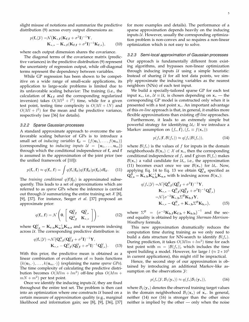
We refer to this new approximation as semi-local GP.With the same number of inducing inputs, this input-dependent selection should, in general, provide moreflexibility than standard sparse methods because theinducing variables are specifically tailored to each testdata point. As shown in Fig. 1, for smaller numbers ofinducing inputs our semi-local GPs perform especiallybetter than sparse methods, which use relatively largenumbers of carefully chosen inducing inputs.

Furthermore, given hyper-parameters, the only train-ing component for semi-local GPs is to build a datastructure for NN-search, and so off-line processing isvery fast. Therefore, the algorithm is very flexible as thesystem can be easily adapted to the distribution of aspecific (non-generic) class of images (see Sec. 4.1).

Discussion. The Markov model used in the first stepof approximation (Eq. 14) has proven to be effective inmany different applications. However, we exploit theMarkov assumptions only in the approximation of theprior through its factorization and the marginalizationover fU in Eq. 11. Accordingly, although the resultingsparse model can represent only local variations aroundx∗, the corresponding prediction takes into account theentire data set through the dependency between f andfU∗ (see Eq. 11). This implies that for each test variablef∗, the corresponding joint distribution q(f∗, f) fits intothe approximation (Eq. 12) and it is a valid probabilisticapproximation of the full GP. In particular, no overfittingoccurs since the model is globally regularized. This is incontrast to the moving least-squares algorithm which is

50100 300 500 750 1000−12

−11

−10

−9

−8

KL

dive

rgen

ce

50100 300 500 750 10000.8

1

1.2

1.4

1.6

1.8

# inducing inputs in sparse GP

Incr

. PS

NR

s

sparse GPsemi−local GPNNlinear

Fig. 1: Approximation accuracies of sparse GPs andsemi-local GPs wrt. full GP for the super-resolutionexperiment data points. Top: The Kullback-Leibler diver-gences from full GPs of the predictive distributions ofapproximate GPs, plotted against m′ sparse GP inducinginputs. To compare, we use only 20, 000 data points totrain all models, sampled from a large training set of200,000. For each m′, a semi-local GP was trained, withnumber of inducing inputs m and local training datapoints n such that the time complexity of test pointprediction roughly matches ((m′)2 ≈ m2n). Experimentswere repeated ten times with randomly selected trainingdata sets. Error bar lengths are 2× std. dev. Bottom:Average PSNR increase from bicubic resampling, mea-sured from final super-resolution results. For compari-son, we replace our regression by linear regression andNN regression. The inducing inputs were optimized bymaximizing the marginal likelihood p(f∗|u) [8].

not directly related to any global regularization.Theoretically, one drawback of our on-line model is

that it does not correspond to any consistent global GPframework: In our model, the prior is defined throughthe inducing variables (Eq. 11) that depend on eachtest input. Since, in general, the Gaussian property ofmarginal distributions q(f∗, f) does not imply the Gaus-sian property of the corresponding joint distribution, itmay not be possible to construct a Gaussian joint priorq(f∗, f) over the entire set of potential testing points f∗.

A direct consequence of this inconsistency is that,since there is no globally defined covariance function,no prediction can be made for off-diagonal elements ofthe predictive covariance, which represents the depen-dency between predictions.4 However, this is not a majorconcern as we only use the means and variances of indi-vidual predictions {p(f∗|Y)}, which are valid probabilitydistributions (i.e., p(f∗|Y) is a fully Bayesian prediction).

4. Snelson and Ghahramani proposed an inconsistent GP approxi-mation [38] where the training data are pre-partitioned during traininginto a set of clusters which constitute input-dependent inducing inputs.

7

3.3 Noise modelThere are two sources of uncertainty in making predic-tions with GPs [39]. One is the fact that, in general, thetest input may deviate from the training inputs (U1).The other is the noise in the data (U2): Due to theill-posed nature of the problem, even if the test inputx∗ exactly matches one of the training inputs (say xi),the corresponding training output yi might not be theunderlying ground truth output f(x∗). In the currentcontext of GP regression, U1 and U2 uncertainties areindependently modeled with the noise parameter (σ2)and the kernel parameter (b), respectively. This clearseparation is due to the use of an i.i.d. Gaussian noisemodel (Eq. 6) which is important because it leads to ananalytical model for predictive distribution (Eq. 9).

In general, the noise (U2) is correlated and depends onthe input (and so on U1). However, sophisticated noisemodels which reflect this dependency may lead to non-analytic predictive distributions and so are not computa-tionally favorable for image enhancement applications.

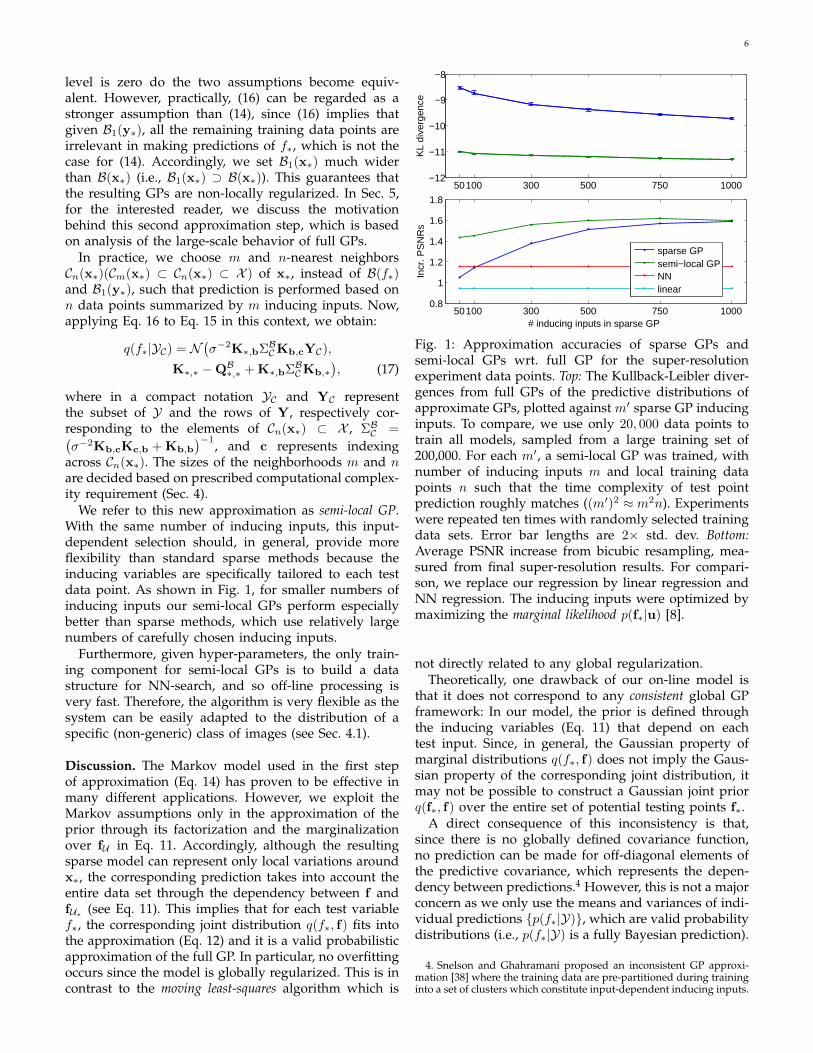
We present a simple noise model which exploits thedependency between these two sources of uncertainty.Our scheme considers the empirically-observed correla-tion between two quantities which are related to U1 andU2. The first quantity P1 is the average distance from atest input to its nearest training inputs, which representsU1. The second quantity P2 is the average distanceamong the corresponding retrieved training outputs.This is not directly related to U2; however, when P1is zero, P2 should correspond to the standard deviationof the output conditioned on an input and, accordingly,be an empirical estimate of the noise level U2.

By construction, P1 and P2 are mildly correlated: IfP1 is small, the corresponding training inputs should beclose to each other and so P2 tends to be small. However,Fig. 2 shows there are cases where the correlation ismuch stronger: when P1 is very small, P1 and P2 areespecially strongly correlated (e.g., P1 < 0.005, whenthe test input is very close to some training inputs). AsP1 increases, the correlation becomes weaker and even-tually disappears. This observation led us to conjecturethat U2 is correlated to U1 especially when U1 is small.

We validate this conjecture by implementing it into ournoise model. Our semi-local GP model is adaptive in thesense that the model itself depends on each test input.Naturally, the noise parameter σ2 can also be adaptedto each test input x∗ (and its distances to the storedtraining inputs). For computational efficiency, we stilluse a Gaussian noise model but adapt it to the localdensity at the point of evaluation. Eq. 17 then becomes:

q(f∗|YC) =N(K∗,b(ΣBC )′Kb,cΓYC ,

K∗,∗ −QB∗,∗ + K∗,b(ΣBC )′Kb,∗), (18)

where

(ΣBC )′ = (Kb,cΓKc,b + Kb,b)−1, (19)

Γ =diag [Nc exp (−Ndbd)] + σ−2I, (20)

0.005 0.01 0.015 0.02 0.025 0.030.02

0.04

0.06

0.08

0.1

0.12

0.14

0.16

P1

P2

Fig. 2: Variation of P2 as a function P1 in super-resolution experiments (see text for P1 and P2 descrip-tions): For each test input, we select 10 nearest neighborsand calculate the corresponding P1 and P2 values.

d is a vector containing the squared distances betweenx∗ and the elements of Cn(x∗), Nc and Nd are the hyper-parameters, and diag[·] is an operator which converts avector into a diagonal matrix.

From the regularization perspective, the noise vari-ance σ2 is the parameter controlling the contributionof training error and the global regularization term. Anintuitive explanation of our noise model is that when thegiven input is sufficiently close to the training data, werely more on data than on regularization. Furthermore,within the set of training data points, we emphasizemore the data points which are closer to the test input.The computational complexity of this model is the sameas that of the uniform noise model (17). However, thismodel resulted in on average 0.08 improvement of PSNRvalues in our super-resolution experiments.

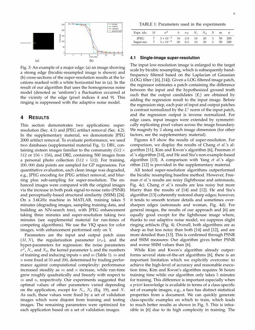
Discussion. We observe that most easy test points withsmall P1 values lie at major edges (see supplementarymaterial for examples). Typically, the major edges showclean and strong change of pixel values and do notcontain complex textures. Intuitively, for those patterns,the noise level must be low, i.e., the desired outputshould be less uncertain given the input. This explainsa strong correlation between P1 and P2 for small P1values. The role of our adaptive noise model (18) is thento regularize less for those patterns lying at major edges.

A visually noticeable consequence is that ringing ar-tifacts are significantly reduced. Typically the results ofregularized regression show a certain fluctuation whenthere is an abrupt and significant change of the signal tocompensate the resulting loss of smoothness. By placingmore emphasis on observed data than the regularizer,we can effectively suppress these regularization artifactswhich appear as ringing artifacts (Figure 3). Kim andKwon [6] adopted a post-processing step to explicitlyremove the ringing artifact, which is not necessary whenwe use an adaptive noise model.

8

0 2 4 6 8 10 12 14

0

50

100

150

200

250

Pixel index

Pix

el v

alue

bicubicuniformadaptiveground truth

(a) (b)

Fig. 3: An example of a major edge: (a) an image showinga strong edge (bicubic-resampled image is shown) and(b) cross-sections of the super-resolution results at the lo-cations marked with a white horizontal bar in (a). In theresult of our algorithm that uses the homogeneous noisemodel (denoted as ‘uniform’) a fluctuation occurred atthe vicinity of the edge (pixel indices 4 and 9). Thisringing is suppressed with the adaptive noise model.

4 RESULTS

This section demonstrates two applications: super-resolution (Sec. 4.1) and JPEG artifact removal (Sec. 4.2).In the supplementary material, we demonstrate JPEG2000 artifact removal. To evaluate performance, we usedtwo databases (supplemental material Fig. 1): DB1, con-taining sixteen images familiar to the community (512×512 or 256× 256), and DB2, containing 500 images froma personal photo collection (512 × 512). For training,200, 000 data points are sampled for GP regressions. Forquantitative evaluation, each clean image was degraded,e.g., JPEG encoding for JPEG artifact removal, and blur-ring plus sub-sampling for super-resolution. The en-hanced images were compared with the original imagesvia the increase in both peak signal-to-noise ratio (PSNR)and perceptually-based structural similarity (SSIM) [24].On a 3.6GHz machine in MATLAB, training takes 5minutes (degrading images, sampling training data, andbuilding an NN-search tree), with JPEG enhancementtaking three minutes and super-resolution taking twominutes (see supplemental material for run-times ofcompeting algorithms). We use the YIQ space for colorimages, with enhancement performed only on Y.

Parameters are the input and output patch sizes(M,N ), the regularization parameter (σP ), and thehyper-parameters for regression: the noise parametersσ2, Nc, and Nd, the kernel parameter b, and the numbersof training and inducing inputs n and m (Table 1). m andn were fixed at 50 and 200, determined by trading perfor-mance against computational complexity: performanceincreased steadily as m and n increase, while run-timegrew roughly quadratically and linearly with respect tom and n, respectively. Our experiments suggested thatoptimal values of other parameters varied dependingon the application, except for Nc, Nd (Eq. 19), and N .As such, these values were fixed by a set of validationimages which were disjoint from training and testingimages. The remaining parameters were optimized foreach application based on a set of validation images.

TABLE 1: Parameters used in the experiments

Expr. idx. M σ2 b σP Nc Nd N m n

JPEG 7 5 ∗ 10−3 10 2.0 10 20 5 50 200Super-res. 7 5 ∗ 10−8 20 0.5 10 20 5 50 200

4.1 Single-image super-resolution

The input low-resolution image is enlarged to the targetscale by bicubic resampling, which is subsequently band-frequency filtered based on the Laplacian of Gaussian(LOG) filter ( [6], [14]). Given a LOG filtered image patch,the regressor estimates a patch containing the differencebetween the input and the hypothesized ground truthsuch that the output candidates {fi} are obtained byadding the regression result to the input image. Beforethe regression step, each pair of input and output patchesis contrast normalized by the L1 norm of the input patch,and the regression output is inverse normalized. Foredge cases, input images were extended by symmetri-cally replicating pixel values across the image boundary.We magnify by 2 along each image dimension (for otherfactors, see the supplementary material).

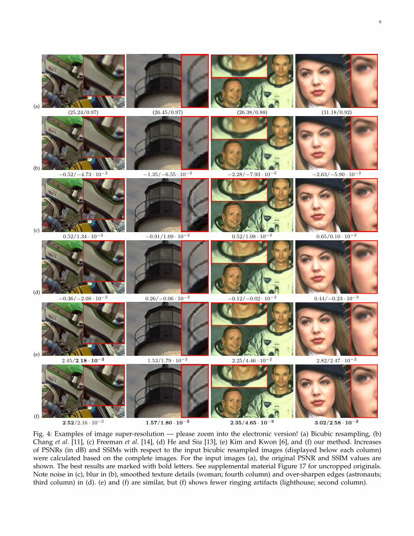
Figures 4-5 show the results of super-resolution. Forcomparison, we display the results of Chang et al.’s al-gorithm [11], Kim and Kwon’s algorithm [6], Freeman etal.’s algorithm [14], and He and Siu’s non-example-basedalgorithm [13]. A comparison with Yang et al.’s algo-rithm [12] is provided in the supplementary material.

All tested super-resolution algorithms outperformedthe bicubic resampling baseline method. However, Free-man et al.’s results are noisy (lighthouse and astronauts,Fig. 4c). Chang et al.’s results are less noisy but moreblurry than the results of [14] and [12]. He and Siu’salgorithm [13] coherently restored sharp edges; however,it tends to smooth texture details and sometimes over-sharpen edges (astronauts and woman, Fig. 4d). Forgeneral images, the results of our approach and [6] areequally good except for the lighthouse image where,thanks to our adaptive noise model, we suppress slightringing artifacts (Fig. 4). Overall, both algorithms are assharp as but less noisy than both [14] and [12], and aremore detailed than [13]. This is confirmed through PSNRand SSIM measures: Our algorithm gives better PSNRand worse SSIM values than [6].

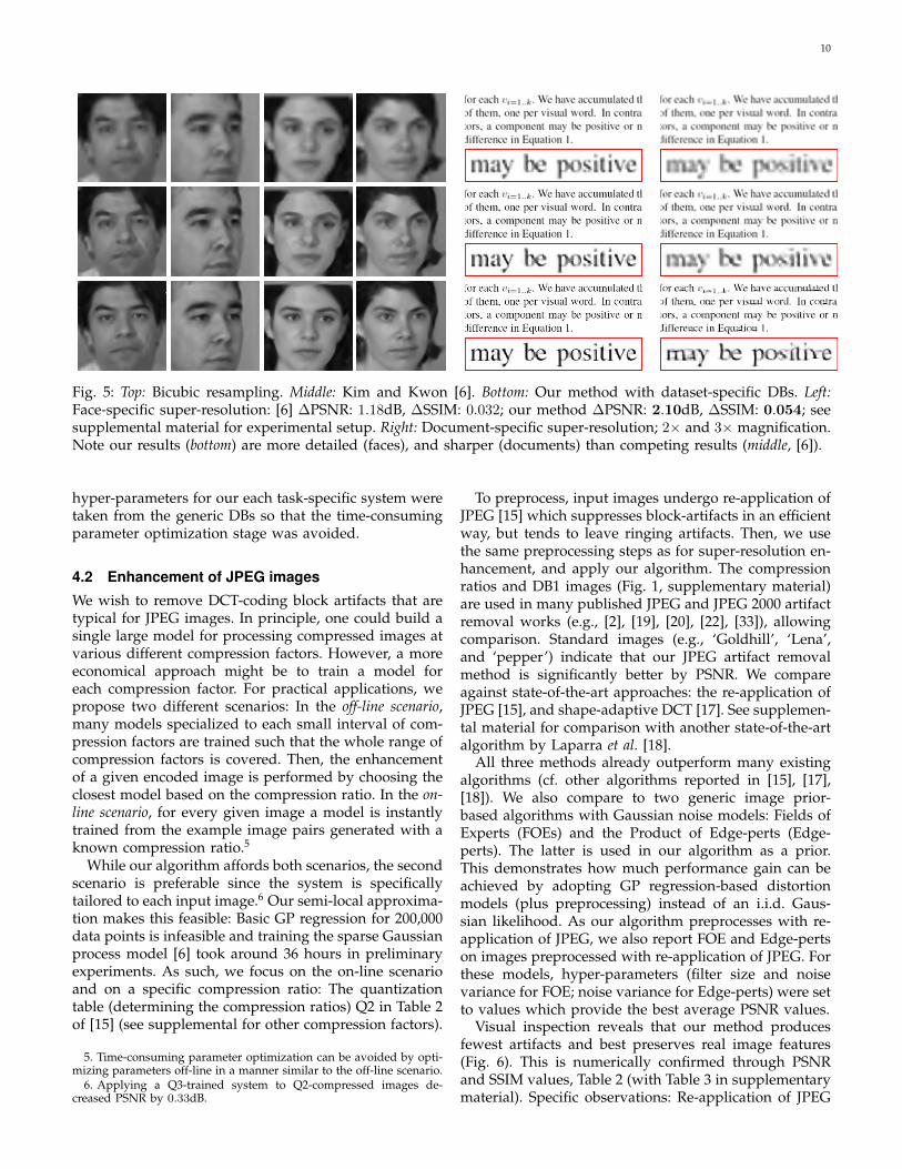
While Kim and Kwon’s algorithm already outper-forms several state-of-the-art algorithms [6], there is animportant limitation which we explicitly overcome: toachieve the high-level of accuracy and reasonable execu-tion time, Kim and Kwon’s algorithm requires 36 hourstraining time while our algorithm only takes 5 minutesfor training. This difference is important especially whena priori knowledge is available in terms of a class-specificset of example images, e.g., a face has distinct statisticalproperties from a document. We can quickly generateclass-specific examples on which to train, which leadsto much better results as shown in Fig. 5. This is infea-sible in [6] due to its high complexity in training. The

9

(a)(25.24/0.97) (26.45/0.97) (26.38/0.88) (31.18/0.92)

(b)−0.52/−4.73 · 10−2 −1.35/−6.55 · 10−2 −2.28/−7.93 · 10−2 −2.63/−5.90 · 10−2

(c)0.52/1.34 · 10−2 −0.91/1.09 · 10−2 0.52/1.08 · 10−2 0.65/0.10 · 10−2

(d)−0.36/−2.08 · 10−2 0.26/−0.06 · 10−2 −0.12/−0.02 · 10−2 0.44/−0.23 · 10−2

(e)2.45/2.18 · 10−2 1.53/1.79 · 10−2 2.25/4.46 · 10−2 2.82/2.47 · 10−2

(f)2.52/2.16 · 10−2 1.57/1.80 · 10−2 2.35/4.65 · 10−2 3.02/2.58 · 10−2

Fig. 4: Examples of image super-resolution — please zoom into the electronic version! (a) Bicubic resampling, (b)Chang et al. [11], (c) Freeman et al. [14], (d) He and Siu [13], (e) Kim and Kwon [6], and (f) our method. Increasesof PSNRs (in dB) and SSIMs with respect to the input bicubic resampled images (displayed below each column)were calculated based on the complete images. For the input images (a), the original PSNR and SSIM values areshown. The best results are marked with bold letters. See supplemental material Figure 17 for uncropped originals.Note noise in (c), blur in (b), smoothed texture details (woman; fourth column) and over-sharpen edges (astronauts;third column) in (d). (e) and (f) are similar, but (f) shows fewer ringing artifacts (lighthouse; second column).

10

Fig. 5: Top: Bicubic resampling. Middle: Kim and Kwon [6]. Bottom: Our method with dataset-specific DBs. Left:Face-specific super-resolution: [6] ∆PSNR: 1.18dB, ∆SSIM: 0.032; our method ∆PSNR: 2.10dB, ∆SSIM: 0.054; seesupplemental material for experimental setup. Right: Document-specific super-resolution; 2× and 3× magnification.Note our results (bottom) are more detailed (faces), and sharper (documents) than competing results (middle, [6]).

hyper-parameters for our each task-specific system weretaken from the generic DBs so that the time-consumingparameter optimization stage was avoided.

4.2 Enhancement of JPEG images

We wish to remove DCT-coding block artifacts that aretypical for JPEG images. In principle, one could build asingle large model for processing compressed images atvarious different compression factors. However, a moreeconomical approach might be to train a model foreach compression factor. For practical applications, wepropose two different scenarios: In the off-line scenario,many models specialized to each small interval of com-pression factors are trained such that the whole range ofcompression factors is covered. Then, the enhancementof a given encoded image is performed by choosing theclosest model based on the compression ratio. In the on-line scenario, for every given image a model is instantlytrained from the example image pairs generated with aknown compression ratio.5

While our algorithm affords both scenarios, the secondscenario is preferable since the system is specificallytailored to each input image.6 Our semi-local approxima-tion makes this feasible: Basic GP regression for 200,000data points is infeasible and training the sparse Gaussianprocess model [6] took around 36 hours in preliminaryexperiments. As such, we focus on the on-line scenarioand on a specific compression ratio: The quantizationtable (determining the compression ratios) Q2 in Table 2of [15] (see supplemental for other compression factors).

5. Time-consuming parameter optimization can be avoided by opti-mizing parameters off-line in a manner similar to the off-line scenario.

6. Applying a Q3-trained system to Q2-compressed images de-creased PSNR by 0.33dB.

To preprocess, input images undergo re-application ofJPEG [15] which suppresses block-artifacts in an efficientway, but tends to leave ringing artifacts. Then, we usethe same preprocessing steps as for super-resolution en-hancement, and apply our algorithm. The compressionratios and DB1 images (Fig. 1, supplementary material)are used in many published JPEG and JPEG 2000 artifactremoval works (e.g., [2], [19], [20], [22], [33]), allowingcomparison. Standard images (e.g., ‘Goldhill’, ‘Lena’,and ‘pepper’) indicate that our JPEG artifact removalmethod is significantly better by PSNR. We compareagainst state-of-the-art approaches: the re-application ofJPEG [15], and shape-adaptive DCT [17]. See supplemen-tal material for comparison with another state-of-the-artalgorithm by Laparra et al. [18].

All three methods already outperform many existingalgorithms (cf. other algorithms reported in [15], [17],[18]). We also compare to two generic image prior-based algorithms with Gaussian noise models: Fields ofExperts (FOEs) and the Product of Edge-perts (Edge-perts). The latter is used in our algorithm as a prior.This demonstrates how much performance gain can beachieved by adopting GP regression-based distortionmodels (plus preprocessing) instead of an i.i.d. Gaus-sian likelihood. As our algorithm preprocesses with re-application of JPEG, we also report FOE and Edge-pertson images preprocessed with re-application of JPEG. Forthese models, hyper-parameters (filter size and noisevariance for FOE; noise variance for Edge-perts) were setto values which provide the best average PSNR values.

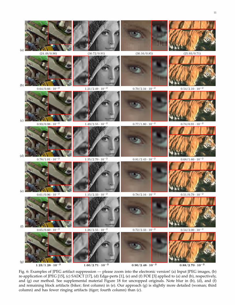
Visual inspection reveals that our method producesfewest artifacts and best preserves real image features(Fig. 6). This is numerically confirmed through PSNRand SSIM values, Table 2 (with Table 3 in supplementarymaterial). Specific observations: Re-application of JPEG

11

(a)(24.49/0.90) (30.72/0.91) (30.16/0.85) (25.93/0.71)

(b)0.64/0.66 · 10−2 1.21/2.49 · 10−2 0.70/2.34 · 10−2 0.54/2.10 · 10−2

(c)0.93/0.98 · 10−2 1.49/2.55 · 10−2 0.77/1.80 · 10−2 0.74/0.91 · 10−2

(d)0.78/1.01 · 10−2 1.35/2.70 · 10−2 0.81/2.43 · 10−2 0.68/1.60 · 10−2

(e)0.61/0.96 · 10−2 1.15/2.33 · 10−2 0.78/2.16 · 10−2 0.51/0.79 · 10−2

(f)0.65/0.60 · 10−2 1.26/2.55 · 10−2 0.72/2.33 · 10−2 0.54/2.00 · 10−2

(g)1.23/1.28 · 10−2 1.60/2.71 · 10−2 0.90/2.48 · 10−2 0.88/2.70 · 10−2

Fig. 6: Examples of JPEG artifact suppression — please zoom into the electronic version! (a) Input JPEG images, (b)re-application of JPEG [15], (c) SADCT [17], (d) Edge-perts [1], (e) and (f) FOE [3] applied to (a) and (b), respectively,and (g) our method. See supplemental material Figure 18 for uncropped originals. Note blur in (b), (d), and (f)and remaining block artifacts (biker; first column) in (e). Our approach (g) is slightly more detailed (woman; thirdcolumn) and has fewer ringing artifacts (tiger; fourth column) than (c).

12

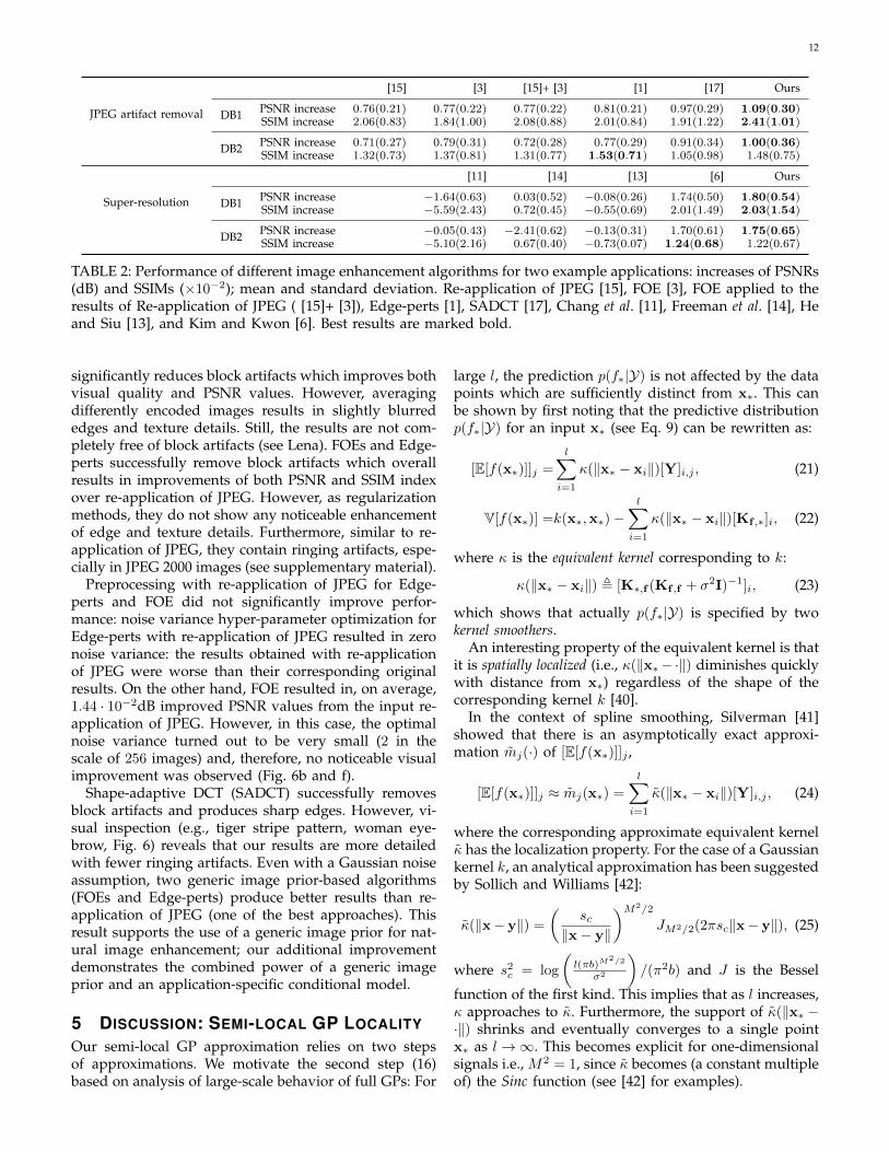
JPEG artifact removal

[15] [3] [15]+ [3] [1] [17] Ours

DB1 PSNR increase 0.76(0.21) 0.77(0.22) 0.77(0.22) 0.81(0.21) 0.97(0.29) 1.09(0.30)SSIM increase 2.06(0.83) 1.84(1.00) 2.08(0.88) 2.01(0.84) 1.91(1.22) 2.41(1.01)

DB2 PSNR increase 0.71(0.27) 0.79(0.31) 0.72(0.28) 0.77(0.29) 0.91(0.34) 1.00(0.36)SSIM increase 1.32(0.73) 1.37(0.81) 1.31(0.77) 1.53(0.71) 1.05(0.98) 1.48(0.75)

Super-resolution

[11] [14] [13] [6] Ours

DB1 PSNR increase −1.64(0.63) 0.03(0.52) −0.08(0.26) 1.74(0.50) 1.80(0.54)SSIM increase −5.59(2.43) 0.72(0.45) −0.55(0.69) 2.01(1.49) 2.03(1.54)

DB2 PSNR increase −0.05(0.43) −2.41(0.62) −0.13(0.31) 1.70(0.61) 1.75(0.65)SSIM increase −5.10(2.16) 0.67(0.40) −0.73(0.07) 1.24(0.68) 1.22(0.67)

TABLE 2: Performance of different image enhancement algorithms for two example applications: increases of PSNRs(dB) and SSIMs (×10−2); mean and standard deviation. Re-application of JPEG [15], FOE [3], FOE applied to theresults of Re-application of JPEG ( [15]+ [3]), Edge-perts [1], SADCT [17], Chang et al. [11], Freeman et al. [14], Heand Siu [13], and Kim and Kwon [6]. Best results are marked bold.

significantly reduces block artifacts which improves bothvisual quality and PSNR values. However, averagingdifferently encoded images results in slightly blurrededges and texture details. Still, the results are not com-pletely free of block artifacts (see Lena). FOEs and Edge-perts successfully remove block artifacts which overallresults in improvements of both PSNR and SSIM indexover re-application of JPEG. However, as regularizationmethods, they do not show any noticeable enhancementof edge and texture details. Furthermore, similar to re-application of JPEG, they contain ringing artifacts, espe-cially in JPEG 2000 images (see supplementary material).

Preprocessing with re-application of JPEG for Edge-perts and FOE did not significantly improve perfor-mance: noise variance hyper-parameter optimization forEdge-perts with re-application of JPEG resulted in zeronoise variance: the results obtained with re-applicationof JPEG were worse than their corresponding originalresults. On the other hand, FOE resulted in, on average,1.44 · 10−2dB improved PSNR values from the input re-application of JPEG. However, in this case, the optimalnoise variance turned out to be very small (2 in thescale of 256 images) and, therefore, no noticeable visualimprovement was observed (Fig. 6b and f).

Shape-adaptive DCT (SADCT) successfully removesblock artifacts and produces sharp edges. However, vi-sual inspection (e.g., tiger stripe pattern, woman eye-brow, Fig. 6) reveals that our results are more detailedwith fewer ringing artifacts. Even with a Gaussian noiseassumption, two generic image prior-based algorithms(FOEs and Edge-perts) produce better results than re-application of JPEG (one of the best approaches). Thisresult supports the use of a generic image prior for nat-ural image enhancement; our additional improvementdemonstrates the combined power of a generic imageprior and an application-specific conditional model.

5 DISCUSSION: SEMI-LOCAL GP LOCALITY

Our semi-local GP approximation relies on two stepsof approximations. We motivate the second step (16)based on analysis of large-scale behavior of full GPs: For

large l, the prediction p(f∗|Y) is not affected by the datapoints which are sufficiently distinct from x∗. This canbe shown by first noting that the predictive distributionp(f∗|Y) for an input x∗ (see Eq. 9) can be rewritten as:

[E[f(x∗)]]j =

l∑i=1

κ(‖x∗ − xi‖)[Y]i,j , (21)

V[f(x∗)] =k(x∗,x∗)−l∑i=1

κ(‖x∗ − xi‖)[Kf ,∗]i, (22)

where κ is the equivalent kernel corresponding to k:

κ(‖x∗ − xi‖) , [K∗,f (Kf ,f + σ2I)−1]i, (23)

which shows that actually p(f∗|Y) is specified by twokernel smoothers.

An interesting property of the equivalent kernel is thatit is spatially localized (i.e., κ(‖x∗−·‖) diminishes quicklywith distance from x∗) regardless of the shape of thecorresponding kernel k [40].

In the context of spline smoothing, Silverman [41]showed that there is an asymptotically exact approxi-mation mj(·) of [E[f(x∗)]]j ,

[E[f(x∗)]]j ≈ mj(x∗) =l∑i=1

κ(‖x∗ − xi‖)[Y]i,j , (24)

where the corresponding approximate equivalent kernelκ has the localization property. For the case of a Gaussiankernel k, an analytical approximation has been suggestedby Sollich and Williams [42]:

κ(‖x− y‖) =

(sc

‖x− y‖

)M2/2

JM2/2(2πsc‖x− y‖), (25)

where s2c = log

(l(πb)M

2/2

σ2

)/(π2b) and J is the Bessel

function of the first kind. This implies that as l increases,κ approaches to κ. Furthermore, the support of κ(‖x∗ −·‖) shrinks and eventually converges to a single pointx∗ as l→∞. This becomes explicit for one-dimensionalsignals i.e., M2 = 1, since κ becomes (a constant multipleof) the Sinc function (see [42] for examples).

13

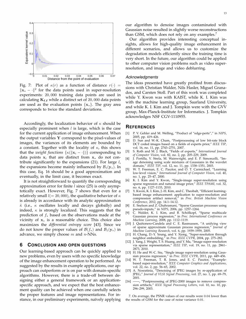
Distance from the point of evaluation

Equ

ival

ent k

erne

l val

ue

0 0.01 0.02 0.03 0.04 0.05 0.06 0.07−0.1

0

0.1

0.2

0.3

0.4

Fig. 7: Plot of κ(r) as a function of distance r(·) =‖x∗ − ·‖2 for the data points used in super-resolutionexperiments: 20, 000 training data points are used incalculating Kf ,f while a distinct set of 20, 000 data pointsare used as the evaluation points {x∗}. The gray areacorresponds to twice the standard deviations.

Accordingly, the localization behavior of κ should beespecially prominent when l is large, which is the casefor the current application of image enhancement. Whenthe output variables Y correspond to the pixel-values ofimages, the variances of its elements are bounded bya constant. Together with the locality of κ, this showsthat the weight functions {κ(‖xi − ·‖)} corresponding todata points xi that are distinct from x∗ do not con-tribute significantly to the expansions (21). For large l,the expansions become mainly influenced by B1(y∗). Inthis case, Eq. 16 should be a good approximation andeventually, in the limit case, it becomes exact.

It is not straightforward to quantify the correspondingapproximation error for finite l since (25) is only asymp-totically exact. However, Fig. 7 shows that even for arelatively small l(= 20, 000), the qualitative behavior of κis already in accordance with its analytic approximationκ (i.e., κ oscillates locally and decays globally) andindeed, κ is strongly localized. This suggests that theprediction of f∗ based on the observations made at thevicinity of x∗ is a reasonable choice. This choice alsomaximizes the differential entropy score [43]. Since wedo not know the proper values of B(f∗) and B1(y∗) inadvance, we simply choose m and n-NNs.

6 CONCLUSION AND OPEN QUESTIONS

Our learning-based approach can be quickly applied tonew problems, even by users with no specific knowledgeof the image enhancement operation to be performed. Assuggested by the results in example applications, our ap-proach can outperform or is on par with domain-specificalgorithms. However, there is a trade-off between de-signing either a general framework or an application-specific approach, and we expect that the best enhance-ment quality can be achieved when one carefully selectsthe proper features and image representations. For in-stance, in our preliminary experiments, naıvely applying

our algorithm to denoise images contaminated withGaussian noise resulted in slightly worse reconstructionsthan GSM, which does not rely on any examples.7

Our algorithm provides interesting conceptual in-sights, allows for high-quality image enhancement indifferent scenarios, and allows us to customize thedegradation models efficiently since the training time isvery short. In the future, our algorithm could be appliedto other computer vision problems such as video super-resolution, and image and video deblurring.

AcknowledgmentsThe ideas presented have greatly profited from discus-sions with Christian Walder, Nils Hasler, Miguel Grana-dos, and Carsten Stoll. Part of this work was completedwhile Y. Kwon was with KAIST, while K. I. Kim waswith the machine learning group, Saarland University,and while K. I. Kim and J. Tompkin were with the GVVgroup, Max-Planck-Institute for Informatics. J. Tompkinacknowledges NSF CGV-1110955.

REFERENCES[1] P. V. Gehler and M. Welling, “Product of “edge-perts”,” in NIPS,

2005, pp. 419–426.[2] D. Sun and W.-K. Cham, “Postprocessing of low bit-rate block

DCT coded images based on a fields of experts prior,” IEEE TIP,vol. 16, no. 11, pp. 2743–2751, 2007.

[3] S. Roth and M. J. Black, “Fields of experts,” International Journalof Computer Vision, vol. 82, no. 2, pp. 205–229, 2009.

[4] J. Portilla, V. Strela, M. Wainwright, and E. P. Simoncelli, “Im-age denoising using scale mixtures of Gaussians in the waveletdomain,” IEEE TIP, vol. 12, no. 11, pp. 1338–1351, 2003.

[5] W. T. Freeman, E. C. Pasztor, and O. T. Carmichael, “Learninglow-level vision,” International Journal of Computer Vision, vol. 40,no. 1, pp. 25–47, 2000.

[6] K. I. Kim and Y. Kwon, “Single-image super-resolution usingsparse regression and natural image prior,” IEEE TPAMI, vol. 32,no. 6, pp. 1127–1133, 2010.

[7] Y. Kwon, K. I. Kim, J.-H. Kim, and C. Theobalt, “Efficient learning-based image enhancement: application to super-resolution andcompression artifact removal,” in Proc. British Machine VisionConference, 2012, pp. 14.1–14.12.

[8] E. Snelson and Z. Ghahramani, “Sparse Gaussian processes usingpseudo-inputs,” in NIPS, 2006, pp. 1257–1264.

[9] C. Walder, K. I. Kim, and B. Scholkopf, “Sparse multiscaleGaussian process regression,” in Proc. International Conference onMachine Learning, 2008, pp. 1112–1119.

[10] J. Quinonero-Candela and C. E. Rasmussen, “A unifying viewof sparse approximate Gaussian process regression,” Journal ofMachine Learning Research, vol. 6, pp. 1939–1959, 2005.

[11] H. Chang, D.-Y. Yeung, and Y. Xiong, “Super-resolution throughneighbor embedding,” in Proc. IEEE CVPR, 2004, pp. 275–282.

[12] J. Yang, J. Wright, T. S. Huang, and Y. Ma, “Image super-resolutionvia sparse representation,” IEEE TIP, vol. 19, no. 11, pp. 2861–2873, 2010.

[13] H. He and W.-C. Siu, “Single image super-resolution using Gaus-sian process regression,” in Proc. IEEE CVPR, 2011, pp. 449–456.

[14] W. T. Freeman, T. R. Jones, and E. C. Pasztor, “Example-based super-resolution,” IEEE Computer Graphics and Applications,vol. 22, no. 2, pp. 56–65, 2002.

[15] A. Nosratinia, “Denoising of JPEG images by re-application ofJPEG,” Journal of VLSI Signal Processing, vol. 27, no. 1, pp. 69–79,2001.

[16] ——, “Postprocessing of JPEG-2000 images to remove compres-sion artifacts,” IEEE Signal Processing Letters, vol. 10, no. 10, pp.296–299, 2003.

7. On average, the PSNR values of our results were 0.04 lower thanthe results of GSM for the case of noise variance 0.01.

14

[17] A. Foi, V. Katkovnik, and K. Egiazarian, “Pointwise shape-adaptive DCT for high-quality denoising and deblocking ofgrayscale and color images,” IEEE TIP, vol. 16, no. 5, pp. 1395–1411, 2007.

[18] V. Laparra, J. Gutierrez, G. Camps-Valls, and J. Malo, “Imagedenoising with kernels based on natural image relations,” Journalof Machine Learning Research, vol. 11, pp. 873–903, 2010.

[19] G. Zhai, W. Lin, J. Cai, X. Yang, and W. Zhang, “Efficient quadtreebased block-shift filtering for deblocking and deringing,” Journalof Visual Communication and Image Representation, vol. 20, no. 8, pp.595–607, 2009.

[20] T. Wang and G. Zhai, “JPEG2000 image postprocessing with noveltrilateral deringing filter,” Optical Engineering, vol. 47, no. 2, pp.027 005–1–027 005–6, 2008.

[21] L. G. Gubin, B. T. Polyak, and E. V. Raik, “The method ofprojections for finding the common point of convex sets,” USSRComputational Mathematics and Mathematical Physics, vol. 7, no. 6,pp. 1–24, 1967.

[22] Y. Yang, N. P. Galatsanos, and A. K. Katsaggelos, “Projection-based spatially adaptive reconstruction of block-transform com-pressed images,” IEEE TIP, vol. 4, no. 7, pp. 896–908, 1995.

[23] X. Li, “Improved wavelet decoding via set theoretic estimation,”IEEE Trans. Circuits and Systems for Video Technology, vol. 15, no. 1,pp. 108–112, 2005.

[24] Z. Wang, A. C. Bovik, H. R. Sheikh, and E. P. Simoncelli, “Imagequality assessment: From error visibility to structural similarity,”IEEE TIP, vol. 13, no. 4, pp. 600–612, 2004.

[25] Z. Lin and H.-Y. Shum, “Fundamental limits of reconstruction-based superresolution algorithms under local translation,” IEEETPAMI, vol. 26, no. 1, pp. 83–97, 2004.

[26] S. Baker and T. Kanade, “Limits on super-resolution and how tobreak them,” IEEE TPAMI, vol. 24, no. 9, pp. 1167–1183, 2002.

[27] S. Chaudhuri, Super-Resolution Imaging. Springer, 2001.[28] M. F. Tappen, B. C. Russel, and W. T. Freeman, “Exploiting the

sparse derivative prior for super-resolution and image demosaic-ing,” in Proc. International Workshop on Statistical and ComputationalTheories of Vision, 2003.

[29] M. E. Tipping and C. M. Bishop, “Bayesian image super-resolution,” in NIPS, 2003, pp. 1303–1310.

[30] P. J. Liu, “Using Gaussian process regression to denoise imagesand remove artefacts from microarray data,” Ph.D. disserta-tion, Graduate Department of Computer Science, University ofToronto, Canada, 2007.

[31] D. Tschumperle and R. Deriche, “Vector-valued image regulariza-tion with PDEs: a common framework for different applications,”IEEE TPAMI, vol. 27, no. 4, pp. 506–517, 2005.

[32] G. Qiu, “MLP for adaptive postprocessing block-coded images,”IEEE Trans. Circuits and Systems for Video Technology, vol. 10, no. 8,pp. 1450–1454, 2000.

[33] K. Lee, D. S. Kim, and T. Kim, “Regression-based prediction forblocking artifact reduction in JPEG-compressed images,” IEEETIP, vol. 14, no. 1, pp. 36–49, 2005.

[34] H. A. Bourlard and N. Morgan, Connectionist Speech Recognition:A Hybrid Approach. Springer, 1993.

[35] L. C. Pickup, S. J. Roberts, and A. Zissermann, “A sampled textureprior for image super-resolution,” in NIPS, 2004, pp. 1587–1594.

[36] C. E. Rasmussen and C. K. I. Williams, Gaussian Processes forMachine Learning. MIT Press, 2006.

[37] M. Seeger, C. K. I. Williams, and N. Lawrence, “Fast forwardselection to speed up sparse Gaussian process regression,” in Proc.Artificial Intelligence and Statistics, 2003.

[38] E. Snelson and Z. Ghahramani, “Local and global sparse Gaussianprocess approximations,” in Proc. Artificial Intelligence and Statis-tics, 2007.

[39] G. C. Cawley, N. L. C. Talbot, and O. Chapelle, “Estimating pre-dictive variances with kernel ridge regression,” in Proc. MachineLearning Challenges: evaluating Predictive Uncertainty Visual ObjectClassification, and Recognizing Textual Entailment, 2006, pp. 56–77.

[40] C. M. Bishop, Pattern Recognition and Machine Learning. Springer,2006.

[41] B. W. Silverman, “Spline smoothing: the equivalent variable ker-nel method,” The Annals of Statistics, vol. 12, no. 3, pp. 898–916,1984.

[42] P. Sollich and C. K. I. Williams, “Using the equivalent kernelto understand Gaussian process regression,” in NIPS, 2005, pp.1313–1320.

[43] N. Lawrence, M. Seeger, and R. Herbrich, “Fast sparse Gaussianprocess methods: the informative vector machine,” in NIPS, 2003,pp. 625–632.

Younghee Kwon received BSc, MSc, and PhDdegrees in Computer Science at KAIST in 2000,2002, and 2009, respectively. Currently, he is asoftware engineer at Google. His research inter-est include computer vision, machine prediction,and parallel/distributed systems.

Kwang In Kim received a BSc in computer en-gineering from the Dongseo University in 1996,and MSc and PhD in computer engineering fromthe Kyungpook National University in 1998 and2000. He was a post-doctoral researcher atKAIST, at the Max-Planck-Institute for BiologicalCybernetics, at Saarland University, and at theMax-Planck-Institute for Informatics, from 2000to 2013. Currently, he is a lecturer at the Schoolof Computing and Communications, LancasterUniversity. His research interests include ma-

chine learning, computer vision and computer graphics.

James Tompkin received an MSci degree inComputer Science from King’s College Londonin 2006, and an EngD degree in Virtual Envi-ronments, Imaging, and Visualization from Uni-versity College London in 2012. He was a post-doctoral researcher at the Max-Planck-Institutefor Informatics from 2012 to 2014, and is cur-rently a post-doctoral researcher at Harvard Uni-versity. His research applies vision, graphics,machine learning, and interaction to create newvisual computing tools and experiences.

Jin Hyung Kim is director of the Software Pol-icy & Research Institute in Seoul, Korea. Heworked at Hughes Research Laboratories afterobtaining his PhD degree in Computer Scienceat University of California Los Angeles, USA, in1983. He has served as professor and depart-ment chair in the computer science departmentat KAIST, as President of Korean R&D Informa-tion Center, as President of Korean InformationScience Society, as a member of the NationalAcademy of Engineering of Korea, and as fel-

lows of the Korean Academy of Science and Technology and of theInternational Association of Pattern Recognition. He received the Orderof Service Merit Green Stripes from the Korean Government in 2001.

Christian Theobalt is a Professor of ComputerScience at the Max-Planck-Institute for Infor-matics and Saarland University in Saarbrucken,Germany. He researches problems that lie onthe boundary between the fields of ComputerVision and Computer Graphics, such as dynamic3D scene reconstruction and marker-less motioncapture. He received the Otto Hahn Medal of theMax-Planck Society in 2007, the EUROGRAPH-ICS Young Researcher Award in 2009, and theGerman Pattern Recognition Award in 2012.