The Visual Computer manuscript No.(will be inserted by the editor)

Takahiro Harada · Seiichi Koshizuka · Yoichiro Kawaguchi

Smoothed Particle Hydrodynamics on GPUs

Abstract In this paper, we present a Smoothed Parti-cle Hydrodynamics (SPH) implementation algorithm onGPUs. To compute a force on a particle, neighboring par-ticles have to be searched. However, implementation of aneighboring particle search on GPUs is not straightfor-ward. We developed a method that can search for neigh-boring particles on GPUs, which enabled us to imple-ment the SPH simulation entirely on GPUs. Since all ofthe computation is done on GPUs and no CPU process-ing is needed, the proposed algorithm can exploit themassive computational power of GPUs. Consequently,the simulation speed is many times increased with theproposed method.

Keywords Fluid simulation · Particle method ·Smoothed Particle Hydrodynamics · Graphics hardware ·General Purpose Computation on GPUs

1 Introduction

At the present time, physically based simulation is widelyused in computer graphics to produce animations. Eventhe complex motion of fluid can be generated by simu-lation. There is a need for faster simulation in real-timeapplications, such as computer games, virtual surgeryand so on. However, the computational burden of fluidsimulation is high, especially when we simulate free sur-face flow, and so it is difficult to apply fluid simulation toreal-time applications. Thus real-time simulation of freesurface flow is an open research area.

In this paper, we accelerated Smoothed Particle Hy-drodynamics (SPH), which is a simulation method offree surface flow, by using of Graphics Processing Units(GPUs). No study has so far accomplished acceleration

T.Harada7-3-1, Hongo, Bunkyo-ku, Tokyo, JapanTel.: +81-3-5841-5936E-mail: takahiroharada@iii.u-tokyo.ac.jp

S. Koshizuka and Y.Kawaguchi7-3-1, Hongo, Bunkyo-ku, Tokyo, Japan

of particle-based fluid simulation by implementing theentire algorithm on GPUs. This is because a neighboringparticle search cannot be easily implemented on GPUs.We developed a method that can search for neighboringparticles on GPUs by introducing a three-dimensionalgrid. The proposed method can exploit the computa-tional power of GPUs because all of the computationis done on the GPU. As a result, SPH simulation is ac-celerated drastically and tens of thousands of particlesare simulated in real-time.

2 Related Works

Foster et al. introduced the three-dimensional Navie-Stokesequation to the computer graphics community[8] andStam et al. also introduced the semi-Lagrangian method[34].For free surface flow, Foster et al. used the level setmethod to track the interface[7]. Enright et al. devel-oped the particle-level set method by coupling the levelset method with lagrangian particles[6]. Bargteil et al.presented another surface tracking method that used ex-plicit and implicit surface representation[2]. Coupling offluid and rigid bodies[3], viscoelastic fluid[9], interactionwith thin shells[10], surface tension, vortex particles, cou-pling of two and three-dimensional computation[14], oc-tree grids[25] and tetrahedron meshes[17] have been stud-ied.

These studies used grids, but there are other meth-ods that can solve the motion of a fluid. These are calledparticle methods. Moving Particle Semi-implicit (MPS)method[20] and Smoothed Particle Hydrodynamics (SPH)[27] are particle methods that can compute fluid motion.Premoze et al. introduced the MPS method, which real-ized incompressibility by solving the Poisson equation onparticles and has been well studied in areas such as com-putational mechanics, to the graphics community[32].Muller et al. applied SPH, which had been developedin astronomy, for fluid simulation[28]. They showed thatSPH could be applied for interactive applications andused a few thousand of particles. However, the number

2 Takahiro Harada et al.

was not enough to obtain sufficient results. Viscoelasticfluids[4], coupling with deformable bodies[29] and multi-phase flow[30] were also studied. Kipfer et al. acceleratedSPH using a data structure suitable for sparse particlesystems[16].

The growth of the computational power of GPUs,which are designed for three-dimensional graphics tasks,has been tremendous. Thus there are a lot of studiesthat use GPUs to accelerate non-graphic tasks, such ascellular automata simulation[13], particle simulation[15][19], solving linear equations[21] and so on. We can findan overview of these studies in a review paper[31]. Also,there were studies on the acceleration of fluid simulation,i.e., simplefied fluid simulation and crowd simulation[5],two-dimensional fluid simulation[11], three-dimensionalfluid simulation[23], cloud simulation[12] and Lattice Boltz-mann Method simulation[22]. Amada et al. used the GPUfor the acceleration of SPH. However, they could notexploit the power of the GPU because the neighboringparticle search was done on CPUs and the data weretransferred to GPUs at each time step[1]. Kolb et al.also implemented SPH on the GPU[18]. Although theirmethod could implement SPH entirely on the GPU, theysuffered from interpolation error because physical valueson the grid were computed and those at particles wereinterpolated. A technique for neighboring particle searchon GPUs is also found in [33]. They developed a methodto generate a data structure for finding nearest neigh-bors called stencil routing. A complicated texture foot-print have to be prepared in advance and it needs a largetexture when it applied to a large computation domainbecause a spatial grid is represented by a few texels.

There have been few studies on the acceleration offree surface flow simulation using GPUs.

3 Smoothed Particle Hydrodynacimcs

3.1 Governing Equations

The governing equations for incompressible flow are themass conservation equation and the momentum conser-vation equation

Dρ

Dt= 0 (1)

DUDt

= −1ρ∇P + ν∇2U + g (2)

where ρ,U, P, ν,g are density, velocity, pressure, dynamicviscosity coefficient of the fluid and gravitational accel-eration, respectively.

3.2 Discretization

In SPH, a physical value at position x is calculated as aweighted sum of physical values φj of neighboring parti-cles j

φ(x) =∑

j

mjφj

ρjW (x − xj) (3)

where mj , ρj ,xj are the mass, density and position ofparticle j, respectively and W is a weight function.

The density of fluid is calculated with eqn.3 as

ρ(x) =∑

j

mjW (x − xj). (4)

The pressure of fluid is calculated via the constitutiveequation

p = p0 + k(ρ − ρ0) (5)

where p0, ρ0 are the rest pressure and density, respec-tively.

To compute the momentum conservation equation,gradient and laplacian operators, which are used to solvethe pressure and viscosity forces on particles, have tobe modeled. The pressure force Fpress and the viscosityforce Fvis are computed as

Fpressi = −

∑j

mjpi + pj

2ρj∇Wpress(rij) (6)

Fvisi = ν

∑j

mjvj − vi

ρj∇Wvis(rij) (7)

where rij is the relative position vector and is calculatedas rij = rj − ri where ri, rj are the positions of particlesi and j, respectively.

The weight functions used by Muller et al. are alsoused in this study[28]. The weight functions for the pres-sure, viscosity and other terms are designed as follows.

∇Wpress(r) =45πr6

e

(re − |r|)3 r|r|

(8)

∇Wvis(r) =45πr6

e

(re − |r|) (9)

W (r) =315

64πr9e

(r2e − |r|2)3 (10)

This value is 0 outside of the effective radius re in thesefunctions.

3.3 Boundary Condition

3.3.1 Pressure term

Because the pressure force leads to the constant densityof fluid when we solve incompressible flow, it retains thedistance d between particles, which is the rest distance.We assume that particle i is at the distance |riw| to the

Smoothed Particle Hydrodynamics on GPUs 3

riw

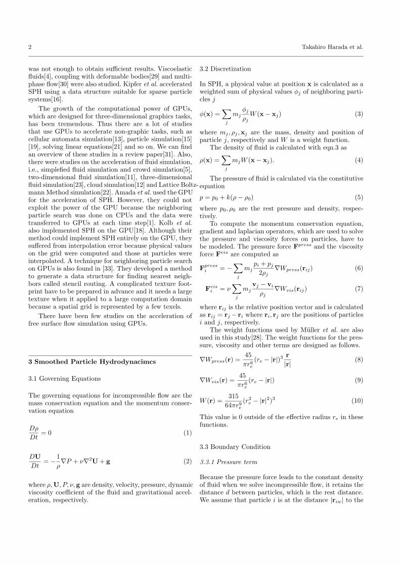
Fig. 1 Distribution of wall particles.

wall boundary and |riw| < d. The pressure force pushesparticle i back to the distance d in the direction of n(ri)which is the normal vector of the wall boundary. Thus,the pressure force Fpress

i is modeled as

Fpressi = mi

∆xi

dt2

= mi(d − |riw|)n(ri)

dt2. (11)

3.3.2 Density

When a particle is within the effective radius re to thewall boundary, the contribution of the wall boundaryto the density has to be estimated. If wall particles aregenerated within the wall boundary, their contributionas well as those of fluid particles can be calculated.

ρi(ri) =∑

j∈fluid

mjW (rij) +∑

j∈wall

mjW (rij) (12)

The distribution of wall particles is determined uniquelyby assuming that they are distributed perpendicular tothe vertical line to the wall boundary and the mean cur-vature of the boundary is 0 as shown in fig.1. Therefore,the contribution of the wall boundary is a function of thedistance |riw| to the wall boundary.

ρi(ri) =∑

j∈fluid

mjW (rij) + Zrhowall(|riw|) (13)

We call Zrhowall as wall weight function. Since this wall

weigh function depends on the distance |riw|, it can beprecomputed and referred in the fluid simulation. Pre-computation of the wall weight function can be done byplacing wall particles and adding their weighted values.This function is computed in advance at a few pointswithin the effective radius re and the function at an ar-bitrary position is calculated by linear interpolation ofthem.

To obtain the distance to the wall boundary, we haveto compute the distance from each particle to all the

Position(1)Density(1)

Bucket

Generation

Velocity

Update

Density

Computation

Position

Update

Velocity(1)

BucketDistance

Function

WallWeight

Function

Density(2)

Velocity(2)

Position(2)

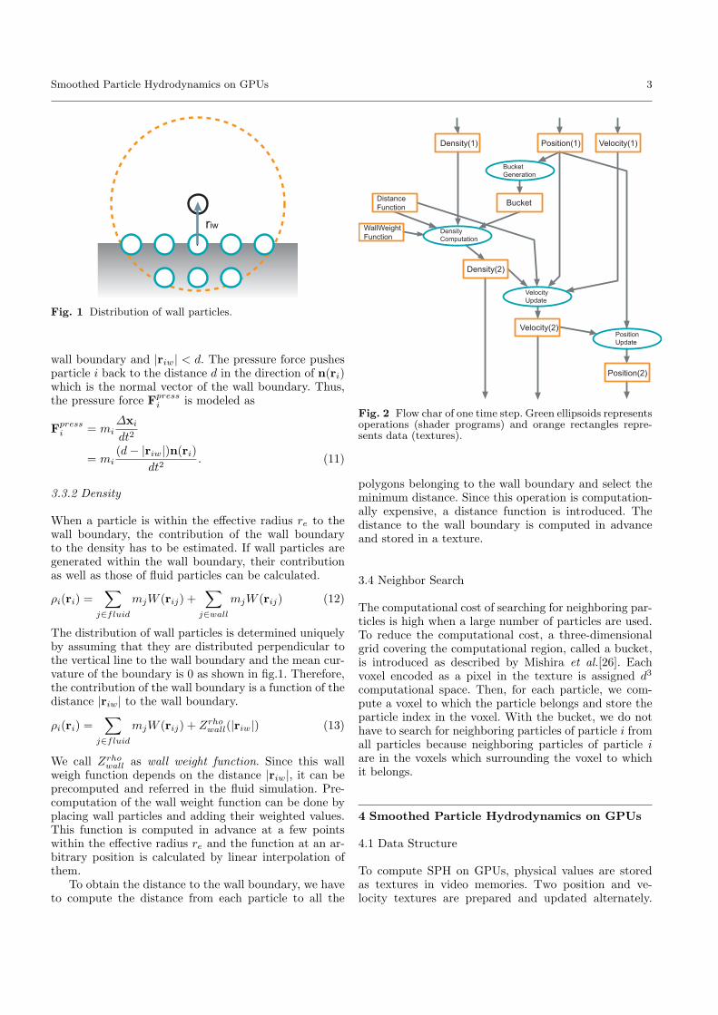
Fig. 2 Flow char of one time step. Green ellipsoids representsoperations (shader programs) and orange rectangles repre-sents data (textures).

polygons belonging to the wall boundary and select theminimum distance. Since this operation is computation-ally expensive, a distance function is introduced. Thedistance to the wall boundary is computed in advanceand stored in a texture.

3.4 Neighbor Search

The computational cost of searching for neighboring par-ticles is high when a large number of particles are used.To reduce the computational cost, a three-dimensionalgrid covering the computational region, called a bucket,is introduced as described by Mishira et al.[26]. Eachvoxel encoded as a pixel in the texture is assigned d3

computational space. Then, for each particle, we com-pute a voxel to which the particle belongs and store theparticle index in the voxel. With the bucket, we do nothave to search for neighboring particles of particle i fromall particles because neighboring particles of particle iare in the voxels which surrounding the voxel to whichit belongs.

4 Smoothed Particle Hydrodynamics on GPUs

4.1 Data Structure

To compute SPH on GPUs, physical values are storedas textures in video memories. Two position and ve-locity textures are prepared and updated alternately.

4 Takahiro Harada et al.

A bucket texture and a density texture are also pre-pared. Although a bucket is a three-dimensional array,current GPUs cannot write to a three-dimensional bufferdirectly. Therefore, we employed a flat 3D texture inwhich a three-dimensional array is divided into a set oftwo-dimensional arrays and is then placed in a large tex-ture. The detailed description can be found in [12]. Aswell as these values updated in every iteration, staticvalues are stored in textures. The wall weight functionis stored in a one-dimensional texture and a distancefunction which is a three-dimensional array is stored ina three-dimensional texture. The reason why a flat 3Dtexture is not employed is that the distance function isnot updated during a simulation.

4.2 Algorithm Overview

One time step of SPH is performed in four steps.

1. Bucket Generation2. Density Computation3. Velocity Update4. Position Update

The implementation detail is described in the followingsubsections. The flowchart is shown in Figure 2.

4.3 Bucket Generation

Since the number of particle indices stored in a voxel isnot always one, a bucket cannot be generated correctlyby parallel processing of all particle indices. This is be-cause we have to count the number of particle indicesstored in a voxel if there are multiple particle indices inthe voxel.

Assume that the maximum particle number stored ina voxel is one. The bucket is correctly generated by ren-dering vertices which are made correspondence to eachparticles at the corresponding particle center position.The particle indices are set to the color of the vertices.This operation can be performed using vertex texturefetch. However, the operation cannot generate a bucketcorrectly in the case where there is more than one par-ticle index in a voxel.

The proposed method can generate a bucket that canstore less than four particle indices in a voxel. We assumethat particle indices i0, i1, i2, i3 are stored in a voxel andthey are arranged as i0 < i1 < i2 < i3. The verticescorresponding to these particles are drawn and processedin ascending order of the indices[15]. We are going tostore the indices i0, i1, i2, i3 in the red, green, blue andalpha (RGBA) channels in a pixel, respectively by fourrendering passes. In each pass, the particle indices arestored in ascending order. Color mask, depth buffer andstencil buffer are used to generate a bucket correctly.

Distance Function

x,y,z

d

Wall Weight Function

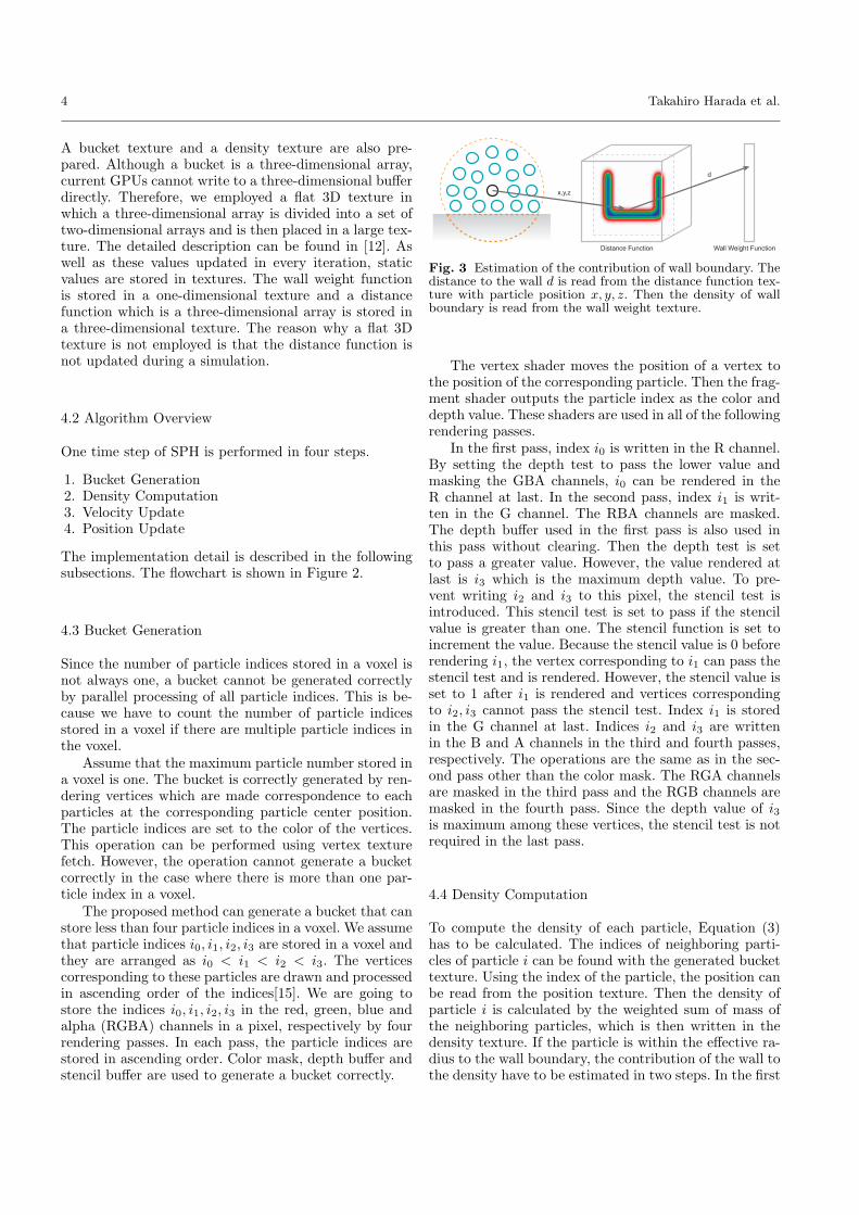
Fig. 3 Estimation of the contribution of wall boundary. Thedistance to the wall d is read from the distance function tex-ture with particle position x, y, z. Then the density of wallboundary is read from the wall weight texture.

The vertex shader moves the position of a vertex tothe position of the corresponding particle. Then the frag-ment shader outputs the particle index as the color anddepth value. These shaders are used in all of the followingrendering passes.

In the first pass, index i0 is written in the R channel.By setting the depth test to pass the lower value andmasking the GBA channels, i0 can be rendered in theR channel at last. In the second pass, index i1 is writ-ten in the G channel. The RBA channels are masked.The depth buffer used in the first pass is also used inthis pass without clearing. Then the depth test is setto pass a greater value. However, the value rendered atlast is i3 which is the maximum depth value. To pre-vent writing i2 and i3 to this pixel, the stencil test isintroduced. This stencil test is set to pass if the stencilvalue is greater than one. The stencil function is set toincrement the value. Because the stencil value is 0 beforerendering i1, the vertex corresponding to i1 can pass thestencil test and is rendered. However, the stencil value isset to 1 after i1 is rendered and vertices correspondingto i2, i3 cannot pass the stencil test. Index i1 is storedin the G channel at last. Indices i2 and i3 are writtenin the B and A channels in the third and fourth passes,respectively. The operations are the same as in the sec-ond pass other than the color mask. The RGA channelsare masked in the third pass and the RGB channels aremasked in the fourth pass. Since the depth value of i3is maximum among these vertices, the stencil test is notrequired in the last pass.

4.4 Density Computation

To compute the density of each particle, Equation (3)has to be calculated. The indices of neighboring parti-cles of particle i can be found with the generated buckettexture. Using the index of the particle, the position canbe read from the position texture. Then the density ofparticle i is calculated by the weighted sum of mass ofthe neighboring particles, which is then written in thedensity texture. If the particle is within the effective ra-dius to the wall boundary, the contribution of the wall tothe density have to be estimated in two steps. In the first

Smoothed Particle Hydrodynamics on GPUs 5

step, the distance from particle i to the wall is looked upfrom the distance function stored in a three-dimensionaltexture. Then the wall weight function stored in a one-dimensional texture is read with a texture coordinate cal-culated by the distance to the wall. This procedure is il-lustrated in Figure 3. The contribution of wall boundaryto the density is added to the density calculated amongparticles.

4.5 Velocity Update

To compute the pressure and viscosity forces, neighbor-ing particles have to be searched for again. The proce-dure is the same as that for the density computation.These forces are computed using Equations (6) and (7).The pressure force from the wall boundary is computedusing the distance function. Then, the updated velocityis written in another velocity texture.

4.6 Position Update

Using the updated velocity texture, the position is cal-culated with an explicit Euler integration.

x′i = xi + vidt (14)

where xi and vi are the previous position and veloc-ity of particle i, respectively. The updated position x′

i iswritten to another position texture. Although there arehigher order schemes, they were not introduced becausewe did not encounter any stability problems.

5 Results and Discussion

The proposed method was implemented on a PC with aCore 2 X6800 2.93GHz CPU, 2.0GB RAM and a GeForce8800GTX GPU. The programs were written in C++ andOpenGL and the shader programs were written in C forGraphics.

In Figures 4 and 5 we show real-time simulation re-sults. Approximately 60,000 particles were used in bothsimulations and they ran at about 17 frames per second.Previous studies used several thousand particles for real-time simulation, However, the proposed method enabledus to use 10 times as many particles as before in real-time simulation. The simulation results were renderedby using pointsprite and vertex texture fetch. The colorof particles indicates the particle number density. Par-ticles with high density are rendered in blue color andthose with low density are rendered in white. The pro-posed method can accelerate offline simulation as well asreal-time simulations. In Figures 6, 7 and 8, the simu-lated particle positions are read back to the CPU andrendered with a raytracer after the simulations. Surfacesof fluid is extracted from particles by using Marching

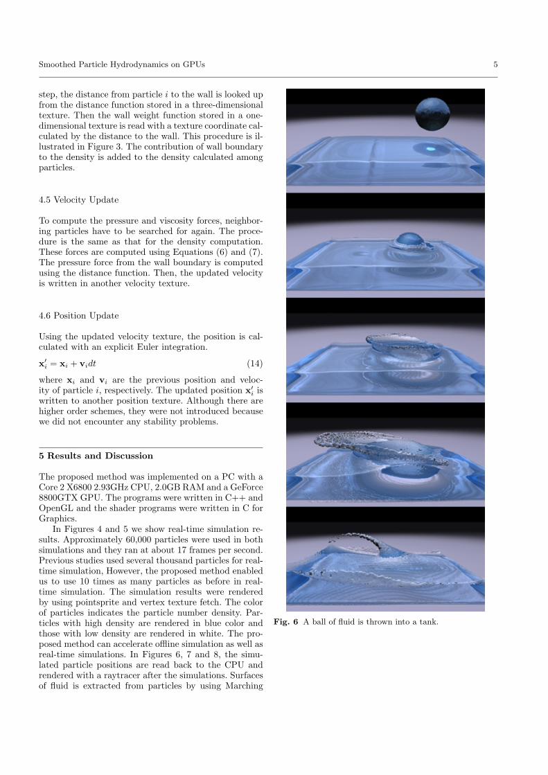
Fig. 6 A ball of fluid is thrown into a tank.

6 Takahiro Harada et al.

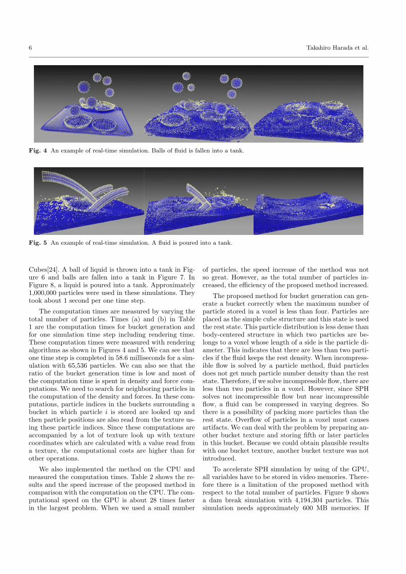
Fig. 4 An example of real-time simulation. Balls of fluid is fallen into a tank.

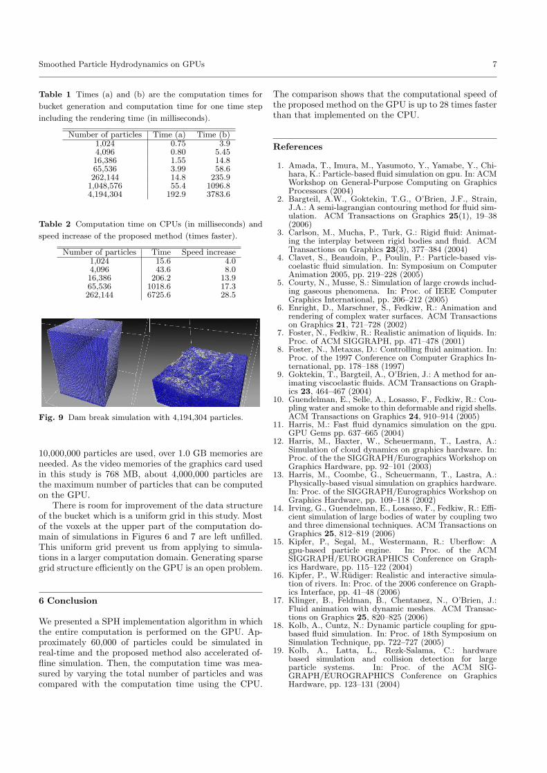
Fig. 5 An example of real-time simulation. A fluid is poured into a tank.

Cubes[24]. A ball of liquid is thrown into a tank in Fig-ure 6 and balls are fallen into a tank in Figure 7. InFigure 8, a liquid is poured into a tank. Approximately1,000,000 particles were used in these simulations. Theytook about 1 second per one time step.

The computation times are measured by varying thetotal number of particles. Times (a) and (b) in Table1 are the computation times for bucket generation andfor one simulation time step including rendering time.These computation times were measured with renderingalgorithms as shown in Figures 4 and 5. We can see thatone time step is completed in 58.6 milliseconds for a sim-ulation with 65,536 particles. We can also see that theratio of the bucket generation time is low and most ofthe computation time is spent in density and force com-putations. We need to search for neighboring particles inthe computation of the density and forces. In these com-putations, particle indices in the buckets surrounding abucket in which particle i is stored are looked up andthen particle positions are also read from the texture us-ing these particle indices. Since these computations areaccompanied by a lot of texture look up with texturecoordinates which are calculated with a value read froma texture, the computational costs are higher than forother operations.

We also implemented the method on the CPU andmeasured the computation times. Table 2 shows the re-sults and the speed increase of the proposed method incomparison with the computation on the CPU. The com-putational speed on the GPU is about 28 times fasterin the largest problem. When we used a small number

of particles, the speed increase of the method was notso great. However, as the total number of particles in-creased, the efficiency of the proposed method increased.

The proposed method for bucket generation can gen-erate a bucket correctly when the maximum number ofparticle stored in a voxel is less than four. Particles areplaced as the simple cube structure and this state is usedthe rest state. This particle distribution is less dense thanbody-centered structure in which two particles are be-longs to a voxel whose length of a side is the particle di-ameter. This indicates that there are less than two parti-cles if the fluid keeps the rest density. When incompress-ible flow is solved by a particle method, fluid particlesdoes not get much particle number density than the reststate. Therefore, if we solve incompressible flow, there areless than two particles in a voxel. However, since SPHsolves not incompressible flow but near incompressibleflow, a fluid can be compressed in varying degrees. Sothere is a possibility of packing more particles than therest state. Overflow of particles in a voxel must causesartifacts. We can deal with the problem by preparing an-other bucket texture and storing fifth or later particlesin this bucket. Because we could obtain plausible resultswith one bucket texture, another bucket texture was notintroduced.

To accelerate SPH simulation by using of the GPU,all variables have to be stored in video memories. There-fore there is a limitation of the proposed method withrespect to the total number of particles. Figure 9 showsa dam break simulation with 4,194,304 particles. Thissimulation needs approximately 600 MB memories. If

Smoothed Particle Hydrodynamics on GPUs 7

Table 1 Times (a) and (b) are the computation times for

bucket generation and computation time for one time step

including the rendering time (in milliseconds).

Number of particles Time (a) Time (b)1,024 0.75 3.94,096 0.80 5.4516,386 1.55 14.865,536 3.99 58.6262,144 14.8 235.9

1,048,576 55.4 1096.84,194,304 192.9 3783.6

Table 2 Computation time on CPUs (in milliseconds) and

speed increase of the proposed method (times faster).

Number of particles Time Speed increase1,024 15.6 4.04,096 43.6 8.016,386 206.2 13.965,536 1018.6 17.3262,144 6725.6 28.5

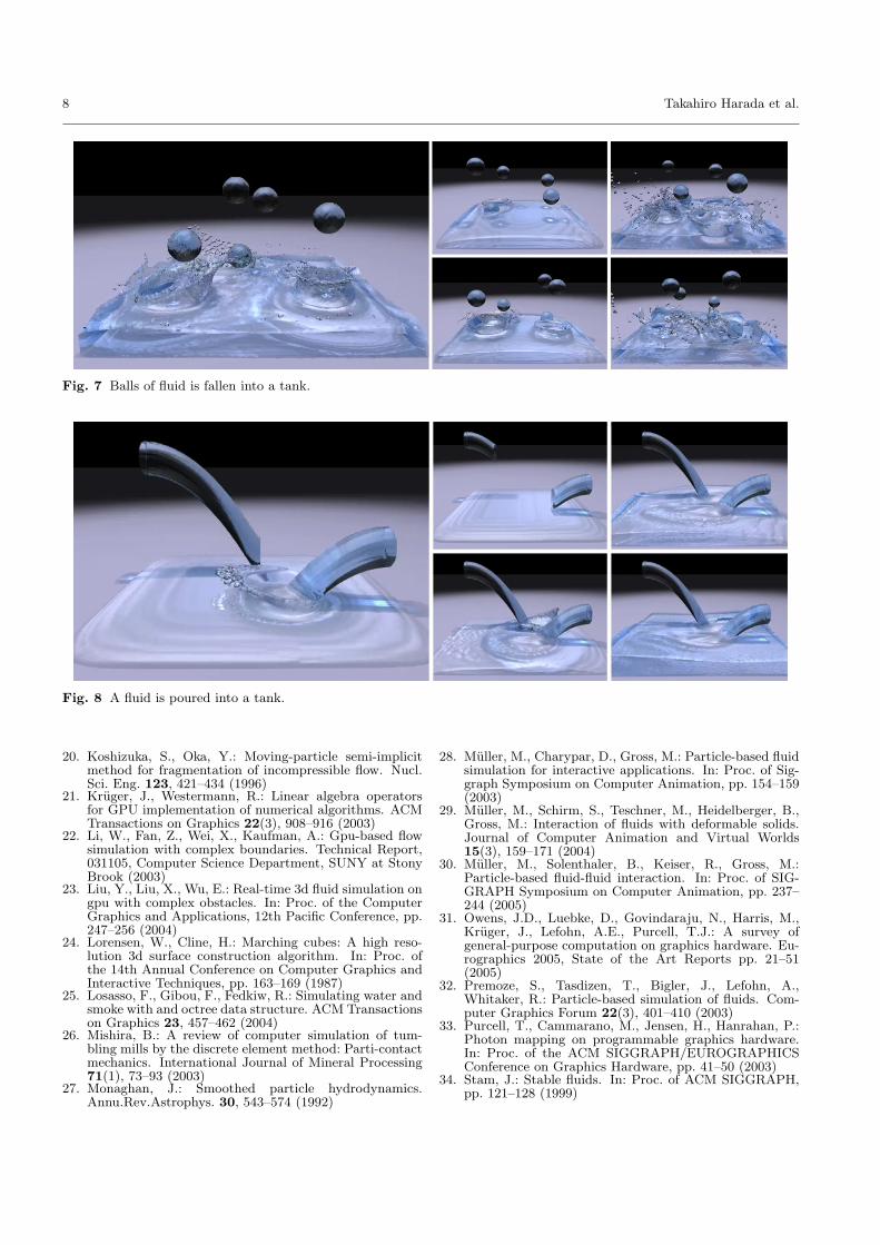
Fig. 9 Dam break simulation with 4,194,304 particles.

10,000,000 particles are used, over 1.0 GB memories areneeded. As the video memories of the graphics card usedin this study is 768 MB, about 4,000,000 particles arethe maximum number of particles that can be computedon the GPU.

There is room for improvement of the data structureof the bucket which is a uniform grid in this study. Mostof the voxels at the upper part of the computation do-main of simulations in Figures 6 and 7 are left unfilled.This uniform grid prevent us from applying to simula-tions in a larger computation domain. Generating sparsegrid structure efficiently on the GPU is an open problem.

6 Conclusion

We presented a SPH implementation algorithm in whichthe entire computation is performed on the GPU. Ap-proximately 60,000 of particles could be simulated inreal-time and the proposed method also accelerated of-fline simulation. Then, the computation time was mea-sured by varying the total number of particles and wascompared with the computation time using the CPU.

The comparison shows that the computational speed ofthe proposed method on the GPU is up to 28 times fasterthan that implemented on the CPU.

References

1. Amada, T., Imura, M., Yasumoto, Y., Yamabe, Y., Chi-hara, K.: Particle-based fluid simulation on gpu. In: ACMWorkshop on General-Purpose Computing on GraphicsProcessors (2004)

2. Bargteil, A.W., Goktekin, T.G., O’Brien, J.F., Strain,J.A.: A semi-lagrangian contouring method for fluid sim-ulation. ACM Transactions on Graphics 25(1), 19–38(2006)

3. Carlson, M., Mucha, P., Turk, G.: Rigid fluid: Animat-ing the interplay between rigid bodies and fluid. ACMTransactions on Graphics 23(3), 377–384 (2004)

4. Clavet, S., Beaudoin, P., Poulin, P.: Particle-based vis-coelastic fluid simulation. In: Symposium on ComputerAnimation 2005, pp. 219–228 (2005)

5. Courty, N., Musse, S.: Simulation of large crowds includ-ing gaseous phenomena. In: Proc. of IEEE ComputerGraphics International, pp. 206–212 (2005)

6. Enright, D., Marschner, S., Fedkiw, R.: Animation andrendering of complex water surfaces. ACM Transactionson Graphics 21, 721–728 (2002)

7. Foster, N., Fedkiw, R.: Realistic animation of liquids. In:Proc. of ACM SIGGRAPH, pp. 471–478 (2001)

8. Foster, N., Metaxas, D.: Controlling fluid animation. In:Proc. of the 1997 Conference on Computer Graphics In-ternational, pp. 178–188 (1997)

9. Goktekin, T., Bargteil, A., O’Brien, J.: A method for an-imating viscoelastic fluids. ACM Transactions on Graph-ics 23, 464–467 (2004)

10. Guendelman, E., Selle, A., Losasso, F., Fedkiw, R.: Cou-pling water and smoke to thin deformable and rigid shells.ACM Transactions on Graphics 24, 910–914 (2005)

11. Harris, M.: Fast fluid dynamics simulation on the gpu.GPU Gems pp. 637–665 (2004)

12. Harris, M., Baxter, W., Scheuermann, T., Lastra, A.:Simulation of cloud dynamics on graphics hardware. In:Proc. of the the SIGGRAPH/Eurographics Workshop onGraphics Hardware, pp. 92–101 (2003)

13. Harris, M., Coombe, G., Scheuermann, T., Lastra, A.:Physically-based visual simulation on graphics hardware.In: Proc. of the SIGGRAPH/Eurographics Workshop onGraphics Hardware, pp. 109–118 (2002)

14. Irving, G., Guendelman, E., Losasso, F., Fedkiw, R.: Effi-cient simulation of large bodies of water by coupling twoand three dimensional techniques. ACM Transactions onGraphics 25, 812–819 (2006)

15. Kipfer, P., Segal, M., Westermann, R.: Uberflow: Agpu-based particle engine. In: Proc. of the ACMSIGGRAPH/EUROGRAPHICS Conference on Graph-ics Hardware, pp. 115–122 (2004)

16. Kipfer, P., W.Rudiger: Realistic and interactive simula-tion of rivers. In: Proc. of the 2006 conference on Graph-ics Interface, pp. 41–48 (2006)

17. Klinger, B., Feldman, B., Chentanez, N., O’Brien, J.:Fluid animation with dynamic meshes. ACM Transac-tions on Graphics 25, 820–825 (2006)

18. Kolb, A., Cuntz, N.: Dynamic particle coupling for gpu-based fluid simulation. In: Proc. of 18th Symposium onSimulation Technique, pp. 722–727 (2005)

19. Kolb, A., Latta, L., Rezk-Salama, C.: hardwarebased simulation and collision detection for largeparticle systems. In: Proc. of the ACM SIG-GRAPH/EUROGRAPHICS Conference on GraphicsHardware, pp. 123–131 (2004)

8 Takahiro Harada et al.

Fig. 7 Balls of fluid is fallen into a tank.

Fig. 8 A fluid is poured into a tank.

20. Koshizuka, S., Oka, Y.: Moving-particle semi-implicitmethod for fragmentation of incompressible flow. Nucl.Sci. Eng. 123, 421–434 (1996)

21. Kruger, J., Westermann, R.: Linear algebra operatorsfor GPU implementation of numerical algorithms. ACMTransactions on Graphics 22(3), 908–916 (2003)

22. Li, W., Fan, Z., Wei, X., Kaufman, A.: Gpu-based flowsimulation with complex boundaries. Technical Report,031105, Computer Science Department, SUNY at StonyBrook (2003)

23. Liu, Y., Liu, X., Wu, E.: Real-time 3d fluid simulation ongpu with complex obstacles. In: Proc. of the ComputerGraphics and Applications, 12th Pacific Conference, pp.247–256 (2004)

24. Lorensen, W., Cline, H.: Marching cubes: A high reso-lution 3d surface construction algorithm. In: Proc. ofthe 14th Annual Conference on Computer Graphics andInteractive Techniques, pp. 163–169 (1987)

25. Losasso, F., Gibou, F., Fedkiw, R.: Simulating water andsmoke with and octree data structure. ACM Transactionson Graphics 23, 457–462 (2004)

26. Mishira, B.: A review of computer simulation of tum-bling mills by the discrete element method: Parti-contactmechanics. International Journal of Mineral Processing71(1), 73–93 (2003)

27. Monaghan, J.: Smoothed particle hydrodynamics.Annu.Rev.Astrophys. 30, 543–574 (1992)

28. Muller, M., Charypar, D., Gross, M.: Particle-based fluidsimulation for interactive applications. In: Proc. of Sig-graph Symposium on Computer Animation, pp. 154–159(2003)

29. Muller, M., Schirm, S., Teschner, M., Heidelberger, B.,Gross, M.: Interaction of fluids with deformable solids.Journal of Computer Animation and Virtual Worlds15(3), 159–171 (2004)

30. Muller, M., Solenthaler, B., Keiser, R., Gross, M.:Particle-based fluid-fluid interaction. In: Proc. of SIG-GRAPH Symposium on Computer Animation, pp. 237–244 (2005)

31. Owens, J.D., Luebke, D., Govindaraju, N., Harris, M.,Kruger, J., Lefohn, A.E., Purcell, T.J.: A survey ofgeneral-purpose computation on graphics hardware. Eu-rographics 2005, State of the Art Reports pp. 21–51(2005)

32. Premoze, S., Tasdizen, T., Bigler, J., Lefohn, A.,Whitaker, R.: Particle-based simulation of fluids. Com-puter Graphics Forum 22(3), 401–410 (2003)

33. Purcell, T., Cammarano, M., Jensen, H., Hanrahan, P.:Photon mapping on programmable graphics hardware.In: Proc. of the ACM SIGGRAPH/EUROGRAPHICSConference on Graphics Hardware, pp. 41–50 (2003)

34. Stam, J.: Stable fluids. In: Proc. of ACM SIGGRAPH,pp. 121–128 (1999)