Yin-Yang grid in Numerical Relativity

Wasilij Barsukow1,2

Pedro Montero1, Ewald Muller1, Thomas W. Baumgarte3

1Max-Planck-Institute for Astrophysics Garching2University of Heidelberg, 3Bowdoin College

June 30, 2014

1 / 273

Outline

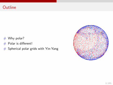
# Why polar?

# Polar is different!

# Spherical polar grids with Yin-Yang

2 / 273

Introduction

Astrophysical applications

# Astrophysical objects often have roughly spherical shapes with a largevariety of different length scales

# In certain situations a cartesian grid induces artefacts that spoil theresults of the simulation

3 / 273

Introduction

Relativity

Gµν = 8πTµν

4 / 273

Introduction

RelativityBaumgarte et al. (2012)

γij := e−4φγij conformal metric

Aij := e−4φ(Kij −

1

3γijK

)conformally rescaled traceless extr. curv.

Γijk background connection (spherical polar!)

∆Γijk := Γijk − Γijk , Λi := γjk∆Γijk

∂⊥ := ∂t − Lβ

% := nanbTab

Si := −γianbTab

Sij := γiaγjbTab

S := γijSij

with na = (−α, 0, 0, 0)

∂⊥γij = −2

3γij Dkβ

k − 2αAij

∂⊥Aij = −2

3Aij Dkβ

k − 2αAik Akj + αAijK + e4φ

[−2αDi Djφ + 4αDiφDjφ + 4D(iαDj)φ− Di Djα + α(Rij − 8πSij )

]TF

∂⊥φ =1

6Dkβ

k −1

6αK

∂⊥K =α

3K2 + αAij A

ij − e−4φ(D2α + 2D i

αDiφ) + 4πα(% + S)

∂⊥Λi = γjk Dj Dkβ

i +2

3Λi Djβ

j +1

3D i Djβ

j − 2Ajk (δi j∂kα− 6αδi j∂kφ− α∆Γijk )−4

3αγ

ij∂jK − 16παγ ijSj

Rij = −1

2γkl Dk D`γij + γk(i Dj)Λk + Λk∆Γ(ij)k + γ

k`(2∆Γmk(i∆Γj)m` + ∆Γmik∆Γmjl )

∂tα = −2αK

∂tβi = B i

∂tBi =

3

4∂t Λi

5 / 273

Introduction

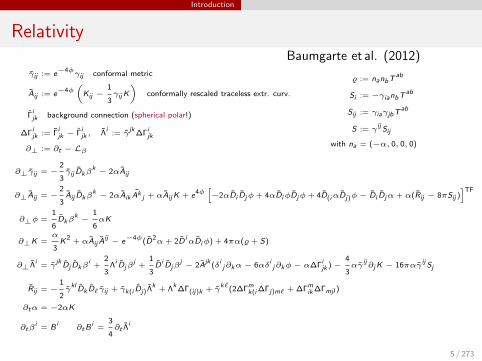
RelativityBaumgarte et al. (2012)

γij := e−4φγij conformal metric

Aij := e−4φ(Kij −

1

3γijK

)conformally rescaled traceless extr. curv.

Γijk background connection (spherical polar!)

∆Γijk := Γijk − Γijk , Λi := γjk∆Γijk

∂⊥ := ∂t − Lβ

% := nanbTab

Si := −γianbTab

Sij := γiaγjbTab

S := γijSij

with na = (−α, 0, 0, 0)

∂⊥γij = −2

3γij Dkβ

k − 2αAij

∂⊥Aij = −2

3Aij Dkβ

k − 2αAik Akj + αAijK + e4φ

[−2αDi Djφ + 4αDiφDjφ + 4D(iαDj)φ− Di Djα + α(Rij − 8πSij )

]TF

∂⊥φ =1

6Dkβ

k −1

6αK

∂⊥K =α

3K2 + αAij A

ij − e−4φ(D2α + 2D i

αDiφ) + 4πα(% + S)

∂⊥Λi = γjk Dj Dkβ

i +2

3Λi Djβ

j +1

3D i Djβ

j − 2Ajk (δi j∂kα− 6αδi j∂kφ− α∆Γijk )−4

3αγ

ij∂jK − 16παγ ijSj

Rij = −1

2γkl Dk D`γij + γk(i Dj)Λk + Λk∆Γ(ij)k + γ

k`(2∆Γmk(i∆Γj)m` + ∆Γmik∆Γmjl )

∂tα = −2αK

∂tβi = B i

∂tBi =

3

4∂t Λi

5 / 273

Introduction

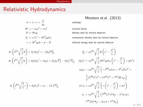
Relativistic Hydrodynamics

Montero et al. (2013)h := 1 + ε +

p

%0

enthalpy

W := −naua = αut Lorentz factor

D := W%0 density seen by normal observer

Si := αTit = W 2

%0hvi momentum density seen by normal observer

τ := W 2%0h − p − D internal energy seen by normal observer

∂t

(e6φ

√γ

γD

)+ ∂j (fD )j = −(fD )j Γkjk f

jD

= αe6φ

√γ

γD

(v i −

βi

α

)

∂t

(e6φ

√γ

γSi

)+ ∂j (fS )i

j = (sS )i + (fS )kj Γkji − (fS )i

k Γjkj

(fS )ij = αe6φ

√γ

γ(W 2

%0hvi

(v j −

βj

α

)+ pδi

j )

(sS )i = αe6φ

√γ

γ

(−T 00

α∂iα + T 0k Diβ

k +

1

2(T 00

βjβk + 2T 0j

βk + T jk )Diγjk

)

∂t

(e6φ

√γ

γτ

)+ ∂j (fτ )j = sτ − (fτ )k Γ

jjk

(fτ )i = αe6φ

√γ

γ

(τ

(v j −

βj

α

)+ pv j

)

sτ = αe6φ

√γ

γ

(T 00(βi

βjKij − β

i∂iα)+

T 0i (2βjKij − ∂iα) + T ijKij

)6 / 273

Spherical polar grids

Spherical polar grids

7 / 273

Spherical polar grids

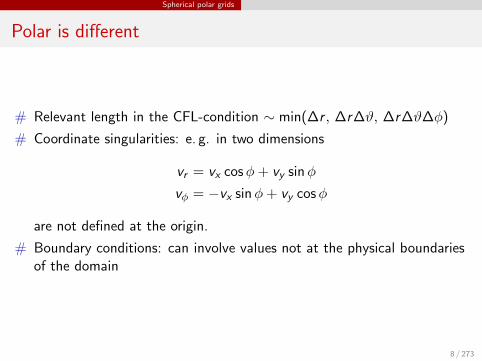
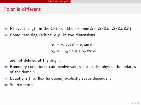
Polar is different

# Relevant length in the CFL-condition ∼ min(∆r , ∆r∆ϑ, ∆r∆ϑ∆φ)

# Coordinate singularities: e. g. in two dimensions

vr = vx cosφ+ vy sinφ

vφ = −vx sinφ+ vy cosφ

are not defined at the origin.

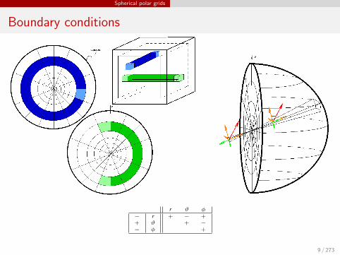
# Boundary conditions: can involve values not at the physical boundariesof the domain

8 / 273

Spherical polar grids

Boundary conditions

r ϑ φ− r + − ++ ϑ + −− φ +

9 / 273

Spherical polar grids

Polar is different

# Relevant length in the CFL-condition ∼ min(∆r , ∆r∆ϑ, ∆r∆ϑ∆φ)

# Coordinate singularities: e. g. in two dimensions

vr = vx cosφ+ vy sinφ

vφ = −vx sinφ+ vy cosφ

are not defined at the origin.

# Boundary conditions: can involve values not at the physical boundariesof the domain

# Equations (i.p. flux functions) explicitly space-dependent

# Source terms

10 / 273

Spherical polar grids

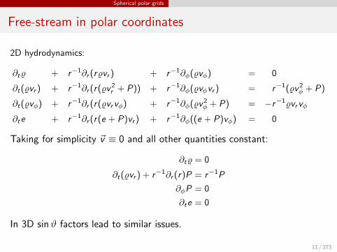
Free-stream in polar coordinates

2D hydrodynamics:

∂t% + r−1∂r (r%vr ) + r−1∂φ(%vφ) = 0

∂t(%vr ) + r−1∂r (r(%v2r + P)) + r−1∂φ(%vφvr ) = r−1(%v2

φ + P)

∂t(%vφ) + r−1∂r (r(%vrvφ) + r−1∂φ(%v2φ + P) = −r−1%vrvφ

∂te + r−1∂r (r(e + P)vr ) + r−1∂φ((e + P)vφ) = 0

Taking for simplicity ~v ≡ 0 and all other quantities constant:

∂t% = 0

∂t(%vr ) + r−1∂r (r)P = r−1P

∂φP = 0

∂te = 0

In 3D sinϑ factors lead to similar issues.

11 / 273

Spherical polar grids

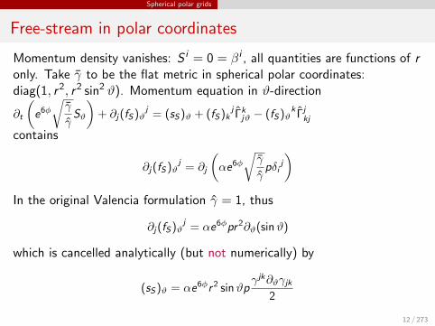
Free-stream in polar coordinates

Momentum density vanishes: S i = 0 = βi , all quantities are functions of ronly. Take γ to be the flat metric in spherical polar coordinates:diag(1, r2, r2 sin2 ϑ). Momentum equation in ϑ-direction

∂t

(e6φ

√γ

γSϑ

)+ ∂j(fS)ϑ

j = (sS)ϑ + (fS)kj Γk

jϑ − (fS)ϑk Γj

kj

contains

∂j(fS)ϑj = ∂j

(αe6φ

√γ

γpδi

j

)In the original Valencia formulation γ = 1, thus

∂j(fS)ϑj = αe6φpr2∂ϑ(sinϑ)

which is cancelled analytically (but not numerically) by

(sS)ϑ = αe6φr2 sinϑpγjk∂ϑγjk

2

12 / 273

Spherical polar grids

Free-stream in polar coordinates

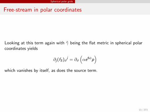
Looking at this term again with γ being the flat metric in spherical polarcoordinates yields

∂j(fS)ϑj = ∂ϑ

(αe6φp

)which vanishes by itself, as does the source term.

13 / 273

Yin-Yang grid

Yin-Yang grid

14 / 273

Yin-Yang grid

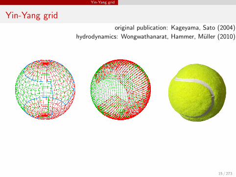
Yin-Yang gridoriginal publication: Kageyama, Sato (2004)

hydrodynamics: Wongwathanarat, Hammer, Muller (2010)

15 / 273

Yin-Yang grid

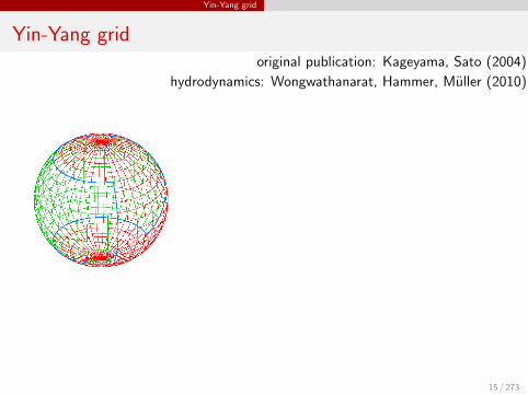
Yin-Yang gridoriginal publication: Kageyama, Sato (2004)

hydrodynamics: Wongwathanarat, Hammer, Muller (2010)

15 / 273

Yin-Yang grid

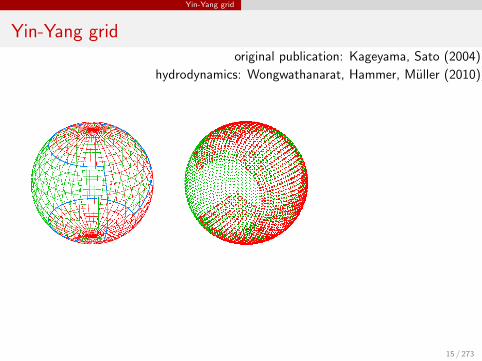
Yin-Yang gridoriginal publication: Kageyama, Sato (2004)

hydrodynamics: Wongwathanarat, Hammer, Muller (2010)

15 / 273

Yin-Yang grid

Yin-Yang gridoriginal publication: Kageyama, Sato (2004)

hydrodynamics: Wongwathanarat, Hammer, Muller (2010)

15 / 273

Yin-Yang grid

Yin-Yang grid

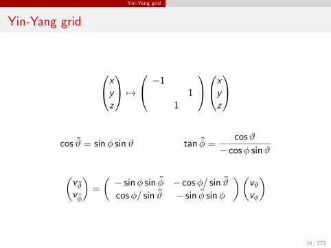
xyz

7→ −1

11

xyz

cos ϑ = sinφ sinϑ tan φ =cosϑ

− cosφ sinϑ

(vϑvφ

)=

(− sinφ sin φ − cosφ/ sin ϑ

cosφ/ sin ϑ − sin φ sinφ

)(vϑvφ

)

16 / 273

Yin-Yang grid

Initial data

Two coordinate systems: two choices of coordinates!

Two examples:

1): Switch from orthonormal to coordinate basis: factors (sinϑ) involvecoordinates of patch.2): Setup of initial data: any functions of ϑ or φ involve only the angles ofthe usual spherical polar coordinate system.

# Note that as the trafo is orthogonal, determinants are unaltered.

# Non-scalar quantities need to be transformed during initialization.

# Axisymmetric setup not possible with a Yin-Yang grid!

17 / 273

Yin-Yang grid

Initial data

Two coordinate systems: two choices of coordinates!

Two examples:1): Switch from orthonormal to coordinate basis: factors (sinϑ) involvecoordinates of patch.

2): Setup of initial data: any functions of ϑ or φ involve only the angles ofthe usual spherical polar coordinate system.

# Note that as the trafo is orthogonal, determinants are unaltered.

# Non-scalar quantities need to be transformed during initialization.

# Axisymmetric setup not possible with a Yin-Yang grid!

17 / 273

Yin-Yang grid

Initial data

Two coordinate systems: two choices of coordinates!

Two examples:1): Switch from orthonormal to coordinate basis: factors (sinϑ) involvecoordinates of patch.2): Setup of initial data: any functions of ϑ or φ involve only the angles ofthe usual spherical polar coordinate system.

# Note that as the trafo is orthogonal, determinants are unaltered.

# Non-scalar quantities need to be transformed during initialization.

# Axisymmetric setup not possible with a Yin-Yang grid!

17 / 273

Yin-Yang grid

Initial data

Two coordinate systems: two choices of coordinates!

Two examples:1): Switch from orthonormal to coordinate basis: factors (sinϑ) involvecoordinates of patch.2): Setup of initial data: any functions of ϑ or φ involve only the angles ofthe usual spherical polar coordinate system.

# Note that as the trafo is orthogonal, determinants are unaltered.

# Non-scalar quantities need to be transformed during initialization.

# Axisymmetric setup not possible with a Yin-Yang grid!

17 / 273

Yin-Yang grid

Boundary and parity conditions

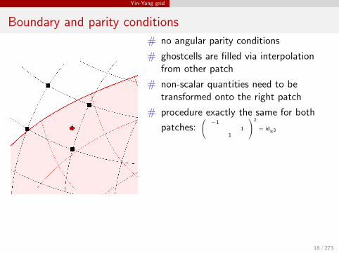
# no angular parity conditions

# ghostcells are filled via interpolationfrom other patch

# non-scalar quantities need to betransformed onto the right patch

# procedure exactly the same for both

patches: −1

11

2

= idR3

# radial boundary / parity unaltered:singularity at r = 0: treated as inBaumgarte at al. (2012) using PIRKschemes

# interpolation may also be needed withradial ghost cells!

But: This is a point-value interpolation!

18 / 273

Yin-Yang grid

Boundary and parity conditions

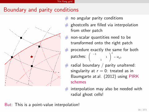
# no angular parity conditions

# ghostcells are filled via interpolationfrom other patch

# non-scalar quantities need to betransformed onto the right patch

# procedure exactly the same for both

patches: −1

11

2

= idR3

# radial boundary / parity unaltered:singularity at r = 0: treated as inBaumgarte at al. (2012) using PIRKschemes

# interpolation may also be needed withradial ghost cells!

But: This is a point-value interpolation!18 / 273

Yin-Yang grid

Yin-Yang grid

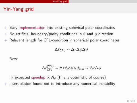
+ Easy implementation into existing spherical polar coordinates

+ No artificial boundary/parity conditions in ϑ and φ direction

+ Relevant length for CFL-condition in spherical polar coordinates:

∆`CFL ∼ ∆r∆φ∆ϑ

Now:

∆`(YY)CFL ∼ ∆r∆φ sinϑmin ∼ ∆r∆φ

⇒ expected speedup ∝ Nϑ (this is optimistic of course)

+ Interpolation found not to introduce any numerical instability

19 / 273

Yin-Yang grid

Yin-Yang grid

− Overlap zones involve interpolations, and for non-scalar quantities alsotransformations

− Overlaps can still not be fully handled without violatingconservativeness of the algorithm

20 / 273

Test problems

Test problems

21 / 273

Test problems

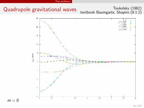
Quadrupole gravitational waves Teukolsky (1982)textbook Baumgarte, Shapiro (9.1.2)

m = 022 / 273

Test problems

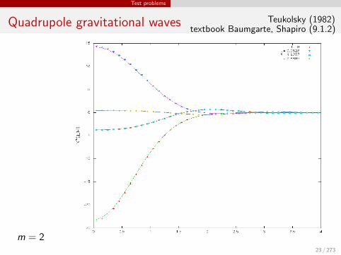
Quadrupole gravitational waves Teukolsky (1982)textbook Baumgarte, Shapiro (9.1.2)

m = 223 / 273

Test problems

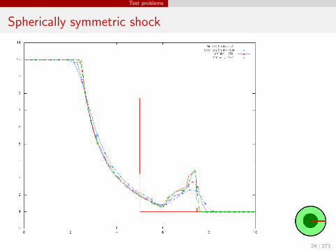
Spherically symmetric shock

24 / 273

Test problems

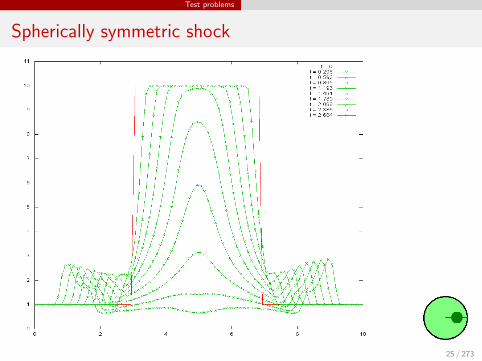
Spherically symmetric shock

25 / 273

Test problems

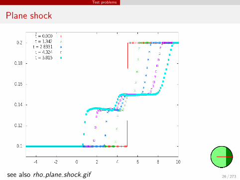
Plane shock

see also rho plane shock.gif 26 / 273

Conclusion

Last slide

Yin-Yang grid

# allows for a reduction of the time step and avoidance of axialsingularities

# needs interpolations and transformations, but is largely based on usualspherical polar coordinates

27 / 273

Conclusion

Thank You!

28 / 273

28 / 273

Alternative form

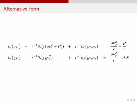
∂t(%vr ) + r−1∂r (r(%v2r + P)) + r−1∂φ(%vφvr ) =

%v2φ

r+

P

r

∂t(%vr ) + r−1∂r (r%v2r ) + r−1∂φ(%vφvr ) =

%v2φ

r− ∂rP

28 / 273

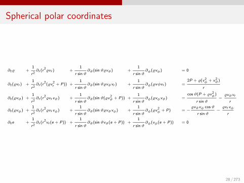
Spherical polar coordinates

∂t% +1

r2∂r (r2

%vr ) +1

r sinϑ∂ϑ(sinϑ%vϑ) +

1

r sinϑ∂φ(%vφ) = 0

∂t (%vr ) +1

r2∂r (r2(%v2

r + P)) +1

r sinϑ∂ϑ(sinϑ%vϑvr ) +

1

r sinϑ∂φ(%vφvr ) =

2P + %(v2φ + v2

ϑ)

r

∂t (%vϑ) +1

r2∂r (r2

%vr vϑ) +1

r sinϑ∂ϑ(sinϑ(%v2

ϑ + P)) +1

r sinϑ∂φ(%vφvϑ) =

cosϑ(P + %v2φ)

r sinϑ−%vϑvr

r

∂t (%vφ) +1

r2∂r (r2

%vr vφ) +1

r sinϑ∂ϑ(sinϑ%vϑvφ) +

1

r sinϑ∂φ(%v2

φ + P) = −%vϑvφ cosϑ

r sinϑ−%vr vφ

r

∂t e +1

r2∂r (r2vr (e + P)) +

1

r sinϑ∂ϑ(sinϑvϑ(e + P)) +

1

r sinϑ∂φ(vφ(e + P)) = 0

28 / 273

Line element

ds2 = dr2 + r2dϑ2 + r2 sin2 ϑdφ2

28 / 273