YiJing Yan and RuiXue Xu - ustc.edu.cnstaff.ustc.edu.cn/~rxxu/14_115.pdf · 25 Feb 2005 21:10 AR AR241-PC56-07.tex XMLPublishSM(2004/02/24) P1: JRX 188 YAN XU quantum information

25 Feb 2005 21:10 AR AR241-PC56-07.tex XMLPublishSM(2004/02/24) P1: JRX10.1146/annurev.physchem.55.091602.094425

Annu. Rev. Phys. Chem. 2005. 56:187–219doi: 10.1146/annurev.physchem.55.091602.094425

Copyright c© 2005 by Annual Reviews. All rights reservedFirst published online as a Review in Advance on December 17, 2004

QUANTUM MECHANICS OF DISSIPATIVE SYSTEMS

YiJing Yan and RuiXue XuDepartment of Chemistry, Hong Kong University of Science and Technology, Kowloon,Hong Kong; email: [email protected]

Key Words non-Markovian dissipation, correlated driving and dissipation,reduced response function, dissipative control

■ Abstract Quantum dissipation involves both energy relaxation and decoherence,leading toward quantum thermal equilibrium. There are several theoretical prescrip-tions of quantum dissipation but none of them is simple enough to be treated exactlyin real applications. As a result, formulations in different prescriptions are practicallyused with different approximation schemes. This review examines both theoreticaland application aspects on various perturbative formulations, especially those that areexact up to second-order but nonequivalent in high-order system-bath coupling con-tributions. Discrimination is made in favor of an unconventional formulation that ina sense combines the merits of both the conventional time-local and memory-kernelprescriptions, where the latter is least favorite in terms of the applicability range of pa-rameters for system-bath coupling, non-Markovian, and temperature. Also highlightedis the importance of correlated driving and disspation effects, not only on the dynamicsunder strong external field driving, but also in the calculation of field-free correlationand response functions.

1. INTRODUCTION

Quantum dissipation refers to the dynamics of a quantum system of primaryinterest in contact with a quantum bath of practically infinite degrees of free-dom. The key theoretical quantity in quantum dissipation is the reduced den-sity operator ρ(t) ≡ trBρT(t), i.e., the partial trace of the total system and bathcomposite ρT(t) over all the bath degrees of freedom. For a system dynamicalvariable A, its expectation value, A(t) = Tr[AρT(t)] = tr[Aρ(t)], can therefore beevaluated with the substantially reduced system degrees of freedom. Quantum dis-sipation theory governs the evolution of the reduced density operator ρ(t), wherethe effects of bath are treated in a quantum statistical manner. It thus providesnot just the aforementioned numerical advantage, but also the irreversibility ofquantum statistical mechanics.

Because of its fundamental importance in almost all fields of modern science,quantum dissipation theory has remained as an active topic of research since aboutthe middle of the past century. Its development involved scientists working infields as diversified as nuclear magnetic resonance (1–4), quantum optics (5–13),

0066-426X/05/0505-0187$20.00 187

25 Feb 2005 21:10 AR AR241-PC56-07.tex XMLPublishSM(2004/02/24) P1: JRX

188 YAN � XU

quantum information and quantum measurement (14, 15), solid-state physics andmaterial science (16–18), mathematical physics (19–23), nonlinear spectroscopy(24–34), and statistical dynamics and chemical physics (35–68).

The challenge here arises from the combined effects of strong system-bath in-teraction, non-Markovian dissipation, and time-dependent external driving. Thesecombined effects can be incorporated in a formally exact manner via the Feynman-Vernon influence functionals of path integral formalism (35–37). Numericallyexact methods for the path integral formalism, such as quantum Monte Carlo tech-niques combined with iterative forward-backward propagation schemes (69–71),have set up the benchmark to investigate non-Markovian dynamics beyond theweak system-bath interaction regime. The integral formalism is, however, neithernumerically practical for realistic systems nor theoretically tractable for furtherconstruction of such as nonlinear spectroscopy formulations.

This review considers the differential formalism of quantum dissipation the-ory, abbreviated hereafter as QDT, which is also often termed as quantum masterequations in literature. The present review focuses on some second-order QDT for-mulations in terms of their constructions and applicabilities, and sheds light partic-ularly on the implication of the correlation between non-Markovian dissipation andexternal time-dependent field drive. The high-order perturbative formulations areusually too complicated for general purpose (72–74). The canonical transformationmethods can effectively reduce the system-bath coupling strength via consideringthe transformed reduced system such as polaron (17, 18) or including the solvationmodes into explicit consideration. Readers may refer to, for example, Reference52 on this topic. Semiclassical methods (75–87) where it would be practical toinclude the strong system-bath coupling effects are not included in this review.

We note that there has recently been an increasing interest in stochastic Hilbert-and/or Liouville-space dynamics that unravels the reduced description (11, 12,88–92). Quantum stochastic description provides not only numerical methods onreduced dynamics propagations (89, 90) but also powerful tools for the constructionof exact QDT formulations (91–94). Stochastic interpretation is also closely relatedto continuous quantum measurements (14, 15). Readers may refer to Reference88, for example, for the details of stochastic quantum dissipation.

Throughout this review, h ≡ 1 and β ≡ 1/(kBT ) for simplicity, where kB is theBoltzmann constant and T the temperature.

2. BACKGROUND OF NONEQUILIBRIUM QUANTUMSTATISTICAL MECHANICS

In this section, we review some background on the (two-time) correlation func-tion and response function that arise from linear response theory. We discuss thesymmetry, detailed-balance, and fluctuation-dissipation relations implied there.The importance of correlation/response functions to nonequilibrium statisticalmechanics is similar to that of partition functions to equilibrium statistical


QUANTUM MECHANICS OF DISSIPATIVE SYSTEMS 189

mechanics. Correlation/response functions have been widely used in the study ofphysical problems such as spectroscopy (24–34), transport (38–43), and reactionrate (68, 95–97).

2.1. Correlation and Response Functions VersusLinear Response Theory

Consider the measurement on a dynamical variable A with a classical probefield ε(t) that couples with the system as −Bε(t). For simplicity, both operatorsA and B are assumed to be Hermite. The total composite material system wasinitially at the thermal equilibrium, ρeq

M = e−β HM/Tre−β HM , before external fielddisturbance. The field-induced deviation in A(t) from its equilibrium expectationvalue is δ A(t) = Tr{A[ρT(t) − ρ

eqM ]}, where ρT(t) is the total composite system

density operator in the presence of external field. To the first order of the externaldisturbance, we have

δ A(t) =t∫

−∞dτχAB(t − τ )ε(τ ), 2.1.

with the material response function given by

χAB(t − τ ) ≡ i〈[A(t), B(τ )]〉M. 2.2.

Here, [. . ., . . .] denotes a commutator, O(t) ≡ ei HMt Oe−i HMt , and 〈. . .〉M ≡Tr(. . . ρeq

M ). Physically, the response function χAB(t) is needed only for t ≥ 0 due tocausality (cf. Equation 2.1). Its extension to t < 0 is formally made with Equation2.2 as

χAB(−t) = −χBA(t). 2.3.

Obviously, the response function χAB(t) for Hermitian operators is real.We now turn to the correlation function, denoted as

CAB(t − τ ) ≡ 〈A(t)B(τ )〉M. 2.4.

Either χAB(t − τ ) of Equation 2.2 or CAB(t − τ ) of Equation 2.4 depends only onthe duration t − τ . This is a property of the stationary statistics as [HM, ρ

eqM ] = 0.

We have also that 〈A(t)〉M = 〈A〉M, which does not depend on time, and

〈 A(t)B(0)〉M = −〈A(t)B(0)〉M. 2.5.

Moreover, the correlation function satisfies the following symmetry and detailed-balance relations:

C∗AB(t) = CBA(−t) = CAB(t − iβ). 2.6.

Note that χAB(t) = −2ImCAB(t). The common phenomenon of statistical indepen-dence as t → ∞ implies that CAB(t → ∞) = 〈A〉M〈B〉M in a general dissipative


190 YAN � XU

system. One may remove this nonzero asymptotic value by setting A − 〈A〉M

and B −〈B〉M as new variables and consider only the shifted correlation functionsthat satisfy CAB(t → ∞) = 0.

2.2. Spectrum and Dispersion FunctionsVersus Kramers-Kronig Relations

Let us now introduce the so-called causality transformation via

CAB(ω) ≡∞∫

0

dt eiωt CAB(t). 2.7.

Here, CAB(t → ∞) = 0 is implied. The generalized spectrum CAB(ω) and disper-sion DAB(ω) functions, by which

CAB(ω) = CAB(ω) + i DAB(ω), 2.8.

can then be defined, respectively, as

CAB(ω) ≡ 1

2[CAB(ω) + C∗

BA(ω)] = 1

2

∞∫−∞

dt eiωt CAB(t) = C∗BA(ω) and 2.9a

DAB(ω) ≡ 1

2i[CAB(ω) − C∗

BA(ω)] = D∗BA(ω). 2.9b

Thus, Equation 2.8 represents the separation of Hermite and anti-Hermite compo-nents rather than that of real and imaginary parts.

An important mathematical property implied in the causality transform Equa-tion 2.7 is that CAB(z) is an analytical function in the upper plane (Imz > 0). Byusing the contour integration formalism, together with the identity 1/(ω′ − ω) =P{1/(ω′ − ω)} + iπδ(ω′ − ω), we have

CAB(ω) = i

πP

∞∫−∞

dω′ CAB(ω′)ω − ω′ . 2.10.

Here,P denotes the principle part. This is the Kramers-Kronig relation, which canbe recast as

CAB(ω) = − 1

πP

∞∫−∞

dω′ DAB(ω′)ω − ω′ , DAB(ω) = 1

πP

∞∫−∞

dω′ CAB(ω′)ω − ω′ . 2.11.

Similarly, the causality transform of the response function is

χAB(ω) ≡∞∫

0

dteiωtχAB(t) = χ(+)AB (ω) + i χ (−)

AB (ω), 2.12.



where χ(+)AB (ω) = [χ (+)

BA (ω)]∗ and χ(−)AB (ω) = [χ (−)

BA (ω)]∗ are the Hermite and anti-Hermite components, respectively. They also satisfy the aforementioned Kramers-Kronig relations.

Using Equations 2.2, 2.7, 2.8 and 2.12, we obtain

χ(+)AB (ω) = −[DAB(ω) + DBA(−ω)], 2.13a.

χ(−)AB (ω) = CAB(ω) − CBA(−ω) = 1

2i

∞∫−∞

dt eiωtχAB(t). 2.13b.

It then follows that, χ (+)AB (−ω) = χ

(+)BA (ω) and χ

(−)AB (−ω) = −χ

(−)BA (ω). As described

in Equation 2.13b, {χ (−)AB (ω)} is also termed the spectral density function.

2.3. Fluctuation-Dissipation Theorem

The detailed-balance relation in terms of spectrum functions reads as

CBA(−ω) = e−βωCAB(ω). 2.14.

Together with the first identity of Equation 2.13b, we have

χ(−)AB (ω) = (1 − e−βω)CAB(ω). 2.15.

This relation is called the fluctuation-dissipation theorem (FDT). It can be recastas

CAB(t) = 1

π

∞∫−∞

dωe−iωt χ

(−)AB (ω)

1 − e−βω. 2.16.

It thus also establishes the relation between the correlation function CAB(t) and theresponse function χAB(t) (cf. Equation 2.13b). The FDT is a result of the detailed-balance relation.

In Appendix A, the FDT is applied to formulate the equilibrium phase-spacevariances, σ eq

qq ≡ 〈q2〉 − 〈q〉2 and σeqpp ≡ 〈p2〉 − 〈p〉2, in terms of the coordinate

response function χqq (t) for arbitrary one-dimensional systems. Some additionalproperties in relation to the spectrum and/or spectral density functions are sum-marized as follows.

It is easy to show that not just CAA(ω) ≥ 0, but also CAA(ω)CB B(ω) ≥ |CAB(ω)|2,for all real ω. In fact, the Hermitian matrix {CAB(ω)} of spectrum functions is ofcomplete positivity (60, 98). It leads also to the positivity of spectral density{χ (−)

AB (ω)} for ω ≥ 0 as inferred from Equation 2.15.


192 YAN � XU

We have also the following expressions,

χAB(0) = 1

π

∞∫−∞

dωχ

(−)AB (ω)

ω, χAB(0) = 1

π

∞∫−∞

dω ωχ(−)AB (ω). 2.17.

The first expression is obtained when the Kramer-Kronig relation is at zero fre-quency, together with χ

(+)AB (0) = χAB(0) as inferred from Equation 2.15 that

χ(−)AB (0) = 0. Note that as χAB(t) is real for Hermite operators, χAB(0) must be

real (cf. Equation 2.12). The second expression in Equation 2.17 is obtained bytaking the time derivative of the inverse Fourier transform of Equation 2.13b,followed by setting t = 0.

Later in this review, the bath correlation/response functions for a set of bathoperators {Fa(t) ≡ eihBt Fae−ihBt } will be exploited to describe the energy relax-ation and decoherence processes in the reduced system of primary interest. Thebath correlation functions will be denoted similarly as

Cab(t) ≡ trB[Fa(t)Fb(0)ρeqB ] ≡ 〈Fa(t)Fb(0)〉B. 2.18.

However, the bath response functions χab(t) will be renamed as

φab(t) ≡ i〈[Fa(t), Fb(0)]〉B, 2.19.

to avoid possible confusions that may occur there. The bath spectral density functi-ons φ

(−)ab (ω) [or χ

(−)ab (ω)] will further be renamed as Jab(ω). Clearly, all relations

presented earlier in this section remain valid for the bath correlation/responsefunctions. For example, the FDT of Equation 2.16 now reads as

Cab(t) = 1

π

∞∫−∞

dωe−iωt Jab(ω)

1 − e−βω. 2.20.

The generalized frictional function γab(t) can also be introduced via

φab(t) ≡ −γab(t) or φab(ω) = γab(0) + iωγab(ω). 2.21.

Note that γab(t) = γba(−t). The first expression in Equation 2.17 is now

γab(0) = φab(0) = 1

π

∞∫−∞

dωJab(ω)

ω. 2.22.



3. EXACT DYNAMICS OF DRIVENBROWNIAN OSCILLATORS

This section discusses an exactly solvable model, the driven Brownian oscillator(DBO) systems (36, 37, 60, 99, 100). It also highlights some issues on the generalQDT formulation.

3.1. Model and Quantum Langevin Equations

Let us start with the total composite Hamiltonian in the presence of external clas-sical field drive, HT(t) ≡ HM + Hsf(t). In the DBO model, the system-field inter-action assumes Hsf(t) = −qε(t), and the total field-free system-plus-bath materialHamiltonian assumes the Calderia-Leggett form (50, 51)

HM =(

p2

2M+ 1

2M�2

0q2

)+

∑j

[p2

j

2m j+ 1

2m jω

2j

(x j − c j

m jω2j

q)2

]. 3.1.

The last term here contains the free-bath hB = ∑j [p2

j/(2m j ) + m jω2j x

2j /2], the

system-bath {q · x j }-coupling, and the coupling-induced renormalization Hren thatdepends only on the DBO’s degree of freedom. Thus,

HM = H0 + Hren + hB −√

M q F ≡ Hs + hB −√

M q F. 3.2.

The mass-scaled Langevin force, F = f/√

M = ∑j c j x j/

√M , is adopted to

satisfy the relation in Equation 2.21, i.e.,

φ(t) ≡ i〈[F(t), F(0)]〉 = −γ (t) or φ(ω) = γ (0) + iωγ (ω). 3.3.

Here, F(t) = eihBt Fe−ihBt and γ (t) assumes the classical frictional function,

γ (t) = 1

M

∑j

c2j

m jω2j

cos(ω j t). 3.4.

In Equation 3.2, H0 is given by the first term in Equation 3.1 with frequency �0,and

Hs ≡ H0 + Hren = p2

2M+ 1

2M�2

Hq2, 3.5.

with

�2H ≡ �2

0 + 1

M

∑j

c2j

m jω2j

= �20 + γ (0). 3.6.

We shall later show that �0, rather than �H, represents the DBO frequency in theMarkovian white-noise limit. However, in general the DBO frequency appears asneither �0 nor �H.


194 YAN � XU

The quantum Langevin equations for the DBO system can easily be derivedvia the Heisenberg equations of motion with HT(t) = HM − qε(t). By using theformal solutions of bath degrees of freedom, we obtain

˙q(t) = p(t)/M, 3.7a

˙p(t) = −M�2Hq(t) + M

t∫t0

dτφ(t − τ )q(τ ) + ε(t) + fB(t)

= −M�20q(t) −

t∫t0

dτγ (t − τ ) p(τ ) + ε(t) + fB(t). 3.7b

Here fB(t) ≡ √M F(t) is the standard quantum Langevin force operator. The

second identity of Equation 3.7b is the conventional form of the Langevin equa-tion, obtained by performing the integration by part, together with Equations 3.3and 3.6.

3.2. Quantum Master Equation

The formal solution to Equations 3.7 is given by (60)

[q(t)

p(t)

]= T(t − t0)

[q(t0)

p(t0)

]+

t∫t0

dτT(t − τ )

[0

ε(τ ) + fB(τ )

], 3.8.

with

T(t) =[

χpq (t) χqq (t)

−χpp(t) χpq (t)

]≡

[Mχ (t) χ (t)

M2χ (t) Mχ (t)

]. 3.9.

Here, χAB(t) (Equation 2.2) denotes the conventional response function in the totalcomposite material HM-space. In the second identity of Equation 3.9, we made useof Equation 2.5 and χ (t) ≡ χqq (t), which will be specified later in terms of bathresponse or frictional function (cf. Equations 3.13–3.15).

Equation 3.8 may be used to construct an exact quantum master equation via,for example, the Yan-Mukamel method based on the Gaussian wave packet dy-namics in the Wigner phase space (26, 60). However, as pointed out by Karrlein &Grabert (100), there does not exit a generally exact QDT for arbitrary initial bathpreparations.

In this review, we shall focus on the reduced dynamics induced by the externalfield. The natural initial condition to be adopted acquires the thermal equilibriumstate for the total composite material system, ρT(t0) = ρ

eqM , before the external field

interaction. The initial time can thus be set to t0 → −∞.



The exact quantum master equation for the DBO system is summarized asfollows (60):

ρ(t) = −i

[p2

2M+ 1

2M�2q2 − qεeff(t), ρ(t)

]− i

2γ [q, {p, ρ(t)}]

− γ σ eqpp[q, [q, ρ(t)]] − (

σ eqpp/M − M�2σ eq

qq

)[q, [p, ρ(t)]]. 3.10.

Here, ( [. . ., . . .] denotes a commutator and {. . ., . . .} an anticommutator)

� ≡ limt0→−∞ �t−t0 , γ ≡ lim

t0→−∞ γt−t0 , 3.11a.

with

�2t = χ2(t) − ···χ(t)χ (t)

χ2(t) − χ (t)χ (t), γt =

···χ (t)χ (t) − χ (t)χ (t)

χ2(t) − χ (t)χ (t), 3.11b.

and

εeff(t) = ε(t) +t∫

t0

dτχε(t, τ )ε(τ ), 3.12a.

with

χε(t, τ ) ≡ M[�2χ (t − τ ) + γ χ (t − τ ) + χ (t − τ )]. 3.12b.

The thermal equilibrium phase-space variances, σ eqqq and σ

eqpp, involved in Equation

3.10 are given by Equation A.1 or A.3 in terms of the causality transform of χ (t).In deriving Equation 3.10, the determinant |T(t)| of the transfer matrix in Equa-

tion 3.9 is assumed nonzero; otherwise both �t and γt diverge (Equations 3.11).Equation 3.10 recovers the well-established result (100) by setting ε(t) = 0 andreplacing � and γ with �t and γt as the initial time of t0 = 0 was adopted in theirwork.

The key quantity here is the well-established Brownian response function χ (t) ≡χqq (t). With the linear response theory being applied for Equations 3.7, one canreadily obtain that (cf. Equations 3.3 and 3.6)

χ (t) + �2Hχ (t) −

t∫0

dτφ(t − τ )χ (τ ) = 0, 3.13a.

or equivalently

χ (t) + �20χ (t) +

t∫0

dτγ (t − τ )χ(τ ) = 0. 3.13b.

From its definition, Equation 2.5, and Equation 3.13, we have

χ (0) = χ (0) = 0, χ (0) = −···χ (0)/�2H = 1/M. 3.14.


196 YAN � XU

Therefore (cf. Equation 3.3)

χ (ω) = 1/M

�2H − ω2 − φ(ω)

= 1/M

�20 − ω2 − iωγ (ω)

. 3.15.

3.3. Comments

The correlated driving-dissipation effect on the reduced DBO dynamics is de-scribed by the second term in the right-hand side of Equation 3.12a as an effectivefield correction. This correlated effect is completely coherent in the present case.In a general anharmonic system, the correlated driving and dissipation effects areusually quite complicated. We shall come back to this point below.

In the Markovian white-noise limit, γ (t) = 2γmarδ(t) or γ (ω) = γmar is a con-stant. In this limit, Equations 3.15, 3.11 and 3.12 reduce, respectively, to

χ (t) → sin[(

�20 − γ 2

mar/4) 1

2 t]

M(�2

0 − γ 2mar/4

) 12

e−γmart/2, 3.16a.

�t → �0, γt → γmar, 3.16b.

χε(t, τ ) = 0, εeff(t) = ε(t). 3.16c.

The effects of the driving and dissipation correlation, due to δεeff(t) ≡ εeff(t) − ε(t)in the DBO system, vanish completely in the Markovian limit. The δ(t)-noise is ill-defined for short time; it causes σ

eqpp to diverge (Equation A.3). However, analysis of

the white-noise limit is instructive; it implies that H0 would rather be the choice ofthe reduced system Hamiltonian if a phenomenological description of dissipationwere to be adopted. For example, σ eq

qq and σeqpp may be replaced with their zeroth-

order values σ 0qq and σ 0

pp in the pure-H0 system, and approximate Equation 3.10as (55)

ρ(t) → −i[H0 − qε(t), ρ(t)] − i

2γ [q, {p, ρ(t)}] − γ σ 0

pp[q, [q, ρ(t)]]. 3.17.

The last term in Equation 3.10 becomes zero in this phenomenological description.Note that � and γ serve as the frequency and friction constants entering into

Equation 3.10, and they are the long-time asymptotic values of �t and γt as de-scribed by Equations 3.11. Clearly, �t=0 = �H and γt=0 = 0 as inferred fromEquation 3.14. In strong non-Markovian interaction regime, �t ( �) and γt ( γ )may diverge. One may argue that � and γ could be treated phenomenologicallyas the Markovian parameters in Equation 3.10. However, the non-Markovian na-ture of Equation 3.10 still remains as εeff(t) = ε(t). As mentioned earlier, thisinequality characterizes the correlated driving-dissipation effects in the presentcase. We shall see later that for a general system the field-free dissipation could becharacterized by a Markovian-like, time-independent dissipative superoperator, asthe system was initially in the thermal equilibrium state before the external field



excitation. The dynamical non-Markovian effects enter only through the field-dressed dissipative superoperator component.

4. TWO PRESCRIPTIONS OF QUANTUMDISSIPATION THEORY

4.1. General Description of Total Composite Hamiltonian

The total composite Hamiltonian in the presence of classical external field can bewritten as

HT = HM + Hsf(t) ≡ Hs + Hsf(t) + hB −∑

a

Qa Fa . 4.1.

The last term in Equation 4.1 describes the system-bath couplings, in which {Qa}are Hermite operators of the primary system and can be called the generalizeddissipative modes. The generalized Langevin forces {Fa(t) ≡ eihBt Fae−ihBt } areHermite bath operators in the stochastic bath subspace assuming Gaussian statis-tics. Without loss of generality, their stochastic mean values are set to 〈Fa(t)〉B = 0.The effects of Langevin forces on the reduced primary system are thereforecompletely characterized by their correlation functions Cab(t) = 〈Fa(t)Fb(0)〉B(Equation 2.18), or other equivalent properties, such as the generalized frictionalfunctions γab(t), described in Section 2. For the later construction of coupled differ-ential equations of motion, we adopt the extended Meier-Tannor parameterizationmodel that, as detailed in Appendix B, leads the bath correlation functions to thefollowing form (57, 60, 61):

Cab(t ≥ 0) =m∑

m=0

νabm tδm0 e−ζ ab

m t ; with ζ ab0 ≡ ζ ab

1 . 4.2.

In Equation 4.1, the reduced system Hamiltonian in the presence of externalclassical field is

H (t) ≡ Hs + Hsf(t) ≡ H0 + Hren + Hsf(t). 4.3.

Here, Hs is the time-independent, field-free Hamiltonian, whereas Hsf(t) is theinteraction between the system and the external classical field ε(t). The Calderia-Leggett form of renormalization Hamiltonian assumes Hren = 1

2

∑γab(0)Qa Qb

(cf. Equation 3.6). As discussed in Section 3, it is H0, rather than Hs , that resem-bles the effective system Hamiltonian to be observed in the high temperature orMarkovian limit. The result is that H0 is adopted as the reduced field-free systemHamiltonian in some phenomenological QDT formulations that also assume thethermal equilibrium reduced state of ρeq ∝ e−β H0 . Further discussion on the issuewill be made in the last paragraph of Section 4.2.

The theory presented below goes beyond the phenomenological level, where Hs

enters as the reduced field-free system Hamiltonian. Both the reduced dynamics


198 YAN � XU

and the reduced thermal canonical state should be evaluated with dissipation. Forlater use, let us denote the following Liouvillians,

L(t)O ≡ [H (t), O], Ls O ≡ [Hs, O], Lsf(t)O ≡ [Hsf(t), O]. 4.4.

The coherent propagatorG(t, τ ) associating withL(t) is defined via

∂

∂tG(t, τ ) ≡ −iL(t)G(t, τ ). 4.5.

It is equivalent toG(t, τ )O = G(t, τ )OG†(t, τ ), where G(t, τ ) is the Hilbert-spacepropagator with ∂t G(t, τ ) = −i H (t)G(t, τ ). The field-free counterpart is denotedasGs(t, τ ), which is given by

Gs(t, τ ) = e−iLs ·(t−τ ) ≡ Gs(t − τ ). 4.6.

4.2. Perturbative Formulations in Two Prescriptions

There are two commonly used prescriptions of QDT. One is characterized by amemory dissipation kernel ϒ(t, τ ) and reads as follows (39–42):

ρ(t) = −iL(t)ρ(t) −t∫

−∞dτϒ(t, τ )ρ(τ ). 4.7.

According to the temporal sequence of the involving actions in ϒ(t, τ )ρ(τ ), Equa-tion 4.7 is also said to be in the chronological ordering prescription (COP). Analternative prescription of the QDT is characterized by a time-local dissipationkernelR(t) and reads (43)

ρ(t) = −iL(t)ρ(t) − R(t)ρ(t). 4.8.

According to the temporal sequence of the involving actions inR(t)ρ(t), Equa-tion 4.8 is also said to be in a partial ordering prescription (POP) in contrast toEquation 4.7. In principle, both ϒ(t, τ ) andR(t) can be formulated exactly byusing, for example, the Nakajima-Zwanzig-Mori projection operator techniques(39–43). In this sense, Equation 4.7 and Equation 4.8 are equivalent. However,the exact QDT in the forms of differential equations of motion (EOM) are by farnumerically tractable in very few systems, such as the DBO system (describedin Section 3) and the spin-boson system (89, 101, 102). In most cases, certainapproximation schemes are employed.

Let us consider the weak system-bath interaction regime and focus on a so-called complete second-order quantum dissipation theory (CS-QDT). Here, thesystem-bath couplings are rigorously accounted for to second order, not only for thedynamics of ρ(t), but also for the initial reduced canonical state ρ(t0) = trBρ

eqM (T );

this includes the nonfactorizable ρeqM (T ), before external field excitation. Various

forms of CS-QDT are the same at the second order system-bath interaction level,but differ at their partial resummation schemes in approximating higher order



contributions. In this review, we shall discuss three nonequivalent forms of CS-QDT. Two of them resemble Equations 4.7 and 4.8, and will be presented later inthis section as the COP-CS-QDT and the POP-CS-QDT, respectively. The thirdone is nonconventional and will be discussed in detail in the next section.

A perturbative QDT can be formulated by some relatively simple methodswithout explicitly invoking the Nakajima-Zwanzig-Mori projection operator tech-niques (4–8, 38, 52–57, 59). By using explicitly the decomposite form of system-bath couplings as shown in the last term of Equation 4.1, the COP-CS-QDT ofEquation 4.7 can be readily obtained, where (57, 59)

t∫−∞

dτϒ(t, τ )ρ(τ ) =∑

a

{[Qa, Qcop

a (t)] + H.c.

}, 4.9a.

with

Qcopa (t) =

∑b

t∫−∞

dτ Cab(t − τ )G(t, τ )[Qbρ(τ )], 4.9b.

and the POP-CS-QDT of Equation 4.8, where (23, 59)

R(t)ρ(t) =∑

a

{[Qa, Qpop

a (t)ρ(t)] + H.c.

}, 4.10a.

with

Qpopa (t) =

∑b

t∫−∞

dτ Cab(t − τ )G(t, τ )Qb. 4.10b.

To investigate the correlated driving-dissipation effects involved here, we makeuse of the following identity,

G(t, τ ) = Gs(t, τ ) − i

t∫τ

dτ ′G(t, τ ′)Lsf(τ′)Gs(τ ′, τ ). 4.11.

In particular, we can recast Equation 4.10b as

Qpopa (t) = Qa −i

∑b

t∫−∞

dτ

t∫τ

dτ ′Cab(t −τ )G(t, τ ′)Lsf(τ′)Gs(τ ′−τ )Qb, 4.12.

with

Qa ≡∑

b

t∫−∞

dτ Cab(t − τ )e−iLs (t−τ ) Qb =∑

b

Cab(−Ls)Qb. 4.13.


200 YAN � XU

Here, Cab(−Ls) is a reduced Liouville-space operator, defined by the field-freeLiouvillianLs and the causality spectrum Cab(ω) of the bath correlation function.The field-free dissipation in the POP-CS-QDT is therefore characterized by thetime-independentRs , with (cf. Equation 4.10a)

Rsρ(t) ≡∑

a

[Qa, Qaρ(t) − ρ(t)Q†a]. 4.14.

Similarly, the field-free dissipation in the COP-CS-QDT is characterized by thememory kernel of ϒs(t − τ ), which is defined similarly as Equations 4.9 but withtheG(t, τ ) in Equation 4.9b replaced byGs(t, τ ) = e−iLs ·(t−τ ).

To conclude this subsection, let us make some comments on the non-Markoviannature of a QDT. Traditionally, a QDT characterized by a time-independentRs

would be classified as Markovian, whereas a QDT characterized by a memorykernel ϒs(t −τ ) would be classified as non-Markovian. However,Rs and ϒs(t −τ )are equivalent at the field-free CS-QDT level and both of them can describe colorednoises. In the white-noise limit, the field-free COP assumes

t∫−∞

dτϒs(t − τ )ρ(τ ) → Rmarρ(t), 4.15.

where

Rmarρ(t) ≡∑a,b

[Qa, Cab(−Ls){Qbρ(t)}] + H.c. 4.16.

Clearly,Rs = Rmar. This implies that classifying theRs-based CS-QDT as Marko-vian is due to the lack of driving-dissipation cooperativity rather than to the natureof bath. In fact, non-Markovian nature enters into the reduced equilibrium densityoperator ρ

popeq of theRs-based CS-QDT, but does not enter into its ϒs(t − τ )-based

counterpart ρcopeq (cf. Section 4.4).

It is worth mentioning here that in some phenomenological quantum masterequations, the reduced equilibrium state is set to be independent of dissipation,together with the neglect of correlated driving and dissipation effects. In this case,the phenomenological QDT would read (55)

ρ(t) → −i[H0 + Hsf(t), ρ(t)] −∑a,b

{[Qa, {Cab(−L0)Qb}ρ(t)] + H.c.}. 4.17.

Here, H0 = Hs − Hren was given in Equation 4.3, and only the bath spectrumfunctions {Cab(ω)} are involved. The effects of bath dispersions {Dab(ω)} are phe-nomenologically incorporated into the coupling-induced renormalization contri-bution to the reduced system Hamiltonian. It can easily show that Equation 4.17assumes the equilibrium state of ρ0

eq ∝ e−β H0 (55). Equation 4.17 recovers Equa-tion 3.17 in the DBO system. As discussed in Section 3.3, the phenomenologicalQDT (Equation 4.17) does amount to a Markovian formulation (cf. Appendix Dof Reference 59).



4.3. Differential Equations of Motion

With the model bath of Equation 4.2, the COP-CS-QDT and the POP-CS-QDTpresented in Section 4.2 can further be expressed in terms of closed sets ofdifferential EOM. Let us start with the COP-CS-QDT (Equations 4.7 and 4.9).We have

Qcopa (t) ≡

m∑m=0

∑b

νabm K cop

m,ab(t), 4.18.

where

K copm,ab(t) ≡

t∫−∞

dτ (t − τ )δm0 e−ζ abm (t−τ )G(t, τ )[Qbρ(τ )]. 4.19.

Note that ζ ab0 = ζ ab

1 . The final EOM for COP-CS-QDT read (60)

ρ(t) = −iL(t)ρ(t) −∑m,a,b

{νab

m

[Qa, K cop

m,ab(t)] + H.c.

}, 4.20a.

K copm,ab(t) = δm0 K cop

1,ab(t) + (1 − δm0)Qbρ(t) − [iL(t) + ζ ab

m

]K cop

m,ab(t). 4.20b.

The natural initial conditions to the above coupled set of EOM are

ρ(t0) = ρcopeq and K cop

m,ab(t0) = (iLs + ζ ab

m

)−(δm0+1)(Qbρ

copeq

). 4.21.

Here, t0 can be any time before the external field acts. The COP reduced thermalequilibrium density operator ρ

copeq will be discussed in Section 4.4.

We now turn to the POP-CS-QDT (Equations 4.8 and 4.10). Let Equation 4.12be recast as

Qpopa (t) ≡ Qa + δ Qpop

a (t). 4.22.

Here, δ Qpopa (t) is given by the second term of Equation 4.12, which together with

Equation 4.2 can be expressed as

δ Qpopa (t) =

m∑m=0

∑b

νabm K pop

m,ab(t), 4.23.

with (noting that ζ ab0 = ζ ab

1 )

K popm,ab(t) = −i

t∫−∞

dτ

t∫τ

dτ ′ (t − τ )δm0 e−ζ abm (t−τ )

×G(t, τ ′)Lsf(τ′)Gs(τ

′ − τ )Qb. 4.24.


202 YAN � XU

The final EOM for POP-CS-QDT therefore read (60)

ρ(t) = −iL(t)ρ(t) − Rsρ(t) −∑m,a,b

{νab

m

[Qa, K pop

m,ab(t)ρ(t)] + H.c.

}, 4.25a.

K popm,ab(t) = δm0 K pop

1,ab(t) − [iL(t) + ζ ab

m

]K pop

m,ab(t) − i[Hsf(t), Qab

m

]. 4.25b.

HereRs was given by Equation 4.14, and the ordinary operator Qabm (t) in the

inhomogeneous term in Equation 4.25b is

Qabm ≡ (

iLs + ζ abm

)−(δm0+1)Qb. 4.26.

Note that the EOM for K popm,ab(t) is independent, except for K pop

0,ab(t) that couplesalso to K pop

1,ab(t). The initial conditions to Equations 4.25 are ρ(t0) = ρpopeq , which

will be discussed later, and K popm,ab(t0) = 0 for m ≥ 0.

4.4. Evaluation of Reduced Canonical States

The reduced canonical equilibrium density operator applies for both the initialand the asymptotic states before and after the external field excitation. It can beevaluated via the field-free propagation for long time as ρeq = ρ(t → ±∞).Alternatively, ρeq can be evaluated via the nondynamical approach by consideringthe stationary condition for the field-free version of QDT, which in the POP-CS-QDT assumes

ρpopeq = −(iLs + Rs)ρ

popeq = 0. 4.27.

The details of evaluation of ρpopeq are presented in Appendix C. Similarly, we have

(cf. Equations 4.7 and 4.9)

ρcopeq = −(iLs + Rmar)ρ

copeq = 0. 4.28.

Here,Rmar describes the white-noise Markovian limit of dissipation (Equation4.16). Therefore, ρcop

eq is identical to its Markovian counterpart! It is in contrastwith ρ

popeq in Equation 4.27, and implies that the time-independentRs does physi-

cally describe certain non-Markovian effects at least on the equilibrium properties.To demonstrate the points raised above, let us consider the DBO system and

compare ρpopeq and ρ

copeq with respect to the exact ρex

eq . Depicted in Figure 1 are theresults of the reduced phase-space variances σqq and σpp as functions of tempera-ture. Note that both ρex

eq and ρpopeq are Gaussian wave packets in the reduced phase

space (cf. Appendix D); thus they are completely described by the variances shownin Figure 1 as their 〈q〉eq, 〈p〉eq, and 〈pq + qp〉eq are all zero values. Appendix Dalso explicitly shows that both the exact DBO propagator and its POP-CS-QDTcounterpart are Gaussian and preserve positivity. The COP-CS-QDT does not havethese properties. The non-Gaussian ρ

copeq (T ) starts to violate the positivity even at

a moderately low temperature, which is kBT/�0 ≈ 0.7 (checked against the un-certainty principle) in the case under study in Figure 1.



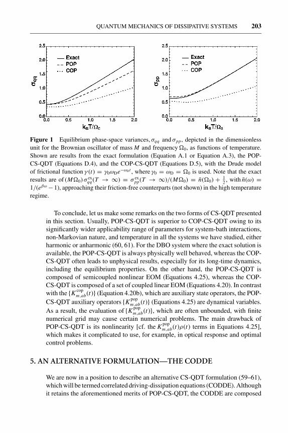
Figure 1 Equilibrium phase-space variances, σqq and σpp, depicted in the dimensionlessunit for the Brownian oscillator of mass M and frequency �0, as functions of temperature.Shown are results from the exact formulation (Equation A.1 or Equation A.3), the POP-CS-QDT (Equations D.4), and the COP-CS-QDT (Equations D.5), with the Drude modelof frictional function γ (t) = γ0ωDe−ωDt , where γ0 = ωD = �0 is used. Note that the exactresults are of (M�0) σ ex

qq (T → ∞) = σ expp(T → ∞)/(M�0) = n(�0) + 1

2 , with n(ω) =1/(eβω −1), approaching their friction-free counterparts (not shown) in the high temperatureregime.

To conclude, let us make some remarks on the two forms of CS-QDT presentedin this section. Usually, POP-CS-QDT is superior to COP-CS-QDT owing to itssignificantly wider applicability range of parameters for system-bath interactions,non-Markovian nature, and temperature in all the systems we have studied, eitherharmonic or anharmonic (60, 61). For the DBO system where the exact solution isavailable, the POP-CS-QDT is always physically well behaved, whereas the COP-CS-QDT often leads to unphysical results, especially for its long-time dynamics,including the equilibrium properties. On the other hand, the POP-CS-QDT iscomposed of semicoupled nonlinear EOM (Equations 4.25), whereas the COP-CS-QDT is composed of a set of coupled linear EOM (Equations 4.20). In contrastwith the {K cop

m,ab(t)} (Equation 4.20b), which are auxiliary state operators, the POP-CS-QDT auxiliary operators {K pop

m,ab(t)} (Equations 4.25) are dynamical variables.As a result, the evaluation of {K pop

m,ab(t)}, which are often unbounded, with finitenumerical grid may cause certain numerical problems. The main drawback ofPOP-CS-QDT is its nonlinearity [cf. the K pop

m,ab(t)ρ(t) terms in Equations 4.25],which makes it complicated to use, for example, in optical response and optimalcontrol problems.

5. AN ALTERNATIVE FORMULATION—THE CODDE

We are now in a position to describe an alternative CS-QDT formulation (59–61),which will be termed correlated driving-dissipation equations (CODDE). Althoughit retains the aforementioned merits of POP-CS-QDT, the CODDE are composed


204 YAN � XU

of a set of coupled linear equations of motion, which is convenient and versatilefor applications (cf. Section 7). Thus, the CODDE constitutes the formulation ofchoice among the three nonequivalent CS-QDT.

The CODDE formulation results as a variation of POP-CS-QDT, but it fixes thedrawback of nonlinearity that arises from the field-dressed dissipation and termsit as (59)

δ Qpopa (t)ρ(t)

= −i∑

b

t∫−∞

dτ

t∫τ

dτ ′Cab(t − τ )[G(t, τ ′)Lsf(τ′)Gs(τ ′ − τ )Qb]ρ(t)

≈ −i∑

b

t∫−∞

dτ

t∫τ

dτ ′Cab(t − τ )[G(t, τ ′)Lsf(τ′)Gs(τ ′ − τ )Qb][G(t, τ ′)ρ(τ ′)]

= −i∑

b

t∫−∞

dτ ′τ ′∫

−∞dτ Cab(t − τ )G(t, τ ′){[Lsf(τ

′)Gs(τ ′ − τ )Qb]ρ(τ ′)}

≡ Qcoddea (t). 5.1.

The approximation above leads the POP-CS-QDT to a new form of CS-QDT, i.e.,

ρ(t) = −iL(t)ρ(t) − Rsρ(t) −∑

a

{[Qa, Qcodde

a (t)] + H.c.

}. 5.2.

This constitutes the intego-differential form of CODDE, which is of the same field-free dissipationRs as the POP-CS-QDT, but now the field-dressed dissipation iseffectively described by a partially ordered memory kernel. Upon substituting theparameterized Cab(t) (Equation 4.2) and

Qcoddea (t) ≡

m∑m=0

∑b

νabm ρab

m (t), 5.3.

we obtain (59–61)

ρ(t) = −iL(t)ρ(t) − Rsρ(t) −∑m,a,b

{νab

m

[Qa, ρ

abm (t)

] + H.c.}, 5.4a.

ρabm (t) = δm0ρ

ab1 (t) − [

iL(t) + ζ abm

]ρab

m (t) − i[Hsf(t), Qab

m

]ρ(t). 5.4b.

Here,Rs and Qabm were given by Equations 4.14 and 4.26, respectively.

The CODDE formulation of CS-QDT (Equations 5.4) couples betweenρ(t) and a set of auxiliary state operators {ρab

m (t); 0 ≤ m ≤ m} that describe thecorrelated driving and dissipation. The action of field-free dissipationRs (Equation



4.14) can be evaluated in terms of the causality spectral function Cab(ω) withoutinvoking the parameterization form of Equation 4.2, which is required only for thecorrelated driving-dissipation effects described by the auxiliary operators.

The natural initial conditions for the CODDE (Equations 5.4) are

ρ(t0) = ρeq(T ) = ρpopeq and ρab

m (t0) = 0; m = 0, 1, · · · , m. 5.5.

Here, t0 is chosen at any moment before the external field excitation. The aboveinitial conditions also serve as the stationary state solution to Equations 5.4 if theexternal field contains no continuing-wave component. The CODDE and POP-CS-QDT share the same thermal equilibrium reduced density operator (Equation4.27), i.e., (iLs + Rs)ρeq(T ) = 0, together with the normalization condition asdescribed in Appendix C. The CODDE (Equations 5.4) is also applicable to otherinitial conditions that will be illustrated in the coming sections.

6. QUANTUM MECHANICS BASED ON THE CODDEFORMULATION

To illustrate the Liouville-space algebra in relation to the CODDE dynamics (Equa-tions 5.4), it is sufficient to consider the single-dissipative-mode case in which thesystem-bath coupling contains only one term, −QF(t). The bath correlation func-tion is parameterized in the form of C(t ≥ 0) = ∑

νmtδm0 exp(−ζmt) (cf. Equa-tion 4.2) for its field-dressed dissipation dynamics. The multiple-dissipation-modeindexes a and b are omitted hereafter.

6.1. Schrodinger Picture

Let σ (t) be an arbitrary reduced state operator, which can be non-Hermite, and{σ (±)

m ; m = 0, · · · , m} be the auxiliary operators for correlated driving-dissipationeffects. The CODDE (Equations 5.4) now reads

σ (t) = −[iL(t) + Rs]σ (t) −m∑

m=0

[Q, νmσ (−)m (t) − ν∗

mσ (+)m (t)], 6.1a.

σ (−)m (t) = δm0σ

(−)1 (t) − [iL(t) + ζm]σ (−)

m (t) − i[Hsf(t), Qm]σ (t), 6.1b.

σ (+)m (t) = δm0σ

(+)1 (t) − [iL(t) + ζ ∗

m]σ (+)m (t) − iσ (t)[Hsf(t), Q†

m]. 6.1c.

For the normal case where Hsf(t) and σ (t) are Hermite, and [σ (+)m (t)]† = σ (−)

m (t),Equations 6.1 become equivalent to Equations 5.4. In fact, they share the sameCODDE dynamic generator and propagator. In general, the initial time t0 and initialvalues for Equations 6.1 are to be specified depending on applications.

In Equations 6.1, Qm = (iLs + ζm)−(δm0 + 1) Q was defined in Equation 4.26,while the Liouville-space operators,L(t) andRs were given respectively by


206 YAN � XU

Equations 4.4 and 4.14 for their left-actions on an arbitrary operator, i.e.,

L(t)A ≡ [H (t), A], Rs A ≡ [Q, Q A − AQ†]. 6.2.

For later use, we shall also define the right-action of a superoperatorO via theidentity of Tr[(AO)B] = Tr[A(OB)]. The right-actions equivalent to Equation6.2 are therefore

AL(t) = [A, H (t)], ARs = [A, Q]Q − Q†[A, Q]. 6.3.

Clearly, the CODDE dynamics (Equations 6.1) can be numerically implemented atmatrix level without invoking tensor manipulation. Particularly in the Hs-eigenstaterepresentation, Quv = C(−ωuv)Quv , and Quv

m = Quv/(iωuv + ζm)δm0+1 (cf. Equa-tions 4.13 and 4.26), where ωuv ≡ εu − εv are the transition frequencies betweenthe Hs-eigenstates. The tensor-free implementation of the CODDE thus followsimmediately.

6.2. Related Linear-Space Algebra

For the algebraic construction, let us denote ({m = 0, 1, · · · , m} be impliedhereafter)

σ(t) ≡ {σ (t), σ (−)m (t), σ (+)

m (t)} 6.4.

as a vector of 1 + 2(m + 1) elements, and recast Equations 6.1 as

σ(t) = −Λ(t)σ(t) ≡ −[Λs + Λsf(t)]σ(t). 6.5.

The CODDE-space propagator G(t, τ ) is then defined via the formal solution toEquation 6.5,

σ(t) ≡ G(t, τ )σ(τ ); with t ≥ τ. 6.6.

It is easy to show that

∂G(t, τ )/∂t = −Λ(t)G(t, τ ), ∂G(t, τ )/∂τ = G(t, τ )Λ(τ ), 6.7a.

G(τ2, τ0) = G(τ2, τ1)G(τ1, τ0), with τ2 ≥ τ1 ≥ τ0. 6.7b.

The field-free propagator is given by Gs(t, τ ) = Gs(t − τ ),

Gs(t) ≡ exp(−Λst), 6.8.

with the time-independent field-free generator Λs.We shall hereafter refer to the linear space defined by Equation 6.5 (or Equations

6.1) as the CODDE space. Its element can be time-dependent and is defined as

A ≡ {A, A(−)m , A(+)

m }, 6.9.

where A relates to an ordinary dynamical or state variable, while {A(−)m , A(+)

m } are aset of auxiliary components (cf. Equation 6.4). The CODDE-space scalar product



can then be defined in the tetradic notation as (103)

〈〈A|B〉〉 ≡ 〈〈A|B〉〉 +∑

m

〈〈A(−)m |B(−)

m 〉〉 +∑

m

〈〈A(+)m |B(+)

m 〉〉. 6.10.

Here, 〈〈A|B〉〉 ≡ Tr(A† B), and so on. The propagator G(t, τ ) and its generator Λ(t)are examples of the CODDE-space operators.

The left-actions of Λ(t) and its field-free Λs and field-dressed Λsf(t) counter-parts are all specified via Equation 6.5 with Equations 6.1. Their right-actions canthen be equivalently defined following the derivations presented in Appendix E.In particular, we have

Λsf(t)A = i[Hsf(t), A] + {0, i[Hsf(t), Qm]A, i A[Hsf(t), Q†m]}, 6.11a

AΛsf(t) = i[A, Hsf(t)] +{

i∑

m

([Hsf, Q†m]A(−)

m + A(+)m [Hsf, Qm]), 0, 0

}.

6.11b

6.3. Heisenberg Picture

We are now in a position to define the Heisenberg picture, for example, via thefield-free generator Λs,

〈〈A(t)| ≡ 〈〈A| exp(−Λst), 6.12.

or equivalently

A(t) ≡ A(0) exp(−Λst). 6.13.

Here

A(0) ≡ {A, 0, 0}, 6.14.

where A is an ordinary dynamic variable that can be non-Hermitian. The Heisen-berg equation of motion in the CODDE space is then

A(t) = −A(t)Λs, 6.15.

which is equivalent to (cf. Appendix E)

A(t) = −A(t)(iLs + Rs), 6.16a.

A(−)m (t) = δm1 A(−)

0 (t) − A(−)m (t)(iLs + ζ ∗

m) + ν∗m[A(t), Q], 6.16b.

A(+)m (t) = δm1 A(+)

0 (t) − A(+)m (t)(iLs + ζm) − νm[A(t), Q]. 6.16c.

The right-actions ofLs andRs were given by Equation 6.3. Clearly, A(t) = A†(t)and A(±)

m (t) = A(∓)†m (t) if they were Hermitian conjugate initially. Note that the

established Heisenberg picture here is closely related, but not identical, to the


208 YAN � XU

backward propagation (cf. Equations 7.14 or 7.15) in the CODDE space. Thelatter will be discussed in relation to optimal control (cf. Section 7.2).

It is interesting to compare the Heisenberg dynamics of A(t) = {A(t), A(−)m (t),

A(+)m (t)}, to its corresponding Schrodinger dynamics ofσ(t) = {σ (t), σ (−)

m (t),σ (+)

m (t)}. The former is described by Equations 6.16 and the latter by Equations 6.1by setting Hsf(t) = 0. The field-free propagation ofσ(t) is characterized by σ (t),which depends on σ (±)

m (t), but σ (±)m (t) does not depend on σ (t). The Heisenberg

dynamics of A(t) in Equations 6.16 are opposite.

7. APPLICATIONS

7.1. Reduced Linear Response Theory

Consider the measurement on a dynamical variable A via a classical weak probefield εpr(t) that couples with the system by Hpr(t) = −Bεpr(t). Both A and B areHermite operators in the reduced system subspace. The weak probe-induced vari-ation of the expectation value A(t) is then given by

δ A(t) = tr[A δρ(t)] = 〈〈A(0)|δρ(t)〉〉. 7.1.

Here, A(0) and δρ(t) denote the CODDE-space extensions of the dynamicalvariable A and the probe-induced reduced density operator change δρ(t) (cf. Equa-tions 6.4 and 6.14). By applying the standard first-order perturbation theory toEquation 6.5, we obtain

δ A(t) = i

t∫−∞

dτ 〈〈A(0)|G(t, τ )B|ρ(τ )〉〉εpr(τ ). 7.2.

Here, B ≡ iΛpr(t)/εpr(t), i.e., (cf. Equation 6.11a)

Bρ = [B,ρ] + {0, [B, Qm]ρ, ρ[B, Q†m]}. 7.3.

The above formulation is valid whether there is a pump field or not. In the absence ofpump excitation,ρ(τ ) and G(t, τ ) in Equation 7.2 assume the thermal equilibriumstateρeq(T ) ≡ {ρeq(T ), 0, 0} and the field-free propagator Gs(t − τ ) of Equation6.8. In this case, Equation 7.2 assumes the conventional linear response theory(Equation 2.1), where the response function is now evaluated as

χAB(t) = i〈〈A(0)|exp(−Λst)B|ρeq(T )〉〉. 7.4.

The nonlinear response formulations can also be readily constructed in terms ofCODDE dynamics.

In the Schrodinger picture, the above equation reads as χAB(t)=〈〈A(0)|σ(t)〉〉 =tr[Aσ (t)] (cf. Equation 6.14). Hereσ(t) = exp(−Λst)σ(0) = {σ (t), σ (−)

m (t),σ (+)

m (t)} is governed by Equations 6.1 with Hsf(t) = 0. The initially prepared



reduced state isσ(0) = iBρeq(T ) (cf. Equation 7.3), which contains the non-vanished σ (±)

m (0) to incorporate the correlated driving-dissipation effects on σ (t ≥0). Note that for a Hermitian B, we have σ (t) = σ †(t) and σ (+)

m (t) = [σ (−)m (t)]†.

In the Heisenberg picture, Equation 7.4 reads as χAB(t) = i〈〈A(t)|B|ρeq(T )〉〉,in which A(t), with the initial condition of Equation 6.14, is governed by Equations6.16. For a Hermitian A, we have A(t) = A†(t), A(−)

m (t) = [A(+)m (t)]†, and thus

χAB(t) = i〈[A(t), B(0)]〉 + i∑

m

〈A†m(t)[B(0), Qm] + [B(0), Q†

m]Am(t)〉. 7.5.

Here, Am ≡ A(−)m and 〈O〉 ≡ tr[Oρeq(T )]. Clearly, χAB(t) of Equation 7.5 is real.

The first term in the right-hand-side of Equation 7.5 resembles the definition ofthe response function (Equation 2.2), but is now evaluated in the reduced systemsubspace, rather than the total space, of composite material. The second term inEquation 7.5 makes up the discrepancy, up to the second order in the system-bathcoupling, via the correlated driving and dissipation contribution.

The correlation function in terms of the CODDE-space dynamics can be ob-tained as

CAB(t) = 〈〈A(0)|exp(−Λst) �B|ρeq(T )〉〉, 7.6.

with

�Bρeq(T ) = {Bρeq, [B, Qm]ρeq, 0}. 7.7.

Again, Equation 7.6 can be implemented in either the Schrodinger or the Heisen-berg picture. In the latter case, Equation 7.6 assumes

CAB(t) = 〈A(t)B(0)〉 +∑

m

〈A†m(t)[B(0), Qm]〉. 7.8.

Clearly, we have χAB(t) = i[CAB(t) − C∗AB(t)] as required. Again, the second term

in the right-hand-side of Equation 7.8, arising from the correlated driving anddissipation, makes up the difference, up to second order, between the reduced andthe complete descriptions.

Note that the above formulations for correlation and response functions arevalid for t ≥ 0. Their values at t < 0 can be obtained via the symmetry relationsof Equations 2.6 and 2.3, respectively. Where the CS-QDT theory is concerned,the response and correlation functions presented here satisfy the FDT (Equation2.16) up to the second order of system-bath interaction.

7.2. Optimal Control Theory

In a control problem, an optimal field ε(t) is needed to drive the reduced system tohave minimal deviation from a desired target ρtar at a specified time t f . To formulatethe control problem, let us start with the control discrepancy operator (61),

A ≡ ρ(t f ) − ρtar. 7.9.


210 YAN � XU

The control objective is set to minimize the discrepancy,

trA2 = trρ2(t f ) + trρ2tar − 2 tr [ρtarρ(t f )], 7.10.

under certain penalties or constraints (104, 105). Consider here the simplest penaltymight be that the incident energy of the control field is minimal in balance withmeeting the control objective. In this case, we arrive at the following controlequation for the optimal field (61),

〈〈A(t ; t f )|iD|ρ(t)〉〉 = −λε(t), with t0 ≤ t ≤ t f . 7.11.

Here, λ > 0 is a weight factor to enforce the energy constraint, and D is theCODDE extension of the dipole commutator (cf. Equation 6.11a),

Dρ(t) = [µ,ρ(t)] + {0, [µ, Qm]ρ(t), ρ(t)[µ, Q†m]}. 7.12.

In Equation 7.11, A(t ; t f ) is the backward-propagated CODDE-space target,

A(t ; t f ) ≡ AG(t f , t), with A(t f ; t f ) ≡ A ≡ {A, 0, 0}. 7.13.

Using the second identity in Equation 6.7a, we have

A(t ; t f ) = A(t ; t f )Λ(t), 7.14.

which is equivalent to (cf. Appendix E)

A(t ; t f ) = i∑

m

{[Hsf(t), Q†m]A(−)

m (t ; t f ) + A(+)m (t ; t f )[Hsf(t), Qm]}

+ A(t ; t f )[iL(t) + Rs], 7.15a.

A(−)m (t ; t f ) = A(−)

m (t ; t f )[iL(t) + ζ ∗m] − ν∗

m[A(t ; t f ), Q] − δm1 A(−)0 (t ; t f ), 7.15b.

A(+)m (t ; t f ) = A(+)

m (t ; t f )[iL(t) + ζm] + νm[A(t ; t f ), Q] − δm1 A(+)0 (t ; t f ). 7.15c.

In other words, Equations 7.15 define the right-action of the CODDE generator Λ(t)in the backward propagation of Equation 7.14.

We note that the Heisenberg equation of motion (Equation 6.15) is also definedvia the right-action with the time-independent field-free generator Λs . However,the Heisenberg equation of motion is intrinsically a forward-propagation, arisingfrom the field-free variation of the first identity of Equation 6.7a, i.e., ∂Gs(t, τ )/∂t = −ΛsGs(t, τ ). As Gs(t, τ ) ≡ Gs(t − τ ) and ΛsGs(t) = Gs(t)Λs , we havethus ∂Gs(t)/∂t = −Gs(t)Λs . It is this variation of forward-propagation that con-stitutes the Heisenberg equation of motion in Equation 6.15.

In contrast, the backward-propagation in Equation 7.14 arises from the secondidentity of Equation 6.7a, where the derivative is taken with respect to the earlytime of the two in the propagator. Therefore, the evaluation of the control kernel inthe left-hand-side of Equation 7.11 involves the forward propagation ofρ(t) fromthe initial time t0 withρ(t0) = ρeq(T ) ≡ {ρeq(T ), 0, 0}, and backward propagation



of A(t ; t f ) from the final time t f with the A(t f ; t f ) in Equation 7.13. Both propa-gations are governed by the control field-dressed generator Λ(t). In principle, theforward and the backward propagations can be performed independently. How-ever, the control equation (Equation 7.11) shall be solved in an iterative manner forthe control field. To improve the numerical convergency, these two propagationsmay need to be carried out alternatively in iteration (61, 106, 107).

8. CONCLUDING REMARKS

An exact QDT may be constructed for arbitrary systems via, for example, stochasticsystem-bath decoupling methods (93, 94). However, the resulting hierarchicalformulation is rather complicated, even when the bath correlation function is setto be of a single complex exponential term (62, 63, 93). If C(t) = νe−ζ t were real,the resulting hierarchical QDT would be simplified as ρ(n) = −inν[Q, ρ(n−1)] −(iL+nζ )ρ(n) − i[Q, ρ(n+1)], where the auxiliary operator ρ(n); n ≥ 1 accounts forthe effects of the 2n-order system-bath coupling on ρ ≡ ρ(0). The COP-CS-QDT(Equations 4.20) sets all ρ(n≥2) = 0 in this type of hierarchical construction withgeneral forms of bath correlation function. However, a satisfactory CS-QDT shouldgo beyond this simple truncation scheme to meet some basic physical requirementsat least in the simplest system as demonstrated in Section 4.4.

The CODDE theory presented in the final three sections is the choice of CS-QDT formulation by far. The CODDE (Equations 5.4 or 6.1) is a variation of thecumulant resum scheme to partially account for higher order contributions on thereduced dynamics including the reduced canonical states. The involving auxiliaryoperators {ρm} or {σ (±)

m } are of the same number for the terms in the exponentialseries for bath correlation function (Equation 4.2). They account for the correlateddriving-dissipation effects, which are usually nonnegligible for a non-Markovianbath, even in the calculation of field-free correlation/response functions.

ACKNOWLEDGMENTS

Support from the Research Grants Council of the Hong Kong Government (RGC),the Chinese Academy of Sciences Foundation for Outstanding Overseas Scholars,and the Research Grants of the Hong Kong University of Science and Technologyis gratefully acknowledged.

APPENDIX

A. EQUILIBRIUM PHASE-SPACE VARIANCES

The FDT of Equation 2.16 can be directly exploited to establish the general ex-pressions for the thermal equilibrium values of σ

eqqq ≡ 〈q2〉 − 〈q〉2 and σ

eqpp ≡

〈p2〉 − 〈p〉2 in terms of the response function χqq (t) or its causality Fourier


212 YAN � XU

transform χqq (ω). Here, q and p = Mq denote the Cartesian coordinate and mo-mentum of an arbitrary reduced degree of freedom, respectively. Thus, σ eq

qq =Cqq (0) and σ

eqpp = −M2 ¨Cqq (0). The latter is obtained by using Equation 2.5, which

gives also σeqpq = 〈qp + pq〉/2 = 0. The FDT (Equation 2.16) leads immediately

to the expressions of the phase-space variances

σ eqqq = 1

πIm

∞∫−∞

dωχqq (ω)

1 − e−βω, σ eq

pp = M2

πIm

∞∫−∞

dωω2χqq (ω)

1 − e−βω. A.1.

Note that χqq (z) is an analytical function in the upper plane (Imz > 0). EquationA.1 can then be recast in terms of contour integrations. The involving poles canbe readily identified via the following Laurent expansion expression,

1

1 − e−βω= 1

2+ 1

βω+ 2

β

∞∑n=1

ω

ω2 + � 2n

. A.2.

Here, �n ≡ 2πn/β is the Matsubara frequency. In derivation, we also make useof the properties where χqq (t) is real with χqq (0) = 0 and χqq (0) = 1/M , whilereal functions χ (+)

qq (ω) and χ (−)qq (ω) are symmetric and antisymmetric, respectively

(cf. Section 2.2). After some elementary algebra, we finally arrive at the followingalternative expressions equivalent to Equation A.1 for the phase-space variances:

σ eqqq = 1

β

∞∑n=−∞

χqq (i |�n|), σ eqpp = M

β

∞∑n=−∞

[1 − M� 2

n χqq (i |�n|)]. A.3.

Note that the above expressions were traditionally presented only for the harmonicBrownian oscillator systems (37). The general equivalence between Equation A.1and Equation A.3 including anharmonic systems is proved via the principles inquantum mechanics (60).

B. PARAMETERIZATION OF BATH CORRELATIONFUNCTIONS

The extended Meier-Tannor parameterization scheme to the exponential seriesof Cab(t) (Equation 4.2) starts with the following form of interaction bath spectraldensity functions (57, 60, 61):

Jab(ω) =k∑

k=0

ηabk ω + i ηab

k ω2

|ω2 − (ωab

k + iγ abk

)2|2, with ωab

0 ≡ 0. B.1.

The parameters here are all real (ωabk =0 and γ ab

k are positive as well) and satisfythe symmetry relations of (ωba

k , γ bak , ηba

k , ηbak ) = (ωab

k , γ abk , ηab

k , −ηabk ), along with

ηaak = 0. Thus, Equation B.1 meets the required symmetry relations, Jab(ω) =

−Jba(−ω) = J ∗ba(ω), with Jab(0) = 0, for the interaction bath spectral density



functions. In comparison with the original Meier-Tannor formulation (57), Equa-tion B.1 extends to a = b cases and also includes ωab

0 = 0 to improve the qualityof parameterization. Note that Equation B.1 results in the frictional functions of(cf. Equation 2.21)

γab(t ≥ 0) =[

ηab0

(γ ab0 )2

+(

ηab0

γ ab0

+ ηab0

)t

]e−γ ab

0 t

2γ ab0

+ 2 Rek∑

k=1

αabk eizab

k t

zabk

, B.2.

where

zabk ≡ ωab

k + iγ abk and αab

k ≡ ηabk − i ηab

k zabk

4ωabk γ ab

k

, for k > 0. B.3.

The bath correlation function can now be obtained by using the FDT in Equation2.20 and the contour integration algorithm, which can be easily carried out viaEquation A.2. We have

Cab(t ≥ 0) = νab0 te−γ ab

0 t + νab1 e−γ ab

0 t

+k∑

k=1

[αab

k

eβzabk − 1

eizabk t +

(αab

k

)∗

1 − e−β(zabk )∗ e−i(zab

k )∗t

]

− 2

β

∞∑n=1

Jab(�n)e−�n t , B.4.

with

νab0 ≡ ηab

0 /γ ab0 + ηab

0

2i(1 − eiβγ ab0 )

, B.5a.

νab1 ≡ β

(ηab

0 /γ ab0 + ηab

0

)2|1 − eiβγ ab

0 |2 + i ηab0 /γ ab

0

2(1 − eiβγ ab0 )

, B.5b.

and

Jab(ω) ≡ i Jab(−iω) =k∑

k=0

ηabk ω + ηab

k ω2∣∣ω2 + (ωab

k + iγ abk

)2∣∣2 . B.6.

Note that Jab(ω) is a real function, which is involved in Equation B.4 because ofits values at the Matsubara frequencies �n ≡ 2πn/β. Equation B.4 assumes theform of Equation 4.2. The involving parameters, {νab

m , ζ abm ; m = 0, · · · , m}, with m

being determined via numerical convergence, are now all specified. The first twoterms (with coefficients νab

0 and νab1 and decaying exponents ζ ab

0 ≡ ζ ab1 = γ ab

0 ) inEquations B.4 or 4.2 arise from the ωab

k=0 ≡ 0 term in Equation B.1.


214 YAN � XU

C. EVALUATION OF REDUCED CANONICAL DENSITYMATRIX

In a given Hilbert-space representation {|u〉; u = 0, · · · , N − 1}, Equation 4.27consists of N 2 equations,

ρequv = −

∑u′v′

(iLs

uv,u′v′ + Rsuv,u′v′

)ρ

equ′v′ = 0. C.1.

Here, ρequv ≡ 〈u|ρpop

eq |v〉. The tensor elements in Equation C.1 are given by (cf.Equations 4.4 and 4.14)

Lsuv,u′v′ = H s

uu′δv′v − H sv′vδuu′ , C.2a.

Rsuv,u′v′ =

∑a

[(Qa Qa)uu′δv′v + (Qa Qa)∗vv′δuu′ − Qa

v′v Qauu′ − Qa

uu′ Qa∗vv′

].

C.2b.

Here, Qauv ≡ 〈u|Qa|v〉, which can be evaluated as follows (cf. Equation 4.13).

Let Hs|u〉 ≡ εu |u〉 and ωuv ≡ (εu − εv). We then haveLsuv,u′v′ = ωuvδuu′δvv′

(cf. Equation C.2a), and (where Suu ≡ 〈u|u〉)

Qauv =

∑b

∑uv

S∗uuCab(−ωuv)Qb

uv Svv. C.3.

It is easy to show that∑

u Lsuu,u′v′ = ∑

u Rsuu,u′v′ = 0. Therefore, the N 2 equa-

tions in Equation C.1 are not independent; they are subject to∑

u ρequu = 1. By

using this normalization condition to replace a diagonal one in Equation C.1 (forexample, ρeq

00 = 0), we obtain a set of N 2 independent linear equations (cf. EquationC.4) that uniquely determine ρeq in the specified Hilbert-space representation (60,61). For systems involving degenerate states, Equation C.1 can further incorpo-rate relevant conditions for evaluating ρeq unambiguously. To write the normalizedEquation C.1 explicitly in terms of ordinary linear equations, we may rearrangethe tensor �s

uv,u′v′ ≡ iLsuv,u′v′ + Rs

uv,u′v′ and matrix ρequv into the matrix �s

αα′ andvector ρ

eqα , respectively. Here, α = uN + v. We then have

N 2−1∑α′=0

�sαα′ρ

eqα′ = 0, for α = 0, C.4a.

N−1∑u=0

ρequN+u = 1. C.4b.

These N 2 equations uniquely determine the ρpopeq of POP-CS-QDT.



D. RESULTS OF PERTURBATIVE THEORIES ONDRIVEN BROWNIAN OSCILLATOR SYSTEMS

Let us start with the exact QDT for the DBO system described in Section 3.1,i.e, Equation 3.10, which can be recast as

ρ(t) = −i[H (t) − qδε(t), ρ(t)] − Rexs ρ(t), D.1.

where δε(t) is given by the last term in Equation 3.12a, and

Rexs ρ = i

2M

(�2 − �2

H

)[q2, ρ] + i

2γ [q, {p, ρ(t)}] + γ σ eq

pp[q, [q, ρ(t)]]

+ (σ eq

pp/M − M�2σ eqqq

)[q, [p, ρ(t)]]. D.2.

By using the boson algebra, one can also easily obtain the POP-CS-QDT (Equa-tion 4.8 with Equations 4.10a, 4.12, and 4.14) for the DBO system, which is of thesame expression as Equation D.1, but replacingRex

s , we have (59, 60)

Rsρ(t) = iκ ′′+[q2, ρ(t)] + i

κ ′−

M�H[q, {p, ρ(t)}] + κ ′

+[q, [q, ρ(t)]]

− κ ′′−

M�H[q, [p, ρ(t)]]. D.3.

Here, κ± ≡ M2 [C(�H) ± C(−�H)] ≡ κ ′

± + iκ ′′±. Also note that the local field

correction δε(t) is now characterized by χε(t) ≡ ∫ ∞0 dτ cos(�Hτ )γ (t + τ ), in

comparison with the exact χ exε (t), which was given by Equation 3.12b in terms

of χ exε (t, τ ) = χ ex

ε (t − τ ). The comparison between each individual term in Equa-tion D.2 and their counterparts in Equation D.3 results therefore in four relationsfor the POP-CS-QDT counterparts of �, γ , σ eq

qq , and σeqpp. In particular, the latter

two are

σ popqq (T ) = �2

H coth(β�H/2) + D−(�H)

2M�H[�2

H + D+(�H)] , D.4a.

σ poppp (T ) = 1

2M�H coth(β�H/2). D.4b.

Here, D±(�H) ≡ D(�H) ± D(−�H). Note that σ poppp is the same as its dissipation-

free value of the Hs-system. Obviously, the POP-CS-QDT preserves the Gaussianproperty.

In contrast, the COP-CS-QDT propagator results in a non-Gaussian ρcop(t),despite the fact that it has the exact first moments. The non-Gaussian ρ

copeq (Equation

4.28) can be found to have

σ copqq (T ) = coth(β�H/2)

2M�H, D.5a.


216 YAN � XU

σ coppp (T ) =

[1

2M�H + M

2�HD+(�H)

]coth(β�H/2) − M

2�HD−(�H). D.5b.

E. ABOUT THE RIGHT ACTION OF CODDE GENERATOR

Let 〈〈A| ≡ 〈〈A|Λ, |B〉〉 ≡ Λ|B〉〉 and 〈〈A|B〉〉 ≡ 〈〈A|B〉〉 define the relationshipbetween the left and right actions of Λ. Given that

ζ (+)∗m ≡ ζ (−)

m ≡ ζm and ν(+)∗m ≡ ν(−)

m ≡ νm, E.1.

the action of Λ to the right, where B = ΛB, is obtained by Equations 6.1 as

B = (iL + Rs)B +∑

m

[Q, ν(−)m B(−)

m − ν(+)m B(+)

m ], E.2a.

B(−)m = −δm0 B(−)

1 + [iL + ζ (−)m ]B(−)

m + i[Hsf, Qm]B, E.2b.

B(+)m = −δm0 B(+)

1 + [iL + ζ (+)m ]B(+)

m + i B[Hsf, Q†m]. E.2c.

The involving terms in 〈〈A|B〉〉 are therefore (cf. Equation 6.10)

〈〈A|B〉〉 = 〈〈A|iL + Rs|B〉〉 +∑

m

〈〈A|[Q, ν(−)m B(−)

m − ν(+)m B(+)

m ]〉〉, E.3a.

〈〈A(−)m |B(−)

m 〉〉 = −δm0〈〈A(−)m |B(−)

1 〉〉 + 〈〈A(−)m |iL + ζ (−)

m |B(−)m 〉〉

+ i〈〈A(−)m |[Hsf, Qm]B〉〉, E.3b.

〈〈A(+)m |B(+)

m 〉〉 = −δm0〈〈A(+)m |B(+)

1 〉〉 + 〈〈A(+)m |iL + ζ (+)

m |B(+)m 〉〉

+ i〈〈A(+)m |B[Hsf, Q†

m]〉〉. E.3c.

Now using the identity 〈〈A|B〉〉 = 〈〈A|B〉〉, we have

〈〈 A|B〉〉 = 〈〈A|iL + Rs|B〉〉− i

∑m

{〈〈[Hsf, Q†m]A(−)

m |B〉〉 + 〈〈A(+)m [Hsf, Qm]|B〉〉}, E.4a.

〈〈 A(±)m |B(±)

m 〉〉 = −δm1〈〈A(±)0 |B(±)

m 〉〉 + 〈〈A(±)m |iL + ζ (±)

m |B(±)m 〉〉

∓ ν(±)m 〈〈A|[Q, B(±)

m ]〉〉. E.4b.

Let us first consider Equation E.4a. By using the identity,

〈〈A|O|B〉〉 ≡ Tr[A†(OB)] = Tr[(A†O)B], E.5.

together with Equation 6.3, we have



{A†(iL + Rs)}† = {i[A†, H ] + [A†, Q]Q − Q†[A†, Q]}†

= i[A, H ] − Q†[A, Q] + [A, Q]Q

= A(iL + Rs). E.6.

We thus obtain

A = A(iL + Rs) + i∑

m

{[Hsf, Q†m]A(−)

m + A(+)m [Hsf, Qm]}. E.7a.

Similarly, Equation E.4b gives us

A(±)m = −δm1 A(±)

0 + A(±)m

(iL + ζ (∓)

m

) ± ν(∓)m [A, Q]. E.7b.

The Annual Review of Physical Chemistry is online athttp://physchem.annualreviews.org

LITERATURE CITED

1. Wangsness RK, Bloch F. 1953. Phys. Rev.89:728–39

2. Bloch F. 1957. Phys. Rev. 105:1206–22

3. Redfield AG. 1965. Adv. Magn. Reson. 1:1–32

4. Golden M. 2001. J. Magn. Reson. 149:160–87

5. Agarwal GS. 1969. Phys. Rev. 178:2025–35

6. Agarwal GS. 1971. Phys. Rev. A 4:739–47

7. Louisell WH. 1973. Quantum StatisticalProperties of Radiation. New York: Wiley

8. Haake F. 1973. In Quantum Statistics inOptics and Solid State Physics, ed. GHohler, Springer Tracts Mod. Phys., Vol.66:98–168. Berlin: Springer-Verlag

9. Haken H. 1970. Laser Theory. Berlin:Springer-Verlag

10. Sargent M III, Scully MO, Lamb WE Jr.1974. Laser Physics. Reading, MA:Addison-Wesley

11. Gardiner CW, Parkins AS, Zoller P. 1992.Phys. Rev. A 46:4363–81

12. Dalibard J, Castin Y, Molmer K. 1992.Phys. Rev. Lett. 68:580–83

13. Xu RX, Yan YJ, Li XQ. 2002. Phys. Rev.A 65:023807

14. Goan HS, Milburn GJ, Wiseman HM,Sun HB. 2001. Phys. Rev. B 63:125326

15. Gambetta J. Wiseman HM. 2002. Phys.Rev. A 66:012108

16. Born M, Huang K. 1985. Dynamical The-ory of Crystal Lattices. New York: OxfordUniv. Press

17. Holstein T. 1959. Ann. Phys. 8:325–4218. Holstein T. 1959. Ann. Phys. 8:343–8919. Ford GW, Kac M, Mazur P. 1965. J.

Math. Phys. 6:504–1520. Lindblad G. 1976. Commun. Math. Phys.

48:119–3021. Gorini V, Kossakowski A, Sudarshan

ECG. 1976. J. Math. Phys. 17:821–25

22. Alicki R, Lendi K. 1987. Quantum Dy-namical Semigroups and Applications:Lect. Notes Physics, Vol. 286. New York:Springer

23. Royer A. 1996. Phys. Rev. Lett. 77:3272–75

24. Mukamel S. 1995. The Principles of Non-linear Optical Spectroscopy. New York:Oxford Univ. Press

25. Mukamel S. 1981. Adv. Chem. Phys. 47:509–53

26. Yan YJ, Mukamel S. 1988. J. Chem.Phys. 89:5160–76


218 YAN � XU

27. Yan YJ, Mukamel S. 1990. Phys. Rev. A41:6485–505

28. Yan YJ, Mukamel S. 1991. J. Chem.Phys. 94:179–90

29. Shuang F, Yang C, Yan YJ. 2001. J.Chem. Phys. 114:3868–79

30. Chernyak V, Mukamel S. 1996. J. Chem.Phys. 105:4565–83

31. Tanimura Y, Mukamel S. 1993. J. Chem.Phys. 99:9496–511

32. Tanimura Y, Mukamel S. 1993. Phys.Rev. E 47:118–36

33. Tanimura Y, Mukamel S. 1994. J. Chem.Phys. 101:3049–61

34. Okumura K, Tanimura Y. 2003. J. Phys.Chem. A 107:8092–105

35. Feynman RP, Vernon FL Jr. 1963. Ann.Phys. 24:118–73

36. Grabert H, Schranm P, Ingold GL. 1988.Phys. Rep. 168:115–207

37. Weiss U. 1999. Quantum Dissipative Sys-tems: Ser. Mod. Condens. Matter Phys.,Vol. 10. Singapore: World Sci. 2nd ed.

38. Kubo R, Toda M, Hashitsume N. 1985.Statistical Physics II: NonequilibriumStatistical Mechanics. Berlin: Springer-Verlag. 2nd ed.

39. Nakajima S. 1958. Prog. Theor. Phys.20:948–59

40. Zwanzig R. 1960. J. Chem. Phys. 33:1338–41

41. Zwanzig RW. 1961. Statistical Mechan-ics of Irreversibility: Lect. Theor. Phys.,Vol. III: New York: Wiley

42. Zwanzig RW. 1965. Annu. Rev. Phys.Chem. 16:67–102

43. Mori H. 1965. Prog. Theor. Phys. 33:423–55

44. Fano U. 1963. Phys. Rev. 131:259–6845. Berne BJ. 1971. In Physical Chemistry,

An Advanced Treatise, ed. H Eyring, DHenderson, W Jost, 8B:539–716. NewYork: Academic

46. Blum K. 1981. Density Matrix Theoryand Applications. New York: Plenum

47. van Kampen NG. 1992. Stochastic Pro-cesses in Physics and Chemistry. Amster-dam: North-Holland

48. Mukamel S. 1979. Chem. Phys. 37:33–47

49. Dekker H. 1981. Phys. Rep. 80:1–11050. Caldeira AO, Leggett AJ. 1983. Physica

A 121:587–61651. Caldeira AO, Leggett AJ. 1983. Ann.

Phys. 149:374–45652. Pollard WT, Felts AK, Friesner RA.

1996. Adv. Chem. Phys. 93:77–13453. Kohen D, Marson CC, Tannor DJ. 1997.

J. Chem. Phys. 107:5236–5354. Cao J. 1997. J. Chem. Phys. 107:3204–

955. Yan YJ, Shuang F, Xu RX, Cheng JX, Li

XQ, et al. 2000. J. Chem. Phys. 113:2068–78

56. Yan YJ. 1998. Phys. Rev. A 58:2721–3257. Meier C, Tannor DJ. 1999. J. Chem. Phys.

111:3365–7658. Mancal T, May V. 2001. J. Chem. Phys.

114:1510–2359. Xu RX, Yan YJ. 2002. J. Chem. Phys.

116:9196–20660. Xu RX, Mo Y, Cui P, Lin SH, Yan

YJ. 2003. In Progress in TheoreticalChemistry and Physics: Advanced Top-ics in Theoretical Chemical Physics, ed.J Maruani, R Lefebvre, E Brandas, 12:7–40. Dordrecht: Kluwer

61. Xu RX, Yan YJ, Ohtsuki Y, Fu-jimura Y, Rabitz H. 2004. J. Chem. Phys.120:6600–8

62. Tanimura Y, Kubo R. 1989. J. Phys. Soc.Jpn. 58:101–14

63. Tanimura Y, Wolynes PG. 1991. Phys.Rev. A 43:4131–42

64. Tanimura Y, Wolynes PG. 1992. J. Chem.Phys. 96:8485–96

65. Berman M, Kosloff R, Tal-Ezer H. 1992.J. Phys. A 25:1283–307

66. Baer R, Kosloff R. 1997. J. Chem. Phys.106:8862–75

67. Kosloff R, Ratner MA, Davis WB. 1997.J. Chem. Phys. 106:7036–43

68. Hanggi P, Talkner P, Borkovec M. 1990.Rev. Mod. Phys. 62:251–341

69. Egger R, Mak CH. 1994. Phys. Rev. B50:15210–20



70. Makri N. 1995. J. Math. Phys. 36:2430–57

71. Makri N. 1998. J. Phys. Chem. A 102:4414–27

72. Laird BB, Budimir J, Skinner JL. 1991.J. Chem. Phys. 94:4391–404

73. Reichman DR, Silbey RJ. 1996. J. Chem.Phys. 104:1506–18

74. Jang S, Cao JS, Silbey RJ. 2002. J. Chem.Phys. 116:2705–17

75. Kay KG. 1994. J. Chem. Phys. 100:4377–92

76. Kay KG. 1994. J. Chem. Phys. 100:4432–45

77. Kay KG. 1994. J. Chem. Phys. 101:2250–60

78. Sun X, Miller WH. 1999. J. Chem. Phys.110:6635–44

79. Thoss M, Wang H, Miller WH. 2001. J.Chem. Phys. 114:9220–35

80. Jang S, Voth GA. 1999. J. Chem. Phys.111:2357–70

81. Jang S, Voth GA. 1999. J. Chem. Phys.111:2371–84

82. Zhang SS, Pollak E. 2003. J. Chem. Phys.118:4357–64

83. Zhang SS, Pollak E. 2003. J. Chem. Phys.119:11058–63

84. Shao JS, Makri N. 1999. J. Phys. Chem.A 103:7753–56

85. Shao JS, Makri N. 1999. J. Phys. Chem.A 103:9479–86

86. Shao JS, Makri N. 2000. J. Chem. Phys.113:3681–85

87. Mukamel S. 2003. Phys. Rev. E 68:021111

88. Breuer HP, Petruccione F. 2002. TheTheory of Open Quantum Systems. NewYork: Oxford Univ. Press

89. Breuer HP, Kappler B, Petruccione F.1999. Phys. Rev. A 59:1633–43

90. Breuer HP, Huber W, Petruccione F.1997. Comput. Phys. Commun. 104:46–58

91. Stockburger JT, Mak CH. 1999. J. Chem.Phys. 110:4983–85

92. Stockburger JT, Grabert H. 2002. Phys.Rev. Lett. 88:170407

93. Shao JS. 2004. J. Chem. Phys. 120:5053–56

94. Breuer HP. 2004. Phys. Rev. A 69:02211595. Yamamoto T. 1960. J. Chem. Phys. 33:

281–8996. Miller WH. 1974. J. Chem. Phys. 61:

1823–3497. Miller WH, Schwartz SD, Tromp JW.

1983. J. Chem. Phys. 79:4889–9898. Yokojima S, Chen GH, Xu RX, Yan

YJ. 2003. Chem. Phys. Lett. 369:495–503

99. Hu BL, Paz JP, Zhang Y. 1992. Phys.Rev. D 45:2843–61

100. Karrlein R, Grabert H. 1997. Phys. Rev.E 55:153–64

101. Leggett AJ, Chakravarty S, Dorsey AT,Gary M. 1987. Rev. Mod. Phys. 59:1–85

102. Shi Q, Geva E. 2003. J. Chem. Phys.119:12063–76

103. Fano U. 1957. Rev. Mod. Phys. 29:74–93104. Shi S, Rabitz H. 1989. Chem. Phys. 139:

185–99105. Yan YJ, Gillilan RE, Whitnell RM, Wil-

son KR, Mukamel S. 1993. J. Phys. Chem.97:2320–33

106. Bartana A, Kosloff R, Tannor DJ. 1997.J. Chem. Phys. 106:1435–48

107. Ohtsuki Y, Zhu W, Rabitz H. 1999. J.Chem. Phys. 110:9825–32

P1: JRX

March 15, 2005 20:18 Annual Reviews AR241-FM

Annual Review of Physical ChemistryVolume 56, 2005

CONTENTS

QUANTUM CHAOS MEETS COHERENT CONTROL, Jiangbin Gongand Paul Brumer 1

FEMTOSECOND LASER PHOTOELECTRON SPECTROSCOPY ON ATOMSAND SMALL MOLECULES: PROTOTYPE STUDIES IN QUANTUMCONTROL, M. Wollenhaupt, V. Engel, and T. Baumert 25

NONSTATISTICAL DYNAMICS IN THERMAL REACTIONS OFPOLYATOMIC MOLECULES, Barry K. Carpenter 57

RYDBERG WAVEPACKETS IN MOLECULES: FROM OBSERVATIONTO CONTROL, H.H. Fielding 91

ELECTRON INJECTION AT DYE-SENSITIZED SEMICONDUCTORELECTRODES, David F. Watson and Gerald J. Meyer 119

QUANTUM MODE-COUPLING THEORY: FORMULATION ANDAPPLICATIONS TO NORMAL AND SUPERCOOLED QUANTUM LIQUIDS,Eran Rabani and David R. Reichman 157

QUANTUM MECHANICS OF DISSIPATIVE SYSTEMS, YiJing Yanand RuiXue Xu 187

PROBING TRANSIENT MOLECULAR STRUCTURES IN PHOTOCHEMICALPROCESSES USING LASER-INITIATED TIME-RESOLVED X-RAYABSORPTION SPECTROSCOPY, Lin X. Chen 221

SEMICLASSICAL INITIAL VALUE TREATMENTS OF ATOMS ANDMOLECULES, Kenneth G. Kay 255

VIBRATIONAL AUTOIONIZATION IN POLYATOMIC MOLECULES,S.T. Pratt 281

DETECTING MICRODOMAINS IN INTACT CELL MEMBRANES,B. Christoffer Lagerholm, Gabriel E. Weinreb, Ken Jacobson,and Nancy L. Thompson 309

ULTRAFAST CHEMISTRY: USING TIME-RESOLVED VIBRATIONALSPECTROSCOPY FOR INTERROGATION OF STRUCTURAL DYNAMICS,Erik T.J. Nibbering, Henk Fidder, and Ehud Pines 337

MICROFLUIDIC TOOLS FOR STUDYING THE SPECIFIC BINDING,ADSORPTION, AND DISPLACEMENT OF PROTEINS AT INTERFACES,Matthew A. Holden and Paul S. Cremer 369

ix

P1: JRX

March 15, 2005 20:18 Annual Reviews AR241-FM

x CONTENTS

AB INITIO QUANTUM CHEMICAL AND MIXED QUANTUMMECHANICS/MOLECULAR MECHANICS (QM/MM) METHODS FORSTUDYING ENZYMATIC CATALYSIS, Richard A. Friesnerand Victor Guallar 389

FOURIER TRANSFORM INFRARED VIBRATIONAL SPECTROSCOPICIMAGING: INTEGRATING MICROSCOPY AND MOLECULARRECOGNITION, Ira W. Levin and Rohit Bhargava 429

TRANSPORT SPECTROSCOPY OF CHEMICAL NANOSTRUCTURES:THE CASE OF METALLIC SINGLE-WALLED CARBON NANOTUBES,Wenjie Liang, Marc Bockrath, and Hongkun Park 475

ULTRAFAST ELECTRON TRANSFER AT THEMOLECULE-SEMICONDUCTOR NANOPARTICLE INTERFACE,Neil A. Anderson and Tianquan Lian 491

HEAT CAPACITY IN PROTEINS, Ninad V. Prabhu and Kim A. Sharp 521

METAL TO INSULATOR TRANSITIONS IN CLUSTERS, Bernd von Issendorffand Ori Cheshnovsky 549

TIME-RESOLVED SPECTROSCOPY OF ORGANIC DENDRIMERS ANDBRANCHED CHROMOPHORES, T. Goodson III 581

INDEXESSubject Index 605Cumulative Index of Contributing Authors, Volumes 52–56 631Cumulative Index of Chapter Titles, Volumes 52–56 633

ERRATAAn online log of corrections to Annual Review of Physical Chemistrychapters may be found at http://physchem.annualreviews.org/errata.shtml

Documents

YiJing Yan and RuiXue Xu - ustc.edu.cnstaff.ustc.edu.cn/~rxxu/14_115.pdf · 25 Feb 2005 21:10 AR AR241-PC56-07.tex XMLPublishSM(2004/02/24) P1: JRX 188 YAN XU quantum information