Embed Size (px)
Citation preview
Feedstock Characterization andFeedstock Characterization and Model Reformulation
f lfor SIGMA‐FCC in EcoPetrolAriel Uribe Rodriguez
Instituto Colombiana del Pettroleo
Yidong Lang, Weifeng Chen and Lorenz T. BieglerYidong Lang, Weifeng Chen and Lorenz T. BieglerDepartment of chemical Engineering
Carnegie Mellon University
Updated forEnterprise‐Wide Optimization (EWO) Meeting
March 9, 2010Pittsburgh, PA

O tliOutlines
• Introduction• ChallengesChallenges • Project Design• Activities through EWO• Progresses stage by stage• Conclusions

• Two planning tools developed in EcoPetrol:p g p• SIGMA‐FCC • SIGMA‐PLANNING
Process Landscape
3
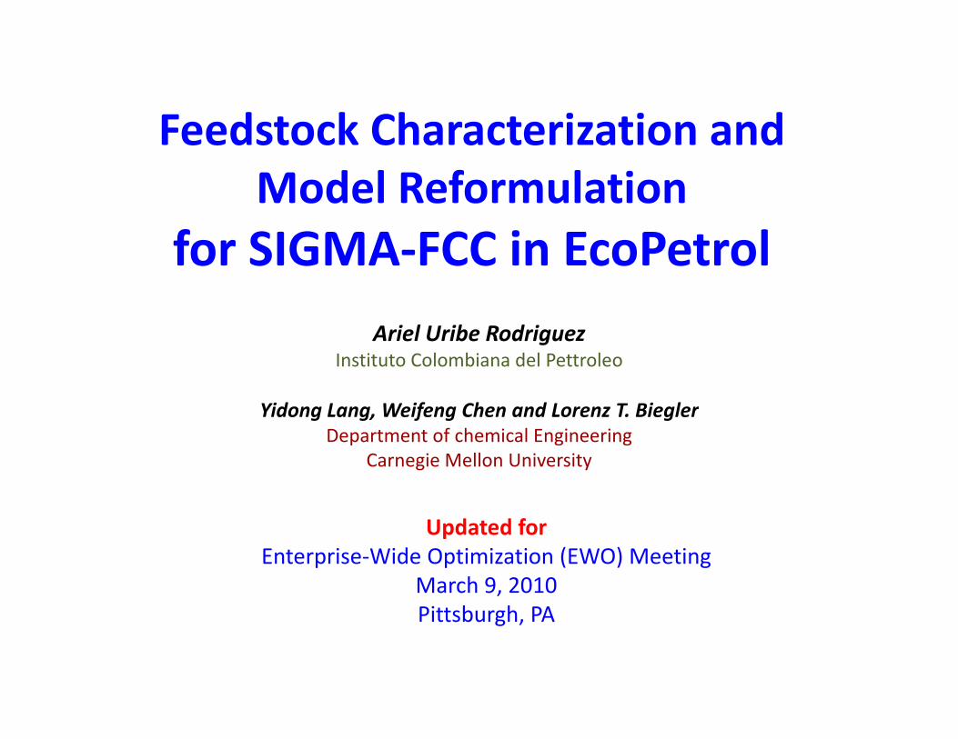
Feedstock Planning for FCCFeedstock Planning for FCC
Optimizing
Maximizing Yields
orFeed Allocation
TpreheatT
4
ProfitTreaction
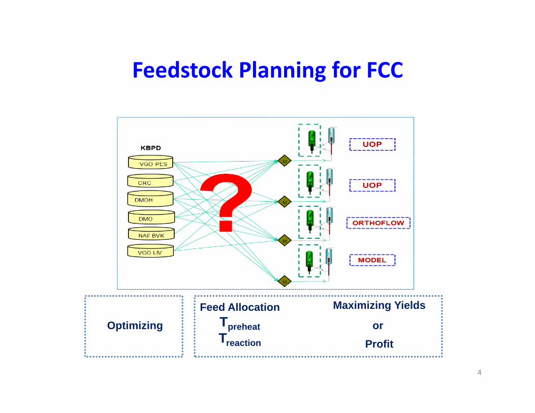
SIGMA‐FCC Planning Model Operational Constraints
Feed availability.
Limited feed to each UnitLimited feed to each Unit.
Minimum and Maximum capacity for each unit.
Routing. g
Minimum and Maximum riser and Preheat Temperatures.
Feed Q alit ConstraintsFeed Quality Constraints
Sulphur LimitConradson Carbon Limit
Coke Constraints
Coke Burnt and ProducedEmpirical and Semi-empirical Equations.The optimizer uses a mixed integer non‐linear model (MINLP).Solved with SBB (GAMS).
5
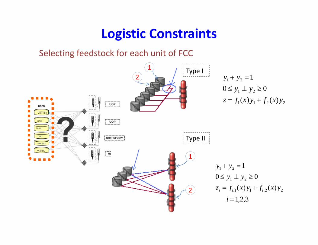
Logistic Constraints
1yy
Selecting feedstock for each unit of FCC1
2Type I
2211
21
21
)()(00
1
yxfyxfzyy
yy
2
Type II
121 yy1
Type II
321)()(
00
22,11,
21
21
iyxfyxfz
yyyy
iii23,2,1i

FCC Planning Model1. Correlations for Feedstock Properties
2. Stoichiometric Balances:
MODEL STATISTICS
BLOCKS OF EQUATIONS 110Regenerator
3. Heat balance:Regenerator- Riser
BLOCKS OF EQUATIONS 110 SINGLE EQUATIONS 525BLOCKS OF VARIABLES 73 SINGLE VARIABLES 371
GENERATION TIME
4. Parameter Tuning to reproduce Riser Plant Information GRB
MINLPSolved with SBB
(GAMS)
GENERATION TIME = 0.032 SECONDS 4 Mb
EXECUTION TIME =
5. Semi-empirical Equations: Reaction chemistry kinetics in the Riser
(GAMS)0.078 SECONDS 4 Mb
RESOURCE USAGE, LIMIT 0 691 1000 000
6. Empirical Equations:Product yields
7. Correlations for
0.691 1000.000
ITERATION COUNT, LIMIT 417 100000
Product Properties
7
Project Definition
1. Reformulate models from MINLP into NLP2. Reformulate models to improve their mathematical properties3. Introduce new developed technologies to solve NLP with better
performances (e.g. Ipopt with PAT)
Challenges• Models are blind for CMU because they are EcoPetrol proprietary• High nonlinearity ‐‐‐ Complicated empirical correlations in the models• Discontinuity ‐‐‐ Segmented correlations in the models• Complementarity ‐‐‐ Logistic constraints in the modelsComplementarity Logistic constraints in the models
8
Outlines of project designOutlines of project design
R f l t th l i bl N li• Reformulate the planning problems as Nonlinear programming (NLP) problems
• Reformulate the models with common techniques such as nonlinear reduction, variable scaling,…
• Reformulated the models with the techniques developed here, e.g. MPCChere, e.g. MPCC
• Try to use novel NLP solver such as Ipopt, therefore, for more convenience, translate the models from GAMS into AMPLAMPL
• Using parameter adaptive tuning (PAT) for Ipopt to solve the problems
Activities through EWO programg p g• Preliminary contact, Professors Biegler and Grossmann visit EcoPetrol, give
seminars, get basic information and relative materials.Ki k ff d f ll i di i i Pitt b h d i 2010 EWO ti• Kick‐off and following discussions in Pittsburgh during 2010 EWO meeting (March). The report 1 from EcoPetrol was presented to CMU, the CMU submitted a set of suggestions to the partner.
• on April 26, 2010, CMU got the Report 2 from EcoPetrolp , , g p• On July 26, 2010, CMU got the report 3 from EcoPetrol with a paper outlines led
by this project• On Aug. 12, 2010, CMU sent EcoPetrol the comments and suggestions on the
report 3report 3. • On Sept. 28, 2010, A presentation of the project is given in EWO meeting• At AIChE 2010 annual meeting, Larry and Ariel have a discussion.• On Nov. 26, 2010. A report of performances of Ipopt with two Planning models
in AMPL is sent to CMU from EcoPetrol.• CMU solves the two models successfully with Ipopt using PAT (Parameter
Adaptive Tunning) technique and the results sent to EcoPetrol.• On January 14 2011 CMU got workplan for 2011 from EcoPetrol• On January 14, 2011, CMU got workplan for 2011 from EcoPetrol
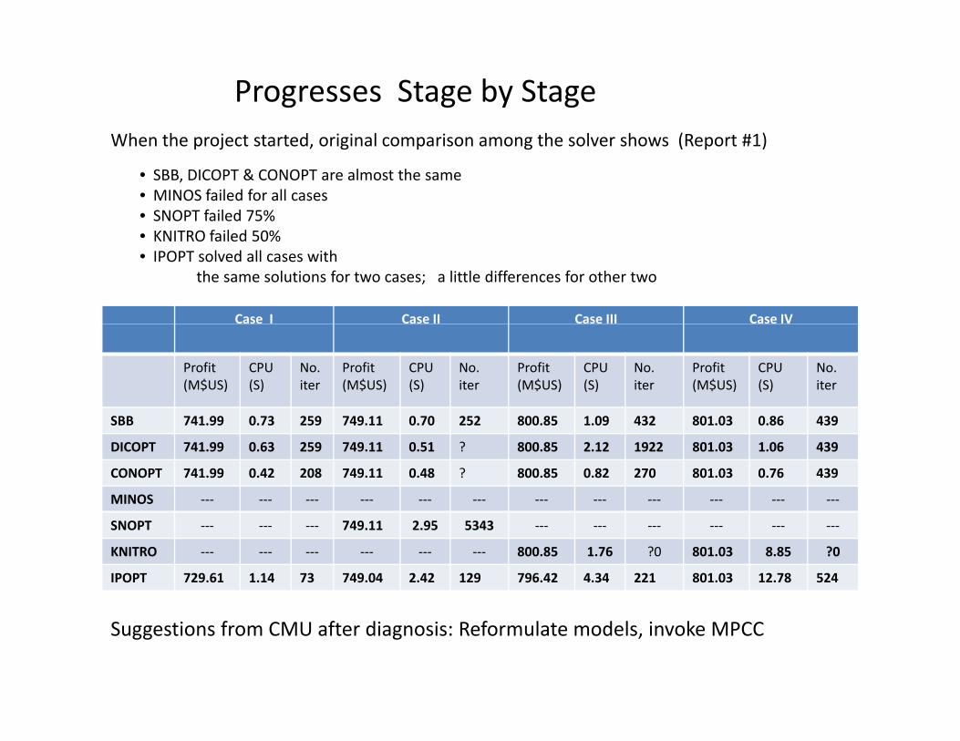
Progresses Stage by StageWhen the project started original comparison among the sol er sho s (Report #1)When the project started, original comparison among the solver shows (Report #1)
• SBB, DICOPT & CONOPT are almost the same• MINOS failed for all cases• SNOPT failed 75%
O f il d 0%
Case I Case II Case III Case IV
• KNITRO failed 50%• IPOPT solved all cases with
the same solutions for two cases; a little differences for other two
Profit(M$US)
CPU(S)
No.iter
Profit(M$US)
CPU(S)
No.iter
Profit(M$US)
CPU(S)
No.iter
Profit(M$US)
CPU(S)
No.iter
SBB 741 99 0 73 259 749 11 0 70 252 800 85 1 09 432 801 03 0 86 439SBB 741.99 0.73 259 749.11 0.70 252 800.85 1.09 432 801.03 0.86 439
DICOPT 741.99 0.63 259 749.11 0.51 ? 800.85 2.12 1922 801.03 1.06 439
CONOPT 741.99 0.42 208 749.11 0.48 ? 800.85 0.82 270 801.03 0.76 439
MINOS ‐‐‐ ‐‐‐ ‐‐‐ ‐‐‐ ‐‐‐ ‐‐‐ ‐‐‐ ‐‐‐ ‐‐‐ ‐‐‐ ‐‐‐ ‐‐‐
SNOPT ‐‐‐ ‐‐‐ ‐‐‐ 749.11 2.95 5343 ‐‐‐ ‐‐‐ ‐‐‐ ‐‐‐ ‐‐‐ ‐‐‐
KNITRO ‐‐‐ ‐‐‐ ‐‐‐ ‐‐‐ ‐‐‐ ‐‐‐ 800.85 1.76 ?0 801.03 8.85 ?0
IPOPT 729.61 1.14 73 749.04 2.42 129 796.42 4.34 221 801.03 12.78 524
Suggestions from CMU after diagnosis: Reformulate models, invoke MPCC
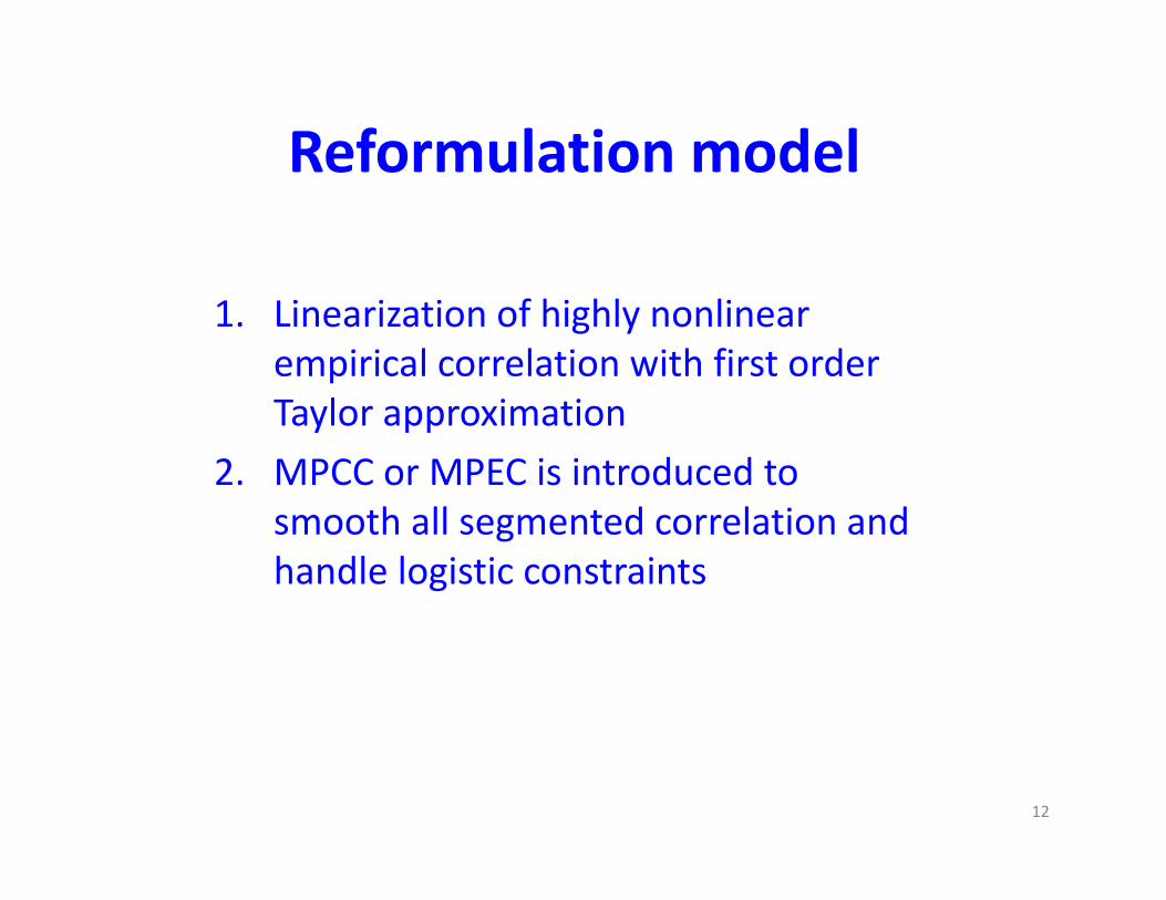
Reformulation modelReformulation model
1. Linearization of highly nonlinear empirical correlation with first order Taylor approximation
2. MPCC or MPEC is introduced to h ll d l dsmooth all segmented correlation and
handle logistic constraints
12
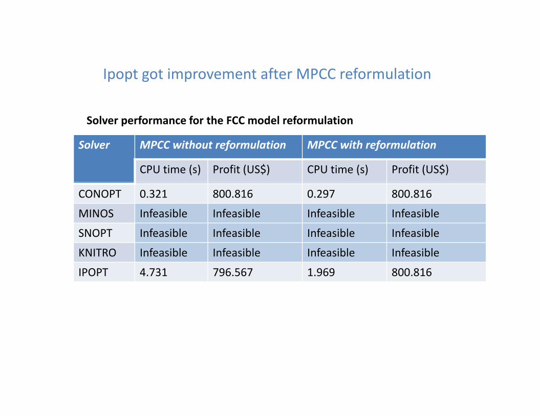
Ipopt got improvement after MPCC reformulation
Solver performance for the FCC model reformulation
Ipopt got improvement after MPCC reformulation
Solver MPCC without reformulation MPCC with reformulation
CPU time (s) Profit (US$) CPU time (s) Profit (US$)
CONOPT 0.321 800.816 0.297 800.816
MINOS Infeasible Infeasible Infeasible Infeasible
SNOPT Infeasible Infeasible Infeasible InfeasibleSNOPT Infeasible Infeasible Infeasible Infeasible
KNITRO Infeasible Infeasible Infeasible Infeasible
IPOPT 4.731 796.567 1.969 800.816
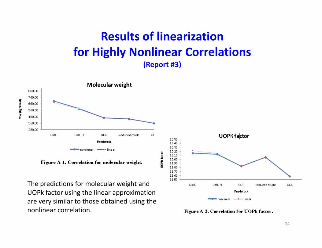
Results of linearization for Highly Nonlinear Correlations
(Report #3)
The predictions for molecular weight and UOPk factor using the linear approximation are very similar to those obtained using theare very similar to those obtained using the nonlinear correlation.
14
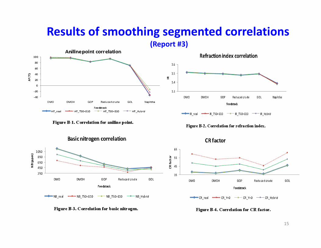
Results of smoothing segmented correlations(Report #3)(Report #3)
15
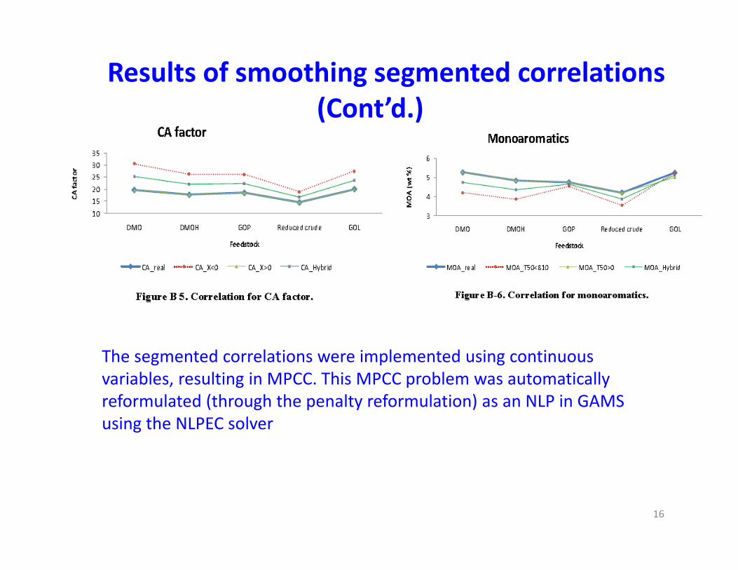
Results of smoothing segmented correlations(Cont’d )(Cont’d.)
The segmented correlations were implemented using continuous variables, resulting in MPCC. This MPCC problem was automatically reformulated (through the penalty reformulation) as an NLP in GAMS using the NLPEC solver
16
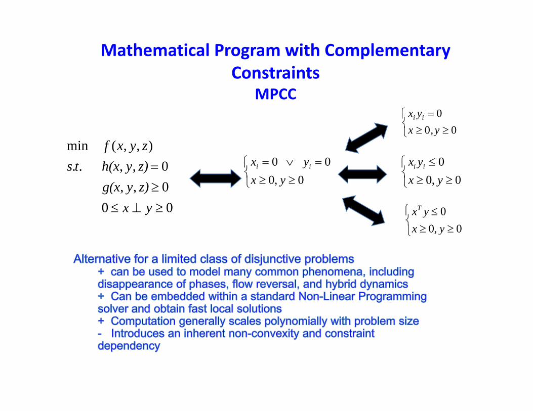
Mathematical Program with Complementary ConstraintsConstraints
MPCC
000yx ii
0,,..),,(minz)yh(xts
zyxf
000 0
yxyx ii
000yx
yx ii
00 y,x
000,,
yxz)yg(x 0,0 yx
0,00yx
yxT
0,0 yx
0,0 yx
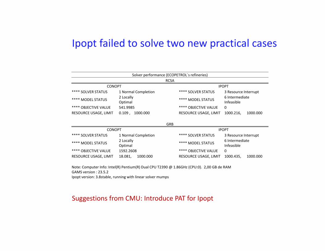
Ipopt failed to solve two new practical cases
Solver performance (ECOPETROL´s refineries)
Ipopt failed to solve two new practical cases
RCSACONOPT IPOPT
**** SOLVER STATUS 1 Normal Completion **** SOLVER STATUS 3 Resource Interrupt
**** MODEL STATUS 2 Locally Optimal **** MODEL STATUS 6 Intermediate
Infeasible **** OBJECTIVE VALUE 541.9985 **** OBJECTIVE VALUE 0RESOURCE USAGE, LIMIT 0.109 , 1000.000 RESOURCE USAGE, LIMIT 1000.216, 1000.000
GRBCONOPT IPOPT
**** SOLVER STATUS 1 Normal Completion **** SOLVER STATUS 3 Resource Interrupt 2 Locally 6 Intermediate**** MODEL STATUS 2 Locally Optimal **** MODEL STATUS 6 Intermediate
Infeasible **** OBJECTIVE VALUE 1592.2608 **** OBJECTIVE VALUE 0RESOURCE USAGE, LIMIT 18.081, 1000.000 RESOURCE USAGE, LIMIT 1000.435, 1000.000
Note: Computer Info: Intel(R) Pentium(R) Dual CPU T2390 @ 1.86GHz (CPU:0). 2,00 GB de RAMGAMS version : 23.5.2GAMS version : 23.5.2Ipopt version: 3.8stable, running with linear solver mumps
Suggestions from CMU: Introduce PAT for Ipopt
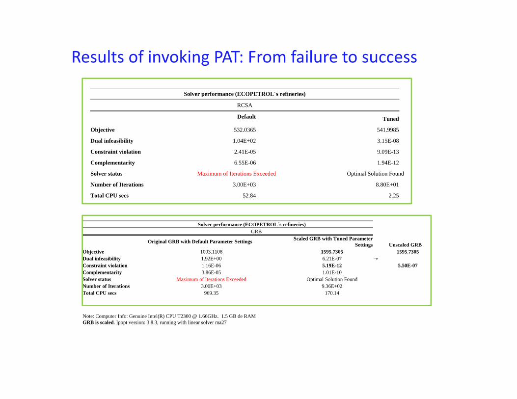
Results of invoking PAT: From failure to success
Solver performance (ECOPETROL´s refineries)
RCSA
Default Tuned
Objective 532.0365 541.9985
Dual infeasibility 1.04E+02 3.15E-08
Constraint violation 2.41E-05 9.09E-13
Complementarity 6.55E-06 1.94E-12
Solver status Maximum of Iterations Exceeded Optimal Solution FoundSolver status Maximum of Iterations Exceeded Optimal Solution Found
Number of Iterations 3.00E+03 8.80E+01
Total CPU secs 52.84 2.25
Solver performance (ECOPETROL´s refineries)Solver performance (ECOPETROL s refineries)GRB
Original GRB with Default Parameter Settings Scaled GRB with Tuned Parameter Settings Unscaled GRB
Objective 1003.1108 1595.7305 1595.7305Dual infeasibility 1.92E+00 6.21E-07 →Constraint violation 1.16E-06 5.19E-12 5.50E-07Complementarity 3.86E-05 1.01E-10p ySolver status Maximum of Iterations Exceeded Optimal Solution FoundNumber of Iterations 3.00E+03 9.36E+02Total CPU secs 969.35 170.14
Note: Computer Info: Genuine Intel(R) CPU T2300 @ 1.66GHz. 1.5 GB de RAMGRB is scaled. Ipopt version: 3.8.3, running with linear solver ma27
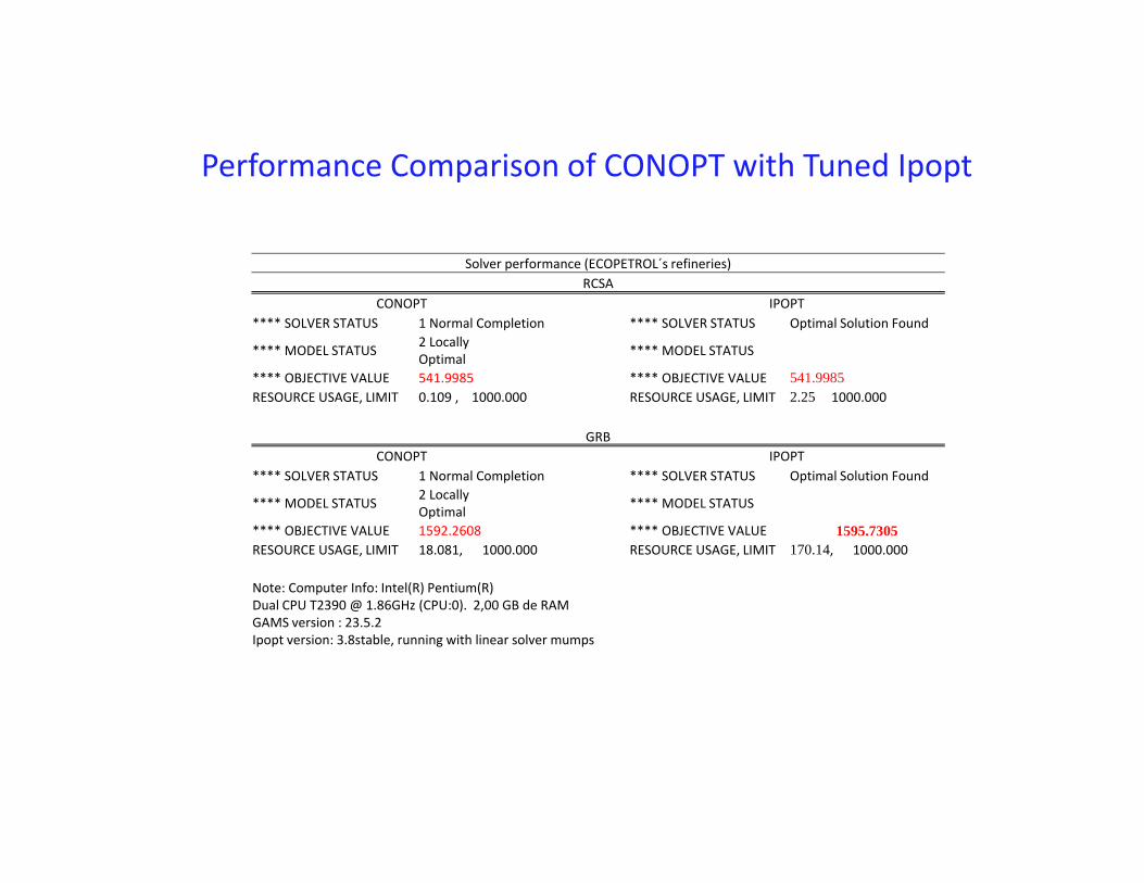
Performance Comparison of CONOPT with Tuned Ipopt
Solver performance (ECOPETROL´s refineries)
Performance Comparison of CONOPT with Tuned Ipopt
RCSACONOPT IPOPT
**** SOLVER STATUS 1 Normal Completion **** SOLVER STATUS Optimal Solution Found
**** MODEL STATUS 2 Locally Optimal **** MODEL STATUS
**** OBJECTIVE VALUE 541.9985 **** OBJECTIVE VALUE 541.9985RESOURCE USAGE, LIMIT 0.109 , 1000.000 RESOURCE USAGE, LIMIT 2.25 1000.000
GRBCONOPT IPOPT
**** SOLVER STATUS 1 Normal Completion **** SOLVER STATUS Optimal Solution Found2 Locally**** MODEL STATUS 2 Locally Optimal **** MODEL STATUS
**** OBJECTIVE VALUE 1592.2608 **** OBJECTIVE VALUE 1595.7305RESOURCE USAGE, LIMIT 18.081, 1000.000 RESOURCE USAGE, LIMIT 170.14, 1000.000
Note: Computer Info: Intel(R) Pentium(R) Dual CPU T2390 @ 1.86GHz (CPU:0). 2,00 GB de RAMDual CPU T2390 @ 1.86GHz (CPU:0). 2,00 GB de RAMGAMS version : 23.5.2Ipopt version: 3.8stable, running with linear solver mumps
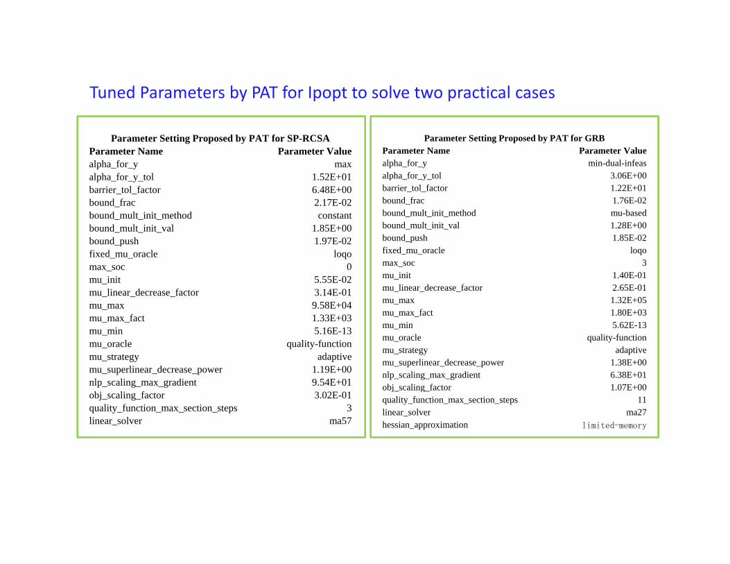
Tuned Parameters by PAT for Ipopt to solve two practical cases
Parameter Setting Proposed by PAT for SP-RCSAParameter Name Parameter Valuealpha_for_y maxalpha for tol 1 52E+01
Parameter Setting Proposed by PAT for GRBParameter Name Parameter Valuealpha_for_y min-dual-infeasalpha for y tol 3 06E+00alpha_for_y_tol 1.52E+01
barrier_tol_factor 6.48E+00bound_frac 2.17E-02bound_mult_init_method constantbound_mult_init_val 1.85E+00bound_push 1.97E-02
alpha_for_y_tol 3.06E+00barrier_tol_factor 1.22E+01bound_frac 1.76E-02bound_mult_init_method mu-basedbound_mult_init_val 1.28E+00bound_push 1.85E-02
fixed_mu_oracle loqomax_soc 0mu_init 5.55E-02mu_linear_decrease_factor 3.14E-01mu_max 9.58E+04mu max fact 1 33E+03
fixed_mu_oracle loqomax_soc 3mu_init 1.40E-01mu_linear_decrease_factor 2.65E-01mu_max 1.32E+05mu_max_fact 1.80E+03mu_max_fact 1.33E+03
mu_min 5.16E-13mu_oracle quality-functionmu_strategy adaptivemu_superlinear_decrease_power 1.19E+00nlp_scaling_max_gradient 9.54E+01
mu_min 5.62E-13mu_oracle quality-functionmu_strategy adaptivemu_superlinear_decrease_power 1.38E+00nlp_scaling_max_gradient 6.38E+01obj scaling factor 1 07E+00
obj_scaling_factor 3.02E-01quality_function_max_section_steps 3linear_solver ma57
obj_scaling_factor 1.07E+00quality_function_max_section_steps 11linear_solver ma27hessian_approximation limited-memory
Conclusions• Original FCC model developed in EcoPetrol contains logistic
constraints as well as highly nonlinear and segmented empirical correlations It is difficult to be used in planning toolempirical correlations. It is difficult to be used in planning tool SIGMA‐FCC.
• By introducing MPCC and reformulating the correlations and constraints of FCC, SIGMA‐FCC becomes efficient and effective to be used.
• By invoking PAT Ipopt becomes more robust• By invoking PAT, Ipopt becomes more robust• Preliminary results of optimal solutions show potential power
of SIGMA‐FCC in EcoPetrol• EWO is still helpful even for handling enterprise proprietary
2222