Yianni, Panayioti C. and Rama, Dovile and Neves, Luis C. and Andrews, John D. and Castlo, David (2016) A Petri-Net-based modelling approach to railway bridge asset management. Structure and Infrastructure Engineering, 13 (2). pp. 287-297. ISSN 1744-8980

Access from the University of Nottingham repository: http://eprints.nottingham.ac.uk/32046/1/A%20Petri-Net-based%20modelling%20approach%20to%20railway%20bridge%20asset%20managment.pdf

Copyright and reuse:

The Nottingham ePrints service makes this work by researchers of the University of Nottingham available open access under the following conditions.

This article is made available under the University of Nottingham End User licence and may be reused according to the conditions of the licence. For more details see: http://eprints.nottingham.ac.uk/end_user_agreement.pdf

A note on versions:

The version presented here may differ from the published version or from the version of record. If you wish to cite this item you are advised to consult the publisher’s version. Please see the repository url above for details on accessing the published version and note that access may require a subscription.

For more information, please contact eprints@nottingham.ac.uk

This is an Accepted Manuscript of an article published by Taylor & Francis in Structure andInfrastructure Engineering on 18/04/2016, available online: http://www.tandfonline.com/doi/full/10.1080/15732479.2016.1157826.

To cite this article: Panayioti C. Yianni, Dovile Rama, Luis C. Neves, John D. Andrews &David Castlo (2016): A Petri-Net-based modelling approach to railway bridge asset man-agement, Structure and Infrastructure Engineering, DOI: 10.1080/15732479.2016.1157826

A Petri-Net-based Modelling Approach to Railway Bridge Asset Management

Panayioti C. Yianni1, Dovile Rama1, Luis C. Neves1, John D. AndrewsI1, David Castlo2

Abstract

Management of a large portfolio of infrastructure assets is a complex and demanding task for transport agencies. Althoughextensive research has been conducted on probabilistic models for asset management, in particular bridges, focus has beenalmost exclusively on deterioration modelling. The model being presented in this study tries to reunite a disjointed systemby combining deterioration, inspection and maintenance models. A Petri-Net (PN) modelling approach is employed andthe resulting model consists of a number of different modules each with its own source of data, calibration methodologyand functionality. The modules interconnect providing a robust framework. The interaction between the modules canbe used to provide meaningful outputs useful to railway bridge portfolio managers.

Keywords: Rail, Bridges, Asset Management, Maintainability, Whole Life Cycle Costing, Petri-Net

1. Introduction

Railway structures are integral to the efficient runningof the transport network. Railways are used for both in-dustry and commuters so their use is critical from a socialand economic perspective. Trains can carry very heavyloads and the schedules mean that the frequency of trainsis relentless on supporting structures. With the futureintroduction of moving block signalling systems the fre-quency of trains will only increase which means the stresson civil structures will increase too.

A significant challenge is to be able to predict struc-tural deterioration. There are already industry guidelines(Network Rail, 2012) on the thresholds to inspect struc-tures and maintain structures, but there is limited under-standing of how structural defects evolve over time. Dif-ferent elements will deteriorate in different ways and sogrouping the elements helps to assign a deterioration pro-file to those elements. Additionally, some defects are moreor less likely to lead to other defects and knowing whichdefect an element suffers from and then monitoring thedefects development gives a great insight into predictingstructural deterioration.

There are three main material types used for railwaybridges: masonry, metallic and concrete. This study usesconcrete main girders as its exemplar element because con-crete bridges are becoming increasingly more popular andthe main girders are the elements that experience most

ICorresponding author: John D. Andrews; Email:John.An-drews@Nottingham.ac.uk

1Centre for Risk and Reliability Engineering, University of Not-tingham, Faculty of Engineering, University Park, Nottingham, NG72RD, United Kingdom.

2Network Rail, The Quadrant:MK, Elder Gate, Milton KeynesCentral, Buckinghamshire, MK9 1EN, United Kingdom.

structural loading and are critical to bridge safety. How-ever, the techniques and methods used in this study canbe applied to all railway bridges.

2. Stochastic Models

2.1. Markov Based Models

A number of different modelling approaches have beenused for bridge asset management, but the most populartype is stochastic modelling. Frangopol et al. (2004) makesit clear that stochastic models are superior to other mod-elling techniques for structural deterioration. Stochasticmodels use random variables and probability distributionsto predict the deterioration over time. Frangopol et al.(2004) states that it would be better to model deterio-ration in terms of a time-dependent stochastic process.Morcous et al. (2010) reports from Ditlevsen (1984) thatstructural deterioration is a complex process and thereis a considerable amount of uncertainty in the structures“micro-response” which means that stochastic models of-fer practicality and reliability.

Markov based models have been used for bridge dete-rioration for 25 years. Jiang and Sinha (1989) were oneof the first to study bridge deterioration with a Markovbased model. They used a population of 5,700 bridges inIndiana, USA, from which 50 were randomly selected assamples. The paper discusses the methodology of gener-ating the transitional probability based on condition scoredata of bridges of different ages. The bridge conditionswere scored by guidelines set out by the Federal HighwayAdministration (FHWA), 0-9 with 9 being the rating ofa new bridge. They noticed that as the bridge ages thedeterioration rate also changes. The paper follows on tosay that Markov based approaches would be useful in thisstochastic situation. The paper has been widely cited as

Preprint submitted to Structure and Infrastructure Engineering April 19, 2016

pioneering the technique, however there was no applicationon bridge condition data.

Cesare et al. (1992) developed the technique further byincorporating a repair policy into the model. The studyused 850 bridges in New York state totalling over 2,000spans. The Markov chain model was designed with 7 statesranging from 1, potentially hazardous, to 7, new condition.Their approach splits the asset into major components e.g.superstructure, deck and piers. The model assumes thatdeterioration of each element is independent of all otherbridge elements. The repair policy is implemented with arepair matrix that improves the condition by either 10% or20% of the bridge condition scores in condition state 3 orless. There is little clarification about the repair policiesbut the authors claim to be able to predict the evolutionof the average condition state of a set of bridges and thecondition for a specific bridge. This approach was usedby the Association of State Highway and TransportationOfficials (AASHTO) to create Pontis which serves as themost widespread Bridge Management System (BMS). Itis used to manage over 500,000 bridges in 45 US states(Sobanjo and Thompson, 2011).

Scherer and Glagola (1994) attempted to apply theMarkov approach to real-world data from 13,000 bridges inVirginia. The paper uses the same 7 states used in Cesareet al. (1992). However the author uses the condition of thewhole bridge rather than bridge components. The authorthen comments that the Markov chain approach createsSn states where S is the number of states and n is thenumber of assets in the study. This would have created713,000 states which contemporary computers would havestruggled to simulate. To tackle this issue the author cre-ates a number of classes based on: road system, climate,traffic loading, bridge spans, bridge age and bridge type.The total number of classes is 216 and a typical bridge ex-ample was chosen for each class. This reduces the numberof states to 7216. The paper tried to address the issue withMarkov state inflation (Sn) by grouping the bridges andthen selecting typical examples from each group. The pa-per does identify the issue of a bridge that moves betweengroups over its lifetime due to deterioration.

Morcous (2006) studied the Quebec transport bridges,totalling 9,678 structures, including bridges of differenttypes and culverts. Overall the data included 500,924 el-ement inspections from 1997 to 2000. The performanceindicator ranged from 0-100 with a higher number indi-cating a better condition. All inspection changes that in-dicated an increase in condition were striped out to elimi-nate the effects of maintenance or inspector variance. Thepaper lays out some assumptions: firstly, bridge inspec-tions are assumed to be carried out at a pre-determinedfixed interval. Secondly, future bridge condition dependsonly on present condition, ignoring historical conditions,highlighting the “memoryless” Markov property. Morcous(2006) states that these assumptions affect the reliabilityof the predictions and that the assumptions were designedto reduce the computational complexity and streamline

the decision-making operation. The paper analyses theinspection interval to compute a normally-distributed in-spection interval with a mean just over 2 years. The papercalculated the Transition Probability Matrix (TPM) usingthe frequency approach. This paper incorporates a differ-ent approach using Bayes’ rule which is used to adjust theTPM for the variance in inspection frequency. This is thencompared to the before and after effects of Bayes’ rule. Thepaper closes with a figure of 22% for the improvement pos-sible in estimating the service life of the bridge decks (themost critical component) with the inclusion of Bayes’ rulein the adjustment of the TPM.

The models that have been discussed are Markov basedmodels. Markov models form the basis for the predictionmodule found in many BMS systems. They have had un-paralleled adoption in the field of infrastructure facilities.Morcous (2006) makes it clear that the Markov approachis the most commonly used of all the stochastic modelsfor predicting performance in bridges, highways, sewerageand water distribution. That is not to say that Markovmodels are without limitation. Additionally, some of thetechniques used to simplify Markov model computationare not directly Markovian limitations, but are limitationsto using the Markov approach in structural deteriorationmodelling. Some of those limitations include:

• Markov chain based models assume that time inter-vals are discrete intervals, the bridge population isfixed and the TPM probabilities are static which canbe inaccurate (Morcous et al., 2002).

• Transition probabilities in the TPM are difficult toaccurately calculate and can often require manipu-lation by expert judgement (Frangopol et al., 2004).

• Often inspection data where the condition has in-creased is disregarded due to difficulty in reliablyascertaining which assets were repaired and what re-pair action was applied (Robelin and Madanat, 2007;Morcous et al., 2002).

• The condition states are defined as discrete statesbut often there will be borderline candidates andcritical elements which require expert judgement forcorrect classification, which can be subjective. Fran-gopol et al. (2004) argues that a more detailed, con-tinuous, measurement criterion would be superior.

• The Markov modelling approach suffers from a rapidexpansion of states when interactions between ele-ments are considered. The number of model statesfollows Sn where S is the number of states and n isthe number of elements. Even though this is oftennot a problem for modern bridge management sys-tems, it is still a limitation of the technique (BritishStandards Institution, 2012).

2

2.2. Petri-Net Based Models

PNs were developed by Petri (1962). They have had in-creasing application in transportation, manufacturing andbusiness for modelling dynamic, distributed systems (BritishStandards Institution, 2012). PNs are not as commonas other conventional modelling techniques and being themain method employed in this work, they are describedin detail in Section 3. Recent work demonstrated thatPNs are appropriate for deterioration modelling (Andrews,2013). The approach used four states to describe the as-set deterioration process: new, degraded needing mainte-nance, degraded needing speed restrictions and degradedneeding line closure. The model was designed for track de-terioration rather than structural deterioration, howeverthe author mentions that the PN modelling technique hasa great deal of flexibility and the PN model presented inthe paper is significantly more developed than others foundin literature.

Rama and Andrews (2013b) used a number of simplePN subnets to model the railway infrastructure in a hier-archical, modular structure. A number of different sub-netmodules were created for component deterioration, main-tenance, inspection and renewal. A modelling frameworkwas presented where the hierarchy was laid out. At the toplevel the whole railway is subjected to track, rail and geom-etry inspections. Then, at the lower levels, depending onthat particular 1/8th of a mile section, sleepers, fasteningsand ballast are modelled. Each of the sub-nets connectsto one another and a resource allocation PN is created tomanage occupied maintenance staff. For each section oftrack, the appropriate sub-net modules are amalgamated.The paper mentions that having a library of PNs specificto individual assets could be beneficial to generating a de-tailed, realistic model of the whole system.

Le and Andrews (2014b,a) created a bridge model us-ing a PN approach. A number of PN sub-nets were gen-erated for the components that make up the bridge (e.g.deck, girders and abutments). Each component was de-tailed with deterioration, inspection and maintenance pro-cesses. For each bridge asset the elements are consideredand the corresponding sub-PNs chosen to create a com-plete bridge model. The state descriptions in this modelwere not related to deterioration, but the maintenanceaction required for rehabilitation, similar to Yang et al.(2009). This model uses Coloured Petri-Nets (CPNs) totrack different individual bridge elements within the samesub-net. The advantage of CPNs here is that coloured to-kens within a sub-net could hold tuple information. Thiscan be used in analysis, for example, the number of mainte-nance occurrences before element replacement. The modelinputs are deterioration characteristics for different bridgecomponents and the maintenance/renewal strategy param-eters. The author uses Monte Carlo sampling for all stochas-tic transitions. A simulation duration of 60 years was usedand the results converged after roughly 200 simulations;this took under 10 minutes to perform.

Overall, there is a strong case that structural deterio-ration is a stochastic process and therefore a probabilisticmethod is preferred. Due to numerous Markov limitations,explained in section 2.1, there is a suitable draw to usingPNs to model structural deterioration.

3. Petri-Nets

PNs are directed bipartite graphs. A bipartite graphis valid if its vertices can be grouped into two subsets Uand V . Each arc connects a vertex from subset U to a ver-tex in subset V . They are built with two types of nodes:places and transitions. In bridge modelling, places are rep-resentative of element condition (e.g. as new, good, poor).Tokens are arguably the most important feature of a PNmodel. A token, representing a bridge or element, occu-pies a place. Through this, the condition of the element isdefined at any given time. I.e. a token in a place markedas new” means that a particular bridge element is in an asnew” condition. Transitions are used to move tokens fromplace to place mimicking deterioration, for instance. Thearcs are graphical representations of relationships betweenplaces and transitions. No two places or transitions canbe directly connected with an arc (Reisig, 2013). Thesecomponents can be seen in Figure 1.

Place Place with token Arc Transition

Good Condition Poor Condition

t

Figure 1: Components of a Petri-Net with a simple example.

3.1. Coloured Petri-Nets

CPNs are an extension to simple PNs previously dis-cussed. They were developed by Jensen (1997) as theamalgamation of simple PNs and programming languages.British Standards Institution (2004) discusses the advan-tage of CPNs as a way of avoiding the exponential increasein number of states with the number of elements.

In simple PNs, the tokens are anonymous and indistin-guishable, their importance comes from their presence/ab-sence in the place. However with CPNs, there is an addi-tional constraint: transitions can only be activated if allthe input places have the correct number of tokens andthe tokens must match the transition criteria, known asthe “guard”. An example of this in bridge modelling maybe for minor interventions. After a certain amount of mi-nor interventions, a more major intervention may have tobe carried out. Therefore, a counter place may accumu-late tokens based on the number of minor interventions,when the threshold is reached, the transition fires to in-hibit further minor interventions. The phrase “coloured”

3

in CPNs does not necessarily mean that each token has itsown colour; but only tries to clarify that now tokens can beof different types with different data sets and characteris-tics. The data held within the token in known as the token“tuples”. The tuples within the token could be modifiedby the transition, for instance if one of the pieces of infor-mation in the token was the age of the asset, that numbercould increase within the tuple when the transition fires.

The transitions become more sophisticated in CPNs asthey do not simply consume and produce tokens at theallocated time, but they now perform functions on thedata within the token itself. This affords CPNs a greatdeal of flexibility beyond simple PNs. A basic exampleof a CPN can be seen in Figure 2. The transition hastwo input places, each containing a token. The transitionhas a guard to satisfy which is that the input tokens bothhave to have integers larger than one. The token in thetop place contains two pieces of information: an integernumber and a string. The token in the bottom place onlycontains an integer number. The integer is bound to wand the string to s. The guard is satisfied, so upon firing,the transition consumes the input tokens and generates atoken in the output place. This output token contains aninteger and a string. The integer is the product of the twoinput token integers. The string remains unmodified inthis example. The binding of the tuples, the satisfying ofthe transition and the subsequent modification of the tupleinformation is known as occurrence. This functionalityenables a huge variety of features to be incorporated intoPNs which affords it a high level of flexibility. More detailsabout advanced CPN functions are described in Le andAndrews (2014b).

int:4

int:2,string:“Metal”

w, v > 1

int:v

int:w,string:s

int:v · w,string:s

int:8,string:“Metal”

w, v > 1

int:v

int:w,string:s

int:v · w,string:s

Figure 2: Simple example of a CPN before the transition fires (a)and after the transition fires (b)

4. Deterioration, Inspection and Maintenance Poli-cies

4.1. Condition States

Network Rail (NR) inspect each Sub-Minor element ofeach bridge and give it a rating according to its condition.The condition of elements is determined during inspec-tion with a conditional matrix, which ranks the conditionbased on Severity Extent Rating (SevEx). Each time anelement is inspected, its condition is recorded. For con-crete bridges, the example used in this study, the SevExratings go from A1 (perfect condition) to G6 (permanentstructural damage). The first character refers to the typeof defect and the second refers to the extent of the defect,the full SevEx ratings can be seen in Table 1. The mostcommon defects seen in concrete elements are cracking andspalling, Nielsen et al. (2013) found them to be as high as89.9% of all concrete defects.

Table 1: SevEx defects for concrete structures (Network Rail, 2012)

Severity Defect DefinitionA No visible defectsB Surface damage, Minor spalling, Wetness,

Staining, Cracking <1mm wideC Spalling without evidence of corrosion,

Cracking ≥ 1mm wide without evidence ofcorrosion

D Spalling with evidence of corrosion, Cracking≥ 1mm wide with evidence of corrosion

E Secondary reinforcement exposedF Primary reinforcement exposedG Structural damage to element including per-

manent distortion

Extent Definition1 No visible defects2 Localised defect due to local circumstances.3 Affects <5% of the surface of the element.4 Affects 5%-10% of the surface of the element.5 Affects 10%-50% of the surface of the element.6 Affects >50% of the surface of the element.

4.2. Inspection Interval

The current NR policies lay out guidelines for wheninspection should be scheduled. NR uses two classes ofinspection. The first, detailed inspections, are performedwithin touching distance. Each of the elements are in-spected and the SevEx score recorded. The second, visualinspections, are carried out annually. An inspector usesthe last detailed inspection to make sure that no majorchanges to element condition have occurred. No scoringis carried out on visual inspections. Henceforth, any ref-erence to an inspection is referencing detailed inspections.Network Rail (2010b) describes how the condition of thestructure is then converted to a risk level and that cor-responds to an inspection interval. Rather than have to

4

convert from the condition state to a risk level to deter-mine the inspection interval, a back-calculation was doneso that the inspection interval could be directly related tothe condition state. This was then incorporated into themodel so that the inspection schedule could be determinedduring simulation.

Table 2 shows the SevEx states and their associatedinspection regime. The SevEx states of better conditionsare deemed to be lower risk and have a maximum inspec-tion interval of 12 years for concrete elements. The SevExstates of medium conditions are of a medium risk and arerecommended to be inspected no later than 6 year inter-vals. Finally, the worse SevEx states have a higher risk andmust be inspected no less frequently than every 3 years.

Table 2: Table showing the SevEx states and their correspondinginspection interval

Interval (years) States12 A1, B2-B5, C2-C3, D26 B6, C4-C6, D3-D5, E2-E5, F2-F33 D6, E6, F4-F6, G2-G6

4.3. Maintenance Actions

The current NR policies lay out guidelines for whenmaintenance should be scheduled. This is decided uponby an index number known as Bridge Condition MarkingIndex (BCMI). An A1 condition would relate to an BCMIof 100 and a G6 would relate to an BCMI of 0. The main-tenance thresholds in Network Rail (2010a) give the main-tenance thresholds in terms of BCMI. The fundamentalcondition that all elements must meet or exceed is knownas the “Basic Safety Limit” which varies for different ma-terials. To determine the correct maintenance action, theSevEx condition must be converted to the BCMI and thenchecked against the thresholds in Network Rail (2010a).To be able to determine the appropriate maintenance ac-tion in the PN model, the thresholds were back-calculated,through the BCMI to determine the SevEx conditions thatthey relate to. This was carried out so that the appropri-ate maintenance action could be determined during simu-lation.

Whilst exploring the database of inspections, it was ev-ident that there were repair works carried out above thecondition threshold for intervention. In discussions withthe NR Principal Engineers, it became clear that therewere two avenues for intervention: 1) the elements thathad breached the NR condition threshold and 2) the ele-ments that were above the threshold but the local mainte-nance team had decided they should intervene. Therefore,in essence, there are two types of intervention, Minor andMajor intervention. In Table 3 the SevEx state thresholdsfor different maintenance actions are represented. Thereis a great deal of similarity between the thresholds seen inTables 2 and 3 which suggests the same set of principleswere employed by NR policy makers.

Table 3: Table showing the SevEx state thresholds for different main-tenance actions.MaintenanceAction

States

Minor Repair B2-B4, C2-C3, D2Major Repair B5-B6, C4-C6, D3-D5, E2-E4, F2-F3Replacement D6, E5-E6, F4-F6, G2-G6

5. Data Source

The data used for this study was amalgamated from anumber of different datasets. The Civil Asset Register andReporting System (CARRS), Structure Condition Mon-itoring Index (SCMI), Cost Analysis Framework (CAF)and MONITOR databases were used, provided by NR.CARRS contains general asset information e.g. the loca-tion of the bridge, the material category, territorial clas-sification, etc. The SCMI database contains informationregarding the condition of the structure following an in-spection. CAF and MONITOR contain work items splitbetween smaller jobs and larger interventions, these wereused to determine scheduling and work times as well ascosts. Snapshots of the databases were provided coveringdifferent time periods so the databases had to be com-bined and cleaned to ensure that duplicates were removedas well as erroneous data entries. The combined databasecontains inspections between 1998 and 2014. In total therewere records of inspection of 25,949 bridges. Each bridgecomprises a number of major elements; the number of ma-jor elements which were inspected totalled 273,427. Eachof the major elements can be broken down into minorelements; minor elements which were inspected totalled563,150. The number of inspections on minor elementstotalled 1,397,748.

The exemplar element in this study is concrete maingirders. There are 4,434 concrete bridges recorded in thepopulation and the main girders are one of the most crit-ical minor elements. The number of repeat inspectionson concrete main girders totalled 407,708. This was usedto calibrate various model parameters including structuraldeterioration.

To be able to understand how structural deteriorationevolves, one inspection is not enough as a change in con-dition is required. The vast majority of elements (82.68%)have only had two inspections. The percentage of elementswith three inspections is 15.83%. The number of elementsthat have had 4-6 inspections is 1.49%. The databaseranges roughly 16 years and most elements are inspectedevery 6 years so 2 inspections per element would be ex-pected. The elements that are in the range of 4-6 inspec-tions usually have an inherent asset defect (e.g. structuralsubsidence) that causes a number of issues to occur hencethe increase in inspections. Overall however, there is alarge portfolio of structures to inspect so the number ofelements with multiple inspections grows continuously.

5

6. Petri-Net Model

The model which has been developed uses a bottom-upapproach rather than a top-down approach. To that effect,the model is asset and sub-asset level rather than at thenetwork level. The model represents an asset with thePN tokens representing elements of the asset. To modela complete bridge, each element of the bridge would berepresented by a token in the model. The model is pri-marily condition based as this is currently the main driverof the decision making processes since it is often the onlyavailable information for large bridge stocks. The limita-tion of this approach has been described, amongst others,by Neves and Frangopol (2005). The capability to modelinteractions between elements has been incorporated intothe model, however has not been used in this study. Forexample, element interaction could occur during mainte-nance; one girder that requires replacement may lead toanother that is in a moderate condition being repairedtoo. In this study, elements are considered individually asoppose to groups of elements with interactions. Finally,this model can be used to optimise maintenance and in-spection strategies using a multitude of algorithms includ-ing Genetic Algorithms (GAs) (Elbehairy et al., 2006),Dynamic Programming (Sniedovich, 2010) and ParticleSwarm (Yang et al., 2012) although not considered in thisstudy.

The PN bridge model uses a number of CPN features,but is referred to as a PN model for simplicity. The CPNfeatures are used in two ways: 1) each token contains tupleinformation about the element i.e. each token representsan element of the bridge and contains all the relevant in-formation about that element within the token e.g elementtype, material and location 2) there are advanced transi-tion functions built into the model which can aid in mod-elling complex decision-making processes without makingthe resulting model unduly complex e.g: probabilistic out-comes, condition dependant delays and condition trans-posing.

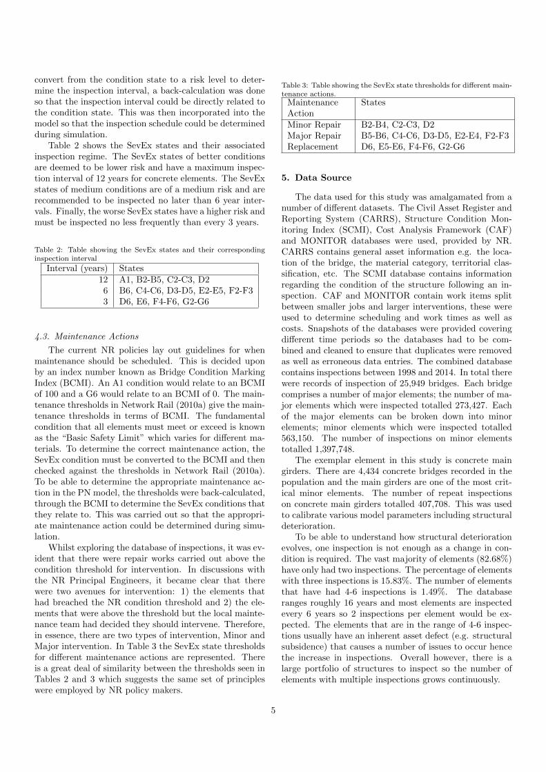
The PN bridge model comprises of a number of “mod-ules”. Each module has a different purpose e.g. elementdeterioration, inspection, maintenance, etc. They vary intheir formation and modelling approach and so each mod-ule is explained individually. Figure 3 describes the generaloverview of the modules and how they interact.

Figure 4 gives an example of how the modules interactto form the bridge model framework. Consider a bridge el-ement with a deterministic starting condition of A1. Thiscondition, according to current policy, requires an inspec-tion every 12 years (see Table 2). Transition times are gen-erated, based on historic data, for the possible movement(i.e. to condition states B2, B3 and C2). The transitionwith the probabilistically defined shortest time is selected.This transition fires at t = 5 which moves the system statefrom t1 to t2. At this point, the transition times are gen-erated for the possible movement to condition states (B3,C2 and C3). Again, the shortest transition time is chosen

Deterioration Module:Contains the element de-terioration profiles.

Inspection Module: Dy-namically adapts theintervention regime de-pending on the deteriora-tion level.

Intervention Module:Performs the work re-quired for the deteriora-tion level and the con-dition improves accord-ingly.

Figure 3: A general overview of the PN model and its componentmodules. Each of the modules performs a different function andinteracts with the other modules as shown.

and the element deteriorates to condition B3 at t = 10.Transition times are generated for the possible movementto condition states (B4, C3 and C4). However, at t = 12,the scheduled inspection takes place. This reveals the con-dition of the element to the bridge managers. According tocurrent policy, an element in condition B3 would be eligi-ble for a Minor Intervention (see Table 3). The inspectiontakes place at t = 12, however there is an associated de-lay to carry out the intervention whilst bridge possessionsare scheduled and materials ordered. The intervention iscarried out at t = 13 which, in this example, improves thecondition of the element to the A1 condition. Althoughnot implemented in this study, the model includes the ca-pability of introducing a number of different condition im-provement profiles. Another inspection is scheduled in afurther 12 years. The deterioration starts again with thetransition times from condition A1 to condition states B2,B3 and C2 generated.

6.1. Deterioration

6.1.1. Calibrating Deterioration

One way to format the historic data is to use a time-based approach (Agrawal et al., 2010; Niroshan et al.,2014; Rama and Andrews, 2013a), which is typically usedwith PNs. Each structure is routinely inspected and soa record can be built up of the health of each elementthat the structure comprises of. However, NR inspecttheir structures roughly every 6 years which is not regularenough to capture the data to use this approach. Thismeans that lifetime distributions cannot be obtained fromthe data. Due to this limitation, the movement betweencondition states of the structure is assumed to be of aconstant rate and is equivalent to a constant failure rate,

6

0 2 4 6 8 10 12 14 16 18 20B4

B3

B2

A1

Inspection

Intervention

t1 t2 t3 t4

Years

Con

dition(SevEx)

Figure 4: An example of a single bridge element. The effects ofthe deterioration, inspection and intervention modules are demon-strated.

λ. In this situation, failure is defined as moving from onecondition to another e.g. B2 to B3.

Most models that incorporate structural deteriorationuse a one dimensional condition state scale e.g. new, good,poor (Cesare et al., 1992; Morcous, 2006; Le and Andrews,2014a). However, structures fail by multiple failure modes,as seen in Table 1. Different defects deteriorate at differ-ent rates and are more or less likely to lead onto otherdefects. For this reason keeping the failure modes sepa-rate was an important part of the deterioration module.This study uses a 2-D condition scale comprising the de-fect type and the magnitude of the defect. Although thisapproach enhances the realism of the deterioration, it alsomakes calibration more difficult. However it was seen thatthe advantages gained from having condition states thatwere more true-to-life outweighed the problematic calibra-tion process.

There has also been a review of the time steps used inthe model. NR inspect their structures roughly every 6years, however for the model a more regular time step isrequired. Additionally, having a smaller time step shouldgive more transparency to the model as degradation canbe followed more closely. The following assumption hasbeen implemented: the condition of an element can onlymove to the immediately neighbouring states. To satisfythis assumption, a time step of one month was selectedas it was seen as the longest unit of time that would notenable an element to move beyond one condition state.Most bridge management models (Le and Andrews, 2013;Agrawal et al., 2010; Cesare et al., 1992) choose 1 yeartime steps, however this would not satisfy the constraintpreviously mentioned, in particular regarding duration ofmaintenance actions. Figure 5 shows the condition stateswith the movements that are possible between them.

In practice, the element condition movements have beencalculated from historic data. The assumption being usedis that the condition of an element can only move to the

A1

B2 B3 B4 B5 B6

C2 C3 C4 C5 C6

D2 D3 D4 D5 D6

E2 E3 E4 E5 E6

F2 F3 F4 F5 F6

G2 G3 G4 G5 G6

Figure 5: Condition states and their allowed progression; each ofthe states are connected to its neighbouring states, but only if itrepresents deterioration.

immediately neighbouring states because of the monthlytime interval. The Mean Time to Failure (MTTF) wasthen calculated for the positions being considered, usingthe following equation:

MTTFB2→B3 =t · nB2

mB2→B3(1)

where t is the time interval, in this case 72 months be-tween inspections, nB2 is the total number of elementsresiding in state B2 at the beginning of the time interval,and mB2→B3 is the number of elements that move fromB2 to B3. The MTTF is then used to calculate the failurerate:

λB2→B3 =1

MTTFB2→B3(2)

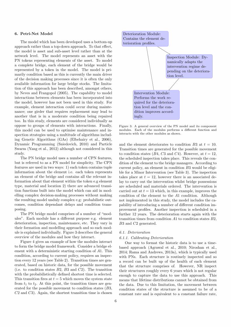
where λ is the failure rate. Here λB2→B3 represents therate of an element moving from state B2 to B3. Each tran-sition is embedded with its corresponding λ value whichis then used to generate the transition time in the PNdeterioration module from the exponential distribution.Historical data was used to obtain the occurrences be-tween each condition state e.g. the number of elementsthat move from condition B2 to condition B3. These werethen used to compute the MTTFs. The failure rates arethe reciprocal of the MTTFs which are embedded into thePN transitions so that the same deterioration profile canbe replicated in the model. Some of these values can beseen in Table 4.

The deterioration profile for concrete girders, the crit-ical element in this study, can be seen in Figure 6. Thisgraph shows the probability of being in different conditionsover time with no intervention. This is useful to be ableto see how defects evolve over time. The simulation wasdone with the element starting in a new (A1) condition.

7

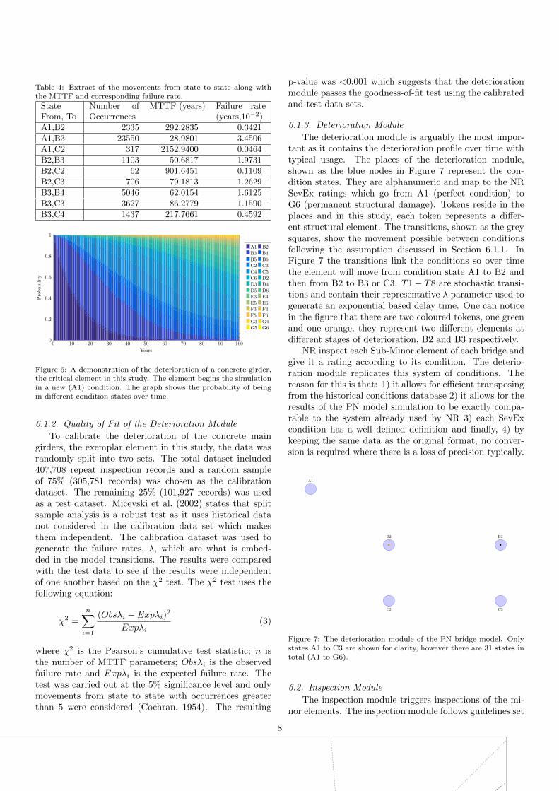
Table 4: Extract of the movements from state to state along withthe MTTF and corresponding failure rate.

StateFrom, To

Number ofOccurrences

MTTF (years) Failure rate(years,10−2)

A1,B2 2335 292.2835 0.3421A1,B3 23550 28.9801 3.4506A1,C2 317 2152.9400 0.0464B2,B3 1103 50.6817 1.9731B2,C2 62 901.6451 0.1109B2,C3 706 79.1813 1.2629B3,B4 5046 62.0154 1.6125B3,C3 3627 86.2779 1.1590B3,C4 1437 217.7661 0.4592

0 10 20 30 40 50 60 70 80 90 1000

0.2

0.4

0.6

0.8

1

Years

Probab

ility

A1 B2B3 B4B5 B6C2 C3C4 C5C6 D2D3 D4D5 D6E3 E4E5 E6F3 F4F5 F6G3 G4G5 G6

Figure 6: A demonstration of the deterioration of a concrete girder,the critical element in this study. The element begins the simulationin a new (A1) condition. The graph shows the probability of beingin different condition states over time.

6.1.2. Quality of Fit of the Deterioration Module

To calibrate the deterioration of the concrete maingirders, the exemplar element in this study, the data wasrandomly split into two sets. The total dataset included407,708 repeat inspection records and a random sampleof 75% (305,781 records) was chosen as the calibrationdataset. The remaining 25% (101,927 records) was usedas a test dataset. Micevski et al. (2002) states that splitsample analysis is a robust test as it uses historical datanot considered in the calibration data set which makesthem independent. The calibration dataset was used togenerate the failure rates, λ, which are what is embed-ded in the model transitions. The results were comparedwith the test data to see if the results were independentof one another based on the χ2 test. The χ2 test uses thefollowing equation:

χ2 =

n∑i=1

(Obsλi − Expλi)2

Expλi(3)

where χ2 is the Pearson’s cumulative test statistic; n isthe number of MTTF parameters; Obsλi is the observedfailure rate and Expλi is the expected failure rate. Thetest was carried out at the 5% significance level and onlymovements from state to state with occurrences greaterthan 5 were considered (Cochran, 1954). The resulting

p-value was <0.001 which suggests that the deteriorationmodule passes the goodness-of-fit test using the calibratedand test data sets.

6.1.3. Deterioration Module

The deterioration module is arguably the most impor-tant as it contains the deterioration profile over time withtypical usage. The places of the deterioration module,shown as the blue nodes in Figure 7 represent the con-dition states. They are alphanumeric and map to the NRSevEx ratings which go from A1 (perfect condition) toG6 (permanent structural damage). Tokens reside in theplaces and in this study, each token represents a differ-ent structural element. The transitions, shown as the greysquares, show the movement possible between conditionsfollowing the assumption discussed in Section 6.1.1. InFigure 7 the transitions link the conditions so over timethe element will move from condition state A1 to B2 andthen from B2 to B3 or C3. T1− T8 are stochastic transi-tions and contain their representative λ parameter used togenerate an exponential based delay time. One can noticein the figure that there are two coloured tokens, one greenand one orange, they represent two different elements atdifferent stages of deterioration, B2 and B3 respectively.

NR inspect each Sub-Minor element of each bridge andgive it a rating according to its condition. The deterio-ration module replicates this system of conditions. Thereason for this is that: 1) it allows for efficient transposingfrom the historical conditions database 2) it allows for theresults of the PN model simulation to be exactly compa-rable to the system already used by NR 3) each SevExcondition has a well defined definition and finally, 4) bykeeping the same data as the original format, no conver-sion is required where there is a loss of precision typically.

A1

B2 B3

C2 C3

Pending Condition

Condition Determined

Condition Change

T1 T2

T3

T4

T5 T6 T7

T8

T10

T9

A1

B2 B3

C2 C3

Minor Repairs

Major Repairs

Minor Repair Required

Major Repair Required

Replacement RequiredIntervention Planned

Between Inspection

During Inspection

Inspection Occurred

T13 T14 T15 T16

T11

T12

Between Intervention

Intervention Commences

T17

T18

Petri-Net for a Minor Element: Main External Girder (MGE),Concrete (C). All advanced transitions functions are representedwith dashed arcs. Where D/P represents a decision makingprobability transition that uses a random number to determinewhich probability the token is placed into e.g. (10%,80%,10%)if one of the inputs is designed to inhibit then the other op-tions increase proportionately i.e. if the first 10% was inhibitedthen the options would become 80%+(80/90*10) = 88.89% and10%+(10/90*10) = 11.11%; D/M represents a transition func-tion where a decision is based on marking, for instance it maydetermine the worst condition from the Sub-Minor Element con-ditions and places a token in the relevant place; R represents atransition that is designed to reset a place or multiple places.

Transition Delay Type D/M D/P R

T1 Stochastic No No NoT2 Stochastic No No NoT3 Stochastic No No NoT4 Stochastic No No NoT5 Stochastic No No NoT6 Stochastic No No NoT7 Stochastic No No NoT8 Stochastic No No NoT9 Instant No No YesT10 Instant Yes No YesT11 Conditional Yes No NoT12 Small Delay (ε) No No YesT13 Instant Yes Yes NoT14 Instant Yes Yes NoT15 Instant Yes Yes NoT16 Instant Yes Yes NoT17 Conditional Yes No YesT18 Conditional Yes Yes Yes

Figure 7: The deterioration module of the PN bridge model. Onlystates A1 to C3 are shown for clarity, however there are 31 states intotal (A1 to G6).

6.2. Inspection Module

The inspection module triggers inspections of the mi-nor elements. The inspection module follows guidelines set

8

out in Network Rail (2010c). It uses the SevEx conditionand relates that to a table present in Network Rail (2010a)which stipulates the inspection interval which must not beexceeded. The inspection module in the PN, seen in Figure8, uses the same condition based inspection regime. Tran-sition T11 uses dashed input arcs to analyse Minor elementconditions. Depending on the marking of the places, thetransition firing delay is determined. The better the condi-tion, the less important the inspection is deemed to be andtherefore the more lax the inspection regime. The moresevere the condition, the more important it is to overseethe deterioration and so the tighter the inspection regime.I.e. a bridge in good condition is deemed to require lessobservation than a bridge in poor condition.

A1

B2 B3

C2 C3

Pending Condition

Condition Determined

Condition Change

T1 T2

T3

T4

T5 T6 T7

T8

T10

T9

A1

B2 B3

C2 C3

Minor Repairs

Major Repairs

Minor Repair Required

Major Repair Required

Replacement RequiredIntervention Planned

Between Inspection

During Inspection

Inspection Occurred

T13 T14 T15 T16

T11

T12

Between Intervention

Intervention Commences

T17

T18

Petri-Net for a Minor Element: Main External Girder (MGE),Concrete (C). All advanced transitions functions are representedwith dashed arcs. Where D/P represents a decision makingprobability transition that uses a random number to determinewhich probability the token is placed into e.g. (10%,80%,10%)if one of the inputs is designed to inhibit then the other op-tions increase proportionately i.e. if the first 10% was inhibitedthen the options would become 80%+(80/90*10) = 88.89% and10%+(10/90*10) = 11.11%; D/M represents a transition func-tion where a decision is based on marking, for instance it maydetermine the worst condition from the Sub-Minor Element con-ditions and places a token in the relevant place; R represents atransition that is designed to reset a place or multiple places.

Transition Delay Type D/M D/P R

T1 Stochastic No No NoT2 Stochastic No No NoT3 Stochastic No No NoT4 Stochastic No No NoT5 Stochastic No No NoT6 Stochastic No No NoT7 Stochastic No No NoT8 Stochastic No No NoT9 Instant No No YesT10 Instant Yes No YesT11 Conditional Yes No NoT12 Small Delay (ε) No No YesT13 Instant Yes Yes NoT14 Instant Yes Yes NoT15 Instant Yes Yes NoT16 Instant Yes Yes NoT17 Conditional Yes No YesT18 Conditional Yes Yes Yes

Figure 8: The inspection module shown using the most recent policyfrom Network Rail (2010a).

6.3. Intervention Module

The intervention module is the most complex moduleas it contains a number of advanced CPN functions, seenin Figure 9. The intervention module initiates when amaintenance action has been decided upon. This deci-sion is simulated in the model and depends on the elementcondition, as seen in Table 3. When a maintenance actionhas been decided upon, a token is fired into a trigger place,“Intervention Planned”, which then enables the rest of themodule to function. There are three types of intervention:Minor Repair, Major Repair and Replacement. TransitionT17 is designed to assess which type of maintenance actionhas been scheduled e.g. Minor Repair, from which an as-sociated delay time is selected in the model e.g. 4 months.With each maintenance action there is an associated de-lay whilst the possession of the asset is requested and thematerials ordered. These delay times are obtained fromhistorical data. This enhanced functionality is shown inthe figure with dashed input arcs.

Transition T18 is designed to simulate a maintenanceteam going out to perform the maintenance. When theteam(s) get to the site, the first task is to assess the de-teriorated elements. This is represented in the model bydashed input arcs from the Minor element condition placesto determine the token position. They will have preparedand have the resources for the maintenance action that was

scheduled. If the element is in the condition they were ex-pecting, then the work can commence and the conditionof the element improves accordingly.

An important addition to the model that was recom-mended by industry experts was the possibility of not be-ing able to carry out the scheduled maintenance action.If the maintenance teams arrive on site, inspect the ele-ment and the condition of the element has deterioratedfurther; then the maintenance team(s) will not have thenecessary time or resources to repair the element. For in-stance, if the possession time requested was 6 hours andthe element has degraded to the point where 8 hours arerequired to carry out the work, then maintenance must bepostponed. In this situation, the maintenance action mustbe re-scheduled and the maintenance teams must return.The complexity of the intervention module is representedby the many dashed input and output arcs; there are alarge number of factors that the intervention module mustcommunicate with.

A1

B2 B3

C2 C3

Pending Condition

Condition Determined

Condition Change

T1 T2

T3

T4

T5 T6 T7

T8

T10

T9

A1

B2 B3

C2 C3

Minor Repairs

Major Repairs

Minor Repair Required

Major Repair Required

Replacement RequiredIntervention Planned

Between Inspection

During Inspection

Inspection Occurred

T13 T14 T15 T16

T11

T12

Between Intervention

Intervention Commences

T17

T18

Petri-Net for a Minor Element: Main External Girder (MGE),Concrete (C). All advanced transitions functions are representedwith dashed arcs. Where D/P represents a decision makingprobability transition that uses a random number to determinewhich probability the token is placed into e.g. (10%,80%,10%)if one of the inputs is designed to inhibit then the other op-tions increase proportionately i.e. if the first 10% was inhibitedthen the options would become 80%+(80/90*10) = 88.89% and10%+(10/90*10) = 11.11%; D/M represents a transition func-tion where a decision is based on marking, for instance it maydetermine the worst condition from the Sub-Minor Element con-ditions and places a token in the relevant place; R represents atransition that is designed to reset a place or multiple places.

Transition Delay Type D/M D/P R

T1 Stochastic No No NoT2 Stochastic No No NoT3 Stochastic No No NoT4 Stochastic No No NoT5 Stochastic No No NoT6 Stochastic No No NoT7 Stochastic No No NoT8 Stochastic No No NoT9 Instant No No YesT10 Instant Yes No YesT11 Conditional Yes No NoT12 Small Delay (ε) No No YesT13 Instant Yes Yes NoT14 Instant Yes Yes NoT15 Instant Yes Yes NoT16 Instant Yes Yes NoT17 Conditional Yes No YesT18 Conditional Yes Yes Yes

Figure 9: The intervention module has a number of advanced fea-tures, shown with dashing input and output arcs, to mimic the com-plex processes involved in repairing elements.

7. Model Outputs

Example simulations can be run through the model toshow the effects of deterioration, inspection and interven-tion and how they interact. On an asset there are manycomponents that each have their own deterioration profile.For the example simulation shown in the outputs below,a single concrete main girder is presented for clarity. Themodel is configured with the current NR practices andpolicies. The NR intervention strategy selected is quiterigorous; whenever the structure is below an A1 condition,it can be repaired.

Figure 10 shows the probability of being in differentstates over time. As the element starts in a good condi-tion, the chance of it being in a good condition is high

9

to begin with. An element in condition A1 would be in-spected after 12 years, at which point it could have de-graded to a worse state. At the 12 year point, it would beinspected and subsequently maintained, hence the increasein the expected condition at roughly 12 years. The graphthen takes on a saw-tooth pattern where the structure de-grades until it gets inspected and potentially maintained.The frequency of this saw-tooth is the same frequency ofthe NR inspection regime. Some of the sawtooths are notperfectly smooth due to the stochastic nature of the dete-rioration process. In some of the simulations the deteriora-tion has been more severe and so the inspection regime haschanged to either 3 or 6 years depending on its condition,hence the more regular interventions. The simulation canbe run with real-world case studies to be able to predictthe deterioration and subsequent inspections and interven-tions.

0 10 20 30 40 50 60 70 80 90 1000

0.2

0.4

0.6

0.8

1

Years

Probab

ility

A1 B2B3 B4B5 B6C2 C3C4 C5C6 D2D3 D4D5 D6E2 E3E4 E5E6 F3F4 F5

Figure 10: Graph to show the probability of being in different statesover time.

Figure 11 shows the distribution of intervention typeseach year over the simulation period. This graph onlyshows the cases where intervention has been done. Con-sidering we are starting with a element in good condition,the vast majority of the graph shows that only minor re-pairs would be required. It can be noticed that there aresome major repairs developing over time as the elementages. Lastly, there is a minimal probability of the elementrequiring a replacement. This is useful for being able toplan work items and predict work schedules, a useful toolfor railway bridge managers.

Figure 12 shows the nominal and cumulative cost peryear of interventions and inspections. The bars of thestacked bar chart are regular to the 12 year frequency,as seen in Figure 10. The bars are split into the costof Replacements, Minor Repairs, Major Repairs and Re-placements. There are actually very few replacements, butdue to their high cost, their effect seems disproportionate.This graph is useful to visualise the Whole Life-Cycle Cost-ing (WLCC) of the structure, allowing a railway bridgemanager to understand when and where the major costsare coming from. Being able to predict future costs is avital feature when requesting funds from the Office of RailRegulation (ORR).

0 10 20 30 40 50 60 70 80 90 1000

0.2

0.4

0.6

0.8

1

Years

Probab

ility

Minor Repair RequiredMajor Repair RequiredReplacement Required

Figure 11: Graph to show the probabilities of different types of in-tervention over time.

0 10 20 30 40 50 60 70 80 90 1000

0.2

0.4

0.6

0.8

1

1.2

·105

Years

YearlyCost

(GBP)

Cost of ReplacementsCost of Major RepairsCost of Minor RepairsCost of Inspections

0 10 20 30 40 50 60 70 80 90 1000

2

4

6

8

·105

Cumulative

Cost

(GBP)

Figure 12: Graph to show the nominal and cumulative cost per yearof interventions and inspections.

8. Conclusion

There are a wide variety of different systems, policiesand practices that the model needs to encompass so a mod-elling approach that is very flexible was required. One keyadvantage regarding flexibility is the ability to model achangeable number of elements; adding an element is assimple as adding another token. The main focus was tostrike a balance between the model being true-to-life, butnot overly complicated, whilst still bringing together allthe different processes that affect bridges and bridge man-agement.

An understanding of the complex deterioration pro-cess had to be obtained before being able to calibrate themodel. Using a 2-D system of condition states allowed amuch more intuitive deterioration profile to be achievedeven though it was challenging to calibrate.

The current industry policies had to be back-convertedto be able to be incorporated into the model itself, butthis then allowed dynamic inspection intervals as well asa multitude of maintenance actions to be simulated alongwith the structural deterioration. Together these modulesmake up a significant backbone of a railway bridge model.

Finally, the results of the simulations show an elementthat starts in a new condition and is inspected and re-paired according to industry guidelines. This is backed upby a significant amount of historical data which affordsthe model some confidence from railway bridge managers.This model can be used to run examples of bridge as-

10

sets starting in any condition, with custom inspection andmaintenance policies and the outputs compared. This al-lows bridge portfolio managers to get an estimate of whenwork will be required, what that work will be and the costof that work which is invaluable knowledge when managinga portfolio of assets.

9. Future Developments

The model presented displays a high degree of flexi-bility and is able to mimic many complex processes. Apossible model improvement would be the addition of op-portunistic maintenance. The model includes “clustered”maintenance which is when an element gets repaired, allthe subordinate components of that element get repairedtoo. This is designed to mimic the hierarchical mainte-nance policies used by NR. By incorporating opportunisticmaintenance, when an element requires repair, other ele-ments that are near to requiring repair are also maintained.This would be more realistic for certain components of thebridge, but not for others. For instance, with girders, theexemplar element in the study, it is unlikely for multiplegirders to be maintained at once due to the time and re-sources required for repair. However, for bridge bearings,it may be more suitable to incorporate opportunistic main-tenance as they are more likely to be replaced in batcheswhilst possession of the bridge is in progress.

An additional model improvement would be a resourceallocation module. The current system for maintainingrailway bridges in the UK is with regional maintenance de-pots. However each region encompasses a different amountof area and varying numbers of bridges. Additionally, eachregional maintenance depot has a different amount of avail-able resource e.g. equipment, plant and workforce. It maybe difficult to quantify these resources especially as theycan change as equipment and plant become unavailable.This means that the model would have to take into ac-count the region the bridge is in and then allocate theresources accordingly. However, the resources are dynam-ically allocated bridge by bridge so there would have to besome consideration for other assets in the area requiringthose same resources.

Acknowledgements

John Andrews is the Royal Academy of Engineeringand Network Rail Professor of Infrastructure Asset Man-agement. He is also Director of The Lloyds Register Foun-dation (LRF) Centre for Risk and Reliability Engineeringat the University of Nottingham. David Castlo is the Prin-cipal Engineer at Network Rail. Matthew Hamer is theWhole Life Cost Specialist at Network Rail. Luis Can-hoto Neves is a lecturer at the Nottingham Transport En-gineering Centre (NTEC) at the University of Notting-ham. Dovile Rama is the Network Rail Research Fellowin Asset management. Panayioti Yianni is conducting a

research project supported by Network Rail and the Engi-neering and Physical Sciences Research Council (EPSRC)grant reference EP/L50502X/1. They gratefully acknowl-edge the support of these organizations.

References

Agrawal, A. K., Kawaguchi, A., Chen, Z., 2010. Deterioration ratesof typical bridge elements in New York. Journal of Bridge Engi-neering 15 (4), 419–429.

Andrews, J., 2013. A modelling approach to railway track asset man-agement. Proceedings of the Institution of Mechanical Engineers,Part F: Journal of Rail and Rapid Transit 227 (1), 56–73.

British Standards Institution, 2004. Systems and software engineer-ing. High-level Petri nets. Concepts, definitions and graphical no-tation. Tech. rep., British Standards Institution.

British Standards Institution, 2012. Analysis techniques for depend-ability — Petri net techniques. Tech. rep.

Cesare, M. A., Santamarina, C., Turkstra, C., Vanmarcke, E. H.,1992. Modeling bridge deterioration with Markov chains. Journalof Transportation Engineering 118 (6), 820–833.

Cochran, W. G., 1954. Some methods for strengthening the commonχ 2 tests. Biometrics 10 (4), 417–451.

Ditlevsen, O., 1984. Probabilistic Thinking: An Imperative In Engi-neering Modelling. Tech. Rep. 01080768.

Elbehairy, H., Elbeltagi, E., Hegazy, T., Soudki, K., 2006. Com-parison of two evolutionary algorithms for optimization of bridgedeck repairs. Computer-aided Civil and Infrastructure Engineer-ing 21 (8), 561–572.

Frangopol, D. M., Kallen, M.-J., van Noortwijk, J. M., 2004. Prob-abilistic models for life-cycle performance of deteriorating struc-tures: review and future directions. Progress in Structural Engi-neering and Materials 6 (4), 197–212.

Jensen, K., 1997. A brief introduction to coloured Petri Nets. In:Brinksma, E. (Ed.), Tools and Algorithms for the Constructionand Analysis of Systems. No. 1217 in Lecture Notes in ComputerScience. Springer Berlin Heidelberg, pp. 203–208.

Jiang, Y., Sinha, K. C., 1989. Bridge service life prediction modelusing the Markov chain. Transportation Research Record (1223),24–30.

Le, B., Andrews, J., 2013. Modelling railway bridge asset manage-ment. Proceedings of the Institution of Mechanical Engineers, PartF: Journal of Rail and Rapid Transit 227 (6), 644–656.

Le, B., Andrews, J., 2014a. Modelling Railway Bridge Asset Man-agement using Petri-Net Modelling Techniques. In: Proceedingsof the Second International Conference on Railway Technology:Research, Development and Maintenance.

Le, B., Andrews, J., 2014b. Petri net modelling of bridge asset man-agement using maintenance related state conditions. Structureand Infrastructure Engineering, 2014.

Micevski, T., Kuczera, G., Coombes, P., 2002. Markov model forstorm water pipe deterioration. Journal of infrastructure systems8 (2), 49–56.

Morcous, G., 2006. Performance prediction of bridge deck systemsusing Markov chains. Journal of Performance of Constructed Fa-cilities 20 (2), 146–155.

Morcous, G., Lounis, Z., Cho, Y., 2010. An integrated system forbridge management using probabilistic and mechanistic deteriora-tion models: Application to bridge decks. KSCE Journal of CivilEngineering 14 (4), 527–537.

Morcous, G., Rivard, H., Hanna, A., 2002. Modeling bridge deterio-ration using case-based reasoning. Journal of Infrastructure Sys-tems 8 (3), 86–95.

Network Rail, 2010a. Handbook for the examination of StructuresPart 11A: Reporting and recording examinations of Structures inCARRS. NR/L1/CIV/006/11A.

Network Rail, 2010b. Handbook for the examination of Struc-tures Part 1C: Risk categories and examination intervals.NR/L3/CIV/006/1C.

11

Network Rail, 2010c. Handbook for the examination of StructuresPart 2A: Bridges. NR/L3/CIV/006/2A.

Network Rail, 2012. Structures Asset Management Policy and Strat-egy, 219.

Neves, L. C., Frangopol, D. M., 2005. Condition, safety and costprofiles for deteriorating structures with emphasis on bridges. Re-liability Engineering & System Safety 89 (2), 185–198.

Nielsen, D., Raman, D., Chattopadhyay, G., 2013. Life cycle man-agement for railway bridge assets. Proceedings of the Institution ofMechanical Engineers, Part F: Journal of Rail and Rapid Transit227 (5), 570–581.

Niroshan, K., Walgama, W., Dwight, R., 2014. Modified WeibullApproach to Deterioration Modelling: An Application to BridgeElements.

Petri, C. A., 1962. Kommunikation mit Automaten. Ph.D. thesis.Rama, D., Andrews, J., 2013a. A reliability analysis of railway

switches. Proceedings of the Institution of Mechanical Engineers,Part F: Journal of Rail and Rapid Transit 227 (4), 344–363.

Rama, D., Andrews, J., 2013b. A System-wide Modelling Approachto Railway Infrastructure Asset Management. In: Proceedings ofthe 20th Advances in Risk and Reliability Technology Symposium.

Reisig, W., 2013. Understanding Petri Nets: Modeling Techniques,Analysis Methods, Case Studies.

Robelin, C.-A., Madanat, S. M., 2007. History-dependent bridgedeck maintenance and replacement optimization with Markovdecision processes. Journal of Infrastructure Systems 13 (3),195–201.

Scherer, W., Glagola, D., 1994. Markovian Models for BridgeMaintenance Management. Journal of Transportation Engineer-ing 120 (1), 37–51.

Sniedovich, M., 2010. Dynamic Programming: Foundations andPrinciples, Second Edition. CRC Press.

Sobanjo, J. O., Thompson, P. D., 2011. Enhancement of the FDOT’sProject Level and Network Level Bridge Management AnalysisTools.

Yang, I.-T., Hsieh, Y.-M., Kung, L.-O., 2012. Parallel comput-ing platform for multiobjective simulation optimization of bridgemaintenance planning. Journal of Construction Engineering andManagement 138 (2), 215–226.

Yang, Y. N., Pam, H. J., Kumaraswamy, M. M., 2009. Framework de-velopment of performance prediction models for concrete bridges.Journal of Transportation Engineering 135 (8), 545–554.