Convex Analysis, Duality and Optimization

Yao-Liang Yuyaoliang@cs.ualberta.caDept. of Computing Science

University of Alberta

March 7, 2010

Prelude

Basic Convex Analysis

Convex Optimization

Fenchel Conjugate

Minimax Theorem

Lagrangian Duality

References

Outline

Prelude

Basic Convex Analysis

Convex Optimization

Fenchel Conjugate

Minimax Theorem

Lagrangian Duality

References

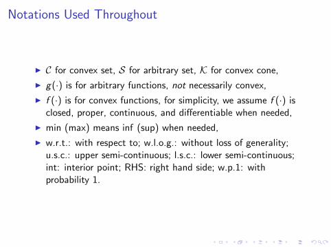
Notations Used Throughout

I C for convex set, S for arbitrary set, K for convex cone,

I g(·) is for arbitrary functions, not necessarily convex,

I f (·) is for convex functions, for simplicity, we assume f (·) isclosed, proper, continuous, and differentiable when needed,

I min (max) means inf (sup) when needed,

I w.r.t.: with respect to; w.l.o.g.: without loss of generality;u.s.c.: upper semi-continuous; l.s.c.: lower semi-continuous;int: interior point; RHS: right hand side; w.p.1: withprobability 1.

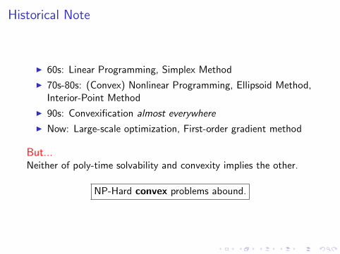
Historical Note

I 60s: Linear Programming, Simplex Method

I 70s-80s: (Convex) Nonlinear Programming, Ellipsoid Method,Interior-Point Method

I 90s: Convexification almost everywhere

I Now: Large-scale optimization, First-order gradient method

But...Neither of poly-time solvability and convexity implies the other.

NP-Hard convex problems abound.

Outline

Prelude

Basic Convex Analysis

Convex Optimization

Fenchel Conjugate

Minimax Theorem

Lagrangian Duality

References

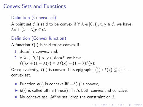
Convex Sets and Functions

Definition (Convex set)

A point set C is said to be convex if ∀ λ ∈ [0, 1], x , y ∈ C, we haveλx + (1− λ)y ∈ C.

Definition (Convex function)

A function f (·) is said to be convex if

1. domf is convex, and,

2. ∀ λ ∈ [0, 1], x , y ∈ domf , we havef (λx + (1− λ)y) ≤ λf (x) + (1− λ)f (y);

Or equivalently, f (·) is convex if its epigraph {(xt

): f (x) ≤ t} is a

convex set.

I Function h(·) is concave iff −h(·) is convex,

I h(·) is called affine (linear) iff it’s both convex and concave,

I No concave set. Affine set: drop the constraint on λ.

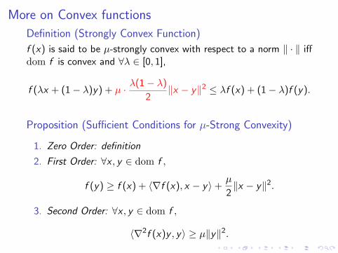
More on Convex functions

Definition (Strongly Convex Function)

f (x) is said to be µ-strongly convex with respect to a norm ‖ · ‖ iffdom f is convex and ∀λ ∈ [0, 1],

f (λx + (1− λ)y) + µ · λ(1− λ)

2‖x − y‖2 ≤ λf (x) + (1− λ)f (y).

Proposition (Sufficient Conditions for µ-Strong Convexity)

1. Zero Order: definition

2. First Order: ∀x , y ∈ dom f ,

f (y) ≥ f (x) + 〈∇f (x), x − y〉+µ

2‖x − y‖2.

3. Second Order: ∀x , y ∈ dom f ,

〈∇2f (x)y , y〉 ≥ µ‖y‖2.

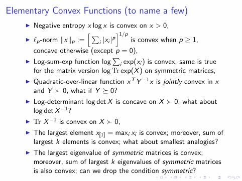
Elementary Convex Functions (to name a few)

I Negative entropy x log x is convex on x > 0,

I `p-norm ‖x‖p :=[∑

i |xi |p]1/p

is convex when p ≥ 1,

concave otherwise (except p = 0),

I Log-sum-exp function log∑

i exp(xi ) is convex, same is truefor the matrix version log Tr exp(X ) on symmetric matrices,

I Quadratic-over-linear function xT Y−1x is jointly convex in xand Y � 0, what if Y � 0?

I Log-determinant log det X is concave on X � 0, what aboutlog det X−1?

I Tr X−1 is convex on X � 0,

I The largest element x[1] = maxi xi is convex; moreover, sum oflargest k elements is convex; what about smallest analogies?

I The largest eigenvalue of symmetric matrices is convex;moreover, sum of largest k eigenvalues of symmetric matricesis also convex; can we drop the condition symmetric?

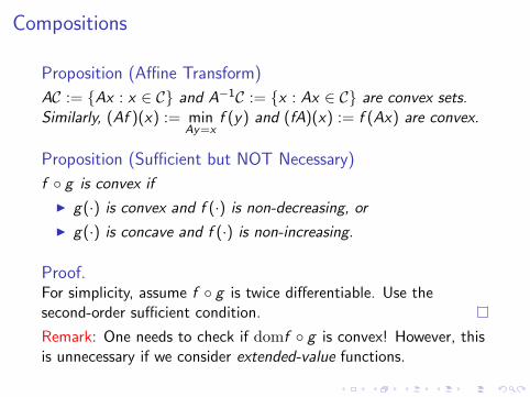
Compositions

Proposition (Affine Transform)

AC := {Ax : x ∈ C} and A−1C := {x : Ax ∈ C} are convex sets.Similarly, (Af )(x) := min

Ay=xf (y) and (fA)(x) := f (Ax) are convex.

Proposition (Sufficient but NOT Necessary)

f ◦ g is convex if

I g(·) is convex and f (·) is non-decreasing, or

I g(·) is concave and f (·) is non-increasing.

Proof.For simplicity, assume f ◦ g is twice differentiable. Use thesecond-order sufficient condition.

Remark: One needs to check if domf ◦ g is convex! However, thisis unnecessary if we consider extended-value functions.

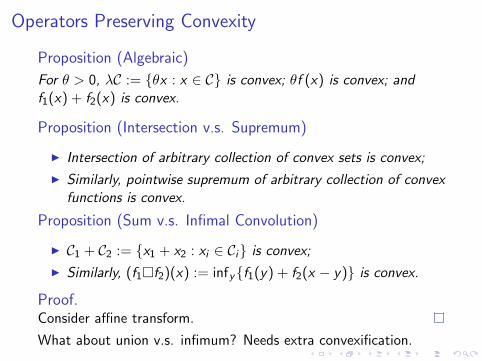
Operators Preserving Convexity

Proposition (Algebraic)

For θ > 0, λC := {θx : x ∈ C} is convex; θf (x) is convex; andf1(x) + f2(x) is convex.

Proposition (Intersection v.s. Supremum)

I Intersection of arbitrary collection of convex sets is convex;

I Similarly, pointwise supremum of arbitrary collection of convexfunctions is convex.

Proposition (Sum v.s. Infimal Convolution)

I C1 + C2 := {x1 + x2 : xi ∈ Ci} is convex;

I Similarly, (f1�f2)(x) := infy{f1(y) + f2(x − y)} is convex.

Proof.Consider affine transform.

What about union v.s. infimum? Needs extra convexification.

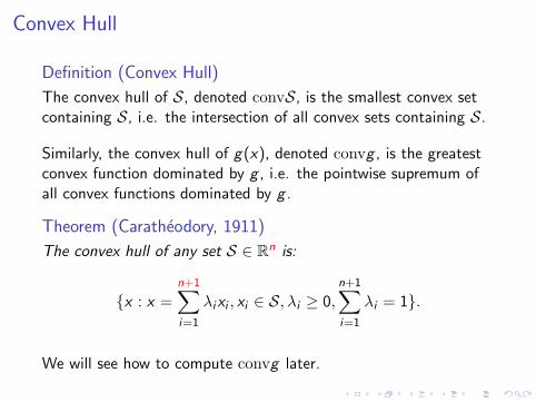
Convex Hull

Definition (Convex Hull)

The convex hull of S, denoted convS, is the smallest convex setcontaining S, i.e. the intersection of all convex sets containing S.

Similarly, the convex hull of g(x), denoted convg , is the greatestconvex function dominated by g , i.e. the pointwise supremum ofall convex functions dominated by g .

Theorem (Caratheodory, 1911)

The convex hull of any set S ∈ Rn is:

{x : x =n+1∑i=1

λixi , xi ∈ S, λi ≥ 0,n+1∑i=1

λi = 1}.

We will see how to compute convg later.

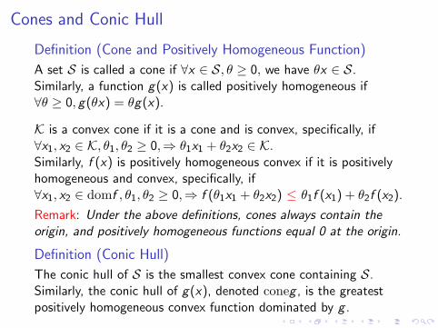
Cones and Conic Hull

Definition (Cone and Positively Homogeneous Function)

A set S is called a cone if ∀x ∈ S, θ ≥ 0, we have θx ∈ S.Similarly, a function g(x) is called positively homogeneous if∀θ ≥ 0, g(θx) = θg(x).

K is a convex cone if it is a cone and is convex, specifically, if∀x1, x2 ∈ K, θ1, θ2 ≥ 0,⇒ θ1x1 + θ2x2 ∈ K.Similarly, f (x) is positively homogeneous convex if it is positivelyhomogeneous and convex, specifically, if∀x1, x2 ∈ domf , θ1, θ2 ≥ 0,⇒ f (θ1x1 + θ2x2) ≤ θ1f (x1) + θ2f (x2).

Remark: Under the above definitions, cones always contain theorigin, and positively homogeneous functions equal 0 at the origin.

Definition (Conic Hull)

The conic hull of S is the smallest convex cone containing S.Similarly, the conic hull of g(x), denoted coneg , is the greatestpositively homogeneous convex function dominated by g .

Conic Hull cont’

Theorem (Caratheodory, 1911)

The conic hull of any set S ∈ Rn is:

{x : x =n∑

i=1

θixi , xi ∈ S, θi ≥ 0, }.

For convex function f (x), its conic hull is:

(conef )(x) = minθ≥0

θ · f (θ−1x).

How to compute coneg? Hint: coneg = cone convg , why?

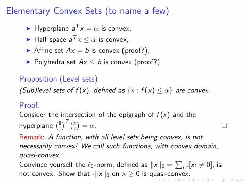
Elementary Convex Sets (to name a few)

I Hyperplane aT x = α is convex,

I Half space aT x ≤ α is convex,

I Affine set Ax = b is convex (proof?),

I Polyhedra set Ax ≤ b is convex (proof?),

Proposition (Level sets)

(Sub)level sets of f (x), defined as {x : f (x) ≤ α} are convex.

Proof.Consider the intersection of the epigraph of f (x) and the

hyperplane(0

1

)T (xt

)= α.

Remark: A function, with all level sets being convex, is notnecessarily convex! We call such functions, with convex domain,quasi-convex.Convince yourself the `0-norm, defined as ‖x‖0 =

∑i I[xi 6= 0], is

not convex. Show that -‖x‖0 on x ≥ 0 is quasi-convex.

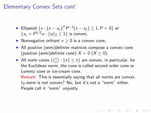
Elementary Convex Sets cont’

I Ellipsoid {x : (x − xc)T P−1(x − xc) ≤ 1,P � 0} or{xc + P1/2u : ‖u‖2 ≤ 1} is convex,

I Nonnegative orthant x ≥ 0 is a convex cone,

I All positive (semi)definite matrices compose a convex cone(positive (semi)definite cone) X � 0 (X � 0),

I All norm cones {(xt

): ‖x‖ ≤ t} are convex, in particular, for

the Euclidean norm, the cone is called second order cone orLorentz cone or ice-cream cone.Remark: This is essentially saying that all norms are convex.`0-norm is not convex? No, but it’s not a “norm” either.People call it “norm” unjustly.

Outline

Prelude

Basic Convex Analysis

Convex Optimization

Fenchel Conjugate

Minimax Theorem

Lagrangian Duality

References

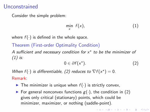
Unconstrained

Consider the simple problem:

minx

f (x), (1)

where f (·) is defined in the whole space.

Theorem (First-order Optimality Condition)

A sufficient and necessary condition for x? to be the minimizer of(1) is:

0 ∈ ∂f (x?). (2)

When f (·) is differentiable, (2) reduces to ∇f (x?) = 0.

Remark:

I The minimizer is unique when f (·) is strictly convex,

I For general nonconvex functions g(·), the condition in (2)gives only critical (stationary) points, which could beminimizer, maximizer, or nothing (saddle-point).

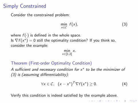
Simply Constrained

Consider the constrained problem:

minx∈C

f (x), (3)

where f (·) is defined in the whole space.Is ∇f (x?) = 0 still the optimality condition? If you think so,consider the example:

minx∈[1,2]

x .

Theorem (First-order Optimality Condition)

A sufficient and necessary condition for x? to be the minimizer of(3) is (assuming differentiability):

∀x ∈ C, (x − x?)T∇f (x?) ≥ 0. (4)

Verify this condition is indeed satisfied by the example above.

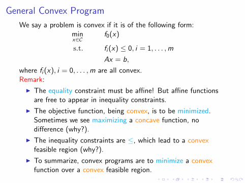
General Convex Program

We say a problem is convex if it is of the following form:minx∈C

f0(x)

s.t. fi (x) ≤ 0, i = 1, . . . ,m

Ax = b,

where fi (x), i = 0, . . . ,m are all convex.Remark:

I The equality constraint must be affine! But affine functionsare free to appear in inequality constraints.

I The objective function, being convex, is to be minimized.Sometimes we see maximizing a concave function, nodifference (why?).

I The inequality constraints are ≤, which lead to a convexfeasible region (why?).

I To summarize, convex programs are to minimize a convexfunction over a convex feasible region.

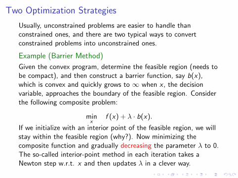
Two Optimization Strategies

Usually, unconstrained problems are easier to handle thanconstrained ones, and there are two typical ways to convertconstrained problems into unconstrained ones.

Example (Barrier Method)

Given the convex program, determine the feasible region (needs tobe compact), and then construct a barrier function, say b(x),which is convex and quickly grows to ∞ when x , the decisionvariable, approaches the boundary of the feasible region. Considerthe following composite problem:

minx

f (x) + λ · b(x).

If we initialize with an interior point of the feasible region, we willstay within the feasible region (why?). Now minimizing thecomposite function and gradually decreasing the parameter λ to 0.The so-called interior-point method in each iteration takes aNewton step w.r.t. x and then updates λ in a clever way.

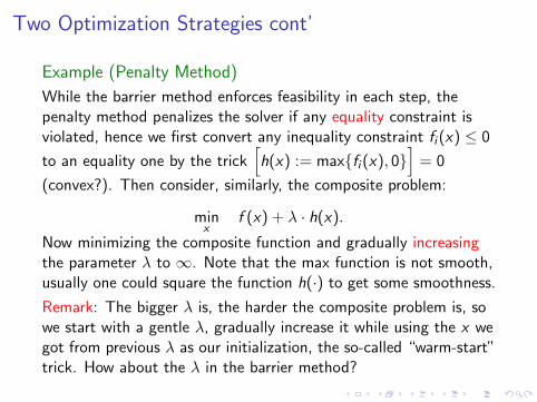
Two Optimization Strategies cont’

Example (Penalty Method)

While the barrier method enforces feasibility in each step, thepenalty method penalizes the solver if any equality constraint isviolated, hence we first convert any inequality constraint fi (x) ≤ 0

to an equality one by the trick[h(x) := max{fi (x), 0}

]= 0

(convex?). Then consider, similarly, the composite problem:

minx

f (x) + λ · h(x).

Now minimizing the composite function and gradually increasingthe parameter λ to ∞. Note that the max function is not smooth,usually one could square the function h(·) to get some smoothness.

Remark: The bigger λ is, the harder the composite problem is, sowe start with a gentle λ, gradually increase it while using the x wegot from previous λ as our initialization, the so-called “warm-start”trick. How about the λ in the barrier method?

Linear Programming (LP)

Standard Form

minx

cT x

s.t. x ≥ 0

Ax = b

General Form

minx

cT x

s.t. Bx ≤ d

Ax = b

Example (Piecewise-linear Minimization)

minx

f (x) := maxi

aTi x + bi

This does not look like an LP, but can be equivalently reformulatedas one:

minx ,t

t s.t. aTi x + bi ≤ t,∀i .

Remark: Important trick, learn it!

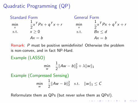
Quadratic Programming (QP)

Standard Form

minx

1

2xT Px + qT x + r

s.t. x ≥ 0

Ax = b

General Form

minx

1

2xT Px + qT x + r

s.t. Bx ≤ d

Ax = b

Remark: P must be positive semidefinite! Otherwise the problemis non-convex, and in fact NP-Hard.

Example (LASSO)

minw

1

2‖Aw − b‖2

2 + λ‖w‖1

Example (Compressed Sensing)

minw

1

2‖Aw − b‖2

2 s.t. ‖w‖1 ≤ C

Reformulate them as QPs (but never solve them as QPs!).

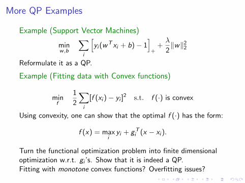
More QP Examples

Example (Support Vector Machines)

minw ,b

∑i

[yi (wT xi + b)− 1

]+

+λ

2‖w‖2

2

Reformulate it as a QP.

Example (Fitting data with Convex functions)

minf

1

2

∑i

[f (xi )− yi ]2 s.t. f (·) is convex

Using convexity, one can show that the optimal f (·) has the form:

f (x) = maxi

yi + gTi (x − xi ).

Turn the functional optimization problem into finite dimensionaloptimization w.r.t. gi ’s. Show that it is indeed a QP.Fitting with monotone convex functions? Overfitting issues?

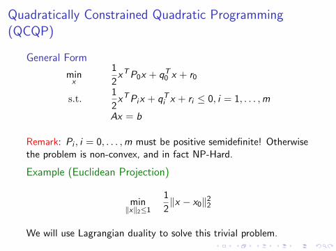
Quadratically Constrained Quadratic Programming(QCQP)

General Form

minx

1

2xT P0x + qT

0 x + r0

s.t.1

2xT Pix + qT

i x + ri ≤ 0, i = 1, . . . ,m

Ax = b

Remark: Pi , i = 0, . . . ,m must be positive semidefinite! Otherwisethe problem is non-convex, and in fact NP-Hard.

Example (Euclidean Projection)

min‖x‖2≤1

1

2‖x − x0‖2

2

We will use Lagrangian duality to solve this trivial problem.

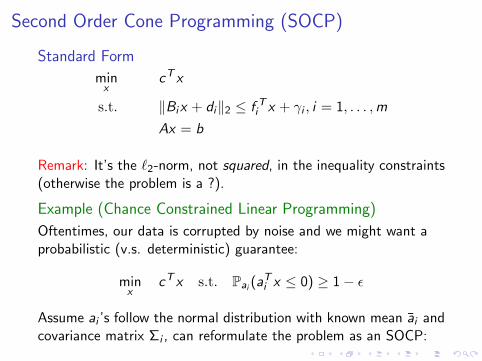
Second Order Cone Programming (SOCP)

Standard Form

minx

cT x

s.t. ‖Bix + di‖2 ≤ f Ti x + γi , i = 1, . . . ,m

Ax = b

Remark: It’s the `2-norm, not squared, in the inequality constraints(otherwise the problem is a ?).

Example (Chance Constrained Linear Programming)

Oftentimes, our data is corrupted by noise and we might want aprobabilistic (v.s. deterministic) guarantee:

minx

cT x s.t. Pai (aTi x ≤ 0) ≥ 1− ε

Assume ai ’s follow the normal distribution with known mean ai andcovariance matrix Σi , can reformulate the problem as an SOCP:

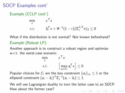
SOCP Examples cont’

Example (CCLP cont’)

minx

cT x

s.t. aTi x + Φ−1(1− ε)‖Σ1/2

i x‖2 ≤ 0

What if the distribution is not normal? Not known beforehand?

Example (Robust LP)

Another approach is to construct a robust region and optimizew.r.t. the worst-case scenario:

minx

cT x

s.t.[

maxai∈Ei

aTi x]≤ 0

Popular choices for Ei are the box constraint ‖ai‖∞ ≤ 1 or theellipsoid constraint (ai − ai )

T Σ−1i (ai − ai ) ≤ 1.

We will use Lagrangian duality to turn the latter case to an SOCP.How about the former case?

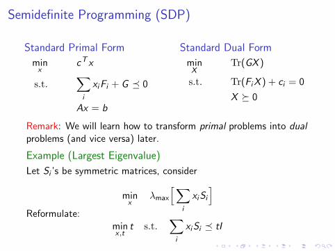
Semidefinite Programming (SDP)

Standard Primal Form

minx

cT x

s.t.∑

i

xiFi + G � 0

Ax = b

Standard Dual Form

minX

Tr(GX )

s.t. Tr(FiX ) + ci = 0

X � 0

Remark: We will learn how to transform primal problems into dualproblems (and vice versa) later.

Example (Largest Eigenvalue)

Let Si ’s be symmetric matrices, consider

minx

λmax

[∑i

xiSi

]Reformulate:

minx ,t

t s.t.∑

i

xiSi � tI

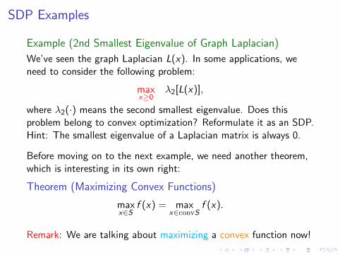
SDP Examples

Example (2nd Smallest Eigenvalue of Graph Laplacian)

We’ve seen the graph Laplacian L(x). In some applications, weneed to consider the following problem:

maxx≥0

λ2[L(x)],

where λ2(·) means the second smallest eigenvalue. Does thisproblem belong to convex optimization? Reformulate it as an SDP.Hint: The smallest eigenvalue of a Laplacian matrix is always 0.

Before moving on to the next example, we need another theorem,which is interesting in its own right:

Theorem (Maximizing Convex Functions)

maxx∈S

f (x) = maxx∈convS

f (x).

Remark: We are talking about maximizing a convex function now!

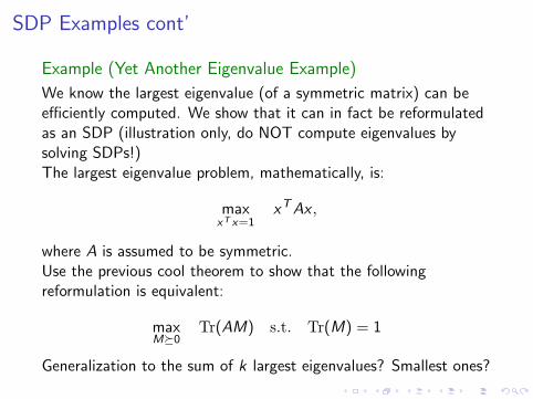
SDP Examples cont’

Example (Yet Another Eigenvalue Example)

We know the largest eigenvalue (of a symmetric matrix) can beefficiently computed. We show that it can in fact be reformulatedas an SDP (illustration only, do NOT compute eigenvalues bysolving SDPs!)The largest eigenvalue problem, mathematically, is:

maxxT x=1

xT Ax ,

where A is assumed to be symmetric.Use the previous cool theorem to show that the followingreformulation is equivalent:

maxM�0

Tr(AM) s.t. Tr(M) = 1

Generalization to the sum of k largest eigenvalues? Smallest ones?

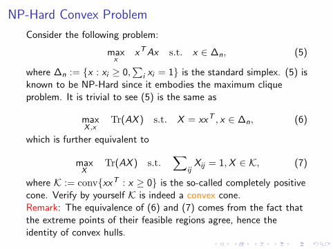
NP-Hard Convex Problem

Consider the following problem:

maxx

xT Ax s.t. x ∈ ∆n, (5)

where ∆n := {x : xi ≥ 0,∑

i xi = 1} is the standard simplex. (5) isknown to be NP-Hard since it embodies the maximum cliqueproblem. It is trivial to see (5) is the same as

maxX ,x

Tr(AX ) s.t. X = xxT , x ∈ ∆n, (6)

which is further equivalent to

maxX

Tr(AX ) s.t.∑

ijXij = 1,X ∈ K, (7)

where K := conv{xxT : x ≥ 0} is the so-called completely positivecone. Verify by yourself K is indeed a convex cone.Remark: The equivalence of (6) and (7) comes from the fact thatthe extreme points of their feasible regions agree, hence theidentity of convex hulls.

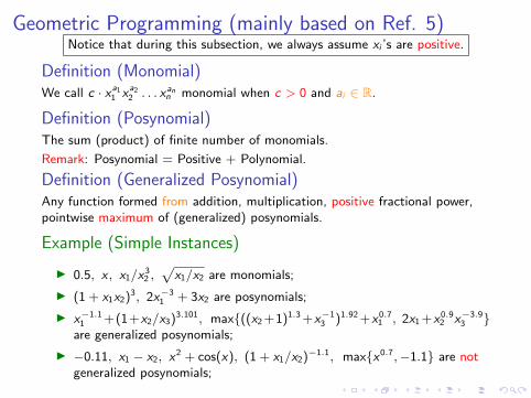
Geometric Programming (mainly based on Ref. 5)Notice that during this subsection, we always assume xi ’s are positive.

Definition (Monomial)We call c · xa1

1 xa22 . . . xan

n monomial when c > 0 and ai ∈ R.

Definition (Posynomial)The sum (product) of finite number of monomials.

Remark: Posynomial = Positive + Polynomial.

Definition (Generalized Posynomial)Any function formed from addition, multiplication, positive fractional power,pointwise maximum of (generalized) posynomials.

Example (Simple Instances)

I 0.5, x , x1/x32 ,

px1/x2 are monomials;

I (1 + x1x2)3, 2x−31 + 3x2 are posynomials;

I x−1.11 +(1+x2/x3)3.101, max{((x2 +1)1.3 +x−1

3 )1.92 +x0.71 , 2x1 +x0.9

2 x−3.93 }

are generalized posynomials;

I −0.11, x1 − x2, x2 + cos(x), (1 + x1/x2)−1.1, max{x0.7,−1.1} are notgeneralized posynomials;

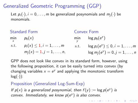
Generalized Geometric Programming (GGP)

Let pi (·), i = 0, . . . ,m be generalized posynomials and mj(·) bemonomials.

Standard Form

minx

p0(x)

s.t. pi (x) ≤ 1, i = 1, . . . ,m

mj(x) = 1, j = 1, . . . , n,

Convex Form

miny

log p0(ey )

s.t. log pi (ey ) ≤ 0, i = 1, . . . ,m

log mj(ey ) = 0, j = 1, . . . , n

GPP does not look like convex in its standard form, however, usingthe following proposition, it can be easily turned into convex (bychanging variables x = ey and applying the monotonic transformlog(·)):

Proposition (Generalized Log-Sum-Exp)

If p(x) is a generalized posynomial, then f (y) := log p(ey ) isconvex. Immediately, we know p(ey ) is also convex.

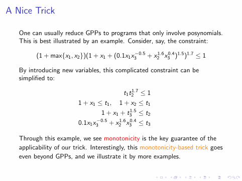
A Nice Trick

One can usually reduce GPPs to programs that only involve posynomials.This is best illustrated by an example. Consider, say, the constraint:

(1 + max{x1, x2})(1 + x1 + (0.1x1x−0.53 + x1.6

2 x0.43 )1.5)1.7 ≤ 1

By introducing new variables, this complicated constraint can besimplified to:

t1t1.72 ≤ 1

1 + x1 ≤ t1, 1 + x2 ≤ t1

1 + x1 + t1.53 ≤ t2

0.1x1x−0.53 + x1.6

2 x0.43 ≤ t3

Through this example, we see monotonicity is the key guarantee of the

applicability of our trick. Interestingly, this monotonicity-based trick goes

even beyond GPPs, and we illustrate it by more examples.

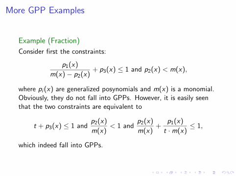
More GPP Examples

Example (Fraction)

Consider first the constraints:

p1(x)

m(x)− p2(x)+ p3(x) ≤ 1 and p2(x) < m(x),

where pi (x) are generalized posynomials and m(x) is a monomial.Obviously, they do not fall into GPPs. However, it is easily seenthat the two constraints are equivalent to

t + p3(x) ≤ 1 andp2(x)

m(x)< 1 and

p2(x)

m(x)+

p1(x)

t ·m(x)≤ 1,

which indeed fall into GPPs.

More GPP Examples cont’

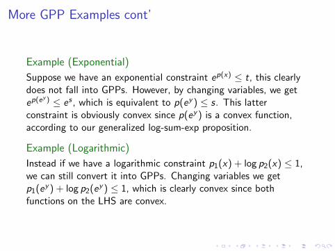
Example (Exponential)

Suppose we have an exponential constraint ep(x) ≤ t, this clearlydoes not fall into GPPs. However, by changing variables, we getep(ey ) ≤ es , which is equivalent to p(ey ) ≤ s. This latterconstraint is obviously convex since p(ey ) is a convex function,according to our generalized log-sum-exp proposition.

Example (Logarithmic)

Instead if we have a logarithmic constraint p1(x) + log p2(x) ≤ 1,we can still convert it into GPPs. Changing variables we getp1(ey ) + log p2(ey ) ≤ 1, which is clearly convex since bothfunctions on the LHS are convex.

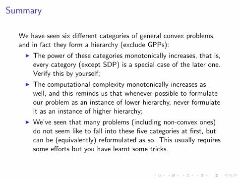
Summary

We have seen six different categories of general convex problems,and in fact they form a hierarchy (exclude GPPs):

I The power of these categories monotonically increases, that is,every category (except SDP) is a special case of the later one.Verify this by yourself;

I The computational complexity monotonically increases aswell, and this reminds us that whenever possible to formulateour problem as an instance of lower hierarchy, never formulateit as an instance of higher hierarchy;

I We’ve seen that many problems (including non-convex ones)do not seem like to fall into these five categories at first, butcan be (equivalently) reformulated as so. This usually requiressome efforts but you have learnt some tricks.

Outline

Prelude

Basic Convex Analysis

Convex Optimization

Fenchel Conjugate

Minimax Theorem

Lagrangian Duality

References

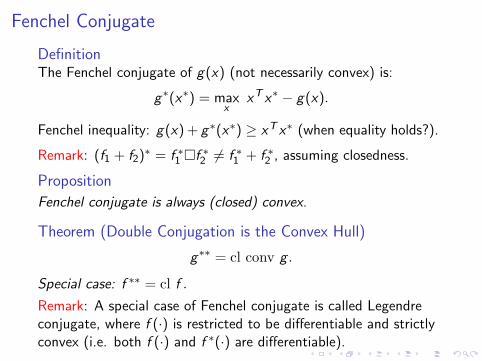
Fenchel Conjugate

DefinitionThe Fenchel conjugate of g(x) (not necessarily convex) is:

g∗(x∗) = maxx

xT x∗ − g(x).

Fenchel inequality: g(x) + g∗(x∗) ≥ xT x∗ (when equality holds?).

Remark: (f1 + f2)∗ = f ∗1 �f ∗2 6= f ∗1 + f ∗2 , assuming closedness.

Proposition

Fenchel conjugate is always (closed) convex.

Theorem (Double Conjugation is the Convex Hull)

g∗∗ = cl conv g .

Special case: f ∗∗ = cl f .

Remark: A special case of Fenchel conjugate is called Legendreconjugate, where f (·) is restricted to be differentiable and strictlyconvex (i.e. both f (·) and f ∗(·) are differentiable).

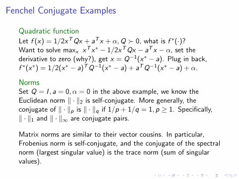
Fenchel Conjugate Examples

Quadratic functionLet f (x) = 1/2xT Qx + aT x + α,Q � 0, what is f ∗(·)?Want to solve maxx xT x∗ − 1/2xT Qx − aT x − α, set thederivative to zero (why?), get x = Q−1(x∗ − a). Plug in back,f ∗(x∗) = 1/2(x∗ − a)T Q−1(x∗ − a) + aT Q−1(x∗ − a) + α.

NormsSet Q = I , a = 0, α = 0 in the above example, we know theEuclidean norm ‖ · ‖2 is self-conjugate. More generally, theconjugate of ‖ · ‖p is ‖ · ‖q if 1/p + 1/q = 1, p ≥ 1. Specifically,‖ · ‖1 and ‖ · ‖∞ are conjugate pairs.

Matrix norms are similar to their vector cousins. In particular,Frobenius norm is self-conjugate, and the conjugate of the spectralnorm (largest singular value) is the trace norm (sum of singularvalues).

More Interesting Examples

In many cases, one really needs to minimize the `0-norm, which isunfortunately non-convex. The remedy is to instead minimize theso-called tightest convex approximation, namely, conv‖ · ‖0.

We’ve seen that g∗∗ = convg , so let’s compute conv‖ · ‖0.

Step 1: (‖ · ‖0)∗(x∗) = maxx xT x∗ − ‖x‖0 =

{0, x∗ = 0∞, otherwise

Step 2: (‖ · ‖0)∗∗(x) = maxx∗ xT x∗ − (‖ · ‖0)∗(x∗) = 0.

Hence, (conv‖ · ‖0)(x) = 0 ! Is this correct? Draw a graph toverify. Is this a meaningful surrogate for ‖ · ‖0? Not really...

Stare at the graph you drew. What prevents us from obtaining ameaningful surrogate? How to get around?

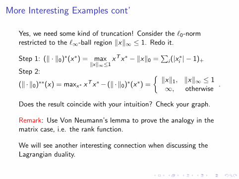
More Interesting Examples cont’

Yes, we need some kind of truncation! Consider the `0-normrestricted to the `∞-ball region ‖x‖∞ ≤ 1. Redo it.

Step 1: (‖ · ‖0)∗(x∗) = max‖x‖∞≤1

xT x∗ − ‖x‖0 =∑

i (|x∗i | − 1)+

Step 2:

(‖ · ‖0)∗∗(x) = maxx∗ xT x∗− (‖ · ‖0)∗(x∗) =

{‖x‖1, ‖x‖∞ ≤ 1∞, otherwise

.

Does the result coincide with your intuition? Check your graph.

Remark: Use Von Neumann’s lemma to prove the analogy in thematrix case, i.e. the rank function.

We will see another interesting connection when discussing theLagrangian duality.

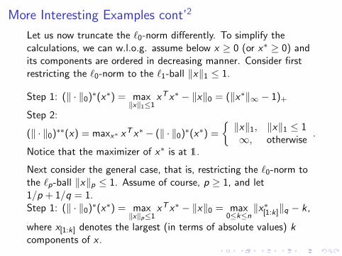
More Interesting Examples cont’2

Let us now truncate the `0-norm differently. To simplify thecalculations, we can w.l.o.g. assume below x ≥ 0 (or x∗ ≥ 0) andits components are ordered in decreasing manner. Consider firstrestricting the `0-norm to the `1-ball ‖x‖1 ≤ 1.

Step 1: (‖ · ‖0)∗(x∗) = max‖x‖1≤1

xT x∗ − ‖x‖0 = (‖x∗‖∞ − 1)+

Step 2:

(‖ · ‖0)∗∗(x) = maxx∗ xT x∗ − (‖ · ‖0)∗(x∗) =

{‖x‖1, ‖x‖1 ≤ 1∞, otherwise

.

Notice that the maximizer of x∗ is at 1.

Next consider the general case, that is, restricting the `0-norm tothe `p-ball ‖x‖p ≤ 1. Assume of course, p ≥ 1, and let1/p + 1/q = 1.Step 1: (‖ · ‖0)∗(x∗) = max

‖x‖p≤1xT x∗ − ‖x‖0 = max

0≤k≤n‖x∗[1:k]‖q − k ,

where x[1:k] denotes the largest (in terms of absolute values) kcomponents of x .

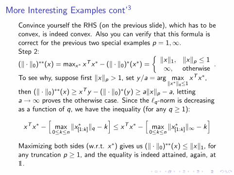
More Interesting Examples cont’3

Convince yourself the RHS (on the previous slide), which has to beconvex, is indeed convex. Also you can verify that this formula iscorrect for the previous two special examples p = 1,∞.Step 2:

(‖ · ‖0)∗∗(x) = maxx∗ xT x∗ − (‖ · ‖0)∗(x∗) =

{‖x‖1, ‖x‖p ≤ 1∞, otherwise

.

To see why, suppose first ‖x‖p > 1, set y/a = arg max‖x∗‖q≤1

xT x∗,

then (‖ · ‖0)∗∗(x) ≥ xT y − (‖ · ‖0)∗(y) ≥ a‖x‖p − a, lettinga→∞ proves the otherwise case. Since the `q-norm is decreasingas a function of q, we have the inequality (for any q ≥ 1):

xT x∗ −[

max0≤k≤n

‖x∗[1:k]‖q − k]≤ xT x∗ −

[max

0≤k≤n‖x∗[1:k]‖∞ − k

]Maximizing both sides (w.r.t. x∗) gives us (‖ · ‖0)∗∗(x) ≤ ‖x‖1, forany truncation p ≥ 1, and the equality is indeed attained, again, at1.

Outline

Prelude

Basic Convex Analysis

Convex Optimization

Fenchel Conjugate

Minimax Theorem

Lagrangian Duality

References

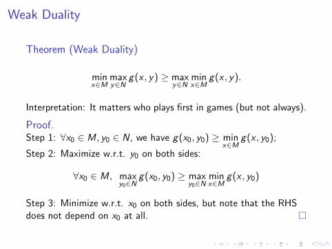
Weak Duality

Theorem (Weak Duality)

minx∈M

maxy∈N

g(x , y) ≥ maxy∈N

minx∈M

g(x , y).

Interpretation: It matters who plays first in games (but not always).

Proof.Step 1: ∀x0 ∈ M, y0 ∈ N, we have g(x0, y0) ≥ min

x∈Mg(x , y0);

Step 2: Maximize w.r.t. y0 on both sides:

∀x0 ∈ M, maxy0∈N

g(x0, y0) ≥ maxy0∈N

minx∈M

g(x , y0)

Step 3: Minimize w.r.t. x0 on both sides, but note that the RHSdoes not depend on x0 at all.

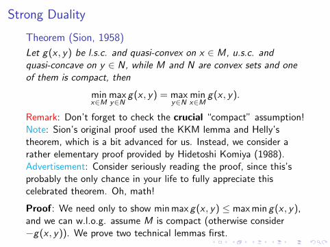
Strong Duality

Theorem (Sion, 1958)

Let g(x , y) be l.s.c. and quasi-convex on x ∈ M, u.s.c. andquasi-concave on y ∈ N, while M and N are convex sets and oneof them is compact, then

minx∈M

maxy∈N

g(x , y) = maxy∈N

minx∈M

g(x , y).

Remark: Don’t forget to check the crucial “compact” assumption!Note: Sion’s original proof used the KKM lemma and Helly’stheorem, which is a bit advanced for us. Instead, we consider arather elementary proof provided by Hidetoshi Komiya (1988).Advertisement: Consider seriously reading the proof, since this’sprobably the only chance in your life to fully appreciate thiscelebrated theorem. Oh, math!

Proof: We need only to show min max g(x , y) ≤ max min g(x , y),and we can w.l.o.g. assume M is compact (otherwise consider−g(x , y)). We prove two technical lemmas first.

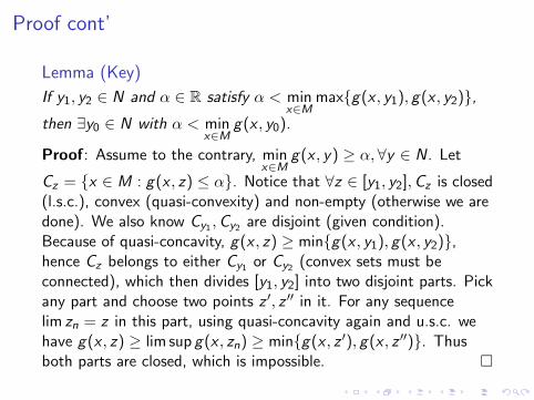
Proof cont’

Lemma (Key)

If y1, y2 ∈ N and α ∈ R satisfy α < minx∈M

max{g(x , y1), g(x , y2)},then ∃y0 ∈ N with α < min

x∈Mg(x , y0).

Proof: Assume to the contrary, minx∈M

g(x , y) ≥ α,∀y ∈ N. Let

Cz = {x ∈ M : g(x , z) ≤ α}. Notice that ∀z ∈ [y1, y2],Cz is closed(l.s.c.), convex (quasi-convexity) and non-empty (otherwise we aredone). We also know Cy1 ,Cy2 are disjoint (given condition).Because of quasi-concavity, g(x , z) ≥ min{g(x , y1), g(x , y2)},hence Cz belongs to either Cy1 or Cy2 (convex sets must beconnected), which then divides [y1, y2] into two disjoint parts. Pickany part and choose two points z ′, z ′′ in it. For any sequencelim zn = z in this part, using quasi-concavity again and u.s.c. wehave g(x , z) ≥ lim sup g(x , zn) ≥ min{g(x , z ′), g(x , z ′′)}. Thusboth parts are closed, which is impossible. �

Proof cont’2

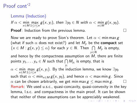
Lemma (Induction)

If α < minx∈M

max1≤i≤n

g(x , yi ), then ∃y0 ∈ N with α < minx∈M

g(x , y0).

Proof: Induction from the previous lemma. �

Now we are ready to prove Sion’s theorem. Let α < min max g(what if such α does not exist?) and let My be the compact set{x ∈ M : g(x , y) ≤ α} for each y ∈ N. Then

⋂y∈N

My is empty,

and hence by the compactness assumption on M, there are finitepoints y1, . . . yn ∈ N such that

⋂yi

Myi is empty, that is

α < minx∈M

max1≤i≤n

g(x , yi ). By the induction lemma, we know ∃y0

such that α < minx∈M g(x , y0), and hence α < max min g . Sinceα can be chosen arbitrarily, we get min max g ≤ max min g . �Remark: We used u.s.c., quasi-concavity, quasi-convexity in the keylemma, l.s.c. and compactness in the main proof. It can be shownthat neither of these assumptions can be appreciably weakened.

Variations

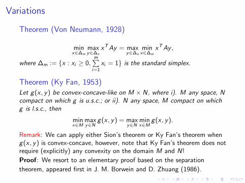
Theorem (Von Neumann, 1928)

minx∈∆m

maxy∈∆n

xT Ay = maxy∈∆n

minx∈∆m

xT Ay ,

where ∆m := {x : xi ≥ 0,m∑

i=1

xi = 1} is the standard simplex.

Theorem (Ky Fan, 1953)Let g(x , y) be convex-concave-like on M × N, where i). M any space, Ncompact on which g is u.s.c.; or ii). N any space, M compact on whichg is l.s.c., then

minx∈M

maxy∈N

g(x , y) = maxy∈N

minx∈M

g(x , y).

Remark: We can apply either Sion’s theorem or Ky Fan’s theorem wheng(x , y) is convex-concave, however, note that Ky Fan’s theorem does notrequire (explicitly) any convexity on the domain M and N!

Proof: We resort to an elementary proof based on the separation

theorem, appeared first in J. M. Borwein and D. Zhuang (1986).

Variations cont’

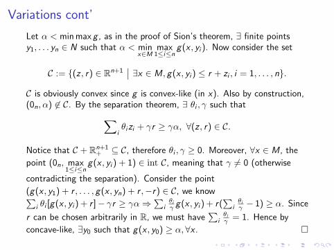
Let α < min max g , as in the proof of Sion’s theorem, ∃ finite pointsy1, . . . yn ∈ N such that α < min

x∈Mmax

1≤i≤ng(x , yi ). Now consider the set

C := {(z , r) ∈ Rn+1∣∣ ∃x ∈ M, g(x , yi ) ≤ r + zi , i = 1, . . . , n}.

C is obviously convex since g is convex-like (in x). Also by construction,(0n, α) 6∈ C. By the separation theorem, ∃ θi , γ such that∑

iθizi + γr ≥ γα, ∀(z , r) ∈ C.

Notice that C + Rn+1+ ⊆ C, therefore θi , γ ≥ 0. Moreover, ∀x ∈ M, the

point (0n, max1≤i≤n

g(x , yi ) + 1) ∈ int C, meaning that γ 6= 0 (otherwise

contradicting the separation). Consider the point

(g(x , y1) + r , . . . , g(x , yn) + r ,−r) ∈ C, we know∑i θi [g(x , yi ) + r ]− γr ≥ γα⇒

∑iθi

γ g(x , yi ) + r(∑

iθi

γ − 1) ≥ α. Since

r can be chosen arbitrarily in R, we must have∑

iθi

γ = 1. Hence by

concave-like, ∃y0 such that g(x , y0) ≥ α,∀x . �

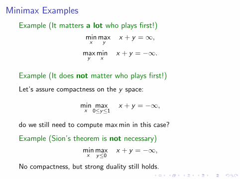
Minimax Examples

Example (It matters a lot who plays first!)

minx

maxy

x + y =∞,

maxy

minx

x + y = −∞.

Example (It does not matter who plays first!)

Let’s assure compactness on the y space:

minx

max0≤y≤1

x + y = −∞,

do we still need to compute max min in this case?

Example (Sion’s theorem is not necessary)

minx

maxy≤0

x + y = −∞,

No compactness, but strong duality still holds.

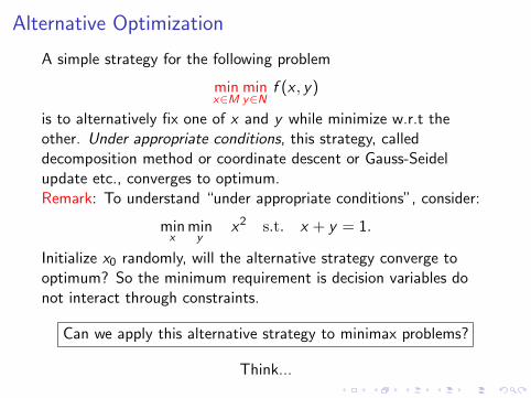
Alternative Optimization

A simple strategy for the following problem

minx∈M

miny∈N

f (x , y)

is to alternatively fix one of x and y while minimize w.r.t theother. Under appropriate conditions, this strategy, calleddecomposition method or coordinate descent or Gauss-Seidelupdate etc., converges to optimum.Remark: To understand “under appropriate conditions”, consider:

minx

miny

x2 s.t. x + y = 1.

Initialize x0 randomly, will the alternative strategy converge tooptimum? So the minimum requirement is decision variables donot interact through constraints.

Can we apply this alternative strategy to minimax problems?

Think...

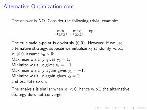
Alternative Optimization cont’

The answer is NO. Consider the following trivial example:

min−1≤x≤1

max−1≤y≤1

xy

The true saddle-point is obviously (0,0). However, if we usealternative strategy, suppose we initialize x0 randomly, w.p.1x0 6= 0, assume x0 > 0:Maximize w.r.t. y gives y0 = 1;Minimize w.r.t. x gives x1 = −1;Maximize w.r.t. y again gives y1 = −1;Minimize w.r.t. x again gives x2 = 1;and oscillate so on.

The analysis is similar when x0 < 0, hence w.p.1 the alternativestrategy does not converge!

Outline

Prelude

Basic Convex Analysis

Convex Optimization

Fenchel Conjugate

Minimax Theorem

Lagrangian Duality

References

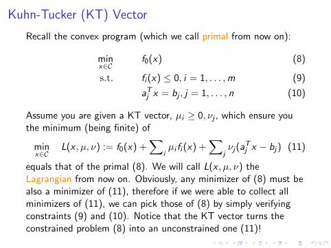
Kuhn-Tucker (KT) Vector

Recall the convex program (which we call primal from now on):

minx∈C

f0(x) (8)

s.t. fi (x) ≤ 0, i = 1, . . . ,m (9)

aTj x = bj , j = 1, . . . , n (10)

Assume you are given a KT vector, µi ≥ 0, νj , which ensure youthe minimum (being finite) of

minx∈C

L(x , µ, ν) := f0(x) +∑

iµi fi (x) +

∑jνj(aT

j x − bj) (11)

equals that of the primal (8). We will call L(x , µ, ν) theLagrangian from now on. Obviously, any minimizer of (8) must bealso a minimizer of (11), therefore if we were able to collect allminimizers of (11), we can pick those of (8) by simply verifyingconstraints (9) and (10). Notice that the KT vector turns theconstrained problem (8) into an unconstrained one (11)!

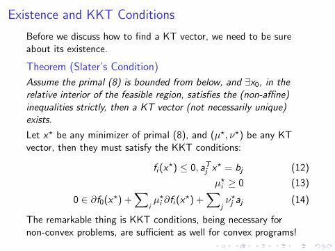
Existence and KKT Conditions

Before we discuss how to find a KT vector, we need to be sureabout its existence.

Theorem (Slater’s Condition)

Assume the primal (8) is bounded from below, and ∃x0, in therelative interior of the feasible region, satisfies the (non-affine)inequalities strictly, then a KT vector (not necessarily unique)exists.

Let x? be any minimizer of primal (8), and (µ?, ν?) be any KTvector, then they must satisfy the KKT conditions:

fi (x?) ≤ 0, aTj x? = bj (12)

µ?i ≥ 0 (13)

0 ∈ ∂f0(x?) +∑

iµ?i ∂fi (x?) +

∑jν?j aj (14)

The remarkable thing is KKT conditions, being necessary fornon-convex problems, are sufficient as well for convex programs!

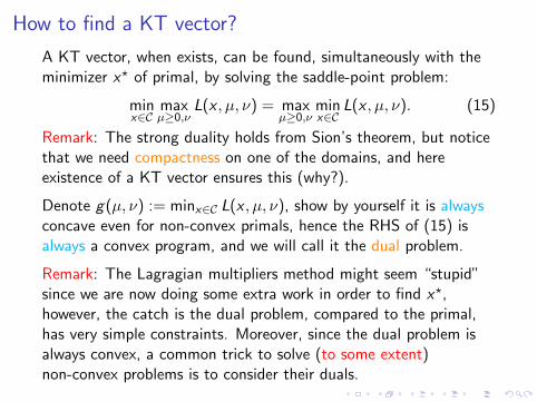
How to find a KT vector?

A KT vector, when exists, can be found, simultaneously with theminimizer x? of primal, by solving the saddle-point problem:

minx∈C

maxµ≥0,ν

L(x , µ, ν) = maxµ≥0,ν

minx∈C

L(x , µ, ν). (15)

Remark: The strong duality holds from Sion’s theorem, but noticethat we need compactness on one of the domains, and hereexistence of a KT vector ensures this (why?).

Denote g(µ, ν) := minx∈C L(x , µ, ν), show by yourself it is alwaysconcave even for non-convex primals, hence the RHS of (15) isalways a convex program, and we will call it the dual problem.

Remark: The Lagragian multipliers method might seem “stupid”since we are now doing some extra work in order to find x?,however, the catch is the dual problem, compared to the primal,has very simple constraints. Moreover, since the dual problem isalways convex, a common trick to solve (to some extent)non-convex problems is to consider their duals.

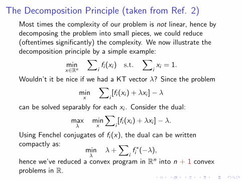
The Decomposition Principle (taken from Ref. 2)

Most times the complexity of our problem is not linear, hence bydecomposing the problem into small pieces, we could reduce(oftentimes significantly) the complexity. We now illustrate thedecomposition principle by a simple example:

minx∈Rn

∑ifi (xi ) s.t.

∑ixi = 1.

Wouldn’t it be nice if we had a KT vector λ? Since the problem

minx

∑i[fi (xi ) + λxi ]− λ

can be solved separably for each xi . Consider the dual:

maxλ

minx

∑i[fi (xi ) + λxi ]− λ.

Using Fenchel conjugates of fi (x), the dual can be writtencompactly as:

minλ

λ+∑

if ∗i (−λ),

hence we’ve reduced a convex program in Rn into n + 1 convexproblems in R.

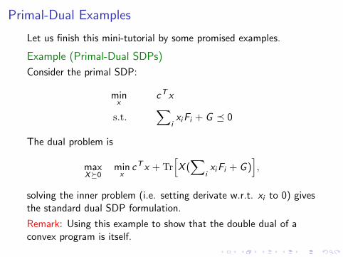
Primal-Dual Examples

Let us finish this mini-tutorial by some promised examples.

Example (Primal-Dual SDPs)

Consider the primal SDP:

minx

cT x

s.t.∑

ixiFi + G � 0

The dual problem is

maxX�0

minx

cT x + Tr[X (∑

ixiFi + G )

],

solving the inner problem (i.e. setting derivate w.r.t. xi to 0) givesthe standard dual SDP formulation.

Remark: Using this example to show that the double dual of aconvex program is itself.

Primal-Dual Examples cont’

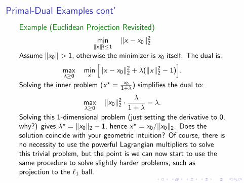
Example (Euclidean Projection Revisited)

min‖x‖2

2≤1‖x − x0‖2

2

Assume ‖x0‖ > 1, otherwise the minimizer is x0 itself. The dual is:

maxλ≥0

minx

[‖x − x0‖2

2 + λ(‖x‖22 − 1)

].

Solving the inner problem (x? = x01+λ) simplifies the dual to:

maxλ≥0

‖x0‖22 ·

λ

1 + λ− λ.

Solving this 1-dimensional problem (just setting the derivative to 0,why?) gives λ? = ‖x0‖2 − 1, hence x? = x0/‖x0‖2. Does thesolution coincide with your geometric intuition? Of course, there isno necessity to use the powerful Lagrangian multipliers to solvethis trivial problem, but the point is we can now start to use thesame procedure to solve slightly harder problems, such asprojection to the `1 ball.

Primal-Dual Examples cont’2

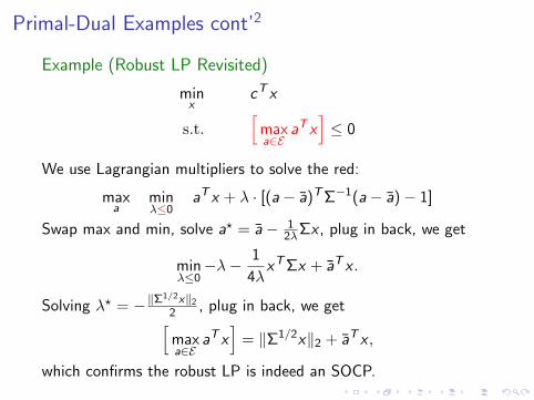
Example (Robust LP Revisited)

minx

cT x

s.t.[

maxa∈E

aT x]≤ 0

We use Lagrangian multipliers to solve the red:

maxa

minλ≤0

aT x + λ · [(a− a)T Σ−1(a− a)− 1]

Swap max and min, solve a? = a− 12λΣx , plug in back, we get

minλ≤0−λ− 1

4λxT Σx + aT x .

Solving λ? = −‖Σ1/2x‖2

2 , plug in back, we get[maxa∈E

aT x]

= ‖Σ1/2x‖2 + aT x ,

which confirms the robust LP is indeed an SOCP.

Outline

Prelude

Basic Convex Analysis

Convex Optimization

Fenchel Conjugate

Minimax Theorem

Lagrangian Duality

References

References

1. Introductory convex optimization book:Stephen Boyd and Lieven Vandenberghe. Convex Optimization. CambridgeUniversity Press, 2004.

2. Great book on convex analysis:Ralph T. Rockafellar. Convex Analysis. Princeton University Press, 1970.

3. Nice introduction of optimization strategies:Yurii Nesterov. Introductory Lectures on Convex Optimization: A Basic Course.Kluwer Academic Publishers, 2003.

4. The NP-Hard convex example is taken from:Mirjam Dur. Copositive Programming: A Survey. Manuscript, 2009.

5. The GPP subsection are mainly based on:Stephen Boyd, Seung-Jean Kim, Lieven Vandenberghe and Arash Hassibi. ATutorial on Geometric Programming. Optimization & Engineering. vol. 8, pp.67-127, 2007.

6. The proof of Sion’s theorem is mainly taken from:Hidetoshi Komiya. Elementary proof for Sion’s minimax theorem. KodaiMathematical Journal. vol. 11, no. 1, pp. 5-7, 1988.

7. The proof of Ky Fan’s theorem is mainly taken from:J. M. Bowrein and D. Zhuang. On Fan’s Minimax Theorem. MathematicalProgramming. vol. 34, pp. 232-234, 1986.