Embed Size (px)
Citation preview
XY-pic Reference Manual
Kristoffer H. Rose〈[email protected]〉×
Ross Moore〈[email protected]〉†
Version 3.7 〈1999/02/16〉
Abstract
This document summarises the capabilities of the XY-picpackage for typesetting graphs and diagrams in TEX. Fora general introduction as well as availability informationand conditions refer to the User’s Guide [14].
A characteristic of XY-pic is that it is built around akernel drawing language which is a concise notation forgeneral graphics, e.g.,
A
B(/).*-+,jjjjjjjjjG' 55
was drawn by the XY-pic kernel code
\xy (3,0)*{A} ; (20,6)*+{B}*\cir{} **\dir{-}
? *_!/3pt/\dir{)} *_!/7pt/\dir{:}
?>* \dir{>} \endxy
It is an object-oriented graphic language in the most lit-eral sense: ‘objects’ in the picture have ‘methods’ describ-ing how they typeset, stretch, etc. However, the syntaxis rather terse.
Particular applications make use of extensions thatenhance the graphic capabilities of the kernel to handlesuch diagrams as
Roundgfed`abc_^]\XYZ[Square
Bend
&&
which was typeset by
\xy *[o]=<40pt>\hbox{Round}="o"*\frm{oo},
+<5em,-5em>@+,
(46,11)*+\hbox{Square}="s" *\frm{-,},
-<5em,-5em>@+,
"o";"s" **{} ?*+\hbox{Bend}="b"*\frm{.},
"o";"s"."b" **\crvs{-},
"o"."b";"s" **\crvs{-} ?>*\dir{>}
\endxy
using the ‘curve’ and ‘frame’ extensions.All this is made accessible through the use of features
that provide convenient notation such that users can en-ter special classes of diagrams in an intuitive form, e.g.,
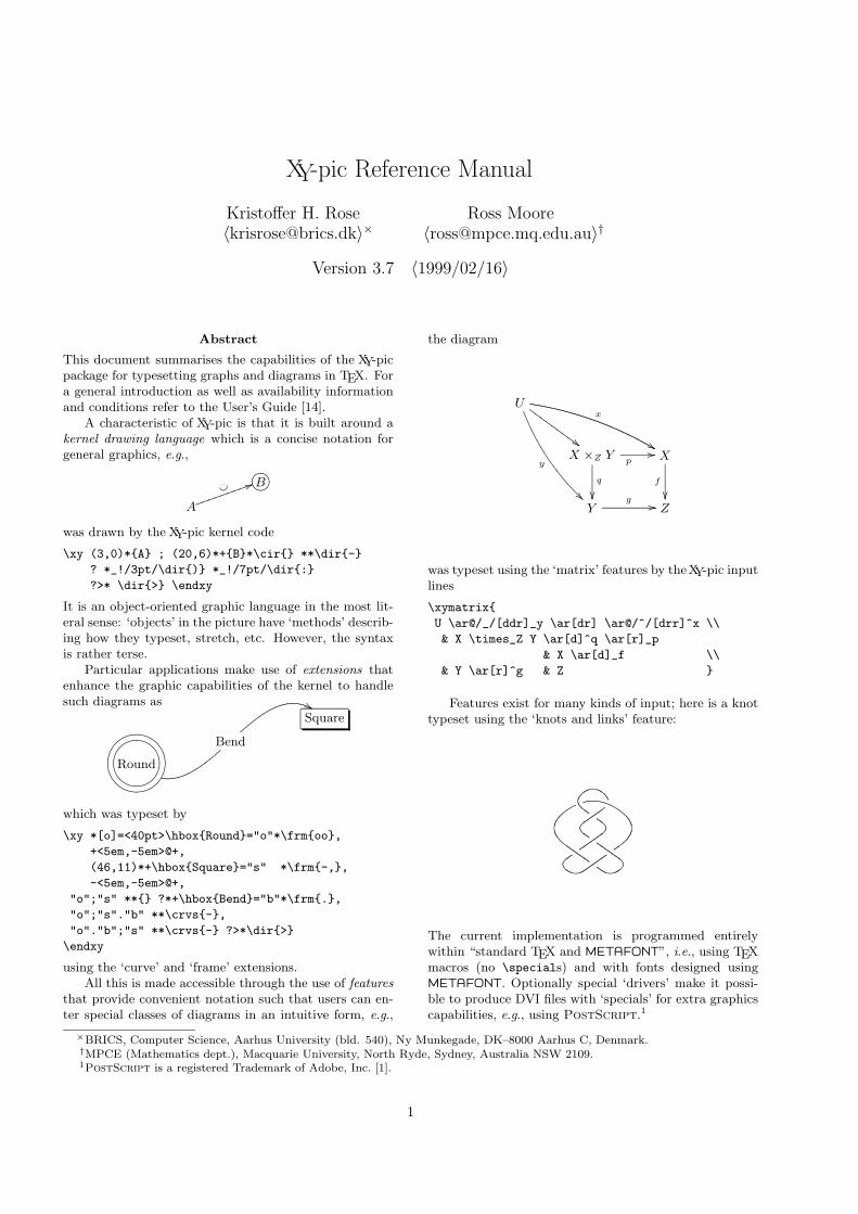
the diagram
U
y
##HHHHHHHHHx
%%X ×Z Y
q
��
p// X
f
��Y
g // Z
was typeset using the ‘matrix’ features by the XY-pic inputlines
\xymatrix{
U \ar@/_/[ddr]_y \ar[dr] \ar@/^/[drr]^x \\
& X \times_Z Y \ar[d]^q \ar[r]_p
& X \ar[d]_f \\
& Y \ar[r]^g & Z }
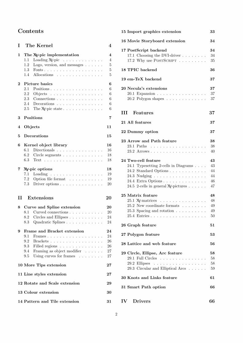
Features exist for many kinds of input; here is a knottypeset using the ‘knots and links’ feature:
The current implementation is programmed entirelywithin “standard TEX and METAFONT”, i.e., using TEXmacros (no \specials) and with fonts designed usingMETAFONT. Optionally special ‘drivers’ make it possi-ble to produce DVI files with ‘specials’ for extra graphicscapabilities, e.g., using PostScript.1
×BRICS, Computer Science, Aarhus University (bld. 540), Ny Munkegade, DK–8000 Aarhus C, Denmark.†MPCE (Mathematics dept.), Macquarie University, North Ryde, Sydney, Australia NSW 2109.1PostScript is a registered Trademark of Adobe, Inc. [1].
1
Contents
I The Kernel 4
1 The XY-pic implementation 41.1 Loading XY-pic . . . . . . . . . . . . . 41.2 Logo, version, and messages . . . . . . 51.3 Fonts . . . . . . . . . . . . . . . . . . . 51.4 Allocations . . . . . . . . . . . . . . . 5
2 Picture basics 62.1 Positions . . . . . . . . . . . . . . . . . 62.2 Objects . . . . . . . . . . . . . . . . . 62.3 Connections . . . . . . . . . . . . . . . 62.4 Decorations . . . . . . . . . . . . . . . 62.5 The XY-pic state . . . . . . . . . . . . . 6
3 Positions 7
4 Objects 11
5 Decorations 15
6 Kernel object library 166.1 Directionals . . . . . . . . . . . . . . . 166.2 Circle segments . . . . . . . . . . . . . 186.3 Text . . . . . . . . . . . . . . . . . . . 18
7 XY-pic options 187.1 Loading . . . . . . . . . . . . . . . . . 197.2 Option file format . . . . . . . . . . . 197.3 Driver options . . . . . . . . . . . . . . 20
II Extensions 20
8 Curve and Spline extension 208.1 Curved connections . . . . . . . . . . . 208.2 Circles and Ellipses . . . . . . . . . . . 248.3 Quadratic Splines . . . . . . . . . . . . 24
9 Frame and Bracket extension 249.1 Frames . . . . . . . . . . . . . . . . . . 249.2 Brackets . . . . . . . . . . . . . . . . . 269.3 Filled regions . . . . . . . . . . . . . . 269.4 Framing as object modifier . . . . . . 279.5 Using curves for frames . . . . . . . . 27
10 More Tips extension 27
11 Line styles extension 27
12 Rotate and Scale extension 29
13 Colour extension 30
14 Pattern and Tile extension 31
15 Import graphics extension 33
16 Movie Storyboard extension 34
17 PostScript backend 3417.1 Choosing the DVI-driver . . . . . . . . 3417.2 Why use PostScript . . . . . . . . . 35
18 TPIC backend 36
19 em-TeX backend 37
20 Necula’s extensions 3720.1 Expansion . . . . . . . . . . . . . . . . 3720.2 Polygon shapes . . . . . . . . . . . . . 37
III Features 37
21 All features 37
22 Dummy option 37
23 Arrow and Path feature 3823.1 Paths . . . . . . . . . . . . . . . . . . 3823.2 Arrows . . . . . . . . . . . . . . . . . . 40
24 Two-cell feature 4324.1 Typesetting 2-cells in Diagrams . . . . 4324.2 Standard Options . . . . . . . . . . . . 4424.3 Nudging . . . . . . . . . . . . . . . . . 4424.4 Extra Options . . . . . . . . . . . . . . 4624.5 2-cells in general XY-pictures . . . . . . 47
25 Matrix feature 4825.1 XY-matrices . . . . . . . . . . . . . . . 4825.2 New coordinate formats . . . . . . . . 4925.3 Spacing and rotation . . . . . . . . . . 4925.4 Entries . . . . . . . . . . . . . . . . . . 50
26 Graph feature 51
27 Polygon feature 53
28 Lattice and web feature 56
29 Circle, Ellipse, Arc feature 5829.1 Full Circles . . . . . . . . . . . . . . . 5829.2 Ellipses . . . . . . . . . . . . . . . . . 5829.3 Circular and Elliptical Arcs . . . . . . 59
30 Knots and Links feature 61
31 Smart Path option 66
IV Drivers 66
2
32 Support for Specific Drivers 6632.1 dvidrv driver . . . . . . . . . . . . . . 6632.2 DVIPS driver . . . . . . . . . . . . . . 6632.3 DVITOPS driver . . . . . . . . . . . . 6732.4 OzTeX driver . . . . . . . . . . . . . . 6732.5 OzTeX v1.7 driver . . . . . . . . . . . 6732.6 Textures driver . . . . . . . . . . . . . 6832.7 Textures v1.6 driver . . . . . . . . . . 6832.8 XDVI driver . . . . . . . . . . . . . . . 6832.9 CMacTeX driver . . . . . . . . . . . . 69
33 Extra features using PostScript drivers 6933.1 Colour . . . . . . . . . . . . . . . . . . 7033.2 Frames . . . . . . . . . . . . . . . . . . 7033.3 Line-styles . . . . . . . . . . . . . . . . 7033.4 Rotations and scaling . . . . . . . . . 7033.5 Patterns and tiles . . . . . . . . . . . . 71
34 Extra features using tpic drivers 7134.1 frames. . . . . . . . . . . . . . . . . . . 71
Appendices 71
A Answers to all exercises 71
B Version 2 Compatibility 75B.1 Unsupported incompatibilities . . . . . 75B.2 Obsolete kernel features . . . . . . . . 75B.3 Obsolete extensions & features . . . . 76B.4 Obsolete loading . . . . . . . . . . . . 77B.5 Compiling v2-diagrams . . . . . . . . . 77
C Common Errors 77
References 77
Index 78
List of Figures
1 〈pos〉itions. . . . . . . . . . . . . . . . 82 Example 〈place〉s . . . . . . . . . . . . 103 〈object〉s. . . . . . . . . . . . . . . . . 124 〈decor〉ations. . . . . . . . . . . . . . . 165 Kernel library 〈dir〉ectionals . . . . . . 176 〈cir〉cles. . . . . . . . . . . . . . . . . . 197 Syntax for curves. . . . . . . . . . . . 228 Plain 〈frame〉s. . . . . . . . . . . . . . 259 Bracket 〈frame〉s. . . . . . . . . . . . . 2510 Rotations, scalings and flips . . . . . . 3111 The 38 standard Macintosh patterns. . 3212 importing a graphic for labelling . . . 3413 〈path〉s . . . . . . . . . . . . . . . . . . 3914 〈arrow〉s. . . . . . . . . . . . . . . . . . 4115 Pasting diagram. . . . . . . . . . . . . 4416 〈twocell〉s . . . . . . . . . . . . . . . . 45
17 〈graph〉s . . . . . . . . . . . . . . . . . 5218 〈knot-piece〉 construction set . . . . . 6219 knot crossings with orientations and
label positions . . . . . . . . . . . . . . 6320 knot joins, with orientations, labels
and shifts . . . . . . . . . . . . . . . . 6521 Extension implementation replaced by
use of 〈driver〉 specials. . . . . . . . . . 69
kris.eps
Kristoffer Rose
Ross Moore
ross.eps
Preface
This reference manual gives concise descriptions ofthe modules of XY-pic, written by the individual au-thors. Please direct any TEXnical question or sug-gestion for improvement directly to the author of thecomponent in question, preferably by electronic mailusing the indicated address. Complete documentsand printed technical documentation or software ismost useful.
The first part documents the XY-pic kernel whichis always loaded. The remaining parts describe thethree kinds of options: extensions in part II extendthe kernel graphic capabilities, features in part IIIprovide special input syntax for particular diagramtypes, and drivers in part IV make it possible toexploit the printing capabilities supported by DVIdriver programs. For each option it is indicated howit should be loaded. The appendices contain answersto all the exercises, a summary of the compatibil-ity with version 2, and list some reasons why XY-picmight sometimes halt with a cryptic TEX error.
License. XY-pic is free software in the sense that itis available under the following license conditions:
XY-pic: Graphs and Diagrams with TEXc© 1991–1998 Kristoffer H. Rosec© 1994–1998 Ross Moore
The XY-pic package is free software; you can redis-tribute it and/or modify it under the terms of theGNU General Public License as published by the FreeSoftware Foundation; either version 2 of the License,or (at your option) any later version.
The XY-pic package is distributed in the hope thatit will be useful, but without any warranty ; without
3
even the implied warranty of merchantability or fit-ness for a particular purpose. See the GNU GeneralPublic License for more details.
You should have received a copy of the GNU Gen-eral Public License along with this package; if not,write to the Free Software Foundation, Inc., 675 MassAve, Cambridge, MA 02139, USA.
In practice this means that you are free to useXY-pic for your documents but if you distribute anypart of XY-pic (including modified versions) to some-one then you are obliged to ensure that the full sourcetext of XY-pic is available to them (the full text of thelicense in the file COPYING explains this in somewhatmore detail © ).
Notational conventions. We give descriptions ofthe syntax of pictures as BNF2 rules; in explana-tions we will use upper case letters like X and Y for〈dimen〉sions and lower case like x and y for 〈factor〉s.
Part I
The KernelVers. 3.7 by Kristoffer H. Rose 〈[email protected]〉
After giving an overview of the XY-pic environmentin §1, this part document the basic concepts of XY-picture construction in §2, including the maintained‘graphic state’. The following sections give the pre-cise syntax rules of the main XY-pic constructions:the position language in §3, the object constructionsin §4, and the picture ‘decorations’ in §5. §6 presentsthe kernel repertoire of objects for use in pictures;§7 documents the interface to XY-pic options like thestandard ‘feature’ and ‘extension’ options.
Details of the implementation are not discussedhere but in the complete TEXnical documenta-tion [15].
1 The XY-pic implementation
This section briefly discusses the various aspects ofthe present XY-pic kernel implementation of which theuser should be aware.
1.1 Loading XY-pic
XY-pic is careful to set up its own environment in or-der to function with a large variety of formats. For
most formats a single line with the command
\input xy
in the preamble of a document file should load thekernel (see ‘integration with standard formats’ belowfor variations possible with certain formats, in par-ticular LATEX [9]).
The rest of this section describes things you mustconsider if you need to use XY-pic together with othermacro packages, style options, or formats. The lessyour environment deviates from plain TEX the eas-ier it should be. Consult the TEXnical documenta-tion [15] for the exact requirements for other defini-tions to coexist with XY-pic.
Privacy: XY-pic will warn about control sequencesit redefines—thus you can be sure that there areno conflicts between XY-pic-defined control sequences,those of your format, and other macros, provided youload XY-pic last and get no warning messages like
Xy-pic Warning: ‘ . . . ’ redefined.
In general the XY-pic kernel will check all controlsequences it redefines except that (1) generic tem-poraries like \next are not checked, (2) predefinedfont identifiers (see §1.3) are assumed intentionallypreloaded, and (3) some of the more exotic controlsequence names used internally (like @{-}) are onlychecked to be different from \relax.
Category codes: The situation is complicated bythe flexibility of TEX’s input format. The culprit isthe ‘category code’ concept of TEX (cf. [6, p.37]):when loadedXY-pic requires the characters \{}% (thefirst is a space) to have their standard meaning and allother printable characters to have the same categoryas when XY-pic will be used—in particular this meansthat (1) you should surround the loading of XY-picwith \makeatother . . . \makeatletter when load-ing it from within a LATEX package, and that (2) XY-pic should be loaded after files that change categorycodes like the german.sty that makes " active. Somestyles require that you reset the catcodes for everydiagram, e.g., with french.sty you should use thecommand \english before every \xymatrix.However, it is possible to ‘repair’ the problem in caseany of the characters #$&’+-.<=>‘ change categorycode:
\xyresetcatcodes
will load the file xyrecat.tex (version 3.3) to do it.2BNF is the notation for “meta-linguistic formulae” first used by [10] to describe the syntax of the Algol programming language.
We use it with the conventions of the TEXbook [6]: ‘−→’ is read “is defined to be”, ‘ | ’ is read “or”, and ‘〈empty〉’ denotes “noth-ing”; furthermore, ‘〈id〉’ denotes anything that expands into a sequence of TEX character tokens, ‘〈dimen〉’ and ‘〈factor〉’ denotedecimal numbers with, respective without, a dimension unit (like pt and mm), 〈number〉 denotes possibly signed integers, and 〈text〉denotes TEX text to be typeset in the appropriate mode. We have chosen to annotate the syntax with brief explanations of the‘action’ associated with each rule; here ‘←’ should be read ‘is copied from’.
4
Integration with standard formats This is han-dled by the xyidioms.tex file and the integration asa LATEX [9] package by xy.sty.
xyidioms.tex: This included file provides somecommon idioms whose definition depends on the usedformat such that XY-pic can use predefined dimen-sion registers etc. and yet still be independent of theformat under which it is used. The current version(3.4) handles plain TEX (version 2 and 3 [6]), AMS-TEX (version 2.0 and 2.1 [16]), LATEX (version 2.09 [8]and 2ε [9]), AMS-LATEX (version 1.0, 1.1 [2], and 1.2),and eplain (version 2.6 [3])3.
xy.sty: If you use LATEX then this file makes itpossible to load XY-pic as a ‘package’ using theLATEX 2ε [9] \usepackage command:
\usepackage [〈option〉,. . . ] {xy}
where the 〈option〉s will be interpreted as if passed to\xyoption (cf. §7).
The only exceptions to this are the options hav-ing the same names as those driver package optionsof part IV, which appear in cf. [4, table 11.2, p.317]or the LATEX 2ε graphics bundle. These will auto-matically invoke any backend extension required tobest emulate the LATEX 2ε behaviour. (This meansthat, e.g., [dvips] and [textures] can be used asoptions to the \documentclass command, with thenormal effect.)
The file also works as a LATEX 2.09 [8] ‘style op-tion’ although you will then have to load options withthe \xyoption mechanism described in §7.
1.2 Logo, version, and messages
Loading XY-pic prints a banner containing the versionand author of the kernel; small progress messages areprinted when each major division of the kernel hasbeen loaded. Any options loaded will announce them-self in a similar fashion.
If you refer to XY-pic in your written text (pleasedo © ) then you can use the command \Xy-pic totypeset the “XY-pic” logo. The version of the ker-nel is typeset by \xyversion and the release date by\xydate (as found in the banner). By the way, theXY-pic name4 originates from the fact that the firstversion was little more than support for (x, y) coordi-nates in a configurable coordinate system where themain idea was that all operations could be specifiedin a manner independent of the orientation of the co-ordinates. This property has been maintained except
that now the package allows explicit absolute orien-tation as well.
Messages that start with “Xy-pic Warning” areindications that something needs your attention; an“Xy-pic Error” will stop TEX because XY-pic doesnot know how to proceed.
1.3 Fonts
The XY-pic kernel implementation makes its drawingsusing five specially designed fonts:
Font Characters Default\xydashfont dashes xydash10\xyatipfont arrow tips, upper half xyatip10\xybtipfont arrow tips, lower half xybtip10\xybsqlfont quarter circles for xybsql10
hooks and squiggles\xycircfont 1/8 circle segments xycirc10
The first four contain variations of characters in alarge number of directions, the last contains 1/8 cir-cle segments.
Note: The default fonts are not part of the XY-pickernel specification: they just set a standard for whatdrawing capabilities should at least be required by anXY-pic implementation. Implementations exploitingcapabilitites of particular output devices are in use.Hence the fonts are only loaded by XY-pic if the con-trol sequence names are undefined—this is used topreload them at different sizes or prevent them frombeing loaded at all.
1.4 Allocations
One final thing that you must be aware of is that XY-pic allocates a significant number of dimension regis-ters and some counters, token registers, and box reg-isters, in order to represent the state and do computa-tions. The current kernel allocates 4 counters, 28 di-mensions, 2 box registers,4 token registers, 1 readchannel, and 1 write channel (when running underLATEX; some other formats use slightly more becausestandard generic temporaries are used). Options mayallocate further registers (currently loading every-thing loads 6 dimen-, 3 toks-, 1 box-, and 9 count-registers in addition to the kernel ones).
3The ‘v2’ feature introduces some name conflicts, in order to maintain compatibility with earlier versions of XY-pic.4No description of a TEX program is complete without an explanation of its name.
5
2 Picture basics
The basic concepts involved when constructing XY-pictures are positions and objects, and how they com-bine to form the state used by the graphic engine.
The general structure of an XY-picture is as fol-lows:
\xy 〈pos〉 〈decor〉 \endxy
builds a box with an XY-picture (LATEX users maysubstitute \begin{xy} . . . \end{xy} if they prefer).〈pos〉 and 〈decor〉 are components of the special
‘graphic language’ which XY-pictures are specified in.We explain the language components in general termsin this § and in more depth in the following §§.
2.1 Positions
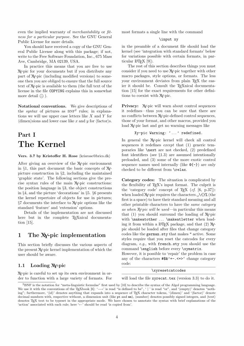
All positions may be written <X,Y > where X is theTEX dimension distance right and Y the distance upfrom the zero position 0 of the XY-picture (0 has co-ordinates <0mm,0mm>, of course). The zero positionof the XY-picture determines the box produced by the\xy. . . \endxy command together with the four pa-rameters Xmin, Xmax, Ymin, and Ymax set such thatall the objects in the picture are ‘contained’ in thefollowing rectangle:
◦0TEX reference point
•ooXmin
//Xmax
��Ymin
OO
Ymax
where the distances follow the “up and right > 0”principle, e.g., the indicated TEX reference point hascoordinates <Xmin,0pt> within the XY-picture. Thezero position does not have to be contained in the pic-ture, but Xmin ≤ Xmax ∧ Ymin ≤ Ymax always holds.The possible positions are described in detail in §3.
When an XY-picture is entered in math mode thenthe reference point becomes the “vcenter” instead,i.e., we use the point <Xmin,-\the\fontdimen22>as reference point.
2.2 Objects
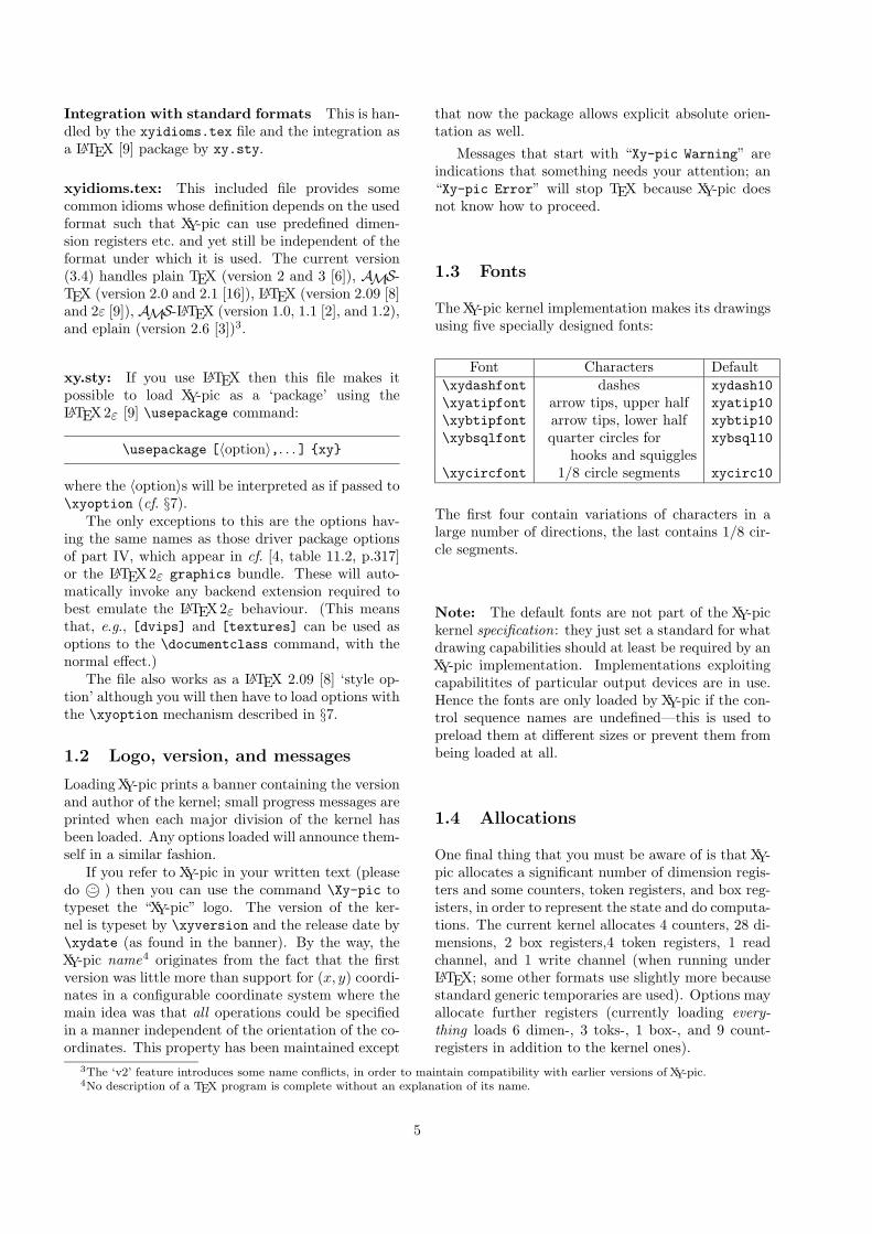
The simplest form of putting things into the pictureis to ‘drop’ an object at a position. An object is likea TEX box except that it has a general Edge aroundits reference point—in particular this has the extents(i.e., it is always contained within) the dimensions L,R, U , and D away from the reference point in eachof the four directions left, right, up, and down. Ob-jects are encoded in TEX boxes using the convention
that the TEX reference point of an object is at its leftedge, thus shifted <−L,0pt> from the center—so aTEX box may be said to be a rectangular object withL = 0pt. Here is an example:
◦L RD
U
TEX reference point•
The object shown has a rectangle edge but others areavailable even though the kernel only supports rect-angle and circle edges. It is also possible to use entireXY-pictures as objects with a rectangle edge, 0 as thereference point, L = −Xmin, R = Xmax, D = −Ymin,and U = Ymax. The commands for objects are de-scribed in §4.
2.3 Connections
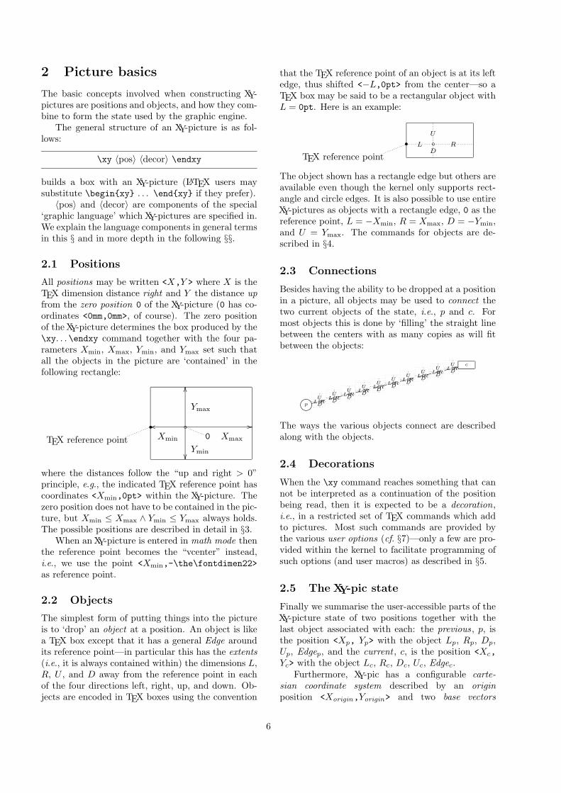
Besides having the ability to be dropped at a positionin a picture, all objects may be used to connect thetwo current objects of the state, i.e., p and c. Formost objects this is done by ‘filling’ the straight linebetween the centers with as many copies as will fitbetween the objects:
p(/).*-+,
cggggggggggggggggg
◦L RD
U
◦L RD
U
◦L RD
U
◦L RD
U
◦L RD
U
◦L RD
U
◦L RD
U
◦L RD
U
◦L RD
U
◦L RD
U
The ways the various objects connect are describedalong with the objects.
2.4 Decorations
When the \xy command reaches something that cannot be interpreted as a continuation of the positionbeing read, then it is expected to be a decoration,i.e., in a restricted set of TEX commands which addto pictures. Most such commands are provided bythe various user options (cf. §7)—only a few are pro-vided within the kernel to facilitate programming ofsuch options (and user macros) as described in §5.
2.5 The XY-pic state
Finally we summarise the user-accessible parts of theXY-picture state of two positions together with thelast object associated with each: the previous, p, isthe position <Xp, Yp> with the object Lp, Rp, Dp,Up, Edgep, and the current , c, is the position <Xc,Yc> with the object Lc, Rc, Dc, Uc, Edgec.
Furthermore, XY-pic has a configurable carte-sian coordinate system described by an originposition <Xorigin,Yorigin> and two base vectors
6
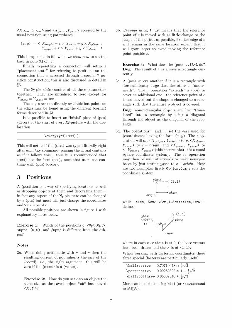
<Xxbase,Yxbase> and <Xybase,Yybase> accessed by theusual notation using parentheses:
(x,y) = < Xorigin + x×Xxbase + y ×Xybase ,Yorigin + x× Yxbase + y × Yybase >
This is explained in full when we show how to set thebase in note 3d of §3.
Finally typesetting a connection will setup a“placement state” for referring to positions on theconnection that is accessed through a special ? po-sition construction; this is also discussed in detail in§3.
The XY-pic state consists of all these parameterstogether. They are initialised to zero except forXxbase = Yybase = 1mm.
The edges are not directly available but points onthe edges may be found using the different 〈corner〉forms described in §3.
It is possible to insert an ‘initial’ piece of 〈pos〉〈decor〉 at the start of every XY-picture with the dec-laration
\everyxy={ 〈text〉 }
This will act as if the 〈text〉 was typed literally rightafter each \xy command, parsing the actual contentsas if it follows this – thus it is recommended that〈text〉 has the form 〈pos〉, such that users can con-tinue with 〈pos〉 〈decor〉.
3 Positions
A 〈pos〉ition is a way of specifying locations as wellas dropping objects at them and decorating them—in fact any aspect of the XY-pic state can be changedby a 〈pos〉 but most will just change the coordinatesand/or shape of c.
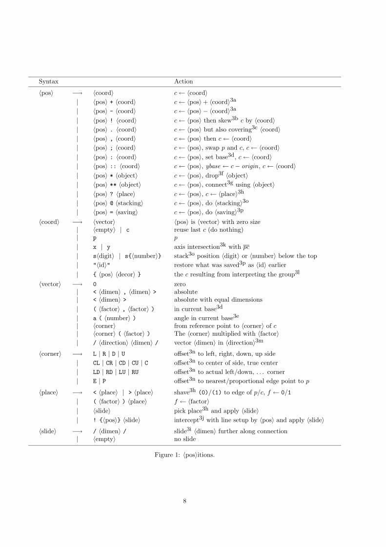
All possible positions are shown in figure 1 withexplanatory notes below.
Exercise 1: Which of the positions 0, <0pt,0pt>,<0pt>, (0,0), and /0pt/ is different from the oth-ers?
Notes
3a. When doing arithmetic with + and - then theresulting current object inherits the size of the〈coord〉, i.e., the right argument—this will bezero if the 〈coord〉 is a 〈vector〉.
Exercise 2: How do you set c to an object thesame size as the saved object "ob" but moved<X,Y >?
3b. Skewing using ! just means that the referencepoint of c is moved with as little change to theshape of the object as possible, i.e., the edge of cwill remain in the same location except that itwill grow larger to avoid moving the referencepoint outside c.
Exercise 3: What does the 〈pos〉 . . . !R-L do?Bug: The result of ! is always a rectangle cur-rently.
3c. A 〈pos〉 covers another if it is a rectangle withsize sufficiently large that the other is “under-neath”. The . operation “extends” a 〈pos〉 tocover an additional one—the reference point of cis not moved but the shape is changed to a rect-angle such that the entire p object is covered.Bug: non-rectangular objects are first “trans-lated” into a rectangle by using a diagonalthrough the object as the diagonal of the rect-angle.
3d. The operations : and :: set the base used for〈coord〉inates having the form (x,y). The : op-eration will set <Xorigin, Yorigin> to p, <Xxbase,Yxbase> to c − origin, and <Xybase, Yybase> to<−Yxbase, Xxbase> (this ensures that it is a usualsquare coordinate system). The :: operationmay then be used afterwards to make nonsqarebases by just setting ybase to c − origin. Hereare two examples: firstly 0;<1cm,0cm>: sets thecoordinate system
◦ //
OO
originxbase
ybase × (1,1)
while <1cm,.5cm>;<2cm,1.5cm>:<1cm,1cm>::defines
◦
??
??
?
__ybasebefore::
���������
??
OO
origin
xbaseybase
× (1,1)
where in each case the ◦ is at 0, the base vectorshave been drawn and the × is at (1,1).When working with cartesian coordinates thesethree special 〈factor〉s are particularly useful:
\halfroottwo 0.70710678 ≈ 12
√2
\partroottwo 0.29289322 ≈ 1− 12
√2
\halfrootthree 0.86602540 ≈ 12
√3
More can be defined using \def (or \newcommandin LATEX).
7
Syntax Action
〈pos〉 −→ 〈coord〉 c← 〈coord〉| 〈pos〉 + 〈coord〉 c← 〈pos〉+ 〈coord〉3a
| 〈pos〉 - 〈coord〉 c← 〈pos〉 − 〈coord〉3a
| 〈pos〉 ! 〈coord〉 c← 〈pos〉 then skew3b c by 〈coord〉| 〈pos〉 . 〈coord〉 c← 〈pos〉 but also covering3c 〈coord〉| 〈pos〉 , 〈coord〉 c← 〈pos〉 then c← 〈coord〉| 〈pos〉 ; 〈coord〉 c← 〈pos〉, swap p and c, c← 〈coord〉| 〈pos〉 : 〈coord〉 c← 〈pos〉, set base3d, c← 〈coord〉| 〈pos〉 :: 〈coord〉 c← 〈pos〉, ybase ← c− origin, c← 〈coord〉| 〈pos〉 * 〈object〉 c← 〈pos〉, drop3f 〈object〉| 〈pos〉 ** 〈object〉 c← 〈pos〉, connect3g using 〈object〉| 〈pos〉 ? 〈place〉 c← 〈pos〉, c← 〈place〉3h
| 〈pos〉 @ 〈stacking〉 c← 〈pos〉, do 〈stacking〉3o
| 〈pos〉 = 〈saving〉 c← 〈pos〉, do 〈saving〉3p
〈coord〉 −→ 〈vector〉 〈pos〉 is 〈vector〉 with zero size| 〈empty〉 | c reuse last c (do nothing)| p p
| x | y axis intersection3k with pc
| s〈digit〉 | s{〈number〉} stack3o position 〈digit〉 or 〈number〉 below the top| "〈id〉" restore what was saved3p as 〈id〉 earlier| { 〈pos〉 〈decor〉 } the c resulting from interpreting the group3l
〈vector〉 −→ 0 zero| < 〈dimen〉 , 〈dimen〉 > absolute| < 〈dimen〉 > absolute with equal dimensions| ( 〈factor〉 , 〈factor〉 ) in current base3d
| a ( 〈number〉 ) angle in current base3e
| 〈corner〉 from reference point to 〈corner〉 of c| 〈corner〉 ( 〈factor〉 ) The 〈corner〉 multiplied with 〈factor〉| / 〈direction〉 〈dimen〉 / vector 〈dimen〉 in 〈direction〉3m
〈corner〉 −→ L | R | D | U offset3n to left, right, down, up side| CL | CR | CD | CU | C offset3n to center of side, true center| LD | RD | LU | RU offset3n to actual left/down, . . . corner| E | P offset3n to nearest/proportional edge point to p
〈place〉 −→ < 〈place〉 | > 〈place〉 shave3h (0)/(1) to edge of p/c, f ← 0/1
| ( 〈factor〉 ) 〈place〉 f ← 〈factor〉| 〈slide〉 pick place3h and apply 〈slide〉| ! {〈pos〉} 〈slide〉 intercept3j with line setup by 〈pos〉 and apply 〈slide〉
〈slide〉 −→ / 〈dimen〉 / slide3i 〈dimen〉 further along connection| 〈empty〉 no slide
Figure 1: 〈pos〉itions.
8
3e. An angle α in XY-pic is the same as the coor-dinate pair ( cosα, sinα) where α must be aninteger interpreted as a number of degrees. Thusthe 〈vector〉 a(0) is the same as (1,0) and a(90)as (0,1), etc.
3f. To drop an 〈object〉 at c with * means to actu-ally physically typeset it in the picture with ref-erence position at c—how this is done dependson the 〈object〉 in question and is described indetail in §4. The intuition with a drop is that ittypesets something at <Xc,Yc> and sets the edgeof c accordingly.
3g. The connect operation ** will first compute anumber of internal parameters describing the di-rection from p to c and then typesets a connectionfilled with copies of the 〈object〉 as illustratedin §2.3. The exact details of the connection de-pend on the actual 〈object〉 and are described ingeneral in §4. The intuition with a connectionis that it typesets something connecting p and cand sets the ? 〈pos〉 operator up accordingly.
3h. Using ? will “pick a place” along the most recentconnection typeset with **. What exactly thismeans is determined by the object that was usedfor the connection and by the modifiers describedin general terms here.
The “shave” modifiers in a 〈place〉, < and >,change the default 〈factor〉, f , and how it is used,by ‘moving’ the positions that correspond to (0)and (1) (respectively): These are initially setequal to p and c, but shaving will move themto the point on the edge of p and c where theconnection “leaves/enters” them, and change thedefault f as indicated. When one end has alreadybeen shaved thus then subsequent shaves will cor-respond to sliding the appropriate position(s) aTEX \jot (usually equal to 3pt) further towardsthe other end of the connection (and past it). Fi-nally the pick action will pick the position locatedthe fraction f of the way from (0) to (1) wheref = 0.5 if it was not set (by <, >, or explicitly).
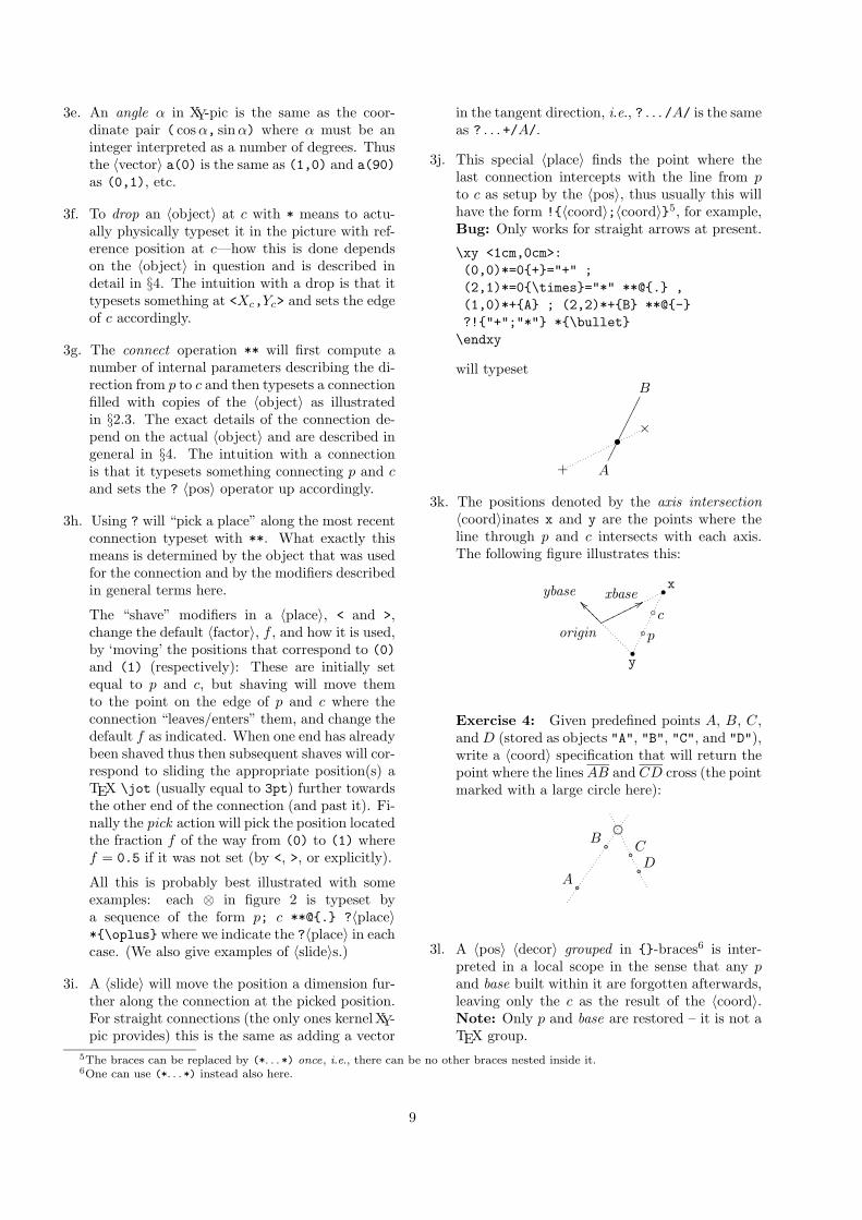
All this is probably best illustrated with someexamples: each ⊗ in figure 2 is typeset bya sequence of the form p; c **@{.} ?〈place〉*{\oplus} where we indicate the ?〈place〉 in eachcase. (We also give examples of 〈slide〉s.)
3i. A 〈slide〉 will move the position a dimension fur-ther along the connection at the picked position.For straight connections (the only ones kernel XY-pic provides) this is the same as adding a vector
in the tangent direction, i.e., ? . . . /A/ is the sameas ? . . . +/A/.
3j. This special 〈place〉 finds the point where thelast connection intercepts with the line from pto c as setup by the 〈pos〉, thus usually this willhave the form !{〈coord〉;〈coord〉}5, for example,Bug: Only works for straight arrows at present.
\xy <1cm,0cm>:(0,0)*=0{+}="+" ;(2,1)*=0{\times}="*" **@{.} ,(1,0)*+{A} ; (2,2)*+{B} **@{-}?!{"+";"*"} *{\bullet}
\endxy
will typeset
+
×
A
B����������
•
3k. The positions denoted by the axis intersection〈coord〉inates x and y are the points where theline through p and c intersects with each axis.The following figure illustrates this:
origin
xbaseooooooo
77ybase ?????__
◦p
◦c
x•
y•
Exercise 4: Given predefined points A, B, C,and D (stored as objects "A", "B", "C", and "D"),write a 〈coord〉 specification that will return thepoint where the linesAB and CD cross (the pointmarked with a large circle here):
��������A
��������B �������� C�������� D��������
3l. A 〈pos〉 〈decor〉 grouped in {}-braces6 is inter-preted in a local scope in the sense that any pand base built within it are forgotten afterwards,leaving only the c as the result of the 〈coord〉.Note: Only p and base are restored – it is not aTEX group.
5The braces can be replaced by (*. . . *) once, i.e., there can be no other braces nested inside it.6One can use (*. . . *) instead also here.
9
GFED@ABC76540123p is circular:
c is asquaretext!
RRRRRRRRRRRRRRRRRRRRRRRRRRR⊕
?(0)
rrrrrr
99
⊕
?(1)
rrrrrr
99
⊕
?
rrrrrr
99
⊕
?(.7)
rrrrrr
99
⊕
?<>(.5)��⊕
?<>(.2)(.5)
rrrrrryy
⊕
?<
rrrrrryy⊕
?<<<
rrrrrr
99⊕
?<<</1cm/
rrrrrr
99⊕
?<(0)��
⊕
?>
rrrrrryy⊕
?>>>>��
⊕
?<>(.7)
rrrrrryy⊕
?>(.7)��
Figure 2: Example 〈place〉s
Exercise 5: What effect is achieved by usingthe 〈coord〉inate “{;}”?
3m. The vector /Z/, where Z is a 〈dimen〉sion, is thesame as the vector <Z cosα,Z sinα> where α isthe angle of the last direction set by a connec-tion (i.e., with **) or subsequent placement (?)position.
It is possible to give a 〈direction〉 as described inthe next section (figure 3, note 4l in particular)that will then be used to set the value of α. It isalso possible to omit the 〈dimen〉 in which caseit is set to a default value of .5pc.
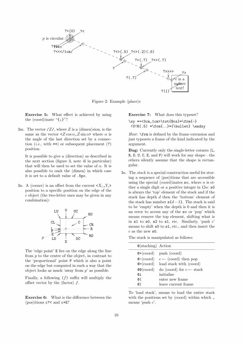
3n. A 〈corner〉 is an offset from the current <Xc,Yc>position to a specific position on the edge of thec object (the two-letter ones may be given in anycombination):
cL // Roo
D
OO
U
��
LDyyy<<
RDVVVkk
LU111��
RUrrryy
CL OOO '' CRdddrr
DC
EEEbb
UC
��
Coooww
Pddd 22
pE
lll66
The ‘edge point’ E lies on the edge along the linefrom p to the centre of the object, in contrast tothe ‘proportional’ point P which is also a pointon the edge but computed in such a way that theobject looks as much ‘away from p’ as possible.
Finally, a following (f) suffix will multiply theoffset vector by the 〈factor〉 f .
Exercise 6: What is the difference between the〈pos〉itions c?< and c+E?
Exercise 7: What does this typeset?
\xy *=<3cm,1cm>\txt{Box}*\frm{-}!U!R(.5) *\frm{..}*{\bullet} \endxy
Hint : \frm is defined by the frame extension andjust typesets a frame of the kind indicated by theargument.
Bug: Currently only the single-letter corners (L,R, D, U, C, E, and P) will work for any shape—theothers silently assume that the shape is rectan-gular.
3o. The stack is a special construction useful for stor-ing a sequence of 〈pos〉itions that are accessibleusing the special 〈coord〉inates sn, where n is ei-ther a single digit or a positive integer in {}s: s0is always the ‘top’ element of the stack and if thestack has depth d then the ‘bottom’ element ofthe stack has number s{d−1}. The stack is saidto be ‘empty’ when the depth is 0 and then it isan error to access any of the sn or ‘pop’ whichmeans remove the top element, shifting what isin s1 to s0, s2 to s1, etc. Similarly, ‘push c’means to shift s0 to s1, etc., and then insert thec as the new s0.
The stack is manipulated as follows:
@〈stacking〉 Action
@+〈coord〉 push 〈coord〉@-〈coord〉 c← 〈coord〉 then pop@=〈coord〉 load stack with 〈coord〉@@〈coord〉 do 〈coord〉 for c← stack@i initialise@( enter new frame@) leave current frame
To ‘load stack’, means to load the entire stackwith the positions set by 〈coord〉 within which ,means ‘push c’.
10
To ‘do 〈coord〉 for all stack elements’ means toset c to each element of the stack in turn, fromthe bottom and up, and for each interpret the〈coord〉. Thus the first interpretation has c setto the bottom element of the stack and the lasthas c set to s0. If the stack is empty, the 〈coord〉is not interpreted at all.
These two operations can be combined to repeata particular 〈coord〉 for several points, like this:
\xy@={(0,-10),(10,3),(20,-5)} @@{*{P}}
\endxy
will typeset
P
P
P
Finally, the stack can be forcibly cleared using@i, however, this is rarely needed because of @(,which saves the stack as it is, and then clears it,such when it has been used (and is empty), and@) is issued, then it is restored as it was at thetime of the @(.
Exercise 8: How would you change the exam-ple above to connect the points as shown below?
gggggggggggg
����������
EEEEEEEE
3p. It is possible to define new 〈coord〉inates on theform "〈id〉" by saving the current c using the. . . ="〈id〉" 〈pos〉ition form. Subsequent uses of"〈id〉" will then reestablish the c at the time ofthe saving.
Using a "〈id〉" that was never defined is an error,however, saving into a name that was previouslydefined just replaces the definition without warn-ing, i.e., "〈id〉" always refers to the last thingsaved with that 〈id〉.However, many other things can be ‘saved’: ingeneral @〈saving〉 has either of the forms
@:"〈id〉" "〈id〉" restores currentbase
@〈coord〉"〈id〉" "〈id〉" reinterprets 〈coord〉@@"〈id〉" @="〈id〉" reloads this stack
The first form defines "〈id〉" to be a macro thatrestores the current base.
The second does not depend on the state at thetime of definition at all; it is a macro definition.
You can pass parameters to such a macro by let-ting it use coordinates named "1", "2", etc., andthen use ="1", ="2", etc., just before every useof it to set the actual values of these. Note: it isnot possible to use a 〈coord〉 of the form "〈id〉"directly: write it as {"〈id〉"}.
Exercise 9: Write a macro "dbl" to double thesize of the current c object, e.g., changing it fromthe dotted to the dashed outline in this figure:
+
_ _ _ _ _ _ _ _ _������
������
_ _ _ _ _ _ _ _ _
The final form defines a special kind of macrothat should only be used after the @= stack oper-ation: the entire current stack is saved such thatthe stack operation @="〈id〉" will reload it.
Note: There is no distinction between the ‘namespaces’ of 〈id〉s used for saved coordinates andother things.
4 Objects
Objects are the entities that are manipulated withthe * and ** 〈pos〉 operations above to actually getsome output in XY-pictures. As for 〈pos〉itions theoperations are interpreted strictly from left to right,however, the actual object is built before all the〈modifier〉s take effect. The syntax of objects is givenin figure 3 with references to the notes below. Re-mark: It is never allowed to include braces {} inside〈modifier〉s! In case you wish to do something thatrequires {. . . } then check in this manual whether youcan use (*. . . *) instead. If not then you will have touse a different construction!
Notes
4a. An 〈object〉 is built using \objectbox {〈text〉}.\objectbox is initially defined as
\def\objectbox#1{%\hbox{$\objectstyle{#1}$}}
\let\objectstyle=\displaystyle
but may be redefined by options or the user.The 〈text〉 should thus be in the mode requiredby the \objectbox command—with the default\objectbox shown above it should be in mathmode.
11
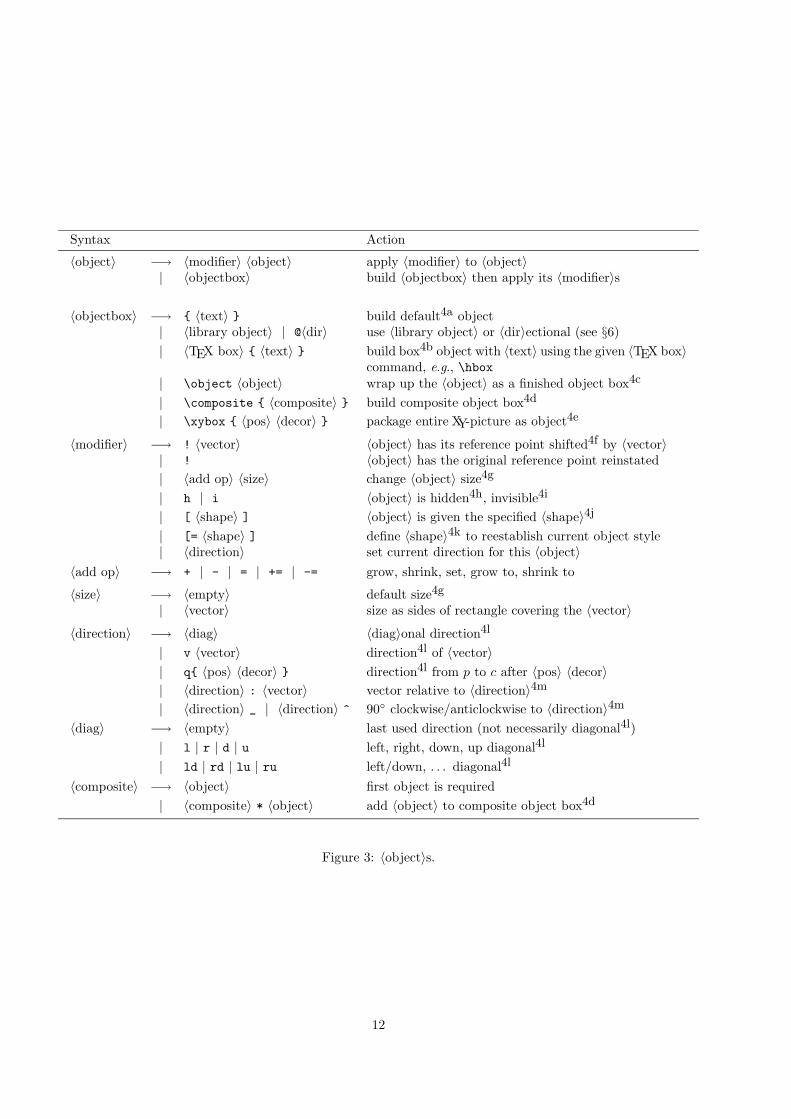
Syntax Action
〈object〉 −→ 〈modifier〉 〈object〉 apply 〈modifier〉 to 〈object〉| 〈objectbox〉 build 〈objectbox〉 then apply its 〈modifier〉s
〈objectbox〉 −→ { 〈text〉 } build default4a object| 〈library object〉 | @〈dir〉 use 〈library object〉 or 〈dir〉ectional (see §6)| 〈TEX box〉 { 〈text〉 } build box4b object with 〈text〉 using the given 〈TEX box〉
command, e.g., \hbox| \object 〈object〉 wrap up the 〈object〉 as a finished object box4c
| \composite { 〈composite〉 } build composite object box4d
| \xybox { 〈pos〉 〈decor〉 } package entire XY-picture as object4e
〈modifier〉 −→ ! 〈vector〉 〈object〉 has its reference point shifted4f by 〈vector〉| ! 〈object〉 has the original reference point reinstated| 〈add op〉 〈size〉 change 〈object〉 size4g
| h | i 〈object〉 is hidden4h, invisible4i
| [ 〈shape〉 ] 〈object〉 is given the specified 〈shape〉4j
| [= 〈shape〉 ] define 〈shape〉4k to reestablish current object style| 〈direction〉 set current direction for this 〈object〉
〈add op〉 −→ + | - | = | += | -= grow, shrink, set, grow to, shrink to
〈size〉 −→ 〈empty〉 default size4g
| 〈vector〉 size as sides of rectangle covering the 〈vector〉
〈direction〉 −→ 〈diag〉 〈diag〉onal direction4l
| v 〈vector〉 direction4l of 〈vector〉| q{ 〈pos〉 〈decor〉 } direction4l from p to c after 〈pos〉 〈decor〉| 〈direction〉 : 〈vector〉 vector relative to 〈direction〉4m
| 〈direction〉 _ | 〈direction〉 ^ 90◦ clockwise/anticlockwise to 〈direction〉4m
〈diag〉 −→ 〈empty〉 last used direction (not necessarily diagonal4l)| l | r | d | u left, right, down, up diagonal4l
| ld | rd | lu | ru left/down, . . . diagonal4l
〈composite〉 −→ 〈object〉 first object is required| 〈composite〉 * 〈object〉 add 〈object〉 to composite object box4d
Figure 3: 〈object〉s.
12
4b. An 〈object〉 built from a TEX box with dimen-sions w × (h + d) will have Lc = Rc = w/2,Uc = Dc = (h + d)/2, thus initially be equippedwith the adjustment !C (see note 4f). In partic-ular: in order to get the reference point on the(center of) the base line of the original 〈TEX box〉then you should use the 〈modifier〉 !; to get thereference point identical to the TEX referencepoint use the modifier !!L.
TEXnical remark: Any macro that expands tosomething that starts with a 〈box〉 may be usedas a 〈TEX box〉 here.
4c. Takes an object and constructs it, building a box;it is then processed according to the preceedingmodifiers. This form makes it possible to useany 〈object〉 as a TEX box (even outside of XY-pictures) because a finished object is always alsoa box.
4d. Several 〈object〉s can be combined into a singleobject using the special command \compositewith a list of the desired objects separated with*s as the argument. The resulting box (and ob-ject) is the least rectangle enclosing all the in-cluded objects.
4e. Take an entire XY-picture and wrap it up as abox as described in §2.1. Makes nesting of XY-pictures possible: the inner picture will have itsown zero point which will be its reference pointin the outer picture when it is placed there.
4f. An object is shifted a 〈vector〉 by moving thepoint inside it which will be used as the refer-ence point. This effectively pushes the object thesame amount in the opposite direction.
Exercise 10: What is the difference betweenthe 〈pos〉itions 0*{a}!DR and 0*!DR{a}?
4g. A 〈size〉 is a pair <W,H> of the width and heightof a rectangle. When given as a 〈vector〉 theseare just the vector coordinates, i.e., the 〈vector〉starts in the lower left corner and ends in the up-per right corner. The possible 〈add op〉erationsthat can be performed are described in the fol-lowing table.
〈add op〉 description+ grow- shrink= set to+= grow to at least-= shrink to at most
In each case the 〈vector〉 may be omitted whichinvokes the “default size” for the particular 〈add
op〉:
〈add op〉 default+ +<2× objectmargin>- -<2× objectmargin>= =<objectwidth,objectheight>+= +=<max(Lc +Rc, Dc + Uc)>-= -=<min(Lc +Rc, Dc + Uc)>
The defaults for the first three are set with thecommands
\objectmargin 〈add op〉 {〈dimen〉}\objectwidth 〈add op〉 {〈dimen〉}\objectheight 〈add op〉 {〈dimen〉}
where 〈add op〉 is interpreted in the same way asabove.
The defaults for +=/-= are such that the result-ing object will be the smallest containing/largestcontained square.
Exercise 11: How are the objects typeset bythe 〈pos〉itions “*+UR{\sum}” and “*+DL{\sum}”enlarged?
Bug: Currently changing the size of a circularobject is buggy—it is changed as if it is a rect-angle and then the change to the R parameteraffects the circle. This should be fixed probablyby a generalisation of the o shape to be ovals orellipses with horizontal/vertical axes.
4h. A hidden object will be typeset but hidden fromXY-pic in that it won’t affect the size of the entirepicture as discussed in §2.1.
4i. An invisible object will be treated completelynormal except that it won’t be typeset, i.e., XY-pic will behave as if it was.
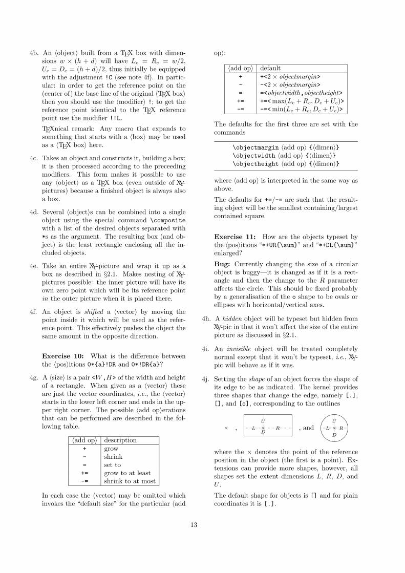
4j. Setting the shape of an object forces the shape ofits edge to be as indicated. The kernel providesthree shapes that change the edge, namely [.],[], and [o], corresponding to the outlines
× , ×L RD
U
, and ×gafbecdL R
D
U
where the × denotes the point of the referenceposition in the object (the first is a point). Ex-tensions can provide more shapes, however, allshapes set the extent dimensions L, R, D, andU .
The default shape for objects is [] and for plaincoordinates it is [.].
13
Furthermore the 〈shape〉s [r], [l], [u], and [d],are defined for convenience to adjust the object tothe indicated side by setting the reference pointsuch that the reference point is the same dis-tance from the opposite of the indicated edgeand the two neighbour edges but never closerto the indicated side than the opposite edge,e.g., the object [r]\hbox{Wide text} has refer-ence point at the × in Wide text× but the object[d]\hbox{Wide text} has reference point at the× in Wide text× . Finally, [c] puts the referencepoint at the center.
Note: Extensions can add new 〈shape〉 object〈modifier〉s which are then called 〈style〉s. Thesewill always be either of the form [〈keyword〉] or[〈character〉 〈argument〉]. Some of these 〈style〉sdo other things than set the edge of the object.
4k. While typesetting an object, some of the prop-erties are considered part of the ‘current objectstyle’. Initially this means nothing but some ofthe 〈style〉s defined by extensions have this sta-tus, e.g., colours [red], [blue] say, using thexycolor extension, or varying the width of linesusing xyline. Such styles are processed left-to-right ; for example,
*[red][green][=NEW][blue]{A}
will typeset a blue A and define [NEW] to set thecolour to green (all provided that xycolor hasbeen loaded, of course).
Saving styles: Once specified for an 〈object〉,the collection of 〈style〉s can be assigned a name,using [=〈word〉]. Then [〈word〉] becomes a new〈style〉, suitable for use with the same or other〈objects〉s. Use a single 〈word〉 built from ordi-nary letters. If [〈word〉] already had meaningthe new definition will still be imposed, but thefollowing type of warning will be issued:
Xy-pic Warning: Redefining style [〈word〉]
The latter warning will appear if the definitionoccurs within an \xymatrix. This is perfectlynormal, being a consequence of the way that thematrix code is handled. Similarly the messagemay appear several times if the style definition ismade within an \ar.
The following illustrates how to avoid these mes-sages by defining the style without typesettinganything.
\setbox0=\hbox{%\xy\drop[OrangeRed][=A]{}\endxy}
Note 1: The current colour is regarded as partof the style for this purpose.
Note 2: Such namings are global in scope. Theyare intended to allow a consistent style to be eas-ily maintained between various pictures and dia-grams within the same document.
If the same 〈style〉 is intended for several〈object〉s occurring in succession, the [|*]〈modifier〉 can be used on the later 〈object〉s.This only works when [|*] precedes any other〈style〉 modifiers; it is local in scope, recoveringthe last 〈style〉s used at the same level of TEXgrouping.
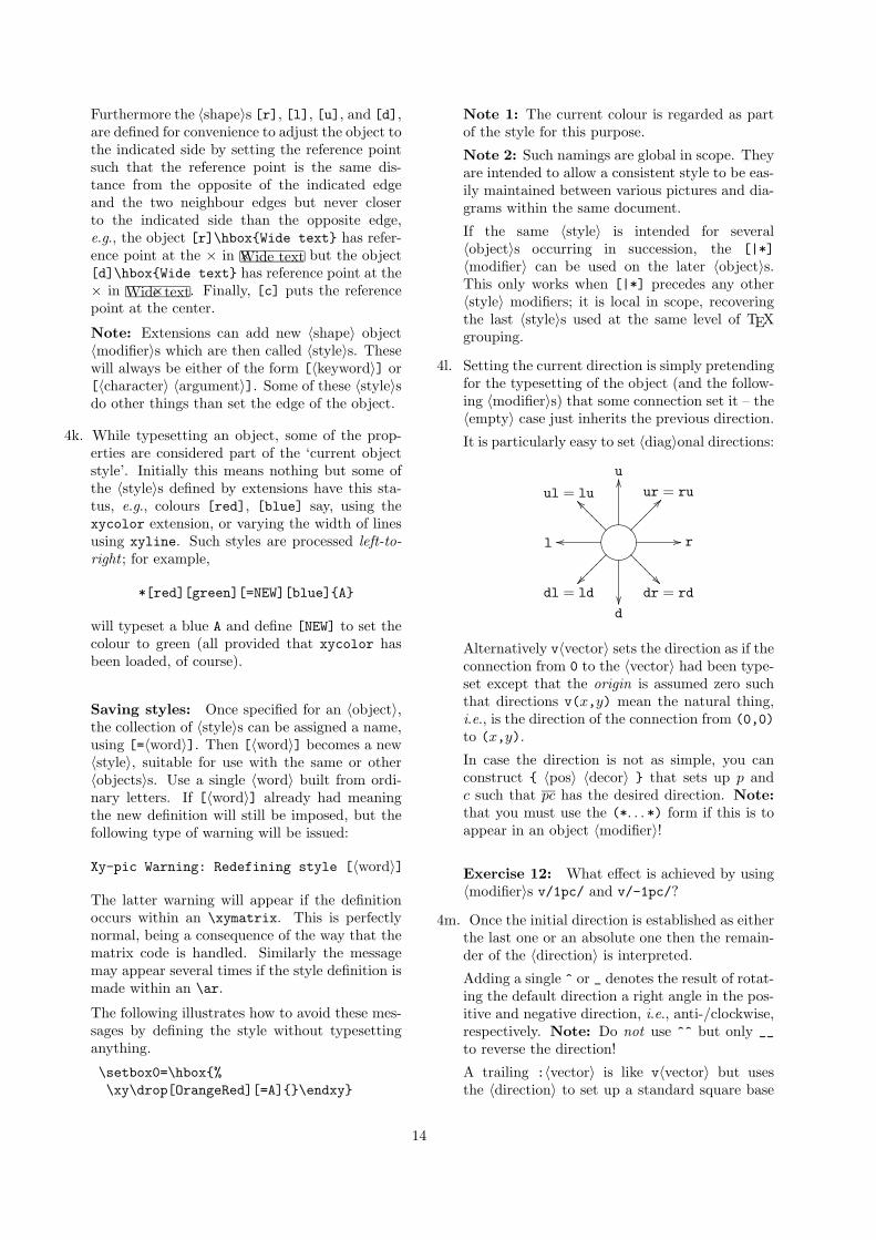
4l. Setting the current direction is simply pretendingfor the typesetting of the object (and the follow-ing 〈modifier〉s) that some connection set it – the〈empty〉 case just inherits the previous direction.
It is particularly easy to set 〈diag〉onal directions:
HOINJMKL
dl = ld������
��
d�� dr = rd
??????
��
r//
ur = ru������
??
uOOul = lu??????
__
l oo
Alternatively v〈vector〉 sets the direction as if theconnection from 0 to the 〈vector〉 had been type-set except that the origin is assumed zero suchthat directions v(x,y) mean the natural thing,i.e., is the direction of the connection from (0,0)to (x,y).
In case the direction is not as simple, you canconstruct { 〈pos〉 〈decor〉 } that sets up p andc such that pc has the desired direction. Note:that you must use the (*. . . *) form if this is toappear in an object 〈modifier〉!
Exercise 12: What effect is achieved by using〈modifier〉s v/1pc/ and v/-1pc/?
4m. Once the initial direction is established as eitherthe last one or an absolute one then the remain-der of the 〈direction〉 is interpreted.
Adding a single ^ or _ denotes the result of rotat-ing the default direction a right angle in the pos-itive and negative direction, i.e., anti-/clockwise,respectively. Note: Do not use ^^ but only __to reverse the direction!
A trailing :〈vector〉 is like v〈vector〉 but usesthe 〈direction〉 to set up a standard square base
14
such that :(0,1) and :(0,-1) mean the same as:a(90) and :a(-90) and as ^ and _, respectively.
Exercise 13: What effect is achieved by using〈modifier〉s v/1pc/:(1,0) and v/-1pc/__?
5 Decorations
〈Decor〉ations are actual TEX macros that decoratethe current picture in manners that depend on thestate. They are allowed after the 〈pos〉ition either ofthe outer \xy. . . \endxy or inside {. . . }. The possi-bilities are given in figure 4 with notes below.
Most options add to the available 〈decor〉, inparticular the v2 option loads many more since XY-pic versions prior to 2.7 provided most features as〈decor〉.
Notes
5a. Saving and restoring allows ‘excursions’ wherelots of things are added to the picture withoutaffecting the resulting XY-pic state, i.e., c, p, andbase, and without requiring matching {}s. Theindependence of {} is particularly useful in con-junction with the \afterPOS command, for ex-ample, the definition
\def\ToPOS{\save\afterPOS{%\POS**{}?>*@2{>}**@{-}\restore};p,}
will cause the code \ToPOS〈pos〉 to construct adouble-shafted arrow from the current object tothe 〈pos〉 (computed relative to it) such that \xy*{A} \ToPOS +<10mm,2mm>\endxy will typesetthe pictureA
.6eeeee .
Note: Saving this way in fact uses the samestate as the {} ‘grouping’, so the code p1,{p2\save}, . . . {\restore} will have c = p1
both at the . . . and at the end!
5b. One very tempting kind of TEX commands toperform as 〈decor〉 is arithmetic operations onthe XY-pic state. This will work in simple XY-pictures as described here but be warned: it isnot portable because all XY-pic execution is indi-rect, and this is used by several options in non-trivial ways. Check the TEX-nical documenta-tion [15] for details about this!
Macros that expand to 〈decor〉 will always do thesame, though.
5c. \xyecho will turn on echoing of all interpretedXY-pic 〈pos〉 characters. Bug: Not completelyimplemented yet. \xyverbose will switch on a
tracing of all XY-pic commands executed, withline numbers. \xytracing traces even more: theentire XY-pic state is printed after each modifica-tion. \xyquiet restores default quiet operation.
5d. Ignoring means that the 〈pos〉 〈decor〉 is stillparsed the usual way but nothing is typeset andthe XY-pic state is not changed.
5e. It is possible to save an intermediate form of com-mands that generate parts of an XY-picture toa file such that subsequent typesetting of thoseparts is significantly faster: this is called com-piling . The produced file contains code to checkthat the compiled code still corresponds to thesame 〈pos〉〈decor〉 as well as efficient XY-code toredo it; if the 〈pos〉〈decor〉 has changed then thecompilation is redone.
There are two ways to use this. The direct isto invent a 〈name〉 for each diagram and thenembrace it in \xycompileto{〈name〉}|{. . . } –this dumps the compiled code into the file〈name〉.xyc.
When many diagrams are compiled then itis easier to add \xycompile{. . . } around the〈pos〉〈decor〉 to be compiled. This will assignfile names numbered consecutively with a 〈prefix〉which is initially the expansion of \jobname- butmay be set with
\CompilePrefix{〈prefix〉}
This has the disadvantage, however, that if addi-tional compiled XY-pictures are inserted then allsubsequent pictures will have to be recompiled.One particular situation is provided, though:when used within constructions that typeset theircontents more than once (such as most AMS-LATEX equation constructs) then the declaration
\CompileFixPoint{〈id〉}
can be used inside the environment to fix thecounter to have the same value at every passage.
Finally, when many ‘administrative typesettingruns’ are needed, e.g., readjusting LATEX crossreferences and such, then it may be an advan-tage to not typeset any XY-pictures at all duringthe intermediate runs. This is supported by thefollowing declarations which for each compilationcreates a special file with the extension .xyd con-taining just the size of the picture:
\MakeOutlines\OnlyOutlines\ShowOutlines
15
Syntax Action
〈decor〉 −→ 〈command〉 〈decor〉 either there is a command. . .| 〈empty〉 . . . or there isn’t.
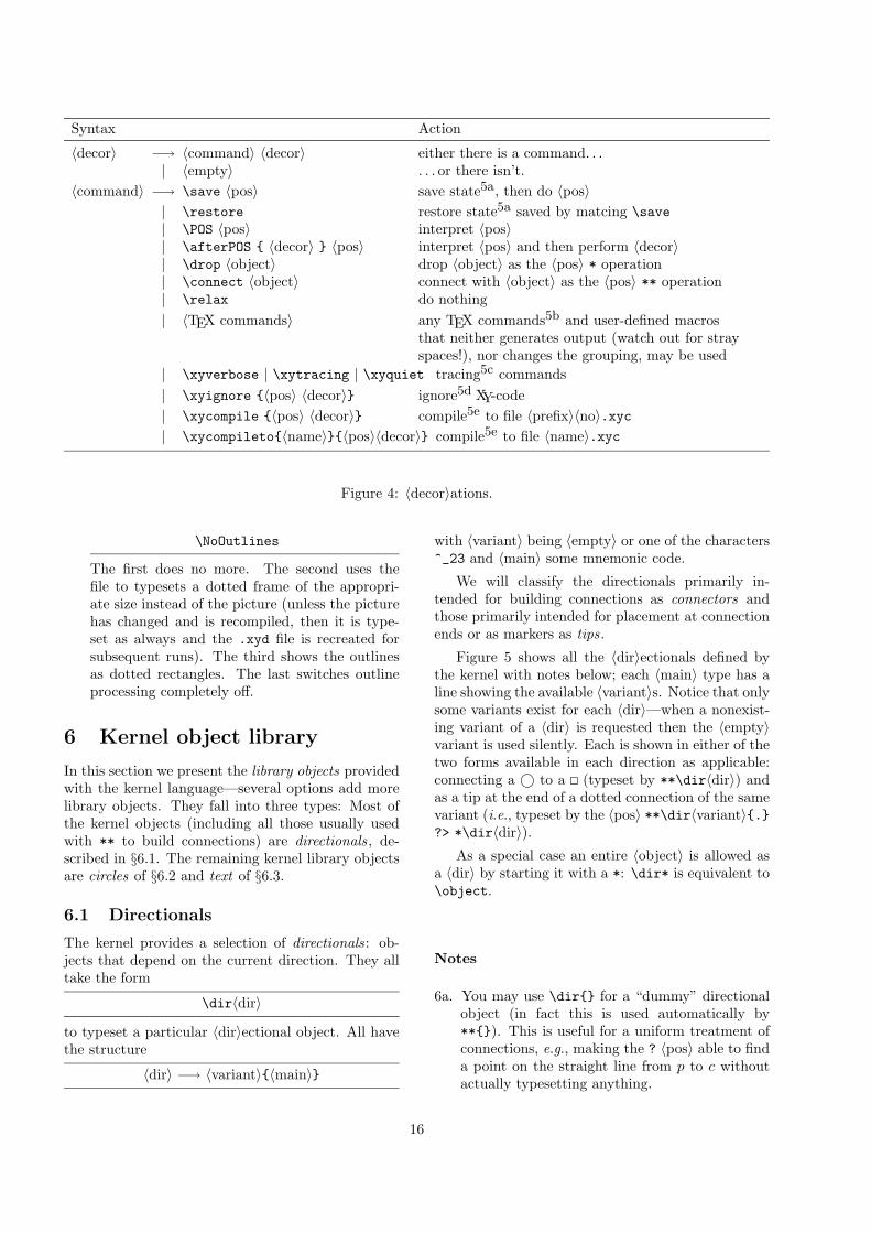
〈command〉 −→ \save 〈pos〉 save state5a, then do 〈pos〉| \restore restore state5a saved by matcing \save| \POS 〈pos〉 interpret 〈pos〉| \afterPOS { 〈decor〉 } 〈pos〉 interpret 〈pos〉 and then perform 〈decor〉| \drop 〈object〉 drop 〈object〉 as the 〈pos〉 * operation| \connect 〈object〉 connect with 〈object〉 as the 〈pos〉 ** operation| \relax do nothing| 〈TEX commands〉 any TEX commands5b and user-defined macros
that neither generates output (watch out for strayspaces!), nor changes the grouping, may be used
| \xyverbose | \xytracing | \xyquiet tracing5c commands| \xyignore {〈pos〉 〈decor〉} ignore5d XY-code| \xycompile {〈pos〉 〈decor〉} compile5e to file 〈prefix〉〈no〉.xyc| \xycompileto{〈name〉}{〈pos〉〈decor〉} compile5e to file 〈name〉.xyc
Figure 4: 〈decor〉ations.
\NoOutlines
The first does no more. The second uses thefile to typesets a dotted frame of the appropri-ate size instead of the picture (unless the picturehas changed and is recompiled, then it is type-set as always and the .xyd file is recreated forsubsequent runs). The third shows the outlinesas dotted rectangles. The last switches outlineprocessing completely off.
6 Kernel object library
In this section we present the library objects providedwith the kernel language—several options add morelibrary objects. They fall into three types: Most ofthe kernel objects (including all those usually usedwith ** to build connections) are directionals, de-scribed in §6.1. The remaining kernel library objectsare circles of §6.2 and text of §6.3.
6.1 Directionals
The kernel provides a selection of directionals: ob-jects that depend on the current direction. They alltake the form
\dir〈dir〉
to typeset a particular 〈dir〉ectional object. All havethe structure
〈dir〉 −→ 〈variant〉{〈main〉}
with 〈variant〉 being 〈empty〉 or one of the characters^_23 and 〈main〉 some mnemonic code.
We will classify the directionals primarily in-tended for building connections as connectors andthose primarily intended for placement at connectionends or as markers as tips.
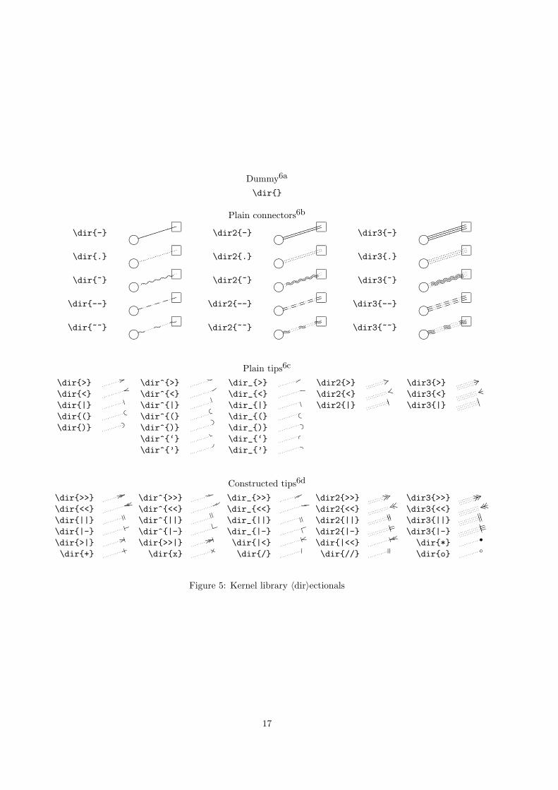
Figure 5 shows all the 〈dir〉ectionals defined bythe kernel with notes below; each 〈main〉 type has aline showing the available 〈variant〉s. Notice that onlysome variants exist for each 〈dir〉—when a nonexist-ing variant of a 〈dir〉 is requested then the 〈empty〉variant is used silently. Each is shown in either of thetwo forms available in each direction as applicable:connecting a © to a (typeset by **\dir〈dir〉) andas a tip at the end of a dotted connection of the samevariant (i.e., typeset by the 〈pos〉 **\dir〈variant〉{.}?> *\dir〈dir〉).
As a special case an entire 〈object〉 is allowed asa 〈dir〉 by starting it with a *: \dir* is equivalent to\object.
Notes
6a. You may use \dir{} for a “dummy” directionalobject (in fact this is used automatically by**{}). This is useful for a uniform treatment ofconnections, e.g., making the ? 〈pos〉 able to finda point on the straight line from p to c withoutactually typesetting anything.
16
Dummy6a
\dir{}
Plain connectors6b
\dir{-} '!&"%#$iiiiiiiii \dir2{-} '!&"%#$
iiiiiiiiiiiiiiiiii \dir3{-} '!&"%#$
iiiiiiiiiiiiiiiiii
iiiiiiiii
\dir{.} '!&"%#$ \dir2{.} '!&"%#$ \dir3{.} '!&"%#$\dir{~} '!&"%#$ 4t4t4t4t4t \dir2{~} '!&"%#$
4t4t4t4t4t4t4t4t4t4t \dir3{~} '!&"%#$
4t4t4t4t4t4t4t4t4t4t
4t4t4t4t4t
\dir{--} '!&"%#$iiiii \dir2{--} '!&"%#$
iiiiiiiiii \dir3{--} '!&"%#$
iiiiiiiiii
iiiii
\dir{~~} '!&"%#$4t
4t4t \dir2{~~} '!&"%#$
4t4t
4t4t
4t4t \dir3{~~} '!&"%#$
4t4t
4t4t
4t4t
4t4t
4t
Plain tips6c
\dir{>}44
\dir^{>}4
\dir_{>}4
\dir2{>} 08 \dir3{>} i/:
\dir{<}tt
\dir^{<}t
\dir_{<}t
\dir2{<} px \dir3{<} ioz
\dir{|})
\dir^{|})
\dir_{|})
\dir2{|}))
\dir3{|}))
\dir{(}' �
\dir^{(}' �
\dir_{(}�'
\dir{)}gG \dir^{)}
G g\dir_{)} gG
\dir^{‘}'
\dir_{‘}�
\dir^{’}G
\dir_{’} g
Constructed tips6d
\dir{>>} 44 44 \dir^{>>} 4 4 \dir_{>>} 4 4 \dir2{>>} 08 08 \dir3{>>} i/:i/:
\dir{<<}tttt
\dir^{<<}tt
\dir_{<<}tt
\dir2{<<}pxpx \dir3{<<}
iozioz
\dir{||}) )
\dir^{||}) )
\dir_{||}) )
\dir2{||}) )) )
\dir3{||}) )) )
\dir{|-})i
\dir^{|-})i
\dir_{|-})i
\dir2{|-})i)i \dir3{|-}
)i)i)i
\dir{>|})44
\dir{>>|})44 44 \dir{|<}
)tt\dir{|<<}
) tttt\dir{*} •
\dir{+})i
\dir{x}N� \dir{/}
�\dir{//}
� �\dir{o} ◦
Figure 5: Kernel library 〈dir〉ectionals
17
6b. The plain connectors group contains basic direc-tionals that lend themself to simple connections.
By default XY-pic will typeset horizontal and ver-tical \dir{-} connections using TEX rules. Un-fortunately rules is the feature of the DVI formatmost commonly handled wrong by DVI drivers.Therefore XY-pic provides the 〈decor〉ations
\NoRules\UseRules
that will switch the use of such off and on.
As can be seen by the last two columns, these(and most of the other connectors) also ex-ist in double and triple versions with a 2or a 3 prepended to the name. For conve-nience \dir{=} and \dir{:} are synonyms for\dir2{-} and \dir2{.}, respectively; similarly\dir{==} is a synonym for \dir2{--}.
6c. The group of plain tips contains basic objectsthat are useful as markers and arrowheads mak-ing connections, so each is shown at the end of adotted connection of the appropriate kind.
They may also be used as connectors and willbuild dotted connections. e.g., **@{>} typesets
444444444444
Exercise 14: Typeset the following two +s anda tilted square:
++o
//o
Hint : the dash created by \dir{-} has the length5pt (here).
6d. These tips are combinations of the plain tipsprovided for convenience (and optimised for ef-ficiency). New ones can be constructed using\composite and by declarations of the form
\newdir 〈dir〉 {〈composite〉}
which defines \dir〈dir〉 as the 〈composite〉 (seenote 4d for the details).
6.2 Circle segments
Circle 〈object〉s are round and typeset a segment ofthe circle centered at the reference point. The syntaxof circles is described in figure 6 with explanationsbelow.
The default is to generate a full circle with thespecified radius, e.g.,
\xy*\cir<4pt>{}\endxy typesets “��������”\xy*{M}*\cir{}\endxy — “M '!&"%#$”
All the other circle segments are subsets of this andhave the shape that the full circle outlines.
Partial circle segments with 〈orient〉ation are thepart of the full circle that starts with a tangent vec-tor in the direction of the first 〈diag〉onal (see note 4l)and ends with a tangent vector in the direction of theother 〈diag〉onal after a clockwise (for _) or anticlock-wise (for ^) turn, e.g.,
\xy*\cir<4pt>{l^r}\endxy typesets “���� ”\xy*\cir<4pt>{l_r}\endxy — “���� ”\xy*\cir<4pt>{dl^u}\endxy — “�����”\xy*\cir<4pt>{dl_u}\endxy — “��� ”\xy*+{M}*\cir{dr_ur}\endxy — “ M8?9:;<”
If the same 〈diag〉 is given twice then nothing is type-set, e.g.,
\xy*\cir<4pt>{u^u}\endxy typesets “ ”
Special care is taken to setup the 〈diag〉onal defaults:
• After ^ the default is the diagonal 90◦ anticlock-wise from the one before the ^.
• After _ the default is the diagonal 90◦ clockwisefrom the one before the _.
The 〈diag〉 before ^ or _ is required for \cir 〈objects〉.
Exercise 15: Typeset the following shaded circlewith radius 5pt: '!&"%#$!"#$!"#$!"#$
6.3 Text
Text in pictures is supported through the 〈object〉construction
\txt 〈width〉 〈style〉 {〈text〉}
that builds an object containing 〈text〉 typeset to〈width〉 using 〈style〉; in 〈text〉 \\ can be used as anexplicit line break; all lines will be centered. 〈style〉should either be a font command or some other stuffto do for each line of the 〈text〉 and 〈width〉 shouldbe either <〈dimen〉> or 〈empty〉.
7 XY-pic options
Note: LATEX 2ε users should also consult the para-graph on “xy.sty” in §1.1.
18
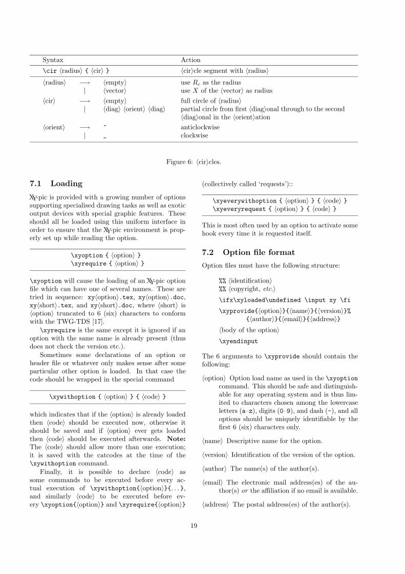
Syntax Action
\cir 〈radius〉 { 〈cir〉 } 〈cir〉cle segment with 〈radius〉
〈radius〉 −→ 〈empty〉 use Rc as the radius| 〈vector〉 use X of the 〈vector〉 as radius
〈cir〉 −→ 〈empty〉 full circle of 〈radius〉| 〈diag〉 〈orient〉 〈diag〉 partial circle from first 〈diag〉onal through to the second
〈diag〉onal in the 〈orient〉ation〈orient〉 −→ ^ anticlockwise
| _ clockwise
Figure 6: 〈cir〉cles.
7.1 Loading
XY-pic is provided with a growing number of optionssupporting specialised drawing tasks as well as exoticoutput devices with special graphic features. Theseshould all be loaded using this uniform interface inorder to ensure that the XY-pic environment is prop-erly set up while reading the option.
\xyoption { 〈option〉 }\xyrequire { 〈option〉 }
\xyoption will cause the loading of an XY-pic optionfile which can have one of several names. These aretried in sequence: xy〈option〉.tex, xy〈option〉.doc,xy〈short〉.tex, and xy〈short〉.doc, where 〈short〉 is〈option〉 truncated to 6 (six) characters to conformwith the TWG-TDS [17].
\xyrequire is the same except it is ignored if anoption with the same name is already present (thusdoes not check the version etc.).
Sometimes some declarations of an option orheader file or whatever only makes sense after someparticular other option is loaded. In that case thecode should be wrapped in the special command
\xywithoption { 〈option〉 } { 〈code〉 }
which indicates that if the 〈option〉 is already loadedthen 〈code〉 should be executed now, otherwise itshould be saved and if 〈option〉 ever gets loadedthen 〈code〉 should be executed afterwards. Note:The 〈code〉 should allow more than one execution;it is saved with the catcodes at the time of the\xywithoption command.
Finally, it is possible to declare 〈code〉 assome commands to be executed before every ac-tual execution of \xywithoption{〈option〉}{. . . },and similarly 〈code〉 to be executed before ev-ery \xyoption{〈option〉} and \xyrequire{〈option〉}
(collectively called ‘requests’)::
\xyeverywithoption { 〈option〉 } { 〈code〉 }\xyeveryrequest { 〈option〉 } { 〈code〉 }
This is most often used by an option to activate somehook every time it is requested itself.
7.2 Option file format
Option files must have the following structure:
%% 〈identification〉%% 〈copyright, etc.〉\ifx\xyloaded\undefined \input xy \fi
\xyprovide{〈option〉}{〈name〉}{〈version〉}%{〈author〉}{〈email〉}{〈address〉}
〈body of the option〉\xyendinput
The 6 arguments to \xyprovide should contain thefollowing:
〈option〉 Option load name as used in the \xyoptioncommand. This should be safe and distinguish-able for any operating system and is thus lim-ited to characters chosen among the lowercaseletters (a–z), digits (0–9), and dash (-), and alloptions should be uniquely identifiable by thefirst 6 (six) characters only.
〈name〉 Descriptive name for the option.
〈version〉 Identification of the version of the option.
〈author〉 The name(s) of the author(s).
〈email〉 The electronic mail address(es) of the au-thor(s) or the affiliation if no email is available.
〈address〉 The postal address(es) of the author(s).
19
This information is used not only to print a nice ban-ner but also to (1) silently skip loading if the sameversion was preloaded and (2) print an error messageif a different version was preloaded.
The ‘dummy’ option described in §22 is a minimaloption using the above features. It uses the specialDOCMODE format to include its own documentation forthis document (like all official XY-pic options) but thisis not a requirement.
7.3 Driver options
The 〈driver〉 options described in part IV require spe-cial attention because each driver can support severalextension options, and it is sometimes desirable tochange 〈driver〉 or even mix the support provided byseveral.7
A 〈driver〉 option is loaded as other options with\xyoption{〈driver〉} (or through LATEX 2ε class orpackage options as described in §1.1). The specialthing about a 〈driver〉 is that loading it simply de-clares the name of it, establishes what extensions itwill support, and selects it temporarily. Thus thespecial capabilities of the driver will only be exploitedin the produced DVI file if some of these extensionsare also loaded and if the driver is still selected whenoutput is produced. Generally, the order in which theoptions are loaded is immaterial. (Known exceptionsaffect only internal processing and are not visible tothe user in terms of language and expected output.)In particular one driver can be preloaded in a formatand a different one used for a particular document.
The following declarations control this:
\UseSingleDriver forces one driver only\MultipleDrivers allows multiple drivers\xyReloadDrivers resets driver information
The first command restores the default behaviour:that ony one 〈driver〉 is allowed, i.e., each loadingof a 〈driver〉 option cancels the previous. The sec-ond allows consecutive loading of drivers such thatwhen loading a 〈driver〉 only the extensions actuallysupported are selected, leaving other extensions sup-ported by previously selected drivers untouched. Be-ware that this can be used to create DVI files thatcannot be processed by any actual DVI driver pro-gram!
The last command is sometimes required to resetthe XY-pic 〈driver〉 information to a sane state, forexample, after having applied one of the other twoin the middle of a document, or when using simpleformats like plain TEX that do not have a clearly dis-tinguished preamble.
As the above suggests it sometimes makes senseto load 〈driver〉s in the actual textual part of a doc-ument, however, it is recommended that only driversalso loaded in the preamble are reloaded later, andthat \xyReloadDrivers is used when there is doubtabout the state of affairs. In case of confusionthe special command \xyShowDrivers will list allthe presently supported and selected driver-extensionpairs to the TEX log.
It is not difficult to add support for additional〈driver〉s; how is described in the TEXnical documen-tation.
Most extensions will print a warning when a capa-bility is used which is not supported by the presentlyloaded 〈driver〉. Such messages are only printed once,however, (for some formats they are repeated at theend). Similarly, when the support of an extensionthat exploits a particular 〈driver〉 is used a warn-ing message will be issued that the DVI file is notportable.
Part II
ExtensionsThis part documents the graphic capabilities addedby each standard extension option. For each is indi-cated the described version number, the author, andhow it is loaded.
Many of these are only fully supported when asuitable driver option (described in part IV) is alsoloaded, however, all added constructions are alwaysaccepted even when not supported.
8 Curve and Spline extension
Vers. 3.7 by Ross Moore 〈[email protected]〉Load as: \xyoption{curve}
This option provides XY-pic with the ability to type-set spline curves by constructing curved connectionsusing arbitrary directional objects and by encirclingobjects similarly. Warning : Using curves can bequite a strain on TEX’s memory; you should there-fore limit the length and number of curves used on asingle page. Memory use is less when combined witha backend capable of producing its own curves; e.g.,the PostScript backend).
8.1 Curved connections
Simple ways to specify curves in XY-pic are as follows:
**\crv{〈poslist〉} curved connection7The kernel support described here is based on the (now defunct) xydriver include file by Ross Moore.
20
**\crvs{〈dir〉} get 〈poslist〉 from the stack\curve{〈poslist〉} as a 〈decor〉ation
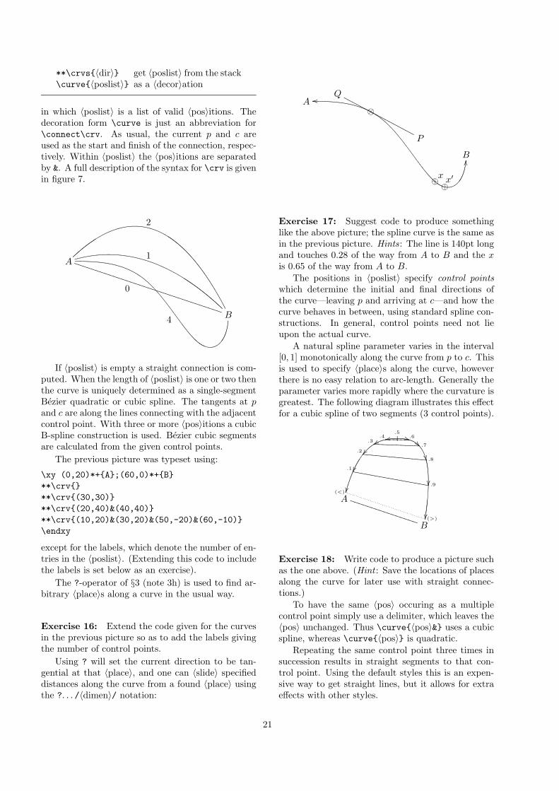
in which 〈poslist〉 is a list of valid 〈pos〉itions. Thedecoration form \curve is just an abbreviation for\connect\crv. As usual, the current p and c areused as the start and finish of the connection, respec-tively. Within 〈poslist〉 the 〈pos〉itions are separatedby &. A full description of the syntax for \crv is givenin figure 7.
A
BTTTTTTTTTTTTTTTTTTTTTTTTTTTTTTTTTT
0
1
2
4
If 〈poslist〉 is empty a straight connection is com-puted. When the length of 〈poslist〉 is one or two thenthe curve is uniquely determined as a single-segmentBezier quadratic or cubic spline. The tangents at pand c are along the lines connecting with the adjacentcontrol point. With three or more 〈pos〉itions a cubicB-spline construction is used. Bezier cubic segmentsare calculated from the given control points.
The previous picture was typeset using:
\xy (0,20)*+{A};(60,0)*+{B}**\crv{}**\crv{(30,30)}**\crv{(20,40)&(40,40)}**\crv{(10,20)&(30,20)&(50,-20)&(60,-10)}\endxy
except for the labels, which denote the number of en-tries in the 〈poslist〉. (Extending this code to includethe labels is set below as an exercise).
The ?-operator of §3 (note 3h) is used to find ar-bitrary 〈place〉s along a curve in the usual way.
Exercise 16: Extend the code given for the curvesin the previous picture so as to add the labels givingthe number of control points.
Using ? will set the current direction to be tan-gential at that 〈place〉, and one can 〈slide〉 specifieddistances along the curve from a found 〈place〉 usingthe ?. . . /〈dimen〉/ notation:
A
B
oo
NN
⊕x⊕x′
⊗
Q
P
NNNNNNNNNNNNNNNNN
Exercise 17: Suggest code to produce somethinglike the above picture; the spline curve is the same asin the previous picture. Hints: The line is 140pt longand touches 0.28 of the way from A to B and the xis 0.65 of the way from A to B.
The positions in 〈poslist〉 specify control pointswhich determine the initial and final directions ofthe curve—leaving p and arriving at c—and how thecurve behaves in between, using standard spline con-structions. In general, control points need not lieupon the actual curve.
A natural spline parameter varies in the interval[0, 1] monotonically along the curve from p to c. Thisis used to specify 〈place〉s along the curve, howeverthere is no easy relation to arc-length. Generally theparameter varies more rapidly where the curvature isgreatest. The following diagram illustrates this effectfor a cubic spline of two segments (3 control points).
A
BTTTTTTTTTTTTTTTT
��
��
��
����
yy ��rr **�
(<)
(>)
.1
.9YYYYYYYYYYYYYYYYY
.2
.8\\\\\\\\\\\\\\.3
.7^^^^^^^^^^.4 .6______
.5
Exercise 18: Write code to produce a picture suchas the one above. (Hint : Save the locations of placesalong the curve for later use with straight connec-tions.)
To have the same 〈pos〉 occuring as a multiplecontrol point simply use a delimiter, which leaves the〈pos〉 unchanged. Thus \curve{〈pos〉&} uses a cubicspline, whereas \curve{〈pos〉} is quadratic.
Repeating the same control point three times insuccession results in straight segments to that con-trol point. Using the default styles this is an expen-sive way to get straight lines, but it allows for extraeffects with other styles.
21
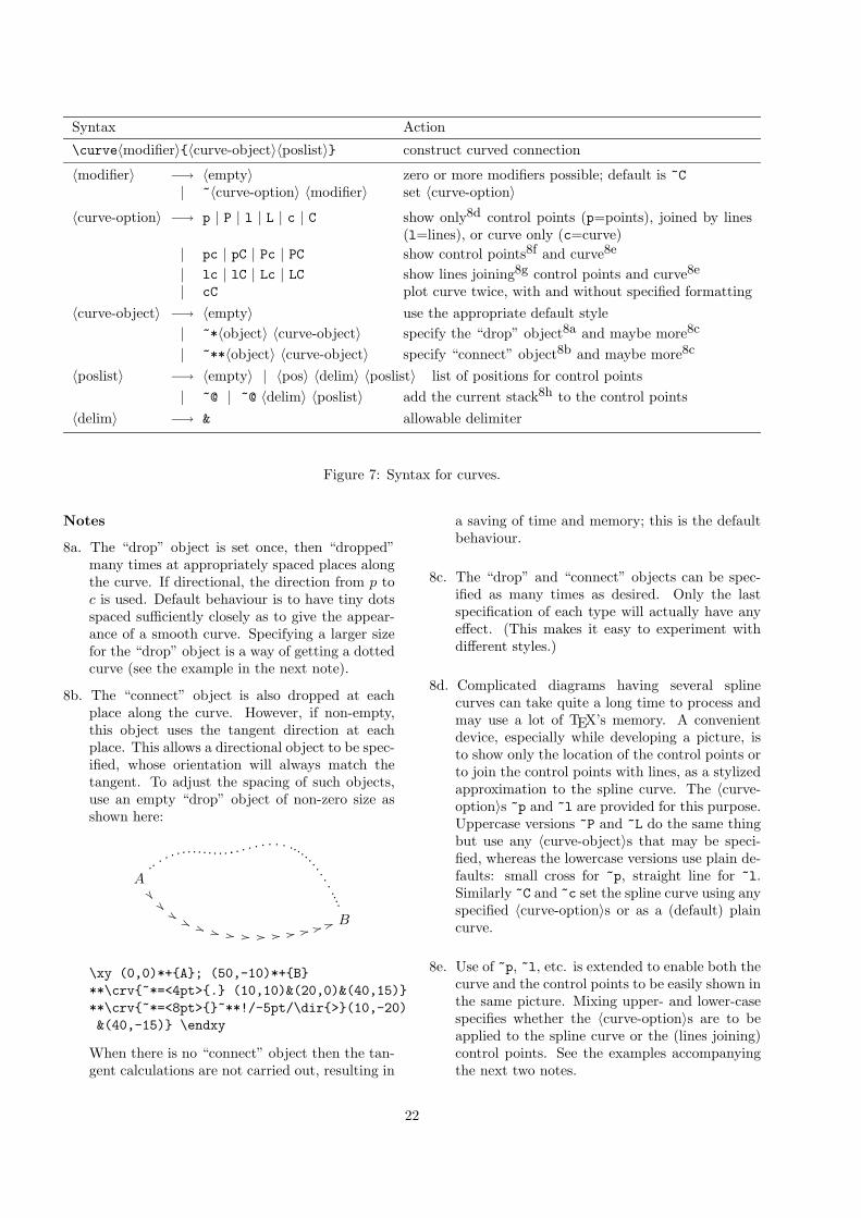
Syntax Action
\curve〈modifier〉{〈curve-object〉〈poslist〉} construct curved connection
〈modifier〉 −→ 〈empty〉 zero or more modifiers possible; default is ~C| ~〈curve-option〉 〈modifier〉 set 〈curve-option〉
〈curve-option〉 −→ p | P | l | L | c | C show only8d control points (p=points), joined by lines(l=lines), or curve only (c=curve)
| pc | pC | Pc | PC show control points8f and curve8e
| lc | lC | Lc | LC show lines joining8g control points and curve8e
| cC plot curve twice, with and without specified formatting〈curve-object〉 −→ 〈empty〉 use the appropriate default style
| ~*〈object〉 〈curve-object〉 specify the “drop” object8a and maybe more8c
| ~**〈object〉 〈curve-object〉 specify “connect” object8b and maybe more8c
〈poslist〉 −→ 〈empty〉 | 〈pos〉 〈delim〉 〈poslist〉 list of positions for control points| ~@ | ~@ 〈delim〉 〈poslist〉 add the current stack8h to the control points
〈delim〉 −→ & allowable delimiter
Figure 7: Syntax for curves.
Notes
8a. The “drop” object is set once, then “dropped”many times at appropriately spaced places alongthe curve. If directional, the direction from p toc is used. Default behaviour is to have tiny dotsspaced sufficiently closely as to give the appear-ance of a smooth curve. Specifying a larger sizefor the “drop” object is a way of getting a dottedcurve (see the example in the next note).
8b. The “connect” object is also dropped at eachplace along the curve. However, if non-empty,this object uses the tangent direction at eachplace. This allows a directional object to be spec-ified, whose orientation will always match thetangent. To adjust the spacing of such objects,use an empty “drop” object of non-zero size asshown here:
A
B
.. .. . . . . .... . . . .. .
. . . . . . . ...............����$$ '' )) ++ -- .. // 00 11 22
33 44
\xy (0,0)*+{A}; (50,-10)*+{B}**\crv{~*=<4pt>{.} (10,10)&(20,0)&(40,15)}**\crv{~*=<8pt>{}~**!/-5pt/\dir{>}(10,-20)&(40,-15)} \endxy
When there is no “connect” object then the tan-gent calculations are not carried out, resulting in
a saving of time and memory; this is the defaultbehaviour.
8c. The “drop” and “connect” objects can be spec-ified as many times as desired. Only the lastspecification of each type will actually have anyeffect. (This makes it easy to experiment withdifferent styles.)
8d. Complicated diagrams having several splinecurves can take quite a long time to process andmay use a lot of TEX’s memory. A convenientdevice, especially while developing a picture, isto show only the location of the control points orto join the control points with lines, as a stylizedapproximation to the spline curve. The 〈curve-option〉s ~p and ~l are provided for this purpose.Uppercase versions ~P and ~L do the same thingbut use any 〈curve-object〉s that may be speci-fied, whereas the lowercase versions use plain de-faults: small cross for ~p, straight line for ~l.Similarly ~C and ~c set the spline curve using anyspecified 〈curve-option〉s or as a (default) plaincurve.
8e. Use of ~p, ~l, etc. is extended to enable both thecurve and the control points to be easily shown inthe same picture. Mixing upper- and lower-casespecifies whether the 〈curve-option〉s are to beapplied to the spline curve or the (lines joining)control points. See the examples accompanyingthe next two notes.
22
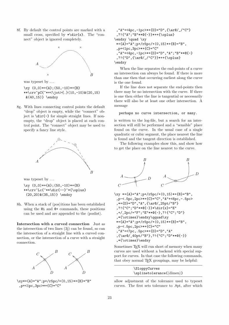
8f. By default the control points are marked with asmall cross, specified by *\dir{x}. The “con-nect” object is ignored completely.
A
B5u
5u 5u
...... . .............................................................
was typeset by . . .
\xy (0,0)*+{A};(50,-10)*+{B}**\crv~pC{~*=<\jot>{.}(10,-10)&(20,15)&(40,15)} \endxy
8g. With lines connecting control points the default“drop” object is empty, while the “connect” ob-ject is \dir{-} for simple straight lines. If non-empty, the “drop” object is placed at each con-trol point. The “connect” object may be used tospecify a fancy line style.
A
B
⊕��
��
��
�
⊕TTTT
22
22
22
22
was typeset by . . .
\xy (0,0)*+{A};(50,-10)*+{B}**\crv~Lc{~**\dir{--}~*{\oplus}(20,20)&(35,15)} \endxy
8h. When a stack of 〈pos〉itions has been establishedusing the @i and @+ commands, these positionscan be used and are appended to the 〈poslist〉.
Intersection with a curved connection Just asthe intersection of two lines (3j) can be found, so canthe intersection of a straight line with a curved con-nection, or the intersection of a curve with a straightconnection.
A
BC
D
cc vvvvvvvvvvvv
⊕
A
BC
D
vvvvvvvvvvvv
cc⊕
\xy*+{A}="A";p+/r5pc/+(0,15)*+{B}="B",p+<1pc,3pc>*+{C}="C"
,"A"+<4pc,-1pc>*+{D}="D",{\ar@/_/"C"},?!{"A";"B"**@{-}}*++{\oplus}
\endxy \quad \xy*+{A}="A";p+/r5pc/+(0,15)*+{B}="B",,p+<1pc,3pc>*+{C}="C","A"+<4pc,-1pc>*+{D}="D","A";"B"**@{-},?!{"D",{\ar@/_/"C"}}*++{\oplus}
\endxy
When the line separates the end-points of a curvean intersection can always be found. If there is morethan one then that occurring earliest along the curveis the one found.
If the line does not separate the end-points thenthere may be no intersection with the curve. If thereis one then either the line is tangential or necessarilythere will also be at least one other intersection. Amessage
perhaps no curve intersection, or many.
is written to the log-file, but a search for an inter-section will still be performed and a “sensible” placefound on the curve. In the usual case of a singlequadratic or cubic segment, the place nearest the lineis found and the tangent direction is established.
The following examples show this, and show howto get the place on the line nearest to the curve.
A
B
C
D
NN
ffffffffffffff
K�&&&&&⊗
A
B
C
D
RR
jjjjjjjjjjjjjjjjj⊗
\xy *+{A}="A";p+/r5pc/+(0,15)*+{B}="B",,p-<.5pc,2pc>*+{C}="C","A"+<6pc,-.5pc>,*+{D}="D","A",{\ar@/_25pt/"B"},?!{"C";"D"**@{-}}*\dir{x}="E",+/_2pc/="F";"E"**@{-},?!{"C";"D"},*{\otimes}\endxy\qquad\xy*+{A}="A";p+/r5pc/+(0,15)*+{B}="B",,p-<.5pc,2pc>*+{C}="C","A"+<7pc,.5pc>*+{D}="D","A",{\ar@/_40pt/"B"},?!{"C";"D"**@{-}},*{\otimes}\endxy
Sometimes TEX will run short of memory when manycurves are used without a backend with special sup-port for curves. In that case the following commands,that obey normal TEX groupings, may be helpful:
\SloppyCurves\splinetolerance{〈dimen〉}
allow adjustment of the tolerance used to typesetcurves. The first sets tolerance to .8pt, after which
23
\splinetolerance{0pt} resets to the original de-fault of fine curves.
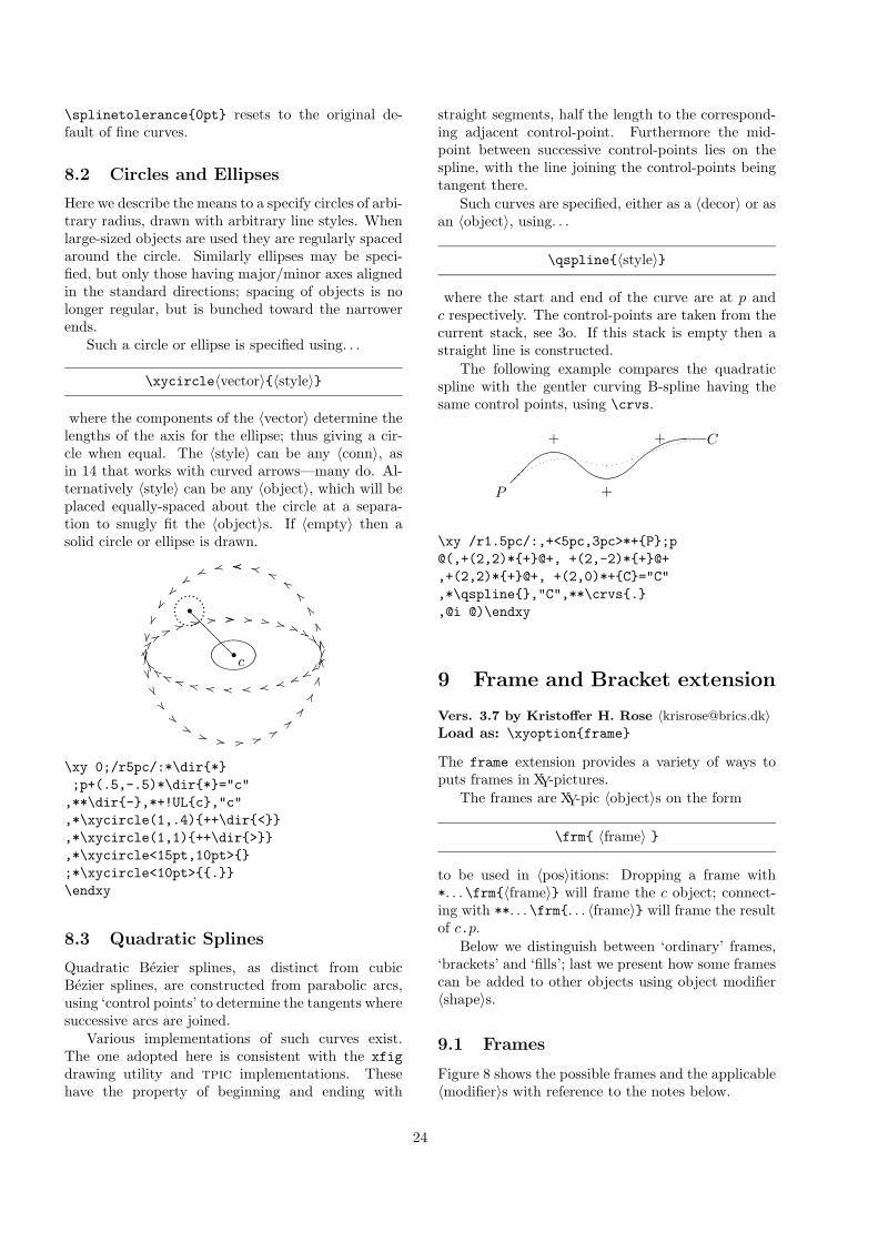
8.2 Circles and Ellipses
Here we describe the means to a specify circles of arbi-trary radius, drawn with arbitrary line styles. Whenlarge-sized objects are used they are regularly spacedaround the circle. Similarly ellipses may be speci-fied, but only those having major/minor axes alignedin the standard directions; spacing of objects is nolonger regular, but is bunched toward the narrowerends.
Such a circle or ellipse is specified using. . .
\xycircle〈vector〉{〈style〉}
where the components of the 〈vector〉 determine thelengths of the axis for the ellipse; thus giving a cir-cle when equal. The 〈style〉 can be any 〈conn〉, asin 14 that works with curved arrows—many do. Al-ternatively 〈style〉 can be any 〈object〉, which will beplaced equally-spaced about the circle at a separa-tion to snugly fit the 〈object〉s. If 〈empty〉 then asolid circle or ellipse is drawn.
•
•?????????
c
//0022336699@@IIQQ ZZ bb gg jj kk mm nn pp qq ssuu ww|| �� ����%%
((++,,..//
oorrvvzz���� ��������!!&& ** -- 11 44
88==CCGGKKNNRRUUYY^^dd
hhlloo
.......................
\xy 0;/r5pc/:*\dir{*};p+(.5,-.5)*\dir{*}="c"
,**\dir{-},*+!UL{c},"c",*\xycircle(1,.4){++\dir{<}},*\xycircle(1,1){++\dir{>}},*\xycircle<15pt,10pt>{};*\xycircle<10pt>{{.}}\endxy
8.3 Quadratic Splines
Quadratic Bezier splines, as distinct from cubicBezier splines, are constructed from parabolic arcs,using ‘control points’ to determine the tangents wheresuccessive arcs are joined.
Various implementations of such curves exist.The one adopted here is consistent with the xfigdrawing utility and tpic implementations. Thesehave the property of beginning and ending with
straight segments, half the length to the correspond-ing adjacent control-point. Furthermore the mid-point between successive control-points lies on thespline, with the line joining the control-points beingtangent there.
Such curves are specified, either as a 〈decor〉 or asan 〈object〉, using. . .
\qspline{〈style〉}
where the start and end of the curve are at p andc respectively. The control-points are taken from thecurrent stack, see 3o. If this stack is empty then astraight line is constructed.
The following example compares the quadraticspline with the gentler curving B-spline having thesame control points, using \crvs.
P
+
+
+ C
����
___
\xy /r1.5pc/:,+<5pc,3pc>*+{P};p@(,+(2,2)*{+}@+, +(2,-2)*{+}@+,+(2,2)*{+}@+, +(2,0)*+{C}="C",*\qspline{},"C",**\crvs{.},@i @)\endxy
9 Frame and Bracket extension
Vers. 3.7 by Kristoffer H. Rose 〈[email protected]〉Load as: \xyoption{frame}
The frame extension provides a variety of ways toputs frames in XY-pictures.
The frames are XY-pic 〈object〉s on the form
\frm{ 〈frame〉 }
to be used in 〈pos〉itions: Dropping a frame with*. . . \frm{〈frame〉} will frame the c object; connect-ing with **. . . \frm{. . . 〈frame〉} will frame the resultof c.p.
Below we distinguish between ‘ordinary’ frames,‘brackets’ and ‘fills’; last we present how some framescan be added to other objects using object modifier〈shape〉s.
9.1 Frames
Figure 8 shows the possible frames and the applicable〈modifier〉s with reference to the notes below.
24
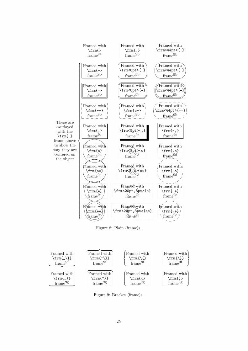
Framed with\frm{}frame9a
Framed with\frm{.}frame9b
Framed with\frm<44pt>{.}
frame9b
Framed with\frm{-}frame9b
Framed with\frm<8pt>{-}
frame9b
?> =<89 :;
Framed with\frm<44pt>{-}
frame9b
_^ ]\XY Z[
Framed with\frm{=}frame9b
Framed with\frm<8pt>{=}
frame9b
?> =<89 :;/. -,() *+
Framed with\frm<44pt>{=}
frame9b
_^ ]\XY Z[_^ ]\XY Z[
Framed with\frm{--}frame9b
_ _ _ _ _ _����
����
_ _ _ _ _ _
Framed with\frm{o-}frame9b
�� _ _ _ _ ���
�
�
��� _ _ _ _ ��Framed with
\frm<44pt>{--}
frame9b
_v�
_ _ _ _ _
�6T
�� ���6
T _ _ _ _ __ v�
Framed with\frm{,}frame9c
Framed with\frm<5pt>{,}
frame9c
Framed with\frm{-,}frame9c
Framed with\frm{o}frame9d
wvutpqrs Framed with\frm<8pt>{o}
frame9d
?>=<89:; Framed with\frm{.o}frame9d
Framed with\frm{oo}frame9d
wvutpqrswvutpqrs Framed with\frm<8pt>{oo}
frame9d
?>=<89:;'&%$ !"# Framed with\frm{-o}frame9d
_jx
� �
*8
JW
�*
8J W _ j x
�
Framed with\frm{e}frame9e
onmlhijk Framed with\frm<20pt,8pt>{e}
frame9e
WVUTPQRS Framed with\frm{.e}frame9e
Framed with\frm{ee}frame9e
onmlhijkgfed`abc Framed with\frm<20pt,8pt>{ee}
frame9e
WVUTPQRSONMLHIJK Framed with\frm{-e}frame9e
_n�
� �.
BT
�.
BT _ n �
�
These areoverlayedwith the\frm{.}
frame aboveto show theway they arecentered onthe object
Figure 8: Plain 〈frame〉s.
Framed with\frm{_\}}
frame9f︸ ︷︷ ︸Framed with\frm{^\}}
frame9f
︷ ︸︸ ︷Framed with\frm{\{}frame9f
Framed with\frm{\}}frame9f
Framed with\frm{_)}frame9g︸ ︸
Framed with\frm{^)}frame9g
︷ ︷Framed with\frm{(}frame9g
Framed with\frm{)}frame9g
Figure 9: Bracket 〈frame〉s.
25
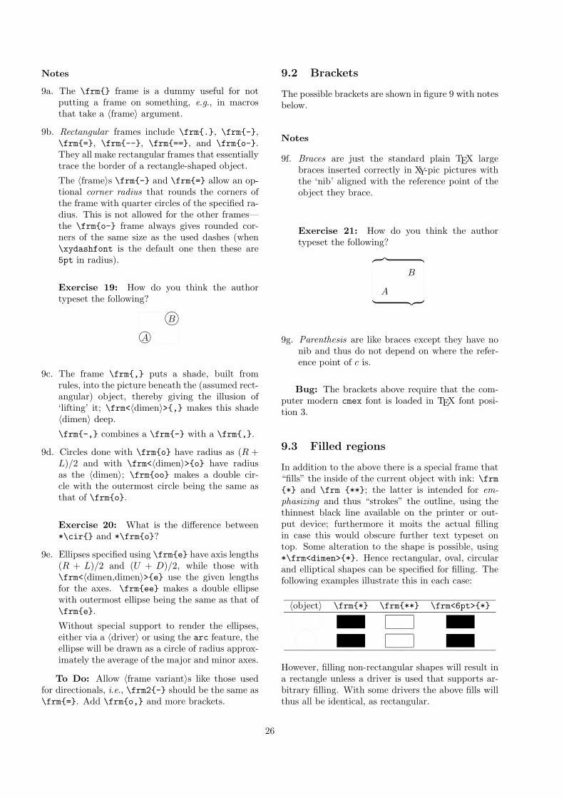
Notes
9a. The \frm{} frame is a dummy useful for notputting a frame on something, e.g., in macrosthat take a 〈frame〉 argument.
9b. Rectangular frames include \frm{.}, \frm{-},\frm{=}, \frm{--}, \frm{==}, and \frm{o-}.They all make rectangular frames that essentiallytrace the border of a rectangle-shaped object.
The 〈frame〉s \frm{-} and \frm{=} allow an op-tional corner radius that rounds the corners ofthe frame with quarter circles of the specified ra-dius. This is not allowed for the other frames—the \frm{o-} frame always gives rounded cor-ners of the same size as the used dashes (when\xydashfont is the default one then these are5pt in radius).
Exercise 19: How do you think the authortypeset the following?
A/.-,()*+B76540123
9c. The frame \frm{,} puts a shade, built fromrules, into the picture beneath the (assumed rect-angular) object, thereby giving the illusion of‘lifting’ it; \frm<〈dimen〉>{,} makes this shade〈dimen〉 deep.
\frm{-,} combines a \frm{-} with a \frm{,}.
9d. Circles done with \frm{o} have radius as (R +L)/2 and with \frm<〈dimen〉>{o} have radiusas the 〈dimen〉; \frm{oo} makes a double cir-cle with the outermost circle being the same asthat of \frm{o}.
Exercise 20: What is the difference between*\cir{} and *\frm{o}?
9e. Ellipses specified using \frm{e} have axis lengths(R + L)/2 and (U + D)/2, while those with\frm<〈dimen,dimen〉>{e} use the given lengthsfor the axes. \frm{ee} makes a double ellipsewith outermost ellipse being the same as that of\frm{e}.
Without special support to render the ellipses,either via a 〈driver〉 or using the arc feature, theellipse will be drawn as a circle of radius approx-imately the average of the major and minor axes.
To Do: Allow 〈frame variant〉s like those usedfor directionals, i.e., \frm2{-} should be the same as\frm{=}. Add \frm{o,} and more brackets.
9.2 Brackets
The possible brackets are shown in figure 9 with notesbelow.
Notes
9f. Braces are just the standard plain TEX largebraces inserted correctly in XY-pic pictures withthe ‘nib’ aligned with the reference point of theobject they brace.
Exercise 21: How do you think the authortypeset the following?
A
B
︷ ︸︸ ︷︸ ︷︷ ︸
9g. Parenthesis are like braces except they have nonib and thus do not depend on where the refer-ence point of c is.
Bug: The brackets above require that the com-puter modern cmex font is loaded in TEX font posi-tion 3.
9.3 Filled regions
In addition to the above there is a special frame that“fills” the inside of the current object with ink: \frm{*} and \frm {**}; the latter is intended for em-phasizing and thus “strokes” the outline, using thethinnest black line available on the printer or out-put device; furthermore it moits the actual fillingin case this would obscure further text typeset ontop. Some alteration to the shape is possible, using*\frm<dimen>{*}. Hence rectangular, oval, circularand elliptical shapes can be specified for filling. Thefollowing examples illustrate this in each case:
〈object〉 \frm{*} \frm{**} \frm<6pt>{*}
However, filling non-rectangular shapes will result ina rectangle unless a driver is used that supports ar-bitrary filling. With some drivers the above fills willthus all be identical, as rectangular.
26
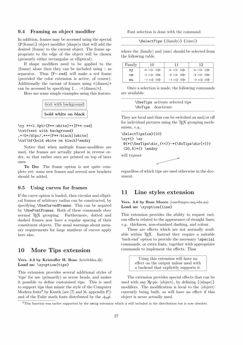
9.4 Framing as object modifier
In addition, frames may be accessed using the special[F〈frame〉] object modifier 〈shape〉s that will add thedesired 〈frame〉 to the current object. The frame ap-propriate to the edge of the object will be chosen(presently either rectangular or elliptical).
If shape modifiers need to be applied to the〈frame〉 alone then they can be included using : asseparator. Thus [F-:red] will make a red frame(provided the color extension is active, of course).Additionally the variant of frames using <〈dimen〉>can be accessed by specifying [. . . :<〈dimen〉>].
Here are some simple examples using this feature.
text with background
bold white on black
\xy *+<1.5pt>[F**:white]++[F**:red]\txt{text with background},+!D+/d1pc/,*++[F**:black][white]\txt\bf{bold white on black}\endxy
Notice that when multiple frame-modifiers areused, the frames are actually placed in reverse or-der, so that earlier ones are printed on top of laterones.
To Do: The frame option is not quite com-plete yet: some new frames and several new bracketsshould be added.
9.5 Using curves for frames
If the curve option is loaded, then circular and ellipti-cal frames of arbitrary radius can be constructed, byspecifying \UseCurvedFrames. This can be negatedby \UseFontFrames. Both of these commands obeynormal TEX grouping. Furthermore, dotted anddashed frames now have a regular spacing of theirconstituent objects. The usual warnings about mem-ory requirements for large numbers of curves applyhere also.
10 More Tips extension
Vers. 3.3 by Kristoffer H. Rose 〈[email protected]〉Load as: \xyoption{tips}
This extension provides several additional styles of‘tips’ for use (primarily) as arrow heads, and makesit possible to define customised tips. This is usedto support tips that mimic the style of the ComputerModern fonts8 by Knuth (see [7] and [6, appendix F])and of the Euler math fonts distributed by the AMS.
Font selection is done with the command
\SelectTips {〈family〉} {〈size〉}
where the 〈family〉 and 〈size〉 should be selected fromthe following table.
Family 10 11 12xy //− +3 _*4 //− +3 _*4 //− +3 _ *4
cm //− +3 _*4 //− +3 _*4 //− +3 _ *4
eu //− %9 _%9 //− %9 _%9 //− %9 _ %9
Once a selection is made, the following commandsare available:
\UseTips activate selected tips\NoTips deactivate
They are local and thus can be switched on and/or offfor individual pictures using the TEX grouping mech-anism, e.g.,
\SelectTips{cm}{10}\xy*{} \ar@{*{\UseTips\dir_{<<}}-*{\NoTips\dir{>}}}(20,5)*{} \endxy
will typeset
ss
33gggggggggggg
regardless of which tips are used otherwise in the doc-ument.
11 Line styles extension
Vers. 3.6 by Ross Moore 〈[email protected]〉Load as: \xyoption{line}
This extension provides the ability to request vari-ous effects related to the appearance of straight lines;e.g.. thickness, non-standard dashing, and colour.
These are effects which are not normally avail-able within TEX. Instead they require a suitable‘back-end’ option to provide the necessary \specialcommands, or extra fonts, together with appropriatecommands to implement the effects. Thus
Using this extension will have noeffect on the output unless used witha backend that explicitly supports it.
The extension provides special effects that can beused with any XY-pic 〈object〉, by defining [〈shape〉]modifiers. The modification is local to the 〈object〉currently being built, so will have no effect if thisobject is never actually used.
8This function was earlier supported by the cmtip extension which is still included in the distribution but is now obsolete.
27
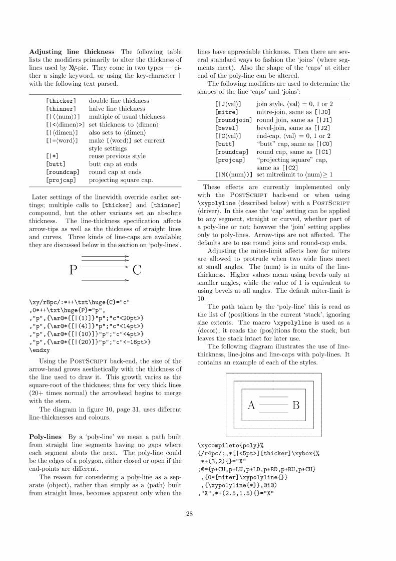
Adjusting line thickness The following tablelists the modifiers primarily to alter the thickness oflines used by XY-pic. They come in two types — ei-ther a single keyword, or using the key-character |with the following text parsed.
[thicker] double line thickness[thinner] halve line thickness[|(〈num〉)] multiple of usual thickness[|<〈dimen〉>] set thickness to 〈dimen〉[|〈dimen〉] also sets to 〈dimen〉[|=〈word〉] make [〈word〉] set current
style settings[|*] reuse previous style[butt] butt cap at ends[roundcap] round cap at ends[projcap] projecting square cap.
Later settings of the linewidth override earlier set-tings; multiple calls to [thicker] and [thinner]compound, but the other variants set an absolutethickness. The line-thickness specification affectsarrow-tips as well as the thickness of straight linesand curves. Three kinds of line-caps are available;they are discussed below in the section on ‘poly-lines’.
CP
//////
//
\xy/r8pc/:*++\txt\huge{C}="c",0*++\txt\huge{P}="p",,"p",{\ar@*{[|(1)]}"p";"c"<20pt>},"p",{\ar@*{[|(4)]}"p";"c"<14pt>},"p",{\ar@*{[|(10)]}"p";"c"<4pt>},"p",{\ar@*{[|(20)]}"p";"c"<-16pt>}\endxy
Using the PostScript back-end, the size of thearrow-head grows aesthetically with the thickness ofthe line used to draw it. This growth varies as thesquare-root of the thickness; thus for very thick lines(20+ times normal) the arrowhead begins to mergewith the stem.
The diagram in figure 10, page 31, uses differentline-thicknesses and colours.
Poly-lines By a ‘poly-line’ we mean a path builtfrom straight line segments having no gaps whereeach segment abuts the next. The poly-line couldbe the edges of a polygon, either closed or open if theend-points are different.
The reason for considering a poly-line as a sep-arate 〈object〉, rather than simply as a 〈path〉 builtfrom straight lines, becomes apparent only when the
lines have appreciable thickness. Then there are sev-eral standard ways to fashion the ‘joins’ (where seg-ments meet). Also the shape of the ‘caps’ at eitherend of the poly-line can be altered.
The following modifiers are used to determine theshapes of the line ‘caps’ and ‘joins’:
[|J〈val〉] join style, 〈val〉 = 0, 1 or 2[mitre] mitre-join, same as [|J0][roundjoin] round join, same as [|J1][bevel] bevel-join, same as [|J2][|C〈val〉] end-cap, 〈val〉 = 0, 1 or 2[butt] “butt” cap, same as [|C0][roundcap] round cap, same as [|C1][projcap] “projecting square” cap,
same as [|C2][|M(〈num〉)] set mitrelimit to 〈num〉≥ 1
These effects are currently implemented onlywith the PostScript back-end or when using\xypolyline (described below) with a PostScript
〈driver〉. In this case the ‘cap’ setting can be appliedto any segment, straight or curved, whether part ofa poly-line or not; however the ‘join’ setting appliesonly to poly-lines. Arrow-tips are not affected. Thedefaults are to use round joins and round-cap ends.
Adjusting the miter-limit affects how far mitersare allowed to protrude when two wide lines meetat small angles. The 〈num〉 is in units of the line-thickness. Higher values mean using bevels only atsmaller angles, while the value of 1 is equivalent tousing bevels at all angles. The default miter-limit is10.
The path taken by the ‘poly-line’ this is read asthe list of 〈pos〉itions in the current ‘stack’, ignoringsize extents. The macro \xypolyline is used as a〈decor〉; it reads the 〈pos〉itions from the stack, butleaves the stack intact for later use.
The following diagram illustrates the use of line-thickness, line-joins and line-caps with poly-lines. Itcontains an example of each of the styles.
A B
\xycompileto{poly}%{/r4pc/:,*[|<5pt>][thicker]\xybox{%*+(3,2){}="X"
;@={p+CU,p+LU,p+LD,p+RD,p+RU,p+CU},{0*[miter]\xypolyline{}},{\xypolyline{*}},@i@)
,"X",*+(2.5,1.5){}="X"
28
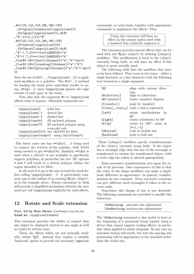
,@={!CU,!LU,!LD,!RD,!RU,!CU},{0*[gray][roundjoin]\xypolyline{}},{0*[gray]\xypolyline{*}},@i@)
,"X",*+(2,1){}="X",@={!CU,!LU,!LD,!RD,!RU,!CU},{0*[white]\xypolyline{*}},{0*[bevel]\xypolyline{}},@i@)
,"X"-(.7,0)*++\txt\LARGE{A}="a","X"+(.7,0)*++\txt\LARGE{B}="b",{\ar@{-}@*{[butt][thinner]}"a";"b"<1pc>},{\ar@{-}@*{[roundcap][thinner]}"a";"b"},{\ar@{-}@*{[projcap][thinner]}"a";"b"<-1pc>}}}
Note the use of {0*[...]\xypolyline{..}} to applystyle-modifiers to a polyline. The @={!..} methodfor loading the stack gives equivalent results to us-ing ;@={p+..}, since \xypolyline ignores the edgeextents of each 〈pos〉 in the stack.
Note also that the argument #1 to \xypolylineaffects what is typeset. Allowable arguments are:
\xypolyline{} solid line\xypolyline{.} dotted line\xypolyline{-} dashed line\xypolyline{*} fill enclosed polygon\xypolyline{?} fill enclosed polygon using
even-odd rule\xypolyline{{*}} use \dir{*} for lines\xypolyline{<toks>} using \dir{<toks>}
The latter cases one has **\dir{...} being usedto connect the vertices of the polyline, with {{*}}being needed to get **\dir{*}. Similarly **\dir isused when a 〈driver〉 is not available to specificallysupport polylines; in particular the two ‘fill’ options* and ? will result in a dotted polygon outline theregion intended to be filled.
In all cases it is up to the user to load the stack be-fore calling \xypolyline{. . . }. A particularly com-mon case is the outline of an existing XY-pic 〈object〉,as in the example above. Future extensions to \frmwill provide a simplified mechanism whereby the userneed not call \xypolyline explicitly for such effects.
12 Rotate and Scale extension
Vers. 3.3 by Ross Moore 〈[email protected]〉Load as: \xyoption{rotate}
This extension provides the ability to request thatany object be displayed rotated at any angle as wellas scaled in various ways.
These are effects which are not normally avail-able within TEX. Instead they require a suitable‘back-end’ option to provide the necessary \special
commands, or extra fonts, together with appropriatecommands to implement the effects. Thus
Using this extension will have noeffect on the output unless used witha backend that explicitly supports it.
The extension provides special effects that can beused with any XY-pic 〈object〉 by defining [〈shape〉]modifiers. The modification is local to the 〈object〉currently being built, so will have no effect if thisobject is never actually used.
The following table lists the modifiers that haveso far been defined. They come in two types – either asingle keyword, or a key-character with the followingtext treated as a single argument.
[@] align with current direc-tion
[@〈direction〉] align to 〈direction〉[@!〈number〉] rotate 〈number〉 degrees[*〈number〉] scale by 〈number〉[*〈num〉x,〈num〉y] scale x and y separately[left] rotate anticlockwise by
90◦[right] rotate (clockwise) by 90◦
[flip] rotate by 180◦; same as[*-1,-1]
[dblsize] scale to double size[halfsize] scale to half size
These [〈shape〉] modifiers specify transformationsof the 〈object〉 currently being built. If the objecthas a rectangle edge then the size of the rectangle istransformed to enclose the transformed object; witha circle edge the radius is altered appropriately.
Each successive transformation acts upon the re-sult of all previous. One consequence of this is thatthe order of the shape modifiers can make a signif-icant difference in appearance—in general, transfor-mations do not commute. Even successive rotationscan give different sized rectangles if taken in the re-verse order.
Sometimes this change of size is not desirable.The following commands are provided to modify thisbehaviour.
\NoResizing prevents size adjustment\UseResizing restores size adjustments
The \NoResizing command is also useful to have atthe beginning of a document being typeset using adriver that cannot support scaling effects, in partic-ular when applied to whole diagrams. In any case anunscaled version will result, but now the spacing andpositioning will be appropriate to the unscaled ratherthan the scaled size.
29
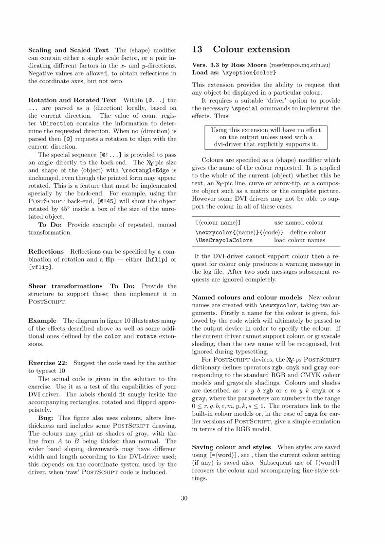
Scaling and Scaled Text The 〈shape〉 modifiercan contain either a single scale factor, or a pair in-dicating different factors in the x- and y-directions.Negative values are allowed, to obtain reflections inthe coordinate axes, but not zero.
Rotation and Rotated Text Within [@...] the... are parsed as a 〈direction〉 locally, based onthe current direction. The value of count regis-ter \Direction contains the information to deter-mine the requested direction. When no 〈direction〉 isparsed then [@] requests a rotation to align with thecurrent direction.
The special sequence [@!...] is provided to passan angle directly to the back-end. The XY-pic sizeand shape of the 〈object〉 with \rectangleEdge isunchanged, even though the printed form may appearrotated. This is a feature that must be implementedspecially by the back-end. For example, using thePostScript back-end, [@!45] will show the objectrotated by 45◦ inside a box of the size of the unro-tated object.
To Do: Provide example of repeated, namedtransformation.
Reflections Reflections can be specified by a com-bination of rotation and a flip — either [hflip] or[vflip].
Shear transformations To Do: Provide thestructure to support these; then implement it inPostScript.
Example The diagram in figure 10 illustrates manyof the effects described above as well as some addi-tional ones defined by the color and rotate exten-sions.
Exercise 22: Suggest the code used by the authorto typeset 10.
The actual code is given in the solution to theexercise. Use it as a test of the capabilities of yourDVI-driver. The labels should fit snugly inside theaccompanying rectangles, rotated and flipped appro-priately.
Bug: This figure also uses colours, alters line-thickness and includes some PostScript drawing.The colours may print as shades of gray, with theline from A to B being thicker than normal. Thewider band sloping downwards may have differentwidth and length according to the DVI-driver used;this depends on the coordinate system used by thedriver, when ‘raw’ PostScript code is included.
13 Colour extension
Vers. 3.3 by Ross Moore 〈[email protected]〉Load as: \xyoption{color}
This extension provides the ability to request thatany object be displayed in a particular colour.
It requires a suitable ‘driver’ option to providethe necessary \special commands to implement theeffects. Thus
Using this extension will have no effecton the output unless used with a
dvi-driver that explicitly supports it.
Colours are specified as a 〈shape〉 modifier whichgives the name of the colour requested. It is appliedto the whole of the current 〈object〉 whether this betext, an XY-pic line, curve or arrow-tip, or a compos-ite object such as a matrix or the complete picture.However some DVI drivers may not be able to sup-port the colour in all of these cases.
[〈colour name〉] use named colour
\newxycolor{〈name〉}{〈code〉} define colour\UseCrayolaColors load colour names
If the DVI-driver cannot support colour then a re-quest for colour only produces a warning message inthe log file. After two such messages subsequent re-quests are ignored completely.
Named colours and colour models New colournames are created with \newxycolor, taking two ar-guments. Firstly a name for the colour is given, fol-lowed by the code which will ultimately be passed tothe output device in order to specify the colour. Ifthe current driver cannot support colour, or grayscaleshading, then the new name will be recognised, butignored during typesetting.
For PostScript devices, the XY-ps PostScript
dictionary defines operators rgb, cmyk and gray cor-responding to the standard RGB and CMYK colourmodels and grayscale shadings. Colours and shadesare described as: r g b rgb or c m y k cmyk or sgray, where the parameters are numbers in the range0 ≤ r, g, b, c,m, y, k, s ≤ 1. The operators link to thebuilt-in colour models or, in the case of cmyk for ear-lier versions of PostScript, give a simple emulationin terms of the RGB model.
Saving colour and styles When styles are savedusing [=〈word〉], see , then the current colour setting(if any) is saved also. Subsequent use of [〈word〉]recovers the colour and accompanying line-style set-tings.
30
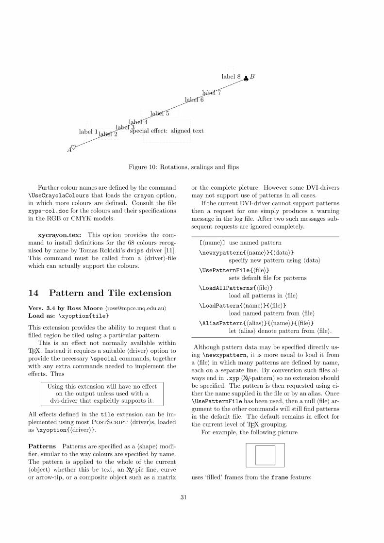
A
B
♥
♣llllllllllllllllllllllllllllllllllllllllllllllllllllllllll
label 1 .label 2×label 3
label 4label 5×
label 6label 7
label 8
special effect: aligned text
Figure 10: Rotations, scalings and flips
Further colour names are defined by the command\UseCrayolaColours that loads the crayon option,in which more colours are defined. Consult the filexyps-col.doc for the colours and their specificationsin the RGB or CMYK models.
xycrayon.tex: This option provides the com-mand to install definitions for the 68 colours recog-nised by name by Tomas Rokicki’s dvips driver [11].This command must be called from a 〈driver〉-filewhich can actually support the colours.
14 Pattern and Tile extension
Vers. 3.4 by Ross Moore 〈[email protected]〉Load as: \xyoption{tile}
This extension provides the ability to request that afilled region be tiled using a particular pattern.
This is an effect not normally available withinTEX. Instead it requires a suitable 〈driver〉 option toprovide the necessary \special commands, togetherwith any extra commands needed to implement theeffects. Thus
Using this extension will have no effecton the output unless used with a
dvi-driver that explicitly supports it.
All effects defined in the tile extension can be im-plemented using most PostScript 〈driver〉s, loadedas \xyoption{〈driver〉}.
Patterns Patterns are specified as a 〈shape〉 modi-fier, similar to the way colours are specified by name.The pattern is applied to the whole of the current〈object〉 whether this be text, an XY-pic line, curveor arrow-tip, or a composite object such as a matrix
or the complete picture. However some DVI-driversmay not support use of patterns in all cases.
If the current DVI-driver cannot support patternsthen a request for one simply produces a warningmessage in the log file. After two such messages sub-sequent requests are ignored completely.
[〈name〉] use named pattern
\newxypattern{〈name〉}{〈data〉}specify new pattern using 〈data〉
\UsePatternFile{〈file〉}sets default file for patterns
\LoadAllPatterns{〈file〉}load all patterns in 〈file〉
\LoadPattern{〈name〉}{〈file〉}load named pattern from 〈file〉
\AliasPattern{〈alias〉}{〈name〉}{〈file〉}let 〈alias〉 denote pattern from 〈file〉.
Although pattern data may be specified directly us-ing \newxypattern, it is more usual to load it froma 〈file〉 in which many patterns are defined by name,each on a separate line. By convention such files al-ways end in .xyp (XY-pattern) so no extension shouldbe specified. The pattern is then requested using ei-ther the name supplied in the file or by an alias. Once\UsePatternFile has been used, then a null 〈file〉 ar-gument to the other commands will still find patternsin the default file. The default remains in effect forthe current level of TEX grouping.
For example, the following picture
uses ‘filled’ frames from the frame feature:
31
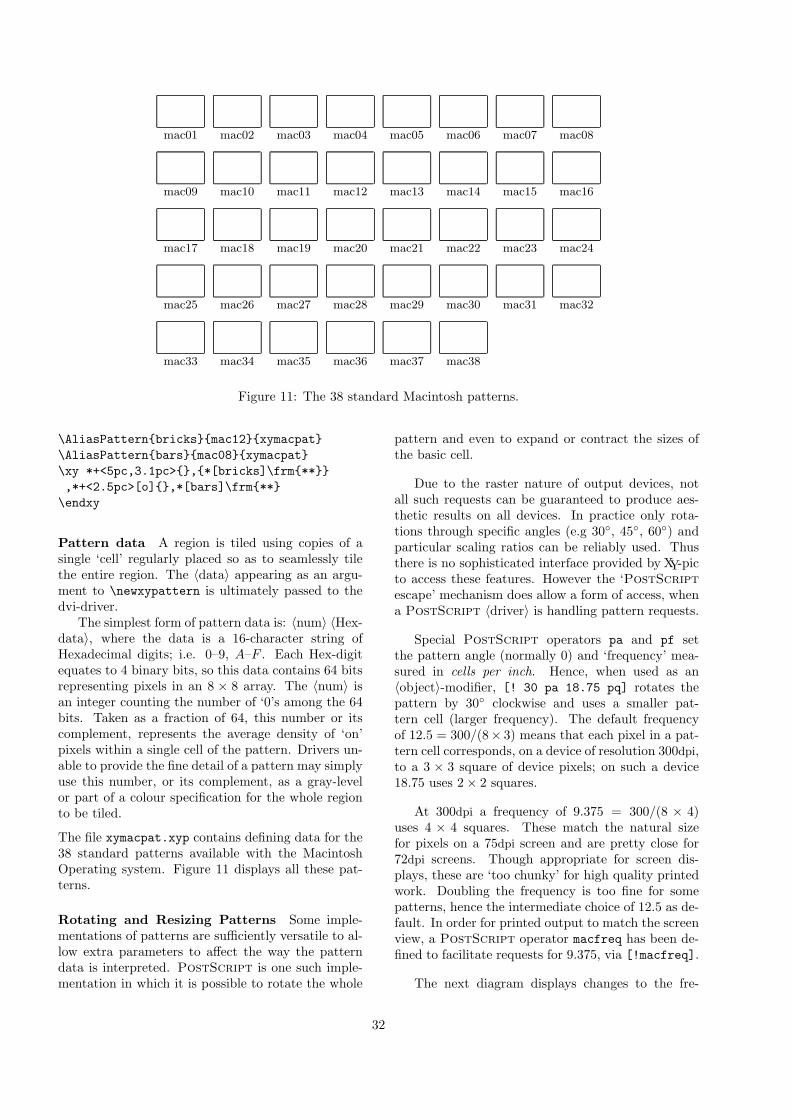
mac01 mac02 mac03 mac04 mac05 mac06 mac07 mac08
mac09 mac10 mac11 mac12 mac13 mac14 mac15 mac16
mac17 mac18 mac19 mac20 mac21 mac22 mac23 mac24
mac25 mac26 mac27 mac28 mac29 mac30 mac31 mac32
mac33 mac34 mac35 mac36 mac37 mac38
Figure 11: The 38 standard Macintosh patterns.
\AliasPattern{bricks}{mac12}{xymacpat}\AliasPattern{bars}{mac08}{xymacpat}\xy *+<5pc,3.1pc>{},{*[bricks]\frm{**}},*+<2.5pc>[o]{},*[bars]\frm{**}
\endxy
Pattern data A region is tiled using copies of asingle ‘cell’ regularly placed so as to seamlessly tilethe entire region. The 〈data〉 appearing as an argu-ment to \newxypattern is ultimately passed to thedvi-driver.
The simplest form of pattern data is: 〈num〉 〈Hex-data〉, where the data is a 16-character string ofHexadecimal digits; i.e. 0–9, A–F . Each Hex-digitequates to 4 binary bits, so this data contains 64 bitsrepresenting pixels in an 8 × 8 array. The 〈num〉 isan integer counting the number of ‘0’s among the 64bits. Taken as a fraction of 64, this number or itscomplement, represents the average density of ‘on’pixels within a single cell of the pattern. Drivers un-able to provide the fine detail of a pattern may simplyuse this number, or its complement, as a gray-levelor part of a colour specification for the whole regionto be tiled.
The file xymacpat.xyp contains defining data for the38 standard patterns available with the MacintoshOperating system. Figure 11 displays all these pat-terns.
Rotating and Resizing Patterns Some imple-mentations of patterns are sufficiently versatile to al-low extra parameters to affect the way the patterndata is interpreted. PostScript is one such imple-mentation in which it is possible to rotate the whole
pattern and even to expand or contract the sizes ofthe basic cell.
Due to the raster nature of output devices, notall such requests can be guaranteed to produce aes-thetic results on all devices. In practice only rota-tions through specific angles (e.g 30◦, 45◦, 60◦) andparticular scaling ratios can be reliably used. Thusthere is no sophisticated interface provided by XY-picto access these features. However the ‘PostScript
escape’ mechanism does allow a form of access, whena PostScript 〈driver〉 is handling pattern requests.
Special PostScript operators pa and pf setthe pattern angle (normally 0) and ‘frequency’ mea-sured in cells per inch. Hence, when used as an〈object〉-modifier, [! 30 pa 18.75 pq] rotates thepattern by 30◦ clockwise and uses a smaller pat-tern cell (larger frequency). The default frequencyof 12.5 = 300/(8× 3) means that each pixel in a pat-tern cell corresponds, on a device of resolution 300dpi,to a 3 × 3 square of device pixels; on such a device18.75 uses 2× 2 squares.
At 300dpi a frequency of 9.375 = 300/(8 × 4)uses 4 × 4 squares. These match the natural sizefor pixels on a 75dpi screen and are pretty close for72dpi screens. Though appropriate for screen dis-plays, these are ‘too chunky’ for high quality printedwork. Doubling the frequency is too fine for somepatterns, hence the intermediate choice of 12.5 as de-fault. In order for printed output to match the screenview, a PostScript operator macfreq has been de-fined to facilitate requests for 9.375, via [!macfreq].
The next diagram displays changes to the fre-
32
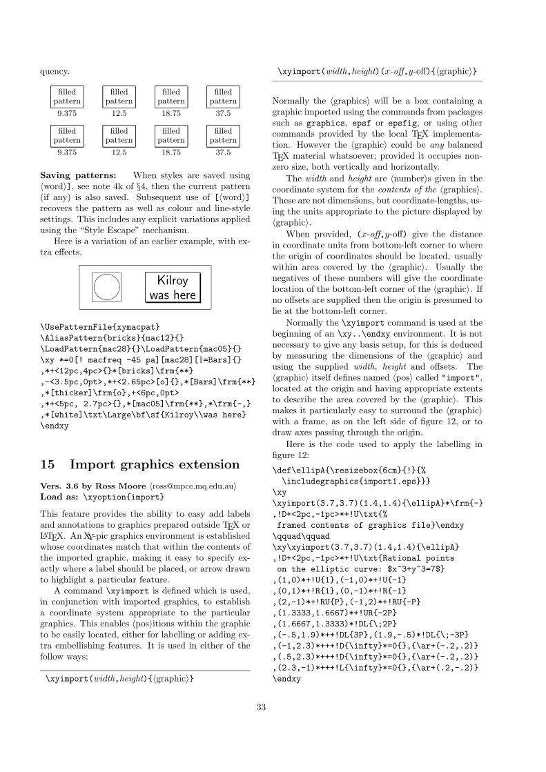
quency.
filledpattern
9.375
filledpattern
12.5
filledpattern
18.75
filledpattern
37.5
filledpattern
9.375
filledpattern
12.5
filledpattern
18.75
filledpattern
37.5
Saving patterns: When styles are saved using〈word〉], see note 4k of §4, then the current pattern(if any) is also saved. Subsequent use of [〈word〉]recovers the pattern as well as colour and line-stylesettings. This includes any explicit variations appliedusing the “Style Escape” mechanism.
Here is a variation of an earlier example, with ex-tra effects.
WVUTPQRS Kilroywas here
\UsePatternFile{xymacpat}\AliasPattern{bricks}{mac12}{}\LoadPattern{mac28}{}\LoadPattern{mac05}{}\xy *=0[! macfreq -45 pa][mac28][|=Bars]{},*+<12pc,4pc>{}*[bricks]\frm{**},-<3.5pc,0pt>,*+<2.65pc>[o]{},*[Bars]\frm{**},*[thicker]\frm{o},+<6pc,0pt>,*+<5pc, 2.7pc>{},*[mac05]\frm{**},*\frm{-,},*[white]\txt\Large\bf\sf{Kilroy\\was here}\endxy
15 Import graphics extension
Vers. 3.6 by Ross Moore 〈[email protected]〉Load as: \xyoption{import}
This feature provides the ability to easy add labelsand annotations to graphics prepared outside TEX orLATEX. An XY-pic graphics environment is establishedwhose coordinates match that within the contents ofthe imported graphic, making it easy to specify ex-actly where a label should be placed, or arrow drawnto highlight a particular feature.
A command \xyimport is defined which is used,in conjunction with imported graphics, to establisha coordinate system appropriate to the particulargraphics. This enables 〈pos〉itions within the graphicto be easily located, either for labelling or adding ex-tra embellishing features. It is used in either of thefollow ways:
\xyimport(width,height){〈graphic〉}
\xyimport(width,height)(x-off,y-off){〈graphic〉}
Normally the 〈graphics〉 will be a box containing agraphic imported using the commands from packagessuch as graphics, epsf or epsfig, or using othercommands provided by the local TEX implementa-tion. However the 〈graphic〉 could be any balancedTEX material whatsoever; provided it occupies non-zero size, both vertically and horizontally.
The width and height are 〈number〉s given in thecoordinate system for the contents of the 〈graphics〉.These are not dimensions, but coordinate-lengths, us-ing the units appropriate to the picture displayed by〈graphic〉.
When provided, (x-off,y-off) give the distancein coordinate units from bottom-left corner to wherethe origin of coordinates should be located, usuallywithin area covered by the 〈graphic〉. Usually thenegatives of these numbers will give the coordinatelocation of the bottom-left corner of the 〈graphic〉. Ifno offsets are supplied then the origin is presumed tolie at the bottom-left corner.
Normally the \xyimport command is used at thebeginning of an \xy..\endxy environment. It is notnecessary to give any basis setup, for this is deducedby measuring the dimensions of the 〈graphic〉 andusing the supplied width, height and offsets. The〈graphic〉 itself defines named 〈pos〉 called "import",located at the origin and having appropriate extentsto describe the area covered by the 〈graphic〉. Thismakes it particularly easy to surround the 〈graphic〉with a frame, as on the left side of figure 12, or todraw axes passing through the origin.
Here is the code used to apply the labelling infigure 12:
\def\ellipA{\resizebox{6cm}{!}{%\includegraphics{import1.eps}}}
\xy\xyimport(3.7,3.7)(1.4,1.4){\ellipA}*\frm{-},!D+<2pc,-1pc>*+!U\txt{%framed contents of graphics file}\endxy
\qquad\qquad\xy\xyimport(3.7,3.7)(1.4,1.4){\ellipA},!D+<2pc,-1pc>*+!U\txt{Rational pointson the elliptic curve: $x^3+y^3=7$}
,(1,0)*+!U{1},(-1,0)*+!U{-1},(0,1)*+!R{1},(0,-1)*+!R{-1},(2,-1)*+!RU{P},(-1,2)*+!RU{-P},(1.3333,1.6667)*+!UR{-2P},(1.6667,1.3333)*!DL{\;2P},(-.5,1.9)*++!DL{3P},(1.9,-.5)*!DL{\;-3P},(-1,2.3)*+++!D{\infty}*=0{},{\ar+(-.2,.2)},(.5,2.3)*+++!D{\infty}*=0{},{\ar+(-.2,.2)},(2.3,-1)*+++!L{\infty}*=0{},{\ar+(.2,-.2)}\endxy
33
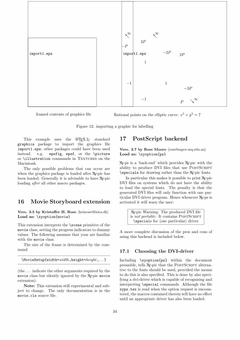
import1.eps
framed contents of graphics file
import1.eps
Rational points on the elliptic curve: x3 + y3 = 7
1−1
1
−1P
−P−2P 2P
3P
−3P
∞__???∞__???
∞��???
Figure 12: importing a graphic for labelling
This example uses the LATEX 2ε standardgraphics package to import the graphics fileimport1.eps; other packages could have been usedinstead. e.g. epsfig, epsf, or the \pictureor \illustration commands in Textures on theMacintosh.
The only possible problems that can occur arewhen the graphics package is loaded after XY-pic hasbeen loaded. Generally it is advisable to have XY-picloading after all other macro packages.
16 Movie Storyboard extension
Vers. 3.5 by Kristoffer H. Rose 〈[email protected]〉Load as: \xyoption{movie}
This extension interprets the \scene primitive of themovie class, setting the progress indicators to dummyvalues. The following assumes that your are familiarwith the movie class.
The size of the frame is determined by the com-mand
\MovieSetup{width=width,height=height,. . . }
(the . . . indicate the other arguments required by themovie class but silently ignored by the XY-pic movieextension).
Note: This extension still experimental and sub-ject to change. The only documentation is in themovie.cls source file.
17 PostScript backend
Vers. 3.7 by Ross Moore 〈[email protected]〉Load as: \xyoption{ps}
XY-ps is a ‘back-end’ which provides XY-pic with theability to produce DVI files that use PostScript
\specials for drawing rather than the XY-pic fonts.In particular this makes it possible to print XY-pic
DVI files on systems which do not have the abilityto load the special fonts. The penalty is that thegenerated DVI files will only function with one par-ticular DVI driver program. Hence whenever XY-ps isactivated it will warn the user:
XY-pic Warning: The produced DVI fileis not portable: It contains PostScript
\specials for 〈one particular〉 driver
A more complete discussion of the pros and cons ofusing this backend is included below.
17.1 Choosing the DVI-driver
Including \xyoption{ps} within the documentpreamble, tells XY-pic that the PostScript alterna-tive to the fonts should be used, provided the meansto do this is also specified. This is done by also speci-fying a dvi-driver which is capable of recognising andinterpreting \special commands. Although the filexyps.tex is read when the option request is encoun-tered, the macros contained therein will have no effectuntil an appropriate driver has also been loaded.
34
With LATEX 2ε both the backend and driver maybe specified, along with other options, via a single\usepackage command, see [4, page 317]; e.g.
\usepackage[ps,textures,color,arrow]{xy}
The rebindings necessary to support PostScript arenot effected until the \begin{document} command isencountered. This means that an alternative drivermay be selected, by another \xyoption{〈driver〉},at any time until the \begin{document}. Only themacros relevant to last named 〈driver〉 will actuallybe installed.
The following table describes available support forPostScript drivers. Please consult the individualdriver sections in part IV for the exact current list.For each 〈driver〉 there is a corresponding file namedxy〈driver〉.tex which defines the necessary macros,as well as a documentation file named xy〈driver〉.doc.The spelling is all lower-case, designed to be both de-scriptive and unique for the 1st 8 characters of thefile names.
〈driver〉 Descriptiondvips Tomas Rokicki’s dvips
dvips Karl Berry’s dvipskdvips Thomas Kiffe’s dvips for Macintoshtextures Blue Sky Research’s Textures v1.7+16textures Blue Sky Research’s Textures v1.6oztex Andrew Trevorrow’s OzTEX v1.8+17oztex Andrew Trevorrow’s OzTEX v1.7
Other DVI-drivers may also work using one ofthese files, if they use conventions similar to dvips,OzTEX or Textures. Alternatively it should not betoo difficult to write the files required, using theseas a basis indicating the type of information neededto support the specific \special commands. Any-one attempting to do this should inform the authorand convey a successful implementation to him forinclusion within the XY-pic distribution.
Note: In some previous versions of XY-pic the PostScript backend and driver wereloaded simultaneously by a command of theform \UsePSspecials{〈driver〉}. For backward-compatibility these commands should still work,but now loading the latest version of the given〈driver〉. However their future use is discouragedin favour of the option-loading mechanism, via\xyoption{〈driver〉}. This latter mechanism is moreflexible, both in handling upgrades of the actualdriver support and in being extensible to supportmore general forms of \special commands.
Once activated the PostScript backend can be
turned off and on again at will, using the user follow-ing commands:
\NoPSspecials cancels PostScript
\UsePSspecials {} restores PostScript
These obey normal TEX scoping rules for environ-ments; hence it is sufficient to specify \NoPSspecialswithin an environment or grouping. Use of Post-
Script will be restored upon exiting from the envi-ronment.
17.2 Why use PostScript
At some sites users have difficulty installing the ex-tra fonts used by XY-pic. The .tfm files can alwaysbe installed locally but it may be necessary for the.pk bitmap fonts (or the .mf METAFONT fonts) tobe installed globally, by the system administrator, forprinting to work correctly. If PostScript is avail-able then XY-ps allows this latter step to be bypassed.
Note: with XY-ps it is still necessary to have the.tfm font metric files correctly installed, as these con-tain information vital for correct typesetting.
Other advantages obtained from using XY-ps are thefollowing:
• Circles and circle segments can be set for arbi-trary radii.
• solid lines are straighter and cleaner.
• The range of possible angles of directionals isgreatly increased.
• Spline curves are smoother. True dotted anddashed versions are now possible, using equallyspaced segments which are themselves curved.
• The PostScript file produced by a driver froman XY-ps DVI file is in general significantlysmaller than one produced by processing an ‘or-dinary’ DVI file using the same driver. One rea-son for this is that no font information for theXY-pic fonts is required in the PostScript file;this furthermore means that the use of XY-picdoes not in itself limit the PostScript file toa particular resolution.9
• The latest version of XY-pic now enables specialeffects such as variable line thickness, gray-leveland colour. Also, rotation of text and (por-tions of) diagrams is now supported with somedrivers. Similarly whole diagrams can be scaledup or down to fit a given area on the printedpage. Future versions will allow the use of re-gions filled with colour and/or patterns, as wellas other attractive effects.
9Most TEX PostScript drivers store the images of characters used in the text as bitmaps at a particular resolution. This meansthat the PostScript file can only be printed without loss of quality (due to bitmap scaling) at exactly this resolution.
35
Some of the above advantages are significant, butthey come at a price. Known disadvantages of usingXY-ps include the following:
• A DVI file with specials for a particular Post-
Script driver can only be previewed if a pre-viewer is available that supports exactly thesame \special format. A separate Post-
Script previewer will usually be required.
However recent versions of xdvi sup-port viewing of PostScript using eitherthe GhostScript program or via “DisplayPostScript”. The PostScript produced byXY-ps can be viewed this way
• DVI files created using XY-ps in fact lose their“device-independence”. So please do not dis-tribute DVI files with PostScript specials—send either the TEX source code, expecting therecipient to have XY-pic ©, or send a (com-pressed) PostScript file.
The latter comment applies to files in which any spe-cial ‘back-end’ support is required, not just to Post-
Script. Of course it can be ignored when you knowthe configuration available to the intended recipient.
PostScript header file: With some DVI-driversit is more efficient to have the PostScript com-mands that XY-ps needs loaded initially from a sepa-rate “header” file. To use this facility the followingcommands are available. . .
\UsePSheader {}\UsePSheader {<filename>}\dumpPSdict {<filename>}\xyPSdefaultdict
Normally it is sufficient to invoke \UsePSheader{},which invokes the default name of xy37dict.pro, re-ferring to the current version of XY-pic. The optional〈filename〉 allows a different file to be used. Plac-ing \dumpPSdict{..} within the document preamblecauses the dictionary to be written to the supplied〈filename〉.
See the documentation for the specific driver toestablish where the dictionary file should be locatedon any particular TEX system. Usually it is suffi-cient to have a copy in the current working directory.Invoking the command \dumpPSdict{} will place acopy of the requisite file, having the default name, inthe current directory. This file will be used as thedictionary for the current processing, provided it ison the correct directory path, so that the driver canlocate it when needed. Consult your local systemadministrator if you experience difficulties.
18 TPIC backend
Vers. 3.3 by Ross Moore 〈[email protected]〉Load as: \xyoption{tpic}
This option allows the XY-pic fonts to be replaced bytpic \specials, when used with a dvi-driver capa-ble of supporting them. Extra capabilities includesmoother lines, evenly spaced dotted/dashed curves,variable line-widths, gray-scale fills of circles, ellipsesand polygonal regions.
Use of tpic \specials offers an alternative tothe XY-pic fonts. However they require a dvi-driverthat is capable of recognizing and interpreting them.One such viewer is xdvik, Karl Berry’s modificationto the xdvi viewer on unix
10 systems running X-windows or a derivative. dvipsk, Karl Berry’s mod-ification to dvips also handles tpic \specials, soxdvik/dvipsk is an good combination for qualityscreen-display and PostScript printing.
Once loaded using \xyoption{tpic}, with an ap-propriate 〈driver〉 also specified either already or sub-sequently, the following commands are available toturn the tpic backend off/on.
\NoTPICspecials turns off tpic specials.\UseTPICspecials reinstates tpic specials.
There is a limit to the number of points allowablein a path. For paths constructed by XY-pic, whichincludes spline curves, when the limit is reached thepath is automatically flushed and a new path com-menced. The following command can be used to cus-tomise this limit—initially set at 300 for use withxdvi—to suit alternative 〈driver〉s.
\maxTPICpoints{〈num〉} set maximum for paths
Of the curves defined in the xycurve extension, onlysolid spline curves are supported. This is done bytreating the spline as a polygon (poly-line) with manysegments. The dotted or dashed variants do not workcorrectly.
Implementations of tpic draw dashed polygonssuch that the start and finish of each segment is solid.Since these segments can be very short, the effect issimply to create a solid line. Similarly the shortnessof the segments tends to give nothing at all for largeportions of a dotted curve. What is needed is an im-plementation whereby the on/off nature of a dashedor dotted polygon is determined by the accumulatedlength, not the length along just the current segment.
10Unix is a trademark of Bell Labs.
36
19 em-TeX backend
Vers. 3.3 by Ross Moore 〈[email protected]〉Load as: \xyoption{emtex}
Eberhard Matte’s em-TEX implementation providesa suite of \special commands to facilitate the draw-ing of lines, both on-screen and with various printingdevices. This ‘back-end’ extension allows the lines inXY-pic diagrams to be drawn using these methods.
Note that this extension does not have to be usedwith em-TEX. Better results may be obtained usingthe PostScript back-end and dvips 〈driver〉, sincea version of dvips is available for em-TEX. How-ever, in particular for screen previewing purposes, itmay be convenient to use this back-end. Further-more note that dvips is capable of supporting em-TEX\specials.
Once loaded using \xyoption{emtex}, with anappropriate 〈driver〉 also specified either already orsubsequently, the following commands are availableto turn the em-TEX backend off/on.
\NoEMspecials turns off em-TEX specials.\UseEMspecials reinstates em-TEX specials.
Of the curves defined in the xycurve extension, onlysolid spline curves are supported. This is done bytreating the spline as a polygon (poly-line) with manysegments.
20 Necula’s extensions
Vers. 0.0 by George C. Necula 〈[email protected]〉Load as: \xyoption{necula}
This option contains two extensions of the XY-pickernel: A way to expand TEX macros in object〈modifier〉s, and a way to specify arbitrary polygonsas the 〈shape〉 of an object.
20.1 Expansion
The special syntax e|〈macros〉| is introduced in anobject 〈modifier〉s and 〈coord〉inates. It expands thegiven TEX 〈macros〉 (with \edef) before reinterpre-tation as a 〈modifier〉 of 〈coord〉, respectively.
This code may become part of the XY-pic kernelat a certain point.
20.2 Polygon shapes
A polygon 〈shape〉 is specified as
[P:〈pos〉,. . . ,〈pos〉]
where [P:p1,. . . ,pn] denotes the shape obtained bytracking the edge with each pi a position relative tothe object reference point. 〈vector〉s and 〈corner〉scan be used directly; otherwise use -p to get the rel-ative position.
Note: Do not use {} or [] in the 〈pos〉itions.Bug: The algorithm assumes that the reference
point is always inside the polygon.It is possible to frame polygons is also possible.Bug: This code should be merged with the
‘frame’ and ‘poly’ options.The example at the end of §?? illustrates the ex-
tensions.
Part III
FeaturesThis part documents the notation added by eachstandard feature option. For each is indicated thedescribed version number, the author, and how it isloaded.
The first two, ‘all’ and ‘dummy’, described in §§21and 22, are trivial features that nevertheless proveuseful sometimes. The next two, ‘arrow’ and ‘2cell’,described in §23 and 24, provide special commandsfor objects that ‘point’. The following, ‘matrix’in §25, ‘graph’ in §26, ‘poly’ in §27, and ‘knot’ in §30,are input modes that support different overall struc-turing of (parts of) XY-pictures.
21 All features
Vers. 3.3 by Kristoffer H. Rose 〈[email protected]〉Load as: \xyoption{all}
As a special convenience, this feature loads a subsetof XY-pic,11 namely the extensions: curve (cf. §8),frame (§9), cmtip (§10), line (§11), rotate (§12),color (§13), and the following features: matrix(§25), arrow (§23), and graph (§26).
22 Dummy option
Vers. 3.3 by Kristoffer H. Rose 〈[email protected]〉Load as: \xyoption{dummy}
This option is provided as a template for new options,it provides neither features nor extensions but it doescount how many times it is requested.
11The name ‘all’ hints at the fact that these were all the available options at the time ‘all’ was added.
37
23 Arrow and Path feature
Vers. 3.5 by Kristoffer H. Rose 〈[email protected]〉Load as: \xyoption{arrow}
This feature provides XY-pic with the arrow paradigmpresented in [12].
Note: \PATH command incompatibly changed forversion 3.3 (the \ar command is unaffected).
The basic concept introduced is the path: a con-nection that starts from c (the current object), endsat a specified object, and may be split into sev-eral segments between intermediate specified objectsthat can be individually labelled, change style, havebreaks, etc.§23.1 is about the \PATH primitive, including the
syntax of paths, and §23.2 is about the \ar customi-sation of paths to draw arrows usingXY-pic directionalobjects.
23.1 Paths
The fundamental commands of this feature are \PATHand \afterPATH that will parse the 〈path〉 accordingto the grammar in figure 13 with notes below.
Notes
23a. An 〈action〉 can be either of the characters =/.The associated 〈stuff〉 is saved and used to call
\PATHaction〈action〉{〈stuff〉}
before and after each segment (including all〈labels〉) for = and /, respectively.
The default \PATHaction macro just expands to“\POS 〈stuff〉 \relax” thus 〈stuff〉 should be ofthe form 〈pos〉 〈decor〉. The user can redefinethis—in fact the \ar command described in §23.2below is little more than a special \PATHactioncommand and a clever defaulting mechanism.
23b. It is possible to include a number of de-fault 〈labels〉 before the 〈labels〉 of theactual 〈segment〉 are interpreted, using~〈which〉{〈labels〉}. The specified 〈which〉 deter-mines for which segments the indicated 〈labels〉should be prefixed as follows:
〈which〉 applied to. . .< next segment only> last segment only= every segment
(when several apply to the same segment theyare inserted in the sequence <>+).
This is useful to draw connections with a ‘centermarker’ in particular with arrows, e.g., the ‘map-sto’ example explained below can be changed intoa ‘breakto’ example: typing
\xy*+{0}\PATH~={**\dir{-}}~>{|>*\dir{>}}~+{|*\dir{/}}’(10,1)*+{1} ’(20,-2)*+{2} (30,0)*+{3}
\endxy
will typeset
0 1bbbb �2
UUUU 3eeee � 22
Note, however, that what goes into ~+{. . . } is〈labels〉 and thus not a 〈pos〉 – it is not an actionin the sense explained above.
23c. Specifying ~{〈stuff〉} will set the “failure contin-uation” to 〈stuff〉. This will be inserted when thelast 〈segment〉 is expected—it can even replace itor add more 〈segment〉s, i.e.,
\xy *+{0} \PATH ~={**\dir{-}}~{’(20,-2)*+{2} (30,0)*+{3}} ’(10,1)*+{1}
\endxy
is equivalent to
\xy *+{0} \PATH ~={**\dir{-}}’(10,1)*+{1} ’(20,-2)*+{2} (30,0)*+{3}
\endxy
typesetting
0 1bbbb2
UUUU 3eeee
because when \endxy is seen then the parserknows that the next symbol is neither of the char-acters ~’‘ and hence that the last 〈segment〉 is tobe expected. Instead, however, the failure con-tinuation is inserted and parsed, and the 〈path〉is finished by the inserted material.
Failure continuations can be nested:
\xy *+{0} \PATH ~={**\dir{-}}~{~{(30,0)*+{3}}’(20,-2)*+{2}} ’(10,1)*+{1}
\endxy
will also typeset the connected digits.
23d. A “straight segment” is interpreted as follows:
1. First p is set to the end object of the previ-ous segment (for the first segment this is cjust before the path command) and c is setto the 〈pos〉 starting the 〈segment〉, and thecurrent 〈slide〉 is applied.
38
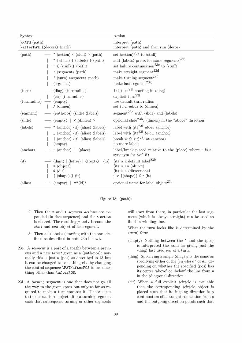
Syntax Action
\PATH 〈path〉 interpret 〈path〉\afterPATH{〈decor〉} 〈path〉 interpret 〈path〉 and then run 〈decor〉
〈path〉 −→ ~ 〈action〉 { 〈stuff〉 } 〈path〉 set 〈action〉23a to 〈stuff〉| ~ 〈which〉 { 〈labels〉 } 〈path〉 add 〈labels〉 prefix for some segments23b
| ~ { 〈stuff〉 } 〈path〉 set failure continuation23c to 〈stuff〉| ’ 〈segment〉 〈path〉 make straight segment23d
| ‘ 〈turn〉 〈segment〉 〈path〉 make turning segment23f
| 〈segment〉 make last segment23g
〈turn〉 −→ 〈diag〉 〈turnradius〉 1/4 turn23f starting in 〈diag〉| 〈cir〉 〈turnradius〉 explicit turn23f
〈turnradius〉 −→ 〈empty〉 use default turn radius| / 〈dimen〉 set turnradius to 〈dimen〉
〈segment〉 −→ 〈path-pos〉 〈slide〉 〈labels〉 segment23e with 〈slide〉 and 〈labels〉
〈slide〉 −→ 〈empty〉 | < 〈dimen〉 > optional slide23h: 〈dimen〉 in the “above” direction
〈labels〉 −→ ^ 〈anchor〉 〈it〉 〈alias〉 〈labels〉 label with 〈it〉23i above 〈anchor〉| _ 〈anchor〉 〈it〉 〈alias〉 〈labels〉 label with 〈it〉23i below 〈anchor〉| | 〈anchor〉 〈it〉 〈alias〉 〈labels〉 break with 〈it〉23j at 〈anchor〉| 〈empty〉 no more labels
〈anchor〉 −→ - 〈anchor〉 | 〈place〉 label/break placed relative to the 〈place〉 where - is asynonym for <>(.5)
〈it〉 −→ 〈digit〉 | 〈letter〉 | {〈text〉} | 〈cs〉 〈it〉 is a default label23k
| * 〈object〉 〈it〉 is an 〈object〉| @ 〈dir〉 〈it〉 is a 〈dir〉ectional| [ 〈shape〉 ] 〈it〉 use [〈shape〉] for 〈it〉
〈alias〉 −→ 〈empty〉 | ="〈id〉" optional name for label object23l
Figure 13: 〈path〉s
2. Then the = and < segment actions are ex-panded (in that sequence) and the < actionis cleared. The resulting p and c become thestart and end object of the segment.
3. Then all 〈labels〉 (starting with the ones de-fined as described in note 23b below).
23e. A segment is a part of a 〈path〉 between a previ-ous and a new target given as a 〈path-pos〉: nor-mally this is just a 〈pos〉 as described in §3 butit can be changed to something else by changingthe control sequence \PATHafterPOS to be some-thing other than \afterPOS.
23f. A turning segment is one that does not go allthe way to the given 〈pos〉 but only as far as re-quired to make a turn towards it. The c is setto the actual turn object after a turning segmentsuch that subsequent turning or other segments
will start from there, in particular the last seg-ment (which is always straight) can be used tofinish a winding line.
What the turn looks like is determined by the〈turn〉 form:
〈empty〉 Nothing between the ‘ and the 〈pos〉is interpreted the same as giving just the〈diag〉 last used out of a turn.
〈diag〉 Specifying a single 〈diag〉 d is the same asspecifying either of the 〈cir〉cles d^ or d_, de-pending on whether the specified 〈pos〉 hasits center ‘above’ or ‘below’ the line from pin the 〈diag〉onal direction.
〈cir〉 When a full explicit 〈cir〉cle is availablethen the corresponding 〈cir〉cle object isplaced such that its ingoing direction is acontinuation of a straight connection from pand the outgoing direction points such that
39
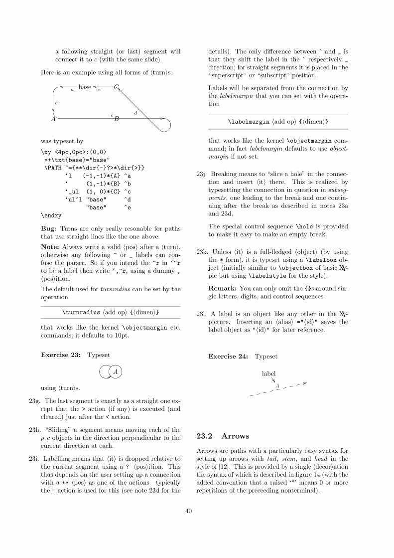
a following straight (or last) segment willconnect it to c (with the same slide).
Here is an example using all forms of 〈turn〉s:
base
A
GF oo a
B
@A�� bC
ABECD//c
E??????????????????
__
d
ooe
was typeset by
\xy <4pc,0pc>:(0,0)*+\txt{base}="base"\PATH ~={**\dir{-}?>*\dir{>}}
‘l (-1,-1)*{A} ^a‘ (1,-1)*{B} ^b‘_ul (1, 0)*{C} ^c‘ul^l "base" ^d
"base" ^e\endxy
Bug: Turns are only really resonable for pathsthat use straight lines like the one above.
Note: Always write a valid 〈pos〉 after a 〈turn〉,otherwise any following ^ or _ labels can con-fuse the parser. So if you intend the ^r in ‘^rto be a label then write ‘,^r, using a dummy ,〈pos〉ition.
The default used for turnradius can be set by theoperation
\turnradius 〈add op〉 {〈dimen〉}
that works like the kernel \objectmargin etc.commands; it defaults to 10pt.
Exercise 23: Typeset
A@GAFBECD@GAFBE99
using 〈turn〉s.
23g. The last segment is exactly as a straight one ex-cept that the > action (if any) is executed (andcleared) just after the < action.
23h. “Sliding” a segment means moving each of thep, c objects in the direction perpendicular to thecurrent direction at each.
23i. Labelling means that 〈it〉 is dropped relative tothe current segment using a ? 〈pos〉ition. Thisthus depends on the user setting up a connectionwith a ** 〈pos〉 as one of the actions—typicallythe = action is used for this (see note 23d for the
details). The only difference between ^ and _ isthat they shift the label in the ^ respectively _direction; for straight segments it is placed in the“superscript” or “subscript” position.
Labels will be separated from the connection bythe labelmargin that you can set with the opera-tion
\labelmargin 〈add op〉 {〈dimen〉}
that works like the kernel \objectmargin com-mand; in fact labelmargin defaults to use object-margin if not set.
23j. Breaking means to “slice a hole” in the connec-tion and insert 〈it〉 there. This is realized bytypesetting the connection in question in subseg-ments, one leading to the break and one contin-uing after the break as described in notes 23aand 23d.
The special control sequence \hole is providedto make it easy to make an empty break.
23k. Unless 〈it〉 is a full-fledged 〈object〉 (by usingthe * form), it is typeset using a \labelbox ob-ject (initially similar to \objectbox of basic XY-pic but using \labelstyle for the style).
Remark: You can only omit the {}s around sin-gle letters, digits, and control sequences.
23l. A label is an object like any other in the XY-picture. Inserting an 〈alias〉 ="〈id〉" saves thelabel object as "〈id〉" for later reference.
Exercise 24: Typeset
A33fffffffff
label��55
23.2 Arrows
Arrows are paths with a particularly easy syntax forsetting up arrows with tail , stem, and head in thestyle of [12]. This is provided by a single 〈decor〉ationthe syntax of which is described in figure 14 (with theadded convention that a raised ‘*’ means 0 or morerepetitions of the preceeding nonterminal).
40
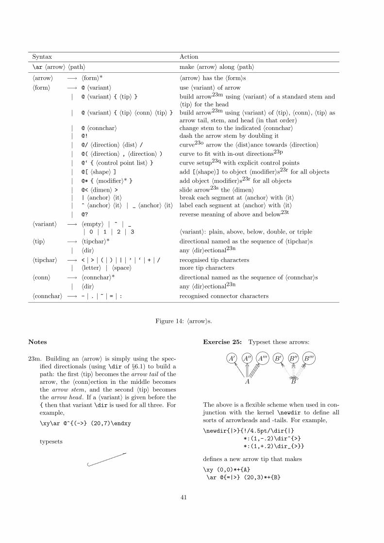
Syntax Action
\ar 〈arrow〉 〈path〉 make 〈arrow〉 along 〈path〉
〈arrow〉 −→ 〈form〉* 〈arrow〉 has the 〈form〉s〈form〉 −→ @ 〈variant〉 use 〈variant〉 of arrow
| @ 〈variant〉 { 〈tip〉 } build arrow23m using 〈variant〉 of a standard stem and〈tip〉 for the head
| @ 〈variant〉 { 〈tip〉 〈conn〉 〈tip〉 } build arrow23m using 〈variant〉 of 〈tip〉, 〈conn〉, 〈tip〉 asarrow tail, stem, and head (in that order)
| @ 〈connchar〉 change stem to the indicated 〈connchar〉| @! dash the arrow stem by doubling it| @/ 〈direction〉 〈dist〉 / curve23o arrow the 〈dist〉ance towards 〈direction〉| @( 〈direction〉 , 〈direction〉 ) curve to fit with in-out directions23p
| @‘ { 〈control point list〉 } curve setup23q with explicit control points| @[ 〈shape〉 ] add [〈shape〉] to object 〈modifier〉s23r for all objects| @* { 〈modifier〉* } add object 〈modifier〉s23r for all objects| @< 〈dimen〉 > slide arrow23s the 〈dimen〉| | 〈anchor〉 〈it〉 break each segment at 〈anchor〉 with 〈it〉| ^ 〈anchor〉 〈it〉 | _ 〈anchor〉 〈it〉 label each segment at 〈anchor〉 with 〈it〉| @? reverse meaning of above and below23t
〈variant〉 −→ 〈empty〉 | ^ | _| 0 | 1 | 2 | 3 〈variant〉: plain, above, below, double, or triple
〈tip〉 −→ 〈tipchar〉* directional named as the sequence of 〈tipchar〉s| 〈dir〉 any 〈dir〉ectional23n
〈tipchar〉 −→ < | > | ( | ) | | | ’ | ‘ | + | / recognised tip characters| 〈letter〉 | 〈space〉 more tip characters
〈conn〉 −→ 〈connchar〉* directional named as the sequence of 〈connchar〉s| 〈dir〉 any 〈dir〉ectional23n
〈connchar〉 −→ - | . | ~ | = | : recognised connector characters
Figure 14: 〈arrow〉s.
Notes
23m. Building an 〈arrow〉 is simply using the spec-ified directionals (using \dir of §6.1) to build apath: the first 〈tip〉 becomes the arrow tail of thearrow, the 〈conn〉ection in the middle becomesthe arrow stem, and the second 〈tip〉 becomesthe arrow head . If a 〈variant〉 is given before the{ then that variant \dir is used for all three. Forexample,
\xy\ar @^{(->} (20,7)\endxy
typesets
' �
5jjjjjjjjjjjjj
Exercise 25: Typeset these arrows:
A
A′8?9>:=;<ZZ444444
A′′8?9>:=;<KS A′′′@GAFBECD
<J
B
B′8?9>:=;<
tt
ZZZZB′′8?9>:=;<
____
KSKSB′′′@GAFBECD
JJJJ
<J<J
The above is a flexible scheme when used in con-junction with the kernel \newdir to define allsorts of arrowheads and -tails. For example,
\newdir{|>}{!/4.5pt/\dir{|}*:(1,-.2)\dir^{>}*:(1,+.2)\dir_{>}}
defines a new arrow tip that makes
\xy (0,0)*+{A}\ar @{=|>} (20,3)*+{B}
41
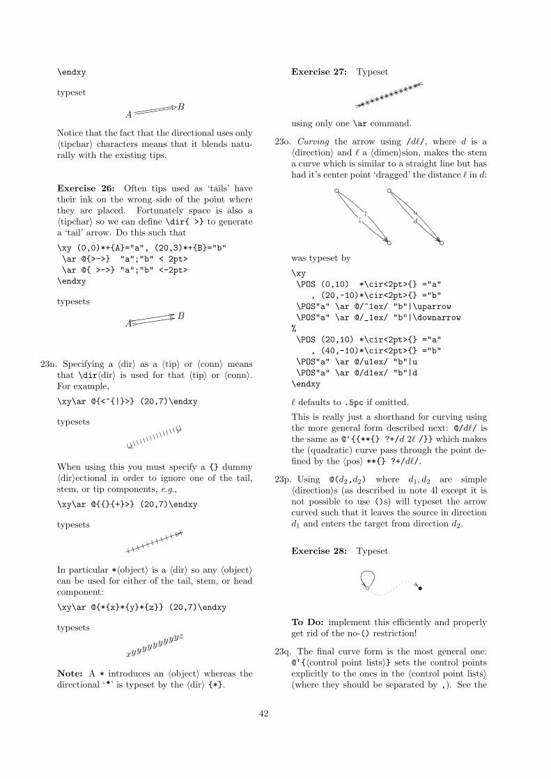
\endxy
typeset
AB$ .5ddddddddd ddddddddd
Notice that the fact that the directional uses only〈tipchar〉 characters means that it blends natu-rally with the existing tips.
Exercise 26: Often tips used as ‘tails’ havetheir ink on the wrong side of the point wherethey are placed. Fortunately space is also a〈tipchar〉 so we can define \dir{ >} to generatea ‘tail’ arrow. Do this such that
\xy (0,0)*+{A}="a", (20,3)*+{B}="b"\ar @{>->} "a";"b" < 2pt>\ar @{ >->} "a";"b" <-2pt>
\endxy
typesets
AB1111ddddddddd1111ddddddddd
23n. Specifying a 〈dir〉 as a 〈tip〉 or 〈conn〉 meansthat \dir〈dir〉 is used for that 〈tip〉 or 〈conn〉.For example,
\xy\ar @{<^{|}>} (20,7)\endxy
typesets
uu
55*****************
When using this you must specify a {} dummy〈dir〉ectional in order to ignore one of the tail,stem, or tip components, e.g.,
\xy\ar @{{}{+}>} (20,7)\endxy
typesets55*j*j*j*j*j*j*j*j*j*j*j*j
In particular *〈object〉 is a 〈dir〉 so any 〈object〉can be used for either of the tail, stem, or headcomponent:
\xy\ar @{*{x}*{y}*{z}} (20,7)\endxy
typesets
x
zyyyyyyyyy
Note: A * introduces an 〈object〉 whereas thedirectional ‘•’ is typeset by the 〈dir〉 {*}.
Exercise 27: Typeset
55 55
uuuuO�*jO�*jO�*jO�*jO�*jO�*jO�*jO�*jO�*jO�*jO�*jO�*j
using only one \ar command.
23o. Curving the arrow using /d`/, where d is a〈direction〉 and ` a 〈dimen〉sion, makes the stema curve which is similar to a straight line but hashad it’s center point ‘dragged’ the distance ` in d:
��� ��
��� ��↑
��
↓
$$
��� ��
��� ��
u
��
d
$$
was typeset by
\xy\POS (0,10) *\cir<2pt>{} ="a"
, (20,-10)*\cir<2pt>{} ="b"\POS"a" \ar @/^1ex/ "b"|\uparrow\POS"a" \ar @/_1ex/ "b"|\downarrow
%\POS (20,10) *\cir<2pt>{} ="a"
, (40,-10)*\cir<2pt>{} ="b"\POS"a" \ar @/u1ex/ "b"|u\POS"a" \ar @/d1ex/ "b"|d
\endxy
` defaults to .5pc if omitted.
This is really just a shorthand for curving usingthe more general form described next: @/d`/ isthe same as @‘{{**{} ?+/d 2` /}} which makesthe (quadratic) curve pass through the point de-fined by the 〈pos〉 **{} ?+/d`/.
23p. Using @(d2,d2) where d1, d2 are simple〈direction〉s (as described in note 4l except it isnot possible to use ()s) will typeset the arrowcurved such that it leaves the source in directiond1 and enters the target from direction d2.
Exercise 28: Typeset
◦�� •!!
To Do: implement this efficiently and properlyget rid of the no-() restriction!
23q. The final curve form is the most general one:@‘{〈control point lists〉} sets the control pointsexplicitly to the ones in the 〈control point lists〉(where they should be separated by ,). See the
42
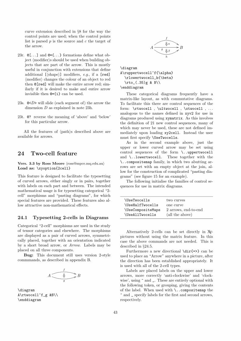
curve extension described in §8 for the way thecontrol points are used; when the control pointslist is parsed p is the source and c the target ofthe arrow.
23r. @[. . . ] and @*{. . . } formations define what ob-ject 〈modifier〉s should be used when building ob-jects that are part of the arrow. This is mostlyuseful in conjunction with extensions that defineadditional [〈shape〉] modifiers, e.g., if a [red]〈modifier〉 changes the colour of an object to redthen @[red] will make the entire arrow red; sim-ilarly if it is desired to make and entire arrowinvisible then @*{i} can be used.
23s. @<D> will slide (each segment of) the arrow thedimension D as explained in note 23h.
23t. @? reverse the meaning of ‘above’ and ‘below’for this particular arrow.
All the features of 〈path〉s described above areavailable for arrows.
24 Two-cell feature
Vers. 3.3 by Ross Moore 〈[email protected]〉Load as: \xyoption{2cell}
This feature is designed to facilitate the typesettingof curved arrows, either singly or in pairs, togetherwith labels on each part and between. The intendedmathematical usage is for typesetting categorical “2-cell” morphisms and “pasting diagrams”, for whichspecial features are provided. These features also al-low attractive non-mathematical effects.
24.1 Typesetting 2-cells in Diagrams
Categorical “2-cell” morphisms are used in the studyof tensor categories and elsewhere. The morphismsare displayed as a pair of curved arrows, symmetri-cally placed, together with an orientation indicatedby a short broad arrow, or Arrow. Labels may beplaced on all three components.
Bug: This document still uses version 2-stylecommmands, as described in appendix B.
A
f
))
g
55�� ���� B
\diagramA\rtwocell^f_g &B\\\enddiagram
A
f
##�� ���� α
;;
h
�� ���� β
g// B
\diagramA\ruppertwocell^f{\alpha}
\rlowertwocell_h{\beta}\rto_(.35)g & B\\
\enddiagram
These categorical diagrams frequently have amatrix-like layout, as with commutative diagrams.To facilitate this there are control sequences of theform: \rtwocell , \ultwocell , \xtwocell , . . .analogous to the names defined in xyv2 for use indiagrams produced using xymatrix. As this involvesthe definition of 21 new control sequences, many ofwhich may never be used, these are not defined im-mediately upon loading xy2cell. Instead the usermust first specify \UseTwocells.
As in the second example above, just theupper or lower curved arrow may be set usingcontrol sequences of the form \..uppertwocelland \..lowertwocell. These together with the\..compositemap family, in which two abutting ar-rows are set with an empty object at the join, al-low for the construction of complicated “pasting dia-grams” (see figure 15 for an example).
The following initialise the families of control se-quences for use in matrix diagrams.
\UseTwocells two curves\UseHalfTwocells one curve\UseCompositeMaps 2 arrows, end-to-end\UseAllTwocells (all the above)
Alternatively 2-cells can be set directly in XY-pictures without using the matrix feature. In thiscase the above commands are not needed. This isdescribed in §24.5.
Furthermore a new directional \dir{=>} can beused to place an “Arrow” anywhere in a picture, afterthe direction has been established appropriately. Itis used with all of the 2-cell types.
Labels are placed labels on the upper and lowerarrows, more correctly ‘anti-clockwise’ and ‘clock-wise’, using ^ and _. These are entirely optional withthe following token, or grouping, giving the contentsof the label. When used with \..compositemap the^ and _ specify labels for the first and second arrows,respectively.
43
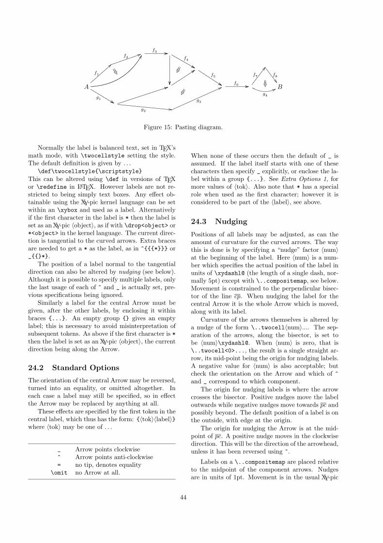
f3 ////
����
MMMMMMMMMf4
&&&& �
�����
JJJJJJJJJf5
%%%%A
{{{{{{{{{
f1
==
jjjjjjjjjjf2
55
2222��
FF
LLLLLLLLL
%%g1 %%
ttttttttt
9999
f6 //// 66g4
�� ����
�������
f7
CC
888888
f8��Biiiiiiiiiiiiiiiii
4444
\\\\\\\\\\\\\\\\\g2 --
mmmmmmmmmmmmmmmmmg3
66
Figure 15: Pasting diagram.
Normally the label is balanced text, set in TEX’smath mode, with \twocellstyle setting the style.The default definition is given by . . .
\def\twocellstyle{\scriptstyle}This can be altered using \def in versions of TEXor \redefine in LATEX. However labels are not re-stricted to being simply text boxes. Any effect ob-tainable using the XY-pic kernel language can be setwithin an \xybox and used as a label. Alternativelyif the first character in the label is * then the label isset as an XY-pic 〈object〉, as if with \drop<object> or*<object> in the kernel language. The current direc-tion is tangential to the curved arrows. Extra bracesare needed to get a * as the label, as in ^{{{*}}} or_{{}*}.
The position of a label normal to the tangentialdirection can also be altered by nudging (see below).Although it is possible to specify multiple labels, onlythe last usage of each of ^ and _ is actually set, pre-vious specifications being ignored.
Similarly a label for the central Arrow must begiven, after the other labels, by enclosing it withinbraces {...}. An empty group {} gives an emptylabel; this is necessary to avoid misinterpretation ofsubsequent tokens. As above if the first character is *then the label is set as an XY-pic 〈object〉, the currentdirection being along the Arrow.
24.2 Standard Options
The orientation of the central Arrow may be reversed,turned into an equality, or omitted altogether. Ineach case a label may still be specified, so in effectthe Arrow may be replaced by anything at all.
These effects are specified by the first token in thecentral label, which thus has the form: {〈tok〉〈label〉}where 〈tok〉 may be one of . . .
_ Arrow points clockwise^ Arrow points anti-clockwise= no tip, denotes equality
\omit no Arrow at all.
When none of these occurs then the default of _ isassumed. If the label itself starts with one of thesecharacters then specify _ explicitly, or enclose the la-bel within a group {...}. See Extra Options 1, formore values of 〈tok〉. Also note that * has a specialrole when used as the first character; however it isconsidered to be part of the 〈label〉, see above.
24.3 Nudging
Positions of all labels may be adjusted, as can theamount of curvature for the curved arrows. The waythis is done is by specifying a “nudge” factor 〈num〉at the beginning of the label. Here 〈num〉 is a num-ber which specifies the actual position of the label inunits of \xydashl@ (the length of a single dash, nor-mally 5pt) except with \..compositemap, see below.Movement is constrained to the perpendicular bisec-tor of the line cp. When nudging the label for thecentral Arrow it is the whole Arrow which is moved,along with its label.
Curvature of the arrows themselves is altered bya nudge of the form \..twocell〈num〉.... The sep-aration of the arrows, along the bisector, is set tobe 〈num〉\xydashl@. When 〈num〉 is zero, that is\..twocell<0>..., the result is a single straight ar-row, its mid-point being the origin for nudging labels.A negative value for 〈num〉 is also acceptable; butcheck the orientation on the Arrow and which of ^and _ correspond to which component.
The origin for nudging labels is where the arrowcrosses the bisector. Positive nudges move the labeloutwards while negative nudges move towards pc andpossibly beyond. The default position of a label is onthe outside, with edge at the origin.
The origin for nudging the Arrow is at the mid-point of pc. A positive nudge moves in the clockwisedirection. This will be the direction of the arrowhead,unless it has been reversed using ^.
Labels on a \..compositemap are placed relativeto the midpoint of the component arrows. Nudgesare in units of 1pt. Movement is in the usual XY-pic
44
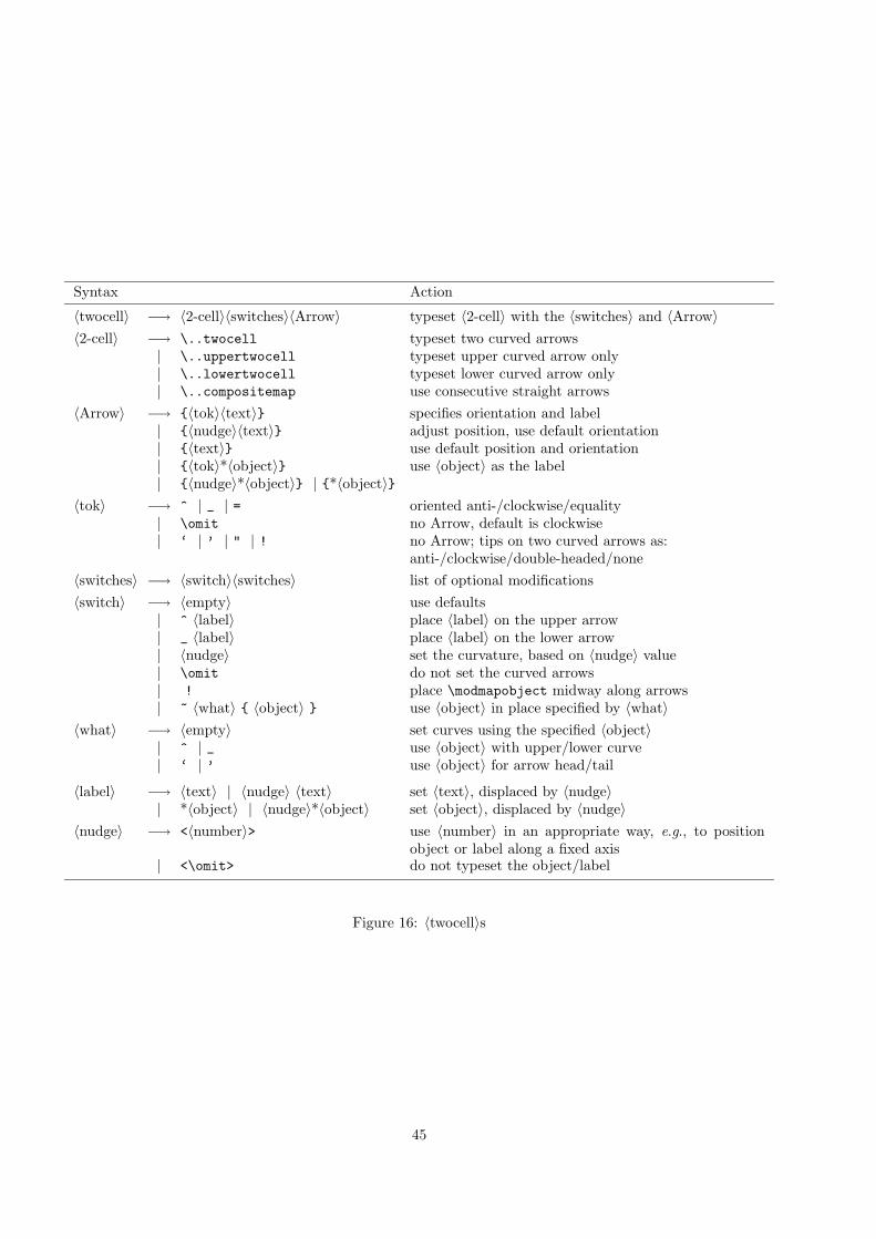
Syntax Action
〈twocell〉 −→ 〈2-cell〉〈switches〉〈Arrow〉 typeset 〈2-cell〉 with the 〈switches〉 and 〈Arrow〉〈2-cell〉 −→ \..twocell typeset two curved arrows
| \..uppertwocell typeset upper curved arrow only| \..lowertwocell typeset lower curved arrow only| \..compositemap use consecutive straight arrows
〈Arrow〉 −→ {〈tok〉〈text〉} specifies orientation and label| {〈nudge〉〈text〉} adjust position, use default orientation| {〈text〉} use default position and orientation| {〈tok〉*〈object〉} use 〈object〉 as the label| {〈nudge〉*〈object〉} | {*〈object〉}
〈tok〉 −→ ^ | _ | = oriented anti-/clockwise/equality| \omit no Arrow, default is clockwise| ‘ | ’ | " | ! no Arrow; tips on two curved arrows as:
anti-/clockwise/double-headed/none〈switches〉 −→ 〈switch〉〈switches〉 list of optional modifications〈switch〉 −→ 〈empty〉 use defaults
| ^ 〈label〉 place 〈label〉 on the upper arrow| _ 〈label〉 place 〈label〉 on the lower arrow| 〈nudge〉 set the curvature, based on 〈nudge〉 value| \omit do not set the curved arrows| ! place \modmapobject midway along arrows| ~ 〈what〉 { 〈object〉 } use 〈object〉 in place specified by 〈what〉
〈what〉 −→ 〈empty〉 set curves using the specified 〈object〉| ^ | _ use 〈object〉 with upper/lower curve| ‘ | ’ use 〈object〉 for arrow head/tail
〈label〉 −→ 〈text〉 | 〈nudge〉 〈text〉 set 〈text〉, displaced by 〈nudge〉| *〈object〉 | 〈nudge〉*〈object〉 set 〈object〉, displaced by 〈nudge〉
〈nudge〉 −→ <〈number〉> use 〈number〉 in an appropriate way, e.g., to positionobject or label along a fixed axis
| <\omit> do not typeset the object/label
Figure 16: 〈twocell〉s
45
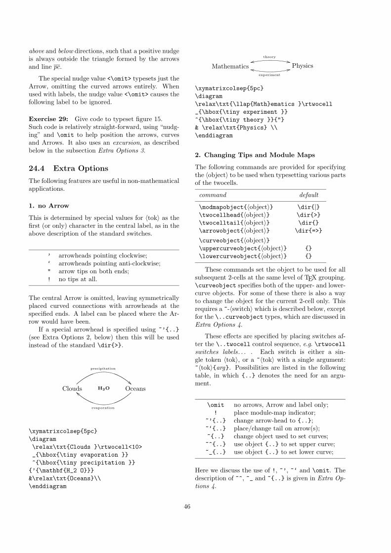
above and below directions, such that a positive nudgeis always outside the triangle formed by the arrowsand line pc.
The special nudge value <\omit> typesets just theArrow, omitting the curved arrows entirely. Whenused with labels, the nudge value <\omit> causes thefollowing label to be ignored.
Exercise 29: Give code to typeset figure 15.Such code is relatively straight-forward, using “nudg-ing” and \omit to help position the arrows, curvesand Arrows. It also uses an excursion, as describedbelow in the subsection Extra Options 3.
24.4 Extra Options
The following features are useful in non-mathematicalapplications.
1. no Arrow
This is determined by special values for 〈tok〉 as thefirst (or only) character in the central label, as in theabove description of the standard switches.
’ arrowheads pointing clockwise;‘ arrowheads pointing anti-clockwise;" arrow tips on both ends;! no tips at all.
The central Arrow is omitted, leaving symmetricallyplaced curved connections with arrowheads at thespecified ends. A label can be placed where the Ar-row would have been.
If a special arrowhead is specified using ~’{..}(see Extra Options 2, below) then this will be usedinstead of the standard \dir{>}.
Clouds
precipitation
!!
evaporation
aa H2O Oceans
\xymatrixcolsep{5pc}\diagram\relax\txt{Clouds }\rtwocell<10>_{\hbox{\tiny evaporation }}^{\hbox{\tiny precipitation }}
{’{\mathbf{H_2 O}}}&\relax\txt{Oceans}\\\enddiagram
Mathematics
theory,,rr
experiment
22ll Physics
\xymatrixcolsep{5pc}\diagram\relax\txt{\llap{Math}ematics }\rtwocell_{\hbox{\tiny experiment }}^{\hbox{\tiny theory }}{"}& \relax\txt{Physics} \\\enddiagram
2. Changing Tips and Module Maps
The following commands are provided for specifyingthe 〈object〉 to be used when typesetting various partsof the twocells.
command default
\modmapobject{〈object〉} \dir{|}\twocellhead{〈object〉} \dir{>}\twocelltail{〈object〉} \dir{}\arrowobject{〈object〉} \dir{=>}
\curveobject{〈object〉}\uppercurveobject{〈object〉} {}\lowercurveobject{〈object〉} {}
These commands set the object to be used for allsubsequent 2-cells at the same level of TEX grouping.\curveobject specifies both of the upper- and lower-curve objects. For some of these there is also a wayto change the object for the current 2-cell only. Thisrequires a ~-〈switch〉 which is described below, exceptfor the \..curveobject types, which are discussed inExtra Options 4.
These effects are specified by placing switches af-ter the \..twocell control sequence, e.g. \rtwocellswitches labels. . . . Each switch is either a sin-gle token 〈tok〉, or a ~〈tok〉 with a single argument:~〈tok〉{arg}. Possibilities are listed in the followingtable, in which {..} denotes the need for an argu-ment.
\omit no arrows, Arrow and label only;! place module-map indicator;
~’{..} change arrow-head to {..};~‘{..} place/change tail on arrow(s);~{..} change object used to set curves;~^{..} use object {..} to set upper curve;~_{..} use object {..} to set lower curve;
Here we discuss the use of !, ~’, ~‘ and \omit. Thedescription of ~^, ~_ and ~{..} is given in Extra Op-tions 4.
46
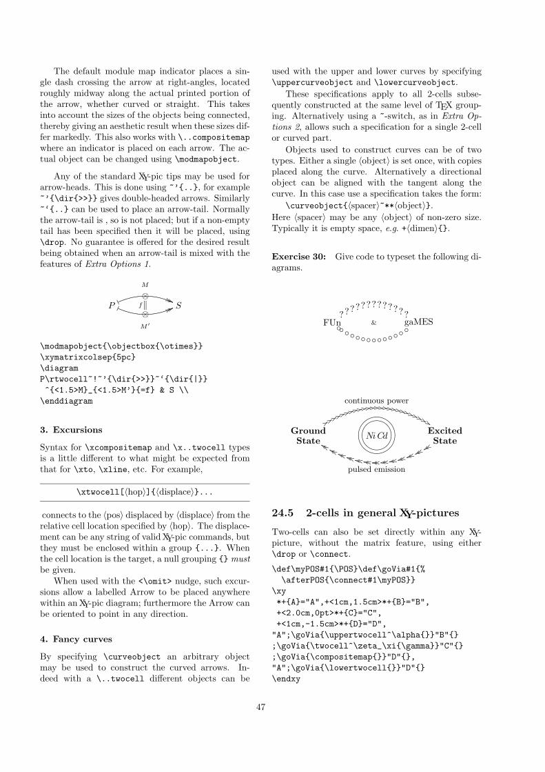
The default module map indicator places a sin-gle dash crossing the arrow at right-angles, locatedroughly midway along the actual printed portion ofthe arrow, whether curved or straight. This takesinto account the sizes of the objects being connected,thereby giving an aesthetic result when these sizes dif-fer markedly. This also works with \..compositemapwhere an indicator is placed on each arrow. The ac-tual object can be changed using \modmapobject.
Any of the standard XY-pic tips may be used forarrow-heads. This is done using ~’{..}, for example~’{\dir{>>}} gives double-headed arrows. Similarly~‘{..} can be used to place an arrow-tail. Normallythe arrow-tail is , so is not placed; but if a non-emptytail has been specified then it will be placed, using\drop. No guarantee is offered for the desired resultbeing obtained when an arrow-tail is mixed with thefeatures of Extra Options 1.
P⊗M
(( ((-
⊗M ′
66 66� f S
\modmapobject{\objectbox{\otimes}}\xymatrixcolsep{5pc}\diagramP\rtwocell~!~’{\dir{>>}}~‘{\dir{|}}^{<1.5>M}_{<1.5>M’}{=f} & S \\
\enddiagram
3. Excursions
Syntax for \xcompositemap and \x..twocell typesis a little different to what might be expected fromthat for \xto, \xline, etc. For example,
\xtwocell[〈hop〉]{〈displace〉}...
connects to the 〈pos〉 displaced by 〈displace〉 from therelative cell location specified by 〈hop〉. The displace-ment can be any string of valid XY-pic commands, butthey must be enclosed within a group {...}. Whenthe cell location is the target, a null grouping {} mustbe given.
When used with the <\omit> nudge, such excur-sions allow a labelled Arrow to be placed anywherewithin an XY-pic diagram; furthermore the Arrow canbe oriented to point in any direction.
4. Fancy curves
By specifying \curveobject an arbitrary objectmay be used to construct the curved arrows. In-deed with a \..twocell different objects can be
used with the upper and lower curves by specifying\uppercurveobject and \lowercurveobject.
These specifications apply to all 2-cells subse-quently constructed at the same level of TEX group-ing. Alternatively using a ~-switch, as in Extra Op-tions 2, allows such a specification for a single 2-cellor curved part.
Objects used to construct curves can be of twotypes. Either a single 〈object〉 is set once, with copiesplaced along the curve. Alternatively a directionalobject can be aligned with the tangent along thecurve. In this case use a specification takes the form:
\curveobject{〈spacer〉~**〈object〉}.Here 〈spacer〉 may be any 〈object〉 of non-zero size.Typically it is empty space, e.g. +〈dimen〉{}.
Exercise 30: Give code to typeset the following di-agrams.
FUn?????????????◦◦◦◦◦◦◦◦◦◦◦◦
◦◦& gaMES
GroundState
99 88 7766 55 55 4433 22 11 11 00 // .. -- -- ,, ++ ** )) )) (( '' && %%
continuous power
eeee gggg iiii jjjj llll mmmm oooo qqqq rrrr ttttuuuu wwwwyyyy
pulsed emission
NiCdgfed`abc_^]\XYZ[ ExcitedState
24.5 2-cells in general XY-pictures
Two-cells can also be set directly within any XY-picture, without the matrix feature, using either\drop or \connect.
\def\myPOS#1{\POS}\def\goVia#1{%\afterPOS{\connect#1\myPOS}}
\xy*+{A}="A",+<1cm,1.5cm>*+{B}="B",+<2.0cm,0pt>*+{C}="C",+<1cm,-1.5cm>*+{D}="D",
"A";\goVia{\uppertwocell^\alpha{}}"B"{};\goVia{\twocell^\zeta_\xi{\gamma}}"C"{};\goVia{\compositemap{}}"D"{},"A";\goVia{\lowertwocell{}}"D"{}\endxy
47
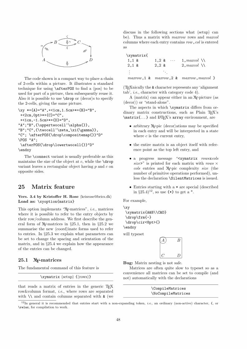
A
B C
D
α
11JJJJ !)
ζ((
ξ
66�� ���� γ RRRRR
((
� �� ��
��
ttttv~
88�� ����
The code shown is a compact way to place a chainof 2-cells within a picture. It illustrates a standardtechnique for using \afterPOS to find a 〈pos〉 to beused for part of a picture, then subsequently reuse it.Also it is possible to use \drop or 〈decor〉s to specifythe 2-cells, giving the same picture.
\xy *+{A}="A",+<1cm,1.5cm>*+{B}="B",+<2cm,0pt>*+{C}="C",+<1cm,-1.5cm>*+{D}="D",
"A";"B",{\uppertwocell^\alpha{}},"B";"C",{\twocell^\zeta_\xi{\gamma}},"C"; \afterPOS{\drop\compositemap{}}"D"\POS "A";\afterPOS{\drop\lowertwocell{}}"D"
\endxy
The \connect variant is usually preferable as thismaintains the size of the object at c, while the \dropvariant leaves a rectangular object having p and c onopposite sides.
25 Matrix feature
Vers. 3.4 by Kristoffer H. Rose 〈[email protected]〉Load as: \xyoption{matrix}
This option implements “XY-matrices”, i.e., matriceswhere it is possible to refer to the entry objects bytheir row/column address. We first describe the gen-eral form of XY-matrices in §25.1, then in §25.2 wesummarise the new 〈coord〉inate forms used to referto entries. In §25.3 we explain what parameters canbe set to change the spacing and orientation of thematrix, and in §25.4 we explain how the appearanceof the entries can be changed.
25.1 XY-matrices
The fundamental command of this feature is
\xymatrix 〈setup〉 {〈rows〉}
that reads a matrix of entries in the generic TEXrow&column format, i.e., where rows are separatedwith \\ and contain columns separated with & (we
discuss in the following sections what 〈setup〉 canbe). Thus a matrix with maxrow rows and maxcolcolumns where each entry contains row,col is enteredas
\xymatrix{1,1 & 1,2 & · · · 1,maxcol \\2,1 & 2,2 & 2,maxcol \\...
. . .maxrow,1 & maxrow,2 & maxrow,maxcol }
(TEXnically the & character represents any ‘alignmenttab’, i.e., character with category code 4).
A 〈matrix〉 can appear either in an XY-picture (as〈decor〉) or “stand-alone”.
The aspects in which \xymatrix differs from or-dinary matrix constructions, such as Plain TEX’s\matrix{. . . } and LATEX’s array environment, are
• arbitrary XY-pic 〈decor〉ations may be specifiedin each entry and will be interpreted in a statewhere c is the current entry,
• the entire matrix is an object itself with refer-ence point as the top left entry, and
• a progress message “<xymatrix rowsxcolssize>” is printed for each matrix with rows ×cols entries and XY-pic complexity size (thenumber of primitive operations performed), un-less the declaration \SilentMatrices is issued.
• Entries starting with a * are special (describedin §25.4)12, so use {*} to get a *.
For example,
\xy\xymatrix{A&B\\C&D}\drop\frm{-}\drop\cir<8pt>{}
\endxy
will typeset
A B
C D
8?9>:=;<
Bug: Matrix nesting is not safe.Matrices are often quite slow to typeset so as a
convenience all matrices can be set to compile (andnot) automatically with the declarations
\CompileMatrices\NoCompileMatrices
12In general it is recommended that entries start with a non-expanding token, i.e., an ordinary (non-active) character, {, or\relax, for compilation to work.
48
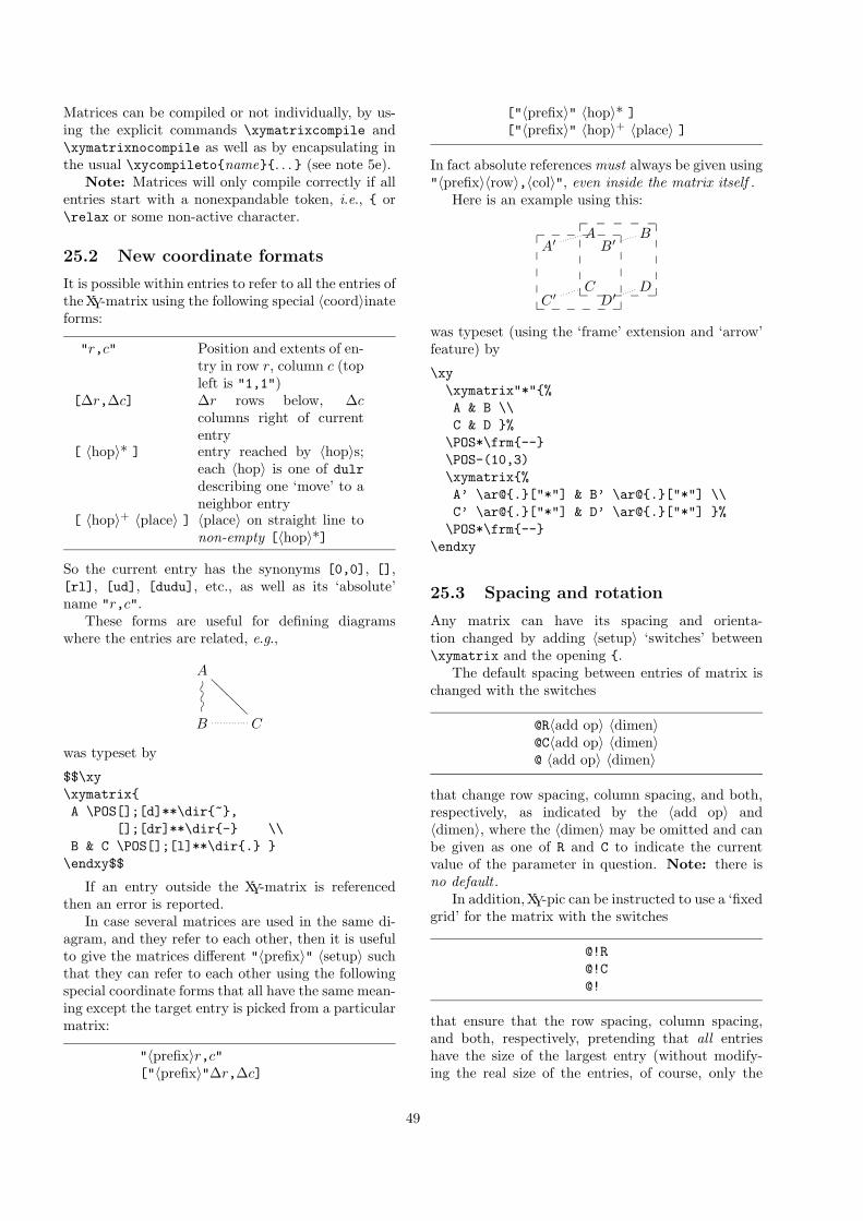
Matrices can be compiled or not individually, by us-ing the explicit commands \xymatrixcompile and\xymatrixnocompile as well as by encapsulating inthe usual \xycompileto{name}{. . . } (see note 5e).
Note: Matrices will only compile correctly if allentries start with a nonexpandable token, i.e., { or\relax or some non-active character.
25.2 New coordinate formats
It is possible within entries to refer to all the entries ofthe XY-matrix using the following special 〈coord〉inateforms:
"r,c" Position and extents of en-try in row r, column c (topleft is "1,1")
[∆r,∆c] ∆r rows below, ∆ccolumns right of currententry
[ 〈hop〉* ] entry reached by 〈hop〉s;each 〈hop〉 is one of dulrdescribing one ‘move’ to aneighbor entry
[ 〈hop〉+ 〈place〉 ] 〈place〉 on straight line tonon-empty [〈hop〉*]
So the current entry has the synonyms [0,0], [],[rl], [ud], [dudu], etc., as well as its ‘absolute’name "r,c".
These forms are useful for defining diagramswhere the entries are related, e.g.,
A
�O�O�O
@@@@@@@
B C
was typeset by
$$\xy\xymatrix{A \POS[];[d]**\dir{~},
[];[dr]**\dir{-} \\B & C \POS[];[l]**\dir{.} }
\endxy$$
If an entry outside the XY-matrix is referencedthen an error is reported.
In case several matrices are used in the same di-agram, and they refer to each other, then it is usefulto give the matrices different "〈prefix〉" 〈setup〉 suchthat they can refer to each other using the followingspecial coordinate forms that all have the same mean-ing except the target entry is picked from a particularmatrix:
"〈prefix〉r,c"["〈prefix〉"∆r,∆c]
["〈prefix〉" 〈hop〉* ]["〈prefix〉" 〈hop〉+ 〈place〉 ]
In fact absolute references must always be given using"〈prefix〉〈row〉,〈col〉", even inside the matrix itself .
Here is an example using this:
A B
C D
_ _ _ _ _�����
�����
_ _ _ _ _
A′ B′
C ′ D′
_ _ _ _ _ _�����
�����
_ _ _ _ _ _
was typeset (using the ‘frame’ extension and ‘arrow’feature) by
\xy\xymatrix"*"{%A & B \\C & D }%
\POS*\frm{--}\POS-(10,3)\xymatrix{%A’ \ar@{.}["*"] & B’ \ar@{.}["*"] \\C’ \ar@{.}["*"] & D’ \ar@{.}["*"] }%
\POS*\frm{--}\endxy
25.3 Spacing and rotation
Any matrix can have its spacing and orienta-tion changed by adding 〈setup〉 ‘switches’ between\xymatrix and the opening {.
The default spacing between entries of matrix ischanged with the switches
@R〈add op〉 〈dimen〉@C〈add op〉 〈dimen〉@ 〈add op〉 〈dimen〉
that change row spacing, column spacing, and both,respectively, as indicated by the 〈add op〉 and〈dimen〉, where the 〈dimen〉 may be omitted and canbe given as one of R and C to indicate the currentvalue of the parameter in question. Note: there isno default .
In addition, XY-pic can be instructed to use a ‘fixedgrid’ for the matrix with the switches
@!R@!C@!
that ensure that the row spacing, column spacing,and both, respectively, pretending that all entrieshave the size of the largest entry (without modify-ing the real size of the entries, of course, only the
49
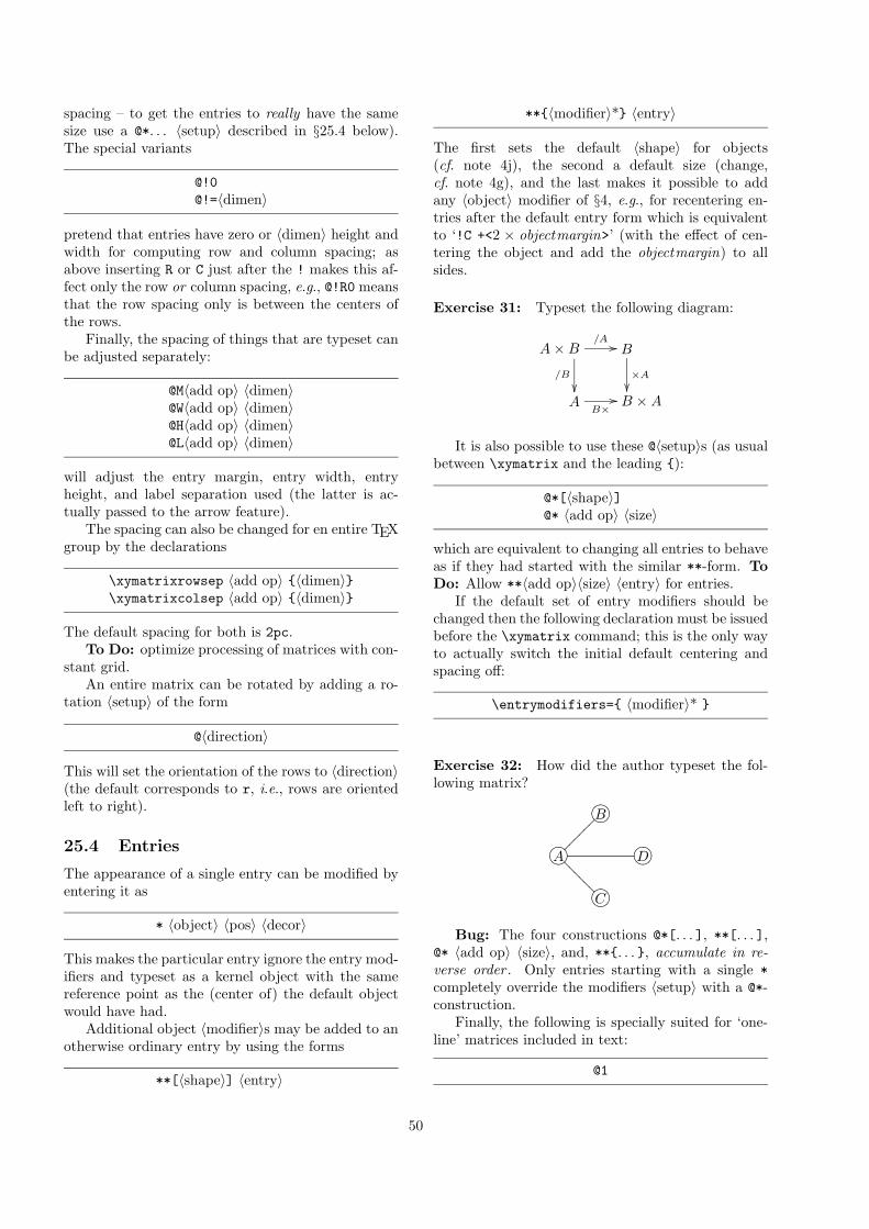
spacing – to get the entries to really have the samesize use a @*. . . 〈setup〉 described in §25.4 below).The special variants
@!0@!=〈dimen〉
pretend that entries have zero or 〈dimen〉 height andwidth for computing row and column spacing; asabove inserting R or C just after the ! makes this af-fect only the row or column spacing, e.g., @!R0 meansthat the row spacing only is between the centers ofthe rows.
Finally, the spacing of things that are typeset canbe adjusted separately:
@M〈add op〉 〈dimen〉@W〈add op〉 〈dimen〉@H〈add op〉 〈dimen〉@L〈add op〉 〈dimen〉
will adjust the entry margin, entry width, entryheight, and label separation used (the latter is ac-tually passed to the arrow feature).
The spacing can also be changed for en entire TEXgroup by the declarations
\xymatrixrowsep 〈add op〉 {〈dimen〉}\xymatrixcolsep 〈add op〉 {〈dimen〉}
The default spacing for both is 2pc.To Do: optimize processing of matrices with con-
stant grid.An entire matrix can be rotated by adding a ro-
tation 〈setup〉 of the form
@〈direction〉
This will set the orientation of the rows to 〈direction〉(the default corresponds to r, i.e., rows are orientedleft to right).
25.4 Entries
The appearance of a single entry can be modified byentering it as
* 〈object〉 〈pos〉 〈decor〉
This makes the particular entry ignore the entry mod-ifiers and typeset as a kernel object with the samereference point as the (center of) the default objectwould have had.
Additional object 〈modifier〉s may be added to anotherwise ordinary entry by using the forms
**[〈shape〉] 〈entry〉
**{〈modifier〉*} 〈entry〉
The first sets the default 〈shape〉 for objects(cf. note 4j), the second a default size (change,cf. note 4g), and the last makes it possible to addany 〈object〉 modifier of §4, e.g., for recentering en-tries after the default entry form which is equivalentto ‘!C +<2 × objectmargin>’ (with the effect of cen-tering the object and add the objectmargin) to allsides.
Exercise 31: Typeset the following diagram:
A×B/A //
/B
��
B
×A��
AB×// B ×A
It is also possible to use these @〈setup〉s (as usualbetween \xymatrix and the leading {):
@*[〈shape〉]@* 〈add op〉 〈size〉
which are equivalent to changing all entries to behaveas if they had started with the similar **-form. ToDo: Allow **〈add op〉〈size〉 〈entry〉 for entries.
If the default set of entry modifiers should bechanged then the following declaration must be issuedbefore the \xymatrix command; this is the only wayto actually switch the initial default centering andspacing off:
\entrymodifiers={ 〈modifier〉* }
Exercise 32: How did the author typeset the fol-lowing matrix?
/.-,()*+A������
??????
/.-,()*+B
/.-,()*+C
/.-,()*+D
Bug: The four constructions @*[. . . ], **[. . . ],@* 〈add op〉 〈size〉, and, **{. . . }, accumulate in re-verse order . Only entries starting with a single *completely override the modifiers 〈setup〉 with a @*-construction.
Finally, the following is specially suited for ‘one-line’ matrices included in text:
@1
50
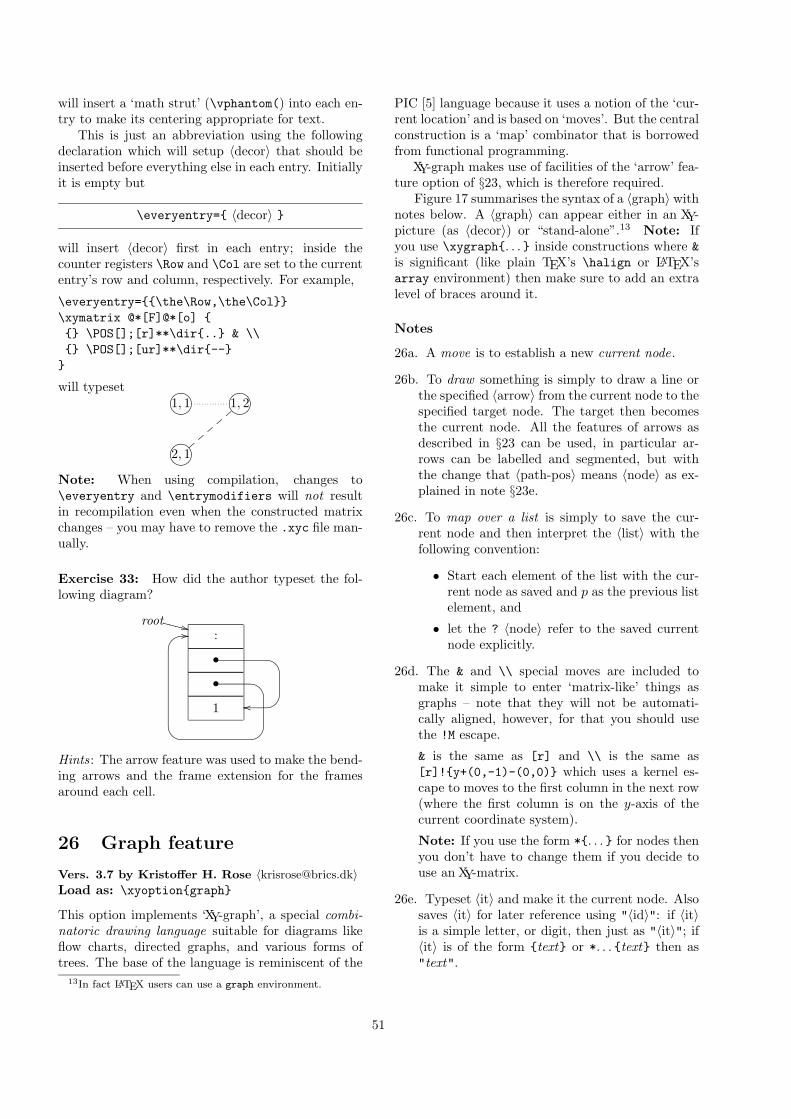
will insert a ‘math strut’ (\vphantom() into each en-try to make its centering appropriate for text.
This is just an abbreviation using the followingdeclaration which will setup 〈decor〉 that should beinserted before everything else in each entry. Initiallyit is empty but
\everyentry={ 〈decor〉 }
will insert 〈decor〉 first in each entry; inside thecounter registers \Row and \Col are set to the currententry’s row and column, respectively. For example,
\everyentry={{\the\Row,\the\Col}}\xymatrix @*[F]@*[o] {{} \POS[];[r]**\dir{..} & \\{} \POS[];[ur]**\dir{--}
}
will typeset ?>=<89:;1, 1 ?>=<89:;1, 2
?>=<89:;2, 1
{{
{{
{
Note: When using compilation, changes to\everyentry and \entrymodifiers will not resultin recompilation even when the constructed matrixchanges – you may have to remove the .xyc file man-ually.
Exercise 33: How did the author typeset the fol-lowing diagram?
:root ++WWWW
• EDBC
oo
• EDBC@A
GF //
1
Hints: The arrow feature was used to make the bend-ing arrows and the frame extension for the framesaround each cell.
26 Graph feature
Vers. 3.7 by Kristoffer H. Rose 〈[email protected]〉Load as: \xyoption{graph}
This option implements ‘XY-graph’, a special combi-natoric drawing language suitable for diagrams likeflow charts, directed graphs, and various forms oftrees. The base of the language is reminiscent of the
PIC [5] language because it uses a notion of the ‘cur-rent location’ and is based on ‘moves’. But the centralconstruction is a ‘map’ combinator that is borrowedfrom functional programming.
XY-graph makes use of facilities of the ‘arrow’ fea-ture option of §23, which is therefore required.
Figure 17 summarises the syntax of a 〈graph〉 withnotes below. A 〈graph〉 can appear either in an XY-picture (as 〈decor〉) or “stand-alone”.13 Note: Ifyou use \xygraph{. . . } inside constructions where &is significant (like plain TEX’s \halign or LATEX’sarray environment) then make sure to add an extralevel of braces around it.
Notes
26a. A move is to establish a new current node.
26b. To draw something is simply to draw a line orthe specified 〈arrow〉 from the current node to thespecified target node. The target then becomesthe current node. All the features of arrows asdescribed in §23 can be used, in particular ar-rows can be labelled and segmented, but withthe change that 〈path-pos〉 means 〈node〉 as ex-plained in note §23e.
26c. To map over a list is simply to save the cur-rent node and then interpret the 〈list〉 with thefollowing convention:
• Start each element of the list with the cur-rent node as saved and p as the previous listelement, and
• let the ? 〈node〉 refer to the saved currentnode explicitly.
26d. The & and \\ special moves are included tomake it simple to enter ‘matrix-like’ things asgraphs – note that they will not be automati-cally aligned, however, for that you should usethe !M escape.
& is the same as [r] and \\ is the same as[r]!{y+(0,-1)-(0,0)} which uses a kernel es-cape to moves to the first column in the next row(where the first column is on the y-axis of thecurrent coordinate system).
Note: If you use the form *{. . . } for nodes thenyou don’t have to change them if you decide touse an XY-matrix.
26e. Typeset 〈it〉 and make it the current node. Alsosaves 〈it〉 for later reference using "〈id〉": if 〈it〉is a simple letter, or digit, then just as "〈it〉"; if〈it〉 is of the form {text} or *. . . {text} then as"text".
13In fact LATEX users can use a graph environment.
51
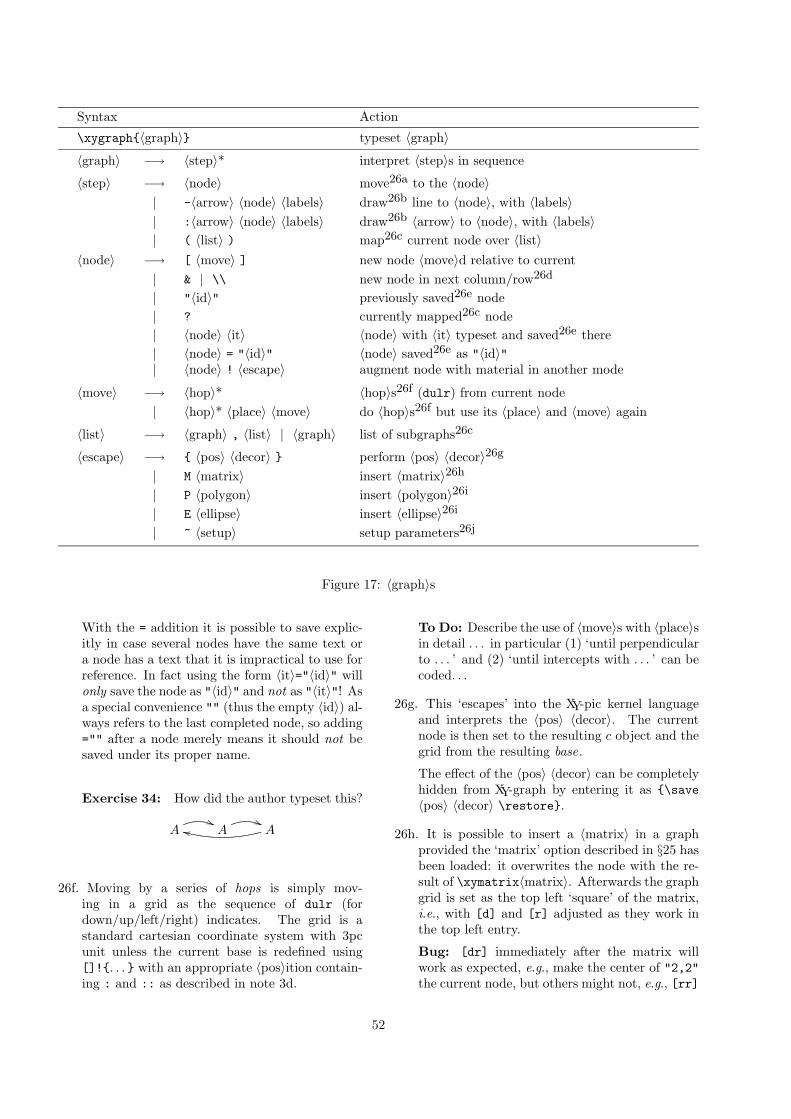
Syntax Action
\xygraph{〈graph〉} typeset 〈graph〉
〈graph〉 −→ 〈step〉* interpret 〈step〉s in sequence
〈step〉 −→ 〈node〉 move26a to the 〈node〉| -〈arrow〉 〈node〉 〈labels〉 draw26b line to 〈node〉, with 〈labels〉| :〈arrow〉 〈node〉 〈labels〉 draw26b 〈arrow〉 to 〈node〉, with 〈labels〉| ( 〈list〉 ) map26c current node over 〈list〉
〈node〉 −→ [ 〈move〉 ] new node 〈move〉d relative to current| & | \\ new node in next column/row26d
| "〈id〉" previously saved26e node| ? currently mapped26c node| 〈node〉 〈it〉 〈node〉 with 〈it〉 typeset and saved26e there| 〈node〉 = "〈id〉" 〈node〉 saved26e as "〈id〉"| 〈node〉 ! 〈escape〉 augment node with material in another mode
〈move〉 −→ 〈hop〉* 〈hop〉s26f (dulr) from current node| 〈hop〉* 〈place〉 〈move〉 do 〈hop〉s26f but use its 〈place〉 and 〈move〉 again
〈list〉 −→ 〈graph〉 , 〈list〉 | 〈graph〉 list of subgraphs26c
〈escape〉 −→ { 〈pos〉 〈decor〉 } perform 〈pos〉 〈decor〉26g
| M 〈matrix〉 insert 〈matrix〉26h
| P 〈polygon〉 insert 〈polygon〉26i
| E 〈ellipse〉 insert 〈ellipse〉26i
| ~ 〈setup〉 setup parameters26j
Figure 17: 〈graph〉s
With the = addition it is possible to save explic-itly in case several nodes have the same text ora node has a text that it is impractical to use forreference. In fact using the form 〈it〉="〈id〉" willonly save the node as "〈id〉" and not as "〈it〉"! Asa special convenience "" (thus the empty 〈id〉) al-ways refers to the last completed node, so adding="" after a node merely means it should not besaved under its proper name.
Exercise 34: How did the author typeset this?
A A((
A((
kk
26f. Moving by a series of hops is simply mov-ing in a grid as the sequence of dulr (fordown/up/left/right) indicates. The grid is astandard cartesian coordinate system with 3pcunit unless the current base is redefined using[]!{. . . } with an appropriate 〈pos〉ition contain-ing : and :: as described in note 3d.
To Do: Describe the use of 〈move〉s with 〈place〉sin detail . . . in particular (1) ‘until perpendicularto . . . ’ and (2) ‘until intercepts with . . . ’ can becoded. . .
26g. This ‘escapes’ into the XY-pic kernel languageand interprets the 〈pos〉 〈decor〉. The currentnode is then set to the resulting c object and thegrid from the resulting base.
The effect of the 〈pos〉 〈decor〉 can be completelyhidden from XY-graph by entering it as {\save〈pos〉 〈decor〉 \restore}.
26h. It is possible to insert a 〈matrix〉 in a graphprovided the ‘matrix’ option described in §25 hasbeen loaded: it overwrites the node with the re-sult of \xymatrix〈matrix〉. Afterwards the graphgrid is set as the top left ‘square’ of the matrix,i.e., with [d] and [r] adjusted as they work inthe top left entry.
Bug: [dr] immediately after the matrix willwork as expected, e.g., make the center of "2,2"the current node, but others might not, e.g., [rr]
52
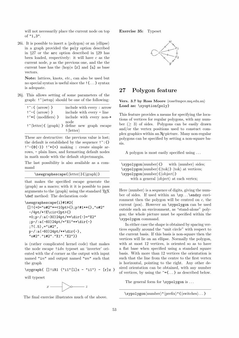
will not necessarily place the current node on topof "1,3".
26i. It is possible to insert a 〈polygon〉 or an 〈ellipse〉in a graph provided the poly option describedin §27 or the arc option described in §29 hasbeen loaded, respectively: it will have c as thecurrent node, p as the previous one, and the thecurrent base has the 〈hop〉s [r] and [u] as basevectors.Note: lattices, knots, etc., can also be used butno special syntax is useful since the !{. . . } syntaxis adequate.
26j. This allows setting of some parameters of thegraph: !~〈setup〉 should be one of the following:
!~:{ 〈arrow〉 } include with every : arrow!~-{ 〈arrow〉 } include with every - line!~*{ 〈modifiers〉 } include with every non-*
node!~〈letter〉{ 〈graph〉 } define new graph escape
!〈letter〉
These are destructive: the previous value is lost;the default is established by the sequence !~:{}!~-{@{-}} !~*{+} making : create simple ar-rows, - plain lines, and formatting default nodesin math mode with the default objectmargin.The last possibility is also available as a com-mand
\newgraphescape{〈letter〉}{〈graph〉}
that makes the specified escape generate the〈graph〉 as a macro; with it it is possible to passarguments to the 〈graph〉 using the standard TEX\def method: The declaration code
\newgraphescape{i}#1#2{[]!{+0="o#2"*=<10pt>{};p!#1**{},"o#2"-/4pt/*!E\cir<2pt>{}+0;p-/:a(-30)24pt/**\dir{-}="X2";p-/:a(-60)24pt/="X1"**\dir{-};?(.5),="i#2",p-/:a(-60)24pt/**\dir{-},"o#2"."i#2"."X1"."X2"}}
is (rather complicated kernel code) that makesthe node escape !idn typeset an ‘inverter’ ori-ented with the d corner as the output with inputnamed "in" and output named "on" such thatthe graph
\xygraph{ []!iR1 ("i1"[l]x - "i1") - [r]z }
will typeset
��� ��MMMMMqqqqq
x z
The final exercise illustrates much of the above.
Exercise 35: Typeset
w
x1
��??
??
z
������
����
y
��????
??? x2??��
��
OOssgggg
ggggOO
++WWWWWWWW
27 Polygon feature
Vers. 3.7 by Ross Moore 〈[email protected]〉Load as: \xyoption{poly}
This feature provides a means for specifying the loca-tions of vertices for regular polygons, with any num-ber (≥ 3) of sides. Polygons can be easily drawnand/or the vertex positions used to constuct com-plex graphics within an XY-picture. Many non-regularpolygons can be specified by setting a non-square ba-sis.
A polygon is most easily specified using . . .
\xypolygon〈number〉{} with 〈number〉 sides;\xypolygon〈number〉{〈tok〉} 〈tok〉 at vertices;\xypolygon〈number〉{〈object〉}
with a general 〈object〉 at each vertex;
Here 〈number〉 is a sequence of digits, giving the num-ber of sides. If used within an \xy. . . \endxy envi-ronment then the polygon will be centred on c, thecurrent 〈pos〉. However an \xypolygon can be usedoutside such an environment, as “stand-alone” poly-gon; the whole picture must be specified within the\xypolygon command.
In either case the shape is obtained by spacing ver-tices equally around the “unit circle” with respect tothe current basis. If this basis is non-square then thevertices will lie on an ellipse. Normally the polygon,with at most 12 vertices, is oriented so as to havea flat base when specified using a standard squarebasis. With more than 12 vertices the orientation issuch that the line from the centre to the first vertexis horizontal, pointing to the right. Any other de-sired orientation can be obtained, with any numberof vertices, by using the ~={. . . } as described below.
The general form for \xypolygon is . . .
\xypolygon〈number〉"〈prefix〉"{〈switches〉. . . }
53
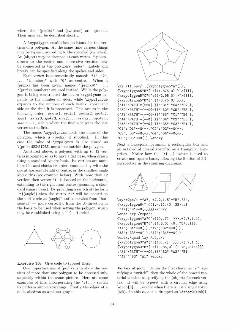
where the "〈prefix〉" and 〈switches〉 are optional.Their uses will be described shortly.
A \xypolygon establishes positions for the ver-tices of a polygon. At the same time various thingsmay be typeset, according to the specified 〈switches〉.An 〈object〉 may be dropped at each vertex, “spokes”drawn to the centre and successive vertices maybe connected as the polygon’s “sides”. Labels andbreaks can be specified along the spokes and sides.
Each vertex is automatically named: "1", "2",. . . , "〈number〉" with "0" as centre. When a〈prefix〉 has been given, names "〈prefix〉0", . . . ,"〈prefix〉〈number〉" are used instead. While the poly-gon is being constructed the macro \xypolynum ex-pands to the number of sides, while \xypolynodeexpands to the number of each vertex, spoke andside at the time it is processed. This occurs in thefollowing order: vertex 1, spoke 1, vertex 2, spoke 2,side 1, vertex 3, spoke 3, side 2, . . . , vertex n, spoke n,side n − 1, side n where the final side joins the lastvertex to the first.
The macro \xypolyname holds the name of thepolygon, which is 〈prefix〉 if supplied. In thiscase the value of \xypolynum is also stored as\〈prefix〉NUMSIDES, accessible outside the polygon.
As stated above, a polygon with up to 12 ver-tices is oriented so as to have a flat base, when drawnusing a standard square basis. Its vertices are num-bered in anti-clockwise order, commencing with theone at horizontal-right of centre, or the smallest angleabove this (see example below). With more than 12vertices then vertex "1" is located on the horizontal,extending to the right from centre (assuming a stan-dard square basis). By providing a switch of the form~={〈angle〉} then the vertex "1" will be located onthe unit circle at 〈angle〉◦ anti-clockwise from “hor-izontal” — more correctly, from the X-direction inthe basis to be used when setting the polygon, whichmay be established using a ~:{. . . } switch.
•
•
•
111111111
1
2 3
0 '!&"%#$ '!&"%#$ '!&"%#$
111 '!&"%#$111 '!&"%#$
'!&"%#$ 111
'!&"%#$111
1
23
4
5 6
01
2113 SS
4kk
5
6
%%
7
DD8
9zz
��
Exercise 36: Give code to typeset these.One important use of 〈prefix〉 is to allow the ver-
tices of more than one polygon to be accessed sub-sequently within the same picture. Here are someexamples of this, incorporating the ~:{. . . } switchto perform simple rescalings. Firstly the edges of adodecahedron as a planar graph:
HHHHH vvvvv
)))))�����
HHHHHHHHHHHHHHHHvvvvvvvvvvvvvvvv
)))))))))))))))) ����������������
iiii
hhhhhhh VVVVVVV
�������
UUUU
TTTTTTT����
8888888�������
6666jjjjjjj
5555555 iiiUUU
��� 666
\xy /l1.5pc/:,{\xypolygon5"A"{}},{\xypolygon5"B"{~:{(1.875,0):}~>{}}},{\xypolygon5"C"{~:{(-2.95,0):}~>{}}},{\xypolygon5"D"{~:{(-3.75,0):}}},{"A1"\PATH~={**@{-}}’"B1"’"C4"’"B2"},{"A2"\PATH~={**@{-}}’"B2"’"C5"’"B3"},{"A3"\PATH~={**@{-}}’"B3"’"C1"’"B4"},{"A4"\PATH~={**@{-}}’"B4"’"C2"’"B5"},{"A5"\PATH~={**@{-}}’"B5"’"C3"’"B1"},"C1";"D1"**@{-},"C2";"D2"**@{-},"C3";"D3"**@{-},"C4";"D4"**@{-},"C5";"D5"**@{-} \endxy
Next a hexagonal pyramid, a rectangular box andan octahedral crystal specified as a triangular anti-prism. Notice how the ~:{. . . } switch is used tocreate non-square bases, allowing the illusion of 3D-perspective in the resulting diagrams:
/////////
'''''''HHH
\\\\\
���������mmm
���������HHH
$$$$$$$$$\\\\\ mmm �������9999999
������<<<<<<<
\xy/r2pc/: ="A", +(.2,1.5)="B","A",{\xypolygon6{~:{(1,-.1):(0,.33)::}~<>{;"B"**@{-}}}}\endxy
\quad \xy /r2pc/:{\xypolygon4"A"{~:{(0,.7)::}}},+(.7,1.1),{\xypolygon4"B"{~:{(.8,0):(0,.75)::}}},"A1";"B1"**@{.},"A2";"B2"**@{.},"A3";"B3"**@{.},"A4";"B4"**@{.}\endxy\quad \xy /r2pc/:{\xypolygon3"A"{~:{(0,.7)::}}},+(.7,1.1),{\xypolygon3"B"{~:{(-.85,0):(-.15,.8)::}}},"A1"\PATH~={**@{.}}’"B2"’"A3"’"B1"’"A2"’"B3"’"A1" \endxy
Vertex object: Unless the first character is ~, sig-nifying a “switch”, then the whole of the braced ma-terial is taken as specifying the 〈object〉 for each ver-tex. It will be typeset with a circular edge using\drop[o]..., except when there is just a single token〈tok〉. In this case it is dropped as \drop=0{〈tok〉},
54
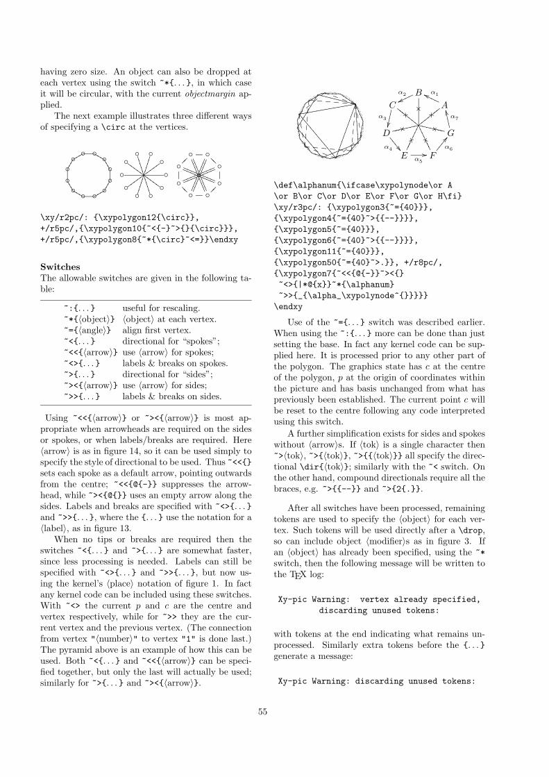
having zero size. An object can also be dropped ateach vertex using the switch ~*{. . . }, in which caseit will be circular, with the current objectmargin ap-plied.
The next example illustrates three different waysof specifying a \circ at the vertices.
◦◦111
◦MMM◦◦qqq
◦
◦◦1
11
◦MMM◦ ◦qqq
◦
◦◦vvvvv
◦�����
◦)))))◦HHHHH◦◦vvvvv
◦�����
◦)))))
◦HHHHH◦llll llll
◦����
����
??◦,,,,
,,,,◦ RRRRRRRR
��
◦ llllllll
◦��������
??◦
,,,,
,,,,◦
RRRRRRRR
��
\xy/r2pc/: {\xypolygon12{\circ}},+/r5pc/,{\xypolygon10{~<{-}~>{}{\circ}}},+/r5pc/,{\xypolygon8{~*{\circ}~<=}}\endxy
SwitchesThe allowable switches are given in the following ta-ble:
~:{. . . } useful for rescaling.~*{〈object〉} 〈object〉 at each vertex.~={〈angle〉} align first vertex.~<{. . . } directional for “spokes”;~<<{〈arrow〉} use 〈arrow〉 for spokes;~<>{. . . } labels & breaks on spokes.~>{. . . } directional for “sides”;~><{〈arrow〉} use 〈arrow〉 for sides;~>>{. . . } labels & breaks on sides.
Using ~<<{〈arrow〉} or ~><{〈arrow〉} is most ap-propriate when arrowheads are required on the sidesor spokes, or when labels/breaks are required. Here〈arrow〉 is as in figure 14, so it can be used simply tospecify the style of directional to be used. Thus ~<<{}sets each spoke as a default arrow, pointing outwardsfrom the centre; ~<<{@{-}} suppresses the arrow-head, while ~><{@{}} uses an empty arrow along thesides. Labels and breaks are specified with ~<>{. . . }and ~>>{. . . }, where the {. . . } use the notation for a〈label〉, as in figure 13.
When no tips or breaks are required then theswitches ~<{. . . } and ~>{. . . } are somewhat faster,since less processing is needed. Labels can still bespecified with ~<>{. . . } and ~>>{. . . }, but now us-ing the kernel’s 〈place〉 notation of figure 1. In factany kernel code can be included using these switches.With ~<> the current p and c are the centre andvertex respectively, while for ~>> they are the cur-rent vertex and the previous vertex. (The connectionfrom vertex "〈number〉" to vertex "1" is done last.)The pyramid above is an example of how this can beused. Both ~<{. . . } and ~<<{〈arrow〉} can be speci-fied together, but only the last will actually be used;similarly for ~>{. . . } and ~><{〈arrow〉}.
eeeeeeeeeeeee
:::::::::::::�������������
\ \ \ \ \ \
��
��
��
\\\\\\
��
��
��
WWWWWWWWW
���������
:::::::::
lllllllll
!!!!!!!!!
S S S Sz
zz
z
%%
%%
SSSSz
zz
z
%%
%%
JJJJJ_____
sssss
�����
#####
:::::
UUUUU hhhhh
�����
�����
-----A
\�yyyy
yyy
B
�?
α1ggPPPPC
"bEEEE
EEE
α2wwnnnn
DK�ffff
fff
α3
������
E
k+����
���α4 ��9999
F
�S....
...
α5
//
G4tXXXX
XXX
α6
BB����
α7
SS&&&&
\def\alphanum{\ifcase\xypolynode\or A\or B\or C\or D\or E\or F\or G\or H\fi}\xy/r3pc/: {\xypolygon3{~={40}}},{\xypolygon4{~={40}~>{{--}}}},{\xypolygon5{~={40}}},{\xypolygon6{~={40}~>{{--}}}},{\xypolygon11{~={40}}},{\xypolygon50{~={40}~>.}}, +/r8pc/,{\xypolygon7{~<<{@{-}}~><{}~<>{|*@{x}}~*{\alphanum}~>>{_{\alpha_\xypolynode^{}}}}}
\endxy
Use of the ~={. . . } switch was described earlier.When using the ~:{. . . } more can be done than justsetting the base. In fact any kernel code can be sup-plied here. It is processed prior to any other part ofthe polygon. The graphics state has c at the centreof the polygon, p at the origin of coordinates withinthe picture and has basis unchanged from what haspreviously been established. The current point c willbe reset to the centre following any code interpretedusing this switch.
A further simplification exists for sides and spokeswithout 〈arrow〉s. If 〈tok〉 is a single character then~>〈tok〉, ~>{〈tok〉}, ~>{{〈tok〉}} all specify the direc-tional \dir{〈tok〉}; similarly with the ~< switch. Onthe other hand, compound directionals require all thebraces, e.g. ~>{{--}} and ~>{2{.}}.
After all switches have been processed, remainingtokens are used to specify the 〈object〉 for each ver-tex. Such tokens will be used directly after a \drop,so can include object 〈modifier〉s as in figure 3. Ifan 〈object〉 has already been specified, using the ~*switch, then the following message will be written tothe TEX log:
Xy-pic Warning: vertex already specified,discarding unused tokens:
with tokens at the end indicating what remains un-processed. Similarly extra tokens before the {. . . }generate a message:
Xy-pic Warning: discarding unused tokens:
55
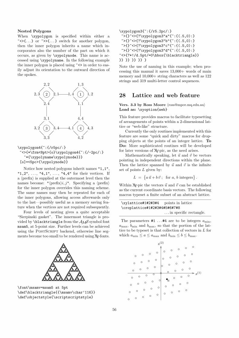
Nested PolygonsWhen \xypolygon is specified within either a~<>{. . . } or ~>>{. . . } switch for another polygon,then the inner polygon inherits a name which in-corporates also the number of the part on which itoccurs, as given by \xypolynode. This name is ac-cessed using \xypolyname. In the following examplethe inner polygon is placed using ~<> in order to eas-ily adjust its orientation to the outward direction ofthe spokes.
1?>=<89:;1, 1
1, 2����
1, 3????1, 4
����
????2?>=<89:; 2, 1
2, 2????2, 3
����
2, 4???? ����
3?>=<89:;3, 1
3, 2����
3, 3???? 3, 4
����
????4?>=<89:;4, 1
4, 2???? 4, 3
����
4, 4????����
\xypolygon4{~:{/r5pc/:}~<>{*\frm<8pt>{o}\xypolygon4{~:{/-2pc/:}
~*{\xypolyname\xypolynode}}}[o]=<5pc>{\xypolynode}}
Notice how nested polygons inherit names "1,1","1,2", . . . , "4,1", . . . , "4,4" for their vertices. Ifa 〈prefix〉 is supplied at the outermost level then thenames become: "〈prefix〉i, j". Specifying a 〈prefix〉for the inner polygon overrides this naming scheme.The same names may then be repeated for each ofthe inner polygons, allowing access afterwards onlyto the last—possibly useful as a memory saving fea-ture when the vertices are not required subsequently.
Four levels of nesting gives a quite acceptable“Sierpinski gasket”. The innermost triangle is pro-vided by \blacktriangle from theAMS symbol fontmsam5, at 5-point size. Further levels can be achievedusing the PostScript backend, otherwise line seg-ments become too small to be rendered usingXY-fonts.
NN N
11N
N N11 NN N
11N
N N11
NN N
11 NN N
11 NN N
11N
N N11 NN N
11N
N N11
NN N
11 NN N
11N
N N11
NN N
11 NN N
11 NN N
11N
N N11 NN N
11
NN N
11N
N N11 NN N
11N
N N11
NN N
11 NN N
11 NN N
11N
N N11 NN N
11N
N N11
NN N
11 NN N
11N
N N11
NN N
11 NN N
11 NN N
11N
N N11 NN N
11N
N N11
NN N
11 NN N
11N
N N11
NN N
11 NN N
11 NN N
11N
N N11 NN N
11
NN N
11N
N N11 NN N
11N
N N11
NN N
11 NN N
11 NN N
11N
N N11 NN N
11
NN N
11N
N N11 NN N
11N
N N11
NN N
11 NN N
11 NN N
11N
N N11 NN N
11N
N N11
NN N
11 NN N
11N
N N11
NN N
11 NN N
11 NN N
11N
N N11 NN N
11
NN N
11N
N N11 NN N
11N
N N11
NN N
11 NN N
11 NN N
11N
N N11 NN N
11
\font\msamv=msam5 at 5pt\def\blacktriangle{{\msamv\char’116}}\def\objectstyle{\scriptscriptstyle}
\xypolygon3{~:{/r5.2pc/:}~>{}~<>{?\xypolygon3"a"{~:{(.5,0):}~>{}~<>{?\xypolygon3"b"{~:{(.5,0):}~>{}~<>{?\xypolygon3"c"{~:{(.5,0):}~>{}~<>{?\xypolygon3"d"{~:{(.5,0):}
~<>{?*!/d.5pt/=0\hbox{\blacktriangle}}}} }} }} }} }
Note the use of naming in this example; when pro-cessing this manual it saves 13,000+ words of mainmemory and 10,000+ string characters as well as 122strings and 319 multi-letter control sequences.
28 Lattice and web feature
Vers. 3.3 by Ross Moore 〈[email protected]〉Load as: \xyoption{web}
This feature provides macros to facilitate typesettingof arrangements of points within a 2-dimensional lat-tice or “web-like” structure.
Currently the only routines implemented with thisfeature are some “quick and dirty” macros for drop-ping objects at the points of an integer lattice. ToDo: More sophisticated routines will be developedfor later versions of XY-pic, as the need arises.
Mathematically speaking, let ~u and ~v be vectorspointing in independent directions within the plane.Then the lattice spanned by ~u and ~v is the infiniteset of points L given by:
L ={a~u+ b~v ; for a, b integers
}.
Within XY-pic the vectors ~u and ~v can be establishedas the current coordinate basis vectors. The followingmacros typeset a finite subset of an abstract lattice.
\xylattice#1#2#3#4 points in lattice\croplattice#1#2#3#4#5#6#7#8
. . . in specific rectangle.
The parameters #1 . . . #4 are to be integers amin,amax, bmin and bmax, so that the portion of the lat-tice to be typeset is that collection of vectors in L forwhich amin ≤ a ≤ amax and bmin ≤ b ≤ bmax.
◦
◦
◦
◦
◦
◦
◦
◦
◦
◦
◦
◦
◦
◦
◦
◦
◦
◦
◦
◦
◦
◦
◦
◦
◦
◦
◦
◦
◦
◦
◦
◦
◦
◦
◦
◦
◦
◦
◦
◦
◦
◦
◦
◦
◦
◦
◦
◦
◦
◦
◦
◦
◦
◦
◦
◦
◦
◦
◦
◦
◦
◦
•as(1)//
s(2)OO
56
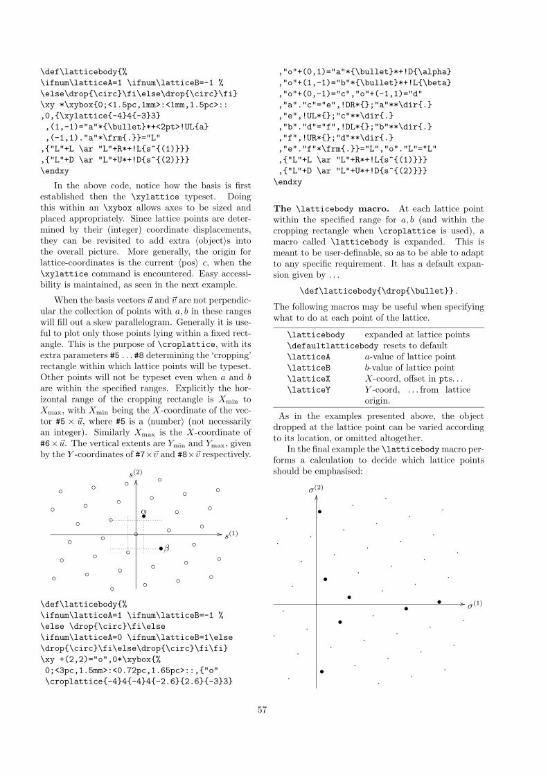
\def\latticebody{%\ifnum\latticeA=1 \ifnum\latticeB=-1 %\else\drop{\circ}\fi\else\drop{\circ}\fi}\xy *\xybox{0;<1.5pc,1mm>:<1mm,1.5pc>::,0,{\xylattice{-4}4{-3}3},(1,-1)="a"*{\bullet}*+<2pt>!UL{a},(-1,1)."a"*\frm{.}}="L"
,{"L"+L \ar "L"+R*+!L{s^{(1)}}},{"L"+D \ar "L"+U*+!D{s^{(2)}}}\endxy
In the above code, notice how the basis is firstestablished then the \xylattice typeset. Doingthis within an \xybox allows axes to be sized andplaced appropriately. Since lattice points are deter-mined by their (integer) coordinate displacements,they can be revisited to add extra 〈object〉s intothe overall picture. More generally, the origin forlattice-coordinates is the current 〈pos〉 c, when the\xylattice command is encountered. Easy accessi-bility is maintained, as seen in the next example.
When the basis vectors ~u and ~v are not perpendic-ular the collection of points with a, b in these rangeswill fill out a skew parallelogram. Generally it is use-ful to plot only those points lying within a fixed rect-angle. This is the purpose of \croplattice, with itsextra parameters #5 . . . #8 determining the ‘cropping’rectangle within which lattice points will be typeset.Other points will not be typeset even when a and bare within the specified ranges. Explicitly the hor-izontal range of the cropping rectangle is Xmin toXmax, with Xmin being the X-coordinate of the vec-tor #5 × ~u, where #5 is a 〈number〉 (not necessarilyan integer). Similarly Xmax is the X-coordinate of#6×~u. The vertical extents are Ymin and Ymax, givenby the Y -coordinates of #7×~v and #8×~v respectively.
◦
◦
◦
◦
◦
◦
◦
◦
◦
◦
◦
◦
◦
◦
◦
◦
◦
◦
◦
◦
◦
◦
◦
◦
◦
◦
◦
◦
◦
◦
◦
◦
◦
•α
•βs(1)//
s(2)OO
\def\latticebody{%\ifnum\latticeA=1 \ifnum\latticeB=-1 %\else \drop{\circ}\fi\else\ifnum\latticeA=0 \ifnum\latticeB=1\else\drop{\circ}\fi\else\drop{\circ}\fi\fi}\xy +(2,2)="o",0*\xybox{%0;<3pc,1.5mm>:<0.72pc,1.65pc>::,{"o"\croplattice{-4}4{-4}4{-2.6}{2.6}{-3}3}
,"o"+(0,1)="a"*{\bullet}*+!D{\alpha},"o"+(1,-1)="b"*{\bullet}*+!L{\beta},"o"+(0,-1)="c","o"+(-1,1)="d","a"."c"="e",!DR*{};"a"**\dir{.},"e",!UL*{};"c"**\dir{.},"b"."d"="f",!DL*{};"b"**\dir{.},"f",!UR*{};"d"**\dir{.},"e"."f"*\frm{.}}="L","o"."L"="L",{"L"+L \ar "L"+R*+!L{s^{(1)}}},{"L"+D \ar "L"+U*+!D{s^{(2)}}}
\endxy
The \latticebody macro. At each lattice pointwithin the specified range for a, b (and within thecropping rectangle when \croplattice is used), amacro called \latticebody is expanded. This ismeant to be user-definable, so as to be able to adaptto any specific requirement. It has a default expan-sion given by . . .
\def\latticebody{\drop{\bullet}} .
The following macros may be useful when specifyingwhat to do at each point of the lattice.
\latticebody expanded at lattice points\defaultlatticebody resets to default\latticeA a-value of lattice point\latticeB b-value of lattice point\latticeX X-coord, offset in pts. . .\latticeY Y -coord, . . . from lattice
origin.
As in the examples presented above, the objectdropped at the lattice point can be varied accordingto its location, or omitted altogether.
In the final example the \latticebody macro per-forms a calculation to decide which lattice pointsshould be emphasised:
.
.
.
.
.
.
.
•
.
.
.
.
•
.
.
.
•
.
•
•
.
.
.
.
.
.
.
.
.
.
.
.
.
.
•
.
.
.
.
.
.
.
•
.
.
.
.
.
σ(1)//
σ(2)OO
57
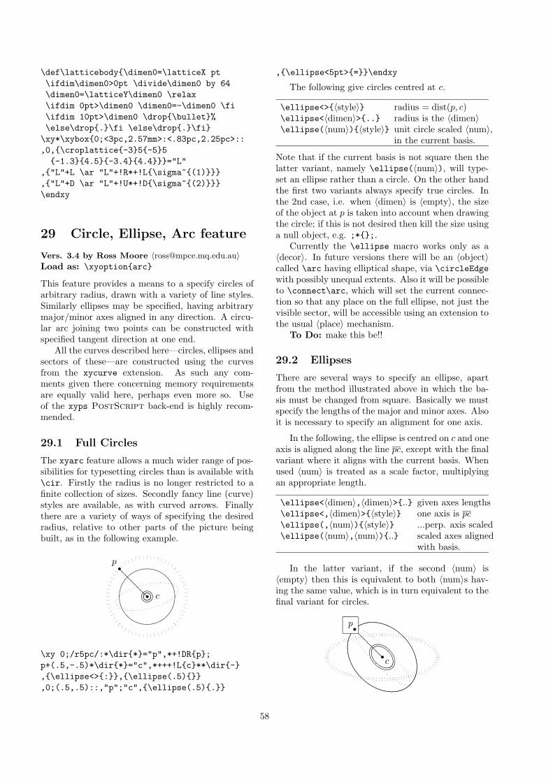
\def\latticebody{\dimen0=\latticeX pt\ifdim\dimen0>0pt \divide\dimen0 by 64\dimen0=\latticeY\dimen0 \relax\ifdim 0pt>\dimen0 \dimen0=-\dimen0 \fi\ifdim 10pt>\dimen0 \drop{\bullet}%\else\drop{.}\fi \else\drop{.}\fi}
\xy*\xybox{0;<3pc,2.57mm>:<.83pc,2.25pc>::,0,{\croplattice{-3}5{-5}5
{-1.3}{4.5}{-3.4}{4.4}}}="L",{"L"+L \ar "L"+!R*+!L{\sigma^{(1)}}},{"L"+D \ar "L"+!U*+!D{\sigma^{(2)}}}\endxy
29 Circle, Ellipse, Arc feature
Vers. 3.4 by Ross Moore 〈[email protected]〉Load as: \xyoption{arc}
This feature provides a means to a specify circles ofarbitrary radius, drawn with a variety of line styles.Similarly ellipses may be specified, having arbitrarymajor/minor axes aligned in any direction. A circu-lar arc joining two points can be constructed withspecified tangent direction at one end.
All the curves described here—circles, ellipses andsectors of these—are constructed using the curvesfrom the xycurve extension. As such any com-ments given there concerning memory requirementsare equally valid here, perhaps even more so. Useof the xyps PostScript back-end is highly recom-mended.
29.1 Full Circles
The xyarc feature allows a much wider range of pos-sibilities for typesetting circles than is available with\cir. Firstly the radius is no longer restricted to afinite collection of sizes. Secondly fancy line (curve)styles are available, as with curved arrows. Finallythere are a variety of ways of specifying the desiredradius, relative to other parts of the picture beingbuilt, as in the following example.
•p
• c?????????
\xy 0;/r5pc/:*\dir{*}="p",*+!DR{p};p+(.5,-.5)*\dir{*}="c",*+++!L{c}**\dir{-},{\ellipse<>{:}},{\ellipse(.5){}},0;(.5,.5)::,"p";"c",{\ellipse(.5){.}}
,{\ellipse<5pt>{=}}\endxy
The following give circles centred at c.
\ellipse<>{〈style〉} radius = dist(p, c)\ellipse<〈dimen〉>{..} radius is the 〈dimen〉\ellipse(〈num〉){〈style〉} unit circle scaled 〈num〉,
in the current basis.
Note that if the current basis is not square then thelatter variant, namely \ellipse(〈num〉), will type-set an ellipse rather than a circle. On the other handthe first two variants always specify true circles. Inthe 2nd case, i.e. when 〈dimen〉 is 〈empty〉, the sizeof the object at p is taken into account when drawingthe circle; if this is not desired then kill the size usinga null object, e.g. ;*{};.
Currently the \ellipse macro works only as a〈decor〉. In future versions there will be an 〈object〉called \arc having elliptical shape, via \circleEdgewith possibly unequal extents. Also it will be possibleto \connect\arc, which will set the current connec-tion so that any place on the full ellipse, not just thevisible sector, will be accessible using an extension tothe usual 〈place〉 mechanism.
To Do: make this be!!
29.2 Ellipses
There are several ways to specify an ellipse, apartfrom the method illustrated above in which the ba-sis must be changed from square. Basically we mustspecify the lengths of the major and minor axes. Alsoit is necessary to specify an alignment for one axis.
In the following, the ellipse is centred on c and oneaxis is aligned along the line pc, except with the finalvariant where it aligns with the current basis. Whenused 〈num〉 is treated as a scale factor, multiplyingan appropriate length.
\ellipse<〈dimen〉,〈dimen〉>{..} given axes lengths\ellipse<,〈dimen〉>{〈style〉} one axis is pc\ellipse(,〈num〉){〈style〉} ...perp. axis scaled\ellipse(〈num〉,〈num〉){..} scaled axes aligned
with basis.
In the latter variant, if the second 〈num〉 is〈empty〉 then this is equivalent to both 〈num〉s hav-ing the same value, which is in turn equivalent to thefinal variant for circles.
•p
•????????
c
58
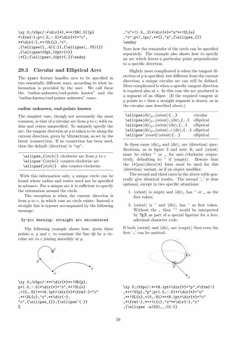
\xy 0;/r5pc/:*\dir{*},*++!DR(.5){p}*\frm{-};p+(.5,-.5)*\dir{*}="c",**\dir{-},*+!UL{c},"c",,{\ellipse(1,.4){:}},{\ellipse(,.75){}},{\ellipse<15pt,10pt>{=}};*{};{\ellipse<,10pt>{.}}\endxy
29.3 Circular and Elliptical Arcs
The xyarc feature handles arcs to be specified intwo essentially different ways, according to what in-formation is provided by the user. We call thesethe “radius-unknown/end-points known” and the“radius-known/end-points unknown” cases.
radius unknown, end-points known
The simplest case, though not necessarily the mostcommon, is that of a circular arc from p to c, with ra-dius and centre unspecified. To uniquely specify thearc, the tangent direction at p is taken to be along thecurrent direction, given by \Direction, as set by thelatest 〈connect〉ion. If no connection has been used,then the default 〈direction〉 is “up”.
\ellipse_{〈style〉} clockwise arc from p to c\ellipse^{〈style〉} counter-clockwise arc\ellipse{〈style〉} also counter-clockwise
With this information only, a unique circle can befound whose radius and centre need not be specifiedin advance. For a unique arc it is sufficient to specifythe orientation around the circle.
The exception is when the current direction isfrom p to c, in which case no circle exists. Instead astraight line is typeset accompanied by the followingmessage:
Xy-pic Warning: straight arc encountered
The following example shows how, given threepoints o, p and c, to continue the line op by a cir-cular arc to c joining smoothly at p.
•p
•o
•c
?????????
•a
\xy 0;/r5pc/:*=+\dir{*}*+!UR{p};p+(.5,-.5)*\dir{*}="o",*+!UL{o},+(0,.81)*=<6.1pt>\dir{*}*\frm{-}="c",*+!DL{c},"o",**\dir{-},"c",{\ellipse_{}},{\ellipse^{.}}%
,"o"+(1.5,.2)*\dir{*}="a"*+!UL{a},"o";p+/_1pc/,**{},"a",{\ellipse_{}}\endxy
Note how the remainder of the circle can be specifiedseparately. The example also shows how to specifyan arc which leaves a particular point perpendicularto a specific direction.
Slightly more complicated is when the tangent di-rection at p is specified, but different from the currentdirection; a unique circular arc can still be defined.More complicated is when a specific tangent directionis required also at c. In this case the arc produced isa segment of an ellipse. (If the required tangent atp points to c then a straight segment is drawn, as inthe circular case described above.)
\ellipse〈dir〉p,〈orient〉{..} circular\ellipse〈dir〉p,〈orient〉,〈dir〉c{..} elliptical\ellipse〈dir〉p,〈orient〉〈dir〉c{..} elliptical\ellipse〈dir〉p,〈orient〉,=〈dir〉c{..} elliptical\ellipse‘〈coord〉〈orient〉{..} elliptical
In these cases 〈dir〉p and 〈dir〉c are 〈direction〉 spec-ifications, as in figure 3 and note 4l, and 〈orient〉must be either ^ or _ for anti-/clockwise respec-tively, defaulting to ^ if 〈empty〉. Beware thatthe (*〈pos〉〈decor〉*) form must be used for this〈direction〉 variant, as if an object modifier.
The second and third cases in the above table gen-erally give identical results. The second ‘,’ is thusoptional, except in two specific situations:
1. 〈orient〉 is empty and 〈dir〉c has ^ or _ as thefirst token;
2. 〈orient〉 is ^ and 〈dir〉c has ^ as first token.Without the , then ^^ would be interpretedby TEX as part of a special ligature for a hex-adecimal character code.
If both 〈orient〉 and 〈dir〉c are 〈empty〉 then even thefirst ‘,’ can be omitted.
•p
•o
• c
?????????
\xy 0;/r5pc/:*=<8.1pt>\dir{*}="p",*\frm{-},*++!U{p},"p";p+(.5,-.5)*+\dir{*}="o",*+!UL{o},+(0,.81)*=<8.1pt>\dir{*}="c",*\frm{-},*++!L{c},"o"**\dir{-},"c",{\ellipse :a(50),_:0{:}}
59
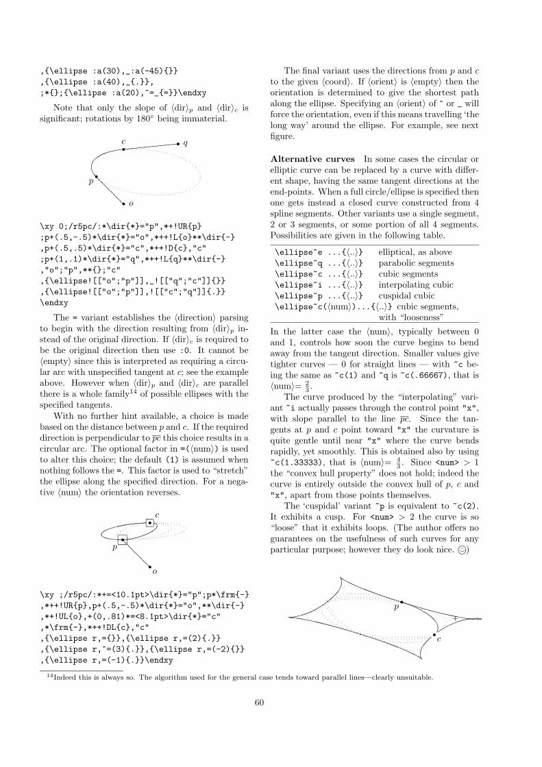
,{\ellipse :a(30),_:a(-45){}},{\ellipse :a(40),_{.}},;*{};{\ellipse :a(20),^=_{=}}\endxy
Note that only the slope of 〈dir〉p and 〈dir〉c issignificant; rotations by 180◦ being immaterial.
•p
• o?????????
•c • qbbbbbbbbbbbbb
\xy 0;/r5pc/:*\dir{*}="p",*+!UR{p};p+(.5,-.5)*\dir{*}="o",*++!L{o}**\dir{-},p+(.5,.5)*\dir{*}="c",*++!D{c},"c";p+(1,.1)*\dir{*}="q",*++!L{q}**\dir{-},"o";"p",**{};"c",{\ellipse![["o";"p"]],_![["q";"c"]]{}},{\ellipse![["o";"p"]],![["c";"q"]]{.}}\endxy
The = variant establishes the 〈direction〉 parsingto begin with the direction resulting from 〈dir〉p in-stead of the original direction. If 〈dir〉c is required tobe the original direction then use :0. It cannot be〈empty〉 since this is interpreted as requiring a circu-lar arc with unspecified tangent at c; see the exampleabove. However when 〈dir〉p and 〈dir〉c are parallelthere is a whole family14 of possible ellipses with thespecified tangents.
With no further hint available, a choice is madebased on the distance between p and c. If the requireddirection is perpendicular to pc this choice results in acircular arc. The optional factor in =(〈num〉) is usedto alter this choice; the default (1) is assumed whennothing follows the =. This factor is used to “stretch”the ellipse along the specified direction. For a nega-tive 〈num〉 the orientation reverses.
•p
•?????????
o
•c
\xy ;/r5pc/:*+=<10.1pt>\dir{*}="p";p*\frm{-},*++!UR{p},p+(.5,-.5)*\dir{*}="o",**\dir{-},*+!UL{o},+(0,.81)*=<8.1pt>\dir{*}="c",*\frm{-},*++!DL{c},"c",{\ellipse r,={}},{\ellipse r,=(2){.}},{\ellipse r,^=(3){.}},{\ellipse r,=(-2){}},{\ellipse r,=(-1){.}}\endxy
The final variant uses the directions from p and cto the given 〈coord〉. If 〈orient〉 is 〈empty〉 then theorientation is determined to give the shortest pathalong the ellipse. Specifying an 〈orient〉 of ^ or _ willforce the orientation, even if this means travelling ‘thelong way’ around the ellipse. For example, see nextfigure.
Alternative curves In some cases the circular orelliptic curve can be replaced by a curve with differ-ent shape, having the same tangent directions at theend-points. When a full circle/ellipse is specified thenone gets instead a closed curve constructed from 4spline segments. Other variants use a single segment,2 or 3 segments, or some portion of all 4 segments.Possibilities are given in the following table.
\ellipse~e ...{〈..〉} elliptical, as above\ellipse~q ...{〈..〉} parabolic segments\ellipse~c ...{〈..〉} cubic segments\ellipse~i ...{〈..〉} interpolating cubic\ellipse~p ...{〈..〉} cuspidal cubic\ellipse~c(〈num〉)...{〈..〉} cubic segments,
with “looseness”
In the latter case the 〈num〉, typically between 0and 1, controls how soon the curve begins to bendaway from the tangent direction. Smaller values givetighter curves — 0 for straight lines — with ~c be-ing the same as ~c(1) and ~q is ~c(.66667), that is〈num〉= 2
3 .The curve produced by the “interpolating” vari-
ant ~i actually passes through the control point "x",with slope parallel to the line pc. Since the tan-gents at p and c point toward "x" the curvature isquite gentle until near "x" where the curve bendsrapidly, yet smoothly. This is obtained also by using~c(1.33333), that is 〈num〉= 4
3 . Since <num> > 1the “convex hull property” does not hold; indeed thecurve is entirely outside the convex hull of p, c and"x", apart from those points themselves.
The ‘cuspidal’ variant ~p is equivalent to ~c(2).It exhibits a cusp. For <num> > 2 the curve is so“loose” that it exhibits loops. (The author offers noguarantees on the usefulness of such curves for anyparticular purpose; however they do look nice. ©)
•p
•c
_�
14Indeed this is always so. The algorithm used for the general case tends toward parallel lines—clearly unsuitable.
60
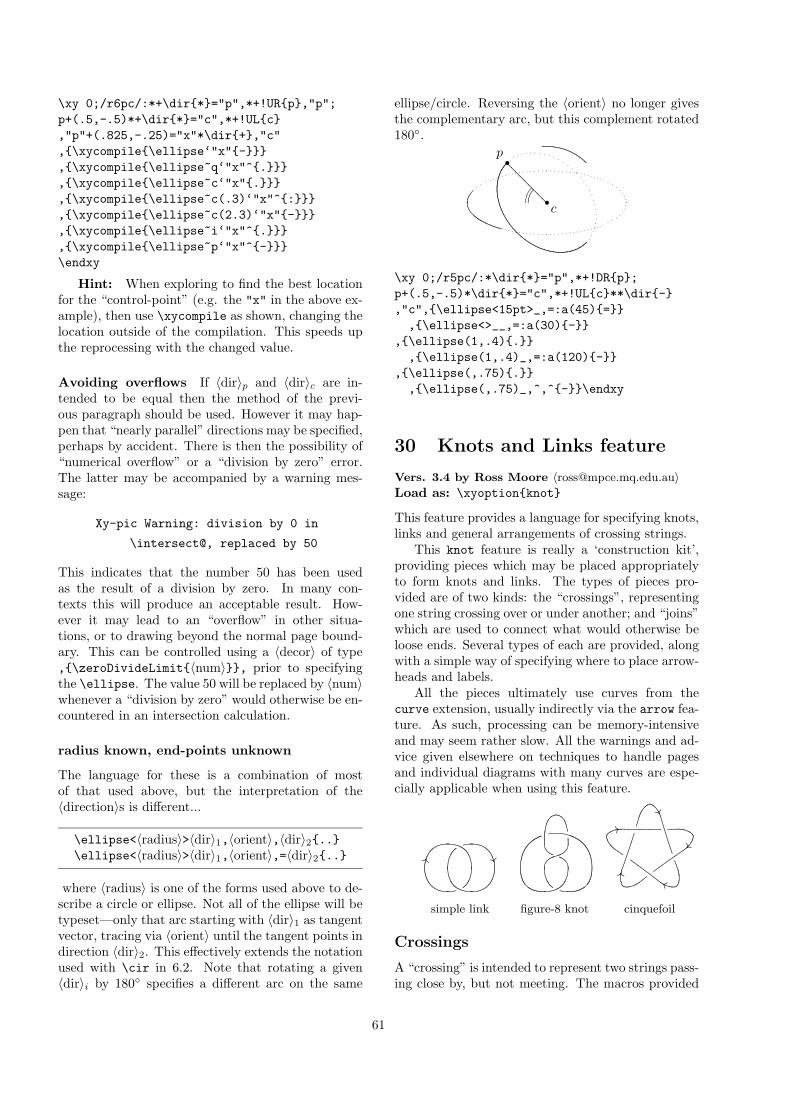
\xy 0;/r6pc/:*+\dir{*}="p",*+!UR{p},"p";p+(.5,-.5)*+\dir{*}="c",*+!UL{c},"p"+(.825,-.25)="x"*\dir{+},"c",{\xycompile{\ellipse‘"x"{-}}},{\xycompile{\ellipse~q‘"x"^{.}}},{\xycompile{\ellipse~c‘"x"{.}}},{\xycompile{\ellipse~c(.3)‘"x"^{:}}},{\xycompile{\ellipse~c(2.3)‘"x"{-}}},{\xycompile{\ellipse~i‘"x"^{.}}},{\xycompile{\ellipse~p‘"x"^{-}}}\endxy
Hint: When exploring to find the best locationfor the “control-point” (e.g. the "x" in the above ex-ample), then use \xycompile as shown, changing thelocation outside of the compilation. This speeds upthe reprocessing with the changed value.
Avoiding overflows If 〈dir〉p and 〈dir〉c are in-tended to be equal then the method of the previ-ous paragraph should be used. However it may hap-pen that “nearly parallel” directions may be specified,perhaps by accident. There is then the possibility of“numerical overflow” or a “division by zero” error.The latter may be accompanied by a warning mes-sage:
Xy-pic Warning: division by 0 in
\intersect@, replaced by 50
This indicates that the number 50 has been usedas the result of a division by zero. In many con-texts this will produce an acceptable result. How-ever it may lead to an “overflow” in other situa-tions, or to drawing beyond the normal page bound-ary. This can be controlled using a 〈decor〉 of type,{\zeroDivideLimit{〈num〉}}, prior to specifyingthe \ellipse. The value 50 will be replaced by 〈num〉whenever a “division by zero” would otherwise be en-countered in an intersection calculation.
radius known, end-points unknown
The language for these is a combination of mostof that used above, but the interpretation of the〈direction〉s is different...
\ellipse<〈radius〉>〈dir〉1,〈orient〉,〈dir〉2{..}\ellipse<〈radius〉>〈dir〉1,〈orient〉,=〈dir〉2{..}
where 〈radius〉 is one of the forms used above to de-scribe a circle or ellipse. Not all of the ellipse will betypeset—only that arc starting with 〈dir〉1 as tangentvector, tracing via 〈orient〉 until the tangent points indirection 〈dir〉2. This effectively extends the notationused with \cir in 6.2. Note that rotating a given〈dir〉i by 180◦ specifies a different arc on the same
ellipse/circle. Reversing the 〈orient〉 no longer givesthe complementary arc, but this complement rotated180◦.
•p
•c
?????????
\xy 0;/r5pc/:*\dir{*}="p",*+!DR{p};p+(.5,-.5)*\dir{*}="c",*+!UL{c}**\dir{-},"c",{\ellipse<15pt>_,=:a(45){=}}
,{\ellipse<>__,=:a(30){-}},{\ellipse(1,.4){.}}
,{\ellipse(1,.4)_,=:a(120){-}},{\ellipse(,.75){.}}
,{\ellipse(,.75)_,^,^{-}}\endxy
30 Knots and Links feature
Vers. 3.4 by Ross Moore 〈[email protected]〉Load as: \xyoption{knot}
This feature provides a language for specifying knots,links and general arrangements of crossing strings.
This knot feature is really a ‘construction kit’,providing pieces which may be placed appropriatelyto form knots and links. The types of pieces pro-vided are of two kinds: the “crossings”, representingone string crossing over or under another; and “joins”which are used to connect what would otherwise beloose ends. Several types of each are provided, alongwith a simple way of specifying where to place arrow-heads and labels.
All the pieces ultimately use curves from thecurve extension, usually indirectly via the arrow fea-ture. As such, processing can be memory-intensiveand may seem rather slow. All the warnings and ad-vice given elsewhere on techniques to handle pagesand individual diagrams with many curves are espe-cially applicable when using this feature.
JJ ��
simple link figure-8 knot
��
��
22
MMgg
cinquefoil
Crossings
A “crossing” is intended to represent two strings pass-ing close by, but not meeting. The macros provided
61
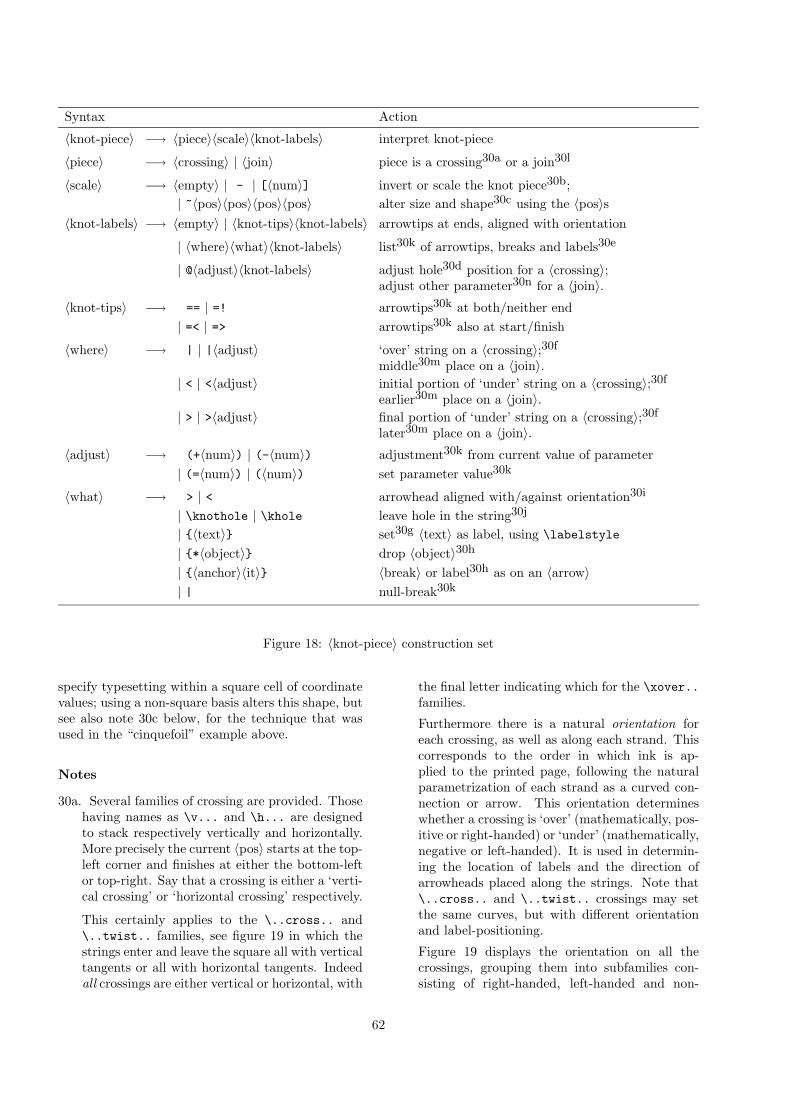
Syntax Action
〈knot-piece〉 −→ 〈piece〉〈scale〉〈knot-labels〉 interpret knot-piece
〈piece〉 −→ 〈crossing〉 | 〈join〉 piece is a crossing30a or a join30l
〈scale〉 −→ 〈empty〉 | - | [〈num〉] invert or scale the knot piece30b;| ~〈pos〉〈pos〉〈pos〉〈pos〉 alter size and shape30c using the 〈pos〉s
〈knot-labels〉 −→ 〈empty〉 | 〈knot-tips〉〈knot-labels〉 arrowtips at ends, aligned with orientation
| 〈where〉〈what〉〈knot-labels〉 list30k of arrowtips, breaks and labels30e
| @〈adjust〉〈knot-labels〉 adjust hole30d position for a 〈crossing〉;adjust other parameter30n for a 〈join〉.
〈knot-tips〉 −→ == | =! arrowtips30k at both/neither end| =< | => arrowtips30k also at start/finish
〈where〉 −→ | | |〈adjust〉 ‘over’ string on a 〈crossing〉;30f
middle30m place on a 〈join〉.| < | <〈adjust〉 initial portion of ‘under’ string on a 〈crossing〉;30f
earlier30m place on a 〈join〉.| > | >〈adjust〉 final portion of ‘under’ string on a 〈crossing〉;30f
later30m place on a 〈join〉.〈adjust〉 −→ (+〈num〉) | (-〈num〉) adjustment30k from current value of parameter
| (=〈num〉) | (〈num〉) set parameter value30k
〈what〉 −→ > | < arrowhead aligned with/against orientation30i
| \knothole | \khole leave hole in the string30j
| {〈text〉} set30g 〈text〉 as label, using \labelstyle
| {*〈object〉} drop 〈object〉30h
| {〈anchor〉〈it〉} 〈break〉 or label30h as on an 〈arrow〉| | null-break30k
Figure 18: 〈knot-piece〉 construction set
specify typesetting within a square cell of coordinatevalues; using a non-square basis alters this shape, butsee also note 30c below, for the technique that wasused in the “cinquefoil” example above.
Notes
30a. Several families of crossing are provided. Thosehaving names as \v... and \h... are designedto stack respectively vertically and horizontally.More precisely the current 〈pos〉 starts at the top-left corner and finishes at either the bottom-leftor top-right. Say that a crossing is either a ‘verti-cal crossing’ or ‘horizontal crossing’ respectively.
This certainly applies to the \..cross.. and\..twist.. families, see figure 19 in which thestrings enter and leave the square all with verticaltangents or all with horizontal tangents. Indeedall crossings are either vertical or horizontal, with
the final letter indicating which for the \xover..families.
Furthermore there is a natural orientation foreach crossing, as well as along each strand. Thiscorresponds to the order in which ink is ap-plied to the printed page, following the naturalparametrization of each strand as a curved con-nection or arrow. This orientation determineswhether a crossing is ‘over’ (mathematically, pos-itive or right-handed) or ‘under’ (mathematically,negative or left-handed). It is used in determin-ing the location of labels and the direction ofarrowheads placed along the strings. Note that\..cross.. and \..twist.. crossings may setthe same curves, but with different orientationand label-positioning.
Figure 19 displays the orientation on all thecrossings, grouping them into subfamilies con-sisting of right-handed, left-handed and non-
62
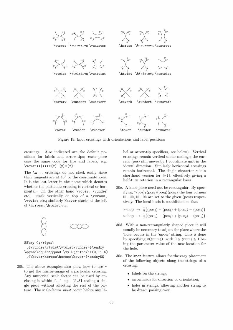
��yFFx
FFz ��x
��z
FFy EEy
EEx �� z
77y
ffx
ffz
77x
77z
ffy
eey
eex
::z
\vcross \vcrossneg \vuncross \hcross \hcrossneg \huncross
��y
�� x
�� z
��x
��z �� y ��y
�� x
��z ((
y77x
77z ((x
((z
77y
::y
::x $$z
\vtwist \vtwistneg \vuntwist \htwist \htwistneg \huntwist
��y
��x
��z
��x
��z
��y
�� y�� x
�� z
��y
??x
??z
��x
��z
??y
99y
99x %%z
\xoverv \xunderv \xunoverv \xoverh \xunderh \xunoverh
�� yJJx
11z --x
�� zJJy
33y
KKx �� z
44y
jjx
QQz
MMx
44z
jjy
SSy
kkx
33z
\vover \vunder \vunover \hover \hunder \hunover
Figure 19: knot crossings with orientations and label positions
crossings. Also indicated are the default po-sitions for labels and arrow-tips; each pieceuses the same code for tips and labels, e.g.\vover<>|>>><{x}|{y}>{z}.
The \x... crossings do not stack easily sincetheir tangents are at 45◦ to the coordinate axes.It is the last letter in the name which denoteswhether the particular crossing is vertical or hor-izontal. On the other hand \vover , \vunderetc. stack vertically on top of a \vcross ,\vtwist etc.; similarly \hover stacks at the leftof \hcross , \htwist etc.
$$\xy 0;/r1pc/:,{\vunder\vtwist\vtwist\vunder-}\endxy
\qquad\qquad\qquad \xy 0;/r1pc/:+(0,-1.5),{\hover\hcross\hcross\hover-}\endxy$$
30b. The above examples also show how to use -to get the mirror-image of a particular crossing.Any numerical scale factor can be used by en-closing it within [..] e.g. [2.3] scaling a sin-gle piece without affecting the rest of the pic-ture. The scale-factor must occur before any la-
bel or arrow-tip specifiers, see below). Verticalcrossings remain vertical under scalings; the cur-rent 〈pos〉 still moves by 1 coordinate unit in the‘down’ direction. Similarly horizontal crossingsremain horizontal. The single character - is ashorthand version for [-1], effectively giving ahalf-turn rotation in a rectangular basis.
30c. A knot-piece need not be rectangular. By spec-ifying ~〈pos〉1〈pos2〉〈pos3〉〈pos4〉 the four cornersUL, UR, DL, DR are set to the given 〈pos〉s respec-tively. The local basis is established so that
r–hop ↔ 12
(〈pos2〉 − 〈pos1〉+ 〈pos4〉 − 〈pos3〉
)u–hop ↔ 1
2
(〈pos1〉 − 〈pos3〉+ 〈pos2〉 − 〈pos1〉
).
30d. With a non-rectangularly shaped piece it willusually be necessary to adjust the place where the‘hole’ occurs in the ‘under’ string. This is doneby specifying @(〈num〉), with 0 ≤ 〈num〉 ≤ 1 be-ing the parameter value of the new location forthe hole.
30e. The knot feature allows for the easy placementof the following objects along the strings of acrossing:
• labels on the strings;• arrowheads for direction or orientation;• holes in strings, allowing another string to
be drawn passing over.
63
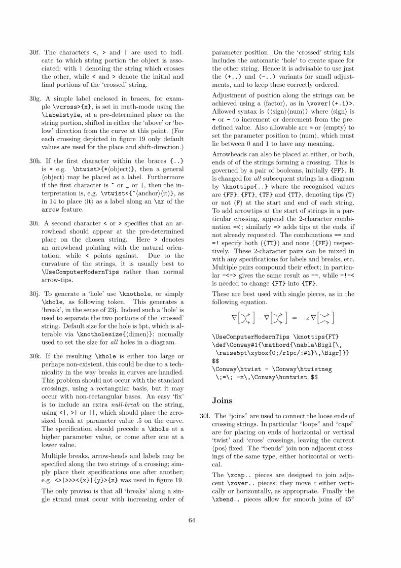
30f. The characters <, > and | are used to indi-cate to which string portion the object is asso-ciated; with | denoting the string which crossesthe other, while < and > denote the initial andfinal portions of the ‘crossed’ string.
30g. A simple label enclosed in braces, for exam-ple \vcross>{x}, is set in math-mode using the\labelstyle, at a pre-determined place on thestring portion, shifted in either the ‘above’ or ‘be-low’ direction from the curve at this point. (Foreach crossing depicted in figure 19 only defaultvalues are used for the place and shift-direction.)
30h. If the first character within the braces {..}is * e.g. \htwist>{*〈object〉}, then a general〈object〉 may be placed as a label. Furthermoreif the first character is ^ or _ or |, then the in-terpretation is, e.g. \vtwist<{^〈anchor〉〈it〉}, asin 14 to place 〈it〉 as a label along an \ar of thearrow feature.
30i. A second character < or > specifies that an ar-rowhead should appear at the pre-determinedplace on the chosen string. Here > denotesan arrowhead pointing with the natural orien-tation, while < points against. Due to thecurvature of the strings, it is usually best to\UseComputerModernTips rather than normalarrow-tips.
30j. To generate a ‘hole’ use \knothole, or simply\khole, as following token. This generates a‘break’, in the sense of 23j. Indeed such a ‘hole’ isused to separate the two portions of the ‘crossed’string. Default size for the hole is 5pt, which is al-terable via \knotholesize{〈dimen〉}; normallyused to set the size for all holes in a diagram.
30k. If the resulting \khole is either too large orperhaps non-existent, this could be due to a tech-nicality in the way breaks in curves are handled.This problem should not occur with the standardcrossings, using a rectangular basis, but it mayoccur with non-rectangular bases. An easy ‘fix’is to include an extra null-break on the string,using <|, >| or ||, which should place the zero-sized break at parameter value .5 on the curve.The specification should precede a \khole at ahigher parameter value, or come after one at alower value.
Multiple breaks, arrow-heads and labels may bespecified along the two strings of a crossing; sim-ply place their specifications one after another;e.g. <>|>>><{x}|{y}>{z} was used in figure 19.
The only proviso is that all ‘breaks’ along a sin-gle strand must occur with increasing order of
parameter position. On the ‘crossed’ string thisincludes the automatic ‘hole’ to create space forthe other string. Hence it is advisable to use justthe (+..) and (-..) variants for small adjust-ments, and to keep these correctly ordered.
Adjustment of position along the strings can beachieved using a 〈factor〉, as in \vover|(+.1)>.Allowed syntax is (〈sign〉〈num〉) where 〈sign〉 is+ or - to increment or decrement from the pre-defined value. Also allowable are = or 〈empty〉 toset the parameter position to 〈num〉, which mustlie between 0 and 1 to have any meaning.
Arrowheads can also be placed at either, or both,ends of of the strings forming a crossing. This isgoverned by a pair of booleans, initially {FF}. Itis changed for all subsequent strings in a diagramby \knottips{..} where the recognised valuesare {FF}, {FT}, {TF} and {TT}, denoting tips (T)or not (F) at the start and end of each string.To add arrowtips at the start of strings in a par-ticular crossing, append the 2-character combi-nation =< ; similarly => adds tips at the ends, ifnot already requested. The combinations == and=! specify both ({TT}) and none ({FF}) respec-tively. These 2-character pairs can be mixed inwith any specifications for labels and breaks, etc.Multiple pairs compound their effect; in particu-lar =<=> gives the same result as ==, while =!=<is needed to change {FT} into {TF}.
These are best used with single pieces, as in thefollowing equation.
∇[
//
//]−∇
[//
//]
= −z∇[
//
//
]\UseComputerModernTips \knottips{FT}\def\Conway#1{\mathord{\nabla\Bigl[\,\raise5pt\xybox{0;/r1pc/:#1}\,\Bigr]}}
$$\Conway\htwist - \Conway\htwistneg\;=\; -z\,\Conway\huntwist $$
Joins
30l. The “joins” are used to connect the loose ends ofcrossing strings. In particular “loops” and “caps”are for placing on ends of horizontal or vertical‘twist’ and ‘cross’ crossings, leaving the current〈pos〉 fixed. The “bends” join non-adjacent cross-ings of the same type, either horizontal or verti-cal.
The \xcap.. pieces are designed to join adja-cent \xover.. pieces; they move c either verti-cally or horizontally, as appropriate. Finally the\xbend.. pieces allow for smooth joins of 45◦
64
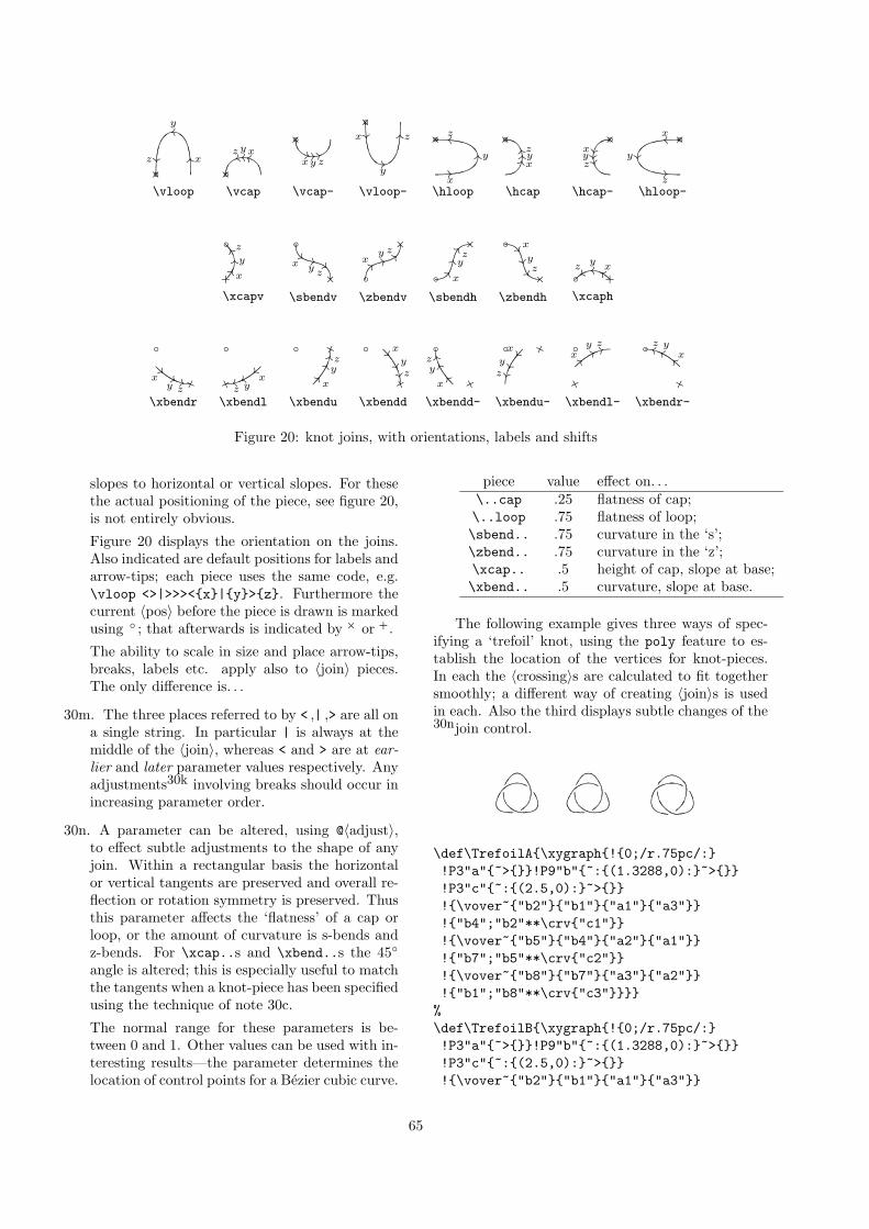
◦
PP x
ooy
��z?� ◦
jjxooy
ttz
?�
◦**x
//y
44z
?�◦��x
//y
NN z
?�◦
00x
OO y
nnz�? ◦
JJxOO yTT z
�? ◦x��y��z
�? ◦ppx
��y
..z
�?
\vloop \vcap \vcap- \vloop- \hloop \hcap \hcap- \hloop-
◦
EEx
OO y
YY z
_�
◦##
x ++y ##z �? ◦
;;x 33y ;;z
?�
◦CCx
KK y
CCz
?� ◦ �� x
�� y
�� z�? ◦ee xoo
yyyz �_
\xcapv \sbendv \zbendv \sbendh \zbendh \xcaph
◦
!!x ''y
++z �O
◦
}}xww
yssz
/o
◦
AAx
GGy
KKz
O� ◦ �� x
�� y�� z
o/
\xbendr \xbendl \xbendu \xbendd
◦
]]x
WWy
SSz
o/
◦ ��x
��y��z
O� ◦==x 77y 33z
/o
◦aa x
ggykkz
�O
\xbendd- \xbendu- \xbendl- \xbendr-
Figure 20: knot joins, with orientations, labels and shifts
slopes to horizontal or vertical slopes. For thesethe actual positioning of the piece, see figure 20,is not entirely obvious.
Figure 20 displays the orientation on the joins.Also indicated are default positions for labels andarrow-tips; each piece uses the same code, e.g.\vloop <>|>>><{x}|{y}>{z}. Furthermore thecurrent 〈pos〉 before the piece is drawn is markedusing ◦ ; that afterwards is indicated by �? or _�
.
The ability to scale in size and place arrow-tips,breaks, labels etc. apply also to 〈join〉 pieces.The only difference is. . .
30m. The three places referred to by < ,| ,> are all ona single string. In particular | is always at themiddle of the 〈join〉, whereas < and > are at ear-lier and later parameter values respectively. Anyadjustments30k involving breaks should occur inincreasing parameter order.
30n. A parameter can be altered, using @〈adjust〉,to effect subtle adjustments to the shape of anyjoin. Within a rectangular basis the horizontalor vertical tangents are preserved and overall re-flection or rotation symmetry is preserved. Thusthis parameter affects the ‘flatness’ of a cap orloop, or the amount of curvature is s-bends andz-bends. For \xcap..s and \xbend..s the 45◦
angle is altered; this is especially useful to matchthe tangents when a knot-piece has been specifiedusing the technique of note 30c.
The normal range for these parameters is be-tween 0 and 1. Other values can be used with in-teresting results—the parameter determines thelocation of control points for a Bezier cubic curve.
piece value effect on. . .\..cap .25 flatness of cap;\..loop .75 flatness of loop;\sbend.. .75 curvature in the ‘s’;\zbend.. .75 curvature in the ‘z’;\xcap.. .5 height of cap, slope at base;\xbend.. .5 curvature, slope at base.
The following example gives three ways of spec-ifying a ‘trefoil’ knot, using the poly feature to es-tablish the location of the vertices for knot-pieces.In each the 〈crossing〉s are calculated to fit togethersmoothly; a different way of creating 〈join〉s is usedin each. Also the third displays subtle changes of the30njoin control.
\def\TrefoilA{\xygraph{!{0;/r.75pc/:}!P3"a"{~>{}}!P9"b"{~:{(1.3288,0):}~>{}}!P3"c"{~:{(2.5,0):}~>{}}!{\vover~{"b2"}{"b1"}{"a1"}{"a3"}}!{"b4";"b2"**\crv{"c1"}}!{\vover~{"b5"}{"b4"}{"a2"}{"a1"}}!{"b7";"b5"**\crv{"c2"}}!{\vover~{"b8"}{"b7"}{"a3"}{"a2"}}!{"b1";"b8"**\crv{"c3"}}}}
%\def\TrefoilB{\xygraph{!{0;/r.75pc/:}!P3"a"{~>{}}!P9"b"{~:{(1.3288,0):}~>{}}!P3"c"{~:{(2.5,0):}~>{}}!{\vover~{"b2"}{"b1"}{"a1"}{"a3"}}
65
!{\vcap~{"c1"}{"c1"}{"b4"}{"b2"}@(+.1)}!{\vover~{"b5"}{"b4"}{"a2"}{"a1"}}!{\vcap~{"c2"}{"c2"}{"b7"}{"b5"}@(+.2)}!{\vover~{"b8"}{"b7"}{"a3"}{"a2"}}!{\vcap~{"c3"}{"c3"}{"b1"}{"b8"}}}}
%\def\TrefoilC{\xygraph{!{0;/r.75pc/:}!P3"a"{~>{}}!P12"b"{~:{(1.414,0):}~>{}}!{\vover~{"b2"}{"b1"}{"a1"}{"a3"}}!{\save 0;"b2"-"b5":"b5",
\xcaph @(+.1)\restore}!{\vover~{"b6"}{"b5"}{"a2"}{"a1"}}!{\save 0;"b6"-"b9":"b9",
\xcaph @(+.2)\restore}!{\vover~{"b10"}{"b9"}{"a3"}{"a2"}}!{\save 0;"b10"-"b1":"b1",
\xcaph @(+.3)\restore} }}$$\TrefoilA\quad\TrefoilB
\quad\TrefoilC$$
Changing the string-style
It is not necessary to use solid curves; any style avail-able to curves and arrows can be chosen using. . .
\knotstyle{〈char〉} use \dir{〈char〉}\knotstyles{〈char〉}{〈char〉} two styles\knotSTYLE{〈code〉} use 〈code〉
In each case the new style applies to all subse-quent knot pieces, except that the two styles applyonly to crossings. The latter case allows use of ob-ject 〈modifier〉s. The 〈code〉 consists of two groups{..}{..} , each containing 〈arrow〉 forms, as in 14and notes 23m, 23r. Only the first 〈arrow〉 form isused with 〈join〉s whereas the two forms are used re-spectively with the two strings of a 〈crossing〉 in theorder that they are drawn.
31 Smart Path option
Vers. 0.0 by George C. Necula 〈[email protected]〉Load as: \xyoption{smartpath}
This extends the ‘arrow’ feature, which is there-fore required, with a “smart” 〈path〉 between two〈pos〉itions.
The 〈turn〉 syntax is extended with the construc-tion
〈turn〉 −→‘s 〈diag〉 _ 〈diag〉 〈turnradius〉
\arin_out/5pt which draws a connector leaving p inthe in 〈diag〉onal direction and arrives at c in the out
〈diag〉onal direction, using 5pt turns. The connec-tor contains only horizontal or vertical lines and 1
8sectors of circles of the given (optional) 〈turnradius〉.
Bug: Any labels are placed at the end of the con-nection.
Bug: This code should probably be merged withthe ‘arrow’ feature.
Part IV
DriversThis part describes ‘drivers’ that customise the partsof the DVI file generated from XY-pictures to exploitspecial capabilities of particular DVI driver programsthrough TEXs \special command. This makes theDVI files non-portable but is needed for full supportof some of the XY-pic extensions (described in part II).
Figure 21 at the end of this part summarises theextensions supported by all drivers.
32 Support for Specific Drivers
32.1 dvidrv driver
Vers. 3.3 by Ross Moore 〈[email protected]〉Load as: \xyoption{dvidrv}
This driver provides support for the “emtex”\special commands, when using one of the stan-dard dvi-drivers: dvidot, dvihplj, dvimsp, dviscror dvivik, that come with Eberhard Mattes’ em-TEXdistribution.
Supported \special effects are...• em-TEX line-drawing \specials.• variable line-widths
32.2 DVIPS driver
Vers. 3.3 by Ross Moore 〈[email protected]〉Load as: \xyoption{dvips}
This driver provides support for all extensions whenusing the dvips driver by Tomas Rokicki [11]. It hasbeen tested with dvips version 5.55a and dvipsk ver-sion 5.58f.
Supported \special effects are...• colour, using direct color specials and PostScript.• crayon colours.• PostScript back-end.• rotated/scaled diagrams and text, using Post-
Script.• variable line-widths and poly-lines, using Post-
Script.
66
• extra frames and fills, using PostScript.
• patterns and tiles, using PostScript.
• tpic drawing commands.
• em-TEX drawing commands.
32.3 DVITOPS driver
Vers. 3.3 by Ross Moore 〈[email protected]〉Load as: \xyoption{dvitops}
This file provides support for the dvitops driver byJames Clark. As of September 1995, it has not beenfully tested.
Supported \special effects are...
• colour, using direct color specials for gray, rgb andhsb colour models; and PostScript colour withindiagrams;
• crayon colours.
• PostScript back-end.
• rotated/scaled diagrams and text, using dvitops
specials; however these may not be nested.
• variable line-widths and poly-lines, using Post-
Script.
• extra frames and fills, using PostScript.
• patterns and tiles, using PostScript
• tpic drawing commands.
32.4 OzTeX driver
Vers. 3.3 by Ross Moore 〈[email protected]〉Load as: \xyoption{oztex}
This driver provides the necessary interface to sup-port the PostScript back-end and other Post-
Script effects when using the DVI driver of versions1.8+ of OzTEX by Andrew Trevorrow,15 Earlier ver-sions of OzTEX should instead use the driver option\xyoption{17oztex}.
Effects such as colour, line-thickness and rotatedor scaled diagrams are only partially supported inthat the effects cannot be applied to any text or sym-bols placed using fonts. This is due to the natureof OzTEX 〈driver〉, whose optimization of the place-ment of font-characters precludes the applicability ofsuch effects. Furthermore the PostScript dictionarymust be available in a file called global.ps or ap-pended to the OzTeXdict.pro. However with ver-sion 1.8 and later of OzTEX, there is the alternative
of using the dvips 〈driver〉, which does support allthe PostScript effects available in XY-pic.
Note: To use XY-pic effectively with OzTEX re-quires changing several memory parameters. In par-ticular a ‘Big-TEX’ is needed, along with an increasein the pool_size parameter. Explicit instructionsare contained in the file INSTALL.OzTeX of the XY-picdistribution.
Supported \special effects are...
• colour, using PostScript, but not of font-characters.
• crayon colours, similarly restricted.
• PostScript back-end.
• variable line-widths and poly-lines, using Post-
Script.
• extra frames and fills, using PostScript.
• patterns and tiles, using PostScript.
• rotated/scaled diagrams and text, recognised butnot supported.
32.5 OzTeX v1.7 driver
Vers. 3.3 by Ross Moore 〈[email protected]〉Load as: \xyoption{17oztex}
This option provides the necessary interface to sup-port the PostScript back-end and other Post-
Script effects when using the DVI driver of ver-sion 1.7 of OzTEX by Andrew Trevorrow,16 Laterversions of OzTEX should instead use the driver op-tion \xyoption{oztex}. Upgrading to version 1.9+ofOzTEX is recommended.
Does not support rotations, scaling and colouredtext within diagrams and the PostScript dictionarymust be available in a file called global.ps.
Note: To use XY-pic effectively with OzTEX re-quires changing several memory parameters. In par-ticular a ‘Big-TEX’ is needed, along with an increasein the pool_size parameter. Explicit instructionsare contained in the file INSTALL.OzTeX of the XY-picdistribution.
Supported \special effects are...
• colour, using PostScript, but not of font-characters.
• crayon colours, similarly restricted.
• PostScript back-end.
• variable line-widths and poly-lines, using Post-
Script.
• extra frames and fills, using PostScript.15OzTEX is a shareware implementation of TEX for Macintosh available from many bulletin boards and ftp sites; v1.5 and earlier
versions were freeware. Email contact: 〈[email protected]〉.16OzTEX is a shareware implementation of TEX for Macintosh available from many bulletin boards and ftp sites; v1.5 and earlier
versions were freeware. Email contact: 〈[email protected]〉.
67
• patterns and tiles, using PostScript.
• rotated/scaled diagrams and text, recognised butnot supported.
32.6 Textures driver
Vers. 3.3 by Ross Moore 〈[email protected]〉Load as: \xyoption{textures}
This driver provides support for version 1.7+ ofBlue Sky Research’s Textures application for Mac-intosh17. It incorporates support for colour andall of XY-pic’s PostScript effects. Earlier versionsof Textures should instead use the driver option\xyoption{16textures}.
Notice that version 1.7 suffers from a printing bugwhich may cause a PostScript error. A fix is kludgedby making sure the first page has been shown in theviewer before any pages with diagrams are sent to theprinter.
Supported \special effects are...
• colour, both on-screen and with PostScript
• crayon colours.
• PostScript back-end.
• rotated/scaled diagrams and text, using Post-
Script.
• variable line-widths and poly-lines, using Post-
Script.
• extra frames and fills, using PostScript.
• patterns and tiles, using PostScript.
32.7 Textures v1.6 driver
Vers. 3.3 by Ross Moore 〈[email protected]〉Load as: \xyoption{16textures}
This driver provides support for versions 1.5b and1.6 of Blue Sky Research’s Textures application forMacintosh18. It incorporates support for PostScript
colour and the XY-ps PostScript back-end. This willnot work with versions 1.7 and later; these requirethe 〈driver〉 option \xyoption{textures}.
Supported \special effects are...
• colour, using PostScript
• crayon colours.
• PostScript back-end.
• rotated/scaled diagrams and text, using Post-
Script.
• variable line-widths and poly-lines, using Post-
Script.
• extra frames and fills, using PostScript.
• patterns and tiles, using PostScript.
32.8 XDVI driver
Vers. 3.3 by Ross Moore 〈[email protected]〉Load as: \xyoption{xdvi}
This driver provides support for extensions when us-ing variants of the xdvi driver, by Eric Cooper, BobScheifler, Mark Eichin and others. It has been usedsuccessfully with xdvi patchlevel 20, by Paul Vojta,and xdvik version 18f, by Karl Berry.
Some of the supported features assume that theimplementation of xdvi is linked to a PostScript
renderer; e.g. Ghostscript or Display PostScript. Ifsuch support is not available, then invoking xdvi us-ing the command xdvi -hushspecials will suppresswarning messages that might otherwise be produced.One drawback of such a setup is that much of thePostScript is not rendered until after all of the fontcharacters, etc. have been placed on the page. Thustext that was meant to be placed on top of a filledor patterned region may appear to be obscured by it.However when printed, using a PostScript printer,the correct placement is obtained.
Supported \special effects are...
• colour, using PostScript.
Not all versions of xdvi support color \specials,so there is no direct support for colour. Howeverparts of pictures rendered using PostScript mayappear coloured, due to interpretation of colourcommands within the PostScript.
• crayon colours.
• PostScript back-end.
• rotated/scaled diagrams and text, using Post-
Script.
• variable line-widths and poly-lines, using Post-
Script.
• extra frames and fills, using PostScript.
• patterns and tiles, using PostScript.
• tpic drawing commands.
The following TEX implementation is also supported,but currently uses the dvips driver.
17Macintosh is a trademark of Apple Computer Inc.18Macintosh is a trademark of Apple Computer Inc.
68
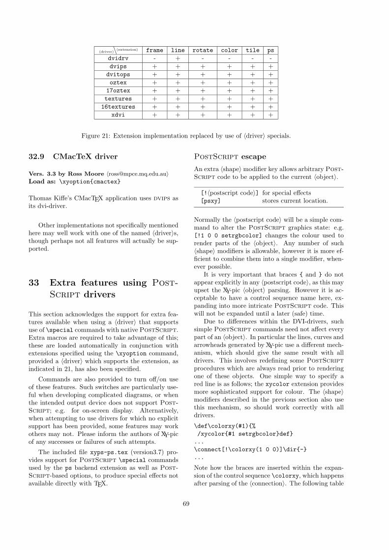
〈driver〉
∖〈extension〉 frame line rotate color tile ps
dvidrv - + - - - -dvips + + + + + +
dvitops + + + + + +oztex + + + + + +
17oztex + + + + + +textures + + + + + +
16textures + + + + + +xdvi + + + + + +
Figure 21: Extension implementation replaced by use of 〈driver〉 specials.
32.9 CMacTeX driver
Vers. 3.3 by Ross Moore 〈[email protected]〉Load as: \xyoption{cmactex}
Thomas Kiffe’s CMacTEX application uses dvips asits dvi-driver.
Other implementations not specifically mentionedhere may well work with one of the named 〈driver〉s,though perhaps not all features will actually be sup-ported.
33 Extra features using Post-
Script drivers
This section acknowledges the support for extra fea-tures available when using a 〈driver〉 that supportsuse of \special commands with native PostScript.Extra macros are required to take advantage of this;these are loaded automatically in conjunction withextensions specified using the \xyoption command,provided a 〈driver〉 which supports the extension, asindicated in 21, has also been specified.
Commands are also provided to turn off/on useof these features. Such switches are particularly use-ful when developing complicated diagrams, or whenthe intended output device does not support Post-
Script; e.g. for on-screen display. Alternatively,when attempting to use drivers for which no explicitsupport has been provided, some features may workothers may not. Please inform the authors of XY-picof any successes or failures of such attempts.
The included file xyps-ps.tex (version3.7) pro-vides support for PostScript \special commandsused by the ps backend extension as well as Post-
Script-based options, to produce special effects notavailable directly with TEX.
PostScript escape
An extra 〈shape〉modifier key allows arbitrary Post-
Script code to be applied to the current 〈object〉.
[!〈postscript code〉] for special effects[psxy] stores current location.
Normally the 〈postscript code〉 will be a simple com-mand to alter the PostScript graphics state: e.g.[!1 0 0 setrgbcolor] changes the colour used torender parts of the 〈object〉. Any number of such〈shape〉 modifiers is allowable, however it is more ef-ficient to combine them into a single modifier, when-ever possible.
It is very important that braces { and } do notappear explicitly in any 〈postscript code〉, as this mayupset the XY-pic 〈object〉 parsing. However it is ac-ceptable to have a control sequence name here, ex-panding into more intricate PostScript code. Thiswill not be expanded until a later (safe) time.
Due to differences within the DVI-drivers, suchsimple PostScript commands need not affect everypart of an 〈object〉. In particular the lines, curves andarrowheads generated by XY-pic use a different mech-anism, which should give the same result with alldrivers. This involves redefining some PostScript
procedures which are always read prior to renderingone of these objects. One simple way to specify ared line is as follows; the xycolor extension providesmore sophisticated support for colour. The 〈shape〉modifiers described in the previous section also usethis mechanism, so should work correctly with alldrivers.
\def\colorxy(#1){%/xycolor{#1 setrgbcolor}def}
...\connect[!\colorxy(1 0 0)]\dir{-}...
Note how the braces are inserted within the expan-sion of the control sequence \colorxy, which happensafter parsing of the 〈connection〉. The following table
69
shows which graphics parameters are treated in thisway, their default settings, and the type of Post-
Script code needed to change them.
colour /xycolor{0 setgray}defline-width /xywidth{.4 setlinewidth}defdashing /xydash{[] 0 setdash}defline-cap /xycap{1 setlinecap}defline-join /xyjoin{1 setlinejoin}def
This feature is meant primarily for modifying therendering of objects specified in TEX and XY-pic, notfor drawing new objects within PostScript. Noguarantee can be given of the current location, orscale, which may be different with different drivers.However a good PostScript programmer will beable to overcome such difficulties and do much more.To aid in this the special modifier [psxy] is providedto record the location where the reference point ofthe current 〈object〉 will be placed. Its coordinatesare stored with keys xyXpos and xyYpos.
33.1 Colour
The included file xyps-c.tex (version 3.7) providesPostScript support for the effects defined in thecolor extension in §13.
This file is loaded and its effects are activatedautomatically whenever \xyoption{color} is re-quested and the current 〈driver〉 supports colours us-ing PostScript. Should there be any need to turnoff this support, the following commands are avail-able; they obey usual TEX groupings.
\NoPScolor remove PostScript support\UsePScolor reinstate PostScript.
Without PostScript support some drivers may stillbe able to provide some support for colours. Thesecommands are not guaranteed to work adequatelywith all drivers. They are provided primarily for test-ing and trouble-shooting; e.g. with 〈driver〉 configu-rations untested by the authors of XY-pic, who shouldbe notified of any difficulties.
33.2 Frames
The included file xyps-f.tex (version 3.7) providesPostScript support for the effects defined in theframe extension described in §9. It implements someeffects otherwise unattainable.
This file is loaded and its effects are activatedautomatically whenever \xyoption{frame} is re-quested and the current 〈driver〉 supports Post-
Script effects for frames. Should there be any need
to turn off this support, the following commands areavailable; they obey usual TEX groupings.
\NoPSframes remove PostScript support\UsePSframes reinstate PostScript.
Without PostScript support ellipses may be shownas circles and all filled regions may be representedas black rectangles. These commands are providedprimarily for testing and trouble-shooting; e.g. with〈driver〉 configurations untested by the authors of XY-pic, who should be notified of any difficulties.
33.3 Line-styles
The included file xyps-l.tex (version 3.7) providesPostScript support for the effects defined in theline extension described in §11.
This file is loaded and its effects are activated au-tomatically whenever \xyoption{line} is requestedand the current 〈driver〉 supports PostScript linestyles. Should there be any need to turn off thissupport, the following commands are available; theyobey usual TEX groupings.
\NoPSlines remove PostScript support\UsePSlines reinstate PostScript.
Without PostScript support lines can be expectedto be displayed in the default style, having thicknessof .4pt. These commands are provided primarily fortesting and trouble-shooting; e.g. with 〈driver〉 con-figurations untested by the authors of XY-pic, whoshould be notified of any difficulties.
33.4 Rotations and scaling
The included file xyps-r.tex (version 3.7) providesPostScript support for the effects defined in therotate extension described in §12.
This file is loaded and its effects are activatedautomatically whenever \xyoption{rotate} is re-quested and the current 〈driver〉 supports Post-
Script rotations. Should there be any need to turnoff this support, the following commands are avail-able; they obey usual TEX groupings.
\NoPSrotate remove PostScript support\UsePSrotate reinstate PostScript.
Without PostScript support diagrams can beexpected to be displayed unrotated and unscaled.These commands are provided primarily for testingand trouble-shooting; e.g. with 〈driver〉 configura-tions untested by the authors of XY-pic, who shouldbe notified of persistent difficulties.
70
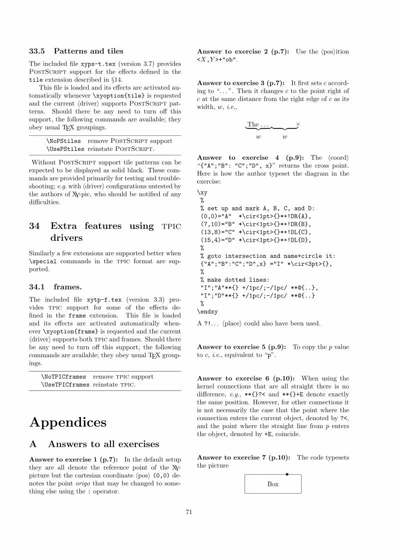
33.5 Patterns and tiles
The included file xyps-t.tex (version 3.7) providesPostScript support for the effects defined in thetile extension described in §14.
This file is loaded and its effects are activated au-tomatically whenever \xyoption{tile} is requestedand the current 〈driver〉 supports PostScript pat-terns. Should there be any need to turn off thissupport, the following commands are available; theyobey usual TEX groupings.
\NoPStiles remove PostScript support\UsePStiles reinstate PostScript.
Without PostScript support tile patterns can beexpected to be displayed as solid black. These com-mands are provided primarily for testing and trouble-shooting; e.g. with 〈driver〉 configurations untested bythe authors of XY-pic, who should be notified of anydifficulties.
34 Extra features using tpic
drivers
Similarly a few extensions are supported better when\special commands in the tpic format are sup-ported.
34.1 frames.
The included file xytp-f.tex (version 3.3) pro-vides tpic support for some of the effects de-fined in the frame extension. This file is loadedand its effects are activated automatically when-ever \xyoption{frame} is requested and the current〈driver〉 supports both tpic and frames. Should therebe any need to turn off this support, the followingcommands are available; they obey usual TEX group-ings.
\NoTPICframes remove tpic support\UseTPICframes reinstate tpic.
Appendices
A Answers to all exercises
Answer to exercise 1 (p.7): In the default setupthey are all denote the reference point of the XY-picture but the cartesian coordinate 〈pos〉 (0,0) de-notes the point origo that may be changed to some-thing else using the : operator.
Answer to exercise 2 (p.7): Use the 〈pos〉ition<X,Y >+"ob".
Answer to exercise 3 (p.7): It first sets c accord-ing to “. . . ”. Then it changes c to the point right ofc at the same distance from the right edge of c as itswidth, w, i.e.,
The . . .︸ ︷︷ ︸w
×︸ ︷︷ ︸w
Answer to exercise 4 (p.9): The 〈coord〉“{"A";"B": "C";"D", x}” returns the cross point.Here is how the author typeset the diagram in theexercise:
\xy%% set up and mark A, B, C, and D:(0,0)="A" *\cir<1pt>{}*+!DR{A},(7,10)="B" *\cir<1pt>{}*+!DR{B},(13,8)="C" *\cir<1pt>{}*+!DL{C},(15,4)="D" *\cir<1pt>{}*+!DL{D},%% goto intersection and name+circle it:{"A";"B":"C";"D",x} ="I" *\cir<3pt>{},%% make dotted lines:"I";"A"**{} +/1pc/;-/1pc/ **@{..},"I";"D"**{} +/1pc/;-/1pc/ **@{..}%
\endxy
A ?!. . . 〈place〉 could also have been used.
Answer to exercise 5 (p.9): To copy the p valueto c, i.e., equivalent to “p”.
Answer to exercise 6 (p.10): When using thekernel connections that are all straight there is nodifference, e.g., **{}?< and **{}+E denote exactlythe same position. However, for other connections itis not necessarily the case that the point where theconnection enters the current object, denoted by ?<,and the point where the straight line from p entersthe object, denoted by +E, coincide.
Answer to exercise 7 (p.10): The code typesetsthe picture
Box
•
71
Answer to exercise 8 (p.11): This does the job,saving each point to make the previous point avail-able for the next piece:
\xy@={(0,-10),(10,3),(20,-5)},s0="prev" @@{;"prev";**@{-}="prev"}
\endxy
Notice how we close the line by first saving s0, thelast point visited, such that the first point will beconnected to it.
Answer to exercise 9 (p.11): The author used
\xy ={.{+DL(2)}.{+UR(2)}}"dbl",*+<3pc,2pc>{+}*\frm{.}, "dbl"*\frm{--}
\endxy
to typeset the figure in the exercise.
Answer to exercise 10 (p.13): The first type-sets “a” centered around 0 and then moves c to thelower right corner, the second typesets “a” above the0 point and does not change c. With a “+” at 0 theylook like this: +a and +a .
Answer to exercise 11 (p.13): They have theoutlines ∑
+ and∑+
because the first is enlarged by the positive offset tothe upper right corner and the second by the negativeoffset to the lower left corner.
Answer to exercise 12 (p.14): The first has noeffect since the direction is set to be that of a vectorin the current direction, however, the second reversesthe current direction.
Answer to exercise 13 (p.15): None in bothcases.
Answer to exercise 14 (p.18): One way is
$$\xy*{+}; p+(6,3)*{+} **{} ?(1)*@{-} *!/-5pt/^\dir{-}*^\dir{-} *!/^-5pt/\dir{-}
\endxy$$
Thus we first create the two +s as p and c andconnect them with the dummy connection **{} tosetup the direction parameters. Then we move ‘ontop of c’ with ?(1) and position the four sides of thesquare using ^ and _ for local direction changes and/〈dimen〉/ for skewing the resulting object by movingits reference point in the opposite direction.
Answer to exercise 15 (p.18): One way is to addextra half circles skewed such that they create the il-lusion of a shade:
$$\xy*\cir<5pt>{}*!<-.2pt,.2pt>\cir<5pt>{dr^ul}*!<-.4pt,.4pt>\cir<5pt>{dr^ul}*!<-.6pt,.6pt>\cir<5pt>{dr^ul}
\endxy$$
Answer to exercise 16 (p.21): This is the codethat was actually used:
\xy (0,20)*[o]+{A};(60,0)*[o]+{B}="B"**\crv{} \POS?(.4)*_+!UR{0},"B"**\crv{(30,30)} \POS?*^+!D{1},"B"**\crv{(20,40)&(40,40)} \POS?*^+!D{2},"B"**\crv{(10,20)&(30,20)&(50,-20)&(60,-10)}\POS?*+^!UR{4} \endxy
Answer to exercise 17 (p.21): This is the codethat was used to typeset the picture:
\xy (0,20)*+{A};(60,0)*+{B}**\crv{(10,20)&(30,20)&(50,-20)&(60,-10)}?<*\dir{<} ?>*\dir{>}?(.65)*{\oplus} *!LD!/^-5pt/{x}?(.65)/12pt/*{\oplus} *!LD!/^-5pt/{x’}?(.28)*=0{\otimes}-/40pt/*+{Q}="q"+/100pt/*+{P};"q" **\dir{-}
\endxy
Answer to exercise 18 (p.21): Here is the codethat was used to typeset the picture:
\def\ssz#1{\hbox{$_{^{#1}}$}}\xy (0,0)*+{A};(30,-10)*+{B}="B",**\dir{-},"B"**\crv{(5,20)&(20,25)&(35,20)}?<(0)*\dir{<}="a" ?>(1)*\dir{>}="h"?(.1)*\dir{<}="b" ?(.9)*\dir{>}="i"?(.2)*\dir{<}="c" ?(.8)*\dir{>}="j"?(.3)*\dir{<}="d" ?(.7)*\dir{>}="k"?(.4)*\dir{<}="e" ?(.6)*\dir{>}="l"?(.5)*\dir{|}="f","a"*!RC\txt{\ssz{(\lt)}};"h"*!LC\txt{\ssz{\;(\gt)}},**\dir{.},
"b"*!RD{\ssz{.1}};"i"*!L{\ssz{\;.9}},**\dir{-},
"c"*!RD{\ssz{.2}};"j"*!L{\ssz{\;.8}},**\dir{-},
"d"*!RD{\ssz{.3}};"k"*!L{\ssz{\;.7}},**\dir{-},
"e"*!RD{\ssz{.4}};"l"*!LD{\ssz{.6}},**\dir{-},
"f"*!D!/^-3pt/{\ssz{.5}}\endxy
72
Answer to exercise 19 (p.26): Here is how:
\xy(0,0) *++={A} *\frm{o} ;(10,7) *++={B} *\frm{o} **\frm{.}
\endxy
Answer to exercise 20 (p.26): The *\cir {} op-eration changes c to be round whereas *\frm {o}does not change c at all.
Answer to exercise 21 (p.26): Here is how:
\xy(0,0) *+++{A} ;(10,7) *+++{B} **\frm{.}**\frm{^\}} ; **\frm{_\}}
\endxy
The trick in the last line is to ensure that the ref-erence point of the merged object to be braced is theright one in each case.
Answer to exercise 22 (p.30): This is how theauthor specified the diagram:
\UseCrayolaColors\xy\drop[*1.25]\xybox{\POS(0,0)*{A};(100,40)*{B}**{}?<<*[@_][red][o]=<5pt>{\heartsuit};?>>>*[@_][Plum][o]=<3pt>{\clubsuit}**[|*][|.5pt][thicker]\dir{-},
?(.1)*[left]!RD\txt{label 1}*[red]\frm{.}?(.2)*[!gsave newpath
xyXpos xyYpos moveto 50 dup rlineto20 setlinewidth 0 0 1 setrgbcolor strokegrestore][psxy]{.},
?(.2)*[@]\txt{label 2}*[red]\frm{.},?(.2)*[BurntOrange]{*},?(.3)*[halfsize]\txt{label 3}*[red]\frm{.}?(.375)*[flip]\txt{label 4}*[red]\frm{.}?(.5)*[dblsize]\txt{label 5}*[red]\frm{.}?(.5)*[WildStrawberry]{*},?(.7)*[hflip]\txt{label 6}*[red]\frm{.}?(.8)*[vflip]\txt{label 7}*[red]\frm{.}?(.9)*[right]!LD\txt{label 8}*[red]\frm{.}?(.5)*[@][*.66667]!/^30pt/\txt{special effect: aligned text}*[red]\frm{.}
}\endxy
Answer to exercise 23 (p.40): Here is what theauthor did:
\xy *+{A}*\cir<10pt>{}="me"\PATH ‘ul^ur,"me" "me" |>*:(1,-.25)\dir{>}
\endxy
The trick is getting the arrow head right: the :modifier to the explicit \dir 〈object〉 does that.
Answer to exercise 24 (p.40): The author did
\xy(0,0)\ar @{-->} (30,7) ^A="a"\POS(10,12)*+\txt{label} \ar "a"
\endxy
Answer to exercise 25 (p.41): Here is the entireXY-picture of the exercise:
\xy ;<1pc,0pc>:\POS(0,0)*+{A}\ar +(-2,3)*+{A’}*\cir{}\ar @2 +( 0,3)*+{A’’}*\cir{}\ar @3 +( 2,3)*+{A’’’}*\cir{}\POS(6,0)*+{B}\ar @1{||.>>} +(-2,3)*+{B’}*\cir{}\ar @2{||.>>} +( 0,3)*+{B’’}*\cir{}\ar @3{||.>>} +( 2,3)*+{B’’’}*\cir{}
\endxy
The first batch use the default {->} specification.
Answer to exercise 26 (p.42): The author used
\newdir{ >}{{}*!/-5pt/\dir{>}}
Answer to exercise 27 (p.42): The author used
\xy\ar @{>>*\composite{\dir{x}*\dir{+}}<<}(20,7)
\endxy
Answer to exercise 28 (p.42): The author used
\xy *{\circ}="b" \ar@(ur,ul) c\ar@{.>}@(dr,ul) (20,0)*{\bullet}
\endxy
Note that it is essential that the curving specificationcomes after the arrow style.
Answer to exercise 29 (p.46): Here is the codeused to typeset the pasting diagram in figure 15.
\xymatrixrowsep{1.5pc}\xymatrixcolsep{3pc}\diagram&&\relax\rtwocell<0>^{f_3^{}\;\;}{\omit}&\relax\ddtwocell<0>{\omit}\drtwocell<0>^{\;\;f_4^{}}{<3>}\ddrrtwocell<\omit>{<8>}\\
&&&&\relax\drtwocell<0>^{\;\;f_5^{}}{\omit}\\A \uurrlowertwocell<-6>{\omit}\relax\uurrcompositemap<2>_{f_1^{}}^{f_2^{}}{<.5>}
73
\drtwocell<0>_{g_1^{}\;}{\omit}&&&\relax\urtwocell<0>{\omit}&&\relax\rtwocell<0>^{f_6^{}\;}{\omit}&\relax\rlowertwocell<-3>_{g_4^{}}{<-1>}\rcompositemap<6>_{f_7^{}}^{f_8^{}}{\omit}& B \\&\relax\urrtwocell<0>{\omit}\xcompositemap[-1,4]{}%<-4.5>_{g_2^{}}^{g_3^{}}{\omit}\\
\enddiagram
For the straight arrows, it would have been simplerto use \..to provided xyarrow has been loaded. In-stead \..twocell<0>...{\omit } was used to illus-trate the versatility of nudging and \omit ; thusxy2cell can completely handle a wide range of di-agrams, without requiring xyarrow. Note also theuse of \relax at the start of each new cell, to avoidpremature expansion of a complicated macro, whichcan upset the compiling mechanism.
Answer to exercise 30 (p.47): Here is the codeused by the author to set the first diagram.
{\uppercurveobject{{?}}\lowercurveobject{{\circ}}
\xymatrixcolsep{5pc}\xymatrixrowsep{2pc}\diagram\relax\txt{ FUn }\rtwocell<8>{!\&}& \relax\txt{ gaMES }\enddiagram}
Here is the code used for the second diagram.
\xymatrixcolsep{2.5pc}\xymatrixrowsep{4pc}\diagram\relax\txt<1.5cm>{\bf Ground State}\rrtwocell<12>~^{+{}~**!/-2.5pt/\dir{>}}~_{++{}~**!/5pt/\dir{<<}}^{<1.5>\txt{\small continuous power}}_{<1.5>\txt{\small pulsed emission}}{!}
& \relax\;\; N\!i\,C\!d\;\; \Circled& \relax\txt<1.50cm>{\bf Excited State}\enddiagram
Answer to exercise 31 (p.50): The author did
\xymatrix @!=1pc {**[l] A\times B
\ar[r]^{/A} \ar[d]_{/B}& B \ar[d]^{\times A}
\\A \ar[r]_{B\times}& **[r] B\times A
}
Answer to exercise 32 (p.50): Modifiers areused to make all entries round with a frame – thegeneral form is used to ensure that the sequence iswell-defined. Finally the matrix is rotated to make itpossible to enter it as a simple square:
\entrymodifiers={=<1pc>[o][F-]}\xymatrix @ur {A \save[];[r] **\dir{-},
[];[dr]**\dir{-},[];[d] **\dir{-}\restore
& B \\C & D }
Answer to exercise 33 (p.51): Here is how:
\xymatrix @W=3pc @H=1pc @R=0pc @*[F-] {%: \save+<-4pc,1pc>*\hbox{\it root}
\ar[]\restore
\\{\bullet}
\save*{}\ar‘r[dd]+/r4pc/‘[dd][dd]
\restore\\{\bullet}
\save*{}\ar‘r[d]+/r3pc/‘[d]+/d2pc/
‘[uu]+/l3pc/‘[uu][uu]\restore
\\1 }
Answer to exercise 34 (p.52): The first A wasnamed to allow reference from the last:
\xygraph{[]A="A1" :@/^/ [r]A
:@/^/ [r]A:@/^/ "A1" }
Answer to exercise 35 (p.53): The author did
\SelectTips{cm}{}\objectmargin={1pt}\xygraph{ !{0;(.77,-.77):0}!~:{@{-}|@{>}}w (:[r(.6)]{x_1}
,:[d]z:[r]y:[u(.6)]{x_2}:"x_1":"z":@( {"w";"z"}, {"y";"z"})"z":"x_2") }
It also shows that one can use {}s inside delimitedarguments provided one adds a space to avoid the {}sbeing shaved off!
74
Answer to exercise 36 (p.54): Here is the codeactually used to typeset the \xypolygon s, within an\xygraph . It illustrates three different ways to placethe numbers. Other ways are also possible.
\def\objectstyle{\scriptscriptstyle}\xy \xygraph{!{/r2pc/:}[] !P3"A"{\bullet}"A1"!{+U*++!D{1}} "A2"!{+LD*+!RU{2}}"A3"!{+RD*+!LU{3}} "A0"[rrr]*{0}*\cir<5pt>{}!P6"B"{~<-\cir<5pt>{}}"B1"1 "B2"2 "B3"3 "B4"4 "B5"5 "B6"6 "B0"[rrr]0 !P9"C"{~*{\xypolynode}}}\endxy
B Version 2 Compatibility
Vers. 3.4 by Kristoffer H. Rose 〈[email protected]〉Load as: \xyoption{v2}
This appendix describes the special backwards com-patibility with XY-pic version 2: diagrams written ac-cording to the “Typesetting diagrams with XY-pic:User’s Manual” [13] should typeset correctly with thisloaded. The compatibility is available either as anXY-option or through the special files xypic.sty andxypic.tex described below.
There are a few exceptions to the compatibility:the features described in §B.1 below are not providedbecause they are not as useful as the author originallythought and thus virtually never used. And one extracommand is provided to speed up typesetting of doc-uments with XY-pic version 2 diagrams by allowingthe new compilation functionality with old diagrams.
The remaining sections list all the obsolete com-mands and suggest ways to achieve the same thingsusing XY-pic 3.7, i.e., without the use of this option.They are grouped as to what part of XY-pic replacesthem; the compilation command is described last.
Note: “version 2” is meant to cover all publicreleases of XY-pic in 1991 and 1992, i.e., version 1.40and versions 2.1 through 2.6. The published manualcited above (for version 2.6) is the reference in caseof variations between these versions, and only thingsdocumented in that manual will be supported by thisoption!19
B.1 Unsupported incompatibilities
Here is a list of known incompatibilities with version2 even when the v2 option is loaded.
• Automatic ‘shortening’ of arrow tails using |<<breaks was a bug and has been ‘fixed’ so it doesnot work any more. Put a |<\hole break beforeit.
• The version 2.6 * position operator is not avail-able. The version 2.6 construction t0;t1*(x,y)should be replaced by the rather long but equiv-alent construction
{ t0 ;p+/r/: t1 ="1";p+/u/,x;(0,0);:"1";p+/r/,y;(0,0);:: (x,y)}
In most cases t0;t1**{}?(x), possibly with atrailing +/^ . . . /, suffices instead.
• Using t0;t1:(x,y) as the target of an arrowcommand does not work. Enclose it in braces,i.e., write
{ t0 ; t1 :(x,y)}
• The older \pit, \apit, and \bpit commandsare not defined. Use \dir{>} (or \tip) withvariants and rotation.
• The even older notation where an argument inbraces to \rto and the others was automati-cally taken to be a ‘tail’ is not supported. Usethe supported |<. . . notation.
If you do not use these features then your version 2(and earlier) diagrams should typeset the same withthis option loaded except that sometimes the spac-ing with version 3 is slightly different from that ofversion 2.6 which had some spacing bugs.
B.2 Obsolete kernel features
The following things are added to the kernel by thisoption and described here: idioms, obsolete positions,obsolete connections, and obsolete objects. For eachwe show the suggested way of doing the same thingwithout this option:
Removed AMS-TEX idioms
Some idioms from AMS-TEX are no longer usedby XY-pic: the definition commands \defineand \redefine, and the size commands \dsize,\tsize, \ssize, and \sssize. Please usethe commands recommended for your format—forplain TEX these are \def for the first two and\displaystyle, \textstyle, \scriptstyle, and\scriptscriptstyle for the rest. The v2 option en-sures that they are available anyway.
Version also 2 used the AMS-TEX \text anda (non-object) box construction \Text which areemulated—\text is only defined if not already de-fined, however, using the native one (of AMS-TEX orAMS-LATEX or whatever) if possible. Please use the\txt object construction described in §6.3 directlysince it is more general and much more efficient!
19In addition a few of the experimental facilities supported in v2.7–2.12 are also supported.
75
Obsolete state
Upto version 2.6 users could access the state variables\cL, \cR, \cH, and \cD, which are defined.
From v2.7 to 2.12 users could use the namesof the state \dimen registers \Xmin, \Xmax, \Ymin,and \Ymax; \Xp, \Yp \Dp, \Up, \Lp, and \Rp; \Xc,\Yc \Dc, \Uc, \Lc, and \Rc; \Xorigin, \Yorigin,\Xxbase, \Yxbase, \Xybase, and \Yybase. Now thesame effect can be achieved using 〈corner〉s but v2defines the aliases.
Obsolete position manipulation
In version 2 many things were done using individual〈decor〉 control sequences that are now done using〈pos〉 operators.
Version 2 positioning Replacement
\go〈pos〉 \POS;p,〈pos〉\aftergo{〈decor〉}〈pos〉
\afterPOS{〈decor〉};p,〈pos〉\merge \POS.p\relax\swap \POS;\relax\Drop{〈text〉} \drop+{〈text〉}
Obsolete connections
These connections are now implemented using direc-tionals.
Version 2 connection Replacement
\none \connect h\dir{}\solid \connect h\dir{-}\Solid \connect h\dir2{-}\Ssolid \connect h\dir3{-}\dashed \connect h\dir{--}\Dashed \connect h\dir2{--}\Ddashed \connect h\dir3{--}\dotted \connect h\dir{.}\Dotted \connect h\dir2{.}\Ddotted \connect h\dir3{.}\dottedwith{〈text〉} \connect h{〈text〉}
Note how the ‘hidden’ specifier h should be used be-cause version 2 connections did not affect the size ofdiagrams.
Obsolete tips
These objects all have \dir-names now:
Version 2 tip Replacement
\notip \dir{}\stop \dir{|}
\astop \dir^{|}\bstop \dir_{|}\tip \dir{>}\atip \dir^{>}\btip \dir_{>}\Tip \dir2{>}\aTip \object=<5pt>:(32,-1)\dir^{>}\bTip \object=<5pt>:(32,+1)\dir_{>}\Ttip \dir3{>}\ahook \dir^{(}\bhook \dir_{(}\aturn \dir^{’}\bturn \dir_{’}
The older commands \pit, \apit, and \bpit, arenot provided.
Obsolete object constructions
The following object construction macros are madeobsolete by the enriched 〈object〉 format:
Version 2 object Replacement
\rotate(〈factor〉)〈tip〉\object:(〈factor〉,〈factor〉){〈tip〉}
\hole \object+{}\squash〈tip〉 \object=0{〈tip〉}\grow〈tip〉 \object+{〈tip〉}\grow<〈dimen〉>〈tip〉 \object+<〈dimen〉>{〈tip〉}\squarify{〈text〉} \object+={〈text〉}\squarify<〈dimen〉>{〈text〉}
\object+=<〈dimen〉>{〈text〉}
where rotation is done in a slightly different mannerin version 3.7 (it was never accurate in version 2).
B.3 Obsolete extensions & features
Version 2 had commutative diagram functionalitycorresponding to the frames extension and parts ofthe matrix and arrow features. These are thereforeloaded and some extra definitions added to emulatecommands that have disappeared.
Frames
The version 2 frame commands are emulated us-ing the frame extension (as well as the \dotframed,\dashframed, \rounddashframed commands comm-unicated to some users by electronic mail):
Version 2 object Replacement
\framed \drop\frm{-}\framed<〈dimen〉> \drop\frm<〈dimen〉>{-}\Framed \drop\frm{=}\Framed<〈dimen〉> \drop\frm<〈dimen〉>{=}
76
\dotframed \drop\frm{.}\dashframed \drop\frm{--}\rounddashframed \drop\frm{o-}\circled \drop\frm{o}\Circled \drop\frm{oo}
Matrices
The \diagram 〈rows〉 \enddiagram command is pro-vided as an alias for \xymatrix{ 〈rows〉 } centeredin math mode and \LaTeXdiagrams changes it to use\begin . . . \end syntax. v2 sets a special internal‘old matrix’ flag such that trailing \\ are ignored andentries starting with * are safe.
\NoisyDiagrams is ignored because the matrixfeature always outputs progress messages.
Finally the version 2 \spreaddiagramrows,\spreaddiagramcolumns spacing commandsare emulated using \xymatrixrowsep and\xymatrixcolsep:
Arrows
The main arrow commands of version 2 were the\morphism and \definemorphism commands whichnow have been replaced by the \ar command.
v2 provides them as well as uses them to definethe version 2 commands \xto, \xline, \xdashed,\xdotted, \xdouble, and all the derived commands\dto, \urto, . . . ; the \arrow commands of the β-releases of v3 is also provided.
Instead of commands like \rrto and \uldoubleyou should use the arrow feature replacements\ar[rr] and \ar@{=}[ul].
The predefined turning solid arrows \lltou, . . . ,\tord are defined as well; these are now easy to dowith 〈turn〉s.
B.4 Obsolete loading
The v2 User’s Manual says that you can load XY-picwith the command \input xypic and as a LATEX 2.09‘style option’ [xypic]. This is made synonymouswith loading this option by the files xypic.tex andxypic.sty distributed with the v2 option.
xypic.tex: This file (version 3.3) just loads the v2feature.
xypic.sty: Loads xy.sty and the v2 feature.
B.5 Compiling v2-diagrams
In order to make it possible to use the new compila-tion features even on documents written with XY-pic
v2, the following command was added in v2.12:
\diagramcompileto{ 〈name〉 } . . . \enddiagram
which is like the ordinary diagram command exceptthe result is compiled (see note 5e). Note that com-pilation is not quite safe in all cases!
There is also the following command that switcheson automatic compilation of all diagrams createdwith the v2 \diagram . . . \enddiagram command:
\CompileAllDiagrams { 〈prefix〉 }\NoCompileAllDiagrams\ReCompileAllDiagrams
will apply \xycompileto{〈prefix〉n}{. . . } to each di-agram with n a sequence number starting from 1. Use\CompileMatrices and \CompilePrefix instead!
If for some reason a diagram does not work whencompiled then replace the \diagram command with\diagramnocompile (or in case you are using theLATEX form, \begin{diagramnocompile}).
C Common Errors
In this appendix we describe some common caseswhere small mistakes in XY-pictures result in TEX er-ror messages that may seem cryptic.
! Box expected.! A 〈box〉 was supposed to be here. This mes-sage is common when an XY-pic 〈object〉 is mistypedsuch that XY-pic expects but does not find a TEX〈box〉 construction.
! LaTeX Error: Bad math environment delim-iter.! File ended while scanning use of \xycompiled.! Argument of \codeof@ has an extra }. Theseerrors can happen while reading an incomplete com-piled picture (such a beast is created when XY-piccrashes during compilation due to a syntax error orother such problem).
! Missing } inserted. This happens when \endxywas left out.
To Do: Also include the more obscure ones. . .
77
References
[1] Adobe Systems Incorporated. PostScript Lan-guage Reference Manual, second edition, 1990.
[2] American Mathematical Society. AMS-LATEXVersion 1.1 User’s Guide, 1.1 edition, 1991.
[3] Karl Berry. Expanded plain TEX, version 2.6 edi-tion, May 1994. Available for anonymous ftpfrom CTAN in macros/eplain/doc.
[4] Michel Goossens, Frank Mittelbach, and Alexan-der Samarin. The LATEX Companion. Addison-Wesley, 1994.
[5] Brian W. Kernighan. PIC—a language for type-setting graphics. Software Practice and Experi-ence, 12(1):1–21, 1982.
[6] Donald E. Knuth. The TEXbook. Addison-Wesley, 1984.
[7] Donald E. Knuth. Computer Modern Typefaces,volume A of Computers & Typesetting. Addison-Wesley, 1986.
[8] Leslie Lamport. LATEX—A Document Prepara-tion System. Addison-Wesley, 1986.
[9] Leslie Lamport. LATEX—A Document Prepara-tion System. Addison-Wesley, 2nd edition, 1994.
[10] P. Naur et al. Report on the algorithmic lan-guage ALGOL 60. Communications of the ACM,3:299–314, 1960.
[11] Tomas Rokicki. DVIPS: A TEX Driver. Dis-tributed with the dvips program found on CTANarchives.
[12] Kristoffer H. Rose. How to typeset pretty dia-gram arrows with TEX—design decisions used inXY-pic. In Jirı Zlatuska, editor, EuroTEX ’92—Proceedings of the 7th European TEX Con-ference, pages 183–190, Prague, Czechoslo-vakia, September 1992. Czechoslovak TEX UsersGroup.
[13] Kristoffer H. Rose. Typesetting diagrams withXY-pic: User’s manual. In Jirı Zlatuska, edi-tor, EuroTEX ’92—Proceedings of the 7th Eu-ropean TEX Conference, pages 273–292, Prague,Czechoslovakia, September 1992. CzechoslovakTEX Users Group.
[14] Kristoffer H. Rose. XY-pic User’s Guide. DIKU,University of Copenhagen, Universitetsparken 1,DK–2100 København Ø, 3.0 edition, June 1995.
[15] Kristoffer H. Rose and Ross R. Moore. XY-pic complete sources with TEXnical commentary.not yet available, June 1995.
[16] Michael D. Spivak. The Joy of TEX—A GourmetGuide to Typesetting with the AMS-TEX MacroPackage. American Mathematical Society, sec-ond edition, 1990.
[17] TUG Working Group TWG-TDS. A directorystructure for TEX files version 0.98. URL, May1995. Available with URL ftp://jasper.ora.com/pub/twg-tds/.
Index
!, 8&, 48’, 39(), 8(0), 8(0,0), 71(1), 8*, 8, 39, 40, 42, 48, 50, 75**, 8, 40, 50+, 8,, 8, 40-, 8, 39., 8.xyd, 15/, 38, 39, 42//, 8:, 8, 12
::, 8;, 8<, 8, 38–40<>, 8<>(.5), 39=, 8, 38–40>, 8, 38–40?, 8, 40@, 8, 39, 41, 49@!, 41, 49@!0, 50@!=, 50@!C, 49@!R, 49@(, 10, 41, 42@), 10@*, 41, 50
@+, 10@-, 10@/, 41, 42@1, 50@<, 41, 43@=, 10@?, 41, 43@@, 10@C, 49@H, 50@L, 50@M, 50@R, 49@W, 50@‘, 41@i, 10[.], 13
78

[=, 12, 14, 30, 33[P:, 37[], 13[c], 14[d], 14[dvips], 5[l], 14[o], 13[r], 14[textures], 5[u], 14\\, 48^, 39–41_, 39–41‘, 39‘s, 66|, 39, 41|<<, 75~, 39
0, 6, 8, 411, 412, 413, 4110, 2711, 2712, 27
a, 8active characters, 4〈add op〉, 12\aftergo , 76\afterPATH , 38\afterPOS , 15, 16, 39\ahook , 76allocation, 5AMS-LATEX, 5, 15AMS-TEX, 5\apit , 75\ar , 14, 38, 66array, 51arrow head, 41arrow stem, 41arrow tail, 41\astop , 76\aTip , 76\atip , 76\aturn , 76
banner, 5\bhook , 76BNF, 4〈body of the option〉, 19\bpit , 75\bstop , 76\bTip , 76\btip , 76\bturn , 76
C, 8, 10c, 6c, 8cartesian coordinate system, 6category code, 4CD, 8\cD , 76\cH , 76〈cir〉, 19\cir , 18, 73\Circled , 77\circled , 77circles, 5CL, 8\cL , 76cm, 27\Col , 51column spacing, 49〈command〉, 16\CompileFixPoint , 15\CompilePrefix , 15compiling, 15〈composite〉, 12\composite , 12, 13, 18connect, 6\connect , 16〈coord〉, 8, 37COPYING, 4copyright, 3〈corner〉, 8CR, 8\cR , 76CU, 8current object style, 12, 14
D, 6D, 8, 10Dc, 6Dp, 6\Dashed , 76\dashed , 76dashes, 5\dashframed , 77\Dc , 76\Ddashed , 76\Ddotted , 76〈decor〉, 16decoration, 6default entry, 50\define , 75\definemorphism , 77〈diag〉, 12\diagram , 77dimension registers, 5\dir , 16, 18, 41, 42〈direction〉, 12\documentclass , 5
\dotframed , 77\Dotted , 76\dotted , 76\dottedwith , 76\Dp , 76〈driver〉, 20\Drop , 76\drop , 16\dsize , 75\dumpPSdict {<filename>},
36
E, 8, 10Edge, 6Edgec, 6Edgep, 6\enddiagram , 77\endxy , 6, 15entry height, 50entry margin, 50entry width, 50\entrymodifiers , 50Error, 5〈escape〉, 52eu, 27\everyentry , 51extension, 20extents, 6e|, 37
fixed grid, 49fonts, 5format dependencies, 5formats, 5\Framed , 76\framed , 76free software, 3french.sty, 4\frm , 10, 24\frm {**}, 26\frm {*}, 26
german.sty, 4GNU General Public License, 3\go , 76〈graph〉, 52\grow , 76
h, 12\halfrootthree , 7\halfroottwo , 7\halign , 51\hbox , 12\hole , 40, 76hooks, 5
i, 12idioms, 5\input xy, 4
79

\input xypic, 77
\jot , 9
L, 6L, 8, 10Lc, 6Lp, 6label separation, 50\labelbox , 40\labelmargin , 40\labelstyle , 40LATEX, 5\LaTeXdiagrams , 77LATEX 2ε, 5\Lc , 76LD, 8license, 3〈list〉, 52loading, 4, 5logo, 5\Lp , 76LU, 8
\makeatletter , 4\makeatother , 4\MakeOutlines , 15math mode, 6〈matrix〉, 48matrix, 48matrix orientation, 49matrix spacing, 49\merge , 76messages, 5〈modifier〉, 12, 37\morphism , 77〈move〉, 52movie, 34\MovieSetup , 34\MultipleDrivers , 20
\newdir , 18, 41\newgraphescape , 53\newxycolor , 30\newxypattern , 31\next , 4〈node〉, 52\NoisyDiagrams , 77\none , 76\NoOutlines , 16\NoPSspecials , 35\NoRules , 18\notip , 76\NoTips , 27
〈object〉, 12object, 6\object , 12, 16〈objectbox〉, 12
\objectbox , 11, 40\objectheight , 13\objectmargin , 13, 40\objectwidth , 13\OnlyOutlines , 15〈orient〉, 19orientation, 49
P, 8, 10p, 6p, 8package, 5\partroottwo , 7\PATH , 38\PATHaction , 38\PATHafterPOS , 39\pit , 75〈place〉, 8placement state, 7plainTEX, 5〈pos〉, 8\POS , 16, 38positions, 6privacy, 4
q, 12
R, 6R, 8, 10Rc, 6Rp, 6〈radius〉, 19\Rc , 76RD, 8\redefine , 75redefined, 4\relax , 4, 16\restore , 16\rotate , 76\rounddashframed , 77\Row , 51row spacing, 49\Rp , 76RU, 8
s, 8\save , 16\scene , 34\SelectTips , 27\ShowOutlines , 15\SilentMatrices , 48〈size〉, 12〈slide〉, 8\Solid , 76\solid , 76spacing, 49\spreaddiagramcolumns , 77\spreaddiagramrows , 77
\squarify , 76\squash , 76squiggles, 5\ssize , 75\Ssolid , 76\sssize , 75state, 7〈step〉, 52\stop , 76style, 14style option, 5\swap , 76system dependencies, 5
TEX reference point, 6\Text , 75\text , 75\Tip , 76\tip , 76tips, 5\tsize , 75\Ttip , 76〈turn〉, 66\turnradius , 40\txt , 18
U , 6U, 8, 10Uc, 6Up, 6\Uc , 76\Up , 76\UseCrayolaColors , 30\usepackage , 5\UsePSheader {<filename>},
36\UsePSheader {}, 36\UsePSspecials {}, 35\UseRules , 18\UseSingleDriver , 20\UseTips , 27
v, 12〈vector〉, 8version, 5
Warning, 5warning messages, 4warranty, 3
X, 6x, 8, 9Xorigin , 6Xxbase , 7Xybase , 7Xc, 6Xp, 6Xmax, 6Xmin, 6
80

\Xc , 76\xdashed , 77\xdotted , 77\xdouble , 77\xline , 77\Xmax , 76\Xmin , 76\Xorigin , 76\Xp , 76\xto , 77\Xxbase , 76xy, 27\Xy , 5\xy , 6, 7, 15XY-pic, 5XY-picture state, 6xy.sty, 5xyatip10, 5\xyatipfont , 5\Xybase , 76\xybox , 12xybsql10, 5\xybsqlfont , 5xybtip10, 5\xybtipfont , 5
xycirc10, 5\xycircfont , 5\xycompile , 15, 16\xycompileto , 16xydash10, 5\xydashfont , 5\xydate , 5\xyecho , 15\xyendinput , 19\xyeveryrequest , 19\xyeverywithoption , 19\xygraph , 51xyidioms.tex, 5\xyignore , 16\xymatrix , 14, 48\xymatrixcompile , 49\xymatrixnocompile , 49\xyoption , 5, 19xypic.sty, 77xypic.tex, 77\xyprovide , 19\xyPSdefaultdict , 36\xyquiet , 15, 16xyrecat.tex, 4\xyReloadDrivers , 20
\xyrequire , 19\xyShowDrivers , 20\xytracing , 15, 16\xyverbose , 15, 16\xyversion , 5\xywithoption , 19
Y , 6y, 8, 9Yorigin , 6Yxbase , 7Yybase , 7Yc, 6Yp, 6Ymax, 6Ymin, 6\Yc , 76\Ymax , 76\Ymin , 76\Yorigin , 76\Yp , 76\Yxbase , 76\Yybase , 76
zero position, 6
81