XVA Analysis From the Balance Sheet

Claudio Albanese1,2 and Stephane Crepey3

January 21, 2017

Abstract

In the aftermath of the financial crisis, regulators launched a major effort ofbanking reform aimed at securing the financial system by raising collateralisationand capital requirements. Notwithstanding finance theories, according to whichcosts of capital and of funding for collateral are irrelevant to investment decisions,banks have introduced an array of XVA metrics to precisely quantify them. Inparticular, the KVA (capital valuation adjustment) is emerging as a metric of keyrelevance.

We introduce a capital structure model acknowledging the impossibility for abank to replicate jump-to-default related cash flows. Because of this counterpartycredit risk incompleteness, deals trigger wealth transfers from bank shareholdersto bank creditors and shareholders need to set capital at risk. On this basis wedevise a theory of XVAs, whereby so-called contra-liabilities and cost of capitalare sourced from bank clients at trade inceptions, on top of the fair valuation ofcounterparty credit risk, in order to compensate shareholders for wealth transfersand risk on capital.

Keywords: Counterparty credit risk, jump-to-default risk, market incompleteness,capital structure of a bank, wealth transfer, risk margin, cost of capital, capital valu-ation adjustment (KVA).

Mathematics Subject Classification: 60G44, 91B25, 91B26, 91B30, 91B70, 91B74,91G20, 91G40, 91G60, 91G80.

JEL Classification: C63, D52, D53, G01, G13, G21, G24, G28, G33, M41, P12.

1 Global Valuation Ltd, London.2 CASS School of Business, London.3 Universite d’Evry Val d’Essonne, Laboratoire de Mathematiques et Modelisation d’Evry and UMR

CNRS 8071.Acknowledgement: We are grateful to Agostino Capponi and Karl-Theodor Eisele for comments

and discussions. The research of Stephane Crepey benefited from the support of the “Chair Markets inTransition”, Federation Bancaire Francaise, of the ANR project 11-LABX-0019 and of the EIF grant“Collateral management in centrally cleared trading”.

1

1 Introduction

In the aftermath of the financial crisis, banking regulators launched a major reformeffort aimed at reducing counterparty credit risk by raising collateralisation and capitalrequirements and by incentivising central clearing. The Basel III Accord has beenimplemented in law in most jurisdictions and is being followed by a stream of otherregulatory reforms such as the fundamental review of the trading book (FRTB, seeBCBS (2013)), initial margin for uncleared trades (BCBS 261) and standards to ensuretotal loss-absorbing capacity beyond equity capital (TLAC). Key to the intent of theregulator is the consideration that, assuming complete markets, the level of capital andfunding requirements are irrelevant to all investment decisions, including ask prices forcontingent claims.

On a parallel and independent track, the regulatory framework for the insuranceindustry has also been reformed, but on the basis of a different set of principles. In-surance claims are largely unhedgeable and markets are intrinsically incomplete. Inparticular, the cost of capital is material and is reflected in entry prices. The Swiss Sol-vency Test (2004), followed by Solvency II for the EU, focus on regulating dividenddistribution policies, so as to ensure a sustainable risk remuneration to the shareholdersover the lifetime of the portfolio.

Similar to insurance portfolios, cost of capital also plays a key role for derivativeportfolios. In addition, since banks are intrinsically leveraged, costs of funding strate-gies also matter, whose effect is amplified by the onerous collateralization incentivesand requirements in Basel III. The unintended consequence of Basel III is that banksreacted by pricing into contingent claims the effects of market incompleteness throughso-called XVA metrics, where VA stands for valuation adjustment and X is a catch-allletter to be replaced by C for credit, D for debt, F for funding, M for margin, K forcapital and so on.

Counterparty credit risk incompleteness invalidates several of the conclusions ofModigliani-Miller theory but not all. The purpose of this article is to explain andamend the banking XVA metrics from the point of view of a capital structure modelacknowledging the impossibility for a bank to replicate jump-to-default related cashflows. This outlines the foundation for a hybrid between Basel III and Solvency II,extending the treatment of counterparty credit risk in Basel III to incorporate cost offunding and of capital consistent with the principles of Solvency II.

Our approach results in an economically sustainable XVA methodology, in twosteps. First, the so-called contra-assets are valued as the expected costs of the coun-terparty credit risk related expenses, i.e. the expected costs of counterparty defaultlosses and funding expenditures. Second, on top of these expected costs, a KVA riskpremium is computed as the cost of a sustainable remuneration of the shareholdercapital at risk earmarked to absorb the exceptional (beyond expected) losses.

Pricing approaches in incomplete markets include utility indifference, risk min-imisation and minimal martingale measures, utility maximisation and minimisationover martingale measures, good-deal pricing, market-consistent valuation, probabilitydistortions, among others (see e.g. Schweizer (2001), Rogers (2001), Cochrane andSaa-Requejo (2000) or Madan (2015)). We follow a cost of capital approach because,thanks to the afore-mentioned two-step procedure, it is the only one that can be im-plemented in practice at the level of a realistic bank portfolio, as required for XVApurposes.

A cost of capital approach applied to the counterparty credit risk of the derivative

2

portfolio of a bank raises interesting questions, because of a wealth transfer involvedin the first step and of a dynamic perspective required in the second step. The maincontributions of this work are a clean concept of the KVA, which is the big issue ininvestment banks today but lacks serious academic foundation, as well as the justifica-tion, based on market incompleteness considerations, that the right counterparty riskcorrection to derivative entry prices should be CVA+FVA+KVA, rather than a varietyof other “VA combinations” (e.g. including DVA) that have been floating around inthe literature and in the financial regulation in the last five years.

1.1 Overview of the Paper

A bank is a defaultable entity with shareholders and creditors. Shareholders have thecontrol of the bank and are solely responsible for investment decisions up until thetime of bank default. At default time, shareholders are wiped out. Creditors howeverhave no decision power until the time of default, but are protected by laws such aspari-passu forbidding certain trades that would trigger wealth transfers from them toshareholders.

Counterparty credit risk is related to cash flows or valuations linked to either coun-terparty default or the default of the bank itself. It has capital structure implicationsand is perceived differently by shareholders and creditors. The risk of financial loss asa consequence of client default is hard to replicate since single name CDS instrumentsare illiquid and are typically written on bonds, not on swaps with rapidly varyingvalue. The possibility for the bank of hedging its own default is even more question-able since, in order to hedge it, a bank would need to be able to freely trade its owndebt. But banks are special firms in that they are intrinsically leveraged and cannotbe transformed into a pure equity entity. There is also an argument of scale: Bankliabilities are overwhelming with respect to all other wealth numbers. Last, even if thebank was free to redeem all its debt, bank shareholders could not effectively monetisethe hedging benefit, which would be hampered by bankruptcy costs.

Because of this counterparty credit risk incompleteness, deals trigger wealth trans-fers from bank shareholders to bank creditors and shareholders need to set capital atrisk. On this basis we frame a theory of XVAs, whereby so-called contra-liabilities andcost of capital are sourced from bank clients at trade inceptions, on top of the fairvaluation of counterparty credit risk, in order to compensate shareholders for thesewealth transfers and for the risk on their capital.

We monitor wealth transfer flows across the capital structure of banks and derivethe implications to pricing. By so doing, we propose a fundamental shift from a bank-centric view of derivative valuation to a shareholder view. One can mention the relatedcorporate finance notion of debt overhang in Myers (1977), by which a project valuablefor the firm as a whole may be rejected by shareholders because the project is mainlyvaluable to creditors. But such considerations were never considered in the field ofderivative pricing before.

The only antecedents to our article seem to be Albanese and Andersen (2014, 2015)and Andersen, Duffie, and Song (2016). But these papers only consider FVA; they donot propose an approach to KVA. Portfolio optimization theory is so far focused onthe optimal asset allocation problem for a fund manager. As far as we know, there hasbeen no consideration in the literature dedicated to portfolio optimization for derivativemarket makers. A market maker has no optionality in asset allocation, so the issue hereis not about asset selection. Instead, the challenge we tackle with our KVA approach

3

in this paper is to devise entry prices which keep the position of a derivative marketmaker on the frontier corresponding to a given return (hurdle rate) on invested equitycapital.

A detailed outline is as follows. Section 2 sets the pricing stage and formallyintroduces the key notions of contra-assets and contra-liabilities. Section 3 yields apreliminary presentation of our approach in a one-period setup. Section 4 provides ourmodel of the capital structure of a bank, which can ultimately be reduced to consid-eration of the trading loss-and-profit process L of the so-called CA desk of the bank.Section 5 shows that, because of counterparty credit risk incompleteness, windfall ben-efits at bank default are immaterial to bank shareholders, whereas the costs of capitaland funding matter to them and need be reflected in entry prices. Adapting to banksthe insurance principles of the Swiss solvency test, Solvency II and IFRS 4 Phase II,Section 6 devises a KVA defined as the cost of remunerating shareholder capital at riskat a sustainable hurdle rate throughout the whole life of the portfolio. This is all donefor a portfolio assumed held on a run-off basis, which is discussed in Section 7. Section8 discusses the main technical insights of the paper.

Key assumptions are emphasized in bold throughout the paper. Oncestated they are assumed everywhere unless otherwise specified. Summarylists of these key assumptions with comments and of the main acronyms used in thepaper are provided in Sections A and B. As far as financial assets or accounts areconcerned, acronyms interchangeably refer to the assets or accounts themselves, or (inequations in particular) to their value or cash amount, as should be clear from thecontext.

2 Pricing Setup

We consider a pricing stochastic basis (Ω,G,Q), with model filtration G = (Gt)t∈R+ andrisk-neutral pricing measure Q, such that all the processes in the paper are G adaptedand all the random times are G stopping times. The corresponding expectation andconditional expectation are denoted by E and Et. We denote by r a G progressive OISrate process, where OIS rate stands for overnight indexed swap rate, which is togetherthe best market proxy for a risk-free rate and the reference rate for the remuneration

of cash collateral. We write βt = e−∫ t0 rsds for the corresponding risk-neutral discount

factor. All cash flows are valued by their risk-free discounted (G,Q) condi-tional expectation, assumed to exist. This ensures the internal consistency of ourvaluation setup. It is also consistent with market practice regarding valuation of inter-dealer fully collateralized transactions, which are typically used as model calibrationinput data.

Remark 2.1 Valuation in the above sense corresponds to valuation assuming risk-freefunding. In practice the funding of client trades, unless they are fully collateralized, isrisky. When it comes to the valuation of the funding cash flows of a position, i.e. FVAcomputations, we work under the convention to only value the funding cash flows inexcess over risk-free accrual at rate r of the position, so that the FVA of a positioneffectively funded at the risk-free rate r (e.g. the FVA of a fully collateralized position)is equal to zero.

Under the cost of capital approach of this paper, derivative entry prices in-clude, on top of the valuation of the corresponding cash flows, a KVA risk

4

premium to be specified in Sect. 6. Valuation in our sense is risk-neutral with respectto some pricing measure Q. By contrast, economic capital and KVA assess risk andits cost, which refer to the historical probability measure P. However, in the context ofXVA computations entailing projections over decades, the main source of informationis market prices of liquid instruments, which allow the dealer to calibrate a pricingmeasure Q, and there is little of relevance that can be said about the historical prob-ability measure. Hence, in our model, we assume that the historical probabilitymeasure P coincides with the pricing measure Q. The discrepancy between Pand Q is left to model risk.

All price and value processes are modeled as semimartingales in a cadlag version.We write x± = max(±x, 0) and

∫ ba =

∫(a,b] .

2.1 Contra-Assets and Contra-Liabilities

In order to focus on counterparty credit risk and XVA analysis, we assume throughoutthe paper that the market risk of the bank is perfectly hedged by means offully collateralized interbank back-to-back hedges to all client trades.

Hence only the counterparty credit risk related cash flows remain. A key distinctionis between the cash flows received by the bank prior its default time and the cash flowsreceived by the bank during its default resolution period. The first stream of cashflows affects the bank shareholders, whereas the second stream of cash flows onlyaffects creditors.

By linearity of our valuation rule, this decomposition of cash flows immediatelytranslates into a decomposition of value. Namely, under a sign convention whereCA (for contra-assets) values shareholders costs and CL (for contra-liabilities) valuescreditors benefits, so that creditors costs are valued by (−CL), the valuation of thecosts of counterparty credit risk to the bank as a whole, valuation that we denote byCCR and dub “fair”, satisfies

CCR = CA− CL. (1)

Contra-assets (contra-liabilities) draw their names from the fact that, from the pointof view of the balance sheet of the bank to be developed in Sect. 4.1, they are asset(liability) deductions. Note that CA and CL do not necessarily need to be positive inprinciple. In case they are not, negative numbers will be involved.

Since market risk is hedged out, we are left with two distinct but intertwined sourcesof market incompleteness:

• A bank cannot hedge its own jump-to-default exposure.

• A bank cannot replicate counterparty default losses.

As a result, as we will see in detail in the sequel:

• Contra-liabilities are wealth transfers from shareholders to bondholders, for whichshareholders can only be compensated by an add-on charged to the client of eachdeal on top of the fair valuation of its counterparty credit risk.

• Contra-assets related cash flows cannot be replicated, hence capital needs be setat risk by shareholders, which therefore deserve, in the cost of capital approachof this paper, a further KVA add-on as a risk premium.

5

The all-inclusive XVA charge to bank clients is

CCR + CL + KVA = CA + KVA. (2)

If the bank was able to replicate jump-to-default exposures, then, as we will see, bothCL and the KVA would vanish and the XVA charge would reduce to the fair valuationCCR of counterparty credit risk. However, this is not the case, hence add-ons to entryprices are required in order to compensate shareholders for wealth transfers and riskon their capital.

2.1.1 A Market maker Cannot Anticipate Future Trades

In an asymmetric setup with a price maker and a price taker, the price maker passes hiscosts to the price taker. For transactions between dealers, it is possible that one is theprice maker and the other one is the price taker. It is also possible that a transactiontriggers gains for the shareholders of both entities. The detailed consideration of thesedynamics would lead to an understanding of the drivers to economical equilibriumin a situation where multiple dealers are present. However, in this paper we are notconsidering this situation and we assume that our bank is a market maker only facingclients. A bank is a market maker which cannot anticipate future trades.This is a key assumption as it also underlies our run-off portfolio assumption in latersections, as well as a further assumption that we introduce now on bank fundingspreads.

Hull and White (2016) propose that FVA should not be passed to clients, as cred-itors to banks should recognize the wealth transfers from equity holders to themselveswhich will occur as a consequence of future trading. Instead we consider that, in thecase of a market maker, it is not acceptable to make any assumption about future tradeflows and putative profits deriving from them. Specifically, we assume that the pos-itive impact of trades on the realized recovery of the bank is not reflectedin the bank funding spreads.

At the bottom of this work lies the fact that a bank cannot replicate jump-to-default exposures. However we do not state this as standing assumption, becauseit is instructive to see what would happen if a bank could replicate jump-to-defaultexposures. We will then find that CL=KVA=0. Same conclusions would follow if thepositive recovery impact of future trades could be anticipated, but this is ruled out bythe assumption above.

3 Preliminary Approach in a Static Setup

In this section we present the main ideas of our XVA approach in an elementary staticone-year setup, with r set equal to 0.

Assume that at time 0 a bank, with equity E = w0 corresponding to its initialwealth, enters a derivative position (or portfolio) with a client. The counterpartycredit risk related cash flows affecting the bank before its default time τ are its coun-terparty default losses and funding expenditures, respectively denoted by C? and F?(the analogs, in a one-period setup, of the processes Cτ− and Fτ− stopped before τ inlater sections). Let P0 denote the mark-to-market of the deal ignoring counterpartycredit risk and assuming risk-free funding. The bank wants to charge to its client anadd-on, or obtain from its client a rebate, denoted by CA, accounting for its expectedcounterparty default losses and funding expenditures.

6

3.1 Cash Flows

Accounting for the to-be-determined add-on CA, in order to enter the position, thebank needs to borrow (P0 −CA)+ unsecured or invest (P0 −CA)− risk-free (we writex± = max(±x, 0)), depending on the sign of (P0 − CA), in order to pay (P0 − CA) toits client. We assume that the bank and its client are both default prone with zerorecovery. We denote by J and J ′ the survival indicators of the bank and its clientat time 1 (both being assumed alive at time 0), with default probability of the bankQ(J = 0) = γ and no joint default for simplicity, i.e Q(J = J ′ = 0) = 0. We assumethat unsecured borrowing is fairly priced as γ × the amount borrowed by the bank, sothat the funding expenditures of the bank amount to

F? = γ(P0 − CA)+,

deterministically in this one-period setup. At time 1:

• If alive (i.e. J = 1), then the bank closes the position while receiving P1 if itsclient is alive (i.e. J ′ = 1) or pays P−1 if its client is in default (i.e. J ′ = 0).

– Note J ′P1− (1− J ′)P−1 = P1− (1− J ′)P+1 . Hence the counterparty default

loss of the bank appears as the random variable

C? = (1− J ′)P+1 . (3)

In addition, the bank reimburses its funding debt (P0 − CA)+ or receives backthe amount (P0 − CA)− it had lent at time 0.

• If in default (i.e. J = 0), then the bank receives back P+1 on the derivative as

well as the amount (P0 − CA)− it had lent at time 0.

We assume further that a fully collateralized back-to-back market hedge is set up bythe bank in the form of a deal with a third party, with no entrance cost and a payoffto the bank −(P1 − P0) at time 1, irrespective of the default status of the bank andthe third party at time 1.

Observe that, as joint defaults are excluded,

J(J ′P1 − (1− J ′)P−1 ) = JP1 − J(1− J ′)P+1 = JP1 − (1− J ′)P+

1 = JP1 − C?. (4)

Collecting all the cash flows, the wealth of the bank at time 1 is, using (4) in the secondequality

w1 = E−F? + (1− J)(P+

1 + (P0 − CA)−)

+J(J ′P1 − (1− J ′)P−1 − (P0 − CA)+ + (P0 − CA)−

)− (P1 − P0)

= E− (C? + F?) + (1− J)(P+

1 + (P0 − CA)−)

+J(P1 − (P0 − CA)+ + (P0 − CA)−

)− (P1 − P0)

=(E− (C? + F? − CA)

)+ (1− J)(P−1 + (P0 − CA)+). (5)

The result of the bank over the year is

w1 − w0 = w1 − E = −(C? + F? − CA) + (1− J)(P−1 + (P0 − CA)+).

However, the cash flow (1− J)(P−1 + (P0 −CA)+) is only received by the bank if it isin default at time 1, so that it only benefits bank creditors. Hence the profit-and-loss

7

of bank shareholders reduces to −(C? + F? − CA), i.e. their trading loss-and-profit,which we denote by L, appears as

L = C? + F? − CA. (6)

Remark 3.1 The derivation (5) allows for negative equity, which is interpreted asrecapitalization. In a variant of the model excluding recapitalization, where the defaultof the bank would be modeled in a structural fashion as E−L < 0 and negative equityis excluded, we would get instead of (5)

w1 = (E− L)+ + 1E<L(P−1 + (P0 − CA)+). (7)

In this paper we consider a model with recapitalization for reasons explained in Sect. 4.2.The alternative (7) is considered from a different angle in Capponi and Crepey (2016).

3.2 Funds Transfer Price

In order to account for expected counterparty default losses and funding expenditures,the bank charges to its client the add-on

CA = EC?︸︷︷︸CVA

+EF?︸︷︷︸FVA

.(8)

SinceFVA = EF? = F? = γ(P0 − CA)+

(all deterministically in a one-period setup), (8) is in fact an equation for CA. Equiv-alently, we have the following semi-linear equation for FVA = CA− CVA :

FVA = γ(P0 − CVA− FVA)+,

which has the unique solution

FVA =γ

1 + γ(P0 − CVA)+.

Substituting this and (3) into (8), we obtain

CA = E[(1− J ′)P+1 ]︸ ︷︷ ︸

CVA

+γ

1 + γ(P0 − CVA)+︸ ︷︷ ︸

FVA

.(9)

In view of (6) and (8), observe that charging to the client a CA add-on correspond-ing to expected counterparty default losses and funding expenditures is equivalent tosetting the add-on CA such that, in expectation, the trading loss-and-profit of bankshareholders is zero (EL = 0), as it would also be the case without the deal. However,without the deal, the loss-and-profit of bank shareholders would be zero not only inexpectation, but deterministically. Hence, to compensate shareholders for the risk ontheir equity triggered by the deal, under the cost of capital approach of this paper, thebank charges to its client an additional amount (risk margin)

KVA = hE, (10)

where h is some hurdle rate, e.g. 10%. Moreover, since the initial equity E of the bankcan be interpreted as capital at risk earmarked to absorb the losses (C? + F?) of the

8

bank above CA, it is natural to size E by some risk measure of the bank shareholdersloss-and-profit L. The all-inclusive XVA add-on to the entry price for the deal, whichwe call funds transfer price (FTP), appears as (cf. the right-hand side in (2))

FTP = CA︸︷︷︸Expected costs

+ KVA︸ ︷︷ ︸Risk premium

.(11)

3.3 Monetizing the Contra-Liabilities?

Let us now assume, for the sake of the argument, that the bank would be able to hedgeits own jump-to-default exposure through a further deal, whereby the bank woulddeliver a payment (1− J)(P−1 + (P0 − CA)+) at time 1 in exchange of an upfront feefairly valued as

CL = E[(1− J)P−1 ]︸ ︷︷ ︸DVA

+E[(1− J)(P0 − CA)+]︸ ︷︷ ︸FDA=γ(P0−CA)+=FVA

.(12)

Here DVA and FDA stand for debt valuation adjustment and funding debt adjustment,which are the contra-liability counterparts of the CVA and the FVA. As unsecuredborrowing is assumed fairly priced ignoring the positive impact of the trade on theeffective recovery of the bank (cf. Sect. 2.1.1), the value FDA = E[(1− J)(P0 −CA)+]of the default funding cash flow (1−J)(P0−CA)+ equals the cost FVA = γ(P0−CA)+

of funding the position. But the FVA and the FDA do not impact the same economicagent, namely the FVA hits bank shareholders whereas the FDA benefits creditors.Hence the net effect of funding is not nil to shareholders, but reduces to an FVA cost.Note that, instead of the zero recovery rate that was anticipated at the time when thebank issued the debt, the realized recovery is (1 − J)(P−1 + (P0 − CA)+) because ofthe trade that occurred, but this was not anticipated and not reflected in the price ofborrowing.

Let CA denote the modified CA charge to be passed to the client when the hedgeis assumed. Accouting for the hedging gain H = CL− (1− J)(P−1 + (P0 −CA)+), thewealth of the bank at time 1 now appears as (cf. (5))

w1 = (E− (C? + F? − CA)) + (1− J)(P−1 + (P0 − CA)+) +H= E− (C? + F? − CA) + CL. (13)

By comparison with (5), the CL originating cash flow (1 − J)(P−1 + (P0 − CA)+) ishedged out and monetized as an amount CL received by the bank at time 0. Thetrading loss-and-profit of bank shareholders now appears as

L = w0 − w1 = E− w1 = C? + F? − CA− CL.

The amount CA making L centered is

CA = E(C? + F?)− CL = (CVA + FVA)− (DVA + FDA) = CVA−DVA, (14)

because FVA=FDA (cf. (12)).Hence, if the bank was able to hedge its own jump-to-default risk, in order to satisfy

its shareholders in expectation, it would be enough for the bank to charge to its clientan add-on CA = CVA − DVA. This difference also coincides with the fair valuation

9

of counterparty credit risk when market completeness and no trading restrictions areassumed (cf. Duffie and Huang (1996)). However, in the present setup, under theapproach of this paper, the bank would still charge to its client a KVA add-on hE asrisk compensation for the non flat loss-and-profit L triggered by the deal (unless L canbe hedged out as well). But E would be sized by some risk measure of L, instead of Lfor E in (10).

3.4 Wealth Transfer Interpretation and Funds Transfer Price Decom-position

As seen in Sect. 1.1, a bank cannot hedge its own jump-to-default risk in practice. Butthe findings of Sect. 3.3 are important from an interpretive point of view.

We see from (8) and (12) that CA can be viewed as the sum between CL and thefair valuation CCR = CVA − DVA of counterparty credit risk. In view of the above,CL can be interpreted as an add-on that the bank needs to source from its client, ontop of the fair valuation of counterparty credit risk, in order to compensate the loss ofvalue to shareholders due to the inability of the bank to hedge its own jump-to-defaultrisk. In other words, due to this market incompleteness (or trading restriction), thedeal triggers a wealth transfer from bank shareholders to creditors equal to CL, whichthen needs be sourced by the bank from its client in order to put shareholders back atvalue equilibrium in expected terms.

In conclusion of this section, the FTP (11) can be decomposed as (cf. (2))

FTP = CVA + FVA︸ ︷︷ ︸Expected costs CA

+ KVA︸ ︷︷ ︸Risk premium

= CVA−DVA︸ ︷︷ ︸Fair valuation CCR

+ DVA + FDA︸ ︷︷ ︸Wealth transfer CL

+ KVA︸ ︷︷ ︸Risk premium

,(15)

where CA is given by (9) and where the random variable L used to size the equity Ein the KVA formula (10) is the bank shareholders loss-and-profit L as of (6).

4 Capital Structure Model

The sequel of the paper generalizes to a dynamic and incremental setup the static FTPformulas (15) (cf. (50)).

In order to show that the CA and KVA equations make together a self-containedand well-posed problem, we need to identify the connection between the different XVAmetrics. Toward this end, this section recasts CA and CL in the perspective of thebalance sheet of the bank. The main outputs of the setup will be synthesized in theform of Proposition 4.1, which shows that, for XVA analysis purposes, a dynamicmodel of the balance sheet can ultimately be reduced to consideration of the tradingloss-and-profit process L of the so-called CA desk of the bank.

4.1 Balance sheet of a Bank

The accounting result of the bank as a whole is called accounting equity (AE). Toreflect the capital structure of the bank, AE is represented as follows:

AE = A− CA− (L− CL), (16)

where

10

A, L: Assets (A) and liabilities (L), are computed ignoring counterparty credit risk. Inthe assets (liabilities) accounts, one places, in particular, default free valuationof all unsecured derivative receivables and derivative payable hedges (unsecuredderivative payables and derivative receivable hedges).

CA: The contra-assets (CA) account entails the valuation of all cash flows related tothe credit risk of either the counterparties or the bank and occurring before thedefault of the bank itself.

CL: The contra-liabilities (CL) account entails the valuation of all the counterpartycredit risk related cash flows received by the bank during the resolution processafter its default.

Assets (A) also include

RC: Reserve capital, is capital sourced from bank clients and reserved to compensatefor expected but unhedgeable risks, i.e. counterparty default losses and fundingexpenditures;

SCR: Shareholder capital at risk, is earmarked to absorb exceptional losses.

RM: Risk margin (or KVA) account, is capital sourced from bank clients and retainedfor future distribution as a dividend and risk compensation. It is also loss-absorbing.

UC: Uninvested capital, is sourced as either equity or debt, but does not contributeto regulatory capital. It is not considered to be exposed to the risk of exceptionallosses.

Note that the risk margin is also loss-absorbing. Hence the economic capital (EC) ofthe bank, i.e. its resource devoted to cope with exceptional losses (beyond the expectedlevels of losses taken care of by RC), is the sum between SCR and RM.

We emphasize that, since the risk margin consists of retained earnings meant to bereleased to the bank shareholders, we do not put their theoretical KVA target value asa liability (or contra-asset) on the balance sheet. This is consistent with the treatmentof the risk margin in Swiss solvency test capital at risk calculations.

Liabilities (L) also include

D: Debt, is the value of the bank to creditors.

The reader should not think that individual trades are accounted for as contributingexclusively to one item or the other in the above. These items only indicate a repartitionof value, not of actual trades. In particular, a derivative is considered as asset orliability depending on whether it is in-the-money or out-of-the-money (when valued ona default-free basis). This may fluctuate dynamically in time for any given trade.

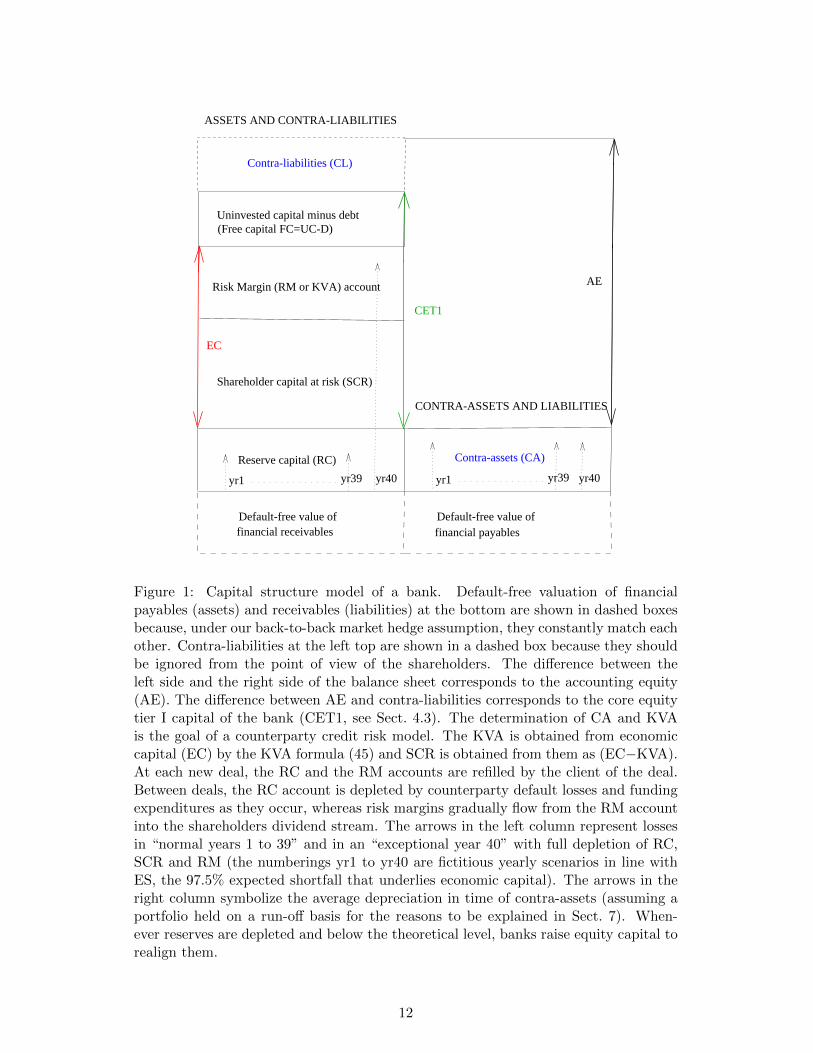
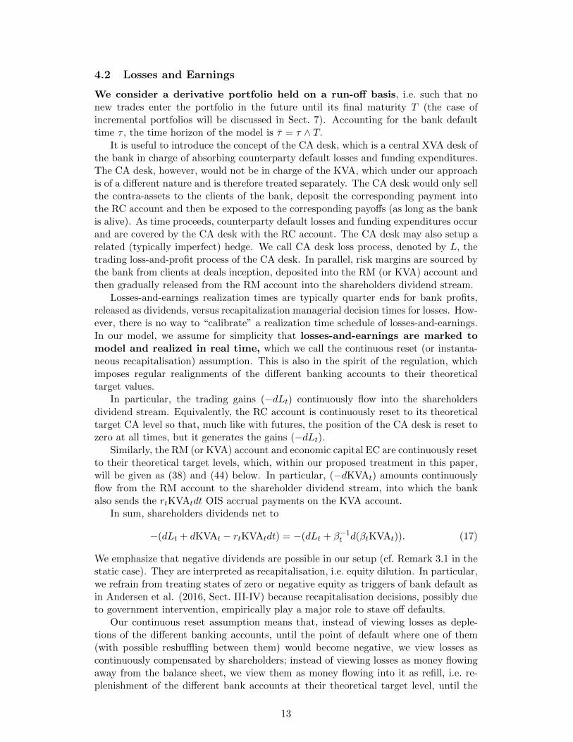
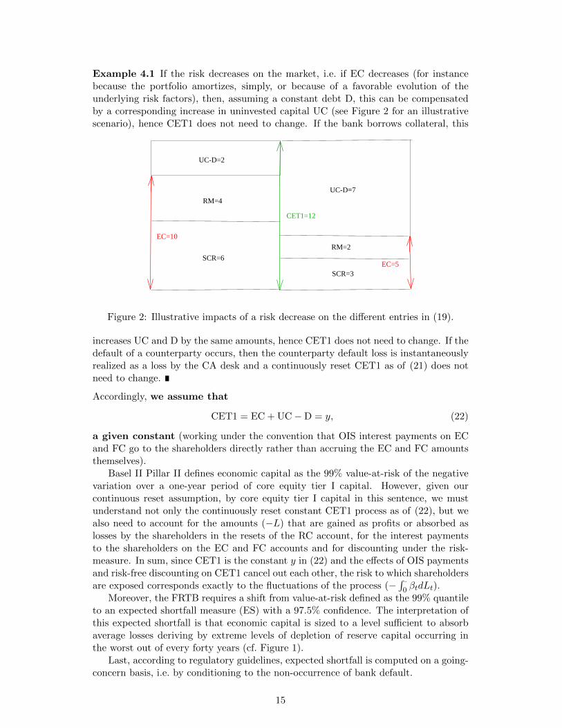
In Figure 1 we represent the difference FC=UC−D, the so called “free capital” ina Solvency II actuarial terminology, as a single line on the asset side.

11

Reserve capital (RC)

Shareholder capital at risk (SCR)

Risk Margin (RM or KVA) account

yr1

Uninvested capital minus debt

ASSETS AND CONTRA-LIABILITIES

CONTRA-ASSETS AND LIABILITIES

yr39 yr40

CET1

Default-free value of financial receivables

Default-free value offinancial payables

Contra-liabilities (CL)

yr1 yr39 yr40

Contra-assets (CA)

AE

(Free capital FC=UC-D)

EC

Figure 1: Capital structure model of a bank. Default-free valuation of financialpayables (assets) and receivables (liabilities) at the bottom are shown in dashed boxesbecause, under our back-to-back market hedge assumption, they constantly match eachother. Contra-liabilities at the left top are shown in a dashed box because they shouldbe ignored from the point of view of the shareholders. The difference between theleft side and the right side of the balance sheet corresponds to the accounting equity(AE). The difference between AE and contra-liabilities corresponds to the core equitytier I capital of the bank (CET1, see Sect. 4.3). The determination of CA and KVAis the goal of a counterparty credit risk model. The KVA is obtained from economiccapital (EC) by the KVA formula (45) and SCR is obtained from them as (EC−KVA).At each new deal, the RC and the RM accounts are refilled by the client of the deal.Between deals, the RC account is depleted by counterparty default losses and fundingexpenditures as they occur, whereas risk margins gradually flow from the RM accountinto the shareholders dividend stream. The arrows in the left column represent lossesin “normal years 1 to 39” and in an “exceptional year 40” with full depletion of RC,SCR and RM (the numberings yr1 to yr40 are fictitious yearly scenarios in line withES, the 97.5% expected shortfall that underlies economic capital). The arrows in theright column symbolize the average depreciation in time of contra-assets (assuming aportfolio held on a run-off basis for the reasons to be explained in Sect. 7). When-ever reserves are depleted and below the theoretical level, banks raise equity capital torealign them.

12

4.2 Losses and Earnings

We consider a derivative portfolio held on a run-off basis, i.e. such that nonew trades enter the portfolio in the future until its final maturity T (the case ofincremental portfolios will be discussed in Sect. 7). Accounting for the bank defaulttime τ , the time horizon of the model is τ = τ ∧ T.

It is useful to introduce the concept of the CA desk, which is a central XVA desk ofthe bank in charge of absorbing counterparty default losses and funding expenditures.The CA desk, however, would not be in charge of the KVA, which under our approachis of a different nature and is therefore treated separately. The CA desk would only sellthe contra-assets to the clients of the bank, deposit the corresponding payment intothe RC account and then be exposed to the corresponding payoffs (as long as the bankis alive). As time proceeds, counterparty default losses and funding expenditures occurand are covered by the CA desk with the RC account. The CA desk may also setup arelated (typically imperfect) hedge. We call CA desk loss process, denoted by L, thetrading loss-and-profit process of the CA desk. In parallel, risk margins are sourced bythe bank from clients at deals inception, deposited into the RM (or KVA) account andthen gradually released from the RM account into the shareholders dividend stream.

Losses-and-earnings realization times are typically quarter ends for bank profits,released as dividends, versus recapitalization managerial decision times for losses. How-ever, there is no way to “calibrate” a realization time schedule of losses-and-earnings.In our model, we assume for simplicity that losses-and-earnings are marked tomodel and realized in real time, which we call the continuous reset (or instanta-neous recapitalisation) assumption. This is also in the spirit of the regulation, whichimposes regular realignments of the different banking accounts to their theoreticaltarget values.

In particular, the trading gains (−dLt) continuously flow into the shareholdersdividend stream. Equivalently, the RC account is continuously reset to its theoreticaltarget CA level so that, much like with futures, the position of the CA desk is reset tozero at all times, but it generates the gains (−dLt).

Similarly, the RM (or KVA) account and economic capital EC are continuously resetto their theoretical target levels, which, within our proposed treatment in this paper,will be given as (38) and (44) below. In particular, (−dKVAt) amounts continuouslyflow from the RM account to the shareholder dividend stream, into which the bankalso sends the rtKVAtdt OIS accrual payments on the KVA account.

In sum, shareholders dividends net to

−(dLt + dKVAt − rtKVAtdt) = −(dLt + β−1t d(βtKVAt)). (17)

We emphasize that negative dividends are possible in our setup (cf. Remark 3.1 in thestatic case). They are interpreted as recapitalisation, i.e. equity dilution. In particular,we refrain from treating states of zero or negative equity as triggers of bank default asin Andersen et al. (2016, Sect. III-IV) because recapitalisation decisions, possibly dueto government intervention, empirically play a major role to stave off defaults.

Our continuous reset assumption means that, instead of viewing losses as deple-tions of the different banking accounts, until the point of default where one of them(with possible reshuffling between them) would become negative, we view losses ascontinuously compensated by shareholders; instead of viewing losses as money flowingaway from the balance sheet, we view them as money flowing into it as refill, i.e. re-plenishment of the different bank accounts at their theoretical target level, until the

13

point of default where the payers cease willing to do so. When this happens is modeledas a totally unpredictable event at some exogenous time calibrated to the bank CDSspread, which we view as the most reliable and informative credit data regarding antic-ipations of markets participants about future recapitalization, government interventionand other (including TLAC bail-in) bank failure resolution policies.

As demonstrated by the well-known difficulties in calibrating structural default timemodels, this view on the default time of the bank is actually more realistic and it isdefinitely more suitable for XVA analysis purposes, which requires a proper calibrationto the CDS curve of the bank.

Remark 4.1 In a Merton mindset, the default of the bank in our setup could bemodeled as the first time when UC goes below D, i.e. when the free capital FC=UC−Dbecomes negative (cf. Remark 3.1 in the one-period setup). Merton (1974)’s purposewas to develop an option-theoretic view on equity and corporate debt. For this ofcourse a structural model of the default time of a firm is required. In our case thereason why we introduce a capital structure model of the bank is not to come up withsuch a structural model of the bank default time, which for the above-explained reasonswould be unrealistic. Instead, the motivation for our capital structure model is to putthe contra-assets and contra-liabilities of a bank in a balance sheet perspective in orderto identify the structural connection between the different XVA metrics and show thatthe overall XVA problem is self-contained and well-posed. In particular, in the analysisof counterparty credit risk, the free capital process FC=UC−D has a very passive role.The key feature is the dividing line between contra-assets and contra-liabilities, itemswhich are not present in the Merton model.

4.3 Economic Capital

Core equity tier I capital (CET1) is the regulatory metric that represents the corefinancial strength of a bank. Since contra-liabilities do not benefit to the shareholders,CET1 is given by the difference between the overall result AE of the bank and CL, i.e.

CET1 = AE− CL = A− L− CA, (18)

by (16).Under our back-to-back market hedge assumption, default-free valuation of finan-

cial payables (assets) and receivables (liabilities) constantly match each other, so thatthe difference between assets and liabilities reduces to

A− L = RC + EC + FC (19)

(recalling EC=SCR+RM). Hence,

CET1 = A− L− CA

= (RC− CA) + (EC + FC).(20)

In the case of a back-to-back hedged portfolio held on a run-off basis with instantaneousrecapitalization, the first term is constantly reset to 0 (any discrepancy between RC andCA is instantaneously realized into (−dL)). Moreover, the impacts of the derivativeportfolio on the different entries in

CET1 = EC + FC = EC + UC−D (21)

are interconnected.

14

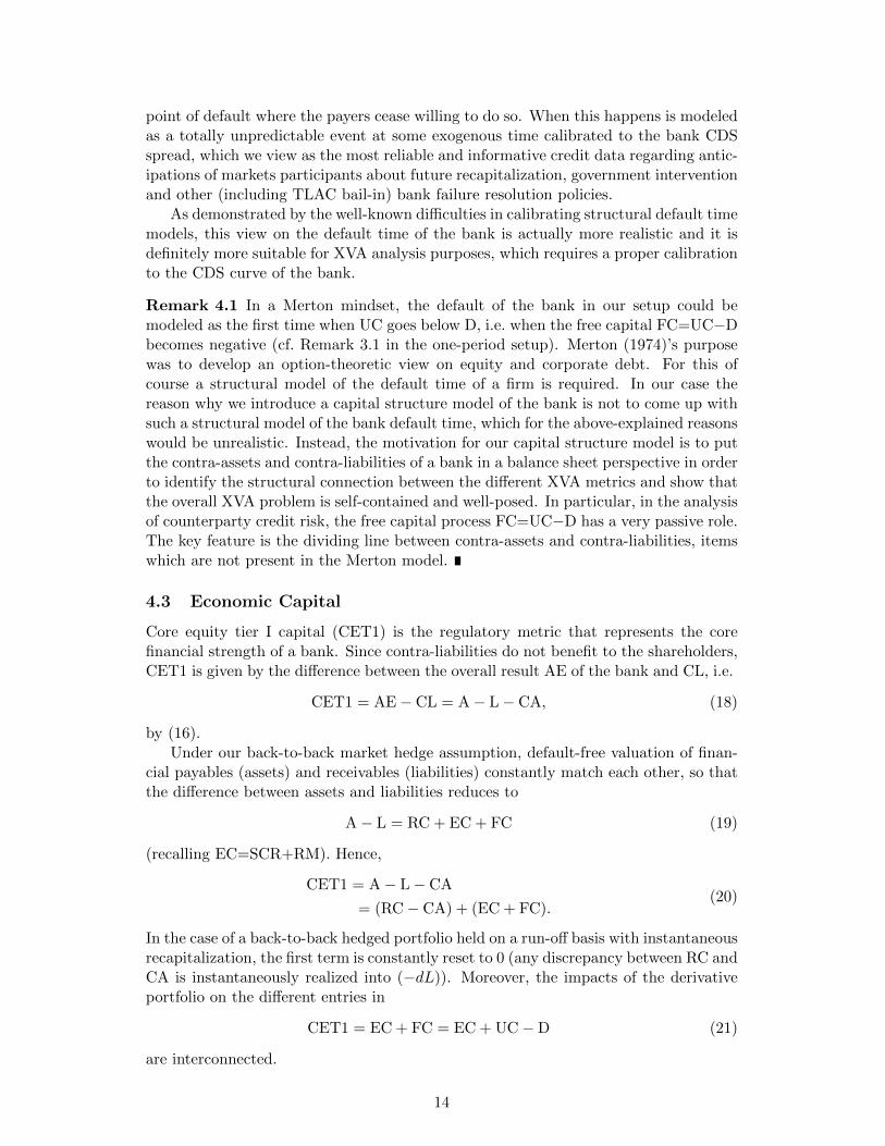
Example 4.1 If the risk decreases on the market, i.e. if EC decreases (for instancebecause the portfolio amortizes, simply, or because of a favorable evolution of theunderlying risk factors), then, assuming a constant debt D, this can be compensatedby a corresponding increase in uninvested capital UC (see Figure 2 for an illustrativescenario), hence CET1 does not need to change. If the bank borrows collateral, this

SCR=6

RM=4

UC-D=2

CET1=12

EC=10

SCR=3

RM=2

UC-D=7

EC=5

Figure 2: Illustrative impacts of a risk decrease on the different entries in (19).

increases UC and D by the same amounts, hence CET1 does not need to change. If thedefault of a counterparty occurs, then the counterparty default loss is instantaneouslyrealized as a loss by the CA desk and a continuously reset CET1 as of (21) does notneed to change.

Accordingly, we assume that

CET1 = EC + UC−D = y, (22)

a given constant (working under the convention that OIS interest payments on ECand FC go to the shareholders directly rather than accruing the EC and FC amountsthemselves).

Basel II Pillar II defines economic capital as the 99% value-at-risk of the negativevariation over a one-year period of core equity tier I capital. However, given ourcontinuous reset assumption, by core equity tier I capital in this sentence, we mustunderstand not only the continuously reset constant CET1 process as of (22), but wealso need to account for the amounts (−L) that are gained as profits or absorbed aslosses by the shareholders in the resets of the RC account, for the interest paymentsto the shareholders on the EC and FC accounts and for discounting under the risk-measure. In sum, since CET1 is the constant y in (22) and the effects of OIS paymentsand risk-free discounting on CET1 cancel out each other, the risk to which shareholdersare exposed corresponds exactly to the fluctuations of the process (−

∫ ·0 βtdLt).

Moreover, the FRTB requires a shift from value-at-risk defined as the 99% quantileto an expected shortfall measure (ES) with a 97.5% confidence. The interpretation ofthis expected shortfall is that economic capital is sized to a level sufficient to absorbaverage losses deriving by extreme levels of depletion of reserve capital occurring inthe worst out of every forty years (cf. Figure 1).

Last, according to regulatory guidelines, expected shortfall is computed on a going-concern basis, i.e. by conditioning to the non-occurrence of bank default.

15

In conclusion, our reference definition for economic capital is

ESt(L) =E[ ∫ t+1

t β−1t βsdLs1

∫ t+1t β−1

t βsdLs≥VaRt(L)∣∣Gt ∨ τ > t+ 1

]Q[ ∫ t+1

t β−1t βsdLs ≥ VaRt(L)

∣∣Gt ∨ τ > t+ 1] , (23)

where

VaRt(L) = inf` : Q

[ ∫ t+1

tβ−1t βsdLs > `

∣∣Gt ∨ τ > t+ 1]≤ 2.5%

.

Solvency II introduces a further modification as economic capital is required to bein excess of cost of capital (KVA in our setup). This modification is considered inSect. 6.2.

Note that, as it is only the fluctuations of L that matter in (23), the value of theunknown constant y in (22) is immaterial.

Summarizing key features of our setup:

Proposition 4.1 Assuming a back-to-back hedged portfolio held on a run-off basissatisfying (22) with continuous recapitalization until bank default:(i) Shareholder dividends are given by

−(dLt + dKVAt − rtKVAtdt) = −dLt − β−1t d(βtKVAt); (24)

(ii) The reference definition for economic capital is ES = ESt(L) as of (23).

Proof. This holds by construction in our setup (cf. the justifications for (17) and (23)given above).

The balance sheet perspective developed in this section has been key in identifyingthe economic meaning of the XVA accounting terms as well as the connections betweenthem. In particular, Proposition 4.1(ii) is telling us that the data required as input ineconomical capital and later in turn KVA computations correspond to the contra-assetsmis-hedge process L.

Thanks to this connection, the XVA problem as a whole is self-contained and, asit will therefore turn out in concrete setups (see e.g. Albanese, Caenazzo, and Crepey(2016)), well-posed. This is of course good news. But another good news is that, nowthat Proposition 4.1 has been established, in view of it, we can forget most of thecumbersome balance sheet data in the sequel of this paper and in any actual XVAmodeling, focusing on the key quantities CA, CL and on the process L, the latterplaying the role of a “dynamic reduced model” of the balance sheet.

5 Wealth Transfer Analysis

We denote by J = 1[0,τ) the survival indicator process of the bank. For any left-limited process Y, we denote by ∆τY = Yτ − Yτ− the jump of Y at τ and by Y τ− =JY + (1− J)Yτ− the process Y stopped before time τ , so that

dYt = dY τ−t + (−∆τY ) dJt, 0 ≤ t ≤ τ . (25)

16

We denote by C the cumulative stream of counterparty credit (as opposed to fund-ing or hedging) cash flows. Hence counterparty default losses contributing to CAcorrespond to Cτ−, whereas (−∆τC) contributes to CL.

The CA desk may setup a (partial) counterparty credit risk hedge. The hedgeis assumed to be funded separately from the derivative portfolio, being for instanceimplemented through repo markets or through assets with no upfront payment suchas CDS contracts. The hedging gain process of the CA desk, including the cost ofsetting the hedge, is modeled as Hτ−, for some risk neutral local martingale H startingfrom 0. The rationale here is that hedging gains arise in practice as the stochasticintegral of predictable hedging ratios against (funding cost inclusive) wealth processesof individual hedging assets. Under our standing valuation rule, each hedging asset isvalued as risk-free discounted expectation of its future cash flows. Hence, the individualwealth process related to a long position in any of the hedging assets is a risk-neutrallocal martingale, as is in turn the stochastic integral H. However, it is only the Hτ−component of H that contributes to CA, whereas (−∆τH) contributes to CL.

Example 5.1 In the Black-Scholes model with constant interest rate r on a stock Swith volatility σ, assuming that the hedge is implemented through a repo market withzero repo basis on S, then (assuming no dividends on S)

dHt = ζt(dS − rStdt

)= ζtσStdWt, (26)

where W is the risk-neutral Brownian motion driving S and ζ is the hedging ratio inS. The instantaneous cost of funding the hedge is ζtrStdt, which is included in (26).

Likewise, the funding expenditures of the CA desk are modeled as

−rtCAtdt+ dFτ−, (27)

for some risk neutral local martingale F starting from 0. Here the rationale is thatfunding is implemented in practice as the stochastic integral of predictable hedgingratios against funding assets. Given our standing valuation rule, the value process ofeach of these assets is a martingale modulo risk-free accrual. Therefore the fundingcosts generated by the funding strategy of the CA desk accumulate into a local mar-tingale F stopped before τ , i.e. Fτ−, minus the risk-free accrual of the value CA thatsits on the reserve capital account (under our continuous reset assumption). The cashflow (−∆τF) contributes to CL.

Example 5.2 Let

dBt = rtBtdt

dDt = (rt + λt)Dtdt+ (1−R)Dt−dJt = rtDtdt+Dt−(λtdt+ (1−R) dJt

)represent the risk-free OIS deposit asset and a risky bond issued by the bank for itsinvesting and unsecured borrowing purposes. Here λ represents an unsecured fundingspread and R is some recovery coefficient, taken as an exogenous constant (as thepositive impact of trades on the realized recovery of the bank is not reflected in thebank funding spreads, cf. Sect. 2.1.1). The risk-neutral martingale condition thatapplies to (βD) under our standing valuation framework implies that λ = (1 − R)γ,where γ is the risk-neutral default intensity of the bank, so that

λtdt+ (1−R) dJt = (1−R)dµt,

17

where dµt = γdt + dJt is the compensated jump-to-default martingale of the bank.We assume a dynamic amount of collateral Ct on the derivative portfolio, borrowedunsecured and posted by the bank if Ct > 0, received and invested at OIS rate by thebank if Ct < 0, remunerated OIS by the receiving party to the posting party. Thecorresponding funding policy of the bank is represented by a splitting of the amountCAt on the RC account (under our continuously reset convention) as

CAt =(Ct + (CAt − Ct)+

)︸ ︷︷ ︸Invested at the risk-free rate as νtBt

− (CAt − Ct)−︸ ︷︷ ︸Unsecurely funded as ηtDt

.(28)

A standard self-financing condition expressing the conservation of cash flows at thelevel of the bank as a whole yields

d (νtBt − ηtDt) = νtdBt − ηt−dDt

= νtrtBtdt− ηt(rt + λt)Dtdt− (1−R)ητ−Dτ−dJt

= rtCAtdt− (1−R)ηt−Dt−dµt, 0 ≤ t ≤ τ

(a left-limit in time is required in η because D jumps at time τ, so that the process η,which is defined implicitly through (CA−−C) in (28), is not predictable). Equivalentlyviewed in terms of costs, i.e. flipping signs in the above, we obtain

− d (νtBt − ηtDt) = −rtCAtdt+ dFt = (−rtCAtdt+ dFτ−t ) + (−∆τF) dJt,

where we set dFt = (1−R)(CAt− − Ct−)−dµt.

Lemma 5.1 Assuming a back-to-back hedged portfolio held on a run-off basis satisfy-ing (22) with continuous recapitalization until the bank default time τ , given the credit,funding and hedging cash flows stream C,F and H :(i) Assuming integrability, we have, for 0 ≤ t ≤ τ ,

CAt = Et∫ τ

tβ−1t βsdCτ−s + Et

∫ τ

tβ−1t βsdFτ−s + Et[β−1

t βτ1τ<T∆τH]

CLt = Et[β−1t βτ1τ<T(−∆τC −∆τF + ∆τH)

]CCRt = Et

∫ τ

tβ−1t βsdCs.

(29)

(ii) The CA desk loss process L is given as the risk-neutral local martingale such that

βtdLt = d(βtCAt) + βt(dCτ−t + dFτ−t − dHτ−t ), 0 ≤ t ≤ τ , (30)

starting from the accrued loss L0 = z of the CA desk.

Proof. (i) In view of (27), the funding expenditures in excess over risk-free accrual atrate r of reserve capital, i.e. in excess over a cost (−rtCAtdt) (typically negative cost,i.e. benefit), appear as Fτ−. Hence, accounting for Remark 2.1 as far as the valuationof the funding cash flows in CA is concerned, by definition, we have

CAt = Et∫ τ

tβ−1t βs(dCτ−s + dFτ−s − dHτ−s )

CLt = Et[β−1t βτ1τ<T(−∆τC −∆τF + ∆τH)

]CCRt = CAt − CLt = Et

∫ τ

tβ−1t βs(dCs + dFs − dHs),

(31)

18

from which (29) is deduced by the martingale properties of F and H.(ii) The different cash flows contributing to the CA desk loss process L are the coun-terparty default losses prior to time τ, which correspond to dCτ−, and the fundingexpenditures given by (27), minus the CA hedging gains dHτ−. Also accounting forthe mark-to-model of the liabilities, valued by the CA process, of the CA desk, theloss-and-profit process L appears as

dLt = dCAt + dCτ−t − rtCAtdt+ dFτ−t − dHτ−t ,

which is equivalent to (30), where the right-hand side is a local martingale in view ofthe first identity in (29).

Remark 5.1 Note that, assuming integrability, the CA risk-neutral valuation formulain (29) is equivalent to a martingale condition on L joint with a terminal conditionCAτ = 0 (cf. the comments following (9) in the static setup). This underlies anotherpoint of view on valuation, where no valuation opertor is introduced, but L is insteadassumed to be a risk-neutral local martingale, jointly with a terminal condition CAτ =0. Under these alternative assumptions the ensuing CA formulas would be the same. Amartingale condition on L can be interpreted as a shareholder no-arbitrage condition.

The following immediate corollary to Lemma 5.1 shows that contra-liabilities canbe interpreted as a wealth transfer triggered by deals away from shareholders, due tothe impossibility for the bank to hedge its own jump-to-default risk.

Theorem 5.1 The formula CCRt = Et∫ τt β−1t βsdCs holds independently of the fund-

ing and hedging policy of the bank. Moreover:(i) If the bank could replicate its own default, i.e. for ∆τH = ∆τC + ∆τF , then wewould have

CL = 0, CA = CCR. (32)

(ii) But the bank cannot hedge its own default, i.e. ∆τH = 0, hence

CAt = Et∫ τ

tβ−1t βsdCτ−s + Et

∫ τ

tβ−1t βsdFτ−s ,

CLt = Et[β−1t βτ1τ<T(−∆τC)

]+ Et

[β−1t βτ1τ<T(−∆τF)

].

(33)

In the special case where

dHt = β−1t d(βtCAt) + dCτ−t + dFτ−t , 0 ≤ t ≤ τ (34)

(assuming this would be an achievable hedging gain process), then the process L isconstant and (23) yields ES = 0.

The default exposure of the derivative portfolio as well as the collateralization andfunding policies of the bank determine the data C and F of the CA, CL and L processes.Once C and F are specified, Theorem 5.1 can be turned into concrete formulas for allthe XVA components and for the dynamics of the process L which is required as inputdata in KVA computations. See Albanese et al. (2016) for illustration in the case of abank engaged into bilateral portolios. Note that the process F typically involves theCA process, hence the CA formula in (33) is in fact an equation for the CA process(cf. the developments following (8) in a static setup and see Example 5.2).

19

The industry terminology tends to distinguish an FVA in the technical sense of thecost of funding cash collateral for variation margin from an MVA defined as the cost offunding segregated collateral posted as initial margin (see Albanese et al. (2016)). Theacademic literature tends to merge the two in an overall FVA meant in the broadersense of the cost of funding the derivative trading strategy of the bank. Such an overallFVA would correspond to the second term in the CA formula in (33), where the firstterm corresponds to the CVA (cf. the static CA formula (8)). The first and secondterms in the CL formula in (33) correspond to the continuous-time analogs of the DVAand FDA in the static CL formula (12).

5.1 Connection with the Modigliani and Miller (1958) Theorem

The Modigliani and Miller (1958) theorem includes two key assumptions. One is that,as a consequence of trading, total wealth is conserved. The second assumption is thatmarkets are complete. In our setup we keep the wealth conservation hypothesis butwe lift the completeness. This ensures the validity of the part of the theorem statingthat the wealth of the bank as a whole should not depend on the funding policy of thebank, which corresponds to the first statement in Theorem 5.1. But the part statingthat the interests of shareholders and creditors are aligned with each other, i.e. that(32) holds, is only valid if the bank can hedge its own default. Since this is not thecase in practice, the derivative portfolio of the bank triggers a wealth transfer from theshareholders to the creditors by the amount CL in (33).

Besides, the impossibility of replicating counterparty default losses (the hedginggain process in (34) is typically not achievable in practice) implies that the process Lis not constant but fluctuates in time. Hence, capital needs to be set at risk by theshareholders, which therefore deserve a risk premium. This risk premium is graduallyreleased to shareholders in the form of the RM (or KVA) payments, which is the topicof the next section.

Remark 5.2 The situation of market incompleteness that we consider in this paperis that of a bank subject to trading constraints preventing it from hedging jump-to-default risk. For different (unrelated to counteparty credit risk) extensions of theModigliani and Miller (1958) theorem in incomplete markets, see Gottardi (1995) andthe references there.

6 Cost of Capital

To generate a dividend flow as a risk compensation to the bank shareholders, the bankclients are asked to pay an additional amount, which in the insurance literature iscalled risk margin, while in the banking literature it is currently called capital valuationadjustment (KVA). The KVA is not treated as reserve capital, but rather as a retainedearning which contributes to economic capital and is different from CA in that it is nota capital deduction. The level of compensation required by shareholders is driven bymarket considerations. Typically, investors in banks expect a hurdle rate h of about10% to 12%. In this paper we work with an exogenous and constant hurdle rate h. Anendogenous h would arise in a situation of competitive equilibrium between differentbanks (as opposed to our setup where only one bank is considered).

When a bank charges cost of capital to clients, these revenues are accounted foras profits. However, since prevailing accounting standards for derivative securities are

20

based on the theoretical assumption of market completeness, they do not envision amechanism to retain these earnings for the purpose of remunerating capital across theentire life of transactions that can be as long as decades. In complete markets, there isno justification for market and credit risk capital (the only justification for reservingcapital is to cover operational risk, which we do not consider in this paper). Hence,mark-to-market profits are immediately distributable. A strategy of earning retentionbeyond the end of the ongoing accounting year (or quarter) is still possible as in allfirms, but this would be regarded as purely a business decision, not subject to financialregulation under the Basel III Accord.

This leads to an explosive instability characteristic of a leverage ratchet effect. Forinstance, if a bank starts off today by entering a 30-year swap with a client, the bankbooks a profit. Assuming the trade is perfectly hedged, the profit is distributable atonce. The following year, the bank still needs capital to absorb the risk of the 29-yearswap in the portfolio. In order to remunerate shareholders, given that the profits fromthis trade have already been distributed the previous year, the bank has no other optionthan to lever up, i.e. sell and hedge another swap, book a new profit and distributethe dividend to shareholders that are now posting capital for both swaps. As longas trading volumes grow exponentially, the scheme self-sustains. When exponentialgrowth stops, the bank return on equity crashes. The financial crisis of 2007-2008 canbe largely explained along these lines (see Figure 3). In the aftermath of the crisis,the first casualty was the return on equity for the fixed income business as profitshad already been distributed and market-level hurdle rates could not be sustained byportfolio growth.

Figure 3: Global financial crisis Ponzi scheme (Source: Office of the comptroller of thecurrency, Q3 2015 quarterly bank trading revenue report).

Interestingly enough, however, in the insurance domain, the Swiss Solvency Test(2004) and Solvency II, unlike Basel III, do regulate the distribution of retained earn-

21

ings through a mechanism tied to so called risk margins envisioned as cost of capital.Also, the accounting standards set out in IFRS 4 Phase II (see IFRS (2012, 2013)are consistent with Solvency II and include a treatment for risk margins that has noanalogue in the banking domain. See Wuthrich and Merz (2013), Eisele and Artzner(2011) and Salzmann and Wuthrich (2010) regarding the risk margin and cost of capitalactuarial literature.

The purpose of this section is to discuss a Solvency II inspired framework for as-sessing cost of capital (KVA) for a bank, pass it on to the bank clients and distributeit gradually to the bank shareholders through a dividend policy which would be sus-tainable even in the limit case of a portfolio held on a run-off basis, with no new tradesever entered in the future.

Solvency II requires in addition that EC must be higher than the ensuing riskmargin (i.e. the KVA). In this paper, we show how to handle this constraint and howto handle it optimally.

Remark 6.1 The purpose of this article is to discuss general principles and, from thisviewpoint, it seems clear that Solvency II establishes a strong precedent which onecannot ignore. Even under the current banking regulatory environment, it would beperfectly possible for the board of directors of a bank to decide to implement the KVAstrategy of this paper on a voluntary basis, even without a prescriptive regulatoryenvironment, as a way to implement a sustainable dividend distribution policy.

6.1 KVA Equations

Let C ≥ ES represent a putative economic capital process for the bank. To size theKVA we ask the following question: What should be the level K = Kt(C) of a KVAaccount ending up with Kτ = 0 and such that the ensuing dividend stream

−(dLt + dKVAt − rtKVAtdt) (35)

(cf. (24)) corresponds to an average (expected) remuneration h(Ct − Kt)dt at eachpoint in time t ∈ [0, τ ] to the shareholders?

The reason why Kτ = 0 is because less would mean insufficient and more would bewasteful. More precisely, if the KVA was negative at any point in time before τ , thiswould mean that the RM account was insufficiently provisioned to satisfy shareholdersremuneration requirement for their capital at risk. A jump to a negative value at theexact time τ in case τ < T might not be an issue. Such a scenario looks a bit artificialanyway. We exclude it for the sake of the well-posedness of the KVA equation. As wewill prove in Theorem 6.1(ii), proceeding along the above lines yields a KVA processwhich is nonnegative on [0, τ ], as desired.

The reason why (Ct−Kt) appears rather than Ct after (35) is because risk marginsare loss-absorbing and therefore part of the economic capital. Therefore, shareholdercapital at risk, which by assumption is remunerated at the hurdle rate h, only corre-sponds to the difference (Ct −Kt).

The above-sketched approach can be contrasted with alternative KVA approachesin the literature, developed by Green, Kenyon, and Dennis (2014) and Green andKenyon (2016) or Elouerkhaoui (2016), where all the pricing adjustments are viewedas part of fair valuation and where, in particular, the KVA is treated as a contra-assetfor reserve capital such as CVA or FVA, as if the KVA was a capital deduction. Bycontrast, we consider that, as risk margin is retained earnings meant to be released to

22

the bank shareholders, it does not belong to the balance sheet as a liability. This viewis consistent with the treatment of the risk margin in Swiss solvency test capital atrisk calculations.

Under our standing modelling assumptions, we have P = Q, under which the CAdesk loss process L is a local martingale. Hence the above conditions on the processK reduce to

Kτ = 0 and dKt +(h(Ct −Kt)− rtKt

)dt is a local martingale on [0, τ ]. (36)

This differential specification is in the form of a linear backward stochastic differ-ential equation (BSDE, see El Karoui, Hamadene, and Matoussi (2009) for a survey),equivalent to the integrated form (37) below. As we demonstrate in Lemma 6.1 below,the solution K = Kt(C) to this equation is unique. Furthermore, since the equationis linear, the solution is given by the explicit formula (39). However, the difference(Ct −Kt) represents shareholder capital at risk and must therefore be nonnegative. Ifone accounts for the resulting consistency condition C ≥ K(C), then, as we will see indetail in Sect. 6.2, the KVA BSDE becomes of Lipschitz type (38), which, as our nextresult shows, is also well-posed.

We denote by Lp the space of ·p-integrable processes over [0, τ ], for any p ≥ 1.

Lemma 6.1 Consider the following BSDEs:

Kt = Et∫ τ

t

(hCs − (rs + h)Ks

)ds, t ∈ [0, τ ], (37)

KVAt = Et∫ τ

t

(hmax(ESs,KVAs)− (rs + h)KVAs

)ds, t ∈ [0, τ ] (38)

to be solved for respective processes K and KVA. Assuming that r is bounded from belowand that C (respectively ES) and r are in L2, then the BSDE (37) (respectively (38))is well posed in L2, where well-posedness includes existence, uniqueness, and so-calledcomparison.

The L2 solution K to (37) admits the explicit representation

Kt = hEt∫ τ

te−

∫ st (ru+h)duCsds, t ∈ [0, τ ]. (39)

In case the process L is constant, then ES and the solution KVA to (38) vanish.

Proof. In terms of the coefficient

ft(k) = h(

max(ESt, k)− k)− rtk = hmax

(ESt, k

)− (rt + h)k, k ∈ R, (40)

the KVA BSDE (38) appears as

KVAt = Et∫ τ

tfs(KVAs)ds, t ∈ [0, τ ]. (41)

For any real k, k′ ∈ R and t ∈ [0, τ ], we have(ft(k)− ft(k′)

)(k − k′) = −(rt + h)(k − k′)2 + h

(max(ESt, k)−max(ESt, k

′))(k − k′))

≤ −rt(k − k′)2 ≤ C(k − k′)2,

23

for some constant C (having assumed r bounded from below), so that the coefficientf satisfies the so-called monotonicity condition. Moreover, for |k| ≤ k, we have:

|f·(k)− f·(0)| ≤ hmax(|ES|, k

)+ |h+ r|k + hES+.

Hence, assuming that ES and r are in L2, the following integrability conditions hold:

sup|k|≤k

|f·(k)− f·(0)| ∈ L1, for any k > 0, and f·(0) ∈ L2.

Therefore, by application of the general filtration BSDE results of Kruse and Popier(2016, Sect. 5), the BSDE (41) is well-posed in L2, where well-posedness includesexistence, uniqueness and comparison. Even simpler computations prove the analogousstatements regarding the linear BSDE (37). Moreover, (39) obviously solves (37).Finally, in case L is constant, then ES vanishes and KVA = 0 obviously solves (38).

6.2 The KVA Constrained Optimization Problem

Under the Solvency II capital requirement, economic capital is the sum between share-holder capital at risk (SCR) and risk margin (the insurance analog of the KVA, whichare also loss-absorbing). Some actuarial literature dwells with the puzzle according towhich the calculation of the risk margin depends on economic capital projections in thefuture, while economic capital itself depends on the risk margin, an apparently circulardependency (see e.g. Salzmann and Wuthrich (2010, Sect. 4.4) and Robert (2013)).

This paper addresses the problem of circular dependency as follows. First wecompute the economic capital according to some risk measure. Then we define KVAusing economic capital projections discounted at a hurdle rate as of (39). Our SCR isdefined a posteriori as the difference (EC−KVA).

However, for so doing, we need to account for the additional constraint that EC ≥KVA. Otherwise this would break the consistency condition

SCR ≥ 0. (42)

Remark 6.2 In our notation, the Solvency II accounting condition in Wuthrich andMerz (2013, Definition 9.15 (a)) reads SCR ≥ CA − RC. In our continuously resetframework where CA = RC at all times, this condition is the same as (42).

A BSDE based KVA approach allows addressing the constraint (42) as follows. Toemphasize the dependence of K on C, we henceforth denote by K(C) the solution (39)to the linear BSDE (37). We define the set of admissible economic capital processes

C = C ∈ L2;C ≥ max(ES,K(C)

), (43)

where C ≥ ES is the risk acceptability condition and C ≥ K(C) is the consistenycondition (cf. the respective conditions (b) and (a) and their discussion in Wuthrichand Merz (2013, pages 270 and 271)). Assuming ES in L2, we define

EC = max(ES,KVA), (44)

where KVA is the L2 solution to the BSDE (38).

24

Lemma 6.2 Assuming that r is bounded from below and that ES and r are in L2,the solution KVA to (38) solves the linear BSDE (37) for the implicit data C = EC,i.e. we have KVA = K(EC), that is,

KVAt = hEt∫ τ

te−

∫ st (ru+h)duECsds, t ∈ [0, τ ]. (45)

In particular, the KVA process discounted at the OIS rate is a supermartingale.

Proof. The process KVA is in L2 and, by virtue of (38) and (44), we have, for t ∈ [0, τ ],

KVAt = Et∫ τ

t

(hmax

(ESs,KVAs

)− (rs + h)KVAs

)ds

= Et∫ τ

t

(hECs − (rs + h)KVAs

)ds.

(46)

Hence, the process KVA solves the linear BSDE (37) for C = EC ∈ L2. The identityKVA = K(EC) follows by uniqueness of an L2 solution to the linear BSDE (37)established in Lemma 6.1. Equation (45) follows by an application of (39). Thesupermartingale property of the KVA discounted at the OIS rate is visible in thefollowing differential form of (46): KVAτ = 0 and

dKVAt +(h(ECt −KVAt)− rtKVAt

)dt is a local martingale on [0, τ ], (47)

i.e.

d(βKVA)t + hβt(ECt −KVAt)dt is a local martingale on [0, τ ], (48)

where the drift is nonnegative by definition (44) of EC.

The next result shows that the consistency condition SCR ≥ 0 is optimally handled bydefining the KVA through the BSDE (38) and the ensuing EC process as (44). In fact,EC thus defined is the minimal admissible economic capital process, with the cheapestensuing cost of capital given by the KVA, which is also shown to be nondecreasing inthe hurdle rate h.

Theorem 6.1 Under the assumptions of Lemma 6.2, we have:(i) EC = min C,KVA = minC∈CK(C);(ii) The process KVA is nonnegative and it is nondecreasing in h.

Proof. (i) We saw in Lemma 6.2 that KVA = K(EC), hence

EC = max(ES,KVA) = max(ES,K(EC)

),

therefore EC ∈ C. Moreover, for any C ∈ C, we have (cf. (40)):

ft(Kt(C)) = hmax(ESt,Kt(C)

)− (rt + h)Kt(C) ≤ hCt − (h+ rt)Kt(C).

Hence, the coefficient f of the KVA BSDE (38) never exceeds the coefficient of the linearBSDE (37) when both coefficients are evaluated at the solution Kt(C) of (37). Sincethese are BSDEs with equal (null) terminal condition, the BSDE comparison theoremapplied to the BSDEs (37) and (38) (see Kruse and Popier (2016, Proposition 4 and

25

Remark 3)) yields KVA ≤ K(C). Consequently, KVA = minC∈CK(C) and, for anyC ∈ C,

C ≥ max(ES,K(C)) ≥ max(ES,KVA) = EC.

Hence EC = min C.(ii) The 97.5% expected shortfall of a centered random variable is nonnegative. HenceES is nonnegative and the KVA is nonnegative, by (45) and (44). Since ES is nonneg-ative, then, as visible in (40), the coefficient ft(k) of the KVA BSDE (38) is nonde-creasing in the hurdle rate parameter h. So is therefore in turn the L2 solution KVAto (38), by the BSDE comparison theorem of Kruse and Popier (2016, Proposition 4and Remark 3) applied to the BSDE (38) for different values of h.

7 Incremental XVA Methodology

In all the above the derivative portfolio of the bank is assumed held on a run-off basis,i.e. set up at time 0 and assuming that no new trades will ever enter the portfolio inthe future until its final maturity T . In practice derivative portfolios are incrementaland models are precisely required for computing incremental XVA values at everynew trade. This last section of the paper relates the run-off assumption to a pricingapproach myopic to the trade-flow, as this cannot be anticipated by a market maker,and which would be sustainable even in the limit case where no new trades wouldbe entered into the future. This way, we arrive to a sustainable strategy for profitretention, which is the key principle behind Solvency II.

Banks are market makers and, as such, they are price makers. Bank clients areprice takers willing to accept a loss in a trade for the sake of receiving benefits thatbecome apparent only once one includes their real investment portfolio, which cannotbe done explicitly in a pricing model.

The manager of a market maker portfolio cannot decide on asset selection: tradesare proposed by clients and the market maker needs to stand ready to bid for a trade ata suitable price no matter what the trade is and when it arrives. A new trade has twoimpacts: it triggers a wealth transfer from shareholders to bondholders and alters therisk profile of the portfolio. This is reflected by a jump of the balance sheet, from theone related to the endowment (pre-trade portfolio) right before the time t = 0 (say) thenew deal is considered, to the one related to the portfolio including the new deal. Letus denote by “∆·” the corresponding jump of any of our balance sheet metrics in Figure1. Again, the arrival process for new trades and the client decision whether to acceptthe bank bid or not follow stochastic processes which cannot be anticipated. Thereforethe corresponding jumps in the balance sheet cannot be predicted or offset ex-ante.Once a trade happens, it has to be computed at the moment and, for upgrading fromone balance sheet to the other at the new deal, a market maker has no other optionthan asking clients to refill the RC and RM accounts by the required amounts of

∆RC = ∆CA and ∆RM = ∆KVA, (49)

where the equalities hold by virtue of the continuous reset assumption in each of thebalance sheets.

If future trades could be anticipated (this is the argument in Hull and White(2016)), then one could optimise further and assess the fair valuation of debt aheadof time to compensate for the anticipated occurrence of wealth transfers. This wouldlead to greater efficiencies and allow banks to bid for trades at entry prices given by

26

unadjusted fair valuations. However, the impossibility of anticipating new trades andotherwise offsetting wealth transfers, justifies the use of incremental XVAs computedunder the run-off assumption in the balance sheets with and without the new deal.

In view of (49) and (1), consistent with the preliminary static setup formulas (15),the all-inclusive XVA add-on to the entry price for a new deal, dubbed funds transferprice (FTP), appears as

FTP = ∆CA + ∆KVA = ∆CCR + ∆CL + ∆KVA, (50)

where ∆CCR would be the counterparty credit risk add-on fair to the bank as awhole, ∆CL is the compensation for the wealth triggered by the new deal away fromshareholders and ∆KVA is their premium for the risk on their equity arising from themis-hedge of the contra-assets (mis-hedge of counterparty default losses and fundingexpenditures), all computed in an incremental run-off basis as explained above.

Obviously, the endowment has a key impact on the FTP of a new trade. It may verywell happen that a new deal is risk-reducing with respect to the pre-existing portfolio,in which case FTP < 0.

8 Conclusion

To conclude this paper we emphasize its main technical insights.In order to focus on counterparty credit risk and XVAs, we assume that the market

risk of the bank is perfectly hedged by means of perfectly collateralized back-to-backtrades. This back-to-back hedge perspective does not only result in more concisederivation of the XVA equations, direct as opposed to two-step in most other XVAreferences in the literature, where XVA equations are obtained as the difference betweena linear equation for the mark-to-market of the portfolio ignoring counterparty creditrisk and another equation for the “risky value” of the portfolio. The back-to-backhedge perspective also yields a much clearer view on the cash flows that generate thecontra-liabilities. In particular, Section 3 clarifies in an elementary static setup how,accounting for the back-to-back hedge, these cash flows are not a fiction or an abstractcompensation of others, but actual cash flows that fall into the estate of the defaultedbank and increase the realized recovery rate of creditors.

We root our XVA approach on a capital structure model, depicted in Figure 1 inSection 4.2, acknowledging the impossibility for a bank to replicate jump-to-defaultrelated cash flows. Such a balance sheet perspective is key in identifying the eco-nomic meaning of the XVA accounting terms as well as the connections between them.As synthetized in Proposition 4.1 and Theorem 5.1, due to counterparty credit riskincompleteness, the derivative portfolio of the bank triggers a wealth transfer fromshareholders to creditors that can only be compensated by a corresponding add-on toentry prices.

Moreover, shareholders bear the trading risk of a central XVA desk (dubbed CAdesk in this paper) in charge of counterparty risk and funding within the bank. OurKVA is formalized as the cost (45) of a remuneration policy of shareholder capital atrisk, which would be sustainable even in the limit case of a portfolio held on a run-off basis, with no new trades ever entered in the future. Conceived in the spirit of aportfolio optimization tool for a derivative market maker in incomplete counterpartycredit risk markets, the KVA in this sense is a risk premium tuned in order to keepthe shareholders on an “efficient frontier” such that

27

“Average instantaneous returnt = Risk aversion h × Risk measuret × dt”(cf. (36)). Our KVA definition is genuinely dynamic, as opposed to multi-period simplyin the Solvency II actuarial literature. This allows us to solve the puzzle according towhich the calculation of the risk margin depends on economic capital projections in thefuture while economic capital itself depends on the risk margin, an apparently circulardependency. Specifically, Theorem 6.1 states and solves the ensuing KVA problem as aconstrained optimization problem, where economic capital and its cost are minimizedunder a nonnegativity consistency condition on the ensuing shareholder capital at risk(SCR, which in our model appears endogenously as the difference between economiccapital and the KVA).

Under the structural approach of this paper, the KVA is a risk premium takingas input data the contra-assets mis-hedge loss-and-profit process L. Thanks to thisconnection, the CA equation for contra-assets valuation and the KVA equation, i.e. theXVA equations as a whole, are a self-contained problem.

As opposed to the other XVAs, our KVA is not the valuation of some cash flows,but a risk premium. As risk margin is retained earnings meant to be released to thebank shareholders, the KVA in our sense does not belong to the balance sheet as aliability, at least not statically as part of contra-assets. But, in some sense, the KVAis a measure of the fluctuations of the balance sheet.

A last important output of this work is that the ensuing XVA methodology, eventhough rooted in the analysis of a bank balance sheet, does not require problematicbalance sheet data. All it requires in practice is the modeling of the trading loss-and-profit process L, which plays the role of a reduced dynamic model of the balance sheet.We refer the reader to Albanese, Caenazzo, and Crepey (2016) for illustration in theconcrete setup of a bank engaged in bilateral trade portfolios.

A Assumptions

We list the key assumptions by order of appearance in the body of the paper, withcomments. At the bottom of this work lies the fact that a bank cannot replicate jump-to-default exposures. However we do not state this as a standing assumption, becauseit is instructive to see what would happen if a bank could replicate jump-to-defaultexposures (we then find that CL=KVA=0).

A key assumption is (A5), as it also underlies (A6) through (A9).

(A1) All cash flows are valued by their risk-free discounted (G,Q) conditionalexpectation, assumed to exist.

Ensures the internal consistency of the valuation setup.

(A2) Derivative entry prices include, on top of the valuation of the corre-sponding cash flows, a KVA risk premium.

Remunerates bank shareholders for their capital at risk that needs be reservedagainst trading risk (mis-hedge of contra-assets, under (A4)).

(A3) The historical probability measure P coincides with the pricing mea-sure Q.

As little of relevance can be said about the historical probability measure forXVA computations entailing projections over decades, the discrepancy betweenP and Q is left to model risk.

28

(A4) The market risk of the bank is perfectly hedged by means of perfectlycollateralized back-to-back trades.

Made in order to focus on counterparty credit risk and XVAs. Yields directderivations of the XVA equations. Harmless as far as the equations themselvesare concerned.

(A5) A bank is a market maker which cannot anticipate future trades.

Implies that banks do have trading costs and have no other option than passingthese costs to their clients to survive in the long run.

(A6) The positive impact of trades on the realized recovery of the bank isnot reflected in the bank funding spreads.

A consequence of (A5). The positive impact of future trades on the realizedrecovery of the bank is not anticipated and therefore not reflected in the price ofborrowing for funding these trades.

(A7) We consider a derivative portfolio held on a run-off basis.

The right assumption to make, incrementally at every new trade, in order toachieve pricing and dividend policies that are robust, i.e. sustainable even in thelimit case where no new trades would ever be entered in the future (cf. (A5)).

(A8) Losses-and-earnings are marked to model and realized in real time.

Until the payers cease willing to do so and the bank defaults. This is in the spiritof the regulation which imposes regular realignments of the different bankingaccounts to their theoretical target values.

(A9) CET1 = EC + UC−D = y, a given constant.

A natural complement of the run-off and continuous reset assumptions (A7) and(A8).

B Acronyms

A Assets.

AE Accounting equity.

BSDE Backward stochastic differential equation.

CA Contra-assets (or their valuation).

CCR Counterparty credit risk (or its valuation).

CL Contra-liabilities (or their valuation).

CDS Credit default swap.

CET1 Core equity tier I capital.

CVA Credit valuation adjustment.

D Debt.

29

DVA Debt valuation adjustment.

EC Economic capital.

ES Expected shortfall.

FC Free capital (UC−D).

FDA Funding debt adjustment (the contra-liability counterpart of the FVA).

FRTB Fundamental review of the trading book.

FTP Funds transfer price.

FVA Funding valuation adjustment.

IFRS International financial reporting standards.

KVA Capital valuation adjustment (the banking notion of risk margin).

L Liabilities.

OIS Overnight index swap.

RC Reserve capital (or CA account).

RM Risk margins (or KVA) account.

SCR Shareholder capital at risk.

TLAC Total loss-absorbing capacity.

UC Uninvested capital.

XVA Generic “X” valuation adjustment

References

Albanese, C. and L. Andersen (2014). Accounting for OTC derivatives: Fundingadjustments and the re-hypothecation option. ssrn:2482955.

Albanese, C., L. Andersen, and S. Iabichino (2015). FVA: Accounting and risk man-agement. Risk Magazine, February 64–68.

Albanese, C., S. Caenazzo, and S. Crepey (2016). Funding, margin and capitalvaluation adjustments for bilateral trade portfolios. Working paper available athttps://math.maths.univ-evry.fr/crepey.

Andersen, L., D. Duffie, and Y. Song (2016). Funding value adjustments.ssrn.2746010.

BCBS (2013). Consultative document: Fundamental Review of the Trading Book: Arevised market risk framework. Basel Committee on Bank Supervision, October.http://www.bis.org/publ/bcbs265.pdf.

Capponi, A. and S. Crepey (2016). Endogenous KVA. In preparation.

Cochrane, J. and J. Saa-Requejo (2000). Beyond arbitrage: “Good deal” asset pricebounds in incomplete markets. Journal of Political Economy 108 (1), 79–119.

30

Duffie, D. and M. Huang (1996). Swap rates and credit quality. Journal of Fi-nance 51, 921–950.

Eisele, K.-T. and P. Artzner (2011). Multiperiod insurance supervision: top-downmodels. European Actuarial Journal 1 (1), 107–130.

El Karoui, N., S. Hamadene, and A. Matoussi (2009). Backward stochastic differen-tial equations and applications. In Indifference Pricing: Theory and Applications,Chapter 8, pp. 267–320. Princeton University Press.

Elouerkhaoui, Y. (2016). From FVA to KVA: including cost of capital in derivativespricing. Risk Magazine, March 70–75.

Gottardi, P. (1995). An analysis of the conditions for the validity of Modigliani-MillerTheorem with incomplete markets. Economic Theory 5, 191–207.

Green, A. and C. Kenyon (2016). Accounting for KVA under IFRS 13. Risk Maga-zine, March 64–68. Long version available as ssrn.620454.

Green, A., C. Kenyon, and C. Dennis (2014). KVA: capital valuation adjustment byreplication. Risk Magazine, December. Preprint version available under the title“KVA: capital valuation adjustment” as ssrn.620454.

Hull, J. and A. White (2016). XVAs: A gap between theory and practice. RiskMagazine, April 50–52.

IFRS (2012). IFRS 13 fair value measurement. IFRS .http://www.iasplus.com/en/news/2011/May/news6909.

IFRS (2013). IFRS 4 insurance contracts exposure draft. IFRS .http://www.ifrs.org/Current-Projects/IASB-Projects/Insurance-Contracts/Exposure-Draft-June-2013/Documents/ED-Insurance-Contracts-June-2013.pdf.

Kruse, T. and A. Popier (2016). BSDEs with monotone generator driven by Brow-nian and Poisson noises in a general filtration. Stochastics: An InternationalJournal of Probability and Stochastic Processes 88 (4), 491–539.

Madan, D. (2015). Asset pricing theory for two price economies. Annals of Fi-nance 11 (1), 1–35.

Merton, R. (1974). On the pricing of corporate debt: the risk structure of interestrates. The Journal of Finance 29, 449–470.

Modigliani, F. and M. Miller (1958). The cost of capital, corporation finance andthe theory of investment. Economic Review 48, 261–297.

Myers, S. (1977). Determinants of corporate borrowing. Journal of Financial Eco-nomics 5, 147–175.

Robert, C. (2013). Market value margin calculations under the cost of capital ap-proach within a bayesian chain ladder framework. Insurance: Mathematics andEconomics 53, 216–229.

Rogers, L. C. G. (2001). Duality in constrained optimal investment and consumptionproblems: a synthesis. Lecture notes.

Salzmann, R. and M. Wuthrich (2010). Cost-of-capital margin for a general insuranceliability runoff. ASTIN Bulletin 40 (2), 415–451.

31

Schweizer, M. (2001). A guided tour through quadratic hedging approaches. In J. C.E. Jouini and M. Musiela (Eds.), Option Pricing, Interest Rates and Risk Man-agement, Volume 12, pp. 538–574. Cambridge University Press.

Swiss Solvency Test (2004). The risk margin for the Swiss solvency test. Swiss FederalOffice for Private Insurance, September 17.

Wuthrich, M. and M. Merz (2013). Financial Modeling, Actuarial Valuation andSolvency in Insurance. Springer.

32