xtableGallery-2

The xtable gallery

Jonathan Swinton <[email protected]>with small contributions from others

September 12, 2014

1 Summary

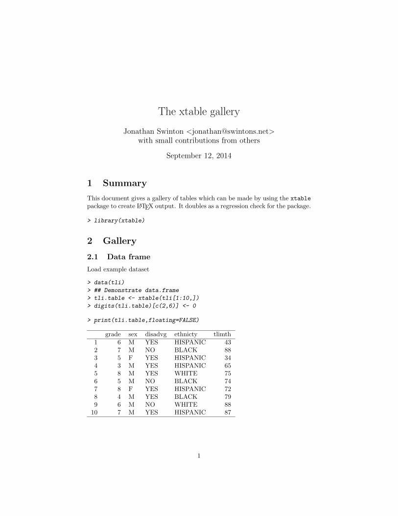
This document gives a gallery of tables which can be made by using the xtable

package to create LATEX output. It doubles as a regression check for the package.

> library(xtable)

2 Gallery

2.1 Data frame

Load example dataset

> data(tli)

> ## Demonstrate data.frame

> tli.table <- xtable(tli[1:10,])

> digits(tli.table)[c(2,6)] <- 0

> print(tli.table,floating=FALSE)

grade sex disadvg ethnicty tlimth1 6 M YES HISPANIC 432 7 M NO BLACK 883 5 F YES HISPANIC 344 3 M YES HISPANIC 655 8 M YES WHITE 756 5 M NO BLACK 747 8 F YES HISPANIC 728 4 M YES BLACK 799 6 M NO WHITE 88

10 7 M YES HISPANIC 87

1

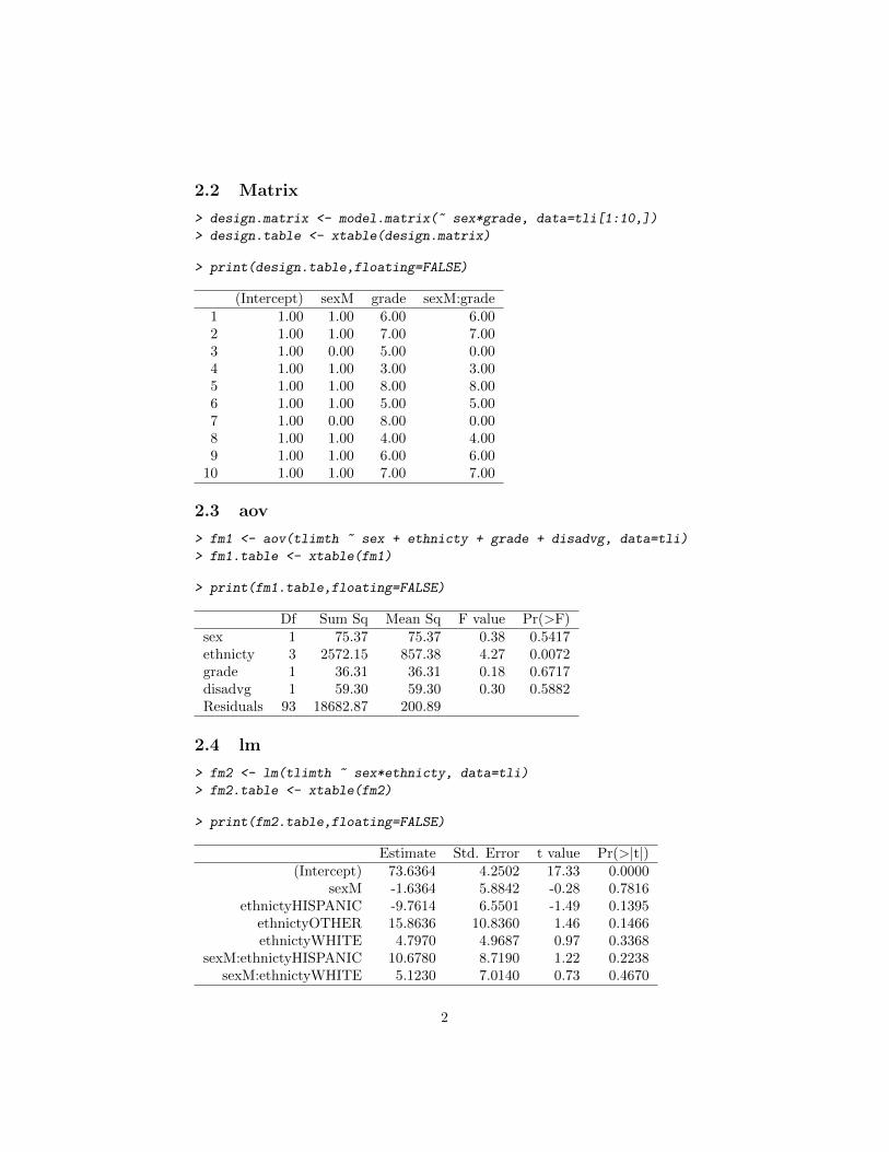
2.2 Matrix

> design.matrix <- model.matrix(~ sex*grade, data=tli[1:10,])

> design.table <- xtable(design.matrix)

> print(design.table,floating=FALSE)

(Intercept) sexM grade sexM:grade1 1.00 1.00 6.00 6.002 1.00 1.00 7.00 7.003 1.00 0.00 5.00 0.004 1.00 1.00 3.00 3.005 1.00 1.00 8.00 8.006 1.00 1.00 5.00 5.007 1.00 0.00 8.00 0.008 1.00 1.00 4.00 4.009 1.00 1.00 6.00 6.00

10 1.00 1.00 7.00 7.00

2.3 aov

> fm1 <- aov(tlimth ~ sex + ethnicty + grade + disadvg, data=tli)

> fm1.table <- xtable(fm1)

> print(fm1.table,floating=FALSE)

Df Sum Sq Mean Sq F value Pr(>F)sex 1 75.37 75.37 0.38 0.5417ethnicty 3 2572.15 857.38 4.27 0.0072grade 1 36.31 36.31 0.18 0.6717disadvg 1 59.30 59.30 0.30 0.5882Residuals 93 18682.87 200.89

2.4 lm

> fm2 <- lm(tlimth ~ sex*ethnicty, data=tli)



Estimate Std. Error t value Pr(>|t|)(Intercept) 73.6364 4.2502 17.33 0.0000

sexM -1.6364 5.8842 -0.28 0.7816ethnictyHISPANIC -9.7614 6.5501 -1.49 0.1395

ethnictyOTHER 15.8636 10.8360 1.46 0.1466ethnictyWHITE 4.7970 4.9687 0.97 0.3368

sexM:ethnictyHISPANIC 10.6780 8.7190 1.22 0.2238sexM:ethnictyWHITE 5.1230 7.0140 0.73 0.4670

2

2.4.1 anova object

> print(xtable(anova(fm2)),floating=FALSE)

Df Sum Sq Mean Sq F value Pr(>F)sex 1 75.37 75.37 0.38 0.5395ethnicty 3 2572.15 857.38 4.31 0.0068sex:ethnicty 2 298.43 149.22 0.75 0.4748Residuals 93 18480.04 198.71

2.4.2 Another anova object

> fm2b <- lm(tlimth ~ ethnicty, data=tli)

> print(xtable(anova(fm2b,fm2)),floating=FALSE)

Res.Df RSS Df Sum of Sq F Pr(>F)1 96 19053.592 93 18480.04 3 573.55 0.96 0.4141

2.5 glm

> ## Demonstrate glm

> fm3 <- glm(disadvg ~ ethnicty*grade, data=tli, family=binomial())



Estimate Std. Error z value Pr(>|z|)(Intercept) 3.1888 1.5966 2.00 0.0458

ethnictyHISPANIC -0.2848 2.4808 -0.11 0.9086ethnictyOTHER 212.1701 22122.7093 0.01 0.9923ethnictyWHITE -8.8150 3.3355 -2.64 0.0082

grade -0.5308 0.2892 -1.84 0.0665ethnictyHISPANIC:grade 0.2448 0.4357 0.56 0.5742

ethnictyOTHER:grade -32.6014 3393.4687 -0.01 0.9923ethnictyWHITE:grade 1.0171 0.5185 1.96 0.0498

2.5.1 anova object

> print(xtable(anova(fm3)),floating=FALSE)

Df Deviance Resid. Df Resid. DevNULL 99 129.49ethnicty 3 47.24 96 82.25grade 1 1.73 95 80.52ethnicty:grade 3 7.20 92 73.32

3

2.6 More aov

> ## Demonstrate aov

> ## Taken from help(aov) in R 1.1.1

> ## From Venables and Ripley (1997) p.210.

> N <- c(0,1,0,1,1,1,0,0,0,1,1,0,1,1,0,0,1,0,1,0,1,1,0,0)

> P <- c(1,1,0,0,0,1,0,1,1,1,0,0,0,1,0,1,1,0,0,1,0,1,1,0)

> K <- c(1,0,0,1,0,1,1,0,0,1,0,1,0,1,1,0,0,0,1,1,1,0,1,0)

> yield <- c(49.5,62.8,46.8,57.0,59.8,58.5,55.5,56.0,62.8,55.8,69.5,55.0,

+ 62.0,48.8,45.5,44.2,52.0,51.5,49.8,48.8,57.2,59.0,53.2,56.0)

> npk <- data.frame(block=gl(6,4), N=factor(N), P=factor(P), K=factor(K), yield=yield)

> npk.aov <- aov(yield ~ block + N*P*K, npk)

> op <- options(contrasts=c("contr.helmert", "contr.treatment"))

> npk.aovE <- aov(yield ~ N*P*K + Error(block), npk)

> options(op)

> #summary(npk.aov)

> print(xtable(npk.aov),floating=FALSE)

Df Sum Sq Mean Sq F value Pr(>F)block 5 343.30 68.66 4.45 0.0159N 1 189.28 189.28 12.26 0.0044P 1 8.40 8.40 0.54 0.4749K 1 95.20 95.20 6.17 0.0288N:P 1 21.28 21.28 1.38 0.2632N:K 1 33.13 33.13 2.15 0.1686P:K 1 0.48 0.48 0.03 0.8628Residuals 12 185.29 15.44

2.6.1 anova object

> print(xtable(anova(npk.aov)),floating=FALSE)


2.6.2 Another anova object

> print(xtable(summary(npk.aov)),floating=FALSE)

4


> #summary(npk.aovE)

> print(xtable(npk.aovE),floating=FALSE)

Df Sum Sq Mean Sq F value Pr(>F)N:P:K 1 37.00 37.00 0.48 0.5252Residuals 4 306.29 76.57N 1 189.28 189.28 12.26 0.0044P 1 8.40 8.40 0.54 0.4749K 1 95.20 95.20 6.17 0.0288N:P 1 21.28 21.28 1.38 0.2632N:K 1 33.14 33.14 2.15 0.1686P:K 1 0.48 0.48 0.03 0.8628Residuals1 12 185.29 15.44

> print(xtable(summary(npk.aovE)),floating=FALSE)

Df Sum Sq Mean Sq F value Pr(>F)N:P:K 1 37.00 37.00 0.48 0.5252Residuals 4 306.29 76.57N 1 189.28 189.28 12.26 0.0044P 1 8.40 8.40 0.54 0.4749K 1 95.20 95.20 6.17 0.0288N:P 1 21.28 21.28 1.38 0.2632N:K 1 33.14 33.14 2.15 0.1686P:K 1 0.48 0.48 0.03 0.8628Residuals1 12 185.29 15.44

2.7 More lm

> ## Demonstrate lm

> ## Taken from help(lm) in R 1.1.1

> ## Annette Dobson (1990) "An Introduction to Generalized Linear Models".

> ## Page 9: Plant Weight Data.

> ctl <- c(4.17,5.58,5.18,6.11,4.50,4.61,5.17,4.53,5.33,5.14)

> trt <- c(4.81,4.17,4.41,3.59,5.87,3.83,6.03,4.89,4.32,4.69)

> group <- gl(2,10,20, labels=c("Ctl","Trt"))

5

> weight <- c(ctl, trt)

> lm.D9 <- lm(weight ~ group)

> print(xtable(lm.D9),floating=FALSE)


groupTrt -0.3710 0.3114 -1.19 0.2490

> print(xtable(anova(lm.D9)),floating=FALSE)

Df Sum Sq Mean Sq F value Pr(>F)group 1 0.69 0.69 1.42 0.2490Residuals 18 8.73 0.48

2.8 More glm

> ## Demonstrate glm

> ## Taken from help(glm) in R 1.1.1

> ## Annette Dobson (1990) "An Introduction to Generalized Linear Models".

> ## Page 93: Randomized Controlled Trial :

> counts <- c(18,17,15,20,10,20,25,13,12)

> outcome <- gl(3,1,9)

> treatment <- gl(3,3)

> d.AD <- data.frame(treatment, outcome, counts)

> glm.D93 <- glm(counts ~ outcome + treatment, family=poisson())

> print(xtable(glm.D93,align="r|llrc"),floating=FALSE)

Estimate Std. Error z value Pr(>|z|)(Intercept) 3.0445 0.1709 17.81 0.0000outcome2 -0.4543 0.2022 -2.25 0.0246outcome3 -0.2930 0.1927 -1.52 0.1285

treatment2 0.0000 0.2000 0.00 1.0000treatment3 0.0000 0.2000 0.00 1.0000

2.9 prcomp

> if(require(stats,quietly=TRUE)) {

+ ## Demonstrate prcomp

+ ## Taken from help(prcomp) in mva package of R 1.1.1

+ data(USArrests)

+ pr1 <- prcomp(USArrests)

+ }

> if(require(stats,quietly=TRUE)) {

+ print(xtable(pr1),floating=FALSE)

+ }

6

PC1 PC2 PC3 PC4Murder 0.0417 -0.0448 0.0799 -0.9949Assault 0.9952 -0.0588 -0.0676 0.0389

UrbanPop 0.0463 0.9769 -0.2005 -0.0582Rape 0.0752 0.2007 0.9741 0.0723

> print(xtable(summary(pr1)),floating=FALSE)

PC1 PC2 PC3 PC4Standard deviation 83.7324 14.2124 6.4894 2.4828

Proportion of Variance 0.9655 0.0278 0.0058 0.0008Cumulative Proportion 0.9655 0.9933 0.9991 1.0000

> # ## Demonstrate princomp

> # ## Taken from help(princomp) in mva package of R 1.1.1

> # pr2 <- princomp(USArrests)

> # print(xtable(pr2))

2.10 Time series

> temp.ts <- ts(cumsum(1+round(rnorm(100), 0)), start = c(1954, 7), frequency=12)

> temp.table <- xtable(temp.ts,digits=0)

> caption(temp.table) <- "Time series example"

> print(temp.table,floating=FALSE)

Jan Feb Mar Apr May Jun Jul Aug Sep Oct Nov Dec1954 1 0 -1 -1 -1 01955 2 4 6 7 8 9 10 12 13 13 12 151956 15 16 18 20 21 20 21 21 21 24 26 271957 30 32 32 34 36 36 37 37 40 39 40 391958 40 39 40 42 42 45 45 46 49 51 53 561959 57 60 61 60 62 64 64 66 69 68 70 701960 71 72 75 75 75 76 78 79 79 80 80 811961 82 83 84 86 86 87 87 87 88 89 92 911962 92 93 92 92 92 92 94 98 99 99

3 Sanitization

> insane <- data.frame(Name=c("Ampersand","Greater than","Less than","Underscore","Per cent","Dollar","Backslash","Hash", "Caret", "Tilde","Left brace","Right brace"),

+ Character = I(c("&",">", "<", "_", "%", "$", "\\", "#", "^", "~","{","}")))

> colnames(insane)[2] <- paste(insane[,2],collapse="")

> print( xtable(insane))

Sometimes you might want to have your own sanitization function

> wanttex <- xtable(data.frame( label=paste("Value_is $10^{-",1:3,"}$",sep="")))

> print(wanttex,sanitize.text.function=function(str)gsub("_","\\_",str,fixed=TRUE))

7

Name &>< %$\#^˜{}1 Ampersand &2 Greater than >3 Less than <4 Underscore5 Per cent %6 Dollar $7 Backslash \8 Hash #9 Caret ^

10 Tilde ˜11 Left brace {12 Right brace }

label1 Value is 10−1

2 Value is 10−2

3 Value is 10−3

3.1 Markup in tables

Markup can be kept in tables, including column and row names, by using acustom sanitize.text.function:

> mat <- round(matrix(c(0.9, 0.89, 200, 0.045, 2.0), c(1, 5)), 4)

> rownames(mat) <- "$y_{t-1}$"

> colnames(mat) <- c("$R^2$", "$\\bar{R}^2$", "F-stat", "S.E.E", "DW")

> mat <- xtable(mat)

> print(mat, sanitize.text.function = function(x){x})

R2 R̄2 F-stat S.E.E DWyt−1 0.90 0.89 200.00 0.04 2.00

You can also have sanitize functions that are specific to column or row names.In the table below, the row name is not sanitized but column names and tableelements are:

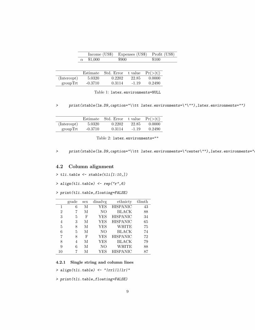
> money <- matrix(c("$1,000","$900","$100"),ncol=3,dimnames=list("$\\alpha$",c("Income (US$)","Expenses (US$)","Profit (US$)")))

> print(xtable(money),sanitize.rownames.function=function(x) {x})

4 Format examples

4.1 Adding a centering environment

> print(xtable(lm.D9,caption="\\tt latex.environments=NULL"),latex.environments=NULL)

8

Income (US$) Expenses (US$) Profit (US$)α $1,000 $900 $100


groupTrt -0.3710 0.3114 -1.19 0.2490

Table 1: latex.environments=NULL

> print(xtable(lm.D9,caption="\\tt latex.environments=\"\""),latex.environments="")


groupTrt -0.3710 0.3114 -1.19 0.2490

Table 2: latex.environments=""

> print(xtable(lm.D9,caption="\\tt latex.environments=\"center\""),latex.environments="center")

4.2 Column alignment

> tli.table <- xtable(tli[1:10,])

> align(tli.table) <- rep("r",6)




4.2.1 Single string and column lines

> align(tli.table) <- "|rrl|l|lr|"


9


groupTrt -0.3710 0.3114 -1.19 0.2490

Table 3: latex.environments="center"



4.2.2 Fixed width columns

> align(tli.table) <- "|rr|lp{3cm}l|r|"




4.3 Significant digits

Specify with a single argument

> digits(tli.table) <- 3

> print(tli.table,floating=FALSE,)

10


10 7 M YES HISPANIC 87or one for each column, counting the row names

> digits(tli.table) <- 1:(ncol(tli)+1)



10 7 M YES HISPANIC 87or as a full matrix

> digits(tli.table) <- matrix( 0:4, nrow = 10, ncol = ncol(tli)+1 )




11

4.4 Suppress row names

> print((tli.table),include.rownames=FALSE,floating=FALSE)

grade sex disadvg ethnicty tlimth6 M YES HISPANIC 437 M NO BLACK 885 F YES HISPANIC 343 M YES HISPANIC 658 M YES WHITE 755 M NO BLACK 748 F YES HISPANIC 724 M YES BLACK 796 M NO WHITE 887 M YES HISPANIC 87

If you want a vertical line on the left, you need to change the align attribute.

> align(tli.table) <- "|r|r|lp{3cm}l|r|"

> print((tli.table),include.rownames=FALSE,floating=FALSE)

grade sex disadvg ethnicty tlimth6 M YES HISPANIC 437 M NO BLACK 885 F YES HISPANIC 343 M YES HISPANIC 658 M YES WHITE 755 M NO BLACK 748 F YES HISPANIC 724 M YES BLACK 796 M NO WHITE 887 M YES HISPANIC 87

Revert the alignment to what is was before.

> align(tli.table) <- "|rr|lp{3cm}l|r|"

4.5 Suppress column names

> print((tli.table),include.colnames=FALSE,floating=FALSE)

12

1 6 M YES HISPANIC 432 7 M NO BLACK 883 5 F YES HISPANIC 344 3 M YES HISPANIC 655 8 M YES WHITE 756 5 M NO BLACK 747 8 F YES HISPANIC 728 4 M YES BLACK 799 6 M NO WHITE 88

10 7 M YES HISPANIC 87Note the doubled header lines which can be suppressed with, eg,

> print(tli.table,include.colnames=FALSE,floating=FALSE,hline.after=c(0,nrow(tli.table)))



4.6 Suppress row and column names

> print((tli.table),include.colnames=FALSE,include.rownames=FALSE,floating=FALSE)

6 M YES HISPANIC 437 M NO BLACK 885 F YES HISPANIC 343 M YES HISPANIC 658 M YES WHITE 755 M NO BLACK 748 F YES HISPANIC 724 M YES BLACK 796 M NO WHITE 887 M YES HISPANIC 87

4.7 Rotate row and column names

The rotate.rownames and rotate.colnames arguments can be used to rotatethe row and/or column names.

> print((tli.table),rotate.rownames=TRUE,rotate.colnames=TRUE)

13

gra

de

sex

dis

ad

vg

ethnic

ty

tlim

th


2 7 M NO BLACK 88

3 5 F YES HISPANIC 344 3 M YES HISPANIC 65

5 8 M YES WHITE 75

6 5 M NO BLACK 74

7 8 F YES HISPANIC 72

8 4 M YES BLACK 79

9 6 M NO WHITE 88


4.8 Horizontal lines

4.8.1 Line locations

Use the hline.after argument to specify the position of the horizontal lines.

> print(xtable(anova(glm.D93)),hline.after=c(1),floating=FALSE)

Df Deviance Resid. Df Resid. DevNULL 8 10.58outcome 2 5.45 6 5.13treatment 2 0.00 4 5.13

4.8.2 Line styles

The LATEXpackage booktabs can be used to specify different line style tagsfor top, middle, and bottom lines. Specifying booktabs = TRUE will lead toseparate tags being generated for the three line types.

Insert \usepackage{booktabs} in your LATEXpreamble and define the toprule,midrule, and bottomrule tags to specify the line styles. By default, whenno value is given for hline.after, a toprule will be drawn above the ta-ble, a midrule after the table headings and a bottomrule below the table.The width of the top and bottom rules can be set by supplying a value to\heavyrulewidth. The width of the midrules can be set by supplying a valueto \lightrulewidth. The following tables have \heavyrulewidth = 2pt and\lightrulewidth = 0.5pt, to ensure the difference in weight is noticeable.

There is no support for \cmidrule or \specialrule although they are partof the booktabs package.

> print(tli.table, booktabs=TRUE, floating = FALSE)

14

grade sex disadvg ethnicty tlimth



If hline.after includes −1, a toprule will be drawn above the table.If hline.after includes the number of rows in the table, a bottomrule willbe drawn below the table. For any other values specified in hline.after, amidrule will be drawn after that line of the table.

The next table has more than one midrule.

> bktbs <- xtable(matrix(1:10, ncol = 2))

> hlines <- c(-1,0,1,nrow(bktbs))

This command produces the required table.

> print(bktbs, booktabs = TRUE, hline.after = hlines, floating = FALSE)

1 2

1 1 6

2 2 73 3 84 4 95 5 10

4.9 Table-level LATEX

> print(xtable(anova(glm.D93)),size="small",floating=FALSE)

Df Deviance Resid. Df Resid. Dev

NULL 8 10.58outcome 2 5.45 6 5.13treatment 2 0.00 4 5.13

4.10 Long tables

Remember to insert \usepackage{longtable} in your LATEXpreamble.

15

> ## Demonstration of longtable support.

> x <- matrix(rnorm(1000), ncol = 10)

> x.big <- xtable(x,label='tabbig',

+ caption='Example of longtable spanning several pages')

> print(x.big,tabular.environment='longtable',floating=FALSE)

1 2 3 4 5 6 7 8 9 101 0.85 -0.33 0.13 1.27 -0.60 0.98 -0.50 0.12 -1.57 0.642 0.72 0.03 0.67 1.73 2.38 -1.19 0.22 -3.50 -1.73 -0.253 0.74 -0.26 -0.98 1.24 0.33 -1.37 -0.39 0.08 0.28 -0.404 2.06 -0.55 -0.64 0.56 0.50 -1.83 -0.08 -0.98 0.28 -0.185 0.89 -1.91 0.21 -0.46 0.06 -0.24 -0.70 -0.14 0.40 -0.996 -0.13 -1.06 -1.65 0.45 -0.36 0.15 0.48 0.49 -2.32 0.917 0.90 -0.70 0.96 -1.38 -0.82 -0.14 0.19 -0.88 -0.89 -0.598 -1.07 -0.13 -0.98 1.27 2.14 0.15 -0.31 1.09 -1.02 -0.199 -0.68 1.09 1.35 -0.35 2.36 0.41 -1.38 -1.08 -0.31 0.41

10 0.42 1.35 -0.43 0.35 -0.25 -0.99 -0.70 0.65 -0.55 -0.1511 -0.12 0.07 -1.01 -0.67 0.93 1.10 0.43 -1.57 -0.02 -0.0312 -0.77 0.42 -0.29 0.72 0.36 -2.49 1.89 0.11 0.89 -0.8413 1.54 -0.09 -0.31 0.66 -1.45 1.02 -1.00 0.05 0.54 1.2214 1.33 1.30 -1.23 -0.48 -0.23 0.57 0.29 0.20 -0.61 2.0515 -0.27 -1.63 0.55 -0.37 -0.15 1.02 1.43 0.19 -0.89 0.5316 0.10 0.48 -2.35 0.23 0.40 -0.53 0.51 0.49 1.33 -2.2117 0.49 0.40 -0.89 -0.21 -1.06 1.55 0.93 -0.28 -0.25 1.1218 -1.22 1.03 -2.01 -0.51 -0.32 -0.73 -1.42 -0.48 0.47 0.4619 1.18 -3.20 2.04 -1.04 -0.46 0.38 -1.07 1.21 -0.28 -0.2920 -0.18 -0.84 -1.24 -1.17 -0.88 1.61 -0.66 0.31 0.87 0.0621 -0.30 0.35 -1.39 0.32 -0.24 -0.91 0.71 -0.93 0.96 1.3122 1.36 0.16 -1.44 0.02 -0.23 -0.25 1.27 1.58 -1.54 -1.4223 2.06 0.52 1.44 -1.55 0.20 0.25 -1.07 -0.34 -0.72 -0.7924 0.94 -0.84 -0.37 -0.37 -0.83 3.50 1.10 -0.51 1.47 1.1025 -0.49 -0.63 -1.05 0.20 1.31 -1.45 0.57 -0.63 -1.05 0.4326 -0.41 -1.40 -0.35 0.12 -0.38 1.45 -0.32 -0.19 0.38 0.0727 0.27 0.67 -0.93 1.06 -0.41 0.26 -0.46 1.33 0.53 0.5028 0.96 -0.85 0.31 -0.75 0.07 0.04 -0.10 1.42 0.14 2.2429 1.20 -1.42 -0.86 -0.84 0.18 0.58 0.18 -0.63 0.07 1.0230 -0.19 -0.62 -0.60 -0.29 -0.53 -0.79 0.13 -1.54 0.22 0.8631 -0.01 0.11 0.89 -1.02 -0.20 1.87 1.37 -0.10 -0.42 -0.0532 0.93 1.96 0.55 0.01 2.11 0.27 -1.30 2.75 -0.04 0.4733 -0.10 0.21 -0.28 0.33 2.21 -1.25 0.42 1.20 0.53 0.9334 -1.22 0.25 1.24 -1.74 1.64 -0.70 -0.12 -0.70 -0.46 -0.8135 -0.40 1.29 0.04 1.14 0.21 -0.75 -2.25 -1.49 1.04 -0.9236 -0.60 -0.44 -2.34 0.18 -0.03 0.10 0.07 0.13 0.60 -0.0837 1.43 0.50 -1.79 -0.23 1.11 1.03 1.14 1.07 0.59 -0.60

16

38 1.26 0.36 -0.32 0.35 0.79 -0.37 -0.02 0.66 0.57 1.0439 0.04 0.57 -1.03 -1.42 1.92 1.85 1.31 -2.60 1.32 0.6440 0.60 0.14 -0.09 0.69 1.03 0.94 -0.28 -0.50 0.68 -0.8241 -1.13 -1.38 2.43 -0.44 0.04 1.32 0.29 -1.56 1.63 -0.7842 -1.07 -1.86 -0.69 -1.02 -0.81 1.03 1.11 -0.83 0.30 0.2843 0.30 -1.86 0.63 -0.10 -0.11 0.85 -0.67 -0.04 -0.26 0.4044 -1.79 -0.40 -0.83 0.10 -0.48 0.69 0.17 1.50 0.81 -0.3445 1.28 -0.35 0.16 -1.51 -0.45 -1.06 -0.96 -1.24 -1.55 -0.8346 0.59 0.07 -0.80 0.63 -0.23 1.36 -0.07 -0.88 0.36 -0.2047 2.21 -1.42 0.94 -0.92 -0.78 -1.17 0.68 0.48 -0.84 -0.3648 2.85 1.98 -0.49 -0.27 -0.73 -0.08 0.21 0.00 1.26 -1.1149 1.49 0.58 2.64 -1.31 -1.10 0.37 -1.08 1.84 -0.29 0.7450 1.07 0.23 0.87 0.67 0.86 0.51 -1.28 -0.82 0.64 2.6451 0.29 0.14 -0.64 -1.07 0.55 1.74 1.48 -1.41 1.10 -0.3252 0.27 -2.34 0.27 1.87 0.80 0.07 -1.13 0.93 0.72 2.7953 -1.75 1.59 0.67 -0.09 -0.47 -0.44 0.35 1.32 0.27 2.4154 0.28 1.41 -1.79 0.50 0.67 1.61 0.28 -0.25 0.60 0.0355 -1.01 -0.74 -1.36 -0.85 -0.36 0.35 0.40 -0.20 0.91 0.8956 -0.09 -0.21 -0.48 0.76 0.17 -1.55 1.26 2.54 -0.31 -0.4657 1.33 1.12 0.27 -0.91 0.35 0.32 -0.21 -0.23 -1.77 -0.1558 2.09 0.10 1.83 -0.41 1.09 -0.57 -0.83 0.29 0.65 0.6459 0.53 0.56 -0.83 0.37 0.04 0.28 0.46 -1.44 0.36 -0.8460 -0.24 -0.05 1.31 1.18 0.66 -0.28 -0.18 -2.50 0.87 1.1761 2.08 -0.62 0.49 -0.08 0.39 -1.88 0.06 -0.05 0.09 -0.9762 -0.11 -0.68 -0.66 0.28 -1.37 -0.59 0.48 0.90 0.16 0.1763 1.21 -0.76 -0.38 -0.69 -0.14 2.41 0.69 -0.42 -0.27 0.3364 0.07 -0.20 2.08 -0.48 -1.60 -0.58 -2.07 0.46 -2.03 -0.4765 1.17 0.28 2.10 0.38 -0.35 0.66 1.54 0.61 1.77 1.5666 0.79 0.37 -0.94 0.90 -0.35 1.84 -0.92 0.26 -1.28 -0.9867 0.13 0.57 1.73 -0.29 0.42 -0.30 -0.24 -0.58 -0.03 -0.3268 0.19 0.72 0.75 -0.51 0.20 -1.31 -0.69 -0.37 -1.31 0.1369 -0.37 -0.36 -0.78 0.13 1.07 0.03 1.12 0.09 1.28 0.3070 0.17 0.35 1.28 0.09 -0.97 0.42 -1.27 -1.38 -0.28 1.4071 0.20 0.85 2.37 -0.36 -0.26 -0.67 -0.87 -0.88 -0.38 -0.8972 -0.88 2.29 0.64 -0.45 2.10 -0.56 1.64 -0.79 0.39 0.3673 -0.03 -0.32 -0.57 -0.23 -0.51 -0.54 1.75 1.68 0.31 -0.5974 -0.31 1.09 -0.78 -1.02 0.34 0.08 1.45 -1.38 -0.57 -0.8075 -0.02 0.47 -0.63 1.54 -1.39 1.63 -0.84 -0.94 -0.62 0.0776 -0.25 0.07 1.43 -0.34 1.31 -0.01 1.22 -1.76 -2.06 -0.8777 0.68 0.88 1.10 -0.97 -2.32 -0.88 -0.04 -0.97 0.72 -1.0878 0.36 0.15 -0.64 1.40 0.42 -0.70 -0.81 0.24 0.94 0.1879 -0.31 0.22 -1.77 -0.14 2.02 -1.05 -0.05 0.75 0.98 -0.4580 0.45 0.30 -0.57 -0.56 2.67 0.71 1.92 1.32 -0.50 0.4681 -0.67 0.80 0.53 -0.77 -1.29 0.70 -0.00 0.45 0.20 -0.2582 -0.89 0.16 -0.89 0.83 -1.32 -0.02 1.37 -0.64 0.29 1.6383 -1.40 1.64 1.20 0.90 0.26 -0.07 -1.05 1.17 -0.36 0.10

17

84 -0.65 -0.52 -0.18 0.37 -0.18 -0.42 -0.68 -0.20 0.44 -0.8585 1.88 -1.68 1.37 -0.54 -0.37 0.28 0.87 -0.27 -0.26 -0.5286 -0.30 -0.19 -0.57 0.17 0.38 2.30 -2.54 0.87 0.02 0.6087 -0.49 -0.38 -0.02 -1.96 -0.86 0.48 0.80 0.92 -0.03 -0.2088 0.71 -0.20 -0.84 -0.79 -1.51 0.25 -0.71 0.46 -0.54 0.2489 -0.89 -0.42 0.96 1.04 -0.43 1.13 0.71 0.54 -1.25 0.9790 -1.35 -0.77 -1.47 0.48 0.57 1.42 1.22 -0.27 1.01 -0.7091 0.05 1.17 1.45 -2.99 -0.81 1.28 -1.02 -1.26 -1.04 1.0492 -0.22 0.53 1.01 -0.52 1.10 0.05 -0.85 0.85 -2.53 1.3393 -0.29 -0.64 -0.31 0.71 -1.05 1.62 0.48 0.09 -0.56 -0.3594 0.87 1.33 1.11 -1.58 1.29 -0.73 0.04 0.07 0.13 -0.5595 1.64 0.24 0.88 0.93 -1.16 -0.80 0.93 -0.60 0.12 -0.6496 0.68 0.96 1.88 -1.64 0.34 -0.58 -0.78 1.03 0.99 1.5697 0.00 -0.09 0.26 -1.48 1.05 2.44 1.32 -0.53 -0.72 -1.9998 -0.56 0.88 -1.34 0.46 0.52 -1.55 0.42 -0.95 0.01 -0.5099 -0.84 2.71 0.51 -0.32 -0.77 1.02 1.67 -0.31 -0.26 0.91

100 -1.71 -0.58 -1.80 -0.07 0.35 0.77 0.74 1.21 -0.02 -0.45

Table 4: Example of longtable spanning several pages

4.11 Sideways tables

Remember to insert \usepackage{rotating} in your LaTeX preamble. Side-ways tables can’t be forced in place with the ‘H’ specifier, but you can use the\clearpage command to get them fairly nearby.

> x <- x[1:30,]

> x.small <- xtable(x,label='tabsmall',caption='A sideways table')

> print(x.small,floating.environment='sidewaystable')

18

12

34

56

78

910

10.

85-0

.33

0.13

1.2

7-0

.60

0.9

8-0

.50

0.1

2-1

.57

0.6

42

0.72

0.03

0.67

1.7

32.3

8-1

.19

0.2

2-3

.50

-1.7

3-0

.25

30.

74-0

.26

-0.9

81.2

40.3

3-1

.37

-0.3

90.0

80.2

8-0

.40

42.

06-0

.55

-0.6

40.5

60.5

0-1

.83

-0.0

8-0

.98

0.2

8-0

.18

50.

89-1

.91

0.21

-0.4

60.0

6-0

.24

-0.7

0-0

.14

0.4

0-0

.99

6-0

.13

-1.0

6-1

.65

0.4

5-0

.36

0.1

50.4

80.4

9-2

.32

0.9

17

0.90

-0.7

00.

96

-1.3

8-0

.82

-0.1

40.1

9-0

.88

-0.8

9-0

.59

8-1

.07

-0.1

3-0

.98

1.2

72.1

40.1

5-0

.31

1.0

9-1

.02

-0.1

99

-0.6

81.

091.

35

-0.3

52.3

60.4

1-1

.38

-1.0

8-0

.31

0.4

110

0.42

1.35

-0.4

30.3

5-0

.25

-0.9

9-0

.70

0.6

5-0

.55

-0.1

511

-0.1

20.

07-1

.01

-0.6

70.9

31.1

00.4

3-1

.57

-0.0

2-0

.03

12-0

.77

0.42

-0.2

90.7

20.3

6-2

.49

1.8

90.1

10.8

9-0

.84

131.

54-0

.09

-0.3

10.6

6-1

.45

1.0

2-1

.00

0.0

50.5

41.2

214

1.33

1.30

-1.2

3-0

.48

-0.2

30.5

70.2

90.2

0-0

.61

2.0

515

-0.2

7-1

.63

0.55

-0.3

7-0

.15

1.0

21.4

30.1

9-0

.89

0.5

316

0.10

0.48

-2.3

50.2

30.4

0-0

.53

0.5

10.4

91.3

3-2

.21

170.

490.

40-0

.89

-0.2

1-1

.06

1.5

50.9

3-0

.28

-0.2

51.1

218

-1.2

21.

03-2

.01

-0.5

1-0

.32

-0.7

3-1

.42

-0.4

80.4

70.4

619

1.18

-3.2

02.

04

-1.0

4-0

.46

0.3

8-1

.07

1.2

1-0

.28

-0.2

920

-0.1

8-0

.84

-1.2

4-1

.17

-0.8

81.6

1-0

.66

0.3

10.8

70.0

621

-0.3

00.

35-1

.39

0.3

2-0

.24

-0.9

10.7

1-0

.93

0.9

61.3

122

1.36

0.16

-1.4

40.0

2-0

.23

-0.2

51.2

71.5

8-1

.54

-1.4

223

2.06

0.52

1.44

-1.5

50.2

00.2

5-1

.07

-0.3

4-0

.72

-0.7

924

0.94

-0.8

4-0

.37

-0.3

7-0

.83

3.5

01.1

0-0

.51

1.4

71.1

025

-0.4

9-0

.63

-1.0

50.2

01.3

1-1

.45

0.5

7-0

.63

-1.0

50.4

326

-0.4

1-1

.40

-0.3

50.1

2-0

.38

1.4

5-0

.32

-0.1

90.3

80.0

727

0.27

0.67

-0.9

31.0

6-0

.41

0.2

6-0

.46

1.3

30.5

30.5

028

0.96

-0.8

50.

31

-0.7

50.0

70.0

4-0

.10

1.4

20.1

42.2

429

1.20

-1.4

2-0

.86

-0.8

40.1

80.5

80.1

8-0

.63

0.0

71.0

230

-0.1

9-0

.62

-0.6

0-0

.29

-0.5

3-0

.79

0.1

3-1

.54

0.2

20.8

6

Table

5:

Asi

dew

ays

table

19

4.12 Rescaled tables

Specify a scalebox value to rescale the table.

> x <- x[1:20,]

> x.rescale <- xtable(x,label='tabrescaled',caption='A rescaled table')

> print(x.rescale, scalebox=0.7)

1 2 3 4 5 6 7 8 9 101 0.85 -0.33 0.13 1.27 -0.60 0.98 -0.50 0.12 -1.57 0.642 0.72 0.03 0.67 1.73 2.38 -1.19 0.22 -3.50 -1.73 -0.253 0.74 -0.26 -0.98 1.24 0.33 -1.37 -0.39 0.08 0.28 -0.404 2.06 -0.55 -0.64 0.56 0.50 -1.83 -0.08 -0.98 0.28 -0.185 0.89 -1.91 0.21 -0.46 0.06 -0.24 -0.70 -0.14 0.40 -0.996 -0.13 -1.06 -1.65 0.45 -0.36 0.15 0.48 0.49 -2.32 0.917 0.90 -0.70 0.96 -1.38 -0.82 -0.14 0.19 -0.88 -0.89 -0.598 -1.07 -0.13 -0.98 1.27 2.14 0.15 -0.31 1.09 -1.02 -0.199 -0.68 1.09 1.35 -0.35 2.36 0.41 -1.38 -1.08 -0.31 0.41

10 0.42 1.35 -0.43 0.35 -0.25 -0.99 -0.70 0.65 -0.55 -0.1511 -0.12 0.07 -1.01 -0.67 0.93 1.10 0.43 -1.57 -0.02 -0.0312 -0.77 0.42 -0.29 0.72 0.36 -2.49 1.89 0.11 0.89 -0.8413 1.54 -0.09 -0.31 0.66 -1.45 1.02 -1.00 0.05 0.54 1.2214 1.33 1.30 -1.23 -0.48 -0.23 0.57 0.29 0.20 -0.61 2.0515 -0.27 -1.63 0.55 -0.37 -0.15 1.02 1.43 0.19 -0.89 0.5316 0.10 0.48 -2.35 0.23 0.40 -0.53 0.51 0.49 1.33 -2.2117 0.49 0.40 -0.89 -0.21 -1.06 1.55 0.93 -0.28 -0.25 1.1218 -1.22 1.03 -2.01 -0.51 -0.32 -0.73 -1.42 -0.48 0.47 0.4619 1.18 -3.20 2.04 -1.04 -0.46 0.38 -1.07 1.21 -0.28 -0.2920 -0.18 -0.84 -1.24 -1.17 -0.88 1.61 -0.66 0.31 0.87 0.06

Table 6: A rescaled table

4.13 Table Width

The tabularx tabular environment provides more alignment options, and hasa width argument to specify the table width.

Remember to insert \usepackage{tabularx} in your LATEXpreamble.

> df.width <- data.frame(

+ "label 1 with much more text than is needed" = c("item 1", "A"),

+ "label 2 is also very long" = c("item 2","B"),

+ "label 3" = c("item 3","C"),

+ "label 4" = c("item 4 but again with too much text","D"),

+ check.names = FALSE)

> x.width <- xtable(df.width,

+ caption="Using the 'tabularx' environment")

> align(x.width) <- "|l|X|X|l|X|"

> print(x.width, tabular.environment="tabularx",

+ width="\\textwidth")

20

label 1 with muchmore text than isneeded

label 2 is also verylong

label 3 label 4

1 item 1 item 2 item 3 item 4 but againwith too much text

2 A B C D

Table 7: Using the ’tabularx’ environment

5 Suppressing Printing

By default the print method will print the LaTeX or HTML to standard outputand also return the character strings invisibly. The printing to standard outputcan be suppressed by specifying print.results = FALSE.

> x.out <- print(tli.table, print.results = FALSE)

Formatted output can also be captured without printing with the toLatex

method. This function returns an object of class "Latex".

> x.ltx <- toLatex(tli.table)

> class(x.ltx)

[1] "Latex"

> x.ltx

% latex table generated in R 3.1.1 by xtable 1.7-4 package

% Fri Sep 12 10:38:15 2014

\begin{table}[ht]

\centering

\begin{tabular}{|rr|lp{3cm}l|r|}

\hline

& grade & sex & disadvg & ethnicty & tlimth \\

\hline

1 & 6 & M & YES & HISPANIC & 43 \\

2 & 7 & M & NO & BLACK & 88 \\

3 & 5 & F & YES & HISPANIC & 34 \\

4 & 3 & M & YES & HISPANIC & 65 \\

5 & 8 & M & YES & WHITE & 75 \\

6 & 5 & M & NO & BLACK & 74 \\

7 & 8 & F & YES & HISPANIC & 72 \\

8 & 4 & M & YES & BLACK & 79 \\

9 & 6 & M & NO & WHITE & 88 \\

10 & 7 & M & YES & HISPANIC & 87 \\

\hline

\end{tabular}

\end{table}

21

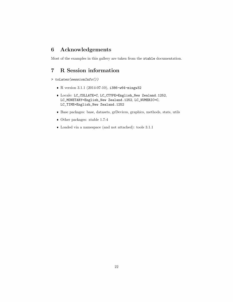
6 Acknowledgements

Most of the examples in this gallery are taken from the xtable documentation.

7 R Session information

> toLatex(sessionInfo())

� R version 3.1.1 (2014-07-10), i386-w64-mingw32

� Locale: LC_COLLATE=C, LC_CTYPE=English_New Zealand.1252,LC_MONETARY=English_New Zealand.1252, LC_NUMERIC=C,LC_TIME=English_New Zealand.1252

� Base packages: base, datasets, grDevices, graphics, methods, stats, utils

� Other packages: xtable 1.7-4

� Loaded via a namespace (and not attached): tools 3.1.1

22

Documents

xtableGallery-2