Embed Size (px)
Citation preview

Xpander: Towards Optimal-Performance Datacenters
Asaf Valadarsky∗
[email protected] Shahaf†
[email protected] Dinitz‡
Michael Schapira∗
AbstractDespite extensive efforts to meet ever-growing demands,today’s datacenters often exhibit far-from-optimal perfor-mance in terms of network utilization, resiliency to failures,cost efficiency, incremental expandability, and more. Con-sequently, many novel architectures for high performancedatacenters have been proposed. We show that the benefitsof state-of-the-art proposals are, in fact, derived from thefact that they are (implicitly) utilizing ”expander graphs”(aka expanders) as their network topologies, thus unveil-ing a unifying theme of these proposals. We observe, how-ever, that these proposals are not optimal with respect toperformance, do not scale, or suffer from seemingly insur-mountable deployment challenges. We leverage these in-sights to present Xpander, a novel datacenter architecturethat achieves near-optimal performance and provides a tan-gible alternative to existing datacenter designs. Xpander’sdesign turns ideas from the rich graph-theoretic literatureon constructing optimal expanders into an operational real-ity. We evaluate Xpander via theoretical analyses, extensivesimulations, experiments with a network emulator, and animplementation on an SDN-capable network testbed. Ourresults demonstrate that Xpander significantly outperformsboth traditional and proposed datacenter designs. We dis-cuss challenges to real-world deployment and explain howthese can be resolved.
1 IntroductionThe rapid growth of Internet services is placing tremen-dous demands on datacenters. Yet, as evidenced by the ex-tensive research on improving datacenter performance [24,25, 6, 48, 52, 23, 45], today’s datacenters often exhibit far-from-optimal performance in terms of network utilization,resiliency to failures, cost efficiency, amenability to incre-mental growth, and beyond.
1.1 The Secret to High PerformanceWe show that state-of-the-art proposals for next-gener-ation datacenters, e.g., low-diameter networks such as SlimFly [9], or random networks like Jellyfish [48], have an im-plicit unifying theme: utilizing an “expander graph” [26] as
∗School of Computer Science and Engineering, The Hebrew Universityof Jerusalem, Israel†Dept. of Mathematics, The Hebrew University, Jerusalem, Israel‡Department of Computer Science, Johns Hopkins University, USA
the network topology and exploiting the diversity of shortpaths afforded by expanders for efficient delivery of datatraffic. Thus, our first contribution is shedding light on theunderlying reason for the empirically good performance ofpreviously proposed datacenter architectures, by showingthat these proposals are specific points in a much larger de-sign space of “expander datacenters”. We observe, how-ever, that these points are either not sufficiently close to op-timal performance-wise, are inherently not scalable, or facesignificant deployment and maintenance challenges (e.g., interms of unpredictability and wiring complexity).
We argue that the quest for high-performance datacen-ter designs is inextricably intertwined with the rich bodyof research in mathematics and computer science on build-ing good expanders. We seek a point in this design spacethat offers near-optimal performance guarantees while pro-viding a practical alternative for today’s datacenters (interms of cabling, physical layout, backwards compatibilitywith today’s protocols, and more). We present Xpander, anovel expander-datacenter architecture carefully engineeredto achi-eve both these desiderata.
Importantly, utilizing expanders as network topologieshas been proposed in a large variety of contexts, rang-ing from parallel computing and high-performance comput-ing [49, 15, 14, 9] to optical networks [41] and peer-to-peernetworks [40, 39]. Our main contributions are examiningthe performance and operational implications of utilizingexpanders in the datacenter networking context, and seek-ing optimal design points in this specific domain (namely,Xpander). Indeed, despite the large body of research on ex-panders, many aspects of using expanders as datacenter net-works (e.g., throughput-related performance measures, spe-cific routing and congestion control protocols, deploymentcosts, incremental growth, etc.) remain little understood.We next elaborate on expanders, expander datacenters, andXpander.
1.2 Why Expanders?
Intuitively, in an expander graph the total capacity from anyset of nodes S to the rest of the network is large with re-spect to the size of S. We present a formal definition ofexpanders in Section 2. Since this implies that in an ex-pander every cut in the network is traversed by many links,traffic between nodes is (intuitively) never bottlenecked ata small set of links, leading to good throughput guarantees.Similarly, as every cut is large, every two nodes are (intu-itively) connected by many edge-disjoint paths, leading to
1

high resiliency to failures. We validate these intuitions inthe datacenter context.
Constructing expanders is a prominent research threadin both mathematics and computer science. In particular,building well-structured, deterministic expanders has beenthe subject of extensive study (see, e.g., [34, 32, 43]).
1.3 Why Expander Datacenters?We refer to datacenter architectures that employ an ex-pander network topology as “expander datacenters”. Weevaluate the performance of various expander datacentersthrough a combination of formal analyses, extensive flow-level and packet-level simulations, experiments with themininet network emulator, and implementation on an SDN-capable network testbed (OCEAN [3]).
Our results reveal that expander datacenters achieve near-optimal network throughput, significantly outperformingtraditional datacenters (fat trees [6]). We show, in fact, thatexpander datacenters can match the performance of today’sdatacenters with roughly 80−85% of the switches. Beyondthe above improvements in performance, our results estab-lish that expander datacenters are significantly more robustto network changes than today’s datacenters.
Studies of datacenter traffic patterns reveal tremendousvariation in traffic over time [7]. Unfortunately, a networktopology that fares well in one traffic scenario might failmiserably in other scenarios. We show that expander dat-acenters are robust to variations in traffic. Specifically, anexpander datacenter provides close-to-optimal performanceguarantees with respect to any (even adversarially chosen!)traffic pattern. We show, moreover, that no other networktopology can do better. The performance of expander dat-acenters also degrades much more gracefully than fat treesin the presence of network failures.
Alongside the above merits, expander datacenters, unliketoday’s rigid datacenter networks, can be incrementally ex-panded to any size while preserving high performance, thusmeeting the need to constantly grow existing datacenters.
1.4 Why Xpander?While our results indicate that expander datacenters univer-sally achieve high performance, different expander datacen-ters can differ greatly both in terms of the exact level ofperformance attained, and in terms of their deployability.We thus seek a point in the space of expander datacentersthat achieves near-optimal performance while presenting apractical alternative for today’s datacenters. We presentXpander, which we regard as a good candidate for sucha point. We evaluate Xpander’s performance guarantees,showing that it achieves the same level of performance asrandom networks, the current state-of-the-art with respectto performance [48, 47, 27] (but which suffer from severeimpediments to deployment, as discussed later), and thatit outperforms low-diameter datacenter designs (namely,Slim-Fly [9]).
We analyze the challenges facing the deployment of Xpa-nder in practice through detailed investigations of variousscenarios, from “container datacenters” to large-scale dat-acenters. Our analyses provide evidence that Xpander is
realizable with monetary and power consumption costs thatare comparable or lower than those of today’s prevalent dat-acenter architectures and, moreover, that its inherent well-structuredness and order make wiring Xpanders manage-able (avoiding, e.g., the inherent unstructuredness and com-plexity of random network designs a la Jellyfish [48]).
1.5 OrganizationWe provide a formal exposition of expanders and expanderdatacenters in Section 2, and of Xpander in Section 3. Weshow that expander datacenters such as Xpander indeed at-tain near-optimal performance in Section 4, matching theperformance of randomly networked datacenters. We com-pare Xpander to fat trees [6] and Slim Fly [9] in Sections 5and 6, respectively. We discuss deployment challenges andsolutions in Section 7, and related work in Section 8. Weconclude in Section 9.
See more details on Xpander in the Xpander project web-page [5].
2 Expander DatacentersWe provide below a formal exposition of expanders. Wediscuss past proposals for high-performance datacentersand explain why these are, in fact, “expander datacenters”.
Consider an (undirected) graph G = (V,E), where Vand E are the vertex set and edge set, respectively. For anysubset of vertices S, let |S| denote the size of S, let ∂(S)denote the set of edges leaving S, and let |∂(S)| denote thesize of ∂(S). Let n denote the number of vertices in V (thatis, |V |). The edge expansion EE(G) of a graph G on nvertices is EE(G) = min|S|≤n
2
|∂(S)||S| . We say that a graph
G is d-regular if the degree of each vertex is exactly d. Wecall a d-regular graph G an expander if EE(G) = c · dfor some constant c > 0. We note that the edge expansionof a d-regular graph cannot exceed d
2 .1 Constructions ofexpanders whose edge expansion (asymptotically) matchesthis upper bound exist (see more below).
We refer to datacenters that rely on an expander graph astheir network topology as “expander datacenters”. We con-sider two recent approaches to datacenter design that havebeen shown to yield significantly better performance thanboth today’s datacenters and many other proposals: low-diameter networks, e.g., Slim Fly [9], and randomly net-worked datacenters, e.g., Jellyfish [48]. We observe thatthese two designs are, in fact, expander datacenters. Weshow in the subsequent sections that this is indeed what ac-counts for their good performance.
Randomly networked datacenters. Recent studies [48,47] show that randomly networked datacenters achieveclose-to-optimal performance guarantees. Indeed, to date,randomly networked datacenters remain the state-of-the-art (performance-wise) in terms of network throughput,resilien-cy to failures, incremental expandability, and more.Our results for expander datacenters suggest that these mer-its of randomly-wired, d-regular, datacenters are derived
1This is what is achieved by a random bisection and thus the worstbisection is no better.
2

from the fact that they achieve near-optimal edge expansion(close to d
2 ), as established by classical results in randomgraph theory [11, 20].
Unfortunately, the inherent unstructuredness of randomgraphs makes them hard to reason about (diagnose and trou-bleshoot problems, etc.) and build (e.g., cable), and thusposes serious, arguably insurmountable, obstacles to theiradoption. Worse yet, as with any probabilistic construct,the good traits of random graphs are guaranteed only withsome probability. Hence, while utilizing random networktopologies in datacenters is an important thought experi-ment, the question arises: Can a well-structured and deter-ministic construction achieve the same benefits always (andnot probabilistically)? We show later that Xpander indeedaccomplishes this.
Low-diameter datacenters. Slim Fly [9] (SF) leveragesa graph-theoretic construction of low-diameter graphs [35](of diameter 2 or 3). Intuitively, by decreasing the diame-ter, less capacity is wasted when sending data, and henceoverall performance is higher. As shown in [9], SF outper-forms both existing and proposed datacenter architectures,but performs worse than random network topologies. Thefollowing result (proven in [18]) shows that SF is, in fact, agood expander.
Theorem 2.1. [18] A Slim-Fly network of degree d anddiameter 2 has edge expansion at least d3 − 1.
This result suggests that SF’s good edge expansion may,in fact, be the explanation for its good performance, andnot its low diameter. Indeed, our findings (see Section 6)suggest that by optimizing the diameter-size tradeoff, SlimFly sacrifices a small amount of expansion, which leads toworse performance than random networks (and Xpander)as the network gets larger. Worse yet, the low diameter ofSF imposes an extremely strict condition on its size (as afunction of port count of each switch), imposing, in turn,a strict limit on the scalability of Slim Fly. Xpander, incontrast, can be constructed for virtually any given switchport-count and network size, as discussed in Section 6.
Other expander datacenters. A rich body of literaturein mathematics and computer science deals with construc-tions of expanders, e.g., Margulis’s construction [34], alge-braic constructions [32], and constructions that utilize theso-called “zig-zag product” [43]. Such constructions canbe leveraged as network topologies in the design of ex-pander datacenters. For example, our construction of theXpander datacenter topology utilizes the notion of 2-liftinga graph, introduced by Bilu and Linial [10, 33] (see Sec-tion 3). However, as evidenced by the above discussion, dif-ferent choices of expanders can yield different performancebenefits and greatly differ in terms of deployability. We nextdiscuss the Xpander architecture, designed to achieve near-optimal performance and deployability.
3 Xpander: Overview and DesignIn light of the limitations of past proposals, our goal is toidentify a datacenter architecture that achieves near-optimalperformance yet overcomes deployment challenges. We
(a) (b) (c)
Figure 1: Illustration of 2-Lift
Figure 2: An Xpander topology sketch
next present the Xpander datacenter design, and show thatit indeed accomplishes these desiderata.
3.1 Network TopologyLifting a graph. Consider the graph G depicted in Fig-ure 1(a). Our construction of Xpander leverages the ideaof “lifting” a graph [10, 15]. We start by explaining 2-lifts.A 2-lift of G is a graph obtained from G by (1) creatingtwo vertices v1 and v2 for every vertex v in G; and (2) forevery edge e = u, v in G, inserting two edges (a match-ing) between the two copies of u (namely, u1 and u2) andthe two copies of v (namely, v1 and v2). Figure 1(b) is anexample of a 2-lift of G. Observe that the pair of verticesv1 and v2 can be connected to the pair u1 and u2 in twopossible ways, described by the solid and dashed lines inFigure 1(c). When the original graph G is an expander, the2-lift of G obtained by choosing between every two suchoptions at random is also an expander with high probabil-ity [10]. Also, these simple random choices can be deran-domized, i.e., the same guarantee can be derived in a deter-ministic manner [10].
2-lifting can be generalized to k-lifting for arbitrary val-ues of k in a straightforward manner: create, for every ver-tex v in G, k vertices, and for every edge e = u, v inG, insert a matching between the k copies of u and the kcopies of v. As with 2-lifting, k-lifting an expander graphvia random matchings results in a good expander [15, 19].We are unaware of schemes for de-randomizing k-lifts fork > 2. However, we show empirically that k-lifts for k > 2can also be derandomized.
Xpander’s network topology. To construct a d-regularXpan-der network, where each node (vertex) represents atop-of-rack (ToR) switch, and d represents the number ofports per switch used to connect to other switches (all otherports are connected to servers within the rack), we do the
3

Figure 3: Division of an Xpander into Xpander-pods.
following: start with the complete d-regular graph on d+ 1vertices and repeatedly lift this graph in a manner that pre-serves expansion.
Although lifting a graph (at least) doubles the numberof nodes, we show in Section 4.3 how Xpander topologiescan be incrementally grown (a single node at a time) to anydesired number of nodes while retaining good expansion.
Selecting the “right” Xpander. Today’s rigid datacen-ter network topologies (e.g., fat trees) are only defined forvery specific combinations of number of nodes (switches)n and per-node degree (port count) d. An Xpander, in con-trast, can be generated for virtually any combination of nand d by varying the number of ports used for inter-switchconnections (and, consequently, for switch-to-server con-nections), or through the execution of different sequencesof k-lifts. The choice of specific Xpander depends on theobjectives of the datacenter designer, e.g., minimizing net-work equipment (switches/links) while maintaining a cer-tain level of performance. See Section 5 for a few more de-tails. To select the “right” Xpander, the datacenter architectcan play with Xpander’s construction parameters to gener-ate several Xpander networks of the desired size, numberof servers supported, etc., and then measure their perfor-mance, in terms of expansion2 and throughput, to identifythe best candidate.
3.2 Xpander’s Logical Organization
Observe that, as described in Figure 2, an Xpander net-work can be regarded as composed of multiple “meta-nodes” such that (1) each meta-node consists of the samenumber of ToRs, (2) every two meta-nodes are connectedvia the same number of links, and (3) no two ToRs withinthe same meta-node are directly connected. Each meta-node is, essentially, the group of nodes which correspond toone of the original d + 1 nodes. Also, an Xpander can nat-urally be divided into smaller Xpanders (“Xpander-pods”),each of the form depicted in Figure 2, such that each podis simply a collection of meta-nodes. See Figure 3 for anillustration of an Xpander with 9 meta-nodes (i.e., d = 8),divided into 3 equal-sized pods. Observe that division of
2Importantly, computing edge expansion is, in general, computation-ally hard [30], yet edge expansion can be approximated via the tractablenotion of spectral gap [26].
an Xpander into Xpander-pods need not be into pods of thesame size.
We show in Section 7 how this “clean” structure can beleveraged to tame cabling complexity.
3.3 Routing and Congestion Control
We show that traditional routing with ECMP and TCP con-gestion control are insufficient to exploit Xpander’s richpath diversity. Xpander thus, similarly to [48], employsmultipath routing via K-shortest paths [53, 17] and MPTCPcongestion control [51]. K-shortest paths can be imple-mented in several ways, including OpenFlow rule match-ing [36], SPAIN [37], and MPLS tunneling [44].
4 Near-Optimal PerformanceWe show that Xpander achieves near-optimal performancein terms of throughput and bisection bandwidth guarantees,robustness to traffic variations, resiliency to failures, incre-mental expandability, and path lengths. Both our simu-lations and theoretical results benchmark Xpander againsta (possibly unattainable) theoretical upper bound on per-formance for any datacenter network. To benchmark alsoagainst the state-of-the-art, we show that Xpander matchesthe near-optimal performance of random datacenter archi-tectures, demonstrated in [48, 47]. We will later explainhow Xpander’s design mitigates the deployment challengesfacing randomly networked datacenters (Section 7).
We note that Xpander’s near-optimal performance ben-efits are derived from utilizing a nearly optimal expandernetwork topology [10]. Indeed, our results for Xpander’sperformance extend to all expander datacenters whose d-regular network topology exhibits near-optimal edge ex-pansion (i.e., edge expansion close to d
2 ), such as randomnetworks and algebraic constructions of expanders [32].To simplify exposition, our discussion below focuses onXpander and Jellyfish [48].
4.1 Near-Optimal Throughput
4.1.1 Simulation Results
Simulation framework. We ran simulations on Xpandernetworks for many choices of number of nodes n and node-degree d. The node degree d in our simulations refers onlyto the number of ports of a switch used to connect to otherswitches and not to switch-to-server ports. We henceforthuse k to refer to the total number of ports at each switch(used to connect to either other switches or servers). Wetested every even degree in the range 6-30 and up to 600switches (and so thousands of servers) using a flow-levelsimulator described below. As our simulations show theexact same trends for all choices of parameters, we dis-play figures for selected choices of n and d. To validatethat Xpanders indeed achieve near-optimal performance,we benchmarked Xpanders also against Jellyfish’s perfor-mance (averaged over 10 runs). We also simulate largeXpander networks, the largest supporting 27K servers, us-ing the MPTCP packet simulator [2].
4

(a) k = 14. There are 4 servers placed under each switch (b) k = 18. There are 4 servers placed under each switch.
Figure 4: Results for all-to-all throughput
(a) k = 8. There are two servers places under each switch. (b) k = 14. There are 4 servers placed under each switch.
Figure 5: Results for all-to-all throughput under ECMP
We compute the following values for every networktopology considered: (1) the maximum all-to-all through-put, that is, the maximum amount of flow-level traffic αthat can be concurrently routed between every two switchesin the network without exceeding link capacities (see for-mal definition in Section 4.1.2); (2) the throughput underskewed traffic matrices (elephants and mice); (3) the all-to-all throughput under ECMP routing coupled with TCPcongestion control; and (4) the all-to-all throughput un-der K-shortest-paths routing coupled with MultiPath TCP(MPTCP) congestion control.
Intuitively, (1)+(2) capture the maximum flow achievablewhen the full path diversity of Xpander, Jellyfish and addi-tional expander based constructions can be exploited, (3)captures the extent to which Xpander’s path diversity canbe utilized via today’s standard routing and congestion con-trol protocols and (4) captures the packet-level performanceunder Xpander’s routing and congestion control. Thus, oursimulations quantify both the best (flow-level) throughputachievable and how closely Xpander’s routing and conges-tion control protocols approach this optimum.
To compute (1)+(2)+(3), our simulations ran the CPLEXoptimizer [1] on a 64GB, 16-core server. Our simulationframework is highly-optimized, allowing us to investigatedatacenter topologies with significantly higher parametervalues (numbers of switches n, servers, and per switch portcounts d) than past studies. To compute the throughput un-der K-shortest paths and MPTCP (4) we use the MPTCPpacket-level simulator [2]. We later validate these resultsusing the mininet network emulator [29] (Section 5.3) andsmall-scale deployment (Section 5.4).
Expanders provide near-optimal network throughput.Figure 4 describes our representative results for all-to-allthroughput (the y-axis) as a function of the number ofservers in the network (the x-axis) when the switch’s inter-switch degree (ports used to connect to other switches) isd = 10 (left) and d = 14 (right). The results are normal-ized by the theoretical upper bound on the throughput ofany network [47]. To show that our results are not specificto Xpander of Jellyfish, but extend to all network topolo-gies with comparable edge expansion, Figure 4 also plotsthe performance of 2-lifts of the algebraic construction ofexpanders due to Lubotzky et al. [32], called “LPS”. Toevaluate LPS-based expanders of varying sizes, we gener-ated an LPS expander and then repeatedly 2-lifted it to gen-erate larger expanders (the subscript in the figure specifiesthe number of nodes in the initial LPS expander, before 2-lifting).
Clearly, the achieved performance for all evaluated ex-panders is essentially identical and is close to the (possi-bly unattainable) theoretical optimum. Note that there is adip in the performance, but as explained in [47], this is afunction of how the upper bound, which at this point be-comes unattainable, is calculated. Even here, however, bothXpander and Jellyfish remain fairly close to the (unattain-able) upper bound. We show in the subsequent sections thatthis level of performance is above that of both today’s data-centers and Slim Fly [9].
While the network throughput of expanders is near-optimal, how can this be achieved in practice?
5

(a) Xpander (b) Jellyfish
Figure 6: Results for K-Shortest & MPTCP with K = #Subflows. 6 servers placed under each 36-port switch.
ECMP and TCP are not enough. We evaluate all-to-all throughput under ECMP (and TCP) for many choicesof n and d. Figure 5 shows that while deterministic con-structions consistently outperform random graphs (JF) by∼10%, ECMP utilizes ∼80% of the network capacity atbest, and only 60-70% most of the time. So, as with ran-dom datacenter topologies [48], ECMP’s throughput guar-antees for expanders are disappointing. We point out thatthis is not at all surprising as while fat-trees provide richdiversity of shortest-paths between any two ToR switches,in an expander two neighbouring switches, for instance, areconnected via but a single shortest-path (the edge betweenthem). As before, the sudden dip in performance in the fig-ure is due to how the upper bound from [47] is calculated.
Solution: K-shortest-paths and MPTCP. One approachto overcoming ECMP’s low throughput guarantees is usingthe K-shortest paths algorithm [53, 17] and MPTCP [51].
The results for other choices of d and n exhibit the sametrends. Our results show that when K ≥ 6 and the numberof MPTCP subflows equals K, the server average through-put is very close to its maximum outgoing capacity.
We measured, using the MPTCP packet-level simula-tor [2], the average per-server throughput (as a percentageof the servers’ NIC rate) for different choices of parame-ter K in K-shortest paths. Specifically, we measured: (1)the all-to-all throughput when the number of MPTCP sub-flows is 8 (the recommended value [48, 51]), and (2) whenthe number of subflows is K, we use d = 30 and up to496 switches (or nearly 3K servers). Our results show thatwhen K ≥ 6 the all-to-all throughput is very close to the(possibly unattainable) theoretical upper bound on all-to-allthroughput in [47]. We present our results for d = 10, av-eraged over 10 runs for Jellyfish, in Figures 6 and 7. Theresults for other values of d exhibit the same trends. Ourresults show that when K ≥ 6 and the number of MPTCPsubflows equals K, the server average throughput is veryclose to its maximum outgoing capacity.
We show below, through additional simulations, exper-iments with Mininet and a tesbed deployment (see Sec-tions 5.3 and 5.4), that this indeed provides the desired per-formance. As discussed in [48], K-shortest path can be im-plemented in several ways, including OpenFlow rule match-ing [36], SPAIN [37], and MPLS tunneling [44].
(a) k = 14. There are 4 servers placed under each switch.
Figure 7: Results for K-Shortest & MPTCP with#Subflows = K
Throughout the rest of the paper, unless stated otherwise,we will use K-shortest paths with a value of K = 8.
Results for skewed traffic matrices. We also evaluated thethroughput of Xpander for skewed traffic matrices, whereeach of T randomly-chosen pairs of nodes wishes to trans-mit a large amount of traffic, namely β units of flow, andall other pairs only wish to exchange a single unit of flow(as in the all-to-all scenario). We simulated this scenariofor network size n = 250, every even d = 2, 4, . . . , 24,and all combinations of T ∈ 1, 6, 11, . . . , 46 and β ∈4, 40, 400.
For each choice of parameters, we computed the net-work throughput α, that is, the maximum fraction of eachtraffic demand that can be sent through the network con-currently without exceeding link capacities. The resultsare again normalized by a simple theoretical (and unattain-able) upper bound on any network’s throughput for thesetraffic demands (calculation omitted). Our simulation re-sults for skewed traffic matrices show that the throughputachieved by Xpander is almost always (over 96% of re-sults) within 15% of the optimum throughput, and typicallywithin 5− 10% from the theoretical optimum. See Table 1for a breakdown of the results. We use the MPTCP simu-lator to compare Xpander to fat trees in Section 5, showingthat Xpander provides the same level of performance withmuch fewer switches.
6

Distance from Optimum Xpander JellyFishthroughput<80% <1% <1%80% ≤ throughput <85% 2.3% 2.3%85% ≤ throughput <90% 16.14% 16.14%90% ≤ throughput <95% 44.48% 48.03%95% ≤ throughput 36.61% 32.67%
Table 1: Distance of throughput from the (unattainable)optimum for various combinations of β, T, d.
Figure 8: Throughput under link failures.
4.1.2 Theoretical Results
Near-optimal bisection bandwidth. Recall that bisectionbandwidth is the minimum number of edges (total capac-ity) traversing a cut whose sides are of equal size [54], orformally minS:|S|=n
2|∂(S)| using the notation from Sec-
tion 2. Since in an expander intuitively all cuts are large,not surprisingly Xpander indeed achieves near-optimal bi-section bandwidth. Note that the bisection bandwidth ofany d-regular graph is at most n2 ·
d2 = nd
4 .3
Theorem 4.1. An Xpander graph on n vertices has bisec-tion bandwidth at least n2
(d2 −O(d3/4)
).
Proof. We know from [19] that any Xpander graph has edgeexpansion at least d
2 − O(d3/4). Thus, as bisection band-width measures the number of edges across cuts that di-vide the set of n nodes into two sets of size n
2 , it is at leastn2
(d2 −O(d3/4)
).
Moreover, the definition of edge expansion of a graph G,EE(G), immediately implies the bisection bandwidth of anarbitrary d-regular graph is at least n2 ·EE(G), and so evenin an arbitrary d-regular expander the bisection bandwidthmust be quite high.
Near-optimal throughput. We consider the following sim-ple fluid-flow model of network throughput [27]: A networkis represented as a capacitated graph G = (V,E), wherevertex set V represents (top-of-rack) switches and edge setE represents switch-to-switch links. All edges have a ca-pacity of 1. A traffic matrix T specifies, for every two ver-tices (switches) u, v ∈ V , the total amount of requestedflow Tu,v from servers connected to u to servers connectedto v. The network throughput under traffic matrix T is de-fined as the maximum value α such that α · Tu,v flow can
3This is what is achieved by a random bisection and thus the worstbisection is no better.
be routed concurrently from each vertex u to each vertexv without exceeding the link capacities. For a graph G andtraffic matrix T , let α(G,T ) denote the throughput ofG un-der T . We refer to the scenario in which Tu,v = 1 for everyu, v ∈ V (i.e. every node aims to send 1 unit of flow to ev-ery other node) as the “all-to-all setting”. We will slightlyabuse notation and let α(G) denote the throughput of G inthe all-to-all setting.
We present several simple-to-prove results on thethroughput guarantees of expander datacenters. Beyondaccounting for Xpander’s good performance, these resultsalso account for the good performance of other expanderdatacenters, e.g., Jellyfish and Slim Fly. While possiblyfolklore, to the best of our knowledge, these results do notappear to have been stated or proven previously. We thusinclude them here for completeness.
Theorem 4.2. In the all-to-all setting, the throughput ofa d-regular expander G on n vertices is within a factor ofO(log d) of that of the throughput-optimal d-regular graphon n vertices.
Proof. Let G∗ be an arbitrary d-regular graph on n ver-tices. A simple argument (omitted) shows that in any d-regular graph, from any node u there are Ω(n) other nodesat distance at least Ω(logd n) from u. Call these nodesF (u). If we send α(G∗) flow between each pair of nodes,the total capacity used (i.e., the sum over all edges of theflow traversing the edge) is at least
∑u∈V
∑v∈F (u) α(G∗)·
Ω(logd n) = Ω(α(G∗) ·n2 logd n). Since the total capacityis at most nd
2 , this implies that α(G∗) ≤ O(
dn logd n
)=
O(d log dn logn
).
On the other hand, we can lower bound α(G) usingthe flow-cut gap from [30, 8]. This theorem says that thethroughput is at least 1
O(logn) times the minimum (over allcuts) of the capacity across the cut divided by the demandacross the cut. When applied to the all-to-all setting, thisimplies that
α(G) ≥ 1
O(log n)min
S⊆V :|S|≤n/2
|∂(S)||S|(n− |S|)
By the definition of edge expansion, we know that |∂(S)| ≥EE(G)|S|, and since G is an expander we know thatEE(G) ≥ Ω(d). Combining these, we get that α(G) ≥
1O(logn)
dn , and thus α(G∗) ≤ O(log d)α(G).
The next two results, when put together, show that ex-panders (and so also Xpander) are, in a sense, the networktopology most resilient to adversarial traffic scenarios.
Theorem 4.3. For any traffic matrix T and d-regular ex-pander G on n vertices, α(G,T ) is within a factor ofO(log n) of that of the throughput optimal d-regular graphon n vertices with respect to T .
Proof. We can again use the flow-cut gap of [30, 8].For a subset S ⊆ V with |S| ≤ n/2, let T (S) =∑u∈S
∑v 6∈S Tu,v be the total demand across S. Let G∗ be
7

(a) k = 32. There are 8 servers placed under each switch. (b) k = 48. There are 12 servers placed under each switch.
Figure 9: Results for avg. path length
an arbitrary d-regular graph on n vertices. Then the flow-cut gap guarantees that for any graph G′,
1
O(log n)min|S|≤n/2
|∂(S)|T (S)
≤ α(G′, T ) ≤ min|S|≤n/2
|∂(S)|T (S)
Now we can upper bound the throughput ofG∗ by notingthat |∂(S)| ≤ d|S|, so α(G∗, T ) ≤ min|S|≤n/2
d|S|T (S) . On
the other hand, we can lower bound the throughput of G bynoting that |∂(S)| ≥ |S| × EE(G) ≥ Ω(d|S|) (since G isan expander), and thus
α(G,T ) ≥ 1
O(log n)min|S|≤n/2
Ω(d|S|)T (S)
Thus α(G∗, T ) ≤ O(log n)α(G,T ), as claimed.
Theorem 4.4. For any d-regular graph G on n vertices,there exists a traffic matrix T and a d-regular graph G∗ onn vertices such that α(G∗, T ) ≥ Ω(logd n) · α(G,T ).
Proof. Let π : V → V be a random permutation. Let G∗
be the graph obtained by including an edge u, v if andonly if π−1(u), π−1(v) is an edge in G (i.e. G∗ is just arandom isomorphism ofG). Let T be the traffic matrix suchthat Tu,v = 1 if u, v ∈ E(G∗) and Tu,v = 0 otherwise.Then clearly α(G∗, T ) = 1, since the traffic demands areexactly the edges of G∗.
To analyze what happens inG, note that sinceG has max-imum degree d, the average distance between two nodesis Ω(logd n). So since π is a random permutation, theexpected distance in G between two nodes that are adja-cent in G∗ is also Ω(logd n). So by linearity of expec-tations, E
[∑u,v:Tu,v=1 distG(u, v)
]≥ Ω(dn logd n).
Thus we can fix some π where this is true, i.e. where -∑u,v:Tu,v=1 distG(u, v) ≥ Ω(dn logd n). Then if we
send α(G,T ) units of flow for every traffic demand, thetotal capacity used up is at least Ω(α(G,T ) ·dn logd n). Onthe other hand, the total capacity in G is only |E| = dn/2.Thus α(G,T ) ≤ O(1/ logd n). Putting this together, weget that α(G,T ) ≤ O
(1
logd n
)· α(G∗, T ).
4.2 Near-Optimal Resiliency to FailuresWe begin with a straightforward observation (proven belowfor completeness): in any d-regular expander datacenter, thenumber of edge-disjoint paths between any two vertices isexactly d.
Theorem 4.5. In any d-regular expander with edge expan-sion at least 1, any two vertices are connected by exactly dedge-disjoint paths.
Proof. Let u, v ∈ V . By Menger’s Theorem, the number ofedge-disjoint paths from u to v is equal to the minimum cutseparating u and v. Consider any cut (S, S) with u ∈ S andv ∈ S. Without loss of generality, suppose |S| ≤ n
2 . Then,if |S| ≥ d, since the edge expansion is at least 1 the numberof edges across the cut is at least EE(G) · |S| ≥ d. If|S| < d, then since each node in S has degree d the numberof edges crossing the cut must be at least d|S|−|S|(|S|−1),which for |S| between 1 and d− 1 is at least d. Thus, everycut separating u and v has at least d edges, and so there ared edge-disjoint paths between u and v.
Since this is the maximum possible number of such pathsin a d-regular graph, Xpander’s network topology (or anyother “sufficiently good” expander) provides optimal con-nectivity between any two communicating end-points andcan thus withstand the maximum number of link-failures(specifically, d− 1) without disconnecting two switches.
We next turn to experimental evaluation. We compute theall-to-all server-to-server throughput in Xpander and Jelly-fish after failing X links uniformly at random, where Xranges from 0% to 30% in increments of 3%. We repeatedthis for Xpander networks of many sizes and node-degrees.Figure 8 shows our (representative) results for Xpander andJellyfish of 708 servers and 236 14-ports switches (withone switch port left unused). As shown in the figure, thethroughput of Xpander degrades linearly with the failurerate. We show in Section 5 through both flow-level andpacket-level simulations that the throughput of Xpandersindeed dominates that of fat trees (both with and withoutfailures).
Intuitively, this linear dependence on the failure rate isnatural. If the probability of link failure is p, then after fail-ures the graph is similar to a ((1 − p)d)-regular Xpander.This is because for each cut S the number of edges across it(|∂(S)|) before failure was large, owing to G being an ex-pander, and so after failure the number of edges across the
8

Figure 10: Throughput under incremental expansion fork = 32, incrementally adding 1 switch and 8 servers ateach step.
cut is tightly concentrated around its expectation, which is(1− p)|∂(S)|.
4.3 Incremental Expandability
Companies such as Google, Facebook and Amazon con-stantly expand existing datacenters to meet ever-growingdemands. A significant advantage of random graphs (i.e.,Jellyfish [48]) over traditional datacenter topologies (e.g.,fat trees) is the ability to incrementally expand the networkwithout having to leave many ports unused etc.
We present a deterministic heuristic for incrementally ex-panding a d-regular expander datacenter with few wiringchanges when adding a new node (ToR): To add a newnode to the datacenter, disconnect d2 existing links and con-nect the d incident nodes (ToRs) to the newly added node(recall that d is the number of ports used to connect toother switches). Observe that this is indeed the minimalrewiring needed as at least d
2 links must be removed to“make room” for the new switch. The key challenge is se-lecting the links to remove. Intuitively, our heuristic goesover all links and quantifies the loss in edge expansion fromremoving each link, and then removes the d
2 links whose re-moval is the least harmful in this regard. Importantly, sincecomputing edge expansion is, in general, computationallyhard [30], our heuristic relies on the tractable notion ofspectral gap [26], which approximates the edge expansion.Appendix B for a technical exposition of this heuristic.
We compute the all-to-all throughput of topologies thatare gradually expanded from the complete d-regular graphusing our deterministic incremental growth algorithm, andcompare them to the theoretical upper bound on thethroughput of any d-regular datacenter network.
Figure 10 shows the all-to-all throughput results for anXpander with 32-port switches. At each size-increment-step, one switch (and 8 servers) is added, thus graduallygrowing the datacenter network from 200 servers to 900servers. As shown in Figure 10, all Xpander datacen-ter networks obtained in this manner achieve near-optimalthroughput. We compare Xpander against the incrementalgrowth of Jellyfish, as presented in [48].
Figure 11: Results for diameter. We use k = 48 switcheswith 12 servers placed under each switch.
fat treeDegree #Switches #Servers Throughput
8 80% 100% 121%10 100% 100% 157%12 80.5% 100% 103%14 96% 103% 122%16 80% 100% 120%18 90% 100% 137%20 80% 100% 118%22 89% 102% 121%24 80% 100% 111%
Table 2: Xpanders vs. fat trees (FT), flow-level simula-tions. Percentages are Xpander/FT.
4.4 Short Path-Lengths and Diameter
As shown in Figure 9, all evaluated Xpander (and Jellyfish)networks exhibit the same average shortest path lengths andare, in fact, usually within 5% of the lower bound on aver-age path length in [13]. (Results for many other choices ofn and d lead to the same conclusion.) Thus, Xpander effec-tively minimizes the average path length between switches.
A straightforward argument (omitted) shows thatdlogd ne is a lower bound on the diameter of a d-regulargraph. All Xpanders evaluated are within just 1 hop fromthis theoretical lower bound ( Figure 11).
5 Xpander vs. Fat Tree
We next detail the significant performance benefits of Xpan-der datacenters over fat trees. We show that Xpander cansupport the same number of servers as a fat tree at the same(or better) level of performance with only about 80−85% ofthe switches. We also show that Xpander is more resilientto failures.
5.1 Better Performance, Less Equipment
We examine uniform fat tree topologies for every even de-gree (number of ports per switch) between 8 and 24. Unlikea fat tree, which is uniquely defined for a given switch port-count, Xpander gives the datacenter designer much greaterflexibility (see discussion in Section 3.1). We identify, foreach fat tree in the above range, an Xpander with muchfewer (roughly 80-85%) switches that supports the same
9

(a) d=14 (b) d=32
Figure 12: Server-to-server throughput degradation with failures. All-to-All flow level (on the left) and Random-Shufflepacket level (on the right
Fat TreeDegree #Switches #Servers Packet Simulation
Throughput32 90% 98.5% 110%48 88% 100% 102%
Table 3: Xpanders vs. fat trees, packet-level simulationresults. Percentages are Xpander/FT.
number of servers with at least the same level of server-to-server throughput.4 See details in Table 2.
5.2 Simulation Results
Throughput. We evaluate the all-to-all throughput ofXpander and fat trees. We show in Table 2 the all-to-allserver-to-server throughput in fat trees and Xpanders with-out any link failures. As can be seen in Table 2, Xpanderis able to achieve comparable, if not better, server-to-serverthroughput than fat trees even with as few as 80% of theswitches. Table 3 shows the results of extensive packetbased-simulations using the MPTCP network simulator forXpander and fat trees with k = 32 and k = 48, contain-ing 8K and 27K servers, respectively. Again, Xpandernetworks achieve similar or better performance to that offat trees, with significantly fewer switches.
To explore how Xpander and fat trees compare for othertraffic patterns, we also simulate a fat tree of 8K servers(i.e., k = 32) and its matching Xpander under the fol-lowing “Many-to-One” scenario using the MPTCP packetlevel simulator. We randomly select 10% of the serversas our destinations and for each such server we select atrandom x% of the servers to generate traffic destined forthat server, where x=1%, 1.5%, 2%, 2.5% and 3% (1% isroughly 80 servers). Table 5 presents the averaged results of4 such simulations. We conclude that, once again, Xpanderprovides the same level of performance with less networkequipment.
Robustness to failures. We compute the all-to-all server-to-server throughput in fat trees and Xpanders after fail-
4We now consider server-to-server all-to-all throughput and not switch-to-switch all-to-all throughput, since in a fat tree not all switches originatetraffic.
Percentage Of ServersRouting To Each Destination
Packet SimulationThroughput
1% 99.6%1.5% 99.3%2% 101%
2.5% 103%3% 103%
Table 5: Xpanders vs. fat trees, 10% of the servers areselected as destinations. Percentages for throughput areXpander/FT.
ing X links uniformly at random, where X ranges 0% to30% in increments of 3%. We repeated this for fat treesof all even degrees in the range 8-24 and the correspondingXpander networks from Table 2. Figure 12(a) describes our(representative) results for fat trees of degree k = 14 (vs.Xpander). We further simulate a fat tree with k = 32, con-taining 1280 switches and 8192 servers, against an Xpandercontaining 90% of the switches and 98.5% of the servers,under a random-shuffle permutation matrix after failing Slinks uniformally at random, where S ranges from 0% to30% in increments of 5%. The results of this simulationare described in Figure 12(b). Both results (flow-level andpacket-level alike) show that Xpander indeed exhibits betterresiliency to failures than fat tree. We note that the smallergap between Xpander and fat tree in the MPTCP simula-tions can be explained by the fact that the per switch degreeis higher and so naturally routing is less affected by failures.
5.3 Xpander EmulationTo show that an Xpander with significantly less switchescan achieve comparable performance to fat trees, we usedmininet [29] and the RipL-POX [4] controller to simulatefat tree [6] networks under various workloads, and for tworouting & congestion control schemes: (1) ECMP with TCPand (2) K-shortest-paths with K = 8 and MPTCP with 8subflows. We also simulated Xpanders for the same work-loads under K-shortest-paths with K = 8 and MPTCP with8 subflows. These simulations were performed on a VMrunning Ubuntu 14.04 with MPTCP kernel version 3.5.0-89 [12]. We chose, for compute and scalability constraints,
10

Tested Topology Random Shuffle One-to-Many Many-to-One Big-and-SmallAvg Max Avg Max Avg Max Avg Max
Xpander 19.66 58.86 79.52 104.03 70.09 90.88 28.66 120.21FatTree (TCP+ECMP) 26.7 102.86 80.72 89.94 80.79 91.51 42.72 220.1FatTree (MPTCP+ECMP) 17.94 105.71 78.18 138.5 69.56 91.31 31.75 180.64
Table 4: Xpander and fat trees under various traffic matrices. Values are given in seconds and indicate the averagefinishing time for transmission.
#Ports perSwitch
(Sw2Sw / Total)
#Switches(XPNDR / SF)
#Servers(XPNDR / SF)
BisectionBandwidth
Costper node
Powerper node Expansion
5 / 8 18 / 18 (100%) 54 / 54 (100%) 86% 123% 114% 77%7 / 11 48 / 50 (96%) 192 / 200 (96%) 67% 79% 81% 72%
11 / 17 96 / 98 (98%) 576 / 588 (98%) 98% 106% 104% 84%17 / 26 234 / 242 (96%) 2,106 / 2,178 (96%) 102% 102% 100% 92%19 / 29 340 / 338 (104%) 3,400 / 3,380 (104%) 103% 95% 94% 96%25 / 38 572 / 578 (99%) 7,436 / 7,541 (98%) 109% 95% 94% 102%29 / 44 720 / 722 (99%) 10,800 / 10,830 (99%) 118% 104% 102% 103%35 / 51 1080 / 1058 (102%) 17,280 / 16,928 (102%) 119% 102% 100% 101%43 / 65 1672 / 1682 (99%) 36,784 / 37,004 (99%) 117% 99% 96% 107%47 / 71 1920 / 1922 (99%) 46,080 / 46,128 (99%) 122% 103% 101% 108%55 / 83 2688 / 2738 (96%) 75,264 / 76,664 (98%) 119% 91% 88% 112%
Table 6: Xpander vs. Slim-Fly. The first column specifies the number of ports per switch used for switch-to-switch andthe total port count (for both Xpander and SF). Percentages are Xpander/SF.
Scenario Min Max AverageRandom Shuffle 234% 83% 135%One-to-Many 94% 138% 123%Many-to-One 115% 86% 92%
Table 7: Results for the physical simulations, all values arethe averaged value of Xpander/FatTree.
to evaluate a fat tree network of degree 8, which contains80 switches and 128 servers. We tested against this fat treetopology the corresponding Xpander datacenter from Ta-ble 2, which contains only 64 switches and the same num-ber of servers. All links between switches in both networksare of capacity 1Mbps.
The workloads considered are: (1) Random Shuffle,where the 128 servers are divided into two halves, and eachmember of the first half sends a 1Mb file to a (unique) ran-domly chosen member of the other half; (2) One-to-Many,where 4 servers are randomly selected and these serverssend a 1Mb file to 10 other randomly chosen (unique) hosts;(3) Many-to-One, where 40 different servers send 1Mb fileeach to 4 servers (10 sending servers per each receivingserver); and (4) Big-And-Small, which is similar to Ran-dom Shuffle, only in addition each of 8 randomly chosenservers sends a 10Mb file to a unique other server. Our re-sults are summarized in Table 4. Observe that even with80% of the switches, Xpander provides comparable or bet-ter performance.
5.4 Implementation on a Network Testbed
To validate the above findings, we use OCEAN [3], anSDN-capable network testbed composed of 13 Pica8 Pronto3290 switches with 48 ports eac. We used the OCEAN plat-form to experimentally evaluate two datacenter networks:(1) a fat tree composed of 20 4-port switches, of which 8are top-of-rack switches, each connected to 2 servers (16servers overall), and (2) an Xpander consisting of 16 4-port switches, each connected to a single server (again, 16servers overall). Observe that while both networks supportthe same number of servers, the number of switches in theXpander is 80% of the number of switches in the fat tree (16vs. 20). Similarly, the number of links connecting switchesto other switches in the Xpander is 75% that of the fat tree(24 vs. 32). Note, however, that the network capacity perserver in Xpander is much higher as the number of ToRs ishigher (16 vs. 8), and each ToR is connected to less servers(1 vs. 2) and to more other switches (3 vs. 1). Thus, intu-itively, the Xpander can provide comparable or better per-formance with less network equipment. Our experimentson OCEAN confirm this intuition.
ECMP routing and TCP are used to flow traffic in thefat tree, whereas for the Xpander we use K-Shortest Paths,with k = 3, and MPTCP with 3 subflows (and so on eachof the 3 distinct paths between a source and a destinationthere is a separate MPTCP subflow). We evaluate the min,max, and average throughput under three different trafficscenarios: (1) random shuffle, in which every server routesto a single random destination, (2) many-to-one, in whicha randomly chosen server receives traffic from the other 15servers, and (3) one-to-many, in which a randomly chosenserver sends traffic to all other servers. To compute the
11

throughput for two communicating servers, an “endless”flow between these servers is generated using of an iperfclient and server and the averaged throughput is computedafter 10 minutes. Our results for each simulation setting areaveraged over 5 independent runs.
Table 7 shows our results for the above three traffic sce-narios (the rows) and for min, max, and average throughput(the columns), where % are Xpander/FT. Xpander achievescomparable or better results in each of the evaluated scenar-ios (again, using only 80% of the network equipment).
6 Xpander vs. Slim FlyWe also contrast Xpander with Slim Fly, a recent proposalfrom the world of high-performance computing (HPC). SFleverages a graph-theoretic construction of low-diametergraphs [35] (either diameter of 2, the situation most ex-plored in [9], or diameter of 3).
Intuitively, by decreasing the diameter, less capacity iswasted when sending data, and hence overall performanceis higher. Indeed, [9] shows that SF outperforms existingand proposed datacenter architectures, but performs worsethan random topologies, e.g., in terms of bisection band-width and resiliency to failures.
When comparing SF to Xpander, we first note that thelow diameter of SF imposes an extremely strict conditionon the relationship between the per node degree d and thenumber of nodes n: by requiring diameter 2, SF requiresd ≥ Ω(
√n). (Importantly, d here represents only the ports
used to connect a switch to other switches, and so, to sup-port servers, the actual port count must be even higher.)This imposes a strict limit on the scalability of Slim Fly.Xpander topologies, on the other hand, exist for essentiallyany combination of n and d and, in particular, can be usedfor arbitrarily large datacenters even with a fixed per-switchdegree d.
Not only is Xpander more flexible than SF in support-ing more nodes with smaller degrees, but it exhibits betterperformance than SF as the network grows, even in the de-gree/node regimes in which SF is well-defined. We usedthe simulation framework published in [9] to compare SFto Xpander in terms of performance and costs. The METISpartitioner [28] was used for approximating bisection band-width (as in [9]) and the code from [9] for cost and powerconsumption analysis (using the switch/cable values in [9]).We also computed the expansion for both categories ofgraphs using spectral gap computation, which approximatesedge expansion. See our results for Xpanders in Table 6 andfor Jellyfish in Table E15 in the Appendix.
Our findings suggest that, in fact, the good performanceof SF can be attributed to the fact that it is an expanderdatacenter. We back these empirical results with the newtheoretical result presented in Section 2, which shows thata Slim-Fly network of degree d and diameter 2 has edgeexpansion at least d
3 − 1, and is thus not too far from thebest achievalbe edge expansion of d2 .
We argue, however, that by optimizing the diameter-sizetradeoff, Slim Fly sacrifices a small amount of expansionleading to worse performance than random networks andXpander as the network gets larger. Our results reveal that
for networks with less than 100 switches, SF is a better ex-pander than both Xpander and Jellyfish and exhibits betterbisection bandwidth. This advantage is reversed as the net-work size increases and in turn Xpander and Jellyfish be-come better expanders. Our results thus both validate andshed light on the results in [9], showing why random graphs(and Xpander) outperform SF for large networks.
We also show (Table 6) that Xpander’s cost and powerconsumption are comparable to those of SF.
7 Deployment
We grapple with important aspects of building Xpander dat-acenters: (1) equipment and cabling costs; (2) power con-sumption; and (3) physical layout and cabling complexity.We first present a few high-level points and then the resultsof a detailed analysis of Xpander deployment in the contextof both small-scale (container-sized) datacenters and large-scale datcenters. We stress that our analyses are straight-forward and, naturally, do not capture all the intricaciesof building an actual datacenter. Our aim is to illustrateour main insights regarding the deployability of Xpanders,demonstrating, for instance, its significant deployability ad-vantages over random datacenter networks like Jellyfish.
Physical layout and cabling complexity. As illustrated inFigures 2 and 3, an Xpander consists of several meta-nodes,each containing the same number of ToRs and connected toeach other meta-node via the same number of cables. Notwo ToRs within the same meta-node are connected. This“clean” structure of Xpanders has important implications:First, placing all ToRs in a meta-node in close proximity(the same rack / row(s)) enables bundling cables betweenevery two meta-nodes. Second, a simple way to reasonabout and debug cabling is to color the rack(s) housing eachmeta-node in a unique color and color the bundle of cablesinterconnecting two meta-nodes in the respective two-colorstripes. See the illustration in Figure 2.
Thus, similarly to today’s large-scale datacenters [46],Xpander’s inherent symmetry allows for the taming ofcabling complexity via the bundling of cables. UnlikeXpander networks, whose construction naturally inducesthe above cabling scheme, other expander datacenters (e.g.,Jellyfish [48]) do not naturally lend themselves to suchhomogeneous bundling of cables. Our strong suspicion,backed by some experimental evidence, is that Jellyfishdoes not (in general) allow for a clean division of ToRs intoequal-sized meta-nodes where every two meta-nodes areconnected by the same number of cables (forming a match-ing), as Xpander does. Unfortunately, proving this seemshighly nontrivial. Identifying practical cabling schemes forother expander datacenters is an important direction for fur-ther research.
Equipment, cabling costs, and power consumption. Asshown in Table 2 and validated in Sections 5.3 and 5.4,Xpanders can support the same number of servers at thesame (or better) level of performance as traditional fat treenetworks with as few as 80% of the switches. This hasimportant implications for equipment (switch/serve) costsand power consumption. We show, through analyzing cable
12

#Switches #Servers #Physical Racks #Cables Cable LengthAll-to-All
Server to ServerThroughput
k=3242 vs. 48(87.5%)
504 vs. 512(98.44%)
11 vs. 11(100%)
420 vs. 512(82%)
4.2km vs. 5.12km(82%) 109%
k=4866 vs. 72(91.76%)
1,056 vs. 1,152(91.67%)
22 vs. 25(88%)
1056 vs. 1152(91.6%)
10.56km vs. 11.52km(91.6%) 142%
Table 8: Xpander vs. 2-FCN. Percentages are Xpander/2-FCN
SwitchDegree #Switches #Servers #Physical Racks #Cables
Cable Length(m)
Ttl. Space(ft2)
30 vs. 32(93.75%)
1,152 vs. 1,280(90%)
8,064 vs. 8,192(98.44%)
192 vs. 221(86.87%)
13,248 vs. 16,348(80.85%)
220.8k vs. 174k(127%)
3.24k vs. 4k(81%)
Table 9: Xpander vs. fat tree. Percentages are Xpander/fat tree
numbers and lengths, that the reduced number of inter-ToRcables in Xpanders, compared to Clos networks/fat trees,translates to comparable or lower costs. In addition, be-yond the positive implications for cabling complexity, thebundling of cables afforded by Xpander also has implica-tions for capex and opex costs. As discussed in [46], man-ufacturing fiber in bundles can reduce fiber costs consider-ably (by nearly 40%) and expedite deployment of datacen-ter fabric by multiple weeks.
Analyzing deployment scenarios. We analyze below twocase studies: (1) small clusters (“container datacenters”),and (2) large-scale datacenters.
7.1 Scenario I: Container DatacentersAs several ToR switches can sometimes be placed in thesame physical rack along with the associated servers, wedistinguish between a Virtual Rack (VR), i.e., a ToR switchand the servers connected to it, and a Physical Rack (PR),which can contain several VRs. Our analyses assume thatall racks are 52U (this choice is explained later) and areof standard dimensions, switches are interconnected viaActive-Optical Cables (AOC), and servers are connected toToR switches via standard copper cables.
We inspect 2-layered folded-clos network (FCN) of de-grees 32 and 48 (see Figure C16 (a) in the Appendix). Weselect, for each of these two topologies, a matching Xpanderwith better performance. We consider 52U racks as theseprovide the best packing of VRs into PRs for Clos net-works. Specifically, 3 VRs fit inside each physical rackfor the k = 32 Clos network and 2 VRs fit into a PR fork = 48 Clos network. The two matching Xpanders are cre-ated via a single 2-lift. As each VR in an Xpander containsless servers than that of the comparable 2-FCN network,more VRs can reside in each physical rack (for both de-grees). We present the physical layouts of both the 2-FCNsand Xpander networks in Figures 13 and 14 and analysis inTable 8.
Clearly, the use of less switches in Xpanders immediatelytranslates to a reduction in costs. An Xpander network ofswitch-to-switch degree d, where each meta-node containsx ToRs, requires x · d·(d+1)
2 AOC cables, whereas for a 2-FCN of switch degree (total port count) k there are k2
2 ca-
bles. The lower number of AOC cables in Xpanders, assum-ing 10m-long AOC cables, yields the cable lengths in Ta-ble 8. Importantly, the marginal cost of AOC cables greatlydecreases with length and so the reduction in number of ca-bles translates to potentially greater savings in costs.
A detailed analysis appears in Appendix E.1.
7.2 Scenario II: Large-Scale Datacenters
We now turn our attention to large-scale datacenters.Specifically, we analyze the cost of building a uniform-degree fat tree with port-count k = 32 per switch (and soof size 1280 switches and 8192 servers) vs. a matchingXpander. We first present, for the purpose of illustration,the physical layout of each network in a single floor. Wepoint out, however, that while deploying a fat tree (or thematching Xpander) of that scale in a single room might bephysically possible, this might be avoided in the interest ofpower consumption and cooling considerations. We hencealso discuss large-scale datacenters that are dispersed acrossmultiple rooms/floors.
7.2.1 Single Floor Plan
A fat tree with total port count k = 32 per node contains 32pods and d2
4 = 256 core switches, where each pod contains16 ToRs, 512 servers and 16 aggregation switches, total-ing in 8192 servers, 512 ToRs, and 512 aggregation switch-es. We present a straightfoward, hypothetical floor plan fordeploying such a fat tree in Figure E19 in Appendix E.2.Again, we assume 52U physical racks as this is the mostsuitable for packing VRs in the fat tree, allowing us to fit 3VRs in each PR and consequently an entire pod (includingthe aggregation switches) in a row of 6 PRs. We can place2 such pods (rows) inside a hot/cold-aisle containment en-closure, resulting in 16 such enclosures for the entire data-center. We end up with 12 rows, each containing exactly 18physical racks (which, in turn, can house 3 pods), and coreswitches placed in 5 additional physical racks. We assumethat, within a pod, 5m AOC cables are used to connect eachToR to its aggregation layer switches. Each of the 2-pod en-closures can be connected to the row of core switches using
13
(a) 2FCN
(b) Xpander
Figure 13: A k = 32 2FCN network topology and thematching Xpander
(a) 2FCN(b) Xpander
Figure 14: A k = 48 2FCN network topology and thematching Xpander
combination of 10m/15m/20m/25m AOC cables, depend-ing of their proximity.
We compare this fat tree network with an Xpander net-work of degree 23 (k = 30-port switches instead of k =32), constructed using four 2-lifts and another 3-lift. Seethe side by side comparison of the two networks in Ta-ble 9. This specific Xpander houses 8064 servers under1152 ToRs and consists of 24 meta-nodes, each contain-ing 48 VRs with 7 servers per VR. We present a possiblefloor plan for deploying this Xpander in Figure E18 in Ap-pendix E.2. Using 52U racks, 6 VRs can be packed into aphysical rack, resulting in a total of 8 racks per meta node.
Figure 15: A sketch of an Xpander of Xpander graphs
Again, each hot/cold-aisle containment enclosure houses 2rows, resulting in 16 52U racks (8 in each row). We presentthe physical layout analysis for both networks in Table 9.See a more detailed analysis in Appendix E.2.
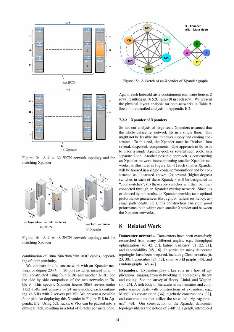
7.2.2 Xpander of Xpanders
So far, our analysis of large-scale Xpanders assumed thatthe whole datacenter network fits in a single floor. Thismight not be feasible due to power supply and cooling con-straints. To this end, the Xpander must be “broken” intoseveral, dispersed, components. One approach to do so isto place a single Xpander-pod, or several such pods, in aseparate floor. Another possible approach is constructingan Xpander network interconnecting smaller Xpander net-works, as illustrated in Figure 15: (1) each smaller Xpanderwill be housed in a single container/room/floor and be con-structed as illustrated above; (2) several (higher-degree)switches in each of these Xpanders will be designated as“core switches”; (3) these core switches will then be inter-connected through an Xpander overlay network. Since, asevidenced by our results, an Xpander provides near-optimalperformance guarantees (throughput, failure resiliency, av-erage path length, etc.), this construction can yield goodpeformance both within each smaller Xpander and betweenthe Xpander networks.
8 Related WorkDatacenter networks. Datacenters have been extensivelyresearched from many different angles, e.g., throughputoptimization [47, 42, 27], failure resiliency [31, 22, 21],and expandability [48, 16]. In particular, many datacentertopologies have been proposed, including Clos networks [6,23, 38], hypercubes [24, 52], small-world graphs [45], andrandom graphs [48, 47].
Expanders. Expanders play a key role in a host of ap-plications, ranging from networking to complexity theoryand coding. See the survey of Hoory, Linial, and Wigder-son [26]. A rich body of literature in mathematics and com-puter science deals with constructions of expanders, e.g.,Margulis’s construction [34], algebraic constructions [32],and constructions that utilize the so-called “zig-zag prod-uct” [43]. Our construction of the Xpander datacentertopology utilizes the notion of 2-lifting a graph, introduced
14

by Bilu and Linial [10, 33]. Utilizing expanders as networktopologies has been proposed in the context of parallel com-puting and high-performance computing [49, 15, 14, 9], op-tical networks [41] and also for peer-to-peer networks anddistributed computing [40, 39]. Our focus, in contrast, is ondatacenter networking and on tackling the challenges thatarise in this context (e.g., specific, throughput-related per-formance measures, specific routing and congestion controlprotocols, costs, incremental growth, etc.).
Relation to [50]. Our preliminary results on Xpander ap-peared at HotNets 2015 [50]. Here, we provide a deeper andmuch more detailed evaluation of the merits of expanderdatacenters in general, and of Xpander in particular, includ-ing (1) implementation and evaluation on the OCEAN SDNtestbed [3], (2) comparison of Xpander to Slim-Fly includ-ing theoretical results and simulations, (3) many additionalsimulation results with the MPTCP simulator for Xpanderand fat tree, (4) results for path-lengths, diameter and andincremental growth, (5) results for bisection bandwidth ofXpander, and (6) a detailed discussion of Xpander’s deploy-ment scenarios.
9 SummaryWe showed that expander datacenters offer many valuableadvantages over traditional datacenter designs and that thisclass of datacenters encompasses state-of-the-art propos-als for high-performance datacenter design. We suggestedpractical approaches for building such datacenters, namely,the Xpander datacenter architecture. We view Xpander asan appealing and practical alternative to traditional datacen-ter designs.
AcknowledgementsWe thank Nati Linial for many insightful conversationsabout expander constructions and Daniel Bienstock for hishelp in optimizing linear programs for throughput compu-tation. We thank Brighten Godfrey and Ankit Singla forsharing the Jellyfish code with us and for helpful discus-sions. We thank Soudeh Ghorbani for helping with run-ning experiments on the OCEAN platform. We thank NogaAlon, Alex Lubotzky, and Robert Krauthgamer for usefuldiscussions about expanders. We also thank Jonathan Perryfor suggesting Xpander’s color coding, presented in Sec-tion 7. Finally, we thank our shepherd, Siddhartha Sen, andthe anonymous CoNEXT reviewers, for their valuable feed-back. The 1st author is supperted by a Microsoft ResearchPh.D. Scholarship. The 2nd and 4th authors are supportedby the Israeli Center for Research Excellence (I-CORE) inAlgorithms. The 1st and 4th authors are supported by thePetaCloud industry-academia consortium. The third authoris supported in part by NSF awards 1464239 and 1535887.
References[1] IBM ILOG CPLEX Optimizer. http:
//www-01.ibm.com/software/commerce/
optimization/cplex-optimizer/index.html.
[2] MPTCP Simulator v0.2. http://nets.cs.pub.ro/˜costin/code.html.
[3] Ocean cluster for experimental architectures in net-works (ocean). http://ocean.cs.illinois.edu/.
[4] RipL-POX, simple datacenter controllerbuild on RipL. https://github.com/brandonheller/riplpox.
[5] Xpander Project Page. http://husant.github.io/Xpander.
[6] AL-FARES, M., LOUKISSAS, A., AND VAHDAT, A.A scalable, commodity data center network architec-ture. In SIGCOMM (2008).
[7] AL-FARES, M., RADHAKRISHNAN, S., RAGHAVAN,B., HUANG, N., AND VAHDAT, A. Hedera: Dynamicflow scheduling for data center networks. In NSDI(2010).
[8] AUMANN, Y., AND RABANI, Y. An O(log k) approx-imate min-cut max-flow theorem and approximationalgorithm. SIAM J. Comput. (1998).
[9] BESTA, M., AND HOEFLER, T. Slim Fly: A costeffective low-diameter network topology. In SC14(2014).
[10] BILU, Y., AND LINIAL, N. Lifts, discrepancy andnearly optimal spectral gap. Combinatorica (2006).
[11] BOLLOBAS, B. The isoperimetric number of randomregular graphs. Eur. J. Comb. (1988).
[12] C. PAASCH, S. BARRE, ET AL. Multipath TCP in theLinux Kernel. http://www.multipath-tcp.org.
[13] CERF, V. G., COWAN, D. D., MULLIN, R. C., ANDSTANTON, R. G. A lower bound on the average short-est path length in regular graphs. Networks (1974).
[14] CHONG, F. T., BREWER, E. A., LEIGHTON, F. T.,AND KNIGHT, T. F., J. Building a better butterfly:the multiplexed metabutterfly. In ISPAN (1994).
[15] CHONG, F. T., BREWER, E. A., LEIGHTON, F. T.,AND KNIGHT, T. F., J. Scalable expanders: Exploit-ing hierarchical random wiring. In Parallel ComputerRouting and Communication. 1994.
[16] CURTIS, A. R., KESHAV, S., AND LOPEZ-ORTIZ, A.Legup: using heterogeneity to reduce the cost of datacenter network upgrades. In CoNEXT (2010).
[17] DE QUEIROS VIEIRA MARTINS, E., AND PASCOAL,M. M. B. A new implementation of yen’s rankingloopless paths algorithm. 4OR (2003).
[18] DINITZ, M., SCHAPIRA, M., AND SHAHAF, G.Large Fixed-Diameter Graphs are Good Expanders.ArXiv e-prints (2016).
15

[19] FRIEDMAN, J. Relative expanders or weakly rela-tively ramanujan graphs. Duke Math. J. 118, 1 (052003), 19–35.
[20] FRIEDMAN, J. A Proof of Alon’s Second Eigen-value Conjecture and Related Problems. Memoirs ofthe American Mathematical Society. American Math-ematical Soc., 2008.
[21] GEORGE B. ADAMS, I., AND SIEGEL, H. J. Theextra stage cube: A fault-tolerant interconnectionnetwork for supersystems. IEEE Trans. Computers(1982).
[22] GILL, P., JAIN, N., AND NAGAPPAN, N. Un-derstanding network failures in data centers: mea-surement, analysis, and implications. In SIGCOMM(2011).
[23] GREENBERG, A. G., HAMILTON, J. R., JAIN, N.,KANDULA, S., KIM, C., LAHIRI, P., MALTZ, D. A.,PATEL, P., AND SENGUPTA, S. Vl2: a scalable andflexible data center network. In SIGCOMM (2009).
[24] GUO, C., LU, G., LI, D., WU, H., ZHANG, X., SHI,Y., TIAN, C., ZHANG, Y., AND LU, S. Bcube: ahigh performance, server-centric network architecturefor modular data centers. In SIGCOMM (2009).
[25] GUO, C., WU, H., TAN, K., SHI, L., ZHANG, Y.,AND LU, S. Dcell: a scalable and fault-tolerant net-work structure for data centers. In SIGCOMM (2008).
[26] HOORY, S., LINIAL, N., AND WIGDERSON, A. Ex-pander graphs and their applications. Bull. Amer.Math. Soc. (2006).
[27] JYOTHI, S. A., SINGLA, A., GODFREY, P. B., ANDKOLLA, A. Measuring throughput of data center net-work topologies. In SIGMETRICS (2014).
[28] KARYPIS, G., AND KUMAR, V. A fast and high qual-ity multilevel scheme for partitioning irregular graphs.SIAM J. Sci. Comput. (1998).
[29] LANTZ, B., HELLER, B., AND MCKEOWN, N. Anetwork in a laptop: Rapid prototyping for software-defined networks. In HOTNETS (2010).
[30] LINIAL, N., LONDON, E., AND RABINOVICH, Y.The geometry of graphs and some of its algorithmicapplications. Combinatorica (1995).
[31] LIU, V., HALPERIN, D., KRISHNAMURTHY, A.,AND ANDERSON, T. F10: A fault-tolerant engineerednetwork. In NSDI (2013).
[32] LUBOTZKY, A., PHILLIPS, R., AND SARNAK, P. Ra-manujan graphs. Combinatorica (1988).
[33] MARCUS, A., SPIELMAN, D. A., AND SRIVASTAVA,N. Interlacing families I: Bipartite ramanujan graphsof all degrees. In FOCS (2013).
[34] MARGULIS, G. A. Explicit constructions of ex-panders. Problemy Peredaci Informacii (1973).
[35] MCKAY, B. D., MILLER, M., AND IR, J. A noteon large graphs of diameter two and given maximumdegree. Journal of Combinatorial Theory, Series B(1998).
[36] MCKEOWN, N., ANDERSON, T., BALAKRISHNAN,H., PARULKAR, G., PETERSON, L., REXFORD, J.,SHENKER, S., AND TURNER, J. Openflow: En-abling innovation in campus networks. In SIGCOMM(2008).
[37] MUDIGONDA, J., YALAGANDULA, P., AL-FARES,M., AND MOGUL, J. C. Spain: Cots data-center eth-ernet for multipathing over arbitrary topologies. InNSDI (2010).
[38] MYSORE, R. N., PAMBORIS, A., FARRINGTON, N.,HUANG, N., MIRI, P., RADHAKRISHNAN, S., SUB-RAMANYA, V., AND VAHDAT, A. Portland: a scal-able fault-tolerant layer 2 data center network fabric.In SIGCOMM (2009).
[39] NAOR, M., AND WIEDER, U. Novel architectures forp2p applications: The continuous-discrete approach.In SPAA (2007).
[40] PANDURANGAN, G., ROBINSON, P., AND TREHAN,A. DEX: Self healing expanders. In SPAA (2014).
[41] PATURI, R., LU, D.-T., FORD, J. E., ESENER, S. C.,AND LEE, S. H. Parallel algorithms based on ex-pander graphs for optical computing. Appl. Opt.(1991).
[42] POPA, L., RATNASAMY, S., IANNACCONE, G., KR-ISHNAMURTHY, A., AND STOICA, I. A cost compar-ison of datacenter network architectures. In CoNEXT(2010).
[43] REINGOLD, O., VADHAN, S., AND WIGDERSON, A.Entropy waves, the zig-zag graph product, and newconstant-degree expanders and extractors. In FOCS(2000).
[44] ROSEN, E., VISWANATHAN, A., AND CALLON, R.Multiprotocol Label Switching Architecture. RFC3031, 2001.
[45] SHIN, J.-Y., WONG, B., AND SIRER, E. G. Small-world datacenters. In SoCC (2011).
[46] SINGH, A., ONG, J., AGARWAL, A., ANDER-SON, G., ARMISTEAD, A., BANNON, R., BOV-ING, S., DESAI, G., FELDERMAN, B., GERMANO,P., KANAGALA, A., PROVOST, J., SIMMONS, J.,TANDA, E., WANDERER, J., HOLZLE, U., STUART,S., AND VAHDAT, A. Jupiter rising: A decade of clostopologies and centralized control in google’s data-center network. In Proceedings of the 2015 ACM Con-ference on Special Interest Group on Data Communi-cation (2015), SIGCOMM ’15, ACM.
[47] SINGLA, A., GODFREY, P. B., AND KOLLA, A.High throughput data center topology design. In NSDI(2014).
16

[48] SINGLA, A., HONG, C.-Y., POPA, L., AND GOD-FREY, P. B. Jellyfish: Networking data centers ran-domly. In NSDI (2012).
[49] UPFAL, E. An o(log n) deterministic packet-routingscheme. J. ACM (1992).
[50] VALADARSKY, A., DINITZ, M., AND SCHAPIRA,M. Xpander: Unveiling the Secrets of High-Performance Datacenters. In HOTNETS (2015).
[51] WISCHIK, D., RAICIU, C., GREENHALGH, A., ANDHANDLEY, M. Design, implementation and evalua-tion of congestion control for multipath TCP. In NSDI(2011).
[52] WU, H., LU, G., LI, D., GUO, C., AND ZHANG,Y. Mdcube: a high performance network structurefor modular data center interconnection. In CoNEXT(2009).
[53] YEN, J. Y. Finding the k shortest loopless paths in anetwork. Management Science (1971).
[54] ZOLA, J., AND ALURU, S. Encyclopedia of ParallelComputing. Springer.
Appendix A Derandomizing LiftsRecall the notion of “2-lifting” a graph from [10] (from Sec-tion 2): A 2-lift of G is a graph obtained from G by (1)creating two vertices v1 and v2 for every vertex v in G; and(2) for every edge e = (u, v) in G, inserting two edges (amatching) between the two copies of u (namely, u1 and u2)and the two copies of v (namely, v1 and v2). The latter canbe done in one of two ways: connecting each ui to vi, whichwe will refer to as a “|| matching”, or connecting u1 to v2and u2 to v1, which we will refer to as a “X matching”.
Our heuristic creates a “criss-cross 2-lift” of G as fol-lows: enumerate the edges in G arbitrarily and then 2-liftG such that all edges with odd numbers correspond to ||matchings in the 2-lift and edges with even numbers corre-spond to X matchings. Let G denote the criss-cross 2-lift ofG. Intuitively, the heuristic then repeatedly checks if sub-stituting some ||matching with a X matching, or vice versa,can improve the edge expansion of the graph, and changesthe graph accordingly. This goes on until no such changecan improve edge expansion.
As computing the exact edge expansion of a given graphis NP-hard [30], our heuristic instead computes the spectralgap, which closely approximates edge expansion (see [26]for an explanation of spectral gap and its relation to edgeexpansion).
Observe that this heuristic can be extended to derandom-izing k-lifts for any constant k > 0 in a straightforwardmanner.
Appendix B Incremental ExpansionOur deterministic heuristic takes as input a graph G andnumber N and adds N nodes to G such that the addition
Algorithm 1: Deterministic 2-Lift HeuristicInput: Graph G = (V,E)G = (E, V )← a “criss-cross” 2-lift of GImproved← Truewhile Improved do
Improved← FalseG = (E, V )← Gfor e = (u, v) ∈ E do
if (u1, v1) ∈ E then// an ||matchingreplace the edges (u1, v1), (u2, v2) with(u1, v2), (u2, v1) in G
else// an X connectionreplace the edges (u1, v2), (u2, v1) with(v, u), (v′, u′) in G
GapOld← SpectralGap(G)GapNew← SpectralGap(G)if GapNew > GapOrg then
G← GImproved← True
Output G
of each node involves few wiring changes. Intuitively, withthe addition of each node our heuristic selects the d
2 worstlinks in terms of contribution to edge expansion, removesthem, and connects the new node to all nodes that are in-cident to the removed links. Unfortunately, as computingedge expansion is intractable, the spectral gap (see [26]) isused as a proxy for edge expansion.
Appendix C Optimizing LPs
We have used the standard maximum multi-commodityflow model for all of our simulations, with several optimiza-tions, the model is as follows:
For a given graph G = (V,E) with a capacity functionc : E → R+. There are K commodities each of which isdefined by the triplet Ki = (si, ti, di), where si, ti are thesource and destination vertices and di is the desired amountof data we would like to pass from si to di. We define foreach commodity Ki the variable f ie describing the amountof flow the commodity i sends on the edge e, and let the vec-tor f i hold these values. As there are multiple commoditiespresent we would like to enforce some sort of fairness, wedo that by demanding that each commodity could send anequal (maximal) fraction of it’s demand - we denote thatfraction as α. Let A be the node-arc incidence matrix of thegraph G defined as follows:
Av,e =
1 ∃u ∈ V s.t. e = (v, u)
−1 ∃u ∈ V s.t. e = (u, v)
0 else
and define for every commodity k the following vectorbk:
17

Algorithm 2: Incremental Expansion AlgorithmInput: Graph G = (V,E) and number (desired size)N ∈ N d← deg(G)T← |V |GapMap← while |V | < T +N do
Q← for e = (v1, v2) ∈ E do
E ← E\eLapMatrix← LaplacianMatrix(G)eGap← SmallestEigenV alue(LapMatrix)E ← E ∪ eGapMap[e] = eGap
Sort GapMap by value (highest to lowest)for e = (v1, v2) ∈ Keys(GapMap) do
if |Q| = d thenbreak
else if v1 /∈ Q and v2 /∈ Q thenQ← Q ∪ v1, v2E ← E\e
Add a new node v to VConnect v to the vertices in Q
Output G
bke =
dk ∃u ∈ V s.t. e = (sk, u)
−dk ∃u ∈ V s.t. e = (u, tk)
0 else
Now using the above notations we can write the problempresented above as the following LP:
maxα
s.t.
∀i ∈ [K]∑e∈E
Ai,e · f ie − α · bie = 0
∀e ∈ E∑i∈[K]
f ie ≤ c(e)
∀e ∈ E,∀i ∈ [K] 0 ≤ f ie
Even tough it is correct this form is far from being effi-cient as there could be many commodities sharing the samesource or destination, which are treated as a separate entity- for example in an all-to-all scenario there are |V |2 suchcommodities. We will now present a more compact and ef-ficient form allowing us to reduce the size of the commodi-ties to be linear in |V |.
Firstly we convert the LP to its dual form:
minβ
s.t.
∀i ∈ [K]∑e∈E
Ai,e · f ie − bie = 0
∀e ∈ E∑i∈[K]
f ie − β · c(e) ≤ 0
∀e ∈ E,∀i ∈ [K] 0 ≤ f ie
C.1 Optimizing All-to-All
Assuming there are K commodities of the form (si, ti, di),we look at the set of source vertices v1, v2, . . . , vK andwe aggregate it by source in the set AggComm =si|1 ≤ i ≤ F and we note that F ≤ K. We next definethe following function D : V × V → R+:
D(s, t) =
di (s, t, di) is a commodity
−di (t, s, di) is a commodity
0 else
And so the previous form could be written like so:
min γ
s.t.
∀s ∈ AggComm∑e∈E
As,e · fse =∑j
(s,tj ,dj)∈AggComm
dj
∀s ∈ AggComm, ∀v ∈ V \s∑e∈E
Av,e · f ie = D(v, s)
∀e ∈ E∑i∈[K]
f ie − γ · c(e) ≤ 0
∀e ∈ E,∀i ∈ [K] 0 ≤ f ie
We note that the actual flow fraction, α, is then given byα = 1
γ .
Appendix D Theoretical Guarantees
In section 4.1.2 we presented the following theorem, with-out proof - the proof can be found below.
Theorem D.1. For any d-regular graph G on n vertices,there exists a traffic matrix T and a d-regular graph G∗ onn vertices such that α(G∗, T ) ≥ Ω(logd n) · α(G,T ).
Proof. Let π : V → V be a random permutation. Let G∗
be the graph obtained by including an edge u, v if andonly if π−1(u), π−1(v) is an edge in G (i.e. G∗ is just arandom isomorphism ofG). Let T be the traffic matrix suchthat Tu,v = 1 if u, v ∈ E(G∗) and Tu,v = 0 otherwise.Then clearly α(G∗, T ) = 1, since the traffic demands areexactly the edges of G∗.
To analyze what happens inG, note that sinceG has max-imum degree d, the average distance between two nodesis Ω(logd n). So since π is a random permutation, theexpected distance in G between two nodes that are adja-cent in G∗ is also Ω(logd n). So by linearity of expec-tations, E
[∑u,v:Tu,v=1 distG(u, v)
]≥ Ω(dn logd n).
Thus we can fix some π where this is true, i.e. where∑u,v:Tu,v=1 distG(u, v) ≥ Ω(dn logd n). Then if we
send α(G,T ) units of flow for every traffic demand, thetotal capacity used up is at least Ω(α(G,T ) ·dn logd n). Onthe other hand, the total capacity in G is only |E| = dn/2.Thus α(G,T ) ≤ O(1/ logd n). Putting this together, weget that α(G,T ) ≤ O
(1
logd n
)· α(G∗, T ).
18

(a) 2FCN (b) FatTree
(c) Xpander
Figure C16: A sketch of a 2-FCN, 3-FCN and Xpander network topologies
Appendix E Deploying Xpanders
Throughout the physical analysis we assume a rack con-taining 52U, corresponding to the dimensions as in E17. Asketch of a Fat-Tree and 2-FCN networks can be found inFigure C16.
Figure E17: Server rack dimensions
E.1 Container Datacenters
In section 7.1 we examined an Xpander network vs. 2-FCNwith degrees 48 and 32. We gave a summarized results inTable 8, we provide additional results in Table E10 and Ta-ble E11
E.2 Xpanders vs. Fat-Trees
In Section 5 we identified, for each uniform fat-tree topolo-gies with even degree between 8 and 24, a more cost ef-fective expander datacenter. Table E12 presents the detailsregarding these topologies.
Cost Analysis In Section 7.2.1 we suggested a possible de-ployment for Fat-Tree and Xpander topologies, Table E13discusses the length of cables resulting from this analysis.We present a possible floor plan for both Xpander and Fat-Tree in figures Figure E18 and Figure E19 respectively.
Figure E18: A k = 30 Xpander floor plan
Figure E19: A k = 32 fat-tree floor plan
E.3 Xpander vs. Low-Diameter NetworksBelow are the simulations for Jellyfish, as described in sec-tion 6.
19
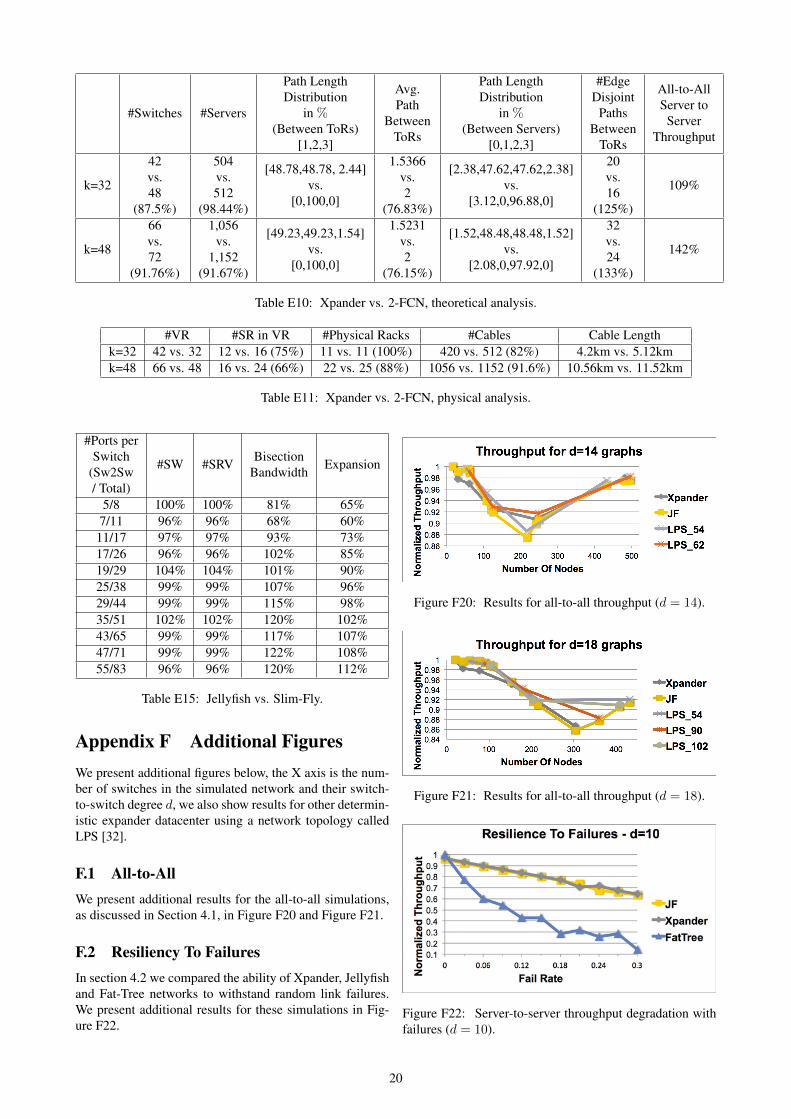
#Switches #Servers
Path LengthDistribution
in %(Between ToRs)
[1,2,3]
Avg.Path
BetweenToRs
Path LengthDistribution
in %(Between Servers)
[0,1,2,3]
#EdgeDisjoint
PathsBetween
ToRs
All-to-AllServer to
ServerThroughput
k=32
42vs.48
(87.5%)
504vs.512
(98.44%)
[48.78,48.78, 2.44]vs.
[0,100,0]
1.5366vs.2
(76.83%)
[2.38,47.62,47.62,2.38]vs.
[3.12,0,96.88,0]
20vs.16
(125%)
109%
k=48
66vs.72
(91.76%)
1,056vs.
1,152(91.67%)
[49.23,49.23,1.54]vs.
[0,100,0]
1.5231vs.2
(76.15%)
[1.52,48.48,48.48,1.52]vs.
[2.08,0,97.92,0]
32vs.24
(133%)
142%
Table E10: Xpander vs. 2-FCN, theoretical analysis.
#VR #SR in VR #Physical Racks #Cables Cable Lengthk=32 42 vs. 32 12 vs. 16 (75%) 11 vs. 11 (100%) 420 vs. 512 (82%) 4.2km vs. 5.12kmk=48 66 vs. 48 16 vs. 24 (66%) 22 vs. 25 (88%) 1056 vs. 1152 (91.6%) 10.56km vs. 11.52km
Table E11: Xpander vs. 2-FCN, physical analysis.
#Ports perSwitch
(Sw2Sw/ Total)
#SW #SRV BisectionBandwidth Expansion
5/8 100% 100% 81% 65%7/11 96% 96% 68% 60%
11/17 97% 97% 93% 73%17/26 96% 96% 102% 85%19/29 104% 104% 101% 90%25/38 99% 99% 107% 96%29/44 99% 99% 115% 98%35/51 102% 102% 120% 102%43/65 99% 99% 117% 107%47/71 99% 99% 122% 108%55/83 96% 96% 120% 112%
Table E15: Jellyfish vs. Slim-Fly.
Appendix F Additional FiguresWe present additional figures below, the X axis is the num-ber of switches in the simulated network and their switch-to-switch degree d, we also show results for other determin-istic expander datacenter using a network topology calledLPS [32].
F.1 All-to-AllWe present additional results for the all-to-all simulations,as discussed in Section 4.1, in Figure F20 and Figure F21.
F.2 Resiliency To FailuresIn section 4.2 we compared the ability of Xpander, Jellyfishand Fat-Tree networks to withstand random link failures.We present additional results for these simulations in Fig-ure F22.
Figure F20: Results for all-to-all throughput (d = 14).
Figure F21: Results for all-to-all throughput (d = 18).
Figure F22: Server-to-server throughput degradation withfailures (d = 10).
20

Fat-Treedegree
#Switches(#Servers)(Fat-Tree)
#Switches(#Servers)(Xpander)
#Portsusedfor
servers(Xpander)
#Portsusedfor
switches(Xpander)
#Portsused
(Xpander)
Server to Serverthroughput(Xpander)
Server to Serverthroughput(Fat-Tree)
8 80 (128) 64 (128) 2 6 8/8 9.786 · 10−3 8.065 · 10−3
10 125 (250) 125 (250) 2 8 10/10 6.435 · 10−3 4.082 · 10−3
12 180 (432) 144 (432) 3 8 11/12 2.428 · 10−3 2.347 · 10−3
14 245 (686) 237 (711) 3 10 13/14 1.805 · 10−3 1.473 · 10−3
16 320 (1024) 256 (1024) 4 12 16/16 1.177 · 10−3 9.84 · 10−4
18 405 (1458) 365 (1460) 4 12 16/18 9.51 · 10−4 6.9 · 10−4
20 500 (2000) 400 (2000) 5 15 20/20 5.98 · 10−4 5.03 · 10−4
22 605 (2662) 544 (2720) 5 16 21/22 4.58 · 10−4 3.77 · 10−4
24 720 (3456) 576 (3456) 6 17 23/24 3.22 · 10−4 2.9 · 10−4
Table E12: Xpanders vs. Fat-Trees, all-to-all analysis
5m 10m 15m 20m 25m 30m 35mFatTree 8,192 2,048 3,072 2,048 1,024 0 0Xpander 1,536 2,880 3,264 2,496 1,728 960 384
Table E13: Amount of cables used by k = 32 fat-tree vs. matching Xpander
SwitchDegree #Switches #Servers
Path LengthDistribution
in %(Between ToRs)
[1,2,3,4]
Avg.Path
BetweenToRs
Path LengthDistribution
in %(Between Servers)
[0,1,2,3,4]
#EdgeDisjoint
PathsBetween
Tors30vs.32
(93.75%)
1,152vs.
1,280(90%)
8,064vs.
8,192(98.44%)
[2,32.32,65.56,0.12]vs.
[0,2.9,97.1,0]
2.6379vs.
3.9413(66.93%)
[0.08,2,32.3,65.51,0.11]vs.
[0.19,0,2.93,0,96.88]
23vs.16
(143%)
Table E14: Xpander vs. fat-tree, theoretical analysis
21