Ximena Clark, joint with Alejandro MiccoMaritime Transport Costs and Port Efficiency

Maritime Transport Costs and Port Efficiency

This version: May 2001

By Ximena Clark, David Dollar, and Alejandro Micco1

1 World Bank; World Bank; and Inter-American Development Bank, respectively. Views expressed arethose of the authors and do not necessarily reflect official views of either the World Bank or the Inter-American Development Bank.

2

I. Introduction

Since the beginning of modern economics, the literature concerning the

determination of standards of living has also been interested in trade.2 Despite some

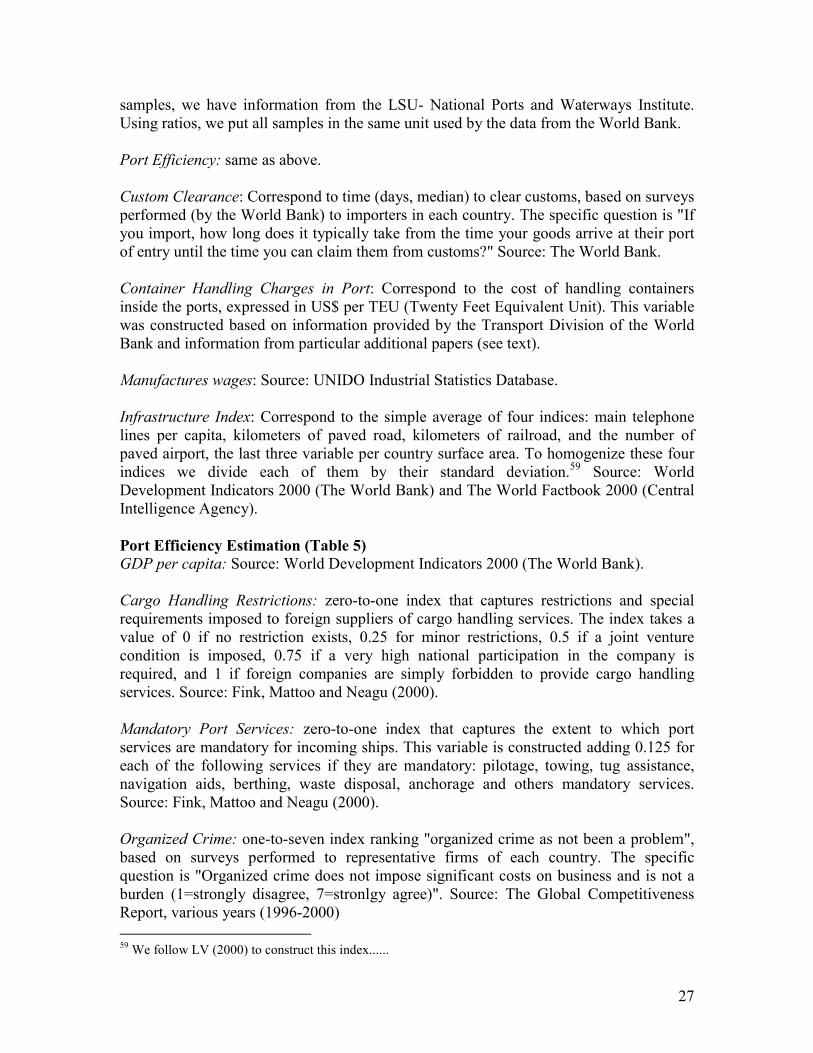
initial controversy, empirical studies show a positive relationship between trade and

growth. Frankel and Romer (1999) claim “…trade has a quantitatively large, significant,

and robust positive effect on income.”3

The lack of initial consensus among researchers on the relationship between trade

and growth has been mirrored by differences in the actual trade strategies of developing

countries. During the 1960s and into the 1970s, many countries adopted import

substitution policies to protect their infant industries, though a few economies in East

Asia took a different approach. By the 1990s many developing countries, including most

of the large ones, had shifted to an outward-oriented strategy and had seen accelerations

in their growth rates4.

These recent liberalizations have reduced tariff and, in some cases, non-tariff

barriers too. For instance, Latin America reduced its average tariff rate from almost 26%

at the beginning of the 1980s to 10% by the end of the 1990s and Asia reduced its

average tariff rate from 30% to 14%.5 These reductions in artificial trade barriers have

implied that the relative importance of transport costs as a determinant of trade has

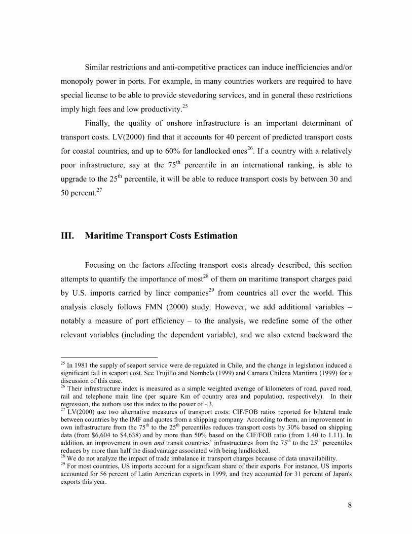
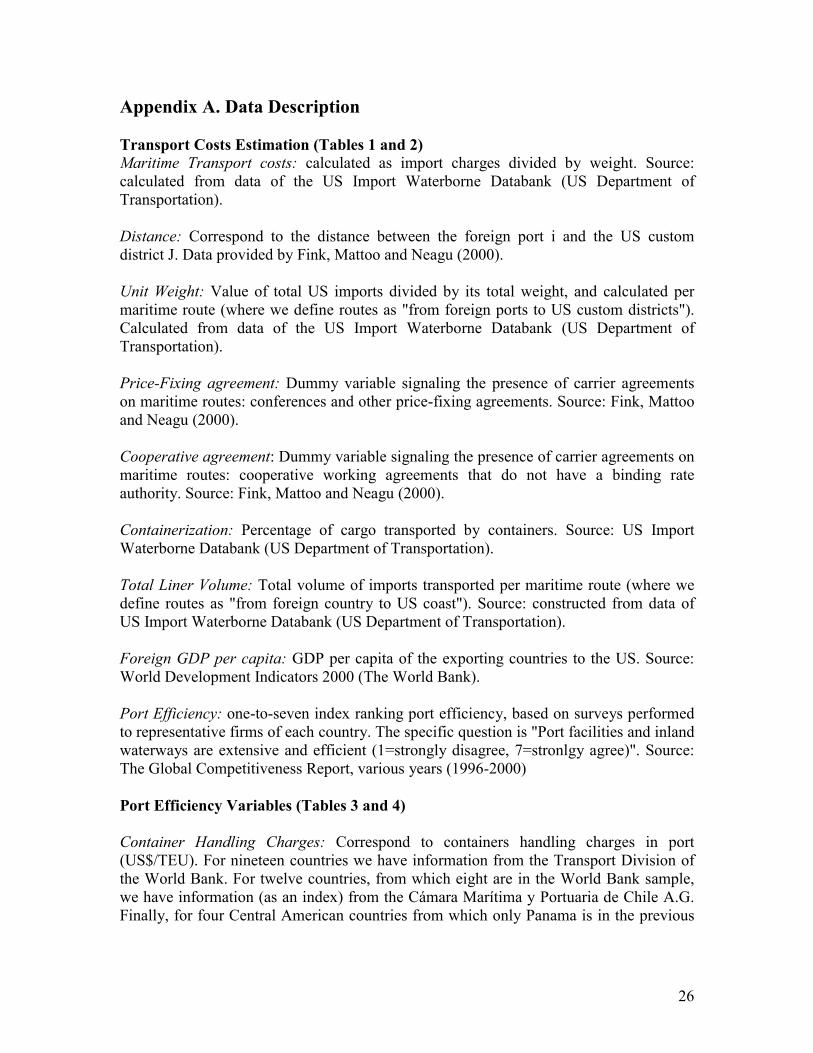
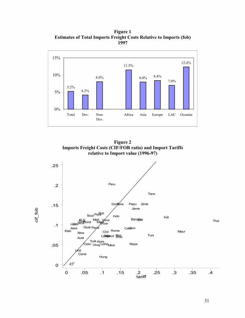
increased.6 As shown in Figure 1, total import freight costs represented 5.25 percent of

world imports (fob) in 1997. This percentage -which may seem low- is mainly driven by

developed countries, which represent more than 70 percent of world imports and whose

proximity to each other is reflected in a relatively low freight cost (4.2%). When

desaggregating these costs per region, they turn out to be substantially higher. Although

Latin America appears to have low freight costs relative to the other developing regions

2 Adams Smith (The Wealth of Nations, 1776), in his discussion of specialization and the extent of themarket stresses the relationship between wealth and trade between nations.3 Similarly, Ades and Glaeser (1999) find that openness accelerates growth of backward economies. For askeptical view of the cross-national evidence, see Rodriguez and Rodrik (1999).4 See Dollar and Kraay (2001).5 Central America and the Caribbean reduced its average tariff rate from 21% to 9% between these periods,and African countries from 30% to 20%. These average tariff rates correspond to simple averages acrosscountries of their unweighted tariff. If we consider weighted tariffs, the resulting average tariff rates by theend of the 90s should be smaller. (Source: World Bank)

3

(7% compared to 8% of Asia and 11.5% of Africa), the Latin American figure is

weighted by Mexico’s proximity to its main trading partner, the United States, and

consequently low freight costs. When Mexico is excluded, Latin American average

freight costs rise to 8.3 percent, more similar to the rest of the developing countries.

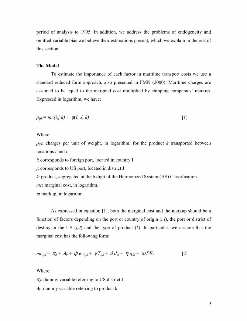
As liberalization continues to reduce artificial barriers, the effective rate of

protection provided by transport costs is now in many cases higher than the one provided

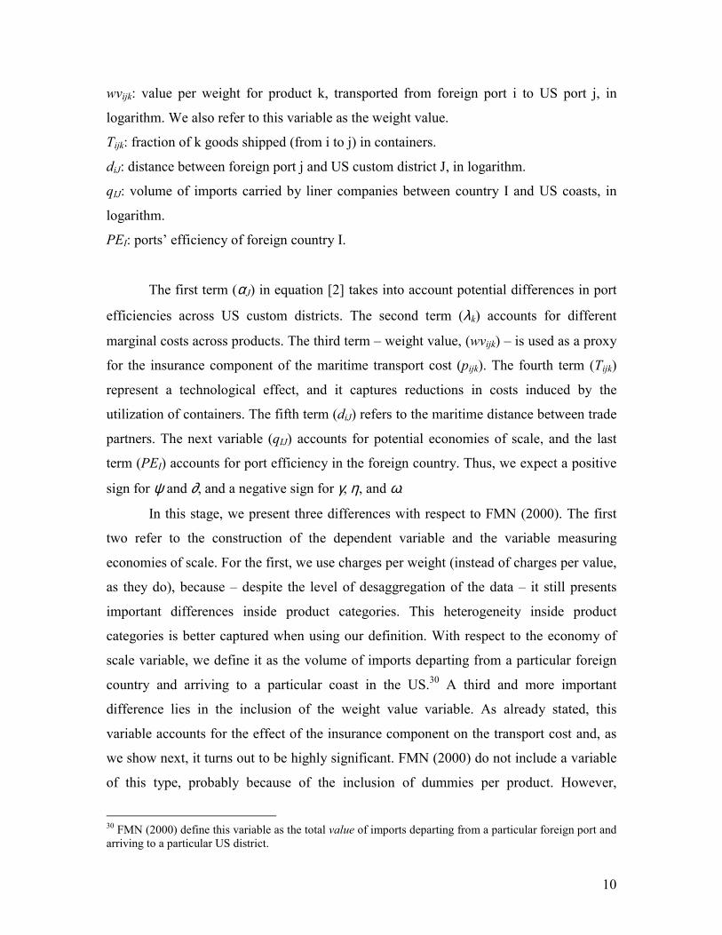
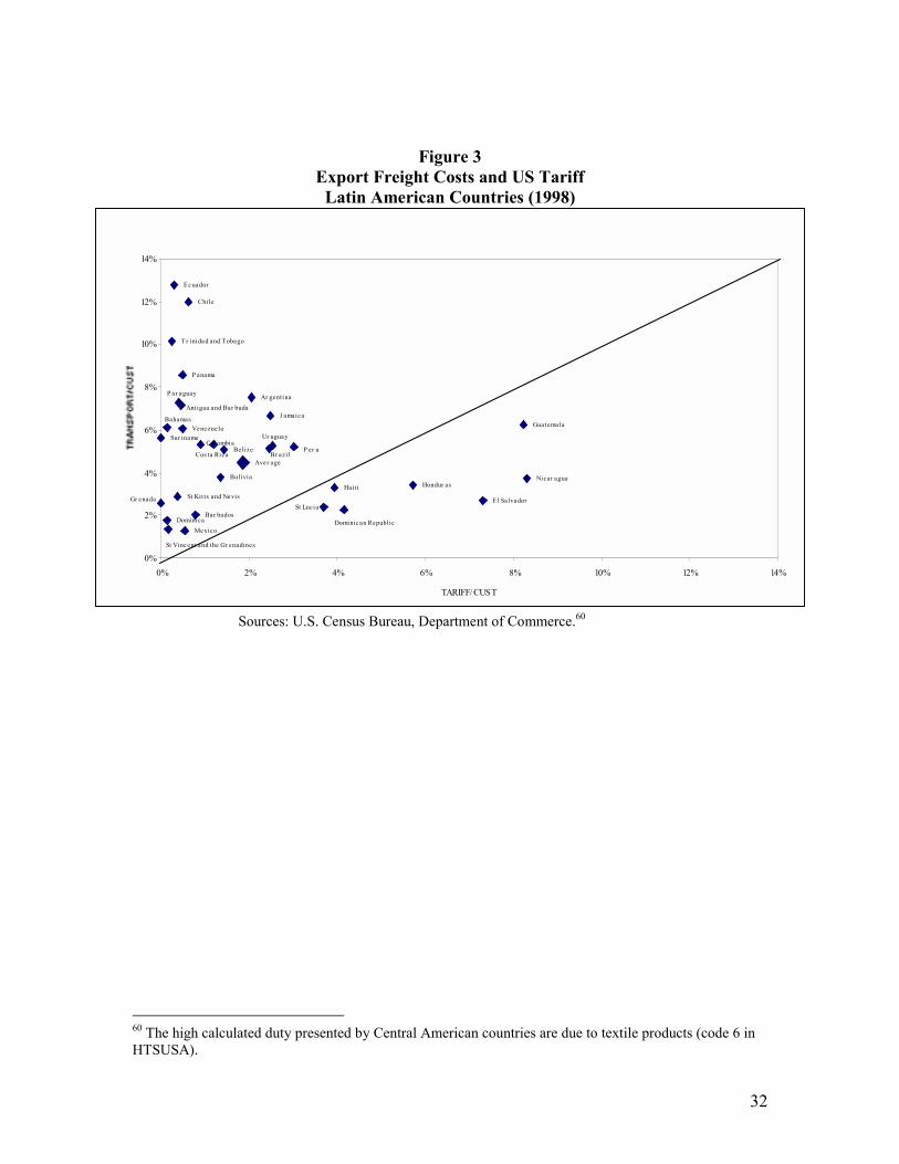
by tariffs. Figure 2 presents a comparison of average tariffs and a measure of transport

costs for various countries around the world, and Figure 3 presents an alternative

comparison of transport costs to the US and average tariffs faced in the US market by a

group of Latin American countries. From Figure 3, it is striking to realize that for some

countries, like Chile and Ecuador, transport costs exceed by more than twenty times the

average tariffs they face in the US market. Consequently, any additional effort to

integrate a country into the trading system should consider and analyze the effect of

transport costs and its determinants.

As a result, some immediate questions arise. How much do these transport costs

affect trade and growth? How much of these costs can be affected by government

policies? The broad literature that applies the gravity approach to the study of

international bilateral trade shows that geographical distance, which is used as proxy for

transport costs, is negatively related with trade.7 In a recent paper, Limao and Venables

(2000, henceforth LV) show that raising transport costs by 10 percent reduces trade

volumes by more than 20 percent. They also show that poor infrastructure accounts for

more than 40% of predicted transport costs. In a different analysis, Radelet and Sachs

(1998) show that shipping costs reduce the rate of growth of both manufactured exports

and GDP per capita. These authors claim that “… doubling the shipping cost (e.g. from an

8% to 16% CIF band) is associated with slower annual growth of slightly more than-half

of one percent point.”

In spite of the relevance of transport costs on trade and growth, shown by these

studies, there are not many other studies on transport costs. Moreover, these few studies

6 See Amjadi and Yeats (1995) and Radelet and Sachs (1998).7 An example of this literature is Bergstrand (1985).

4

rely on macro level data, which is certainly useful but misses the advantages that a

microdata can have. An exception is a recent study of Fink, Mattoo and Neagu (2000,

henceforth FMN), which analyzes the determinants of maritime transport costs in 1998,

focusing on the effect of non-competitive public and private policies. They find the latter

having a significant effect on transport costs. But, what about other factors influencing

transport costs, such as port efficiency? There is a wide consensus on the crucial

importance of port activities for the transport services. However, there are no measures of

how important are inefficiencies at port level for transport costs. This is one of the

objectives of this study. We analyze the effect of port efficiency on transport costs (in

addition to other standard variables), and then we explore the factors that lie behind port

efficiency.

Our analysis departs from FMN (2000) by incorporating port efficiency variables

and by redefining some variables. In addition, we address the problems of endogeneity

and omitted variable bias their estimations present, and we also extend backward the

period of analysis to 1995. We find that a 100 percent increase in distance raises maritime

transport costs by around 20 percent, a result that is quite consistent with the existent

literature. With respect to port efficiency, we find that improving port efficiency from the

25th to 75th percentiles reduces shipping costs by more than 12%. This result is robust to

different definitions of port efficiency as well as to different years.

In turn, when looking at the determinants of port efficiency, we find that the level

of infrastructure and organized crime exert a significant positive and negative influence

respectively. In addition, policy variables reflecting regulations at seaports affect port

efficiency in a non-linear way. This result suggests that having some level of regulation

increases port efficiency, but an excess of regulation could start to reverse these gains.

The remainder of this paper is structured as follows. Section II presents a

description of factors that may be behind transport costs. Section III describes the

econometric model used to quantify the relative importance of these factors affecting

transport costs. It also contains a description of the data used as well as the results of our

analyses. In Section IV, we analyze how important are infrastructure, regulation and

organized crime in explaining port efficiency. Section V concludes.

5

II. What Factors Explain Maritime Transport Costs?

As shown, transport costs may be an important barrier to trade and could have an

important effect on income. But why do some countries have higher transport costs than

others? What are the main determinants of these transport costs? Can government

policies affect these costs? Following some previous studies,8 this section addresses these

questions, based on a qualitative and quantitative description of transport cost

determinants. Given its relative importance (and also the availability of data), the main

focus in this paper is on international maritime transport cost.

The nature of services provided by shipping companies forces them to be

transnational companies serving more than one country. In general, these companies have

access to international capital markets and they are able to hire workers from all over the

world9, although under some restrictions sometimes. In any case, we should not expect

differences in capital or labor costs to be the main factors in explaining differences of

transport costs across countries. There are many other important specific factors affecting

transport costs across countries, which we present next.

The obvious and most studied determinant of transport cost is geography,

particularly distance10. The greater the distance between two markets, the higher the

expected transport cost for their trade. Using shipping company quotes for the cost of

transporting a standard container from Baltimore (USA) to selected worldwide

destinations, LV(2000) find that an extra 1,000 km raises transport costs by $380 (or 8%

for a median shipment). Moreover, breaking the journey into an overland and a sea

component, an extra 1,000 km by sea raises costs by only $190 while the same distance

by land raises costs by $1,380—4 and 30 percent of a median shipment, respectively. In

addition, if a country is landlocked, transport costs rise by $2,170, almost a 50 percent

8 This section follows McConville (1999) Fuchsluger (1999), Limao and Venables (2000), and Fink,Mattoo and Neagu (2000).9 Shipping companies prefer to sail their ships under open-registry flags. In fact, Panama, Liberia, Cyprusor Bahamas account for more than 40 percents of world fleet (measured in dead weight tons -dwt-) –UNCTAD (1998)-.10 It has long been recognizes that bilateral trade patterns are well described empirically by the so-calledgravity equation, which relates bilateral trade positively to both countries GDP and negatively to thedistance between them (which is used as proxy for transport cost). See Bergstrand (1985).

6

increase in the average cost.11 In other words, being landlocked is equivalent to being

located 10,000 km farther away from markets.

Trade composition additionally helps to explain transport costs differences across

countries. First of all, due to the insurance component of transport costs, products with

higher unit value have higher charges per unit of weight. On average, insurance fees are

around 2 percent of the traded value and they represent around 15 percent of total

maritime charges. Therefore, high value added exporting countries should have higher

charges per unit weight due to this insurance component. On the other hand, some

products require special transport features and therefore have different freight rates. 12

Directional imbalance in trade between countries implies that many carriers are

forced to haul empty containers back. As a result, either imports or exports become more

expensive. Fuchsluger (2000) shows that this phenomenon is observed in the bilateral

trade between the US and the Caribbean. In 1998, for instance, 72 percent of containers

sent from the Caribbean to the US were empty. This excess of supply in the northbound

route implied that a US exporter paid 83 percent more than a US importer for the same

type of merchandise between Miami and Port of Spain (Trinidad and Tobago).13 Similar

phenomenon occurs in the Asian-US and the Asian-European trade routes, where

westbound excess of supply means that Asian exporters end up paying more than 50% of

extra charge in transport costs than their eastbound counterparts (the US and Europe)14.

Maritime transport is a classic example of example of an industry that faces

increasing return to scale. Alfred Marshall put it clearly long ago: “… a ship’s carrying

power varies as the cube of her dimensions, while the resistance offered by the water

11 This result controls by the extra overland distance that must be overcome by landlocked countries toreach the sea.12 LSU-National Ports and Waterways Institute (1998) shows that the average freight rates between CentralAmerica and Miami for cooled load merchandise is about twice the transport cost for textiles.13 The actual freight rate for a 20-foot dry container between Port of Spain and Miami were $1,400 and$750 for the southbound and northbound route, respectively.14 Ships going from Asia to the US utilize more than 75 percent of their capacity, while when going back toAsia the utilization does not even attain a 50 percent rate. The rates from Asia to the US and in the oppositedirection are $1561/TEU and $999/TEU respectively. The capacity utilization of ships from Asia to Europeis 75% and 58% in the opposite direction, while the rates charged by shipping companies are $1353/TEUand $873/TEU respectively.

7

increase only a little faster than the square of her dimensions"15. Besides increasing

returns at the vessel level, there are economies of scale at the seaport level. For instance,

at the port of Buenos Aires (Argentina) the cost of using the access channel is $70 per

container for a 200 TEU16 vessel but only $14 per container for a 1000 TEU vessel. 17 In

general, even though most of these economies of scale are at the vessel level, in practice

they are related to the total volume of trade between two regions. Maritime routes with

low trade volume are covered by small vessel and vice versa. 18

In addition, the development of containerized transport has been an important

technological change in the transport sector during the last decades. Containers have

allowed large cost reductions in cargo handling, increasing cargo transshipment and

therefore national and international cabotage.19 In turn, this increase in cabotage has

induced the creation of hub ports that allow countries or regions to take advantage of

increasing return to scale.20

Commercial routes more liable to competition and less subject to monopoly

power will tend to have lower markups. Monopoly powers can be sustained either by

government restrictive trade policies or by private anti-competitive practices (cartels).

The former includes a variety of cargo reservation schemes, for example the UN Liner

Code.21 Private anti-competitive practices include, among others, the practice of fixing

rates of maritime conferences.22 Some authors have claimed that maritime conferences

have reduced their power in recent years,23 which has forced shipping companies to

merge as a way to hold their monopoly power.24

15 Quoted by McConville (1999). Additional economies of scale come from both material to build thevessel and labor to operate it (especially that of navigation).16 TEU is a standard container measure and it refers to Twenty Feet Equivalent Unit.17 See Fuchsluger (2000).18 See PIERS, On Board Review, Spring 1997.19 Cabotage refers to transshipment of the merchandise before it arrives to its final destination.20 See Hoffman (2000).21 This agreement stipulates that conference trade between two economies can allocate cargo according tothe 40:40:20 principle. Forty per cent of tonnage is reserved for the national flag lines of each exportingand importing economy and the remaining 20 per cent is to be allocated to liner ships from a thirdeconomy.22 Maritime conferences enjoy an exemption from competition rules in major trading countries, like the USand the European Union.23 In the last years there have been some reforms in the regulation affecting international shipping. Forinstance, the United States’ Ocean Shipping Reform Act of 1998 eroded the power of conferences, creatinggreater scope for price competition.24 See Fink, Mattoo and Neagu (2000) and Hoffman (2000).

8

Similar restrictions and anti-competitive practices can induce inefficiencies and/or

monopoly power in ports. For example, in many countries workers are required to have

special license to be able to provide stevedoring services, and in general these restrictions

imply high fees and low productivity.25

Finally, the quality of onshore infrastructure is an important determinant of

transport costs. LV(2000) find that it accounts for 40 percent of predicted transport costs

for coastal countries, and up to 60% for landlocked ones26. If a country with a relatively

poor infrastructure, say at the 75th percentile in an international ranking, is able to

upgrade to the 25th percentile, it will be able to reduce transport costs by between 30 and

50 percent.27

III. Maritime Transport Costs Estimation

Focusing on the factors affecting transport costs already described, this section

attempts to quantify the importance of most28 of them on maritime transport charges paid

by U.S. imports carried by liner companies29 from countries all over the world. This

analysis closely follows FMN (2000) study. However, we add additional variables –

notably a measure of port efficiency – to the analysis, we redefine some of the other

relevant variables (including the dependent variable), and we also extend backward the

25 In 1981 the supply of seaport service were de-regulated in Chile, and the change in legislation induced asignificant fall in seaport cost. See Trujillo and Nombela (1999) and Camara Chilena Maritima (1999) for adiscussion of this case.26 Their infrastructure index is measured as a simple weighted average of kilometers of road, paved road,rail and telephone main line (per square Km of country area and population, respectively). In theirregression, the authors use this index to the power of -.3.27 LV(2000) use two alternative measures of transport costs: CIF/FOB ratios reported for bilateral tradebetween countries by the IMF and quotes from a shipping company. According to them, an improvement inown infrastructure from the 75th to the 25th percentiles reduces transport costs by 30% based on shippingdata (from $6,604 to $4,638) and by more than 50% based on the CIF/FOB ratio (from 1.40 to 1.11). Inaddition, an improvement in own and transit countries’ infrastructures from the 75th to the 25th percentilesreduces by more than half the disadvantage associated with being landlocked.28 We do not analyze the impact of trade imbalance in transport charges because of data unavailability.29 For most countries, US imports account for a significant share of their exports. For instance, US importsaccounted for 56 percent of Latin American exports in 1999, and they accounted for 31 percent of Japan'sexports this year.

9

period of analysis to 1995. In addition, we address the problems of endogeneity and

omitted variable bias we believe their estimations present, which we explain in the rest of

this section.

The Model

To estimate the importance of each factor in maritime transport costs we use a

standard reduced form approach, also presented in FMN (2000). Maritime charges are

assumed to be equal to the marginal cost multiplied by shipping companies’ markup.

Expressed in logarithm, we have:

pijk = mc(i,j,k) + φ(I, J, k) [1]

Where:

pijk: charges per unit of weight, in logarithm, for the product k transported between

locations i and j.

i: corresponds to foreign port, located in country I

j: corresponds to US port, located in district J

k: product, aggregated at the 6 digit of the Harmonized System (HS) Classification

mc: marginal cost, in logarithm.

φ: markup, in logarithm.

As expressed in equation [1], both the marginal cost and the markup should be a

function of factors depending on the port or country of origin (i,I), the port or district of

destiny in the US (j,J) and the type of product (k). In particular, we assume that the

marginal cost has the following form:

mcijk = αJ + λk + ψ wvijk + γ Tijk + ∂ diJ + η qIJ + ω PEI [2]

Where:

αJ: dummy variable referring to US district J.

λk: dummy variable referring to product k.

10

wvijk: value per weight for product k, transported from foreign port i to US port j, in

logarithm. We also refer to this variable as the weight value.

Tijk: fraction of k goods shipped (from i to j) in containers.

diJ: distance between foreign port j and US custom district J, in logarithm.

qIJ: volume of imports carried by liner companies between country I and US coasts, in

logarithm.

PEI: ports’ efficiency of foreign country I.

The first term (αJ) in equation [2] takes into account potential differences in port

efficiencies across US custom districts. The second term (λk) accounts for different

marginal costs across products. The third term – weight value, (wvijk) – is used as a proxy

for the insurance component of the maritime transport cost (pijk). The fourth term (Tijk)

represent a technological effect, and it captures reductions in costs induced by the

utilization of containers. The fifth term (diJ) refers to the maritime distance between trade

partners. The next variable (qIJ) accounts for potential economies of scale, and the last

term (PEI) accounts for port efficiency in the foreign country. Thus, we expect a positive

sign for ψ and ∂, and a negative sign for γ, η, and ω.

In this stage, we present three differences with respect to FMN (2000). The first

two refer to the construction of the dependent variable and the variable measuring

economies of scale. For the first, we use charges per weight (instead of charges per value,

as they do), because – despite the level of desaggregation of the data – it still presents

important differences inside product categories. This heterogeneity inside product

categories is better captured when using our definition. With respect to the economy of

scale variable, we define it as the volume of imports departing from a particular foreign

country and arriving to a particular coast in the US.30 A third and more important

difference lies in the inclusion of the weight value variable. As already stated, this

variable accounts for the effect of the insurance component on the transport cost and, as

we show next, it turns out to be highly significant. FMN (2000) do not include a variable

of this type, probably because of the inclusion of dummies per product. However,

30 FMN (2000) define this variable as the total value of imports departing from a particular foreign port andarriving to a particular US district.

11

because of the insufficient level of desaggregation of the data, product dummies are not

enough and the exclusion of this variable can cause important omitted variable bias31.

Finally, and here we follow more closely FMN (2000) formulation, we assume

that shipping companies’ markups have the following form:

φ(I, J, k) = µk + ψPA AIJPA + ψCA AIJ

CA [3]

Where

AIJPA: existence of price-fixing agreements between country I and US district J.

AIJCA: existence of cooperative working agreement between country I and US district J.

The first term (µk) in the above equation reflects a product-specific effect that

captures differences in transport demand elasticity across goods (this is a derived demand

from the final demand of good k in the US). The last two terms account for potential

collusive agreements between shipping companies covering a same route. Two types of

agreements are distinguished: price-fixing agreements (which include most maritime

conferences), and cooperative working agreements that do not have binding rate setting

authority. Substituting the second and third equations on the first one, we obtain the

econometric model to be estimated:

pijk = αJ + βk + ψ wvijk + γ Tijk + ∂ diJ + ηqIJ + ω PEI + ψPAAIJPA + ψCAAIJ

CA + εijk

[4]

Where:

βk≡λ k +µ k

εijk: error term.

31 We replicated FMN (2000) estimations with and without the unit value variable (which is the relevantvariable to add in their specification, based on their construction of the dependent variable). The variableturned out to be highly significant (even after using product dummies), but their results for the rest of thevariables changed dramatically.

12

Data32 and Results

Data on maritime transport costs, value and volume of imports, and shipping

characteristics – like the percentage of the goods transported through containers – come

from the U.S. Import Waterborne Databank (U.S. Department of Transportation). Our

dependent variable – transport costs – is constructed using imports charges, defined by

the U.S. Census Bureau as: "...the aggregate cost of all freight, insurance, and other

charges (excluding U.S. import duties) incurred in bringing the merchandise from

alongside the carrier at the port of exportation -in the country of exportation- and placing

it alongside the carrier at the first port of entry in the United States.”

The U.S. Import Waterborne Databank covers the period 1995-1998. Even though

this database includes all U.S. imports carried by sea, classified by type of vessel service

(liner, tanker and tramp), we focus only on liner services to be able to estimate the effect

of conferences and agreements in maritime charges.33 Liner imports account for around

50 percent of total US imports and 65 percent of US maritime imports.34 Given that our

objective is to focus only on maritime transport costs, we also drop all the observations

for which the origin of the import is different from the port of shipment35.

The distance variable and the data on maritime conferences and working

agreement between liners were kindly provided by FMN(2000). The first correspond to

the distance between foreign ports and US custom districts, it is expressed in nautical

miles, and comes from a private service. The data on carrier agreements - used by FMN

to construct their indices- comes from the Federal Maritime Commission, it covers 59

countries and is available only for 1998. Therefore, when estimating for the other years

(1995-97), we have no choice but to use the same 1998 values for all the years.

Unfortunately, there is not much comparable information about port efficiency –at

port level- to be used in a cross-country analysis.36 So, we use an aggregated measure -

32 Appendix A gives a complete description of the data used.33 This also allow us to compare our results with FMN (2000) ones. Liner services are scheduled carriersthat advertise in publications advance of sailing. They generally have a fix itinerary and tend to carry mixedtypes of containerized, non-bulk cargo. Tramp and tanker services, in turn, are (dry, liquid) bulk carriersand have no regular scheduled itineraries, but are more depending on momentary demand.34 The remaining US imports by sea are carried by tramp services.35 That is, in transit merchandise is not included.36 The World Bank is launching a program (Global Facilitation Partnership for Transportation and Trade)to focus on significant improvements in the invisible infrastructure of transport and trade in different

13

per country- of port efficiency, consisting of a one-to-seven index (with 7 being the best

score) from the Global Competitiveness Report (GCR). This data covers the period 1995-

1999.37 As an alternative measure, we also use GDP per capita as a proxy for port

efficiency. Countries' GDP per capita are correlated with their level of infrastructure. For

our particular problem – explaining the cost of shipping the same product from different

ports in the world to the U.S. – it is hard to see why the per capita GDP of the sending

country would matter except to the extent that it is proxying for the quality of

infrastructure. As noted, we will use both this indirect measure and a direct measure of

port efficiency in different specifications.

In addition to the per capita GDP, we construct a second measure of infrastructure

– this time an index à la LV (2000) – for 1998, based on information at country level on

paved road, paved airports, railways and telephone lines38. We incorporate this variable

based on the assumption that the infrastructure level in a country is likely highly

correlated with the infrastructure level at their ports, and also because it allow us to

compare our results with LV (2000) ones. We should note that, despite having a

somewhat similar infrastructure index, our formulation differs from that of LV (2000) in

many respects. First, one of their measures of transport costs is the CIF/FOB ratio, which

has the disadvantage of being an aggregate measure for all products, while we use

transport cost information at product level. Also, this measure is well known for having

measurement deficiencies (although they try to control for that). Their second measure of

transport cost – shipping rates (for a homogeneous product) from Baltimore to a group of

different countries – try to address these problems. However, as the same authors point

out, the shipping rates from Baltimore are not necessarily representative -not even for the

rest of the US ports-. Our database, on the other hand, has information from many ports

around the world to different ports in the US.39 An advantage of their second measure,

member countries. However, the project is in its first stage and it does not cover all the countries of oursample yet.37 The report, however, is based on microdata from annual surveys at firm level, made to a representativegroup of enterprises in every country. The particular question for port efficiency is: "Port facilities andinland waterways are extensive and efficient. (1 = strongly disagree, 7 = strongly agree)". The number ofcountries covered has been growing over time (from 44 in the 1996 report to 56 in the 2000 one).38 See the Appendix for a description of its construction.39 In addition, we believe their sample is biased in favor of African countries. The bad infrastructure andport quality of African countries may be biasing upward the coefficient estimates they obtain.

14

however, is that it allow them to construct an estimate of inland transport cost, which is

not our purpose in this paper.

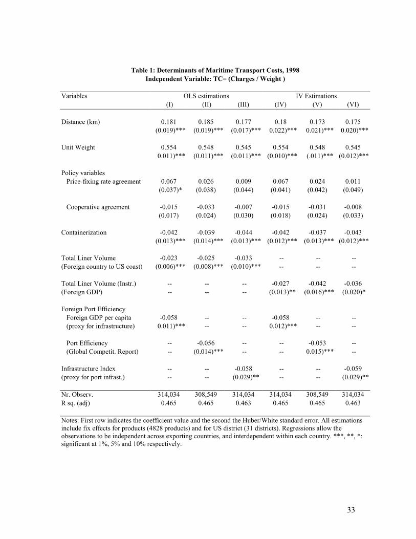
Table 1 reports our estimations for equation [4]. We start by presenting the results

only for 1998 because the variables on maritime conferences and working agreement

between liners refer to this particular year. The first three columns show the coefficients

using OLS, while the rest of the estimations use an Instrumental Variable (IV)

technique40. Columns I and IV report the results using GDP per capita as a proxy for port

efficiency, columns II and V use the variable port efficiency from the GCR, and columns

III and VI use the index of infrastructure we constructed. As it can be seen, in both type

of estimations most of the variables are highly significant and with the expected sign.

Distance has a significant (at 1%) positive effect on transport costs. A doubling in

distance, for instance, roughly generates a 20 percent increase in transport costs. This

distance elasticity close to .2 is consistent with the existent literature on transport costs.

The value per weight variable is also positive and highly significant, with a t-statistic

around 50. As already stated, these regressions include dummy variables for products at

the six-digit HS level. One might think that unit values would be quite similar across

countries at that level of disaggregation; not so. Feenstra (1996) shows that there is a

large variation in unit values even at the 10-digit HS level. He cites the examples of

men’s cotton shirts, which the U.S. imports from fully half of its 162 trading partners.

The unit values range from $56 (Japan) to $1 (Senegal). These differences in unit values

lead to large differences in insurance costs per kilogram, even for “homogeneous”

products. So, it is not surprising that we find that the more expensive the product, per unit

of weight, the higher the insurance and hence the overall transport cost.41

40 In all the estimations (OLS, IV), we allow the observations to be independent across exporting countries,but not necessarily independent within countries. At the same time, the standard errors presented in theTable correspond to the consistent Huber/White ones.41 In addition, there is the possibility that the unit weight variable could be capturing some measurementerrors. The argument is as follows. One should expect that the variables charges and (total) import valuewere very carefully measured, because the US custom constructs the dutiable value of imports by excludingthe former to the latter (and it should have a special interest in calculating it correctly). However, this couldnot be case for the measurement of weight. If so, measurement errors in the weight variable would induce apositive correlation between charges per weight (our dependent variable) and value per weight.

15

With respect to the two variables referring to agreements between liner

companies, only the first of them (price fixing binding agreements) turns out to be

positive -as expected- but only significant in one specification (at 10%).42 This result

seems to suggest that maritime conferences have been exerting some mild monopoly

power – adding an estimated 6.7% to transport costs in 1998, ceteris paribus. However, as

we will see later, this estimated effect of the price-fixing agreements is not significant for

other years.

The next variable, the level of containerization, presents a significant negative

effect on transport costs. As explained before, this variable represents technological

change at both vessels and seaport level. The idea behind this result is that

containerization reduces services cost, such as cargo handling, and therefore total

maritime charges.

The variable capturing economies of scale is the level of trade that goes through a

particular maritime route.43 This variable, calculated in terms of volume, has a significant

negative coefficient (as expected).44 However, the direct incorporation of this variable in

the estimations presents a problem of endogeneity (also presented in FMN (2000)). On

one hand, one should expect the bigger the trade the lower the transport costs. But, at the

same time, lower transport costs induce more trade. We address this problem in columns

IV to VI.

Finally, the coefficient related on port efficiency is negative and significant (at

1% in two cases and 5% in the other): the greater the efficiency at port level, the lower

the transport costs. This result is robust to the three alternative measures of port

efficiency (columns I, II and III). In particular, the coefficient for the measure from the

Global Competitiveness Report (column II), along with the distribution of the port

42 FMN (2000) find the price-fixing agreement dummy variable to be significant and much larger inmagnitude: between .4 and .51; that is, the maritime agreements add at least 40% to transport costs. Theyalso use policy variables referring to cargo reservation policies (not significant), cargo handling services(significant in one estimation but with wrong sign, and not significant in another), and mandatory portservices (significant, correct sign).43 Each couple foreign country and US coast is defined as a maritime route. We define three coast in theUS: East, West and Golf coast.44 We must note that this variable differs from the one presented by Fink, Mattoo and Neagu (2000) in twoaspects. First, they use the value of imports while we use the volume of imports (in tons). Second, thedefinitions of maritime route through which economies of scale arise are different: they use the trade (in

16

efficiency index among countries, indicates that an improvement in port efficiency from

the 25th to the 75th percentile reduces transport charges a little more than 12%.45 Similar

results are obtained for the other measures46.

To solve the endogeneity problem mentioned above, we use countries’ GDP as

instrument. We make the identifying assumption that if country size affects transport

costs, it does so through the volume of trade and economies of scale in shipping.

Columns IV to VI in Table 1 present the results for the instrumental variable (IV)

estimations. Most coefficients remain stable -with the expected signs- and they continue

to be significant, except for the price fixing agreement policy variable, which losses its

significance. Using the instrumental variables, the economy of scale variable remains

negative and significant, but the magnitude of the coefficient increases in absolute value

when we use the GCR measure of port efficiency (-0.042 v/s -0.025). Thus, we estimate

that doubling the volume of trade between a particular port and the U.S. reduces transport

costs by 3-4%. As we already mentioned, the coefficients for the rest of the variables -in

particular, for the three port efficiency measures- are quite stable.

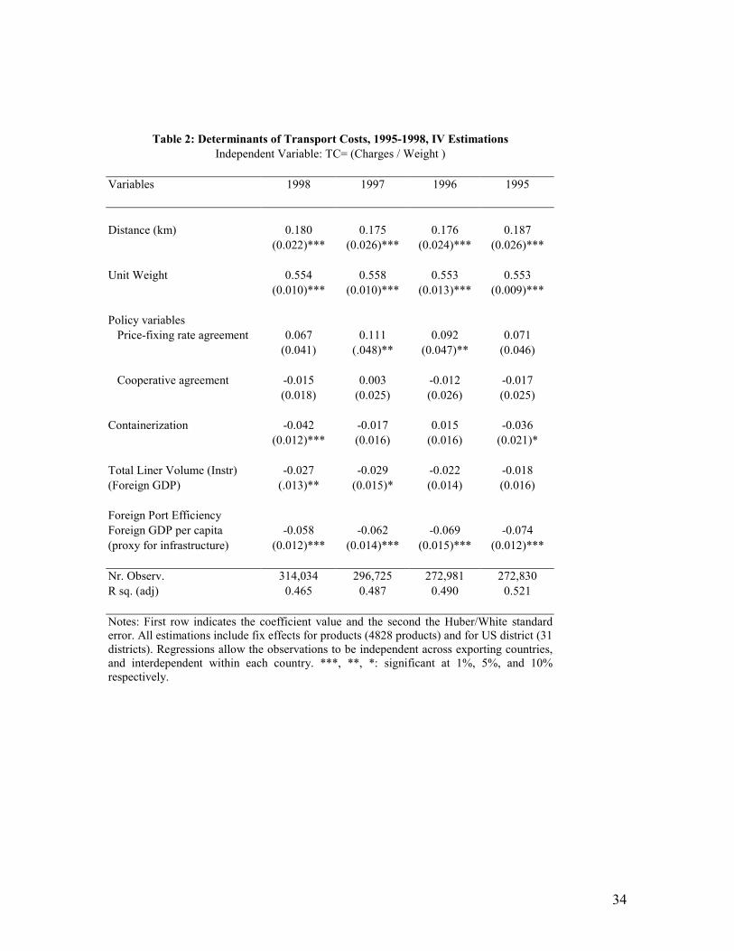
We performed similar estimations for the rest of the years for which we have data.

For brevity of space, Table 2 presents the estimated coefficients only for the IV

regressions using GDP per capita as a proxy for port efficiency.47

For each year, the coefficients on distance and weight value are quite stable and

significant (at 1%). Price-fixing rate agreement has the right sign in each year but it is

only significant in two years. Cooperative agreement, instead, is never significant. In

addition, when we use the port efficiency index from the GCR (not shown here) the

value) between foreign ports and US districts (31), while we use the trade (in volume) between foreigncountries and US coasts (3).45 That is, when port efficiency is measured with the GCR index, an improvement in port efficiency from25th to 75th percentile (i.e., from a score of 3.4 to 5.6 respectively) generates a maritime transport costsdecline of around 12%.46 When proxying port efficiency with the per capita GDP, an increase from the 25th to the 75th percentilereduces maritime transport charges in almost 15%. When using the infrastructure index, the reduction intransport cost is of 7%. This last variable could be showing a smaller effect because in fact it is measuringthe existence of infrastructure, but not necessarily its quality, while the other measures should capture alsoquality.47 The results with port efficiency from the GCR are similar. We do not report them because the number ofcountries for which we have data changes (sometimes considerably) over time.

17

price-fixing variable is only significant in 1997 (at 10%). From these results it is difficult

to conclude whether conferences have been exerting some monopoly power or not.

From Table 2 we can see that the coefficient on containerization is not stable over

time. It is significant only in 1998 and 1995. In the case of Total Liner Volumes, the

coefficient is only significant in the last two year (1997 and 1998). Finally, the estimated

coefficient for port efficiency is stable and significant from both an economic and

statistical point of view. When we used the port efficiency index from the GCR (not

shown here) we obtain similar results. These results allow us to conclude that port

efficiency is an important determinant of maritime transport costs. For example, if

countries like Ecuador, India or Brazil improved their port efficiency from their current

level to the 75th percentile -that is, to a level attained by France or Sweden- they would

reduce their maritime transport costs in more than 15% each.

A final caveat about these results. Our model assumes that, if inefficiency in a

port raises shipping costs by 10% for a shipment of shirts, it will increase the shipping

costs for a shipment of cars by the same 10%. Suppose, instead, that the “tax equivalent”

of port inefficiency varies by product. Then, products for which the tax is excessively

high will not be exported and we will not observe them in the data. In other words, we

have estimated the effect of port inefficiency for products that are actually shipped. The

effect may be higher for some products, which are then not exported. In this sense our

estimate of the cost of port inefficiency may be conservative.

IV. Determinants of Port Efficiency

The previous subsection stresses the importance of port efficiency on maritime

transport cost, but what are the factors behind port efficiency? The activities required at

port level are sometimes crucial for international trade transactions. These include not

only activities that depend on port infrastructure, like pilotage, towing and tug assistance,

or cargo handling (among others), but also activities related to customs requirements. It is

18

often claimed that "...the (in)efficiency, even timing, of many of port operations is

strongly influenced (if not dictated) by customs".48,49

Some legal restrictions can negatively affect port performance. For example, in

many countries workers are required to have special license to be able to provide

stevedoring services, artificially increasing seaport costs. Other deficiencies, associated

with port management itself, are also harmful to country competitiveness. For instance,

some ports still receive cargo without specifying the presentation of a Standard Shipping

Note, which is inconceivable in modern port practice. In many ports, it is quite

impossible to obtain a written and accurate account of the main port procedures, and

sometimes port regulations are not clear about the acceptance of responsibilities (for

cargo in shed or on the quay, for instance). All of this generates unreasonably long

delays, increases the risks of damage and pilferage of the products (in turn raising the

insurance premiums), and as a consequence considerably increases costs associated with

port activities.

Port efficiency varies widely from country to country and, specially, from region

to region. It is well know that some Asian countries (Singapore, Hong Kong) have the

most efficient ports in the world, while some of the most inefficient are located in Africa

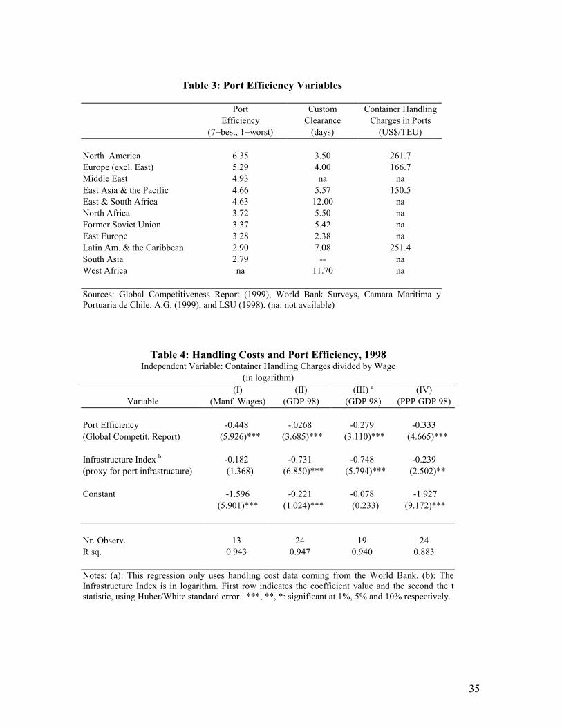
(Ethiopia, Nigeria, Malawi) or South America (Colombia, Venezuela, Ecuador). Table 3

presents some estimates of port efficiency, per geographic region50.

The first column is a subjective index based on surveys reported by the World

Economic Forum’s 1999 Global Competitiveness Report. North America and Europe

have the best rankings, followed by the Middle East, and East Asia & the Pacific. Latin

America and South Asia, in turn, are the regions perceived as having the least efficient

ports. The second column indicates the time, in median days, to clear customs (taken

from business surveys performed by the Inter-American Development Bank and World

48 Thus, any unexpected delay at ports due to extra custom requirements or cargo inspections, for instance,may increase considerably the associated port costs (due to moving containers and storage of frozenproducts, for example) and hence reduce exporters competitiveness.49 See John Raven (2000), for a description of relevant issues concerning trade and transport facilitation.50 We must note that these efficiency variables -per regions- are not directly comparable to each other,because the availability of countries is not the same for each of the variables. Thus, we should think ofthese as complement rather than substitute measures.

19

Bank51). The striking results are the ones for Africa -East and South Africa, and West

Africa- for which the median number of days to clear customs is 12. Among East and

South African countries, Ethiopia (30 days), Kenya, Tanzania and Uganda (14 days each)

are the countries with bigger delays in clearing customs; while Cameroon (20 days),

Nigeria (18 days) and Malawi (17 days) are the West African countries with the biggest

delays.52 The second region presenting big problems at custom levels is Latin America,

with a median delay in clearing customs of 7 days. In this group, Ecuador (15 days) and

Venezuela (11 days) appear as the worst performers.

Finally, the third column of Table 3 presents some estimates of the costs of

handling containers inside the ports (in US$/TEU). This variable was constructed based

on information provided by the Transport Division of the World Bank and information

from additional papers.53 Despite the fact that the sample of countries for this variable is a

lot more restricted than for the previous ones, the estimates are quite consistent with the

previous variables. While the efficient ports in East Asia present lower charges, the Latin

American ports have the most expensive handling services. This relationship is even

clearer when we take into account wage differential across countries. Table 4 presents the

regression of handling costs -adjusted by wage- on port efficiency and an index of

infrastructure (same as used in table 1). This index -at country level- is included under the

assumption that infrastructure at country level is highly correlated with infrastructure at

port level. In Column I handling costs are adjusted by manufacturing wages,54 in Column

II and III we adjust by per capita GDP (as proxy for wages), and in Column IV handling

cost is adjusted by PPP GDP per capita.

Port efficiency is an important determinant of handling cost. Countries with

inefficient seaports having higher handling costs. The negative and significant coefficient

on GDP per capita implies that countries with good infrastructure have lower seaport

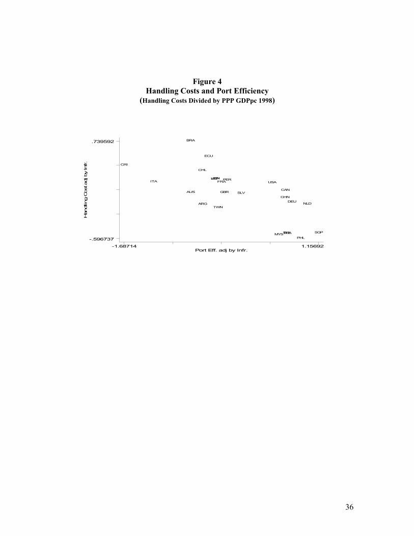
costs. Figure 4 presents the relationship between handling costs and port efficiency,

controlling for PPP GDP per capita (Column IV specification of Table 4). Countries

51 The specific question is: “If you import, how long does it typically take from the time your goods arriveat their port of entry until the time you can claim them from customs?”52 The African countries' results from this survey are totally consistent with the results presented by theAfrican Competitiveness Report 2000/2001 (World Economic Forum), which performed the same customclearance question (though the average time presented by the latter are slightly higher).53 Camara Maritima y Portuaria de Chile (1999) and LSU (1998).

20

where ports are considered the most efficient (e.g. Singapore and Belgium) are at the

same time the ones whose ports charge the least for their services (in comparable units).

As already noted, some Latin American countries (Brazil, Ecuador) are among the worst

ranked in term of their efficiency and also present the highest charges per services (after

controlling by the level of infrastructure).55

Finally, we try to explain which are the factors behind port efficiency. As we

already mentioned in the case of transport costs, it is reasonable to think that the

determinants of port efficiency will not only consist of infrastructure variables, but also

of management and/or policy variables. Therefore, besides a proxy for port

infrastructure56, we include among the explanatory variables two policy variables, one

referring to Cargo Handling Restrictions and the other to Mandatory Port Services. Both

variables are zero-to-one indices from FMN (2000). The first captures restrictions and

special requirements imposed on foreign suppliers of cargo handling services, where

foreign suppliers refer to local companies with foreign participation.57 The second

captures the extent to which port services are mandatory for incoming ships.58 Both

indices represent restrictions at port level that could limit competition, so we can expect a

negative relationship between them and port efficiency. However, due to some quality

and security considerations, we also have to consider that it may be beneficial to have a

certain level of regulation at the seaports. Thus, we also explore the possibilities of non-

linearities of the effect of each of these indices on port efficiency.

As we already mentioned, we consider the overall level of infrastructure, which

we assume to be positively correlated with a country's level of seaport infrastructure. We

expect the better the infrastructure the higher the probability of an efficient port; that is, a

54 Manufacturing wages are taken from UNIDO Industrial Statistics Database.55 A similar result is obtained when manufacturing wages (from the UNIDO Industrial Statistics Database)are used -instead of GDP per capita- to adjust handling costs. Appendix B presents the values used toconstruct these series.56 We use the index of country infrastructure we constructed as proxy for port infrastructure.57 The index takes a value of 0 if no restriction exists, 0.25 for minor restrictions, 0.5 if a joint venturecondition is imposed, 0.75 if a very high national participation in the company is required, and 1 if foreigncompanies are simply forbidden to provide cargo handling services.58 This variable is constructed adding .125 for each of the following services if they are mandatory:pilotage, towing, tug assistance, navigation aids, berthing, waste disposal, anchorage and others mandatoryservices.

21

positive coefficient for this variable. Finally, we also include a Crime Index, taken from

the Global Competitiveness Report, and consisting of a one-to seven index ranking how

severe is organized crime in a particular country (with 7 meaning "not a problem"). The

idea behind the inclusion of this variable is that organized crime constitutes a direct threat

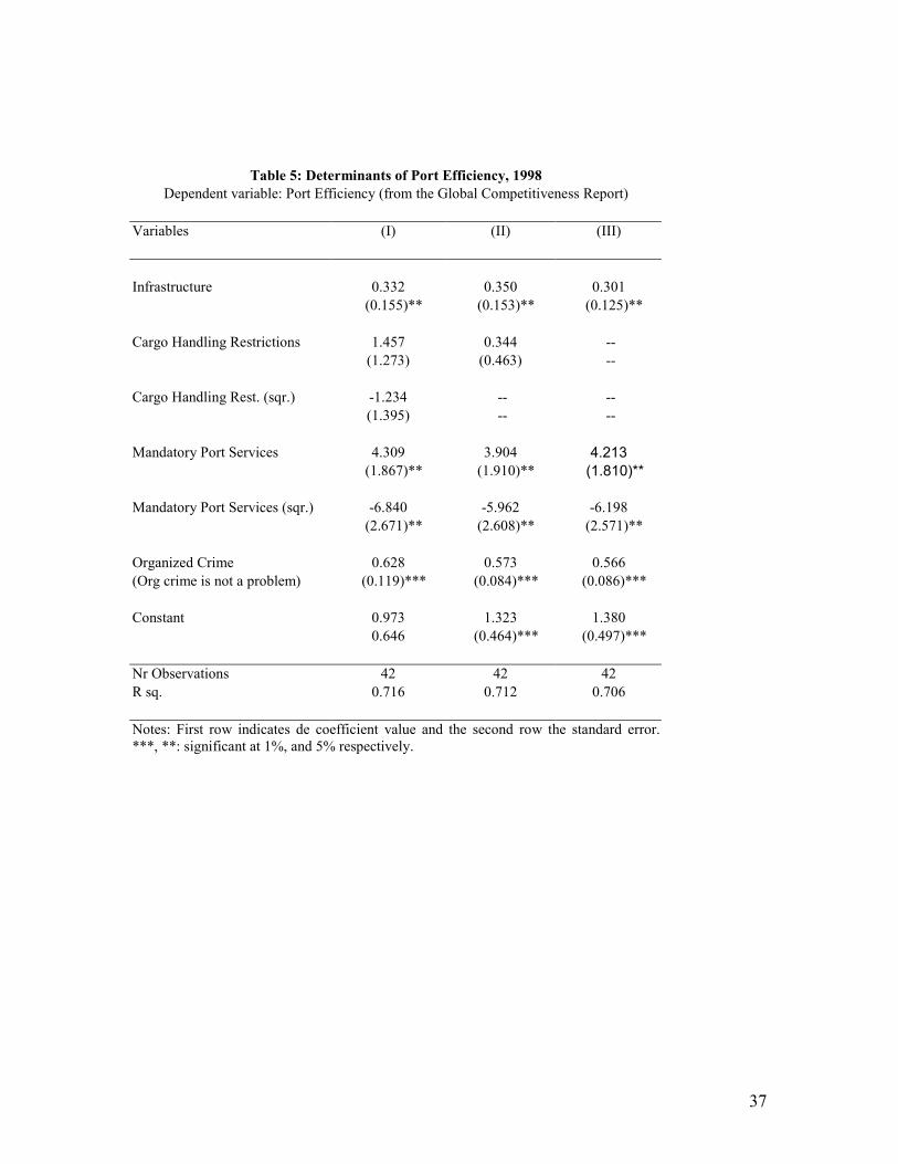
to port operations and merchandise in transit. With all of this in mind, we present in

Table 5 some estimations of the effects of these variables on port efficiency, calculated

for 1998.

As it can be seen, the coefficient on infrastructure is always positive and

significant. The results for the policy variables are somehow mixed, but make some

sense. Cargo handling restrictions are not significant, no matter the specification. The

variable for mandatory port services, on the other hand, is significant both in level and

square level, presenting a positive and negative sign, respectively. This result suggests

that having some level of regulations increases port efficiency, however, an excess of it

can start to reverse these gains. In terms of the countries in our sample, this result

suggests that Argentina is taking advantage of a moderate level of regulation in its

seaports, but instead Brazil is reducing its seaport efficiency because of excess regulation.

Finally, the crime variable also turns out to be highly significant and with the

expected positive sign (remember that the variable is defined as crime "not being a

problem"). In terms of this sample, an increase in organize crime from the 25th to 75th

percentile implies a reduction in port efficiency from the 50th to the 25th percentile.

V. Conclusion

By the 1990s many countries had adopted a development strategy emphasizing

integration with the global economy and therefore had reduced their tariff and non-tariff

barriers to trade. This reduction in artificial trade barriers has raised the importance of

transport costs as a remaining barrier to trade. Therefore, any strategy aimed at

integrating a country into the trading system has to take transport costs seriously.

Besides distance and other variables that no government can change, an important

determinant of maritime transport costs is seaport efficiency. An improvement in port

22

efficiency from 25th to 75th percentiles reduces shipping costs by more than 12%, or the

equivalent of 5,000 miles in distance. This result is robust to different definition of port

efficiency as well as to different years. Inefficient ports also increase handling costs.

Seaport efficiency, though, is not just a matter of physical infrastructure.

Organized crime has an important negative effect on port services, increasing transport

costs. In terms of our sample, an increase in organized crime from the 25th to 75th

percentile implies a reduction in port efficiency from 50th to 25th percentile. In addition

our results suggest that some level of regulation increases port efficiency, but excessive

regulation can be damaging.

23

References

Ades, A. and Glaeser, E. (1999). "Evidence on Growth, Increasing Return, and theExtend of the Market". Quarterly Journal of Economic. 114(3): 1025-1046.

Aghion,P., and Howitt, P. (1992).”A Model of Growth through Creative Destruction.”Econometrica 60:323-51.

Amjadi, A. and Yeats, A. J. (1995) "Have Transport Costs Contributed to the RelativeDecline of African Exports ?: Some Preliminary Empirical Evidence". Policy ResearchWorking Paper 1559, The World Bank, December.

Baird, A. (1999). “Privatization Defined; Is it the Universal Panacea”. Mimeo. NapierUniversity.

Bergstrand, J. (1985), “The Gravity Model in International Trade: Some MicroeconomicFoundations and Empirical Evidence”, Review of Economics and Statistics, 67:474-481.

Buenos Aires Port. (2000). http://www.buenosairesport.com.ar/anuari392.htm

Burkhalter, Larry. (1999). “Privatización portuaria: bases, alternativas y consecuencias”.Mimeo, ECLAC.

Cámara Marítima y Portuaria de Chile. A.G.. (1999). “Memoria annual No. 56”.

Cargo Systems – Latin American Supplement. (2000).Vol 27 No 10. London, U.K:Informa Business Publishing Ltd.

Dollar, D. and Kraay. A. (2001) "Trade, Growth and Poverty", The World Bank,Development Research Group, January, mimeo.

Estache, A. and Carbajo, J. (1996). “Competing Private Ports- Lessons from Argentina”Public Policy for the Private Sector. Note No. 100. World Bank Group.

ECLAC. (1998). “Modernización portuaria: una pirámide de deseafíos entrelazados”.Unidad de Transporte. Mimeo.

Foxley, J and Mardones, J.L. (2000). “Port Concessions in Chile”. Public Policy for thePrivate Sector. Note No. 223. World Bank Group

Frankel, J. and Romer, D. (1999). " Does Trade Cause Growth?". American EconomicReview (U.S.); 89:379-99, June.

Frink, C., Mattoo, A., and Neagu, I.C. (2000). ”Trade in International Maritime Servvice:How Much does Policy Matter? ” mimeo, World Bank.

24

Furchsluger (2000). "Port and Shipping Services in the Caribbean -the vital link forintegration-", mimeo.

Gaviria, J. (1998). “Port Privatization and Competition in Colombia”. Public Policy forthe Private Sector. Note No. 167. World Bank Group

Grossman, G.M., and Helpman, E. (1991a). Innovation and Growth in the GlobalEconomy. Cambridge, Mass.: MIT Press.

Grossman, G.M., and Helpman, E. (1991b). “Trade, Spillovers and Growth.“ EuropeanEconomic Review 35:517-526.

Hoffman, Jan. (2000) “El potencial de puertos pivotes en la costa del Pacíficosudamericano” Transport Unit, ECLAC. ECLAC Magazine, 71.

Hoffman, Jan. (1999a). “Las privatizaciones portuarias en América Latina en los 90:Determinantes y Resultados”. Transport Unit, ECLAC. Presented in Seminar of WorldBank held at Las Palmas, Spain.

Hoffman, Jan. (1999b). “After the Latin American ports privatization: The Emergence ofa ‘Latin American Model’”. Presented to the Fourth PdI World Port PrivatizationConference. London, September 1999. ECLAC.http://docs.vircomnet.com/mobility/seacargohandling_vd/pdi1.htm

Juhel, M. (1998). “Globalization, Privatization and Restructuring of Ports” World BankGroup. Document presented at the 10th Annual Australasian Summit.

Limao, N., and Venables, A.J. (2000).”Infratructure, Geographical Disadvantage andTransport Costs”. mimeo

LSU- National Ports and Waterways Institute. (1998) “Estudio de fletes para favorecer elcomercio exterior de Centroamérica”. Informe Final. Presentado a la ComisiónCentroamericana de Transporte Marítimo - COCATRAM

Nombela, G and Trujillo, L. (1999). “Privatization and Regulation of the SeaportIndustry”. Universidad de Las Palmas de Gran Canaria (Spain). Mimeo.

Radelet, S., and Sachs, J. (1998). ”Shipping Costs, Manufactured Exports and EconomicGrowth." mimeo Harvard Instituted for International Development.

Rivera-Batiz,L., and Romer,P.M. (1991). “Economic Integration and EndogenousGrowth.” Quarterly Journal of Economics 106(2):5331-555.

Rodriguez, F. and Rodrik, D. (1999).” Trade Policy and Economic Growth: A Skeptic’sGuide to the Cross-National Evidence.” NBER Working Paper No 7081.

25

Romer,P.M. (1990).”Endogeneous Technological Change.” Journal of Political Economy98(5) part 2:71-102.

Frankel, J.A., and Romer, D. “Does Trade Cause Growth.” The American EconomicReview, 89(3): 379-399.

Segerstrom, P. (1991) ”Innovation, Imitation and Economic Growth.” Journal ofPolitical Economy 99(4):807-827.

Sommer, D. (1999). “Private Participation in Port Facilities- Recent Trends” PublicPolicy for the Private Sector. Note No. 193. World Bank Group

The Global Competitiveness Report (various issues, 1996-2000), Harvard University(Cambridge, USA) and World Economic Forum (Geneva, Switzerland).

The African Competitiveness Report 2000/2001, Center for International Development atHarvard University (Cambridge, USA) and World Economic Forum (Geneva,Switzerland).

Trujillo, L. and Nombela, G. (1999) "Privatization and Regulation of the SeaportIndustry", Policy Research Working Paper 2181, The World Bank, September.

UNCTAD secretariat. (1999). “Review of Maritime Transport 1999”. United Nations,New York and Geneva.

Ventura, J. (1997). “ Growth and Interdependence.” Quarterly Journal of Economics112(1):57-84.

Viloria, J. (2000). “De Colpuertos a las Sociedades Portuarias: los Puertos del CaribeColombiano, 1990-1999” Document presented at II Simposio sobre la Economía de laCosta Caribe. Cartagena: Colombia.

Young, A. (1991).”Learning by Doing and the Dynamic Effects of International Trade.”Quarterly Journal of Economics 106(2): 369-406.

26

Appendix A. Data Description

Transport Costs Estimation (Tables 1 and 2)Maritime Transport costs: calculated as import charges divided by weight. Source:calculated from data of the US Import Waterborne Databank (US Department ofTransportation).

Distance: Correspond to the distance between the foreign port i and the US customdistrict J. Data provided by Fink, Mattoo and Neagu (2000).

Unit Weight: Value of total US imports divided by its total weight, and calculated permaritime route (where we define routes as "from foreign ports to US custom districts").Calculated from data of the US Import Waterborne Databank (US Department ofTransportation).

Price-Fixing agreement: Dummy variable signaling the presence of carrier agreementson maritime routes: conferences and other price-fixing agreements. Source: Fink, Mattooand Neagu (2000).

Cooperative agreement: Dummy variable signaling the presence of carrier agreements onmaritime routes: cooperative working agreements that do not have a binding rateauthority. Source: Fink, Mattoo and Neagu (2000).

Containerization: Percentage of cargo transported by containers. Source: US ImportWaterborne Databank (US Department of Transportation).

Total Liner Volume: Total volume of imports transported per maritime route (where wedefine routes as "from foreign country to US coast"). Source: constructed from data ofUS Import Waterborne Databank (US Department of Transportation).

Foreign GDP per capita: GDP per capita of the exporting countries to the US. Source:World Development Indicators 2000 (The World Bank).

Port Efficiency: one-to-seven index ranking port efficiency, based on surveys performedto representative firms of each country. The specific question is "Port facilities and inlandwaterways are extensive and efficient (1=strongly disagree, 7=stronlgy agree)". Source:The Global Competitiveness Report, various years (1996-2000)

Port Efficiency Variables (Tables 3 and 4)

Container Handling Charges: Correspond to containers handling charges in port(US$/TEU). For nineteen countries we have information from the Transport Division ofthe World Bank. For twelve countries, from which eight are in the World Bank sample,we have information (as an index) from the Cámara Marítima y Portuaria de Chile A.G.Finally, for four Central American countries from which only Panama is in the previous

27

samples, we have information from the LSU- National Ports and Waterways Institute.Using ratios, we put all samples in the same unit used by the data from the World Bank.

Port Efficiency: same as above.

Custom Clearance: Correspond to time (days, median) to clear customs, based on surveysperformed (by the World Bank) to importers in each country. The specific question is "Ifyou import, how long does it typically take from the time your goods arrive at their portof entry until the time you can claim them from customs?" Source: The World Bank.

Container Handling Charges in Port: Correspond to the cost of handling containersinside the ports, expressed in US$ per TEU (Twenty Feet Equivalent Unit). This variablewas constructed based on information provided by the Transport Division of the WorldBank and information from particular additional papers (see text).

Manufactures wages: Source: UNIDO Industrial Statistics Database.

Infrastructure Index: Correspond to the simple average of four indices: main telephonelines per capita, kilometers of paved road, kilometers of railroad, and the number ofpaved airport, the last three variable per country surface area. To homogenize these fourindices we divide each of them by their standard deviation.59 Source: WorldDevelopment Indicators 2000 (The World Bank) and The World Factbook 2000 (CentralIntelligence Agency).

Port Efficiency Estimation (Table 5)GDP per capita: Source: World Development Indicators 2000 (The World Bank).

Cargo Handling Restrictions: zero-to-one index that captures restrictions and specialrequirements imposed to foreign suppliers of cargo handling services. The index takes avalue of 0 if no restriction exists, 0.25 for minor restrictions, 0.5 if a joint venturecondition is imposed, 0.75 if a very high national participation in the company isrequired, and 1 if foreign companies are simply forbidden to provide cargo handlingservices. Source: Fink, Mattoo and Neagu (2000).

Mandatory Port Services: zero-to-one index that captures the extent to which portservices are mandatory for incoming ships. This variable is constructed adding 0.125 foreach of the following services if they are mandatory: pilotage, towing, tug assistance,navigation aids, berthing, waste disposal, anchorage and others mandatory services.Source: Fink, Mattoo and Neagu (2000).

Organized Crime: one-to-seven index ranking "organized crime as not been a problem",based on surveys performed to representative firms of each country. The specificquestion is "Organized crime does not impose significant costs on business and is not aburden (1=strongly disagree, 7=stronlgy agree)". Source: The Global CompetitivenessReport, various years (1996-2000) 59 We follow LV (2000) to construct this index......

28

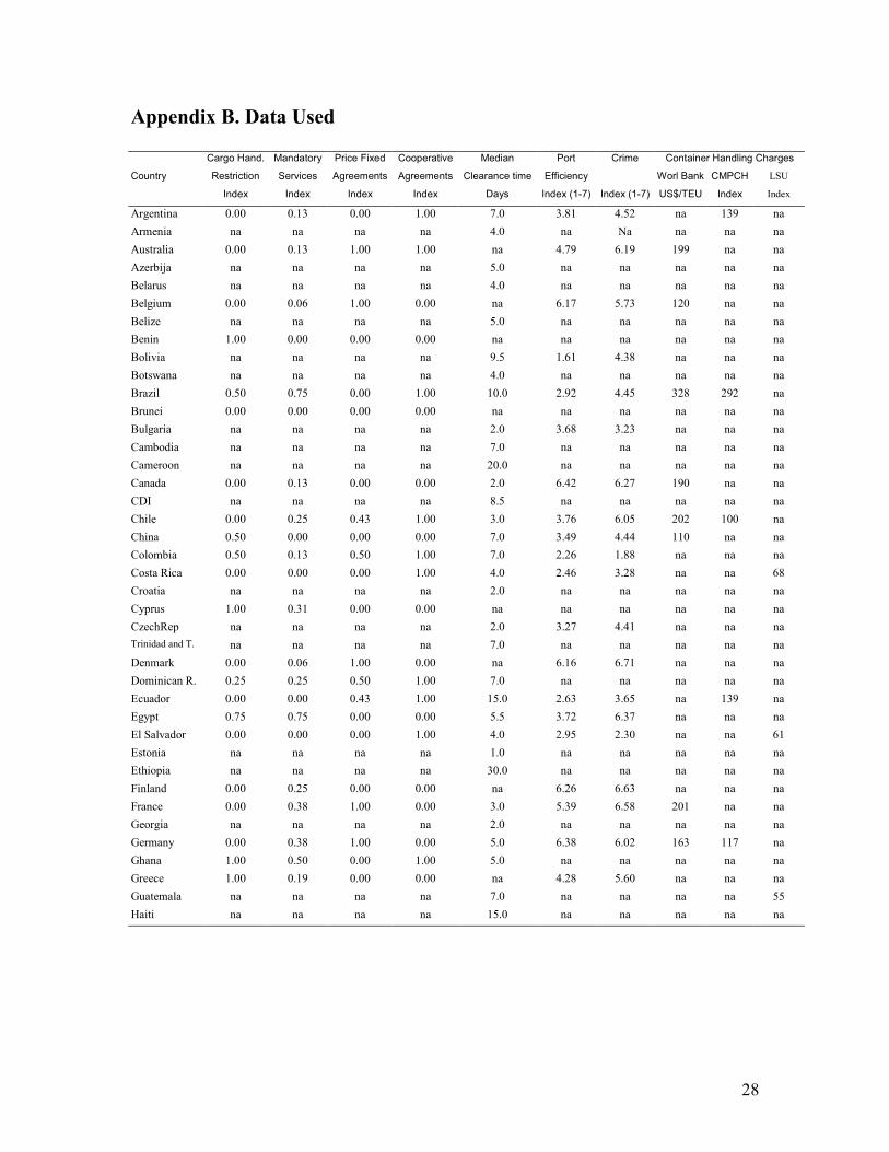
Appendix B. Data Used

Cargo Hand. Mandatory Price Fixed Cooperative Median Port Crime Container Handling Charges

Country Restriction Services Agreements Agreements Clearance time Efficiency Worl Bank CMPCH LSU

Index Index Index Index Days Index (1-7) Index (1-7) US$/TEU Index Index

Argentina 0.00 0.13 0.00 1.00 7.0 3.81 4.52 na 139 naArmenia na na na na 4.0 na Na na na naAustralia 0.00 0.13 1.00 1.00 na 4.79 6.19 199 na naAzerbija na na na na 5.0 na na na na naBelarus na na na na 4.0 na na na na naBelgium 0.00 0.06 1.00 0.00 na 6.17 5.73 120 na naBelize na na na na 5.0 na na na na naBenin 1.00 0.00 0.00 0.00 na na na na na naBolivia na na na na 9.5 1.61 4.38 na na naBotswana na na na na 4.0 na na na na naBrazil 0.50 0.75 0.00 1.00 10.0 2.92 4.45 328 292 naBrunei 0.00 0.00 0.00 0.00 na na na na na naBulgaria na na na na 2.0 3.68 3.23 na na naCambodia na na na na 7.0 na na na na naCameroon na na na na 20.0 na na na na naCanada 0.00 0.13 0.00 0.00 2.0 6.42 6.27 190 na naCDI na na na na 8.5 na na na na naChile 0.00 0.25 0.43 1.00 3.0 3.76 6.05 202 100 naChina 0.50 0.00 0.00 0.00 7.0 3.49 4.44 110 na naColombia 0.50 0.13 0.50 1.00 7.0 2.26 1.88 na na naCosta Rica 0.00 0.00 0.00 1.00 4.0 2.46 3.28 na na 68Croatia na na na na 2.0 na na na na naCyprus 1.00 0.31 0.00 0.00 na na na na na naCzechRep na na na na 2.0 3.27 4.41 na na naTrinidad and T. na na na na 7.0 na na na na naDenmark 0.00 0.06 1.00 0.00 na 6.16 6.71 na na naDominican R. 0.25 0.25 0.50 1.00 7.0 na na na na naEcuador 0.00 0.00 0.43 1.00 15.0 2.63 3.65 na 139 naEgypt 0.75 0.75 0.00 0.00 5.5 3.72 6.37 na na naEl Salvador 0.00 0.00 0.00 1.00 4.0 2.95 2.30 na na 61Estonia na na na na 1.0 na na na na naEthiopia na na na na 30.0 na na na na naFinland 0.00 0.25 0.00 0.00 na 6.26 6.63 na na naFrance 0.00 0.38 1.00 0.00 3.0 5.39 6.58 201 na naGeorgia na na na na 2.0 na na na na naGermany 0.00 0.38 1.00 0.00 5.0 6.38 6.02 163 117 naGhana 1.00 0.50 0.00 1.00 5.0 na na na na naGreece 1.00 0.19 0.00 0.00 na 4.28 5.60 na na naGuatemala na na na na 7.0 na na na na 55Haiti na na na na 15.0 na na na na na

29

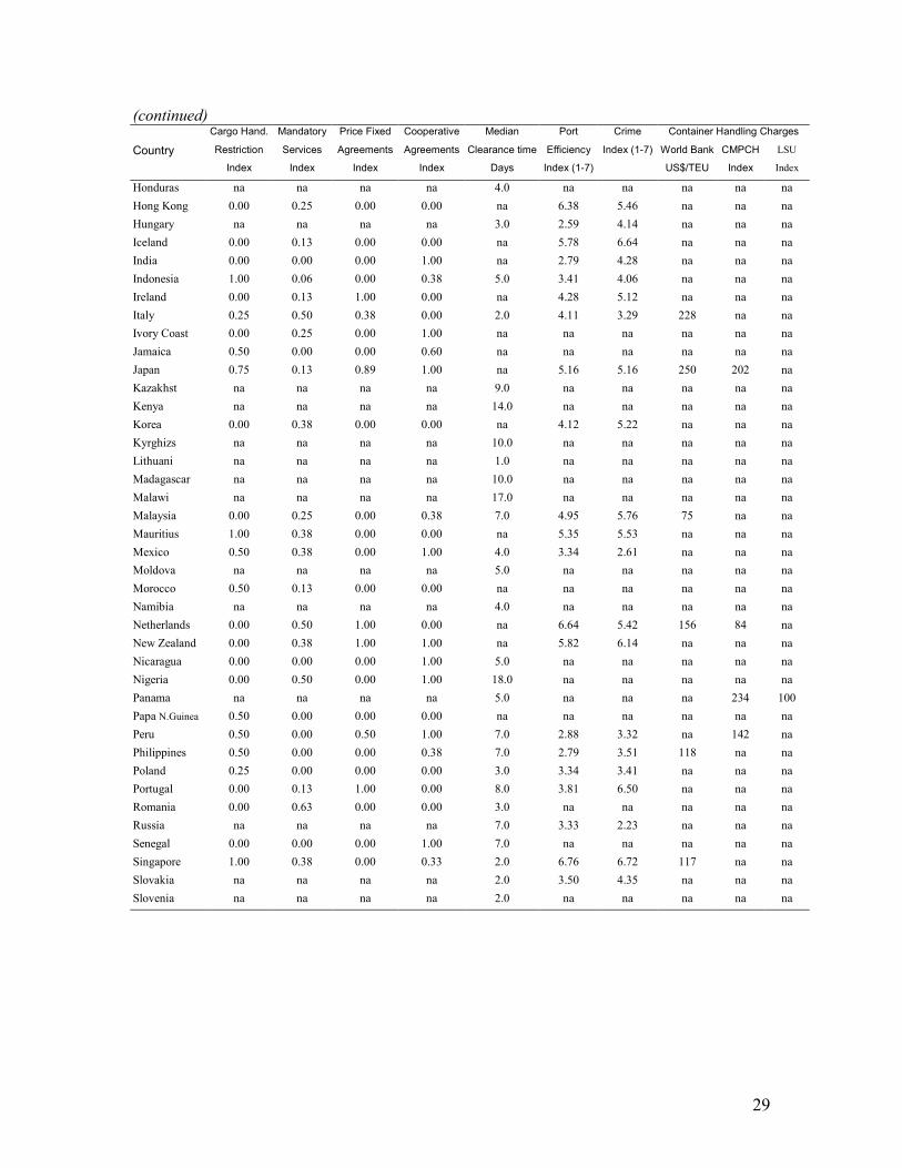
(continued)Cargo Hand. Mandatory Price Fixed Cooperative Median Port Crime Container Handling Charges

Country Restriction Services Agreements Agreements Clearance time Efficiency Index (1-7) World Bank CMPCH LSU

Index Index Index Index Days Index (1-7) US$/TEU Index Index

Honduras na na na na 4.0 na na na na naHong Kong 0.00 0.25 0.00 0.00 na 6.38 5.46 na na naHungary na na na na 3.0 2.59 4.14 na na naIceland 0.00 0.13 0.00 0.00 na 5.78 6.64 na na naIndia 0.00 0.00 0.00 1.00 na 2.79 4.28 na na naIndonesia 1.00 0.06 0.00 0.38 5.0 3.41 4.06 na na naIreland 0.00 0.13 1.00 0.00 na 4.28 5.12 na na naItaly 0.25 0.50 0.38 0.00 2.0 4.11 3.29 228 na naIvory Coast 0.00 0.25 0.00 1.00 na na na na na naJamaica 0.50 0.00 0.00 0.60 na na na na na naJapan 0.75 0.13 0.89 1.00 na 5.16 5.16 250 202 naKazakhst na na na na 9.0 na na na na naKenya na na na na 14.0 na na na na naKorea 0.00 0.38 0.00 0.00 na 4.12 5.22 na na naKyrghizs na na na na 10.0 na na na na naLithuani na na na na 1.0 na na na na naMadagascar na na na na 10.0 na na na na naMalawi na na na na 17.0 na na na na naMalaysia 0.00 0.25 0.00 0.38 7.0 4.95 5.76 75 na naMauritius 1.00 0.38 0.00 0.00 na 5.35 5.53 na na naMexico 0.50 0.38 0.00 1.00 4.0 3.34 2.61 na na naMoldova na na na na 5.0 na na na na naMorocco 0.50 0.13 0.00 0.00 na na na na na naNamibia na na na na 4.0 na na na na naNetherlands 0.00 0.50 1.00 0.00 na 6.64 5.42 156 84 naNew Zealand 0.00 0.38 1.00 1.00 na 5.82 6.14 na na naNicaragua 0.00 0.00 0.00 1.00 5.0 na na na na naNigeria 0.00 0.50 0.00 1.00 18.0 na na na na naPanama na na na na 5.0 na na na 234 100Papa N.Guinea 0.50 0.00 0.00 0.00 na na na na na naPeru 0.50 0.00 0.50 1.00 7.0 2.88 3.32 na 142 naPhilippines 0.50 0.00 0.00 0.38 7.0 2.79 3.51 118 na naPoland 0.25 0.00 0.00 0.00 3.0 3.34 3.41 na na naPortugal 0.00 0.13 1.00 0.00 8.0 3.81 6.50 na na naRomania 0.00 0.63 0.00 0.00 3.0 na na na na naRussia na na na na 7.0 3.33 2.23 na na naSenegal 0.00 0.00 0.00 1.00 7.0 na na na na naSingapore 1.00 0.38 0.00 0.33 2.0 6.76 6.72 117 na naSlovakia na na na na 2.0 3.50 4.35 na na naSlovenia na na na na 2.0 na na na na na

30

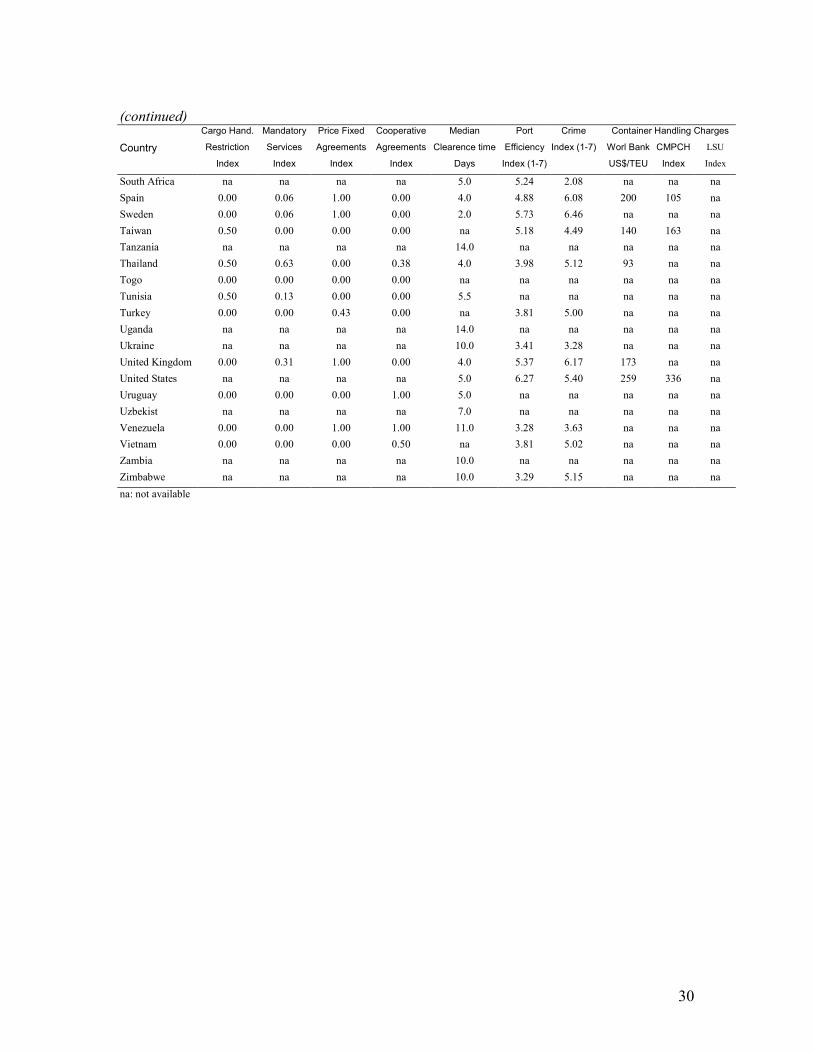
(continued)Cargo Hand. Mandatory Price Fixed Cooperative Median Port Crime Container Handling Charges

Country Restriction Services Agreements Agreements Clearence time Efficiency Index (1-7) Worl Bank CMPCH LSU

Index Index Index Index Days Index (1-7) US$/TEU Index Index

South Africa na na na na 5.0 5.24 2.08 na na naSpain 0.00 0.06 1.00 0.00 4.0 4.88 6.08 200 105 naSweden 0.00 0.06 1.00 0.00 2.0 5.73 6.46 na na naTaiwan 0.50 0.00 0.00 0.00 na 5.18 4.49 140 163 naTanzania na na na na 14.0 na na na na naThailand 0.50 0.63 0.00 0.38 4.0 3.98 5.12 93 na naTogo 0.00 0.00 0.00 0.00 na na na na na naTunisia 0.50 0.13 0.00 0.00 5.5 na na na na naTurkey 0.00 0.00 0.43 0.00 na 3.81 5.00 na na naUganda na na na na 14.0 na na na na naUkraine na na na na 10.0 3.41 3.28 na na naUnited Kingdom 0.00 0.31 1.00 0.00 4.0 5.37 6.17 173 na naUnited States na na na na 5.0 6.27 5.40 259 336 naUruguay 0.00 0.00 0.00 1.00 5.0 na na na na naUzbekist na na na na 7.0 na na na na naVenezuela 0.00 0.00 1.00 1.00 11.0 3.28 3.63 na na naVietnam 0.00 0.00 0.00 0.50 na 3.81 5.02 na na naZambia na na na na 10.0 na na na na naZimbabwe na na na na 10.0 3.29 5.15 na na nana: not available

31

Figure 1Estimates of Total Imports Freight Costs Relative to Imports (fob)

1997

Figure 2Imports Freight Costs (CIF/FOB ratio) and Import Tariffs

relative to Import value (1996-97)

5.2%4.2%

8.0%

11.5%

8.0% 8.4%7.0%

12.4%

0%

5%

10%

15%

Total Dev. Non-Dev.

Africa Asia Europe LAC Oceania

cif_

fob

tariff0 .05 .1 .15 .2 .25 .3 .35 .4

0

.05

.1

.15

.2

.25

ArgeAust

Bang

Boli

Braz

Cana

CentChil

Chin

Colo

Cost

Czec

Domi

EcuaEl S

EstoGuat

Hond

Hung

IndiIndo

Jama

Japa

Kore

Latv

Leba

LithMala

Malt

Maur

Mexi Nepa

New

NicaPana

Papu

Para

Peru

Phil

Pola

Roma

Saud

SoutSri

Tanz

ThaiTrin

Tuni

Turk

Unit

Urug

Vene

Zimb

45o

32

Figure 3Export Freight Costs and US Tariff

Latin American Countries (1998)

Sources: U.S. Census Bureau, Department of Commerce.60

60 The high calculated duty presented by Central American countries are due to textile products (code 6 inHTSUSA).

Aver age

Ar gentina

Ur uguay

P ar aguay

Br azi l

Chi le

Bolivia

P er u

Ecuador

Sur inameVenezue la

Colombia

Tr inidad and Tobago

Bar bados

Gr enada

St Vincent and the Gr enadines

St Lucia

Dominica

Antigua and Bar buda

St Kit ts and Nevis

Dominican Republ ic

Haiti

J amaicaBahamas

P anama

Cos ta Rica

Nicar aguaHondur as

El Salvador

Bel ize

Guatemala

Mexico

0%

2%

4%

6%

8%

10%

12%

14%

0% 2% 4% 6% 8% 10% 12% 14%

TARIFF/ CUST

33

Table 1: Determinants of Maritime Transport Costs, 1998Independent Variable: TC= (Charges / Weight )

Variables OLS estimations IV Estimations (I) (II) (III) (IV) (V) (VI)

Distance (km) 0.181 0.185 0.177 0.18 0.173 0.175 (0.019)*** (0.019)*** (0.017)*** 0.022)*** 0.021)*** 0.020)***

Unit Weight 0.554 0.548 0.545 0.554 0.548 0.545 0.011)*** (0.011)*** (0.011)*** (0.010)*** (.011)*** (0.012)***

Policy variables Price-fixing rate agreement 0.067 0.026 0.009 0.067 0.024 0.011

(0.037)* (0.038) (0.044) (0.041) (0.042) (0.049)

Cooperative agreement -0.015 -0.033 -0.007 -0.015 -0.031 -0.008(0.017) (0.024) (0.030) (0.018) (0.024) (0.033)

Containerization -0.042 -0.039 -0.044 -0.042 -0.037 -0.043 (0.013)*** (0.014)*** (0.013)*** (0.012)*** (0.013)*** (0.012)***

Total Liner Volume -0.023 -0.025 -0.033 -- -- --(Foreign country to US coast) (0.006)*** (0.008)*** (0.010)*** -- -- --

Total Liner Volume (Instr.) -- -- -- -0.027 -0.042 -0.036(Foreign GDP) -- -- -- (0.013)** (0.016)*** (0.020)*

Foreign Port Efficiency Foreign GDP per capita -0.058 -- -- -0.058 -- -- (proxy for infrastructure) 0.011)*** -- -- 0.012)*** -- --

Port Efficiency -- -0.056 -- -- -0.053 -- (Global Competit. Report) -- (0.014)*** -- -- 0.015)*** --

Infrastructure Index -- -- -0.058 -- -- -0.059(proxy for port infrast.) -- -- (0.029)** -- -- (0.029)**

Nr. Observ. 314,034 308,549 314,034 314,034 308,549 314,034R sq. (adj) 0.465 0.465 0.463 0.465 0.465 0.463

Notes: First row indicates the coefficient value and the second the Huber/White standard error. All estimationsinclude fix effects for products (4828 products) and for US district (31 districts). Regressions allow theobservations to be independent across exporting countries, and interdependent within each country. ***, **, *:significant at 1%, 5% and 10% respectively.

34

Table 2: Determinants of Transport Costs, 1995-1998, IV EstimationsIndependent Variable: TC= (Charges / Weight )

Variables 1998 1997 1996 1995

Distance (km) 0.180 0.175 0.176 0.187(0.022)*** (0.026)*** (0.024)*** (0.026)***

Unit Weight 0.554 0.558 0.553 0.553(0.010)*** (0.010)*** (0.013)*** (0.009)***

Policy variables Price-fixing rate agreement 0.067 0.111 0.092 0.071

(0.041) (.048)** (0.047)** (0.046)

Cooperative agreement -0.015 0.003 -0.012 -0.017(0.018) (0.025) (0.026) (0.025)

Containerization -0.042 -0.017 0.015 -0.036(0.012)*** (0.016) (0.016) (0.021)*

Total Liner Volume (Instr) -0.027 -0.029 -0.022 -0.018(Foreign GDP) (.013)** (0.015)* (0.014) (0.016)

Foreign Port EfficiencyForeign GDP per capita -0.058 -0.062 -0.069 -0.074(proxy for infrastructure) (0.012)*** (0.014)*** (0.015)*** (0.012)***

Nr. Observ. 314,034 296,725 272,981 272,830R sq. (adj) 0.465 0.487 0.490 0.521

Notes: First row indicates the coefficient value and the second the Huber/White standarderror. All estimations include fix effects for products (4828 products) and for US district (31districts). Regressions allow the observations to be independent across exporting countries,and interdependent within each country. ***, **, *: significant at 1%, 5%, and 10%respectively.

35

Table 3: Port Efficiency Variables

Port Custom Container HandlingEfficiency Clearance Charges in Ports

(7=best, 1=worst) (days) (US$/TEU)

North America 6.35 3.50 261.7Europe (excl. East) 5.29 4.00 166.7Middle East 4.93 na naEast Asia & the Pacific 4.66 5.57 150.5East & South Africa 4.63 12.00 naNorth Africa 3.72 5.50 naFormer Soviet Union 3.37 5.42 naEast Europe 3.28 2.38 naLatin Am. & the Caribbean 2.90 7.08 251.4South Asia 2.79 -- naWest Africa na 11.70 na

Sources: Global Competitiveness Report (1999), World Bank Surveys, Camara Maritima yPortuaria de Chile. A.G. (1999), and LSU (1998). (na: not available)

Table 4: Handling Costs and Port Efficiency, 1998Independent Variable: Container Handling Charges divided by Wage

(in logarithm) (I) (II) (III) a (IV)

Variable (Manf. Wages) (GDP 98) (GDP 98) (PPP GDP 98)

Port Efficiency -0.448 -.0268 -0.279 -0.333(Global Competit. Report) (5.926)*** (3.685)*** (3.110)*** (4.665)***

Infrastructure Index b -0.182 -0.731 -0.748 -0.239(proxy for port infrastructure) (1.368) (6.850)*** (5.794)*** (2.502)**

Constant -1.596 -0.221 -0.078 -1.927 (5.901)*** (1.024)*** (0.233) (9.172)***

Nr. Observ. 13 24 19 24R sq. 0.943 0.947 0.940 0.883

Notes: (a): This regression only uses handling cost data coming from the World Bank. (b): TheInfrastructure Index is in logarithm. First row indicates the coefficient value and the second the tstatistic, using Huber/White standard error. ***, **, *: significant at 1%, 5% and 10% respectively.

36

Figure 4Handling Costs and Port Efficiency

(Handling Costs Divided by PPP GDPpc 1998)

Handlin

g C

ost a

dj b

y In

fr.

Port Eff. adj by Infr.-1.68714 1.15692

-.596737

.739592

USA

CANSLV

CRI

ECU

PER

CHL

BRA

ARG

GBR

NLD

BEL

FRA

DEU

ESPITA

THAMYS SGP

PHL

CHN

TWN

JPN

AUS

37

Table 5: Determinants of Port Efficiency, 1998Dependent variable: Port Efficiency (from the Global Competitiveness Report)

Variables (I) (II) (III)

Infrastructure 0.332 0.350 0.301 (0.155)** (0.153)** (0.125)**

Cargo Handling Restrictions 1.457 0.344 --(1.273) (0.463) --

Cargo Handling Rest. (sqr.) -1.234 -- --(1.395) -- --

Mandatory Port Services 4.309 3.904 4.213 (1.867)** (1.910)** (1.810)**

Mandatory Port Services (sqr.) -6.840 -5.962 -6.198 (2.671)** (2.608)** (2.571)**

Organized Crime 0.628 0.573 0.566(Org crime is not a problem) (0.119)*** (0.084)*** (0.086)***

Constant 0.973 1.323 1.3800.646 (0.464)*** (0.497)***

Nr Observations 42 42 42R sq. 0.716 0.712 0.706

Notes: First row indicates de coefficient value and the second row the standard error.***, **: significant at 1%, and 5% respectively.