Embed Size (px)
Citation preview
XI. Interpretation of Quantum Mechanics 174 © 2016, Eric D. Carlson
XI. Interpretation of Quantum Mechanics
Even though quantum mechanics has been around for more than a century, there is still
considerable dispute about exactly what it means. Indeed, there are different ways of
reformulating it that give (or appear to give) the exact same results. We devote a significant
portion of this chapter to discussion about what quantum mechanics might or might not mean.
Fortunately, most of us can agree how to perform actual quantum computations, whether or not
we agree on what it means. For this reason, I will try to intersperse some useful tools for not
only thinking about quantum mechanics, but actually performing useful computations. Hence
the first seven sections of this chapter have little about philosophy, and much more about tools
for computation.
A. The Time Evolution Operator
Suppose we know the quantum state at some time t0 and wish it at another time t. Then there
should exist a mapping from state space to itself that finds the new state vector as a function of
the old,
0 0, .t U t t t (11.1)
This operator is called the time evolution operator. Among its properties must be
0 0, 1,U t t (11.2a)
†
0 0, , 1,U t t U t t (11.2b)
2 1 1 0 2 0, , , .U t t U t t U t t (11.2c)
Eq. (11.2b) is true because we want our state vector to remain normalized, and Eqs. (11.2a) and
(11.2c) can easily be derived from Eq. (11.1). If we apply Schrödinger’s time-dependant
equation to Eq. (11.1), we find one additional property
0 0 0 0
,
, , ,
i t H tt
i U t t t HU t t tt
0 0, , .i U t t HU t tt
(11.3)
Eqs. (11.2a) and (11.3) together determine 0,U t t . If H is constant, we can demonstrate that
0 0, exp .U t t iH t t (11.4)
If we have a complete set of eigenstates of the Hamiltonian n with energy En we can rewrite
Eq. (11.4) in the form
© 2016, Eric D. Carlson 175 XI. Interpretation of Quantum Mechanics
0
0 0, exp , .niE t t
n n n n
n n
U t t iH t t e
(11.5)
If H is time dependant, but commutes with itself at different times, Eq. (11.4) needs to be
modified slightly:
0
1
0 1 1, exp .t
tU t t i H t dt
When the Hamiltonian does not commute with itself at different times, it is possible to show that
a general expression for U is
1 1
0 0 00 1 1 2 2
1
, 1 .Nt t tN
N Nt t t
N
U t t i dt H t dt H t dt H t
An expression nearly identical to this will be demonstrated in the chapter on time-dependant
perturbation theory, so we will not pursue it now.
There is an additional property of U that I want to emphasize because it will prove crucial
later on. Recall that the Schrödinger equation is linear, so that if 1 t and 2 t satisfy it,
so does 1 1 2 2c t c t . It logically follows that if you start in the state
1 1 0 2 2 0c t c t , you end up in the corresponding state later, so in other words
0 1 1 0 2 2 0 1 1 2 2, ,U t t c t c t c t c t
0 1 1 0 2 2 0 1 0 1 0 2 0 2 0, , , .U t t c t c t cU t t t c U t t t
In other words, U is linear.
Sometimes the simple properties of U can make a problem trivial, or make it trivial to prove
that something is impossible. For example, suppose you have a complicated wave function at 0t
in a 1D Harmonic oscillator potential. You want to know the probability at some later time t that
it is in, let’s say, the ground state. The computation you need to do is:
2 2
0 0 0 0 00 , 0 exp .P t U t t t iH t t t
At first blush, this looks pretty complicated, since our wave function might have a very
complicated time evolution. But the Hamiltonian operator can be thought of as operating on the
right or the left, and on the left it is acting on an eigenstate of the Hamiltonian with energy 12 ,
so this becomes simply
2 2
10 0 0 02
0 exp 0 .P t i t t t t
So the problem is really pretty trivial; you perform a single integration and you are done.
Let’s take what might seem like an easy problem. We are presented with a single electron,
and told it is in the state or the state, but we don’t know which one. We are asked to
turn it into pure state. We are allowed to apply any Hamiltonian with any time dependence
we want. Can we do it? In other words, we’d like to find a time evolution operator such that
XI. Interpretation of Quantum Mechanics 176 © 2016, Eric D. Carlson
0 0, and , .U t t U t t
Now, take the inner product of these two expressions with each other. We find
†
0 01 , , 0,U t t U t t
where we have used the unitarity of U. Obviously this is nonsense. Indeed, you can see by such
an argument that no matter what the Hamiltonian, two states that are initially orthogonal will
always evolve into states that are orthogonal.
It is worth mentioning this now to make it very clear: time evolution by the operator U is, at
least in principle, reversible. Given the final state t , we can determine the initial state
0t simply by multiplying by †
0,U t t . This clearly suggests that the time evolution
operator is not responsible for the collapse of the state vector, which is an irreversible process.
Time evolution is governed by U only when you are not performing measurements.1
Naively this seems to suggest that if you are given an electron in an unknown spin state you
can never change it to what you want. This is not the case. The secret is to introduce a second
particle, so your quantum state initially is 0,a or 0,a , where a0 represents the quantum
state of some other particle(s). We can then let the two interact in such a way that the states
evolve according to
0 0 0 0, , , and , , , .U t t a a U t t a a
The electron is now in a state, and, provided the states a are orthogonal, our previous
disproof of such an interaction fails.
B. The Propagator
Assume for the moment that we have a single spinless particle, so that r forms a basis for
our state space. Suppose we are given the initial wave function 0 0, t r and are asked to get
the final wave function , t r . The answer is
3
0 0 0 0 0 0 0, , , .t t U t t t U t t t d r r r r r r r (11.6)
We define the propagator, also known as the kernel, as
0 0 0 0, ; , , .K t t U t tr r r r (11.7)
Then the wave function at any time t will be given by
3
0 0 0 0 0, , ; , , .t K t t t d r r r r r (11.8)
1 Wording can get very tricky here. I am generally following the viewpoint of the Copenhagen interpretation. In
other interpretations, such as many worlds, the evolution of the universe is always governed by the time evolution
operator.
© 2016, Eric D. Carlson 177 XI. Interpretation of Quantum Mechanics
Finding the propagator can be fairly difficult in practice. If the two times are set equal, it is
pretty easy to see from Eq. (11.7) that it must be simply a delta function
3
0 0 0 0, ; , .K t t r r r r (11.9)
Now, suppose our Hamiltonian takes the form 2 2 ,H m V t P R . By applying the
Schrödinger equation to Eq. (11.8), we see that
22
23 2 3
0 0 0 0 0 0 0 0 0
, , , ,2
, ; , , , , ; , , ,2
i t V t tt m
i K t t t d V t K t t t dt m
r r r
r r r r r r r r r
2
2 3
0 0 0 0 0, , ; , , 0,2
i V t K t t t dt m
r r r r r
2
2
0 0 0 0, ; , , , ; , ,2
i K t t V t K t tt m
r r r r r (11.10)
where at the last step we argue that since the integral vanishes for arbitrary 0 0, t r , what is
multiplying it must vanish. The boundary condition Eq. (11.9) and the Schrodinger Eq. (11.10)
determine the propagator.
Actually finding the propagator by the use of Eq. (11.10) is pretty hard. It is often easier to
simply use Eq. (11.7) together with Eq. (11.5) to see that
0
0 0 0, ; , .niE t t
n n
n
K t t e
r r r r
Let’s work this out in the special case of a free particle of mass m in one dimension. In this case,
our energy eigenstates are momentum eigenstates k with wave functions given by Eq. (3.19)
(modified for one dimension) and energy 2 2 2E k m . We therefore find the propagator, with
the help of Eq. (A.13f):
2 2 2
0 0
0 0 0 0
22
0
0 0
, ; , exp exp2 2 2
21 2exp ,
2 4
k t t k t tdkK x t x t dk x k i k x i ik x x
m m
mi x xm
i t t i t t
2
0
0 0
0 0
, ; , exp .2 2
im x xmK x t x t
i t t t t
(11.11)
In three dimensions, the free propagator would have the first factor cubed, and in the exponential
2
0x x would change to 2
0r r .
We have thus far discussed only a single spinless particle. If we have a particle with spin, or
if we have two particles, then Eq. (11.7) would have to be modified to
XI. Interpretation of Quantum Mechanics 178 © 2016, Eric D. Carlson
0 0 0 0 0 0
1 2 10 20 0 1 2 0 10 20
, ; , , , , , or
, , ; , , , , , ,
mmK t t m U t t m
K t t U t t
r r r r
r r r r r r r r
where m and 0m are spin indices. We can then get the wave function at later times from an initial
time using generalized versions of Eq. (11.8):
0 0
0
3
0 0 0 0 0
3 3
1 2 1 2 10 20 0 10 20 0 10 20
, , ; , , ,
, , , , ; , , , , .
m mm m
m
t K t t t d
t K t t t d d
r r r r r
r r r r r r r r r r
It is, of course, possible to expand this to any number or particles with arbitrary spin.
C. The Feynman Path Integral Formalism
We now discuss a rather interesting way of looking at things, normally attributed to
Feynman. For definiteness, consider a single particle in one-dimension with Hamiltonian
2 2 ,H P m V X t . We start by trying to find the propagator from an initial time t0 to a very
short time thereafter t1. We expect that over such a short time period, the wave function would
hardly change at all, so that the propagator will look like a Dirac delta function. We’d also
expect the potential not to change much. Hence in the last term of Eq. (11.10), we approximate
,V x t as 0 0,V x t which allows us to cleverly write this equation as
2 2
0 0 0 02
2 2
0 0 0 0 02
, , ; , 0,2
exp , , ; , 0.2
i V x t K x t x tt m x
ii V x t t t K x t x t
t m x
This equation is identical to the free particle problem, whose solution is given by Eq. (11.11), so
changing t to t1 and x to x1, we have
2
1 0
1 1 0 0 0 0 1 0
1 0 1 0
, ; , exp , exp ,2 2
im x xi mK x t x t V x t t t
i t t t t
2
1 0
1 1 0 0 0 0 1 0
1 0 1 0
, ; , exp , .2 2
m x xm iK x t x t V x t t t
i t t t t
Abbreviating the time difference 1 0t t t , we have
2
1 01 1 0 0 0 0 0, exp , , .
2 2
x xm i mx t dx t V x t x t
i t t
Now, let’s try to propagate the wave forward another step in time, to t2, and to keep things
simple, we’ll assume a common time step so
© 2016, Eric D. Carlson 179 XI. Interpretation of Quantum Mechanics
0
2 2 1 0
22
1 02 11 0 0 0 0
,2
exp , , , .2 2
mx t dx dx
i t
x xx xi m mt V x t V x t x t
t t
Let’s generalize to many steps. Provided each step is small enough, we have
0
22
11 0 1 1 0
1
, exp , , .2 2
NN
i iN N N i i
i
x xm i mx t dx dx t V x t x t
i t t
By comparing this with (11.8), and rearranging a bit, we see that the propagator is just
2
21
0 0 1 1 1 1
1
, ; , exp , .2 2
NN
i iN N N i i
i
x xm i mK x t x t dx dx t V x t
i t t
(11.12)
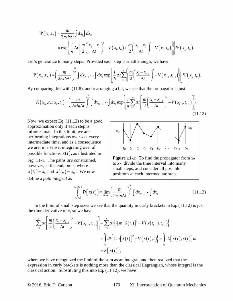
Now, we expect Eq. (11.12) to be a good
approximation only if each step is
infinitesimal. In this limit, we are
performing integrations over x at every
intermediate time, and as a consequence
we are, in a sense, integrating over all
possible functions x t , as illustrated in
Fig. 11-1. The paths are constrained,
however, at the endpoints, where
0 0x t x and N Nx t x . We now
define a path integral as
0 0
2
1 1lim .2
N NN
x t
NN
x t
mx t dx dx
i t
(11.13)
In the limit of small step sizes we see that the quantity in curly brackets in Eq. (11.12) is just
the time derivative of x, so we have
0 0
22
1 11 1 1 12
1 1
212
, ,2
, ,
,
N N
N Ni i
i i i i i
i i
t t
t t
x xmt V x t t m x t V x t t
t
dt m x t V x t t L x t x t dt
S x t
where we have recognized the limit of the sum as an integral, and then realized that the
expression in curly brackets is nothing more than the classical Lagrangian, whose integral is the
classical action. Substituting this into Eq. (11.12), we have
Figure 11-1: To find the propagator from x0
to xN, divide the time interval into many
small steps, and consider all possible
positions at each intermediate step.
t0 t1 t2 t3 t4 t5 tN
x0
xN
tN-1
…
…
XI. Interpretation of Quantum Mechanics 180 © 2016, Eric D. Carlson
0 0
0 0, ; , exp .N Nx t
N N
x t
iK x t x t x t S x t
(11.14)
This expression is certainly compact, but unfortunately it is rarely useful in performing actual
computations.1 It does, however, allow us to immediately write down an alternative form of the
second of our quantum mechanical postulates, which would now look something like
Postulate 2: Between measurements, the state vector changes according to
0
0exp ,t
t
it x t S x t t
where S x t is the classical action associated with the path x t .
I have not attempted to make the notation completely clear or generalizable, because I have no
intention of using the second postulate in this form. Indeed, it can be shown to be identical with
the second postulate we have used up to now, so it should not be considered a separate
interpretation of quantum mechanics.
Why would anyone consider this statement superior to the original version of the postulate?
Well, it isn’t mathematically simpler, since the path integral is such a beastly thing to define.
However, it has a variety of advantages. First of all, classical physics normally starts from the
Lagrangian and the action, and then works for a while before defining the Hamiltonian. This
formulation allows us to jump to the equivalent of the Schrödinger equation in a single step.
Furthermore, if you consider relativity, the Hamiltonian turns out not to be Lorentz invariant, and
if you use the Hamiltonian formulation of quantum mechanics you will end up with a lot of non-
Lorentz invariant formulas. In contrast, the action is Lorentz invariant, so this version of the
second postulate more naturally allows one to proceed to finding relativistic quantum mechanical
theories.
There is also a very nice connection between Eq. (11.14) and classical mechanics. Consider
the fact that in terms of any ordinary dimensions, Planck’s constant is very tiny, and hence the
argument of the exponential will be a large imaginary number. If you change the path x t even
a tiny bit the action will generally change, and therefore the exponential will suddenly change its
phase. Hence when you integrate over all paths, most paths will have contributions that are
nearly cancelled by nearby paths whose phase is rapidly varying. The only exception is paths
such that tiny changes in the path produce no change in the action; to be precise, paths such that
0.
S x t
x t
(11.15)
Indeed, a common method for estimating integrals of the form Eq. (11.14) is called the
stationary phase approximation, where you assume it is dominated by paths near to Eq. (11.15).
1 You can actually solve the harmonic oscillator using this method, though it is cumbersome. In quantum
chromodynamics, the quantum mechanical theory of the strong force, perturbative and other approaches tend to fail,
and path integrals are sometimes used for brute-force computations. Such techniques take phalanxes of high-speed
computers working in parallel, and only in the last decade or two have they been able to provide any useful data.
© 2016, Eric D. Carlson 181 XI. Interpretation of Quantum Mechanics
But we recognize Eq. (11.15) from classical mechanics as simply the classical path. Hence to
leading order, in the limit where Planck’s constant is small, the path that has the largest quantum
mechanical contribution is none other than the classical path. But in quantum mechanics, the
particle takes all paths.
D. The Heisenberg Picture
Suppose we have a quantum system initially in the state vector 0t and are performing a
measurement corresponding to an operator A for a quantum system with at a later time t. Then
the expectation value of the operator is given by
†
0 0 0 0, , .A t A t t U t t AU t t t (11.16)
Up to now we have regarded the state vector as changing, while the operator A stays “constant.”
However, looking at Eq. (11.16), isn’t it equally consistent to regard the state vector as constant,
while the operator changes? Let’s define the Heisenberg version of the operator A as
†
0 0, , ,H SA t U t t A U t t
where we have used subscripts to denote the operator in the usual Schrödinger picture and the
new Heisenberg picture. This will apply even to the Hamiltonian,
†
0 0, , ,H SH t U t t H t U t t
though if H contains no explicit time dependence, then U commutes with H and therefore
H SH H . We will also define the Heisenberg state vector as
0 .H S t (11.17)
Then Eq. (11.16) can be written in either the Heisenberg or Schrödinger picture.
.S S S H H HA t A t A t (11.18)
The difference is that in the Heisenberg picture it is not the state vector but the operators that
change with time.
Can we find a simple formula for the time evolution of A in the Heisenberg picture? First
take the Hermitian conjugate of Eq. (11.3), which is
† †
0 0, , .Si U t t U t t Ht
We then use this and Eq. (11.3)to find the derivative of A:
XI. Interpretation of Quantum Mechanics 182 © 2016, Eric D. Carlson
† †
0 0 0 0
† †
0 0 0 0
† †
0 0 0 0
† †
0 0 0 0
, , , ,
, , , ,
, , , ,,
, , , ,
H S S
S S S S
S S
H HH H
S S
dA t U t t A U t t U t t A U t t
dt t t
i iU t t H A U t t U t t A H U t t
U t t H U t t U t t A U t ti iH A t A t H
U t t A U t t U t t H U t t
, .HH H
d iA t H A t
dt
Indeed, in the Heisenberg picture, we would have to rewrite the second postulate something like
this:
Postulate 2: All observables A evolve according to
, ,d i
A t H A tdt
(11.19)
where H is another observable.
If you are working in the Heisenberg picture you should rewrite the other postulates as well,
removing references to t in the state vector and adding them to the observables. Indeed, the
Heisenberg picture was developed before the Schrödinger picture. We can see from our
derivations that it is equivalent to it, but there is no way to tell which of the two representations
is “correct.” The Heisenberg picture is generally harder to deal with; for example, the
expectation value of most operators will change with time because the operators themselves are
changing with time. Furthermore, it is easier for me to imagine a description where the thing
being observed (the state vector) changes with time, while the methods of observation
(observables) are constant, but both are consistent.
Technically Eq. (11.19) is correct only for operators that contain no explicit time
dependence; if there is explicit time dependence there will be an additional term A t on the
right-hand side. I particular note that if the Hamiltonian has no explicit time dependence,
Eq. (11.19) shows that it will have no time dependence at all.
Let’s do a simple example to illustrate how things work in the Heisenberg picture. Consider
a single free particle in one dimension, with Hamiltonian 2 2H P m . Note first that the
momentum operator commutes with this Hamiltonian, and therefore by Eq. (11.19) it will be
constant, so that 0P t P . In contrast, the position operator does not commute with the
Hamiltonian, and we have
21 1, , , , ,
2 2
d i i iX H X P X P P X P X P P
dt m m m
with solution
1
0 0 .X t X P tm
(11.20)
© 2016, Eric D. Carlson 183 XI. Interpretation of Quantum Mechanics
This equation is identical with the classical equation of motion. Note that not only is the position
operator at different times different, it doesn’t even commute with itself:
1
, 0 0 0 , 0 0 , 0 .t i t
X t X X P t X P Xm m m
We know that any operators that don’t commute lead to an uncertainty principle, and using
Eq. (4.15) this would take the form
0 .2
tx t x
m
Though this could be proven directly with the Schrödinger picture, it is easiest to prove in the
Heisenberg picture.
Yet another variation is the so-called interaction picture. Suppose the Hamiltonian consists
of two parts, H0 and H1, and to simplify we’ll assume H0 has no time dependence, so
0 1 .H H H t
Then it is possible to assume that the state vector evolves due to H1, while the operators change
due to H0; in other words
1 0, and , .d d i
i t H t t A t H A tdt dt
(11.21)
You can build up a perfectly consistent view of quantum mechanics treating Eq. (11.21) and as
postulates. Clearly, it is not intellectually satisfying to do so, so why would anyone ascribe to
such an approach? The answer is that it often has great practical value. Suppose H0 is large, and
easy to solve and understand, while H1 (the interaction) is smaller, and perhaps more confusing.
Then it is sometimes helpful to think of quantum states as unchanging due to H0, while the
interactions cause the state to evolve. This is effectively what we will do when we do time-
dependant perturbation theory, though we won’t actually work in this formalism. Furthermore,
in relativistic quantum mechanics, also called quantum field theory, it is not the position of a
particle R that plays the role of an observable, but a field at a point, something like E r . In the
Schrödinger picture, this operator depends on space, but not time. By switching to the
interaction picture, our field operators will depend on time as well, ,tE r , which makes it
easier to make the theory Lorentz invariant.
E. The Trace
Before moving on to the next subject it is helpful to define the trace of an operator. Let
be a vector space with orthonormal basis i , then the trace of any operator A is defined as
Tr .i i ii
i i
A A A
In matrix notation, the trace is just the sum of the diagonal elements. The trace may look like it
depends on the choice of basis, but it does not, as is easily demonstrated:
XI. Interpretation of Quantum Mechanics 184 © 2016, Eric D. Carlson
Tr
Tr .
i i i j j i j i i j j j
i i j i j j
A A A A A
A
A few properties of the trace are in order. If A and B are two operators, then it is easy to see
that
Tr
Tr .
i i i j j i
i i j
j i i j j j
i j j
AB AB A B
B A BA BA
It is important to realize that the trace is not invariant under arbitrary permutations of the
operators (like the determinant), but only under cyclic permutations, so for example, if A, B, and
C are all operators then in general
Tr Tr Tr Tr Tr Tr .ABC BCA CAB ACB CBA BAC
A general trace reduces an operator to a pure number, but when your vector space is a tensor
product space, it is sometimes useful to take only a partial trace. For example, if our vector
space is , with basis states ,i jv w , then we can perform a trace on only one of the two
vector spaces as follows:
Tr , , .j i j i k k
i j k
A w v w A v w w
This cumbersome expression is probably clearer if we write it in components:
,Tr .ki kjijk
A A
Such traces will prove useful, for example, when we have two particles, one of which we wish to
ignore. The trace on reduces the operator A from an operator acting on to one acting
only on .
F. The State Operator, or Density Matrix
One of the aspects of quantum mechanics that many find distasteful is the inherent role of
probability. Probability, of course, is not new to quantum mechanics. For example, when we
pull a card off the top of a deck, we might say there’s a 25 percent chance that it is a heart, but
this does not imply that we believe the cards are in a superposition of quantum states, which
collapses into a single suit the moment we observe the card. Instead, we are expressing only our
ignorance of the situation. Most physicists are not bothered by this role of probability. But even
though we have discussed extensively quantum probability, even including it in our postulates,
we have not discussed this more benign notion of probability resulting from ignorance.
Suppose we do not know the initial quantum state, but instead only know that it is in one of
several possible states, with some distribution of probabilities. We might describe such a system
© 2016, Eric D. Carlson 185 XI. Interpretation of Quantum Mechanics
by a list of states and probabilities, ,i it f , where i t represent a list of possible
quantum states (normalized, but not necessarily orthogonal), and fi represents the probabilities of
each state. The probabilities will all be positive, and their sum will be one:
0 and 1.i i
i
f f
We now define the state operator, also known as the density matrix, as
.i i i
i
t f t t (11.22)
What properties will this state operator have? Well, consider first the trace
Tr ,j i i i j i i j j i i i i i
j i i j i i
f f f f
Tr 1. (11.23)
Note also that its expectation value with any state vector is positive
2
0i i i i i
i i
f f (11.24)
In other words, the density matrix is positive semi-definite and has trace one. It is also apparent
from Eq. (11.22) that it is Hermitian.
Like any Hermitian operator, the state operator will have a set of orthonormal eigenvectors
i and eigenvalues i which satisfy
i i i
When working in this basis, constraint Eqs. (11.24) and (11.23) become
0 and 1.i i
i
In terms of this basis, of course, the state operator is
.i i i i i
i i
(11.25)
Comparing Eq. (11.25) with Eq. (11.22), we see that we can treat the state operator as if it is
made up of a set of orthonormal states i , with probabilities i . We can also see that any state
operator satisfying Eqs. (11.23) and (11.24) can be written in the form of Eq. (11.25), which is
the same form as Eq. (11.22).
One way to satisfy Eq. (11.25) is to have all of the probability in a single state, so
i in for some n. In such a circumstance, we say that we have a pure state. It isn’t hard to
show the only way this can be achieved is to have only a single state vector i t contributing
in the sum Eq. (11.23) (up to an irrelevant overall phase), so we don’t actually have any
ignorance of the initial state vector. Whenever this is not the case, we say that we have a mixed
state.
XI. Interpretation of Quantum Mechanics 186 © 2016, Eric D. Carlson
Given the state operator in matrix form it is easy to check if it is a pure state or not. Squaring
Eq. (11.25), we see that
2 2
i i i j j j i j i i j j i i i
i j i j i
This will be the same as if all the eigenvalues are 0 or 1, which can happen only for a pure
state. Hence 2 if and only if is a pure state. If you take the trace of 2 the result will be
2 2Tr 1.i i
i i
The inequality occurs because 0 1i , and the inequality becomes an equality only if all the
eigenvalues are 0 or 1, which again implies a pure state, so
2Tr 1 is a pure state.
You can also take the logarithm of a positive definite matrix. One measure of how mixed a
mixed state is is the quantum mechanical entropy, defined as
Tr ln lnB B i i
i
S k k
where kB is Boltzmann’s constant. Entropy vanishes for pure states and is positive for mixed
states.
The evolution of the state operator can be computed with the help of the Schrödinger
equation:
1 1
,
i i i i i i
i
i i i i i i
i
d d df f
dt dt dt
f H f H H Hi i
1
, .d
t H tdt i (11.26)
It is important not to confuse the (Schrödinger picture) state operator Schrödinger equation
Eq. (11.26) with the Heisenberg evolution of observables Eq. (11.19). They look very similar,
and this is not a coincidence, but there is a sign difference. Note that if we know the state
operator at one time Eq. (11.26)) allows us to compute it at any other time; we do not need to
know the individual components i and their corresponding probabilities fi to compute the
evolution of the state operator.
Now, suppose we perform a measurement corresponding to an observable A with complete,
orthonormal basis ,a n , where a corresponds to the eigenvalue under the operator A. What is
the probability of obtaining the result a? There are two kinds of probability to deal with, the
probability that we are in a given state i to begin with, and the probability that such a state
yields the designated eigenvalue. The combined probability is
© 2016, Eric D. Carlson 187 XI. Interpretation of Quantum Mechanics
2
, , , ,i i i i i i i
i i n i n
P a f P a f a n f a n a n
, , .n
P a a n a n (11.27)
The expectation value of the operator is even easier to compute:
Tr .
i i i i i i j j iii i i j
i j i i j j j
i j j
A f A f A f A
f A A A
Hence we don’t need to know the individual probabilities and state vectors, all we need is the
state operator.
The point I am making here is that if you know the state operator at one time, you can find it
at all later times. Furthermore, you can predict the probability of obtaining different outcomes at
future times. This suggests that it is possible to rewrite the postulates of quantum mechanics
entirely in terms of the state operator. We illustrate with the first postulate:
Postulate 1: The state of a quantum mechanical system at time t can be described as a
positive semi-definite Hermitian operator t with trace one acting on a complex
vector space with a positive definite inner product.
If you are going to change this postulate you will have to change the others as well. The second
postulate (the Schrödinger equation) will get replaced by equation Eq. (11.26), and the fourth
will be replaced by Eq. (11.27). The third postulate requires no modifications. The fifth
postulate, which describes what happens immediately after a measurement, needs to be rewritten
as well. Deriving the corresponding formula would require a bit of discussion of probability
theory, but I would rather simply give the relevant postulate.
Postulate 5: If the results of a measurement of the observable A at time t yields the result a,
the state operator immediately afterwards will be given by
,
1, , , , .
n n
t a n a n t a n a nP a
(11.28)
The approach of working with only state operators has several advantages: it allows one to
simultaneously deal with both quantum and classical indeterminacy in the same language; the
irrelevant overall phase of a state vector does not appear in the state operator; and adding a
constant to the Hamiltonian obviously has no effect, since it gives no contribution to Eq. (11.26).
But the use of matrices when column vectors suffice adds a level of complexity that I would
prefer to avoid, and I also feel it is advantageous to distinguish between things that are
unknowable and things that are simply unknown.
It is also possible to combine some of these ideas; for example, we can come up with a
Heisenberg-state operator approach where the particles are described by static state operators and
it is other operators that change over time. Then the state operator changes only due to collapse
of the state operator, as given by Eq. (11.28).
XI. Interpretation of Quantum Mechanics 188 © 2016, Eric D. Carlson
It should be noted that under time evolution, pure states remain pure, and mixed states
remain mixed. To demonstrate this, simply look at the time derivative of the trace of 2 :
2 2 21 1Tr Tr , , Tr 0.
dH H H H
dt i i
The same is true of other traces of functions of the state operator, including the entropy. Thus
pure states remain pure, and mixed states remain mixed, at least under ordinary evolution,
though measurement can, in principle, return a mixed state to a pure state. This might make one
wonder how a mixed state can ever be produced. The answer will be explored in a later section
of this chapter.
G. Working with the State Operator
Whether or not you believe the postulates should be written in terms of the state operator, it
comes in handy in a great many circumstances. For example, suppose I have a single spin-1/2
particle, and I am only interested in its spin. Suppose the particle is in an eigenstate of Sz, but we
don’t know which one, so it is half the time in the state and half the time in the state .
Then the state operator is
12
1 0 1 01 1 11 0 0 1 .
0 1 0 12 2 2
(11.29)
Suppose instead we put it in an eigenstate of
cos sinz xS S S (11.30)
which has eigenvectors
1 1 1 12 2 2 2
cos sin and sin cos . (11.31)
It is then not too hard to show that the state operator is still
12
1 12 21 1 1 1
2 2 2 21 12 2
cos sin1 1cos sin sin cos ,
sin cos2 2
1 01
.0 12
(11.32)
Since Eqs. (11.29) and (11.32) are identical, the two situations are physically indistinguishable.
Thus it is not important to distinguish between them, and in either case we simply say that the
particle is unpolarized. If we need to calculate the probability of an unpolarized electron
interacting in a particular way, we don’t have to consider electrons in all possible initial states,
instead we can simply pick a basis (such as eigenstates of Sz) and then average the results for
each of the two spin states.
© 2016, Eric D. Carlson 189 XI. Interpretation of Quantum Mechanics
Consider the following commonplace situation. Suppose we have a source of particles which
produces particles in a well-defined quantum state 0 , but at an unknown time t0, so
0 0 .t
We wish to find the state vector at an arbitrary time. Formally, we can do so with the help of
Eqs. (11.1) and (11.5), rewriting it in terms of energy eigenstates:
0
0 0 0, .niE t t
n n
n
t U t t t e
If we know the exact time t0 when the wave is produced, we can now write the state operator as
0
0 0 .m ni E E t t
n m n m
n m
t t t e
However, the initial time t0 is assumed to be completely unknown. We therefore average it over
a long time interval of length T, running from 12T to 1
2T , and average over this time interval.
12
0
12
0 0 0
1lim .m n
T
i E E t t
n m n mT
n mT
t dt eT
(11.33)
Focus for the moment on the limit of the integral of t0. We can perform it to find
12
0
12
12
0 12
sin1lim lim .m n
T
m ni E E t
T Tm nT
E E Te dt
T E E T
(11.34)
Since the sine function is limited to never be bigger than 1, and the denominator blows up at
infinity, this limit is zero unless m nE E vanishes. When this expression vanishes, we see that
we have been not very careful with the integration, but it is obvious from the left-hand side of
Eq. (11.34) that the limit is just 1. In other words,
12
0
12
0 ,
1lim .m n
n m
T
i E E t
E ET
T
e dtT
If we assume that the energy levels are non-degenerate, this is the same as nm . Substituting this
into Eq. (11.33), we see that
2
0 0 0 ,m ni E E t
nm n m n m n n n
n m n
t e
2
0where .n n n n n
n
t f f
In other words, no matter what the actual state vector that is produced by our source, we can
treat it as if it is in an unknown energy eigenstate, where the probability of it being in such an
energy eigenstate is just given by 2
0n nf . For example, if we are studying scattering, we
can treat the incoming wave as if it is a monochromatic plane wave, even if it is not. We simply
have to sum over all possible energy values in the end with the probability corresponding to the
XI. Interpretation of Quantum Mechanics 190 © 2016, Eric D. Carlson
overlap of our initial state vector with the energy eigenstates. Hence if we have a source of
waves, all we need to know is the spectrum of those waves, the set of energy values, not the
details of how those waves were produced.
H. Separability
One of the odder features of quantum mechanics is the fifth postulate, or collapse of the state
vector. According to this postulate, when any property of a particle is measured, the state vector
changes instantly and everywhere. As a simple example, consider a state vector describing the
spin state of two electrons, initially in a spin-0 state, as given in Eq. (8.20):
1
200 . (11.35)
This is an example of an entangled state, because it cannot be written as the tensor product of the
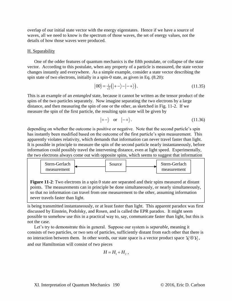
spins of the two particles separately. Now imagine separating the two electrons by a large
distance, and then measuring the spin of one or the other, as sketched in Fig. 11-2. If we
measure the spin of the first particle, the resulting spin state will be given by
or . (11.36)
depending on whether the outcome is positive or negative. Note that the second particle’s spin
has instantly been modified based on the outcome of the first particle’s spin measurement. This
apparently violates relativity, which demands that information can never travel faster than light.
It is possible in principle to measure the spin of the second particle nearly instantaneously, before
information could possibly travel the intervening distance, even at light speed. Experimentally,
the two electrons always come out with opposite spins, which seems to suggest that information
is being transmitted instantaneously, or at least faster than light. This apparent paradox was first
discussed by Einstein, Podolsky, and Rosen, and is called the EPR paradox. It might seem
possible to somehow use this in a practical way to, say, communicate faster than light, but this is
not the case.
Let’s try to demonstrate this in general. Suppose our system is separable, meaning it
consists of two particles, or two sets of particles, sufficiently distant from each other that there is
no interaction between them. In other words, our state space is a vector product space 1 2 ,
and our Hamiltonian will consist of two pieces
1 2 ,H H H
Figure 11-2: Two electrons in a spin 0 state are separated and their spins measured at distant
points. The measurements can in principle be done simultaneously, or nearly simultaneously,
so that no information can travel from one measurement to the other, assuming information
never travels faster than light.
Source Stern-Gerlach
measurement
Stern-Gerlach
measurement
© 2016, Eric D. Carlson 191 XI. Interpretation of Quantum Mechanics
where H1 and H2 affect only the vector space 1 and
2 respectively. Let the basis states for this
vector space be ,i j , where i and j are basis states for 1 and
2 respectively.
To be as general as possible, we will imagine that we describe the initial state as a density
operator with components
, , , .ij kl i j k l
Now, suppose we measure some operator A which acts only on the space 1. In other words, in
components,
, , , .ij kl i j k l i k j l ik jlA A A A
For example, we can look at the expectation value
, , , ,
Tr , , , , , ,
.
i j i j i j k l k l i j
ij ijkl
ij kl kl ij ik jl kl ij ik kj ij
ijkl ijkl ik j
A A A A
A A A
We recognize the inner sum as a partial trace, i.e., define
1 2Tr ,
then we simply have
1 1Tr .A A
where the trace is now only going over the smaller space 1 . Hence in this simple case we can
ignore the second particle (or group of particles) entirely, and work only with the first particle.
Now, suppose instead that a distant observer measures the second set of particles, using some
operator B, and determines some aspect of these other particles. The outcome of their
measurement, we will assume, is not communicated to us by conventional means, but their
measurement will inevitably cause a collapse of the state vector. Wouldn’t we notice this effect?
To make things simple, assume that the basis states j are eigenstates of B with eigenvalues
bj. Then the probability that the distant observer measures the result as bj is
,, , .j i j i j ij ij
i i
P b
Afterwards, if the result of the measurement is jb , the state operator is
,
1, , , , .J i j i j k j k j
i kjP b
However, if we do not know the result of a measurement, but only that a measurement occurs,
we must average all possible outcomes for the state operator, weighted by the corresponding
probability, so we have
XI. Interpretation of Quantum Mechanics 192 © 2016, Eric D. Carlson
,
, , , , ,j j i j i j k j k j
j j i k
P b
or in components,
, , .ij kl jl ij kj
If we now take a partial trace after the measurement on the second particle, we find
1 , , , 1 ,ij kj jj ij kj ij kj ikikj j j
i.e., the measurement on the second particle has no influence whatsoever on the collapsed state
operator1 . We can once again disregard the second particle if we are going to focus on the
first.
To illustrate these ideas more concretely, if we start in the pure state described by
Eq. (11.35), and work in a basis , , , , the initial density matrix will be
0 0 0 0 0
1 0 1 1 01 100 00 0 1 1 0 .
1 0 1 1 02 2
0 0 0 0 0
After measuring the spin of the second particle, the state vector will be in one of the two states
Eq. (11.36), with equal probability, and hence the density matrix after the measurement will be
1 12 2
0 0 0 0
0 1 0 01.
0 0 1 02
0 0 0 0
(11.37)
The collapsed density operator will be given by tracing over just the second particle. Before the
measurement, it is given by
1
0 0 0 0Tr Tr
0 1 1 0 1 01 1.
0 12 20 1 1 0Tr Tr
0 0 0 0
(11.38)
The collapsed state operator after the measurement can be found by taking a similar partial trace
of Eq. (11.37), and will be identical to Eq. (11.38). So we see that the measurement on the
distant particle 2 has no effect on the collapsed state operator.
A final concern might be that the evolution of the state operator due to Eq. (11.26) might
somehow allow faster-than light communication. The expectation value of the operator A will
evolve according to
© 2016, Eric D. Carlson 193 XI. Interpretation of Quantum Mechanics
1 2
1 1Tr Tr , Tr ,
1Tr , .
d dA A t A H t A H t
dt dt i i
A H H ti
However, since A and H2 are acting on separate spaces, they commute, and hence H2 causes no
change in the expectation values. It can further be shown that H2 causes no change in the
collapsed state operator 1 , so once again it is impossible for it to have any effect. In summary,
in a separable system, so long as we measure and interact with only one component of the
system, we can work with the collapsed state operator involving only that component, by
taking the trace over the other component. This allows one, for example, to ignore the large
(infinite?) number of particles an electron may have interacted with in the past when focusing on
that one particle. We also see clearly that using entangled states in no way provides a
mechanism for instantaneous (faster than light) communication. It is possible, of course, that
some other mechanism might provide such a means, such as a non-local term in the Hamiltonian,
but quantum mechanics per se does not demand it.
A comment is in order here: when you collapse a system from two components to one the
entropy of the system may well change. In particular, if you start with a pure state, then if you
lose track of one or more particles after an interaction, you may end up with a mixed state. As an
example, if you have two electrons in a spin-0 state (a pure state), and one of them escapes your
experiment, you will end up in a completely unpolarized state (a mixed state), if you ignore the
lost particle.
I. Hidden Variables and Bell’s Inequality
It is worth noting how different the fourth and fifth postulates concerning measurement are
from the second postulate, the Schrödinger equation. The Schrödinger equation describes the
evolution of the state vector which is continuous, predictable and reversible. It is a differential
equation, and hence continuous. It is predictable, in that there is no probability. And as argued
at the start of this chapter, the time evolution operator is unitary, which means it has an inverse,
so one can always reconstruct the initial state if you know the final state. In contrast, the fourth
postulate specifically mentions probability, and the fifth describes a discontinuous and
irreversible process. For example, suppose a spin-1/2 particle is initially in one of the two
eigenstates of Sx, that is, in one of the two states
1 1
2 2or .x x (11.39)
If we measure Sz, we will now get a plus result half of the time and a minus result the other half.
The fourth postulate states that we can only predict this in a probabilistic way. Suppose for
example that the result is now plus, then the state vector after the measurement will be .
Indeed, there is no way to deduce from the state vector afterwards which of the two states
Eq. (11.39) was the initial state.
Although we argued in section H that we cannot transmit any useful information via quantum
mechanics, it appears that quantum mechanical information is transmitted instantaneously.
Measuring the spin of one electron in an EPR pair instantly changes the other. Of course, this
XI. Interpretation of Quantum Mechanics 194 © 2016, Eric D. Carlson
instantaneous transmission of information is demanded only provided the Copenhagen
interpretation is the correct one, but there are many alternative possibilities. Let’s discuss the
concept of hidden variables. A hidden variable is some parameter in an experiment which is
unknown to the experimenter, and perhaps unknowable, which determines the outcome. As a
trivial example, suppose we take two cards, one red and one black, mix them up, place them in
two opaque envelopes, and then separate them by a large distance. Initially, we have no idea
which card is red and which is black. However, as soon as we open one envelope, we know not
only the color of that card, but the color of the other as well. There is no relativistic time delay,
and no spooky action at a distance. Could this be all that is occurring in quantum mechanics?
I would now like to demonstrate that this is not all that is going on. Consider the following
two assumptions, known as the philosophy of local hidden
variables:
1. The outcome of a particular experiment is definite; i.e., if
we could actually know all the hidden variables (and we
had the correct theory), we could predict the outcome;
and
2. It is experimentally possible to separate two particles
such that they cannot influence each other (separability).
In particular, you can separate them by performing the
measurements at widely separated points at simultaneous
(or nearly simultaneous) times, so that information
cannot be transmitted from one to the other by the
limitations of speed of light (Einstein separability).
In particular, it should be noted that these are in contradiction
with the Copenhagen interpretation, since measurement has
probabilistic outcomes, and collapse of the state vector is a non-
local event.
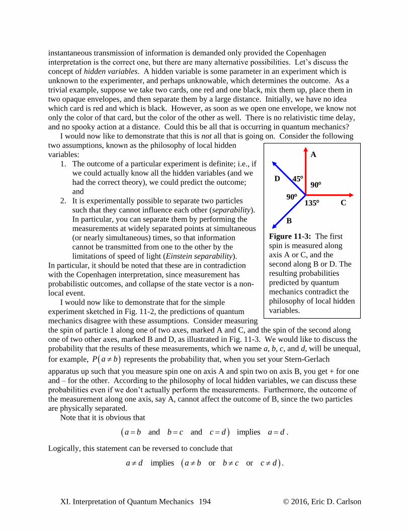
I would now like to demonstrate that for the simple
experiment sketched in Fig. 11-2, the predictions of quantum
mechanics disagree with these assumptions. Consider measuring
the spin of particle 1 along one of two axes, marked A and C, and the spin of the second along
one of two other axes, marked B and D, as illustrated in Fig. 11-3. We would like to discuss the
probability that the results of these measurements, which we name a, b, c, and d, will be unequal,
for example, P a b represents the probability that, when you set your Stern-Gerlach
apparatus up such that you measure spin one on axis A and spin two on axis B, you get + for one
and – for the other. According to the philosophy of local hidden variables, we can discuss these
probabilities even if we don’t actually perform the measurements. Furthermore, the outcome of
the measurement along one axis, say A, cannot affect the outcome of B, since the two particles
are physically separated.
Note that it is obvious that
and and implies .a b b c c d a d
Logically, this statement can be reversed to conclude that
implies or or .a d a b b c c d
Figure 11-3: The first
spin is measured along
axis A or C, and the
second along B or D. The
resulting probabilities
predicted by quantum
mechanics contradict the
philosophy of local hidden
variables.
A
C
B
D 90
135
45
90
© 2016, Eric D. Carlson 195 XI. Interpretation of Quantum Mechanics
Thus in any circumstance where a d , at least one of the other three statements must be true. In
terms of probabilities, this leads to an inequality called Bell’s inequality, named after John S.
Bell:1
.P a d P a b P b c P c d (11.40)
This prediction follows simply from the nature of the experiment and the assumptions of local
hidden variables. No assumptions about the nature of the experiment or the method of
measurement are involved. Nonetheless, this result disagrees with the predictions of quantum
mechanics.
It is easy to see from Eq. (11.35) or (11.36) that if you start with a pair of electrons in a spin-
0 state, and you measure the spin of each along the same axis, say, Sz, the resulting spins will
always come out to be opposite. Suppose instead that you measure the spin of the first along the
z-axis and the spin of the second along some other axis, S , measured at an angle compared to
the first axis, as illustrated by Eq. (11.30). The eigenvectors of S are given in Eq. (11.31). Then
it is not hard to show that the probability of getting a different result for the two spins is given by
2 12
cos .P a b (11.41)
where is the angle between the two measurements. Although the argument has been made
assuming one measurement is along the z-axis, it is actually pretty easy to show that it is valid
for any angle; all that matters is the relative angle between the two measurements.
We can use Eq. (11.41) to calculate the probability that the outcome of any pair of
measurements will be unequal. Because of the angles involved, we see that
2 12
2 12
cos 135 0.1464 ,
cos 45 0.8536 .
P a b P b c P c d
P a d
We now test this prediction against Bell’s inequality, Eq. (11.40) which would then demand
0.8536 0.1464 0.1464 0.1464 0.4391.
This inequality is clearly false, and hence quantum mechanics yields predictions that violate the
philosophy of local hidden variables.
Of course, just because local hidden variable disagrees with quantum mechanics doesn’t
mean it is incorrect. The relevant question is whether Bell’s inequality, Eq. (11.40), is violated
experimentally. Although this experiment with spins has never, to my knowledge, been done,
similar experiments involving photons have shown with a high level of confidence that Bell’s
inequality is violated.
If you wish to cling to the hidden variables philosophy, there are many possible ways of
rescuing the viewpoint. It is quite possible that the probabilistic outcome of a particular
experiment is not due to some sort of hidden variable associated with the particle, but with the
measuring apparatus. Hence, in a sense we can’t ask what the outcome of C would have been
unless the experiment is set up to measure C. One could imagine, for example, that some sort of
interaction between the measuring device and the source causes the electrons to leave the source
1 The presentation of Bell’s inequality is different than the one I usually see, but logically is a bit simpler. I suppose
I could call it Carlson’s inequality, but it is such a similar argument to the one I usually read that I don’t deserve any
credit for it.
XI. Interpretation of Quantum Mechanics 196 © 2016, Eric D. Carlson
in a different way, depending on what angle the detector for particle one is set up for. If the
experiment is set up well in advance, this transfer of information from the Stern-Gerlach device
to the source can occur slower than the speed of light.
One could imagine attempting to get around this problem by making sure to adjust the
measuring devices only at the last moment, while the electrons are en route to the devices. It is
not physically feasible to rotate the massive Stern-Gerlach devices in that short a time, but if you
instead measure the polarization of photons, it is possible to adjust the light en route based on
last-moment adjustments, for example, via a computer controlled system which chooses which
axis based on a random number generator implemented via opto-electronics. Such delayed
choice experiments have been done, in limited ways, and again confirm the predictions of
quantum mechanics. A die-hard fan might point out that computer random number generators,
despite the word “random,” are actually deterministic, and hence, in a sense, the choice is made
long before the experiment is begun. At least as a gedanken experiment, one could then imagine
replacing the computer with a graduate student with fast reactions, or perhaps slightly more
realistically, make the experiment astronomical in scale. This leads into questions of whether
graduate students (or people in general) actually have free will, which is beyond the scope of this
discussion.
For hardcore fans of local hidden variables, it should be noted that there is a loophole. All
real experiments involve a certain fraction of particles that escape the detector, and hence are
lost. For individual particles, such as electrons or photons, this loss rate is rather high.
Experimentally, you can show that the probability of getting equal or unequal results on two
spins remains pretty much constant as you increase the efficiency of your detectors. It is
normally assumed that these correlated probabilities would stay the same, even if you had perfect
detectors. Indeed, though showing experimentally that Bell’s inequality is violated requires high
efficiency detectors, it does not require perfect detectors. However, the actual efficiency to
formally demonstrate such a violation is very high, significantly higher than we can currently
achieve experimentally. It is logically and philosophically possible that Bell’s inequality is not
experimentally violated. If such is the case, then the measured disagreement rates P a b
must change in a statistically significant way as we improve our measurements. Though it is
possible to imagine such a result, it would mean a complete rewriting of much (or all) of what
we understand about physics. Every experiment would suddenly become suspect, and all of the
successes of quantum mechanics might be simply artifacts of our imperfect measuring devices.
Most physicists do not take such speculations seriously.
J. Measurement
If you look through the postulates as presented in chapter two, it is notable that three of the
five postulates concern measurement. Most physicists would have no particular trouble with the
first two postulates. True, some prefer the Heisenberg picture to the Schrödinger, which requires
rewriting the postulates a bit, or the path integral formulation, or even working with the state
operator instead of state vectors.
But the real problems come when we discuss measurement. There is nothing particularly
troubling about the third postulate, which merely states that measurements correspond to
Hermitian operators. It is the last two postulates – describing the probability of various
© 2016, Eric D. Carlson 197 XI. Interpretation of Quantum Mechanics
measurement outcomes, and how the state vector changes when you perform that measurement –
that cause concern.
What actually occurs during a measurement? As a theorist, I generally don’t want to know
how measurements are performed, but experimentally, measurements always involve
interactions between specific particles. To detect an electron, for example, one could measure
the electric force as it passes near another charged particle, or to detect a photon, one could use a
photomultiplier. If you ask an experimenter how it works, he or she will not say something like,
“well, it just collapses the state vector.” Instead there will be an explanation of how in a
photomultiplier, a photon is absorbed by a piece of metal, causing an electron to be released via
the photoelectric effect, which then moves to another piece of metal, knocking loose still more
electrons, etc., finally creating such a cascade that we can simply measure the macroscopic
current, and our computer increases its count of photons by one. The point is that there is
nothing magical about detection: it is merely a special type of interaction, or another term in the
Hamiltonian. The only thing that distinguishes measurement from some other type of interaction
is that ultimately the effects become large, large enough for us to notice it even with our unaided
senses.
If interactions represent nothing more than terms in the Hamiltonian, then we should be able
to describe its effects in terms of some sort of time evolution operator. In order to do so, we
must treat the measuring apparatus in a quantum mechanical way as well. For example, suppose
you wish to measure the spin Sz of a single electron, whose initial spin state is completely
unknown. Imagine a measuring device M with three mutually orthogonal states, 0M , M
and M , the first representing the initial state of the measuring device, before a measurement
has occurred, and the others representing the measuring device after performing a measurement
and obtaining the results + or – respectively. The initial state of the system, therefore, is
0 0 0, ,t M M
where is the electron’s spin state. If we perform a measurement on either of the states ,
we expect the interaction to lead to a time evolution operator such that the measuring device
changes its quantum state, so
1 0 0 1 0 0, , , , , , , .U t t M M U t t M M
Thus far, we have only used the Schrödinger equation to change the state vector of the system.
Consider what happens if we start in a mixed spin state, namely,
10 0 0 02
, , .x
t M M M (11.42)
Then the time evolution operator 1 0,U t t , because it is linear, must evolve this state to
11 1 0 0 2
, , , .t U t t t M M (11.43)
Thus far we have not yet collapsed the state vector. Should we? That depends on when we think
a measurement occurs. If we think of measurement as something that happens just before the
interaction with the measuring device, then we have done our analysis incorrectly. We should
split our state vector into two cases, each with 50% probability, before the interaction with the
measuring device, and analyze it something like this:
XI. Interpretation of Quantum Mechanics 198 © 2016, Eric D. Carlson
0
10 02
0
, , , 50% ,
, ,
, , , (50%).
M M
M M
M M
If, on the other hand, we think measurement occurs after the interaction, then our analysis looks
like this
1 10 02 2
, , 50% ,
, , , ,
, , 50% .
M
M M M M
M
(11.44)
Note that in each case, we see that the result is the same.
Is there any way experimentally to determine when exactly the collapse of the state vector
occurs? To do so, we would have to intervene in the intermediate state, and determine if the
state vector is a superposition, or in one of the two states. For example, suppose we measure the
expectation value of Sx, the spin along the x-axis. The initial state Eq. (11.42) can easily be
shown to have a non-zero expectation value for Sx:
10 0 0 0 0 02
1 1 10 0 0 02 2 2
, , , ,
, , , , .
x xt S t M M S M M
M M M M
Once the state vector of the electron has collapsed, however, it will be in one of the two
eigenstates , each of which has 0xS , and so this seems like a way we could tell if the
state vector has collapsed. On the other hand, using Eq. (11.43), we see that
11 1 2
1 12 2
, , , ,
, , , , 0 .
x xt S t M M S M M
M M M M
In other words, the expectation value of Sx will vanish whether or not the state vector actually
collapses. This occurs simply because the measuring device ends up in an entangled state with
the electron.
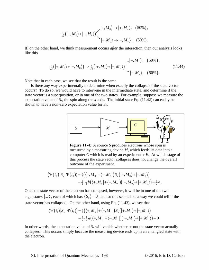
Figure 11-4: A source S produces electrons whose spin is
measured by a measuring device M, which feeds its data into a
computer C which is read by an experimenter E. At which stage of
this process the state vector collapses does not change the overall
outcome of the experiment.
S M C
E
© 2016, Eric D. Carlson 199 XI. Interpretation of Quantum Mechanics
Of course, we know that the state vector must eventually collapse, since obviously in the end
we will observe the electron to be either spin up or spin down, not both.1 To make things more
interesting, let’s imagine the measuring device M feeds its information to a computer C, which is
then read by an experimenter E, as illustrated in Fig. 11-4. We might initially describe the state
as
0 0 0 0 0 0 0, , , .s st M C E M C E
We could then imagine a process where there is a series of interactions, where first the
measuring device interacts with the electron, which then transmits the information to the
computer, whose data is read out by the experimenter. If we start in a pure spin up or spin down
state, this state will evolve according to the steps
0 0 0 0 0 0
0 0 0 0 0 0
, , , , , , , , , , , , ,
, , , , , , , , , , , , .
M C E M C E M C E M C E
M C E M C E M C E M C E
If we instead start with a spin state s x , then at each step we would end up with a
superposition, not just of the spin state, but also of the measuring device, computer, and then the
experimenter. No matter at which step the collapse of the state vector is assumed to occur, in the
end we find out that half the time the experimenter ends up learning the electron is spin up, and
half the time spin down. In summary, the predictions of quantum mechanics do not change
as you change the moment of collapse.
It is worth adding one caveat to this: you mustn’t collapse the state vector too early. For
example, it is possible to interact a single photon with a second photon such that information
about the first photon becomes entangled with the second; in essence, the second photon now
contains a “measurement” of the first photon. However, it is possible to interact the measuring
photon with the initial photon again, in such a way that it becomes disentangled. Basically, this
is just saying that if the “measurement” is sufficiently small, it is possible to reverse the process
(since the time-evolution operator is always reversible) and return to the original, pre-measured
state. Since this can be demonstrated experimentally, it follows that such small-scale
measurements must not collapse the state vector.
Ballantine argues that the state vector must ultimately collapse, since at some stage the
effects are macroscopic. This argument is incorrect. Let’s imagine, for example, that the
computer is in a superposition of two states, and the collapse happens the moment the
experimenter looks at the computer screen. Then even though the computer is in a superposition,
the experimenter will not notice.
Let’s take this to the penultimate extreme. Suppose we treat the experimenter as nothing
more than a sophisticated computer, and claim that even the experimenter doesn’t collapse the
state vector. Initially, the electron and everything is in the state
10 0 0 0 0 0 02
, , , , , ,t M C E M C E
After all the interactions, the state is
1 Things that are obvious are not necessarily true. As we will argue in the next section, it is possible to imagine a
state vector that never collapses.
XI. Interpretation of Quantum Mechanics 200 © 2016, Eric D. Carlson
13 2
, , , , , ,t M C E M C E (11.45)
We now see that the experimenter is in a superposition. Now when another physicist, say a
theorist T, asks the experimenter what the result of the experiment is, the whole thing will
collapse, placing the experimenter (finally) in a state which is no longer a superposition.
There seems to be an obvious flaw in this argument. An experimenter is not like a mindless
computer; surely she would notice she was in a superposition. We can simply ask her and find
out whether she was in the state Eq. (11.45). To consider this possibility, we expand our
description of the experiment somewhat, namely, because she is not only aware of the spin of the
electron, E , we imagine she might also be aware of whether it is in a definite, non-
superposition state dD , or an indefinite, superposition state sD .
For example, suppose a spin + electron is fed into the system, then the initial state would be
0 0 0 0 0, .t M C E D
We now let the measuring device interact, the computer receive the data, and the experimenter
see the result:
1 0 0 0, ,t M C E D
2 0 0, ,t M C E D
3 0, .t M C E D (11.46)
The experimenter now notices that her awareness of the spin state is not a superposition, and
therefore concludes it is in a definite state, not a superposition.
4 , .dt M C E D (11.47)
In a similar way, suppose we start with a spin down electron, then after reading the result off a
computer screen, the quantum state would be
3 0, .t M C E D (11.48)
Again, her awareness is not in a superposition, and hence she would conclude she is in a definite
state:
4 , .dt M C E D (11.49)
Now, suppose instead we had started in a mixed state. Then the quantum state after the
experimenter observes the computer will be
13 0 02
, ,t M C E D M C E D (11.50)
And now, at long last, we are prepared to reach a truly startling conclusion. We know that upon
introspection, the experimenter’s internal awareness will evolve from Eq. (11.46) to Eq. (11.47).
We also know that it will evolve Eq. (11.48) to Eq. (11.49) follows that Eq. (11.50), upon
introspection, will change into
© 2016, Eric D. Carlson 201 XI. Interpretation of Quantum Mechanics
13 2
, ,d dt M C E D M C E D
Note that both portions of the state vector are in the state dD ; that is, the experimenter will
incorrectly conclude that the state vector is not in a superposition, even though it is.
Hence the theorist T, when he asks whether the experimenter has measured a definite state or
a superposition, will always conclude that it is a definite state, even though no collapse has
occurred. In this picture (and the many worlds Interpretation), the universe will often consists of
superpositions of state vectors that are very different, not simply a single electron spin being up
or down, but where major events, even astronomical events, are not definite until they are
observed.
This allows one to develop a philosophy of quantum mechanics I call solipsism, where you
take the attitude that you alone are capable of collapsing the state vector. Particles, measuring
devices, computers, and experimenters may be in a superposition up to the moment you
interrogate them. One can end up in ridiculous situations, such as the famous Schrödinger’s cat,
where a cat is in a superposition of being alive and dead, until the moment you observe it. This
viewpoint is self-consistent, and has no experimental contradictions that I am aware of, but
seems remarkably egotistical. In the next section, we take this philosophy one step farther and
discuss the many worlds interpretation.
K. The Many Worlds Interpretation of Quantum Mechanics
The many worlds interpretation, or MWI, is based on the assumption that state vectors never
collapse. No one, including myself, is capable of collapsing the state vector. As such, the
postulates of quantum mechanics are reduced to just two, reproduced here for completeness:
Postulate 1: The state of a quantum mechanical system at time t can be described as a
normalized ket t in a complex vector space with a positive definite inner product.
Postulate 2: The state vector evolves according to
,i t H t tt
where H t is an observable.
And that’s it! Indeed, postulate 2 is simpler than before, since we no longer need to restrict the
Schrödinger equation to situations where measurement does not occur. Measurement is
interaction, governed by the Hamiltonian, and hence does not require a separate postulate.
It is worth mentioning that the two postulates listed above can be changed to the Heisenberg
picture, or by using path integrals, or using the state operator instead. I personally prefer the
Schrödinger picture, but don’t really have any strong feelings one way or the other.
The third postulate, namely, that measurements correspond to operators, is no longer needed,
because all measurement is governed by Hamiltonians, and since the Hamiltonian is itself an
observable, it isn’t necessary to make such a separate assumption. The fifth postulate,
concerning collapse of the state vector, is no longer necessary. This does lead to a weird picture
of the universe – one in which many possibilities coexist, in some of which this document
doesn’t exist, because the author was killed in a car accident, or was never born, or perhaps life
XI. Interpretation of Quantum Mechanics 202 © 2016, Eric D. Carlson
itself never came into existence on Earth. The possibility of “many worlds” coexisting seems
absurd, but is taken seriously by many physicists.1
This leaves only the fourth postulate. According to the Copenhagen interpretation, if we
measure Sz for an electron in the spin state x , we will get the result + or the result -, with a
50% probability of each. According to MWI, we will get both results, with a state vector that is
equal parts of each, though we will (incorrectly) believe we only got one or the other. These
results seem similar – but wait, there is a specific statement of probability in Copenhagen. This
seems a superiority of Copenhagen over MWI – it predicts a particular probability. If MWI
cannot reproduce this success, we must conclude that MWI is wrong, or at least inferior to
Copenhagen.
Well, experimentally, if we actually have only one electron, giving a probabilistic answer to
an experimental question is not really very helpful. If we measure the one electron, and the spin
comes out +, have we verified our hypothesis or not? Probabilities are not statements about
individual experiments, but rather about a series of repeated experiments in the limit that the
experiment is repeated indefinitely. Let’s imagine we have a series of N electrons, each one
initially in the state x . Suppose we measure Sz for each of these, and then average the results.
According to the Copenhagen interpretation of quantum mechanics, if you measure Sz of one of
these, you will get the result 12
half the time and 12
the other half, and over a long series of
experiments they will average to zero. Does MWI make the same prediction?
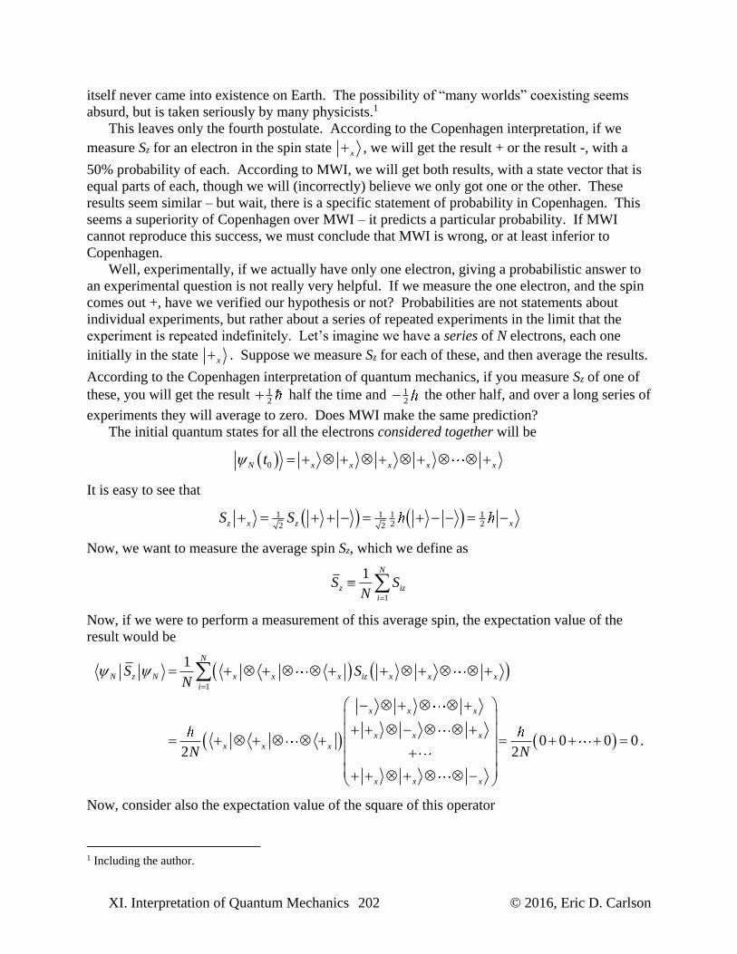
The initial quantum states for all the electrons considered together will be
0N x x x x xt
It is easy to see that
1 1 1 12 22 2z x z xS S
Now, we want to measure the average spin Sz, which we define as
1
1 N
z iz
i
S SN
Now, if we were to perform a measurement of this average spin, the expectation value of the
result would be
1
1
0 0 0 0 .2 2
N
N z N x x x iz x x x
i
x x x
x x x
x x x
x x x
S SN
N N
Now, consider also the expectation value of the square of this operator
1 Including the author.
© 2016, Eric D. Carlson 203 XI. Interpretation of Quantum Mechanics
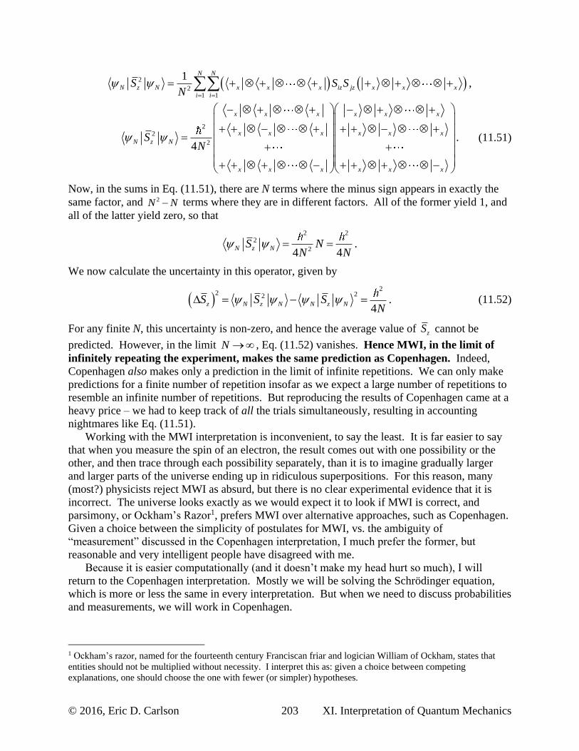
2
21 1
1,
N N
N z N x x x iz jz x x x
i i
S S SN
2
2
2.
4
x x x x x x
x x x x x x
N z N
x x x x x x
SN
(11.51)
Now, in the sums in Eq. (11.51), there are N terms where the minus sign appears in exactly the
same factor, and 2N N terms where they are in different factors. All of the former yield 1, and
all of the latter yield zero, so that
2 2
2
2.
4 4N z NS N
N N
We now calculate the uncertainty in this operator, given by
2
2 22 .4
z N z N N z NS S SN
(11.52)
For any finite N, this uncertainty is non-zero, and hence the average value of zS cannot be
predicted. However, in the limit N , Eq. (11.52) vanishes. Hence MWI, in the limit of
infinitely repeating the experiment, makes the same prediction as Copenhagen. Indeed,
Copenhagen also makes only a prediction in the limit of infinite repetitions. We can only make
predictions for a finite number of repetition insofar as we expect a large number of repetitions to
resemble an infinite number of repetitions. But reproducing the results of Copenhagen came at a
heavy price – we had to keep track of all the trials simultaneously, resulting in accounting
nightmares like Eq. (11.51).
Working with the MWI interpretation is inconvenient, to say the least. It is far easier to say
that when you measure the spin of an electron, the result comes out with one possibility or the
other, and then trace through each possibility separately, than it is to imagine gradually larger
and larger parts of the universe ending up in ridiculous superpositions. For this reason, many
(most?) physicists reject MWI as absurd, but there is no clear experimental evidence that it is
incorrect. The universe looks exactly as we would expect it to look if MWI is correct, and
parsimony, or Ockham’s Razor1, prefers MWI over alternative approaches, such as Copenhagen.
Given a choice between the simplicity of postulates for MWI, vs. the ambiguity of
“measurement” discussed in the Copenhagen interpretation, I much prefer the former, but
reasonable and very intelligent people have disagreed with me.
Because it is easier computationally (and it doesn’t make my head hurt so much), I will
return to the Copenhagen interpretation. Mostly we will be solving the Schrödinger equation,
which is more or less the same in every interpretation. But when we need to discuss probabilities
and measurements, we will work in Copenhagen.
1 Ockham’s razor, named for the fourteenth century Franciscan friar and logician William of Ockham, states that
entities should not be multiplied without necessity. I interpret this as: given a choice between competing
explanations, one should choose the one with fewer (or simpler) hypotheses.
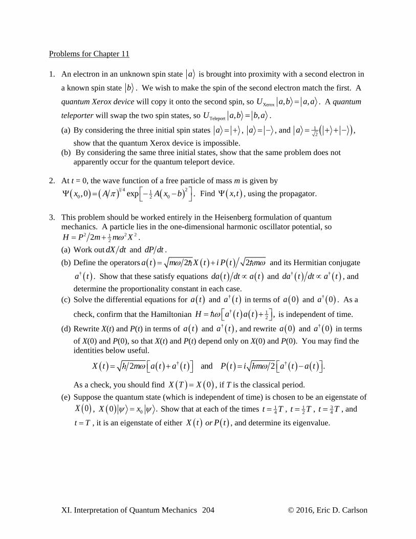
XI. Interpretation of Quantum Mechanics 204 © 2016, Eric D. Carlson
Problems for Chapter 11
1. An electron in an unknown spin state a is brought into proximity with a second electron in
a known spin state b . We wish to make the spin of the second electron match the first. A
quantum Xerox device will copy it onto the second spin, so Xerox , ,U a b a a . A quantum
teleporter will swap the two spin states, so Teleport , ,U a b b a .
(a) By considering the three initial spin states a , a , and 1
2a ,
show that the quantum Xerox device is impossible.
(b) By considering the same three initial states, show that the same problem does not
apparently occur for the quantum teleport device.
2. At t = 0, the wave function of a free particle of mass m is given by
1 4 21
0 02,0 exp .x A A x b
Find ,x t , using the propagator.
3. This problem should be worked entirely in the Heisenberg formulation of quantum
mechanics. A particle lies in the one-dimensional harmonic oscillator potential, so 2 2 21
22H P m m X .
(a) Work out dX dt and dP dt .
(b) Define the operators 2 2a t m X t i P t m and its Hermitian conjugate
†a t . Show that these satisfy equations da t dt a t and † †da t dt a t , and
determine the proportionality constant in each case.
(c) Solve the differential equations for a t and †a t in terms of 0a and † 0a . As a
check, confirm that the Hamiltonian † 12
,H a t a t is independent of time.
(d) Rewrite X(t) and P(t) in terms of a t and †a t , and rewrite 0a and † 0a in terms
of X(0) and P(0), so that X(t) and P(t) depend only on X(0) and P(0). You may find the
identities below useful.
† †2 and 2 .X t m a t a t P t i m a t a t
As a check, you should find 0X T X , if T is the classical period.
(e) Suppose the quantum state (which is independent of time) is chosen to be an eigenstate of
0X , 00 .X x Show that at each of the times 14t T , 1
2t T , 34t T , and
t T , it is an eigenstate of either X t or P t , and determine its eigenvalue.
© 2016, Eric D. Carlson 205 XI. Interpretation of Quantum Mechanics
4. An electron is in the + state when measured in the direction cos sinz xS S S , so that
12
S . However, the angle is uncertain. In each part, it is probably a good
idea to check at each step that the trace comes out correctly.
(a) Suppose the angle is 13
, with equal probability for each angle. What is the state
operator in the conventional z basis?
(b) Suppose the angle is randomly distributed in the range 1 12 2 , with all angles
equally likely. What is the state operator in the conventional z basis?
(c) Suppose the angle is randomly distributed in the range , with all angles
equally likely. What is the state operator in the conventional z basis?
(d) In each of the cases listed above, what is the expectation value of Sz?
5. A general Hermitian operator in a two-dimensional system, such as the state vector for the
spin of a spin-1/2 particle, takes the form 12
a 1 r σ , where are the Pauli matrices
given by Eqs. (7.17), 1 is the unit matrix, and r is an arbitrary three-dimensional vector.
(a) Find the eigenvalues of this matrix in general.
(b) What restrictions can be placed on a and r since is a state operator?
(c) Under what constraints will this density matrix be a pure state?
(d) Show that all four components of a and r are determined if we know every component of
the expectation value of the spin S .
(e) A particle with this density matrix is under the influence of a Hamiltonian 12 zH .
Find formulas for d dtr and da dt (four equations total).
6. There is another version of the disproof of the “local hidden variables” hypothesis that does
not require a discussion of probabilities. Consider a system consisting of three spins in the
state 1
2 .Each of these spins will be measured on either the x-axis or
the y-axis, that is, we will be measuring one of each of the following pairs:
1 1 2 2 3 3, , , , ,x y x y x y . The measurements will yield three eigenvalues, which
will be one each from the pairs 1 1,x y , 2 2,x y , 3 3,x y . Each of these eigenvalues can take
only the values 1.
(a) Consider each of the operators
1 1 2 3 2 1 2 3 3 1 2 3, , .x y y y x y y y xB B B
Show that is an eigenstate of each of these operators, and calculate the eigenvalue.
(b) According to quantum mechanics, suppose you happened to measure one of the three
combinations B1, B2, or B3. What is the prediction for the product of the results of those
measurements, x1y2y3, y1x2y3, or y1y2x3?
(c) According to the philosophy of hidden variables, the values for the products you found in
part (b) must be true, even if you don’t make those exact measurements. Based on the
three formulas you found in part (b), make a prediction for the product x1x2x3 (hint:
XI. Interpretation of Quantum Mechanics 206 © 2016, Eric D. Carlson
consider the product of the three possibilities in part (b)). This has nothing to do with
quantum mechanics!
(d) According to the philosophy of hidden variables, the product x1x2x3 must be what you
would get if you performed all three measurements in the x-direction, and then multiplied
them. Hence, the operator
1 2 3x x xA
will yield what value if you were to measure it, according to the philosophy of hidden
variables?
(e) Show that is, in fact, an eigenstate of A, but it has the wrong eigenvalue according to
the prediction of part (d).
7. In lecture I showed how MWI can account for the results when you measure a series of
electrons with spin states x . In this problem, we will instead measure the spin of
electrons with spin state 1 12 2
cos + sin .
(a) According to the Copenhagen interpretation, if we measure the spin Sz of this particle,
what results might we get, and what are the probabilities of each of these results? What
is the average value we would get for this result?
(b) Now we start working on the Multiple Worlds calculation. Define the state of N particles
as N ,.Define the average spin operator
1
1 N
z Zi
i
S SN
Write out explicitly z NS . You may find it useful to use the state
1 12 2
cos + sin in your answer.
(c) Work out the expectation values zS and 2
zS . I recommend you first write
out expressions for the quantities , , and .
(d) Show that 2 2 2sin 4zS N and show that therefore, in the limit N , the state
vector becomes an eigenstate of zS with the eigenvalue found in part (a).
© 2016, Eric D. Carlson 207 XII. Approximate Methods
XII. Approximate Methods
Up to now, we have treated nearly every problem we have encountered by using exact
methods. In the real world, we almost never are capable of finding such exact results.
Fortunately, in physics, unlike mathematics, it is common acceptable to find an approximate
answer. Physicists are interesting in comparing their theories with experimentally measurable
quantities, and for this reason, approximation methods are often as good, and sometimes better,
than exact results. Different techniques are useful in different circumstances, and we will focus
on a variety of techniques to give a flavor of the techniques that will prove most useful.
A. The Variational Method
The variational method is ideal for approximating the ground-state state vector and energy.
It is widely used for many complex systems, since it can be used for almost any problem. It is
based on the idea that the state vector with the minimum energy is the ground state. Suppose we
are given the Hamiltonian H. Let us imagine that we have already found all of the eigenstates of
this Hamiltonian, which we label , 1,2,n n , with n = 1 corresponding to the ground state.
These states satisfy
,n n nH E
With increasing energies
1 2 3 .E E E
Now, consider any state vector . Any such state vector can be written in terms of the
eigenstates, so we write
.n n
n
c (12.1)
This state vector may or may not be normalized, since
2* * .m m n n m n m n n
m n m n n
c c c c c
Now, consider the expectation value of the Hamiltonian for the state given by Eq. (12.1):
* * *
2 2 2 2
1 1 1 1 .
m m n n m n m n m n n m n
m n m n m n
n n n n n n n
n n n n
H c H c c c H c c E
c E c E c E E E c E E
(12.2)
In the final expression in Eq. (12.2), we note that 1 0nE E , so we have
1 .H
E
(12.3)
XII. Approximate Methods 208 © 2016, Eric D. Carlson
This provides us with a strict upper bound on the ground-state energy. It is clear from Eq. (12.2)
that this inequality will become an equality if all of the cn’s vanish save for c1, i.e., if we manage
to pick a state vector proportional to the ground state energy. It is also clear that if we have a bit
of the other state vectors mixed in, the error in the energy will be quadratic in the quantity cn of
the other state vectors mixed in, and therefore our approximation of the ground state energy will
tend to be pretty good if cn is small for 1n .
We can improve this considerably by considering not just a single state vector , but rather
a large number of them, and then pick the one that has the lowest expectation value Eq. (12.3).
This is done not by picking a number of dissimilar functions, but rather by picking functions that
are described by one or more parameters. We define a series of states a , where a
represents one or more variational parameters, and for each of them calculate the expectation
value of the ground-state energy,
.
HE
a aa
a a (12.4)
The result will be a (usually complicated) function of the parameter(s) a. The ground state
energy is guaranteed to be smaller than all of these. We wish to find the minimum value of this
function, which can be found by demanding that the function be stationary with respect to small
changes in the parameters a:
min
0 .i
Ea
aa
We then substitute this minimum point amin back into our function to estimate the ground state
energy
1 min .E E a (12.5)
This approximation is guaranteed to be higher than the actual ground state energy. If you pick
your state vector well, you will generally find that the resulting approximation is very good.
Furthermore, you can obtain an approximate ground-state state vector as well, which is simply
1 1 min
min min
1,
a
a a (12.6)
where the denominator is required to get the state vectlor properly normalized. However, this
state vector tends to be less-well approximated by Eq. (12.6) than the energy is by Eq. (12.5),
because the errors in the state vector tend to be linear, while the errors in the energy are
quadratic.
Let us illustrate how we can use the variational method to estimate the ground state energy of
helium. Helium has charge Z = 2, with Hamiltonian given by
2 2 2
2 2
1 2
1 2 1 2
2 21 1.
2 2e ek e k e ke
Hm m
P PR R R R
(12.7)
© 2016, Eric D. Carlson 209 XII. Approximate Methods
The two electrons must be placed in an anti-symmetric state. To a crude approximation, we
would expect the two electrons to both be in the 1s state, but with an anti-symmetric spin state,
so we might write the quantum state as
1
2,00 ,r r
where r represents the space part of the state. The spin part is completely anti-symmetric, so
the spatial part will be symmetric. If we ignore the interactions between the two electrons, the
wave function should then take the form
1 21 2
0 0
, exp exp ,Zr Zr
a a
r r (12.8)
where a0 is the Bohr radius given by 2 2
0 ea mk e and Z = 2 for helium. We have deliberately
not normalized the wave function, since the variational method doesn’t require us to do so. The
wave function (12.8) won’t be exactly right, because the electrons will repel each other. Each
electron will spend a lot of time near the nucleus, effectively canceling out part of the charge,
and hence effectively lowering the nuclear charge. This suggests that instead of Z = 2, the best
approximation might be to use Z = 1, or perhaps even better, some value in between. Instead of
guessing this value, let us make Z a variational parameter, and simply find which value of Z
minimizes the resulting energy.
To find the energy, we must find and H , where H is given by Eq. (12.7). We
will work out each piece separately, and then assemble it to find E Z . We find
1 0 2 0 0
22 3 2 62 2 23 3 2 0 0
1 2 6
0
4 2 ,2
Zr a Zr a Zr a a ad d e e d r dre
Z Z
r r (12.9a)
1 0 2 0
1 0 2 0
222 2 3 3
1 2 1 1 2 1
22 4 22 2
3 3 01 2 1 2 4
0 0
ˆ ,
Zr a Zr a
Zr a Zr a
d d i e e
ai Z Zd d e e
a a Z
P P P r r
r r r
2 4 2
2 2 01 2 4
,a
Z
P P (12.9b)
1 0 2 0 0
23 2 32 2 23 1 3 0 0 0
1 1 2 3 3
1
41,
2
Zr a Zr a Zr aa a ad r e d e d rdre
Z Z Z
r rR
2 5
0
5
1 2
1 1.
a
Z
R R (12.9c)
The remaining term is the most difficult to calculate. We start by writing down the integral in a
straightforward way.
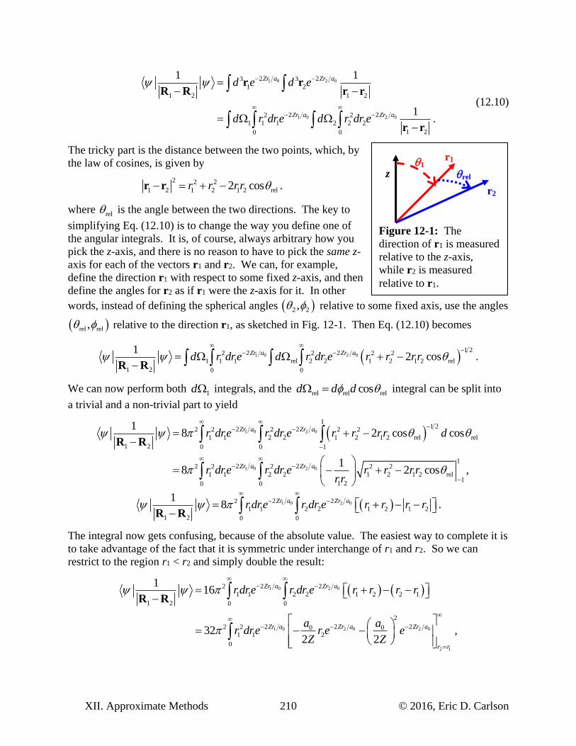
XII. Approximate Methods 210 © 2016, Eric D. Carlson
1 0 2 0
1 0 2 0
2 23 3
1 2
1 2 1 2
2 22 2
1 1 1 2 2 2
1 20 0
1 1
1.
Zr a Zr a
Zr a Zr a
d e d e
d r dre d r dr e
r rR R r r
r r
(12.10)
The tricky part is the distance between the two points, which, by
the law of cosines, is given by
2 2 2
1 2 1 2 1 2 rel2 cos .r r rr r r
where rel is the angle between the two directions. The key to
simplifying Eq. (12.10) is to change the way you define one of
the angular integrals. It is, of course, always arbitrary how you
pick the z-axis, and there is no reason to have to pick the same z-
axis for each of the vectors r1 and r2. We can, for example,
define the direction r1 with respect to some fixed z-axis, and then
define the angles for r2 as if r1 were the z-axis for it. In other
words, instead of defining the spherical angles 2 2, relative to some fixed axis, use the angles
rel rel, relative to the direction r1, as sketched in Fig. 12-1. Then Eq. (12.10) becomes
1 0 2 01 22 22 2 2 2
1 1 1 rel 2 2 1 2 1 2 rel
1 2 0 0
12 cos .Zr a Zr ad r dre d r dr e r r rr
R R
We can now perform both 1d integrals, and the
rel rel relcosd d d integral can be split into
a trivial and a non-trivial part to yield
1 0 2 0
1 0 2 0
11 22 22 2 2 2 2
1 1 2 2 1 2 1 2 rel rel
1 2 0 0 1
12 22 2 2 2 2
1 1 2 2 1 2 1 2 rel1
1 20 0
18 2 cos cos
18 2 cos ,
Zr a Zr a
Zr a Zr a
r dre r dr e r r r r d
r dre r dr e r r r rr r
R R
1 0 2 02 22
1 1 2 2 1 2 1 2
1 2 0 0
18 .Zr a Zr ardre r dr e r r r r
R R
The integral now gets confusing, because of the absolute value. The easiest way to complete it is
to take advantage of the fact that it is symmetric under interchange of r1 and r2. So we can
restrict to the region r1 < r2 and simply double the result:
1 0 2 0
1 0 2 0 2 0
2 1
2 22
1 1 2 2 1 2 2 1
1 2 0 0
2
2 2 22 2 0 01 1 2
0
116
32 ,2 2
Zr a Zr a
Zr a Zr a Zr a
r r
rdre r dr e r r r r
a ar dre r e e
Z Z
R R
Figure 12-1: The
direction of r1 is measured
relative to the z-axis,
while r2 is measured
relative to r1.
z
r1 1
rel
r2
© 2016, Eric D. Carlson 211 XII. Approximate Methods
1 0
4 32 242 3 2 20 0 0 0 0 0
1 1 12 2
1 2 0
2 218 8 6 2 ,
4 4
Zr aa a a a a ar r dre
Z Z Z Z Z Z
R R
2 5
0
5
1 2
51.
8
a
Z
R R (12.11)
We now find the energy E(Z) by using Eq. (12.4) with Eq. (12.7), substituting Eq. (12.11) and
the Eqs. (12.9) as needed:
2 2 21 2
1 2 1 2
2 4 2 2 5 2 5 2 26 2 22 20 0 0 27
82 6 4 5 5 2
0 0 0 0
2 2 1
2
2 4 5 27.
2 8 8
e
e ee
Z H Z k eE Z
mZ Z
a a a k e Z k eZ Zk e Z Z
a mZ Z Z ma a a
P P
R R R R
To find the minimum of this energy, we set the derivative equal to zero, and find
min
2
27min 8
0
0 2 .e
Z
k edE Z Z
dZ a
We therefore find 27min 16
1.6875Z , which means that effectively the nuclear charge has been
slightly reduced by the screening from the other electron. The estimate of the ground state
energy is then
2 22 2
1 min
0 0
27 27 27 2777.48 eV .
16 8 16 16e ek e k e
E E Za a
The correct experimental value is -79.01 eV, an error of about two percent. Not bad, for such a
crude approximation. The approximated ground state wave function is just given by Eq. (12.8),
normalized by multiplying it by 3 3
0Z a , where Z = 1.6875.
As we have demonstrated, the variational method is quite successful at finding the ground
state, but can it be used for higher energy states? The answer is yes. Suppose we have a
complicated Hamiltonian, and we have first found the approximate normalized ground state
vector 1 . We now create a parameterized set of approximate first excited states 2 b . We
then remove any vestige of our estimated ground state by defining
2 2 1 1 2 . b b b (12.12)
As is easily demonstrated, this state is guaranteed to have no overlap with 1 , so
1 2 0 b . Since we expect 1 to be close to the ground state, this should mean that
2 b has almost none of the ground state in it. We then find the function
2 2
2
2 2
.H
E
b bb
b b
XII. Approximate Methods 212 © 2016, Eric D. Carlson
If we minimize this function, we will have a good estimate of E2, the first excited state energy
2 2 min .E E b (12.13)
This procedure can be repeated indefinitely. However, it should be recognized that, in
general, Eq. (12.13) is not necessarily a lower bound on the first excited state energy. We have
been careful, in Eq. (12.12), to subtract our approximation of the ground state from our trial state
2 b , but there is no guarantee that we have removed all of the exact ground state. Since
there might be a small amount of the true ground state in 2 b , the resulting function E2(b)
might occasionally dip below the actual first excited state energy. There are exceptions, where
such a statement can be made, however. For example, suppose you were asked to find the
ground and first excited state for a particle in a one-dimensional symmetric potential
V x V x . We know that the ground state of such a potential will be symmetric, and the
first excited state anti-symmetric. If we pick for our trial wave function 2 b only odd
functions, 2 2x x b b , then we know that it can have no mixture of the even
ground state. Hence we are guaranteed to obtain a lower bound on the first excited state energy.
In general, the variational method works best for the ground state, and its accuracy degrades
as you increase to each of the excited states. This is because the errors accumulate as you move
up each level, eventually rendering your energy estimates poor and your state vectors poorer. A
nice complement to this method is the WKB method, which works well on excited states, but
rather more poorly on the ground state.
B. The WKB Method
The WKB method was developed shortly after the discover of the Schrödinger equation, and
works well in the classical limit, when you have much more energy than the separation between
quantum states. Although it can be used in a variety of situations, it is most easily understood
and applied to one-dimensional problems.
We start by looking at the Schrödinger equation,
2 2
2.
2
dE x x V x x
m dx (12.14)
Then if you define
2
2
2,
mk x E V x (12.15)
then Eq. (12.14) can be rewritten
2
2
2
dx k x x
dx . (12.16)
© 2016, Eric D. Carlson 213 XII. Approximate Methods
If the potential V(x) is slowly varying, then k(x) will be nearly constant, and hence the solution to
Eq. (12.16) will look something like ikxx e . This suggests writing x as the product of
an amplitude and a phase, where we would expect the amplitude to be slowly varying. We write
i xx A x e
, (12.17)
where A x and x are real functions. If x is a solution of Eq. (12.16), so is * x , so
we expect this to work for both signs of the phase. Substituting this into Eq. (12.16), we see that
2
2 2
22 ,i i id
k Ae Ae A iA A iA edx
where primes denote derivatives with respect to x, and the dependence of A and on x is
implicit. Cancelling the common phase and equating the real and imaginary parts we see that
2 2 ,Ak A A (12.18a)
0 2 .A A (12.18b)
If we define W x x , then we can multiply Eq. (12.18b) by A to yield
2 0,d
A x W xdx
which implies 1A x W x . Substituting this expression into Eqs. (12.17) and (12.18a)
yields
exp ,x
Nx i W x dx
W x
(12.19a)
2
2 2
2
3.
4 2
W WW k
W W
(12.19b)
Now, we anticipate that we are in the classical large energy limit, so we expect k to be large. To
leading order we would then anticipate that the largest term on the right side of Eq. (12.19b)
would be k2, so that W x k x . This is the zeroth order WKB approximation.1 This yields
the leading order WKB wave function, which is
exp ,xN
x i k x dxk x
(12.20)
with k(x) given by Eq. (12.15). This approximation works well only when k is large, which
corresponds to high energy.
We would like to use Eq. (12.20) to estimate the energy of bound states quickly and
efficiently. Consider first an infinite not-square well, with a potential that is infinite except in the
region a x b , but has some non-trivial potential in between, as illustrated in Fig. 12-2. Since
1 To obtain higher orders, you repeatedly substitute the expression for W in (12.19b) into itself. We will not go
beyond leading order.
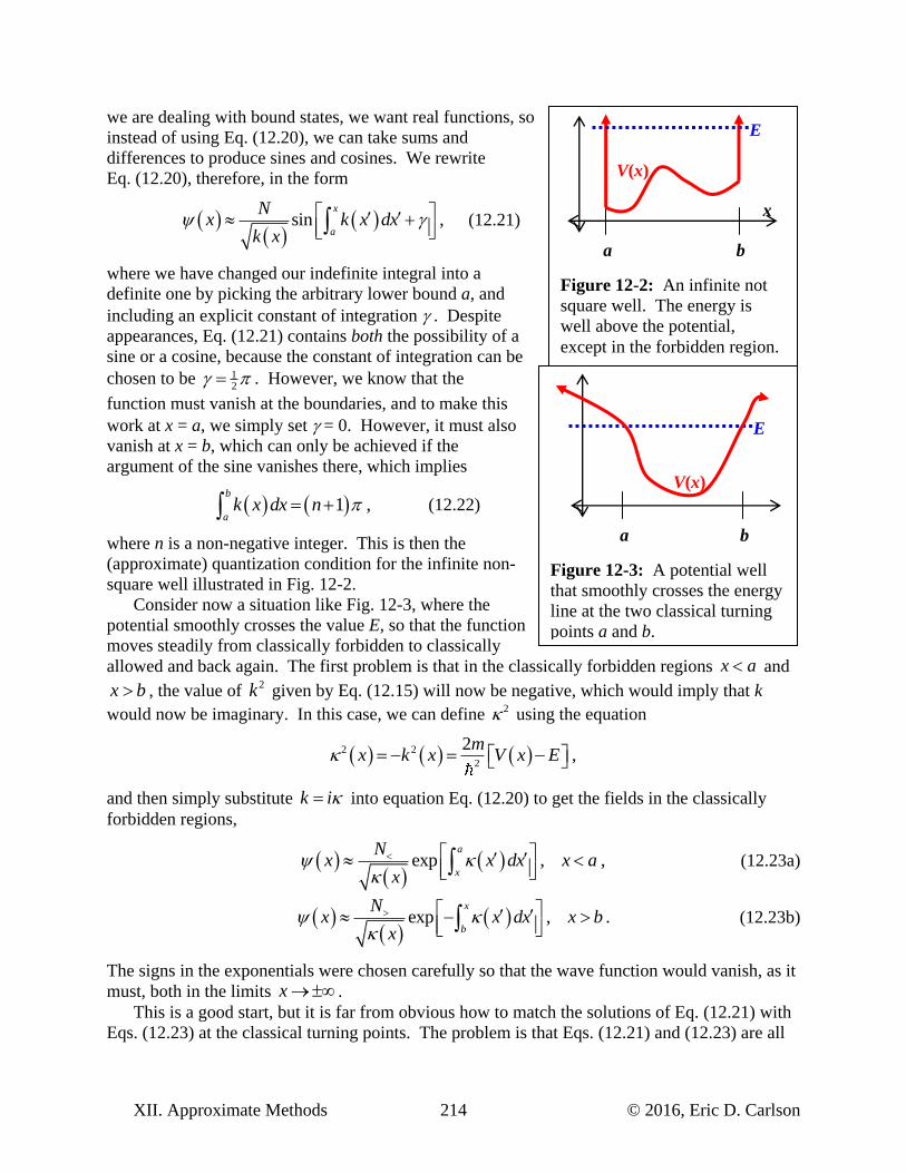
XII. Approximate Methods 214 © 2016, Eric D. Carlson
we are dealing with bound states, we want real functions, so
instead of using Eq. (12.20), we can take sums and
differences to produce sines and cosines. We rewrite
Eq. (12.20), therefore, in the form
sin ,x
a
Nx k x dx
k x
(12.21)
where we have changed our indefinite integral into a
definite one by picking the arbitrary lower bound a, and
including an explicit constant of integration . Despite
appearances, Eq. (12.21) contains both the possibility of a
sine or a cosine, because the constant of integration can be
chosen to be 12
. However, we know that the
function must vanish at the boundaries, and to make this
work at x = a, we simply set = 0. However, it must also
vanish at x = b, which can only be achieved if the
argument of the sine vanishes there, which implies
1 ,b
ak x dx n (12.22)
where n is a non-negative integer. This is then the
(approximate) quantization condition for the infinite non-
square well illustrated in Fig. 12-2.
Consider now a situation like Fig. 12-3, where the
potential smoothly crosses the value E, so that the function
moves steadily from classically forbidden to classically
allowed and back again. The first problem is that in the classically forbidden regions x a and
x b , the value of 2k given by Eq. (12.15) will now be negative, which would imply that k
would now be imaginary. In this case, we can define 2 using the equation
2 2
2
2,
mx k x V x E
and then simply substitute k i into equation Eq. (12.20) to get the fields in the classically
forbidden regions,
exp , ,a
x
Nx x dx x a
x
(12.23a)
exp , .x
b
Nx x dx x b
x
(12.23b)
The signs in the exponentials were chosen carefully so that the wave function would vanish, as it
must, both in the limits x .
This is a good start, but it is far from obvious how to match the solutions of Eq. (12.21) with
Eqs. (12.23) at the classical turning points. The problem is that Eqs. (12.21) and (12.23) are all
Figure 12-2: An infinite not
square well. The energy is
well above the potential,
except in the forbidden region.
x
V(x)
a b
E
Figure 12-3: A potential well
that smoothly crosses the energy
line at the two classical turning
points a and b.
E
V(x)
a b
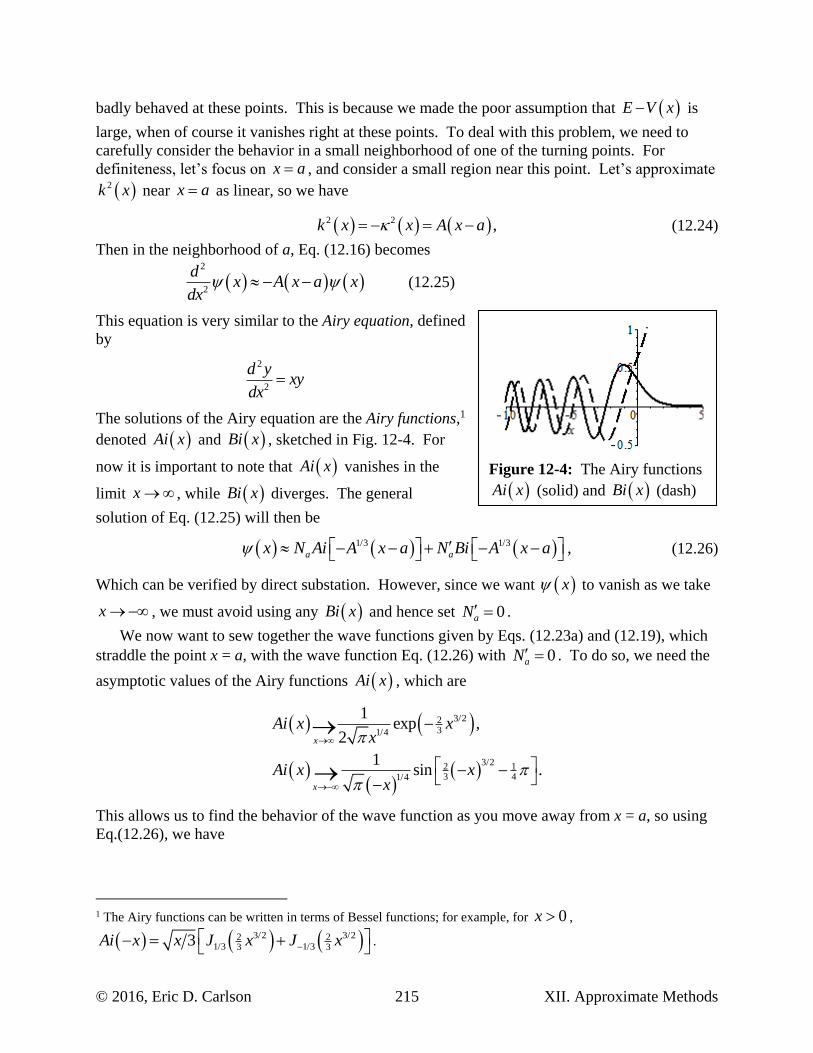
© 2016, Eric D. Carlson 215 XII. Approximate Methods
badly behaved at these points. This is because we made the poor assumption that E V x is
large, when of course it vanishes right at these points. To deal with this problem, we need to
carefully consider the behavior in a small neighborhood of one of the turning points. For
definiteness, let’s focus on x a , and consider a small region near this point. Let’s approximate
2k x near x a as linear, so we have
2 2 ,k x x A x a (12.24)
Then in the neighborhood of a, Eq. (12.16) becomes
2
2
dx A x a x
dx (12.25)
This equation is very similar to the Airy equation, defined
by
2
2
d yxy
dx
The solutions of the Airy equation are the Airy functions,1
denoted Ai x and Bi x , sketched in Fig. 12-4. For
now it is important to note that Ai x vanishes in the
limit x , while Bi x diverges. The general
solution of Eq. (12.25) will then be
1/3 1/3 ,a ax N Ai A x a N Bi A x a (12.26)
Which can be verified by direct substation. However, since we want x to vanish as we take
x , we must avoid using any Bi x and hence set 0aN .
We now want to sew together the wave functions given by Eqs. (12.23a) and (12.19), which
straddle the point x = a, with the wave function Eq. (12.26) with 0aN . To do so, we need the
asymptotic values of the Airy functions Ai x , which are
3/2231/4
3/22 13 41/4
1exp ,
2
1sin .
x
x
Ai x xx
Ai x xx
This allows us to find the behavior of the wave function as you move away from x = a, so using
Eq.(12.26), we have
1 The Airy functions can be written in terms of Bessel functions; for example, for 0x ,
3/2 3/22 21/3 1/33 3
3Ai x x J x J x
.
Figure 12-4: The Airy functions
Ai x (solid) and Bi x (dash)
XII. Approximate Methods 216 © 2016, Eric D. Carlson
3/2231/41/4
3/22 13 41/41/4
exp as ,2
sin as .
a
a
NA a x x a
A a xx
NA x a x a
A x a
(12.27)
Now, to compare these results with the results of Eqs. (12.23a) and (12.19), we use the linear
approximation Eq. (12.24), in which case Eqs. (12.23a) and (12.19) become
3/2231/41/4
3/2231/41/4
exp as ,
sin as .
NA a x x a
A a xx
NA x a x a
A x a
(12.28)
Matching Eqs. (12.27) and (12.28), we see that
14
2 and .aN N N
All this work has allowed us to determine the matching conditions across the boundary at
x a . Assuming we are not interested in the value right near the boundary, this information can
be summarized by simply saying that there is a phase shift 14
at this boundary due to the
softening of the boundary conditions, and the normalization of Eqs. (12.23a) and (12.19) are
related by 12
N N . We now must repeat the work at x b . Skipping the work, we find that
again we have 12
N N , and there is a similar phase shift of 14 at this end as well. The result
is that Eq. (12.22) gets changed to 12
n . In summary, the wave function in the classically
allowed region a x b and the quantization condition take the form
12
2 ,b
a
m E V x dx n (12.29a)
1 4
1sin 2 ,
4
x
a
Nx m E V x dx
E V x
(12.29b)
where we have used Eq. (12.15) to eliminate our function k(x), and have arbitrarily removed
some irrelevant constant factors from the (unknown) normalization. The turning points are the
places where V a V b E . As we shall see, Eq. (12.29a) allows us to efficiently estimate
the energy of all of the states.
Consider the probability density associated with the approximation Eq. (12.29b)
2
2 2 1sin 2 .
4
x
a
Nx m E V x dx
E V x
In the classical limit 0 , the oscillations become so rapid that the sine function changes too
fast to be physically measurable, and we can effectively replace sin2 with its average value, ½.
© 2016, Eric D. Carlson 217 XII. Approximate Methods
212
2 .N
xE V x
(12.30)
The denominator is proportional to the classical velocity, so the probability density is inversely
proportional to the velocity. Classically, this makes a lot of sense. Imagine a particle moving
classically in the potential sketched in Fig. 12-4, which moves from a to b and back again. If we
observe the particle at a random time, then it is unlikely we will find it at a point where it is
moving swiftly, because it will move through such positions very rapidly, and classically the
probability of finding the particle at any given point will be inversely proportional to the
velocity. Hence Eq. (12.30) agrees with the classically expected probability distribution. Hence
we can see how quantum and classical predictions correspond well, at least when the energy E is
much larger than the potential V(x).
Let’s apply our quantization rule Eq. (12.29a) to a particle of mass m contained in the
harmonic oscillator potential, 2 212
V x m x . The first step is to find the turning points,
defined as the points where V x E . Solving this equation is straightforward:
1 2
, .E
a bm
We then substitute these limits in the quantization rule Eq. (12.29a), and to the integral with the
help of Eq. (A.12g)
2
2 2 212
2
2 .
E m
E m
En dx mE m x
Solving for the energy, we have 12
E n , which is in fact exactly right. This is, however,
a coincidence that does not apply in general.
Although the WKB approach works best for one-dimensional problems, it can be applied in
more complicated cases as well. One particularly simple and interesting case is a particle in a
spherically symmetric potential. If we factor our wave function into radial and angular parts, as
we did in chapter 7, the radial part must satisfy the differential Eq. (7.27), which we repeat here
while multiplying by a factor of r.
2 2 2
2
2 2.
2 2
d l lE rR r rR r V r rR r
dr r
(12.31)
This is identical to the one-dimensional Schrödinger equation if we treat rR r as the wave
function and replace the potential V(r) with 2 2 2
eff 2V r V r l l mr . The quantization
condition Eq. (12.29a) then becomes
2
2 122
2 2 .b
a
l ldr mE mV r n
r
The turning points are generally the places where the radical vanishes, though some care must be
taken, as we shall see.
XII. Approximate Methods 218 © 2016, Eric D. Carlson
Let’s use these formulas to get an approximation for the hydrogen atom, with potential
2
eV r k e r , so we have
12 222
2 34
0 ,22
0 .
b
e
a
n lmk e l ldr mE
n lr r
(12.32)
A word is in order about the turning points, as well as the right hand side of this equation. The
upper limit b always comes by equating the expression in the radical to zero. The lower limit
also comes from setting this expression to zero provided 0l . For l = 0, there will only be one
place where the expression vanishes. However, the combination rR r appearing in Eq. (12.31)
must vanish at r = 0, and therefore we take, in this case, the lower bound to be a = 0. However,
because the combination rR r vanishes, there is no phase shift , similar to the boundary
conditions applied in Fig. 12-2, and therefore when you use Eq. (12.29a), you end up with a
factor of 34
n , rather than the usual 12
n .
With considerable work, the turning points can be found, and the integral in Eq. (12.32)
completed. The turning points are given by
2 2 4 2 22
,2
e ek e k e E l l ma b
E
.
and Eq. (12.32) works out to:
2 2
2 2 2
2
22 .
2
b
ee
a
mk e l l mdr mE k e l l
r r E
(12.33)
Equating Eqs. (12.32) and (12.33), and solving for E, we find
2 4
22 21 1
02 4
,
2
enl
l
k e mE
n l l
(12.34)
where n is any non-negative integer. The correct formula is
2 4
22.
2 1
enl
k e mE
n l
(12.35)
The difference between Eq. (12.35) and our conventional answer Eq. (7.51) occurs because we
have labeled the lowest energy state for a given l as 0n , rather than the usual notation
1n l . Comparison of Eqs. (12.34) and (12.35) reveals that the formula is not very good for
the lowest states, but considerably better as we increase l or n.
C. Perturbation Theory
Perturbation theory is one of the most powerful and useful techniques in quantum mechanics,
and indeed all of physics. Perturbation theory is most useful when you can divide your problem
© 2016, Eric D. Carlson 219 XII. Approximate Methods
into two pieces, the larger of which you can solve exactly. Assume you have a Hamiltonian of
the form
0 ,H H W
The first step is to rewrite this in the form
0H H W
where 1 The idea is to Taylor expand all quantities in powers of . The orthonormal
eigenstates n and eigenvalues n of
0H are presumed known, so that
0 and .n n n n m nmH (12.36)
Since H and 0H are close, it seems reasonable to assume that the eigenstates n and
eigenenergies En of H will be near to the eigenstates and eigenenergies of 0H . We anticipate that
we can therefore expand En and p in powers of , so that
2 ,n n n nE (12.37a)
2 .n n n n (12.37b)
We want to make sure that n is an eigenstate of H, so we need
0 .n n n nE H H W (12.38)
This alone is not sufficient to define n , since we can multiply n by any complex constant
and it will still satisfy Eq. (12.38). The easiest way to proceed is to choose this complex constant
such that 1n n to all orders in perturbation theory. Substituting in Eq. (12.37b), we see
that this implies
= = =0 .n n n n n n (12.39)
This definition does have the disadvantage that n will not be normalized, though this problem
only appears at second order in perturbation theory. It has no effect on our finding the
eigenenergies of the full Hamiltonian.
We now proceed to find the energies En to third order in and eigenstates n to second
order in . Substituting Eqs. (12.37) into Schrödinger’s Eq. (12.38) and expanding to third order
in , we have
2 3 2 3
2 3
0 ,
n n n n n n n n
n n n nH W
XII. Approximate Methods 220 © 2016, Eric D. Carlson
2
3
2 3
0 0 0ˆ ,
n n n n n n n n n n n n
n n n n n n n n
n n n n n n n nW H W H W H
where we have used Eq. (12.36) on the leading term. We now match powers of . Ignoring the
trivial leading term, this tells us
0 ,n n n n n nW H (12.40a)
0 ,n n n n n n n nW H (12.40b)
0 .n n n n n n n n n nW H (12.40c)
Of course, these formulas can be continued indefinitely as needed.
We now proceed order by order as follows. We first let the bra n act on both sides of
these equations, which allows us to get the corrections to the energies. Then we let m act on
the left side for m n . We then construct the state vectors order by order. When n acts on
the left, only the leading term will survive because of Eq. (12.39), so these equations become
0 ,n n n n n n n n n n n nW H W W (12.41a)
0 ,n n n n n n n n n n n nW H W W (12.41b)
0 .n n n n n n n n n n n nW H W W (12.41c)
The pattern is obvious. We now let m for m n act on the left of Eqs. (12.40a) and (12.40b),
but this time the first term on the left is the only one guaranteed to vanish. So we have
0
0
,
.
n m n m n m n m n m m n
n m n n m n m n m n m n m m n
W H W
W H W
We rearrange these equations to find for m n :
,m n
m n
m n
W
(12.42a)
.m n n m n
m n
n m
W
(12.42b)
We now use completeness with Eqs. (12.42a) and (12.39) to get the first order correction to the
state vector n :
.m n
n m m n m
m m n n m
W
(12.43)
We already have the first order correction to the energy Eq. (12.41a). We now substitute
Eq. (12.43) into Eq. (12.41b) to get the second order correction to the energy:
© 2016, Eric D. Carlson 221 XII. Approximate Methods
2
.m nn m m n
n m n
m n n mn m n m
WW WW
(12.44)
We also use Eqs. (12.43), (12.41a) and (12.42a) in Eq. (12.42b) for m n to obtain
2.m n n m n m i i n m n n n
m n
i nn m n m n m n i n m
W W W W W
Again, we use completeness and Eq. (12.39) to get the second order correction to the state
vector:
2.m i i n m n n n
n m m m m
m m n i n n m n i n m
W W W W
(12.45)
We can then substitute this in Eq. (12.41c) to get the third order correction to the energy:
.n m m i i n m n n n
n
m n i nn m n i n m
W W W W W
(12.46)
The procedure can be repeated to whatever order is desired. We can now substitute
Eqs. (12.41a), (12.43), (12.44), (12.45), and (12.46) into Eqs. (12.37a) and (12.37b), and use
1 . We then have
2
,
m n
n n n n
m n n m
n m m i i n m n n n
m n i nn m n i n m
WE W
W W W W W
(12.47a)
2.m n m i i n m n n n
n n m
m n i nn m n i n m n m
W W W W W
(12.47b)
We keep only the first two terms if we want to do first order perturbation theory. Note that
Eq. (12.47b) is not normalized, though it is normalized to first order.
Before proceeding, let us consider the validity of our approximation. When doing
perturbation theory, a good technique is to do the calculation to the highest order you can
conveniently calculate, then see whether each term in the series is smaller than the previous one.
Consider, for example, the energy. Let’s compare the second correction to the first. Let’s
assume that the state m nearest in energy to the state we are interested in n is separated by
an energy gap from it, so that
for .n m m n
Then the denominators in the second correction in Eq. (12.47a) will always be bigger than ,
which gives an upper bound on this term of
XII. Approximate Methods 222 © 2016, Eric D. Carlson
2 2 22
.m n m n m n n m m n n n
m n m n m n mn m n m
W W W W W W
The expression on the left is the second order correction to the energy; the expression on the
right resembles the first order correction, but with an extra factor of W in the numerator and a
factor of in the denominator. In other words, perturbation theory works well when the size of
the perturbation is small compared to the splitting between levels. Provided is non-zero, and
the perturbation W is small enough, we can always be sure perturbation theory will work.
Let’s do a simple example to see how to use Eqs. (12.47a) and (12.47b). Consider a
Hamiltonian
2 2 2 412
1,
2H P m X X
m
where is assumed small. The first two terms we name H0 and recognize as the harmonic
oscillator, with quantum states n with energies 12n n . Our perturbation is 4W X .
Let’s find the second order correction to the ground state energy and first order correction to the
state vector. Taking advantage of raising and lowering operators, we find
2 2 24 3 2
4 † † †
2 2 2 2
2 2†
2 2 2 2
0 0 0 1 2 2 02 4 4
6 3 3 1 24 4 6 2 2 3 0 .4 4
W X a a a a a am m m
a am m
The energy is then
2 2 22
10 0 2 2 2
0 0
22 2 2 2 3
1 12 22 2 2 2 2 2 4 5
0 2 0 4 030 0
4 2 4
3 72 24 3 21.
4 4 2 4 4 8
q q
q W W WE W
m
m m m m
The ground state vector, to first order, is
0 2 30 0
0 2 0 4 00 0 2 4 0 6 2 2 6 4 .
2 4 8q q
q W W Wq
m
D. Degenerate Perturbation Theory
When we look at equations Eqs. (12.47a) and (12.47b), a problem quickly comes to mind.
What do we do if two or more unperturbed states have the same unperturbed energy? If n m ,
then we have vanishing denominators, and Eqs. (12.47a) and (12.47b) will yield nonsensical
results. Hence it is clear perturbation theory, as described in the previous section, will fail. Of
course, it is always possible we will get lucky, and the numerators m nW will vanish. If we
© 2016, Eric D. Carlson 223 XII. Approximate Methods
could somehow assure that this will vanish, then in fact all the previous calculations will work
just fine, and we can proceed as usual. This is the key to degenerate perturbation theory.
Suppose we have a set of states 1 2, , , g , all of which have the same unperturbed
energy, so,
0 , 1,2, , .i iH i g
Then the same will be true of any linear combinations of the eigenstates i . Our goal,
therefore, is to find orthonormal states i which are linear combinations of the i ’s, but such
that j iW vanishes when i j . To do this, let’s define the matrix W , a finite square matrix
of size g g , with matrix elements ij i jW W , so
1 1 1 2 1
2 1 2 2 2
1 2
.
g
g
g g g g
W W W
W W WW
W W W
We first find the orthonormal eigenvectors iv of W , so that
†, and for , 1, , .i i i i j ijW w i j g v v v v
Then we can define a new set of eigenstates
1
,g
i i jjj
v
where i jv is the j’th component of
iv . Then it isn’t hard to show that
and .j i i ij j i ijW w
In other words, W is diagonal in the new basis when restricted to the degenerate states with
energy i . We then proceed with perturbation theory in the usual way, and our difficulties
have disappeared!
Note that this procedure is completed before we begin doing perturbation theory. Indeed, the
orthonormal states i are independent of how weak the perturbation W is; they are, in a sense,
zeroth order in our small parameter . This may seem surprising, but in the absence of any
perturbation, the eigenstates i are ambiguous. Only the perturbation breaks the degeneracy
and determines which are your actual eigenstates. After switching to the new states i ,
Eqs. (12.47a) and (12.47b) become
2
m n
m n
n n n n
n m
WE W
XII. Approximate Methods 224 © 2016, Eric D. Carlson
,m n i n
n m m i i n m n n n
n m n i n m
W W W W W
2.
m n i n
m m m i i n m n n n
n m m
n m n m n i n m
W W W W W
The sums have been reduced to only include terms with non-vanishing denominators. Note that
the first order correction to the energies, n nW , are simply the eigenvalues wn of the matrix
W .
As an illustration of how this is implemented, suppose we have a particle of mass m in a
perturbed two-dimensional infinite square well, with potential
1 1
3 6if 0 , ,
,otherwise,
x a y a x y aV x y
where is assumed to be small. Then the unperturbed wave functions look like
2
, sin sin ,pq
px qyx y
a a a
with energies
2 2
2 2
2.
2pq p q
ma
The ground state 11pq is non-degenerate, and we need not change basis for this state.
However, the first excited states 12pq and 21pq are degenerate, so to leading order
our eigenstates will be determined by the splitting. We first need to find the matrix W , whose
components are of the form
* 1 13 6
1 1 1 13 3 6 62
, ,
4sin sin sin sin ,
pq p qpq V p q x y x y x a y a dxdy
p p q qa
and therefore is given by
4 21 1 2 13 3 3 6
2 2 22 1 2 1 2 13 3 6 3 6
2
12 12 12 21 sin sin sin sin4
21 12 21 21 sin sin sin sin sin
9 3 3.
4 3 3 3
W WW
W W a
a
The eigenvectors of W are
1 2
11 13, and .
2 21 3
v v
© 2016, Eric D. Carlson 225 XII. Approximate Methods
with eigenvalues 23aw a and 0bw respectively. The eigenstates to zeroth order and the
energies to first order will be given by
2 2
11 12 2 2
2 2
12 22 2
5 33 12 21 , ,
2
512 3 21 , .
2
Ema a
Ema
Problems for Chapter 12
1. A particle of mass m is contained in the potential 412V x x .
(a) What symmetry does this potential have? What is the likely eigenvalue of the ground
state under this symmetry? What is the likely eigenvalue of the first excited state under
this symmetry?
(b) Consider the trial wave function 212expx Ax . Does this have the right
symmetry properties for the ground state, as given in part (a)? Calculate the normalized
expectation value of the Hamiltonian using this wave function.
(c) Minimize the expectation value and find an estimate of the ground state energy. Can we
conclude that the ground state energy is lower than this value?
(d) Construct a one-parameter trial wave function with the appropriate symmetry properties
for the first excited state. Calculate the normalized expectation value of the Hamiltonian
using this wave function.
(e) Minimize the expectation value and find an estimate of the ground state energy. Can we
conclude that the first excited state energy is lower than this value?
2. Joe Ignorant is unaware that the hydrogen atom has a known, exact solution, so he attempts
to use the variational method on it. The trial wave function he decides to try is given by
2Are r , where A is a variational parameter. Using this trial wave function, estimate the
ground state energy. Compare the result with the exact result.
3. Joe isn’t getting any smarter. He is attempting to find the ground state energy of an infinite
square well with allowed region a x a using the trial wave function (in the allowed
region) 2 2 4 41 1x x a B x a , where B is a variational parameter. Estimate the
ground state energy, and compare to the exact value.
4. A particle lies in one dimension with Hamiltonian2 2H P m F X . Using the WKB
method, our goal is to find the eigenenergies of this Hamiltonian.
(a) For energy E, find the classical turning points a and b.
(b) Perform the integral required by the WKB method.
(c) Solve the resulting equation for En
XII. Approximate Methods 226 © 2016, Eric D. Carlson
5. We never completed a discussion of how to normalize the WKB wave function Eq. (12.29b).
(a) Treating the average value of 2 12
sin , and including only the wave function in the
classically allowed region a x b , write an integral equation for N.
(b) We are now going to find a simple formula for N in terms of the classical period T, the
time it takes for the particle to get from point a to b and back again. As a first step, find
an expression for the velocity v x dx dt as a function of position. This is purely a
classical problem!
(c) Use the equation in part (b) to get an integral expression for the time it takes to go from a
to b. Double it to get an expression for T.
(d) Relate your answers in parts (a) and (c) to get a NON-integral relationship between the
normalization N and the classical period T.
6. A particle of mass m lies in one dimension with Hamiltonian near the origin of 2 2 2 31
22H P m m X X where is very small.
(a) Find the energy of all quantum states to second order in .
(b) Find the eigenstates of H to first order in .
(c) Find the expectation value n nX for the eigenstates n to first order in .
7. A particle of mass m lies in a one-dimensional infinite slightly tilted square well
if 0
otherwise
bx x aV x
where b is small.
(a) What are the normalized eigenstates and energies if b = 0?
(b) Find the eigenstates and energies to first order in b.
(c) Find the ground state energy to second order in b. If you can’t do the sums exactly, do
them numerically.
8. A particle of mass m lies in a two dimensional harmonic oscillator plus a perturbation
2 2 2 2 2 312
2 2x y yH P m P m m X Y X P , where is very small.
(a) What are the eigenstates and eigenenergies of this in the limit 0 ?
(b) Find the ground state and energy to first order and second order in respectively.
(c) Find the first excited states and energy to zeroth and first order in respectively.
9. A hydrogen atom in some combination of the n = 2 states is placed in an electric field which
adds a perturbation 2 212
W X Y where is small. Ignore any spin-orbit or hyperfine
splitting of the hydrogen atom; i.e., treat all n = 2 states of hydrogen as perfectly degenerate
before W is included.
(a) Find all non-vanishing matrix elements 2 2l m W lm for this interaction.
(b) Find the perturbed eigenstates and eigenenergies of the n = 2 states to zeroth and first
order in respectively.
© 2016, Eric D. Carlson 227 XIII. Applications of Approximate Methods
XIII. Applications of Approximate Methods
An electron in an isolated hydrogen-like atom, has approximate Hamiltonian
2
2
0
1,
2e
e
k e ZH
m P
R (13.1)
where me is the mass of the electron. The eigenstates of Eq. (13.1), ignoring spin, are described
by three quantum numbers, , ,n l m , and have energy
2 4 2
2 2.
2
e en
k e m Z
n (13.2)
This formula is not the true energy, because:
The nucleus will recoil, or move in response to the electron;
The nucleus was treated as infinitesimal, when in fact it is finite
The electron is moving fast enough that there are relativistic effects
The nucleus has spin as well, which may react with the spin of the electron
The first of these has already been treated carefully section 6E: it can be included by replacing
the electron mass m with the reduced mass 1 1 1
e Nm m , where mN is the nuclear mass. We
now consider each of the others in turn.
A. Finite Nuclear Size
The nucleus is not in fact an infinitesimal object, but instead an object of finite radius a. We
will treat the nucleus as a uniformly charged sphere of total charge Ze. The total charge inside a
sphere of radius r will therefore be
3 3
,
.
Ze r aq r
Zer a r a
Gauss’s Law can then be used to find the electric field everywhere
2
3
,E
.
e
e
k Ze r r ar
k Zer a r a
The potential energy is the negative of the integral of the force on the particle used to bring it in
from infinity:
2
22
3
,
E 3.
2 2
er
e
k Ze r r a
V r e r dr rk Ze r a
a a
(13.3)
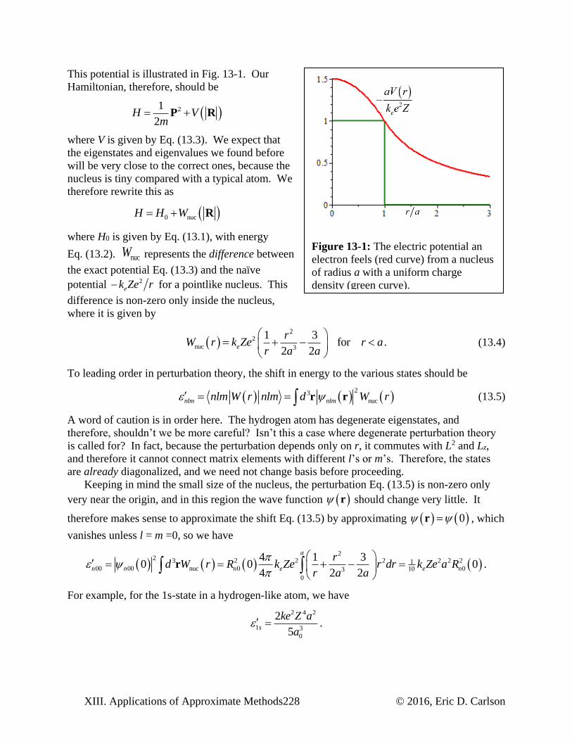
XIII. Applications of Approximate Methods228 © 2016, Eric D. Carlson
This potential is illustrated in Fig. 13-1. Our
Hamiltonian, therefore, should be
21
2H V
m P R
where V is given by Eq. (13.3). We expect that
the eigenstates and eigenvalues we found before
will be very close to the correct ones, because the
nucleus is tiny compared with a typical atom. We
therefore rewrite this as
0 nucH H W R
where H0 is given by Eq. (13.1), with energy
Eq. (13.2). nucW represents the difference between
the exact potential Eq. (13.3) and the naïve
potential 2
ek Ze r for a pointlike nucleus. This
difference is non-zero only inside the nucleus,
where it is given by
2
2
nuc 3
1 3for .
2 2e
rW r k Ze r a
r a a
(13.4)
To leading order in perturbation theory, the shift in energy to the various states should be
23
nucnlm nlmnlm W r nlm d W r r r (13.5)
A word of caution is in order here. The hydrogen atom has degenerate eigenstates, and
therefore, shouldn’t we be more careful? Isn’t this a case where degenerate perturbation theory
is called for? In fact, because the perturbation depends only on r, it commutes with L2 and Lz,
and therefore it cannot connect matrix elements with different l’s or m’s. Therefore, the states
are already diagonalized, and we need not change basis before proceeding.
Keeping in mind the small size of the nucleus, the perturbation Eq. (13.5) is non-zero only
very near the origin, and in this region the wave function r should change very little. It
therefore makes sense to approximate the shift Eq. (13.5) by approximating 0 r , which
vanishes unless l = m =0, so we have
2
2 3 2 2 2 2 2 2100 00 nuc 0 0103
0
4 1 30 0 0 .
4 2 2
a
n n n e e n
rd W r R k Ze r dr k Ze a R
r a a
r
For example, for the 1s-state in a hydrogen-like atom, we have
2 4 2
1 3
0
2.
5s
ke Z a
a
Figure 13-1: The electric potential an
electron feels (red curve) from a nucleus
of radius a with a uniform charge
density (green curve).
© 2016, Eric D. Carlson 229 XIII. Applications of Approximate Methods
For hydrogen, this is smaller than the binding energy of the 1s state by a factor of 2 2
04 5a a , or
about 10-10, which is smaller than most of the other perturbations we will consider. The shift in
energy is difficult to see in any case, since usually differences in energy are easier to measure
than a shift in a specific level. In contrast, the shift in the 2s state is easier to measure, since it is
(nearly) degenerate with the 2p state, even though the shift itself is eight times smaller. For
heavier hydrogen-like atoms, the shift increases by a factor of Z4, and is further enhanced by the
larger nuclear radius a, but it is still a small effect (also, the binding energy of the electron has
increased by Z2 as well), though noticeable. If the electron is replaced by the much heavier
muon ( 207em m ), the radius a0 decreases by the ratio of masses, enhancing this effect
enormously, and allowing one to effectively measure the radius a of the nucleus.
B. Spin-Orbit Coupling
In addition to finite nuclear effects, which tend to be quite small, there are significant
relativistic effects. An electron in the ground state of a hydrogen-like atom has a typical velocity
of about v c Z , where 1137
is the fine structure constant.
A proper treatment of relativistic effects requires the Dirac Equation, the subject of a later
chapter, and we will not go into it here. The one that interests us at the moment is the spin-orbit
coupling, the only one of these interactions that depends on spin.
Spin-orbit coupling can be seen as an effect of interactions between the magnetic dipole
moment of the spinning electron as it moves in the presence of an electric field. As can be
shown from relativity, a moving object in an electric field experiences, in its own frame, a
magnetic field, which to leading order at small velocities v is given by
2 2
1 1,U
c mc B v E p r
where U(r) is the electrostatic potential. A magnetic dipole m in a magnetic field experiences an
energy shift
2
1.E U
mc B m p r m
If we then substitute the magnetic moment 2gq mm S of the electron from section 9D, we
would anticipate an energy shift of the form
2 2 2 2.
2 2c
gq gE U V
m c m c p r S p r S
where cV qUr r is the Coulomb potential experienced by the electron. Since cV r is
spherically symmetric, the resulting classical energy shift in the electron would be
2 2 2 2
1ˆ ,
2 2
c cdV r dV rg gE
dr m c m c r dr p r S L S (13.6)
where L r p is the angular momentum. Now, (13.6) was derived working in the rest frame of
the electron. Do we get the same answer if we work in the rest frame of the nucleus? In this
XIII. Applications of Approximate Methods230 © 2016, Eric D. Carlson
frame, there is no magnetic field, and hence the energy “shift” due to the magnetic moment of
the electron is simply 0E . Which equation, Eq. (13.6) or 0E , is the correct one to use?
The answer cannot be found without a relativistic theory of the electron, but it turns out that the
right approach is to take the average of these two. We will do so, and now reinterpret E as a
perturbation WSO on the Hamiltonian.
SO 2 2
1,
4
cdV rgW
m c r dr L S (13.7)
where g = 2.00 for an electron.
What will be the effect of W on the quantum states of hydrogen-like atoms? Before
proceeding, we must expand our basis states , ,n l m which normally describe hydrogen to
include the spin state, so our states now look like , , ,l sn l m m . However, in hydrogen we have
degeneracy between various states with the same principle quantum number n. According to
degenerate perturbation theory, we must now calculate all the matrix elements of the form
, , , , , ,l s l sn l m m W n l m m . For arbitrary n, this looks like quite a task, since there are 2n2 total
states, so we would end up having to then diagonalize 2 22 2n n matrix.
Fortunately, things are not as bleak as they seem. Our perturbation W commutes with 2L ,
and therefore it cannot connect states with different l values. This makes things easier, but still a
bit unwieldy. Our interaction will connect states with different ml and ms values, which is still
more work than we want to do.
Fortunately, we can do better. The problem is that we originally chose eigenstates defined by
the four commuting operators 2
0 , , ,z zH L SL . When the only terms in the Hamiltonian were all
in H0, this made sense, since they all commute with H0. But rotation of only the wave function
or only the spin is no longer a symmetry of the total Hamiltonian. The new term Eq. (13.7)
remains unchanged only if you rotate the wave function and the spin together. This suggests
working with J L S , the total angular momentum, rather than with L and S separately.
Instead of using the eigenstates we have worked with up to now, let’s use eigenstates defined
by the operators 2 2
0 , , , zH JL J with states , , , jn l j m . Because Eq. (13.7) commutes with all
of these operations except for H0, the only degenerate states W connects are states with
themselves. We can also use a standard trick we learned long ago to deal with the spins and
angular momentum appearing in Eq. (13.7), so we have (taking advantage of the fact that 2 23
4S and 2g ):
SO 2 2
2 2 2
2 2
1, , , , , , , , , , , ,
4
1, , , , , , ,
8
c
j j j j
c
j j
dV rgn l j m W n l j m n l j m n l j m
m c r dr
dV rgn l j m n l j m
m c r dr
L S
J L S
2
2 2 3SO 42 2
1, , , , , , , , , , , , .
4
c
j j j j
dV rn l j m W n l j m j j l l n l j m n l j m
m c r dr
There is no angular dependence in the matrix element, so we can reduce this to a simple radial
integral. Note that the result is independent of mj; this is inevitable since J commutes with the
© 2016, Eric D. Carlson 231 XIII. Applications of Approximate Methods
Hamiltonian. Now, what is most interesting is the difference between energy levels, and since
the only possible values for j are 12
j l , we find
1 12 2
22 2
, , , , 2 2
0
12 1 .
4
c
nln l l n l l
dV rE E l r dr R r
m c r dr
(13.8)
Of course, this only makes sense for l > 0; for l = 0 there cannot be such a splitting, since only 12
j is allowed. It is now a straightforward matter to substitute the explicit form of the
Coulomb potential 2
c eV r k e r into Eq. (13.8) and calculate, for example, the splitting
between the 2p3/2 and 2p1/2 states of hydrogen.
It is useful to get some idea of the magnitude of Eq. (13.8). For hydrogen, the factor of 1/r
and the derivative each tend to bring in a factor of order 1
0a , and the average value of the
Coulomb potential is of order the binding energy of hydrogen. Ignoring numerical factors,
therefore, this splitting is of the order
2 42
2
SO 2 2 2 2 2
0
,ek eE E E E
m c a c
where 1137
is the fine structure constant. One might be tempted to naively calculate other
splittings, such as between 2s1/2 and 2p1/2. This turns out to be a mistake. In addition to the spin-
orbit coupling, there are other relativistic effects; for example, there is an additional term in the
Hamiltonian, 4 3 28m cP , which comes from the difference between the relativistic and non-
relativistic formulas for kinetic energy. The contribution of this term turns out to be exactly the
same magnitude as the contribution from WSO. It is, however, independent of spin, and hence
formulas like Eq. (13.8) will still be valid. However, if we are truly working with a hydrogen-
like atom, we should use the full Dirac equation, which can be exactly solved in this case, and
therefore equation Eq. (13.8) is not really necessary anyway.
The real value of an equation like Eq. (13.8) is not for hydrogen-like atoms, but rather for
alkali metals. For example, sodium has eleven electrons, which (in the ground state) have
electron configuration 1s2 2s2 2p6 3s1. Because of the screening of the inner electrons, the
outermost electron effectively sees a nucleus with charge +1, except for the relatively rare
fraction of the wave function which penetrates inside the inner “core” electrons. Hence sodium
looks a great deal like hydrogen, except for a significant variation in the Coulomb potential
(which is why we wrote the Coulomb potential in the general form cV r ). The variation in the
potential causes the 3s (actually, 3s1/2) electron to be about 2 eV lower in energy than the 3p
states. Because of the spin-orbit coupling, the 3p states are split, such that the 3p1/2 state has
slightly less energy than the 3p3/2. When an electron moves from the 3p to the 3s state, a single
photon will be emitted, but the exact wavelength of that photon will depend on the spin state the
electron started in. The spectrum of sodium has a very distinctive yellow appearance, which is
made of these two lines at 588.9950 nm and 589.5924 nm. The spectral line from the shorter of
these two wavelengths has an intensity twice as strong as the other, because there are twice as
many spin states for the 3p3/2 electrons as the 3p1/2 electrons, and these states become populated
in excited atoms in equal proportion.
XIII. Applications of Approximate Methods232 © 2016, Eric D. Carlson
C. Hyperfine Splitting
As already discussed, since the laws of physics are apparently invariant under rotation, one
would anticipate that the full Hamiltonian H commutes with the total angular momentum J, and
hence atoms which differ only by their mj value should be truly degenerate. This argument fails
for the simple reason that the J is not truly the total angular momentum. In addition to the orbital
angular momentum of the electron L about the nucleus and the electrons spin S, the nucleus
itself will often have a spin I. Like the electron, this means that the nucleus (which, for
hydrogen is normally just a proton) may have a magnetic moment pm , which will take the form
,2
p
p
p
g e
mm I (13.9)
Since the nucleus is so much smaller than the atom, we can treat this as effectively a point source
of magnetism. The vector potential and magnetic field from such a source is beyond the scope of
this book, but can found in standard textbooks:1
0
3,
4p
r
A r m r (13.10)
We would then calculate the magnetic field from B A , which with the help of Eq. (A.18e)
naively yields, for 0r ,
0
3ˆ ˆ3
4p p
r
B r r m m (13.11)
There is, howevever, a problem with Eq. (13.11). If one were to integrate it over angles, one
can show the integral vanishes (see problem 13.3), suggesting that the integral of the magnetic
field over all space vanishes. However, we can integrate B A over a spherical volume of
radius r with the help of Eq. (A.20), which will yield
00
2ˆ ˆ ˆ
4 3p pdV dV dA d
B A r A r m r m
And yet, how can we reconcile this result with the magnetic field given by Eq.(13.11)? The
answer is that Eq.(13.11) was calculated only away from the origin, and special care must be
taken at this point. To make the integral come out right, we must add a contribution to the
magnetic field which is non-vanishing only at the origin, and whose integral is 203 p m . This
suggests that the correct magnetic field everywhere, including the origin, is actually
3003
2ˆ ˆ3 .
4 3p p p
r
B r r m m m r (13.12)
where 7 2
0 4 10 N/A is the permittivity of free space.
We now need to add these contributions to the Hamiltonian. We first expand our
Hamiltonian Eq. (9.20) (approximating g = 2 for the electron) as
1 See, for example, Jackson, Classical Electrodynamics, Third Edition, Eq. (5.55). (© 1999, Wiley)
© 2016, Eric D. Carlson 233 XIII. Applications of Approximate Methods
2 22 2
2 21.
2 2 2 2e ek e k ee e e e
H em m m m m m
P
P A B S P A A P A B SR R
We recognize the first two terms as H0, the unperturbed Hamiltonian. We ignore the A2 term,
since we assume the magnetic field of the nucleus is small. We substitute Eq. (13.12) and the r >
a formula from Eq. (13.10) into this equation. The vector potential has no divergence, so
P A A P , and we find
30HF 3 3
1 1 8ˆ ˆ3 .4 3
p p p p
eW
m R R
μ R P R S R μ μ S R μ S
If we now substitute in the specific form Eq. (13.9) for the magnetic moment of the proton, we
have
2
0 3
HF 3 3
1 1 8ˆ ˆ3 .8 3
p
p
g eW
mm R R
I L R S R I I S R I S (13.13)
where we have simplified the first term using I R P R P I L I .
If we look at the form of Eq. (13.13), it is clear that the last term will contribute only for s-
waves, since the wave function vanishes at the origin for 0l . In contrast, the first term vanishes
for s-waves, because of the angular momentum operator. What is, perhaps, less obvious is that
the middle term also vanishes for s-waves. We can rewrite this middle term as
3 3,
1 1ˆ ˆ ˆ ˆ3 3 ,j k jk j k
j k
R R S IR R
R S R I I S
and when this is integrated for an s-wave, we get expressions like ˆ ˆ3 j k jkr r d , which can be
shown to vanish. Hence, when considering first-order perturbation theory, we need only include
the last term in Eq. (13.13) for s-waves, and the other terms for all other modes.
A complete basis for the bound states of hydrogen, ignoring perturbations, would look like
, , , ,l s In l m m m , where the last quantum number describes the eigenstate of the proton’s spin
under Iz. As already described, the spin-orbit coupling causes a splitting of states with the same
n and l, which suggests that a better basis would be , , , ,j In l j m m . Until we include the
hyperfine splitting, the states with different values of mj and mI must be degenerate, but the
hyperfine interaction Eq. (13.13) will cause splittings. Again, we have to deal with degenerate
perturbation theory, and again, the logical way to proceed is to change basis. The full
Hamiltonian, including Eq. (13.13), does not commute with L, S, or I, nor even the combination
J L S , since that is not truly the total angular momentum. The total angular momentum is
, F J I L S I
and F must commute with the full Hamiltonian, even if we have missed other perturbations. We
therefore change basis to , , , , fn l j f m , where the new quantum numbers are defined by their
eigenvalues
XIII. Applications of Approximate Methods234 © 2016, Eric D. Carlson
2 2 2, , , , , , , , ,
, , , , , , , , .
f f
z f f f
n l j f m f f n l j f m
F n l j f m m n l j f m
F
The new interactions cannot connect states with different values of mF, and therefore they are
much simpler in this new basis.
Let’s complete the computation for the s-wave states of hydrogen. These states have l = 0,
and when combined with the spin of the electron, they must have 12
j . The proton is also spin
12
i , so the total spin f must take on values from 0 to 1, with mf running form –f to f. Keeping
in mind that only the last term of Eq. (13.13) can contribute to the 1s state, we have
2
0 31 1 1 1HF2 2 2 2
,0, , , ,0, , , ,0, , , ,0, , , .3
p
f f f f
p
g en f m W n f m n f m n f m
mm
R I S
The delta function simply pulls out the wave function at the origin, and recalling that since we
are in a 1s state, J = S, so we can use our standard trick for addition of angular momentum to
write
2 2 2 2 2 31 1 1 1 1 12 2 2 2 2 2 2, , , , , , , , .f f f ff m f m f m f f f m
I S I J J I J I
This guarantees that the perturbation will be diagonal in this basis, and we find the hyperfine
splitting is
2 2 2 2
20 0 2
1 0 00 00 0 .3 12
p p
HF f f n n
p p
g e g eE R
mm mm
The permeability of free space is related to Coulomb’s constant by the relation 2
0 4 ec k , and
substituting in the explicit form of the wave function for the 1s state, we find
222 2
2
HF 1 12 3 2 2
0
84 8.
3 3 3
p ep e p
s s
p p p
g m k eg k e g mE E E
c mm a c m m
This splitting is down by about a factor of pm m compared to the spin-orbit coupling, or about a
factor of 10-3. It is, however, the only thing that distinguishes between the 1s-states of hydrogen,
and determines that the true ground state has total angular momentum zero. Emission lines
caused by this low-energy transition are responsible for the famous 21 cm line that is used to
map cool hydrogen clouds in astronomy.
D. The Zeeman Effect
Up to now we have considered only the effects of an atom by itself, but let’s now consider
the effect of external influences on an atom. In the presence of an external magnetic field in the
z-direction, assuming these fields are not exceptionally strong, there will be a perturbation in the
Hamiltonian
,2
B z z
eBW L gS
m (13.14)
© 2016, Eric D. Carlson 235 XIII. Applications of Approximate Methods
as can be seen from Eq. (9.23). It should be noted that although Eq. (13.14) was derived for a
single electron, the same derivation will hold in a many-electron atom, but now Lz and Sz will
simply represent the sums of the individual angular momenta and spin respectively. If we ignore
the spin-orbit coupling, then we can simultaneously diagonalize WB and H0, as we did in chapter
9. We now wish to consider the weak field limit, where we assume WB is smaller than the spin-
orbit coupling. We will, however, continue to ignore the much smaller hyperfine interaction.
Ignoring the spin of the nucleus, the spin-orbit coupling and other relativistic effects causes
atoms to be split into energy eigenstates , , , , jn l s j m , where the energy, for a general atom (not
necessarily hydrogen), depends on the first four indices, nlsjE . Note the inclusion of the spin
eigenvalue s, appropriate since for a more complicated atom the total spin state of the electrons
can be complicated, and not necessarily ½. The index n does not necessarily represent principal
quantum number, since we may not be discussing hydrogen. The unperturbed Hamiltonian H0
includes the spin-orbit coupling and any other internal interactions of the atom. It must commute
with z z zJ L S , and by inspection our perturbation Eq. (13.14) also commutes with Jz as well.
Hence mj will still be a good quantum number when we include the perturbation, and when we
compute matrix elements of WB, we need only include states with the same mj, and hence
degenerate perturbation theory is unnecessary. The shift in energy due to WB is then simply
, , , , , , , , .2
B j z z j
eBn l s j m L gS n l s j m
m
These matrix elements can be computed by introducing a complete set of intermediate states
, , , ,l sn l s m m , so that our energy becomes
,
,
, , , , , , , , , , , , , , , ,2
, , , , , , , , , , , , , , , , .2
l s
l s
B j z z l s l s j
m m
l s j l s l s j
m m
eBn l s j m L gS n l s m m n l s m m n l s j m
m
eBm gm n l s j m n l s m m n l s m m n l s j m
m
The remaining matrix elements are nothing more than Clebsch-Gordan coefficients
2
,
; .2
l s
B j l s l s j
m m
eBm m gm ls m m jm
m
Although this contains an apparent double sum, in fact the only non-vanishing terms occur when
l s jm m m . As a trivial example, if the electrons have no total spin, s = 0, then ms = 0,
ml = mj, and this equation reduces to
0
.2
B j js
eBm m
m
This divides the previously degenerate state into 2j + 1 no longer degenerate states, where those
aligned with the magnetic field have more positive energy.
What do we do if the magnetic field is large enough that the Zeeman effect is comparable to
the spin-orbit coupling? The answer is that both the external magnetic effects WB and the spin
orbit coupling WSO must be treated simultaneously, and we must work with the perturbation
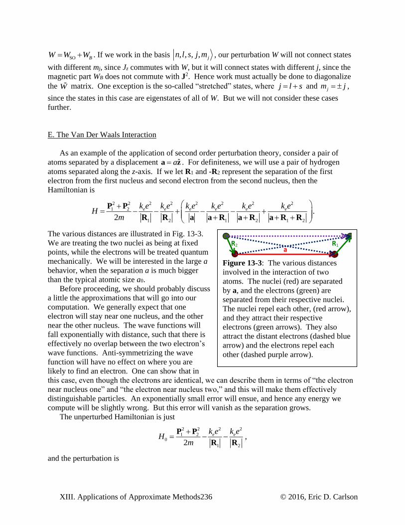
XIII. Applications of Approximate Methods236 © 2016, Eric D. Carlson
SO BW W W . If we work in the basis , , , , jn l s j m , our perturbation W will not connect states
with different mj, since Jz commutes with W, but it will connect states with different j, since the
magnetic part WB does not commute with J2. Hence work must actually be done to diagonalize
the W matrix. One exception is the so-called “stretched” states, where j l s and jm j ,
since the states in this case are eigenstates of all of W. But we will not consider these cases
further.
E. The Van Der Waals Interaction
As an example of the application of second order perturbation theory, consider a pair of
atoms separated by a displacement ˆaa z . For definiteness, we will use a pair of hydrogen
atoms separated along the z-axis. If we let R1 and -R2 represent the separation of the first
electron from the first nucleus and second electron from the second nucleus, then the
Hamiltonian is
2 2 2 2 2 22 2
1 2
1 2 1 2 1 2
.2
e e e e e ek e k e k e k e k e k eH
m
P P
R R a a R a R a R R
The various distances are illustrated in Fig. 13-3.
We are treating the two nuclei as being at fixed
points, while the electrons will be treated quantum
mechanically. We will be interested in the large a
behavior, when the separation a is much bigger
than the typical atomic size a0.
Before proceeding, we should probably discuss
a little the approximations that will go into our
computation. We generally expect that one
electron will stay near one nucleus, and the other
near the other nucleus. The wave functions will
fall exponentially with distance, such that there is
effectively no overlap between the two electron’s
wave functions. Anti-symmetrizing the wave
function will have no effect on where you are
likely to find an electron. One can show that in
this case, even though the electrons are identical, we can describe them in terms of “the electron
near nucleus one” and “the electron near nucleus two,” and this will make them effectively
distinguishable particles. An exponentially small error will ensue, and hence any energy we
compute will be slightly wrong. But this error will vanish as the separation grows.
The unperturbed Hamiltonian is just
2 22 2
1 20
1 2
,2
e ek e k eH
m
P P
R R
and the perturbation is
Figure 13-3: The various distances
involved in the interaction of two
atoms. The nuclei (red) are separated
by a, and the electrons (green) are
separated from their respective nuclei.
The nuclei repel each other, (red arrow),
and they attract their respective
electrons (green arrows). They also
attract the distant electrons (dashed blue
arrow) and the electrons repel each
other (dashed purple arrow).
R2 R1 a
© 2016, Eric D. Carlson 237 XIII. Applications of Approximate Methods
2 2 2 2
1 2 1 2
.e e e ek e k e k e k eW
a a R a R a R R (13.15)
The remaining terms will be treated as a perturbation; however, before we evaluate them, we
would like to approximate them. We expect that Ri will be small compared to a, so we can
expand the distances in powers of iR a . Choosing ˆaa z , and expanding to second order in
Ri, you can see that
121
22 2 2
2 2 2
2 2 2
1 1 2 1 31 1 .
2 2
Z Z Za Z X Y
a a a a a a a
R R
a R
Substituting this into Eq. (13.15) and simplifying, we find
2 22 2 2 21 2 1 21 1 1 2 2 2 1 2
2 2 2
2 3 2 311 2 1 2 1 2 1 2 1 22
33 31 1 1 1
2 2 2
6 2 2 .
e
e
e e
Z Zk e Z Z Z Z Z ZW
a a a a a a a
k e a Z Z k e a Z Z X X YY
R RR R
R R
We now wish to perform second-order perturbation theory on the ground state energy. The
unperturbed wave functions look like ;nlm n l m , and have unperturbed energies n n . The
first order perturbation to the ground state looks like
2 2 22 3100;100 100;100 2 100 100 100 100 100 100 .g eW k e a Z X Y
However, all of these matrix elements vanish, because matrix elements of the form
nlm n l m R vanish unless 1l l , as proven in chapter 7. Hence we must go to second
order, and we have
2
; 1
1; 100;100
2g
nlm n l m n n
nlm n l m W
(13.16)
Only 1l l contributes in this sum. This expression is unfortunately very difficult to
calculate, but we can get useful lower and upper bounds on its value. Because we are working
with the ground state, the denominator is always negative, and therefore any finite sum will give
us an overestimate of the energy. Let us consider only the lowest possible energy, which occurs
for 2n n . Consider, for example, the 1 2Z Z contribution, which, since it commutes with Lz,
is non-vanishing only when 0m m . Indeed, for this term in the sum, it is the only
contribution, and we find
22 3 2 3
1 2
5 2 2 3809
210;210 100;100 2 210;210 100;100 2 210 100
2 .
e e
e
W k e a Z Z k e a Z
a k e a
This term alone turns out to contribute two-thirds of the 2n n contribution to Eq. (13.16), so
that the contribution from 2n n yields the upper bound
XIII. Applications of Approximate Methods238 © 2016, Eric D. Carlson
10 10 102 4 4 2 4 4 2 5 2 50 0 0 0
6 6 66 2 21 2 0 0
4 1 1 6 8 2.468 8 8
2 2 9 9 94
e e e eg
e e
k e a k e a k e a k e a
a a aa k e a k e a
(13.17)
We can also use Eq. (13.16) to derive a lower limit on the ground state energy. When
deriving Eq. (13.17), we used Eq. (13.16), but treated the energy denominators as if they were all
infinite except for the lowest non-vanishing energy state 2n n . Of course, they are all
higher in energy, so for all the other states, we know that
1 2 12 2 2 .n n (13.18)
If we decrease all the denominators to this limiting value, we will be increasing the size of each
of these (negative) terms, and therefore obtain a lower bound on the energies. In fact, for the
bound states, the gap between the first excited state that contributes and all the other contributing
bound states is not much bigger, so replacing Eq. (13.18) with an equality will lead not only to a
lower bound, but probably a pretty good estimate. Substituting in Eq. (13.16), we obtain the
upper bound
2
2 2; ;1 2 0 0
; 100;100 100;100 ; ; 100;100,
2 2 4g
nlm n l m nlm n l m e e
nlm n l m W W nlm n l m nlm n l m W
k e a k e a
20
2
4100;100 100;100 ,
3g
e
aW
k e (13.19)
where in the last step, we used completeness of the intermediate states to perform the sum. We
now need to calculate
2 22 2 3
1 2 1 2 1 2100;100 100;100 100;100 2 100;100 .W ke a Z Z X X YY
Because of the high symmetry of the 1s state, cross terms like 1 2 1 2X X Z Z will have zero
expectation value. Hence all the cross terms will vanish, and the matrix elements we need will
be
2 2 4 6 2 2 2 2 2 2
1 2 1 2 1 2100;100 100;100 100;100 4 100;100eW k e a Z Z X X Y Y
2 2 22 4 6 2 2 24 100 100 100 100 100 100 .ek e a Z X Y (13.20)
Each of the matrix elements can then be calculated, and once again, due to symmetry, we expect
them to be all the same, so we have
0
2 2 2 213
2 20 2 2 2 3 4 21 40 10 0 03 30 0
100 100 100 100 100 100 100 100
, .r a
X Y Z
d Y r dr r R r a r e dr a
R
Substituting this into Eq. (13.20) and then Eq. (13.19) yields
2 5
0
6
8.e
g
k e a
a (13.21)
Comparing this with Eq. (13.17), we see that
© 2016, Eric D. Carlson 239 XIII. Applications of Approximate Methods
2 5
0
6,e
g
k e a
a
where 2.64 8 . We anticipate that the rather crude estimate Eq. (13.21) would not be as
good as Eq. (13.17), and indeed, a far more sophisticated analysis shows that 6.50 . This
new term represents an attractive potential between the two atoms for 0a a . This new
interaction is called the van der Waals interaction, and experimentally exhibits the behavior of
neutral atoms separated by large distances.
Of course, we have only demonstrated this a-6 behavior for hydrogen, but similar arguments
will apply in many other cases. In general, the matrix elements g gW will vanish, since the
ground state tends to have a definite value of l, which means that we always end up going to
second order. The second order contributions will always look like 2
gW , will be
attractive, and will come out like 2 5 6
0ek e a a , though the constant will depend on the type
of atom involved. If the first excited state is far above the ground state in energy, such as occurs
for a noble gas like helium, the energy denominator will tend to be large and the van der Waals
force small, whereas more reactive atoms will tend to have smaller energy denominators, and
feel a stronger long-range force.
Problems for Chapter 13
1. In section A we worked out the effect of the perturbation of the finite nuclear size assuming
the nucleus is a uniform sphere with radius a.
(a) Redo the calculation assuming instead that the nucleus is a spherical shell of radius a
with total charge e.
(b) Now, assume that the nucleus consists of two shells of radii a1 and a2, with charges q1
and q2 with e = q1 + q2. What is the shift due to the finite nuclear size in this case?
(c) Generalize part (b) to the case of N charges of magnitude qi at radii ai. Now generalize to
the case of continuous charge distribution q(r) which is normalized so q r dr e . No
proof is needed, but if you did part (b) correctly, the generalization should be obvious.
(d) For a uniform sphere of charge q and radius a, what is the charge density? What is the
charge q(r)dr in a thin spherical shell of radius r and thickness dr? Use this to find the
energy shift for a uniform sphere. Check it against the formula derived in class.
2. Complete the computation of the spin-orbit splitting for hydrogen for the 2p, 3p, and 3d
states of hydrogen. Write your answers as multiples of 2
nE , where is the fine structure
constant and nE is the unperturbed binding energy of this state.
3. Prove, as asserted in section C, that ˆ ˆ3 0j k jkr r d . This is nine equations, but only
six of them are independent.
4. We would like to know the hyperfine splitting for ordinary hydrogen 1H and deuterium 2H.
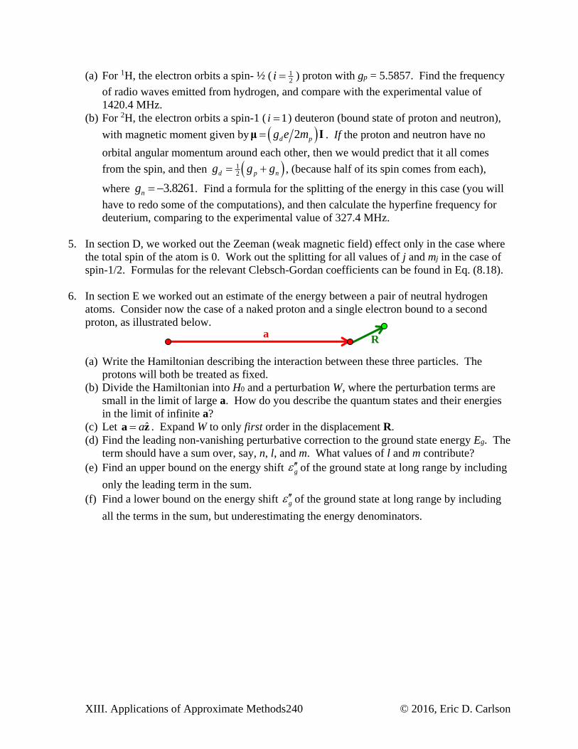
XIII. Applications of Approximate Methods240 © 2016, Eric D. Carlson
(a) For 1H, the electron orbits a spin- ½ ( 12
i ) proton with gp = 5.5857. Find the frequency
of radio waves emitted from hydrogen, and compare with the experimental value of
1420.4 MHz.
(b) For 2H, the electron orbits a spin-1 ( 1i ) deuteron (bound state of proton and neutron),
with magnetic moment given by 2d pg e mμ I . If the proton and neutron have no
orbital angular momentum around each other, then we would predict that it all comes
from the spin, and then 12d p ng g g , (because half of its spin comes from each),
where 3.8261ng . Find a formula for the splitting of the energy in this case (you will
have to redo some of the computations), and then calculate the hyperfine frequency for
deuterium, comparing to the experimental value of 327.4 MHz.
5. In section D, we worked out the Zeeman (weak magnetic field) effect only in the case where
the total spin of the atom is 0. Work out the splitting for all values of j and mj in the case of
spin-1/2. Formulas for the relevant Clebsch-Gordan coefficients can be found in Eq. (8.18).
6. In section E we worked out an estimate of the energy between a pair of neutral hydrogen
atoms. Consider now the case of a naked proton and a single electron bound to a second
proton, as illustrated below.
(a) Write the Hamiltonian describing the interaction between these three particles. The
protons will both be treated as fixed.
(b) Divide the Hamiltonian into H0 and a perturbation W, where the perturbation terms are
small in the limit of large a. How do you describe the quantum states and their energies
in the limit of infinite a?
(c) Let ˆaa z . Expand W to only first order in the displacement R.
(d) Find the leading non-vanishing perturbative correction to the ground state energy Eg. The
term should have a sum over, say, n, l, and m. What values of l and m contribute?
(e) Find an upper bound on the energy shift g of the ground state at long range by including
only the leading term in the sum.
(f) Find a lower bound on the energy shift g of the ground state at long range by including
all the terms in the sum, but underestimating the energy denominators.
a R
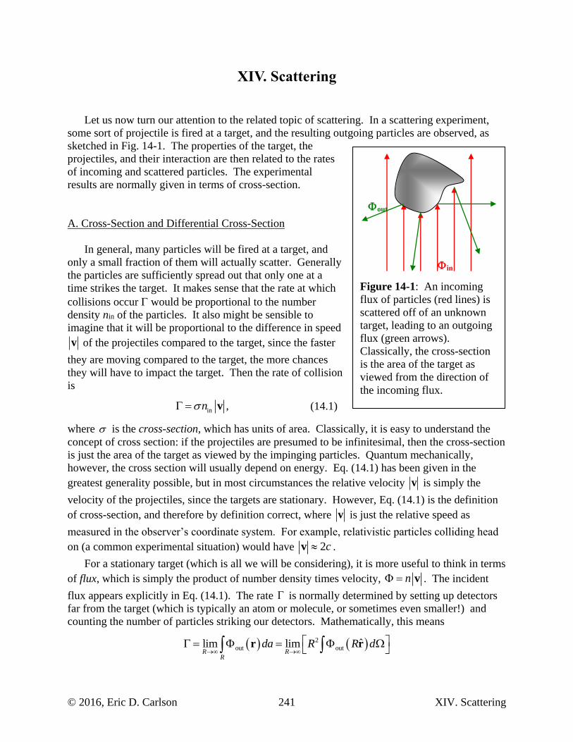
© 2016, Eric D. Carlson 241 XIV. Scattering
XIV. Scattering
Let us now turn our attention to the related topic of scattering. In a scattering experiment,
some sort of projectile is fired at a target, and the resulting outgoing particles are observed, as
sketched in Fig. 14-1. The properties of the target, the
projectiles, and their interaction are then related to the rates
of incoming and scattered particles. The experimental
results are normally given in terms of cross-section.
A. Cross-Section and Differential Cross-Section
In general, many particles will be fired at a target, and
only a small fraction of them will actually scatter. Generally
the particles are sufficiently spread out that only one at a
time strikes the target. It makes sense that the rate at which
collisions occur would be proportional to the number
density nin of the particles. It also might be sensible to
imagine that it will be proportional to the difference in speed
v of the projectiles compared to the target, since the faster
they are moving compared to the target, the more chances
they will have to impact the target. Then the rate of collision
is
in ,n v (14.1)
where is the cross-section, which has units of area. Classically, it is easy to understand the
concept of cross section: if the projectiles are presumed to be infinitesimal, then the cross-section
is just the area of the target as viewed by the impinging particles. Quantum mechanically,
however, the cross section will usually depend on energy. Eq. (14.1) has been given in the
greatest generality possible, but in most circumstances the relative velocity v is simply the
velocity of the projectiles, since the targets are stationary. However, Eq. (14.1) is the definition
of cross-section, and therefore by definition correct, where v is just the relative speed as
measured in the observer’s coordinate system. For example, relativistic particles colliding head
on (a common experimental situation) would have 2cv .
For a stationary target (which is all we will be considering), it is more useful to think in terms
of flux, which is simply the product of number density times velocity, n v . The incident
flux appears explicitly in Eq. (14.1). The rate is normally determined by setting up detectors
far from the target (which is typically an atom or molecule, or sometimes even smaller!) and
counting the number of particles striking our detectors. Mathematically, this means
2
out outˆlim lim
R RR
da R R d
r r
Figure 14-1: An incoming
flux of particles (red lines) is
scattered off of an unknown
target, leading to an outgoing
flux (green arrows).
Classically, the cross-section
is the area of the target as
viewed from the direction of
the incoming flux.
in
out
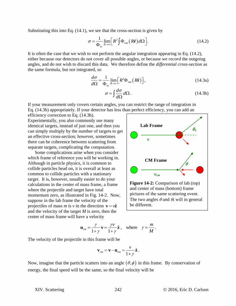
XIV. Scattering 242 © 2016, Eric D. Carlson
Substituting this into Eq. (14.1), we see that the cross-section is given by
2
out
in
1ˆlim .
RR R d
r (14.2)
It is often the case that we wish to not perform the angular integration appearing in Eq. (14.2),
either because our detectors do not cover all possible angles, or because we record the outgoing
angles, and do not wish to discard this data. We therefore define the differential cross-section as
the same formula, but not integrated, so
2
out
in
1ˆlim ,
R
dR R
d
r (14.3a)
.d
dd
(14.3b)
If your measurement only covers certain angles, you can restrict the range of integration in
Eq. (14.3b) appropriately. If your detector has less than perfect efficiency, you can add an
efficiency correction to Eq. (14.3b).
Experimentally, you also commonly use many
identical targets, instead of just one, and then you
can simply multiply by the number of targets to get
an effective cross-section; however, sometimes
there can be coherence between scattering from
separate targets, complicating the computation.
Some complications arise when you consider
which frame of reference you will be working in.
Although in particle physics, it is common to
collide particles head on, it is overall at least as
common to collide particles with a stationary
target. It is, however, usually easier to do your
calculations in the center of mass frame, a frame
where the projectile and target have total
momentum zero, as illustrated in Fig. 14-2. Now,
suppose in the lab frame the velocity of the
projectiles of mass m is v in the direction ˆvv z
and the velocity of the target M is zero, then the
center of mass frame will have a velocity
ˆ , where .1 1
cm
v m
M
u v z
The velocity of the projectile in this frame will be
ˆ .1
cm cm
v
v v u z
Now, imagine that the particle scatters into an angle , in this frame. By conservation of
energy, the final speed will be the same, so the final velocity will be
Figure 14-2: Comparison of lab (top)
and center of mass (bottom) frame
pictures of the same scattering event.
The two angles and L will in general
be different.
L
v
vcm
Lab Frame
CM Frame
© 2016, Eric D. Carlson 243 XIV. Scattering
ˆ ˆ ˆsin cos sin sin cos .1
cm
v
v x y z
If we now go back to the lab frame, the scattered velocity measured in the lab will be
ˆ ˆ ˆsin cos sin sin cos .1
cm cm
v
v v u x y z (14.4)
It is easy to see from Eq. (14.4) that the azimuthal angle , which can be found from the ratio of
the x- and y-components of the velocity, are the same in the lab and center of mass frame, so
L . However, the polar angle , which is found from the ratio of the xy-components and the
z-component, will be given in the lab frame by
2
sin costan , or equivalently, cos .
cos 1 2 cosL L
(14.5)
The rate at which particles scatter into a given angle, as defined by Eq. (14.1), must however be
the same for both, since time runs at the same rate in both frames,1 so that we must have
LLd d d d d d . Indeed, these must match not only if we integrate over all
angles, but indeed also if we integrate over restricted angles, provided we match the integration
range according to equation Eq. (14.5). It follows that
.L
L
d dd d
d d
Since solid angle is given by cosd d d , it follows that
3221 1 2 coscos
.cos 1 cos
L
L L
dd d d d d
d d d d d d
(14.6)
This allows us to relate the lab frame differential cross-section to the center of mass frame cross-
section. However, the total cross-section is identical in the two cases, L .
In quantum mechanics it is complicated to consider many particles at once, so to simplify, we
will study a single particle scattering off of a potential. What do we use for the flux? Flux is
particles per unit volume times velocity. For one particle, the particles per unit volume is just the
probability density * , which integrates to one for a normalized wave function, and the
classical analog of v is just the probability current j. This suggests that we make the
replacement in in j and out out j in Eq. (14.3a).
We now start to tackle the problem quantum mechanically. As argued in chapter 11 section
G, one can generally treat an arbitrary initial state as if it is an eigenstate of energy, but whose
energy is unknown. Therefore we need only study the case where we have an energy eigenstate
(and, in fact, most experiments try to measure that initial energy as well as possible). We
therefore are trying to solve Schrödinger’s time-independent equation, which takes the form
1 This argument gets more complicated when relativity is considered. However, it is still true that the total cross-
section remains the same.
XIV. Scattering 244 © 2016, Eric D. Carlson
2
2 ,2
E V
r r r r (14.7)
where V(r) is the potential from our target. We first define k and U(r) by
2
2 2
2 2and ,k E U V
r r (14.8)
then Eq. (14.7) becomes
2 2 .k U r r r (14.9)
We will think of U as being non-zero only in the immediate vicinity of the target, so that at large
radii, U(r) will be treated as zero. In fact, our results will be valid provided U(r) falls off fast
enough; one can show that it is only necessary that it fall faster than r-1.
In general, there will be an infinite number of linearly independent solutions of Eq. (14.9),
but we will only be interested in particular ones. Typically, the incoming wave will be coming
from a specific direction (normally chosen to be ˆz ). These incoming waves will take the form
eikz, an exact solution of Eq. (14.9) in the absence of the potential. We also expect there to be
outgoing waves. To understand these, let us write Eq. (14.9) in spherical coordinates, ignoring
the potential term, and keep only to order r-1, so we have
2
2
2
10 ,k r
r r
r r
which has solutions
, ,ikr
k
ef
r
r
However, we are only interested in outgoing waves, representing the scattered waves, which
have the plus sign. Adding to this the incoming wave, we anticipate at large r we will have
lim , ,ikr
ikz
kr
ee f
r
r (14.10)
where the first term represents the incoming wave, and the second the scattered wave. The
function ,kf is called the scattering amplitude.
We then calculate the two fluxes using j , working out the flux for the incoming wave in
Cartesian coordinates and the outgoing in spherical coordinates. For the latter we keep only the
leading order term, which is the radial part
*
in in in
2* * inout out out 2
Im Im ,
Im Im , , , .
ikz ikz
ikr ikr
k k k
ke e
z
e ef f f
r r r r
If we now substitute these into Eq. (14.3a), we find
© 2016, Eric D. Carlson 245 XIV. Scattering
2
, .k
df
d
(14.11)
Hence the problem of finding the cross section is reduced to that of finding the scattering
amplitude ,kf , defined by the large r limit of the wave function, Eq. (14.10).
One detail that should be mentioned: we never correctly normalized our wave function, and
indeed, plane waves cannot be normalized. Fortunately, any normalization factor that we
multiply the wave function by will not contribute, because it will cancel between the numerator
and the denominator, so this is not a concern.
B. The Born Approximation
We now proceed to attempt to find the solutions of Schrödinger’s Eq. (14.9), starting from a
plane wave initial state. Let’s imagine writing our total wave function in the form
.ikze r r (14.12)
Then substituting this into the left side of Eq. (14.9), and recalling that the first term is an exact
solution in the absence of a potential, we have
2 2 .k U r r r (14.13)
We’ll now imagine that the right hand side of Eq. (14.13) is known and attempt to solve for the
left side. We will use the method of Green’s functions. Imagine, at first, that the right side of
Eq. (14.13) were a delta function centered at the origin. Then we would have to solve the
equation
2 2 3 .k G r r (14.14)
To solve this, we first note that the problem is spherically symmetric, so we anticipate the
solution will be spherically symmetrical: G G rr . Then, working in spherical coordinates,
Eq. (14.14) becomes
2
2 3
2
1.k G r rG r
r r
r
Away from the origin, the solution to this equation is ikrG r e r . But we are interested in an
outgoing wave, not an incoming, so we pick the plus sign, and we assume
.ikre
G rr
(14.15)
To determine the constant , substitute this formula into equation Eq. (14.14) and integrate over
a small spherical volume of radius a, using Gauss’s Law Eq. (A.19) for the Laplacian term, and
Eq. (A.12j) for the other term . We have
XIV. Scattering 246 © 2016, Eric D. Carlson
3 2 2 3 2 3 2
0
1 22 1 2
0
ˆ1 4
4 4 4 e 1 ,
a
ikr
V V V S
aikr ikr ika ika ika ika
rr a
d k G d G k d G dA G k re dr
da r e k ik r ik e ikae e ika e
dr
r r r r r r r r
1 4 .
Solving for and substituting into Eq. (14.15) and then Eq. (14.14), we have
2 2 3 .4
ikrek
r
r
We now have a solution to Eq. (14.13) if the right hand side is a delta-function centered at
the origin. Obviously, this problem is translation invariant, so we can make the source centered
anywhere if we replace r with r r :
2 2 3 ,4
ike
k
r r
r rr r
(14.16)
where the Laplacian 2 is understood to be with respect to r, not r . Now that we have the
solution to Eq. (14.13) for a point source at an arbitrary location, we need only use superposition
to find the solution for an arbitrary source. We multiply Eq. (14.16) by U r r on the
right, and then integrate over r to obtain
3 2 2 3 3 ,4
ike
d k U d U U
r r
r r r r r r r r r rr r
Comparison with Eq. (14.13) makes it clear that we have found an integral solution to
Eq. (14.13); namely, r is simply the integral given above, and substituting this into
Eq. (14.12) then tells us
3 .4
ik
ikz U ee d
r r
rr r r
r r (14.17)
Naively, it looks like we haven’t accomplished much, since Eq. (14.17) tells us that we can
find the wave function if we know the wave function. But this appearance is deceptive. Imagine
substituting the whole expression on the right side of Eq. (14.17) into itself, so that we obtain
3 3 3 .4 4 4
ik ik ik
ikz ikzU e U e U ee d e d d
r r r r r rr r r
r r r r rr r r r r r
This process can be repeated as many times as necessary, for example
3 3 3
4 4 4
ik ik ik
ikz ikz ikzU e U e U ee d e d d e
r r r r r rr r r
r r r rr r r r r r
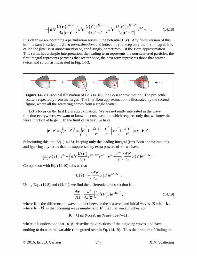
© 2016, Eric D. Carlson 247 XIV. Scattering
3 3 3 .
4 4 4
ik ik ik
ikzU e U e U ed d d e
r r r r r rr r r
r r rr r r r r r
(14.18)
It is clear we are obtaining a perturbation series in the potential U(r). Any finite version of this
infinite sum is called the Born approximation, and indeed, if you keep only the first integral, it is
called the first Born approximation or, confusingly, sometimes just the Born approximation.
This series has a simple interpretation: the leading term represents the non-scattered particles, the
first integral represents particles that scatter once, the next term represents those that scatter
twice, and so on, as illustrated in Fig. 14-3.
Let’s focus on the first Born approximation. We are not really interested in the wave
function everywhere, we want to know the cross-section, which requires only that we know the
wave function at large r. In the limit of large r, we have
2
2 2
2 2 2
2ˆ1 1 .r r r
r r r
r r r r rr r r r r r
Substituting this into Eq. (14.18), keeping only the leading integral (first Born approximation),
and ignoring any terms that are suppressed by extra powers of 1r we have
3ˆ ˆ3lim .
4 4
ikrik rikz ikz ikz ikz ik
r
U e de d e e e U e
r r
r r r rr r
r r r
Comparison with Eq. (14.10) tells us that
3
ˆˆ .4
ikz ik
k
df U e
r rrr r
Using Eqs. (14.8) and (14.11), we find the differential cross-section is
2 2
3
2 4,
4
idd V e
d
K rr r (14.19)
where K is the difference in wave number between the scattered and initial waves, K k k ,
where ˆkk z is the incoming wave number and k the final wave number, so
sin cos ,sin sin ,cos 1 ,k K
where it is understood that , describe the directions of the outgoing waves, and have
nothing to do with the variable r integrated over in Eq. (14.19). Thus the problem of finding the
Figure 14-3: Graphical illustration of Eq. (14.18), the Born approximation. The projectile
scatters repeatedly from the target. The first Born approximation is illustrated by the second
figure, where all the scattering comes from a single scatter.
+ + + +
XIV. Scattering 248 © 2016, Eric D. Carlson
differential cross-section has been reduced to simply that of finding the Fourier transform of the
potential.
Let’s illustrate the use of Eq. (14.19) for the Yukawa potential, given by
.rV er
r (14.20)
The first step is to find the Fourier transform of this potential, which is given by
3 3 1 .i r id V e d r e K r K rr r r
In this expression, we can pick our z-axis for the integration to be any axis we want, so to
simplify, pick it in the direction of K. Then the Fourier transform can be computed using
Eqs. (A.12h) and (A.13d) and becomes
1 2cos 1
3 2 1 cos cos
cos 10 1 0 0
2 2
0
1cos 2
2 2 1 1 4.
i r iKr r iKr
r iKr r iKr
d V e r r dr e d d rdr eiKr
i idr e e
K K iK iK
K rr r
K
It is easy to see that 22 22 1 cosk K k k , so we have
22 2 2
22 4 2 2 4 2 2 2
4 4.
4 2 1 cos 2 2 cos
d
d k k k
(14.21)
The total cross section can be computed with the help of Eqs. (A.12d) and is given by
12 2 2 2 2 2
24 4 2 2 2 2 4 2 2 22 2 21
8 cos 4 1 1 16.
4 42 2 cos
d dd
d k k kk k
Of particular interest to us is the case of Coulomb scattering, for which C eV k qq rr ,
where ke is Coulomb’s constant. This is a special case of Eq. (14.20), so we immediately find
the differential cross-section from Eq. (14.21). We have
2 2 2 2
24 4.
1 cos
C ed k q q
d k
If we use the formula for momentum, k v , we can write this in the more convenient form
2 2 2 2 2 2
2 2 4 4 12 42
.4 sin1 cos
C e ed k q q k q q
d vv
(14.22)
Note that the velocity in Eq. (14.22) is the relative velocity, and is the reduced mass. The
differential cross-section is then given in the center of mass frame. If the mass of the target is
not large compared to the projectile, you would then have to use Eqs. (14.5) and (14.6) to
transform it to the lab frame, a messy proposition.
© 2016, Eric D. Carlson 249 XIV. Scattering
Of some concern might be that we have assumed a potential that falls off as a sufficiently
strong power of r such that our waves can be assumed to asymptotically reach a region where we
can ignore the effect of the potential. This turns out not to be the case for the Coulomb potential.
The r-1 potential causes the wave to continue oscillating at large r in such a way that our
solutions are not really right, but instead have an additional distance-dependant phase shift.
Fortunately, this shift in only the phase of the wave does not affect the probabilities. We have
obscured this problem by treating the Coulomb potential as the limiting case of the Yukawa
potential, but if you reexamine the steps leading to Eq. (14.21), you will see that problems arise
if = 0. Nonetheless, it is known that Eq. (14.22) is correct; indeed, it is known to be not only
correct in the first Born approximation, but in fact always exact1.
The total Coulomb cross-section is in fact infinite, which can be seen by integrating
Eq. (14.22). The problem is small angles, where the differential cross-section blows up. This
just represents an effect of the long-range interaction. No matter how far off-axis the incoming
projectile is, it will always be deflected a tiny bit by this long-range force. Experimentally, the
measured cross-section will always be finite, because there is some minimum angle min that can
be experimentally distinguished from zero. This effectively introduces a cutoff in our
integration, yielding an experimentally finite cross-section.
C. Scattering from a Spherically Symmetric Potential
One of the most common situations we are interested in is scattering from a spherically
symmetric potential. In such cases, we know that the solutions of the Schrödinger equation take
on the form of spherical harmonics times radial wave functions, so we suspect we can find
solutions of Eq. (14.9) of the form
, .m
lm l lR r Y r (14.23)
We will analyze these waves one at a time for each value of l and m; so that this method is called
the method of partial waves. If we substitute this into Eq. (14.9) and use the fact that the angular
part of the spherical Laplacian in spherical coordinates Eq. (A.32d) can be written in terms of the
angular momentum operator L2 using Eq. (7.23), we find
2 2
2
2 2 2
1, , , , ,m m m m
l l l l l l l lk R r Y rR r Y R r Y U r R r Yr r r
L
2 2
2
2 2
1.l l
d l lrR r U r k R r
r dr r
(14.24)
The differential Eq. (14.24) must be solved subject to appropriate boundary conditions.
Let us solve Eq. (14.24) in two extreme cases, when r is very small, and when it is very large.
For small r, the angular momentum term will tend to dominate, so we have
1 Well, exact if we ignore relativistic corrections, radiative corrections (which come from quantizing the
electromagnetic field), internal structure of the projectile or target, magnetic interactions, and so on. No realistic
calculation is ever really exact.
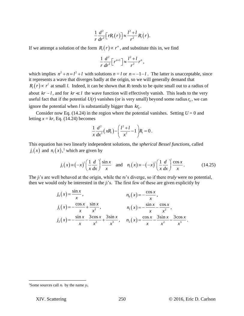
XIV. Scattering 250 © 2016, Eric D. Carlson
2 2
2 2
1.l l
d l lrR r R r
r dr r
If we attempt a solution of the form n
lR r r , and substitute this in, we find
2 2
1
2 2
1,n nd l l
r rr dr r
which implies 2 2n n l l with solutions n = l or 1n l . The latter is unacceptable, since
it represents a wave that diverges badly at the origin, so we will generally demand that
l
lR r r at small l. Indeed, it can be shown that Rl tends to be quite small out to a radius of
about kr l , and for kr l the wave function will effectively vanish. This leads to the very
useful fact that if the potential U(r) vanishes (or is very small) beyond some radius0r , we can
ignore the potential when l is substantially bigger than 0kr .
Consider now Eq. (14.24) in the region where the potential vanishes. Setting U = 0 and
letting x = kr, Eq. (14.24) becomes
2 2
2 2
11 0 .l l
d l lxR R
x dx x
This equation has two linearly independent solutions, the spherical Bessel functions, called
lj x and ln x ,1 which are given by
1 sin 1 cos
and .
l ll l
l l
d x d xj x x n x x
x dx x x dx x
(14.25)
The jl’s are well behaved at the origin, while the nl’s diverge, so if there truly were no potential,
then we would only be interested in the jl’s. The first few of these are given explicitly by
0
1 2
2 2 3
sin,
cos sin,
sin 3cos 3sin,
xj x
x
x xj x
x x
x x xj x
x x x
0
1 2
2 2 3
cos,
sin cos,
cos 3sin 3cos.
xn x
x
x xn x
x x
x x xn x
x x x
1Some sources call nl by the name yl.
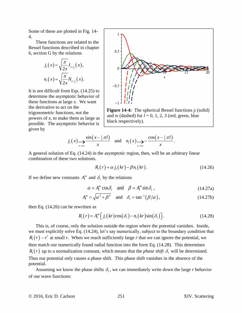
© 2016, Eric D. Carlson 251 XIV. Scattering
Some of these are plotted in Fig. 14-
4.
These functions are related to the
Bessel functions described in chapter
6, section G by the relations
12
12
,2
.2
l l
l l
j x J xx
n x N xx
It is not difficult from Eqs. (14.25) to
determine the asymptotic behavior of
these functions at large x. We want
the derivative to act on the
trigonometric functions, not the
powers of x, to make them as large as
possible. The asymptotic behavior is
given by
1 1
2 2sin cosand .l l
x x
x l x lj x n x
x x
A general solution of Eq. (14.24) in the asymptotic region, then, will be an arbitrary linear
combination of these two solutions.
.l l lR r j kr n kr (14.26)
If we define new constants m
lA and l by the relations
cos and sin ,m m
l l l lA A (14.27a)
2 2 1and tan ,m
l lA (14.27b)
then Eq. (14.26) can be rewritten as
cos sin .m
l l l l l lR r A j kr n kr (14.28)
This is, of course, only the solution outside the region where the potential vanishes. Inside,
we must explicitly solve Eq. (14.24), let’s say numerically, subject to the boundary condition that
l
lR r r at small r. When we reach sufficiently large r that we can ignore the potential, we
then match our numerically found radial function into the form Eq. (14.28). This determines
lR r up to a normalization constant, which means that the phase shift l will be determined.
Thus our potential only causes a phase shift. This phase shift vanishes in the absence of the
potential.
Assuming we know the phase shifts l , we can immediately write down the large r behavior
of our wave functions:
Figure 14-4: The spherical Bessel functions jl (solid)
and nl (dashed) for l = 0, 1, 2, 3 (red, green, blue
black respectively).
XIV. Scattering 252 © 2016, Eric D. Carlson
1 12 2
, cos sin ,
sin cos cos sin , ,
m m m
l l l l l l l l
mml
l l lr
R r Y A j kr n kr Y
Akr l kr l Y
kr
r
12
1sin , .m m
l l lr
A kr l Ykr
r (14.29)
We have successfully solved Eq. (14.28), but we seem to be no closer to finding the cross-
section. To clarify the problem, write out Eq. (14.29) in terms of exponentials, so we have
1 12 2
exp exp , .2
mml
l l lr
Aikr i l i ikr i l i Y
ikr
r
,
1, .
2l li im l ikr l ikr m
l lr l m
A i e e i e e Yikr
r (14.30)
This clearly consists of two waves, an incoming and an outgoing wave, but the incoming wave is
coming from all directions (or at least, most directions), not just the z-direction. The key to
getting this to work out is to take linear combinations of Eq. (14.30), choosing constants m
lA in
such a way to turn the second incoming wave into one of the form cosikz ikre e . Our goal is to
cleverly choose m
lA in such a way that we recognize the sum as a term that goes like cosikre ,
added to a term that looks like an outgoing wave. To assist us, we need to write cosikre as a sum
of spherical harmonics. This can always be done, so we are trying to find constants m
lc r
(functions of r), such that
cos
,
, .m m ikr
l l
l m
c r Y e (14.31)
To do so, we will use the orthonormality of the Y’s, so that
*
, exp cos .m m
l lc r d Y ikr
The integral is easy to do, since the m
lY ’s always go as ime . The result vanishes unless m = 0,
and for m = 0 we have
1
*0 0 cos
1
2 cos , .ikr
l lc r d Y e
We are interested in the large r behavior, so we integrate this by parts to yield
0* *0 0 cos cos 0
* *0 0 2
2 2, cos ,
cos
20, , .
ikr ikr
l l l
ikr ikr
l l
dc r Y e d e Y
ikr ikr d
e Y e Y O rikr
The upper limit can be found in equation Eq. (8.36), and Eq. (7.33) helps you get the lower limit,
so
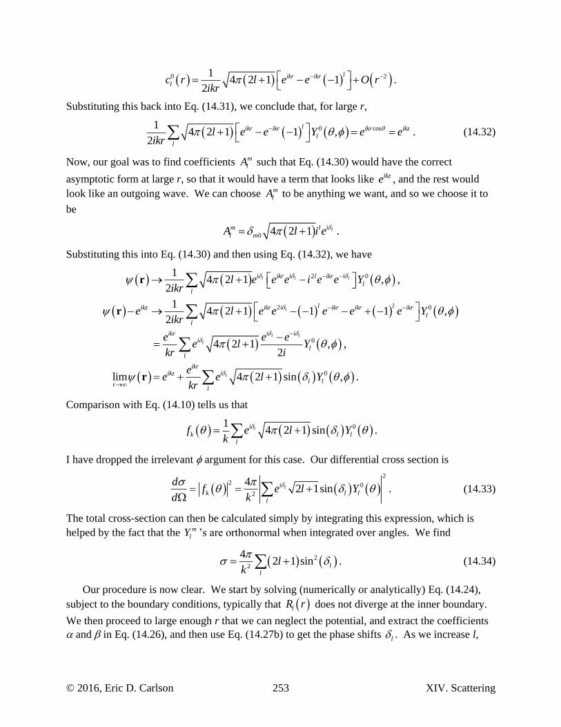
© 2016, Eric D. Carlson 253 XIV. Scattering
0 214 2 1 1 .
2
likr ikr
lc r l e e O rikr
Substituting this back into Eq. (14.31), we conclude that, for large r,
0 cos14 2 1 1 , .
2
likr ikr ikr ikz
l
l
l e e Y e eikr
(14.32)
Now, our goal was to find coefficients m
lA such that Eq. (14.30) would have the correct
asymptotic form at large r, so that it would have a term that looks like ikze , and the rest would
look like an outgoing wave. We can choose m
lA to be anything we want, and so we choose it to
be
0 4 2 1 .lim l
l mA l i e
Substituting this into Eq. (14.30) and then using Eq. (14.32), we have
2 0
2 0
0
0
14 2 1 , ,
2
14 2 1 1 1 ,
2
4 2 1 , ,2
lim 4 2 1 sin , .
l l l
l
l l
l
l
i i iikr l ikr
l
l
l liikz ikr ikr ikr ikr
l
l
i iikri
l
l
ikriikz
l lr
l
l e e e i e e Yikr
e l e e e e e Yikr
e e ee l Y
kr i
ee e l Y
kr
r
r
r
Comparison with Eq. (14.10) tells us that
014 2 1 sin .li
k l l
l
f e l Yk
I have dropped the irrelevant argument for this case. Our differential cross section is
2
2 0
2
42 1sin .li
k l l
l
df e l Y
d k
(14.33)
The total cross-section can then be calculated simply by integrating this expression, which is
helped by the fact that the m
lY ’s are orthonormal when integrated over angles. We find
2
2
42 1 sin .l
l
lk
(14.34)
Our procedure is now clear. We start by solving (numerically or analytically) Eq. (14.24),
subject to the boundary conditions, typically that lR r does not diverge at the inner boundary.
We then proceed to large enough r that we can neglect the potential, and extract the coefficients
and in Eq. (14.26), and then use Eq. (14.27b) to get the phase shifts l . As we increase l,
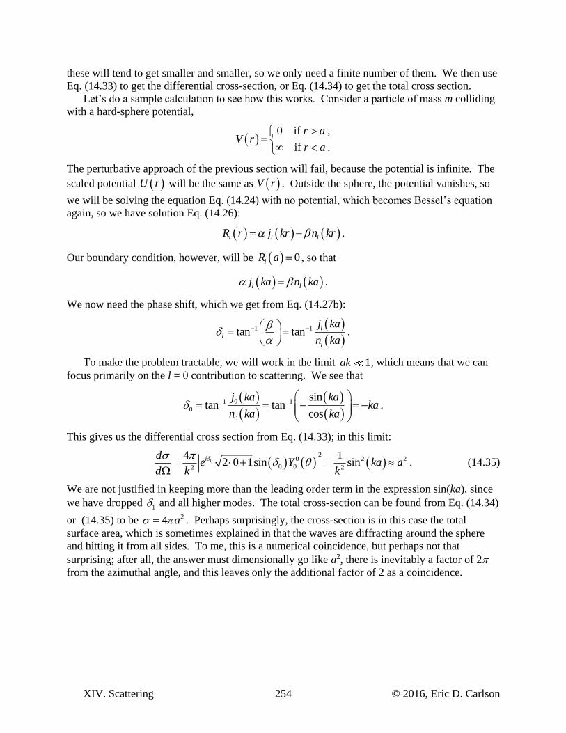
XIV. Scattering 254 © 2016, Eric D. Carlson
these will tend to get smaller and smaller, so we only need a finite number of them. We then use
Eq. (14.33) to get the differential cross-section, or Eq. (14.34) to get the total cross section.
Let’s do a sample calculation to see how this works. Consider a particle of mass m colliding
with a hard-sphere potential,
0 if ,
if .
r aV r
r a
The perturbative approach of the previous section will fail, because the potential is infinite. The
scaled potential U r will be the same as V r . Outside the sphere, the potential vanishes, so
we will be solving the equation Eq. (14.24) with no potential, which becomes Bessel’s equation
again, so we have solution Eq. (14.26):
.l l lR r j kr n kr
Our boundary condition, however, will be 0lR a , so that
.l lj ka n ka
We now need the phase shift, which we get from Eq. (14.27b):
1 1tan tan .l
l
l
j ka
n ka
To make the problem tractable, we will work in the limit 1ak , which means that we can
focus primarily on the l = 0 contribution to scattering. We see that
01 1
0
0
sintan tan .
cos
j ka kaka
n ka ka
This gives us the differential cross section from Eq. (14.33); in this limit:
0
20 2 2
0 02 2
4 12 0 1sin sin .id
e Y ka ad k k
(14.35)
We are not justified in keeping more than the leading order term in the expression sin(ka), since
we have dropped 1 and all higher modes. The total cross-section can be found from Eq. (14.34)
or (14.35) to be 24 a . Perhaps surprisingly, the cross-section is in this case the total
surface area, which is sometimes explained in that the waves are diffracting around the sphere
and hitting it from all sides. To me, this is a numerical coincidence, but perhaps not that
surprising; after all, the answer must dimensionally go like a2, there is inevitably a factor of 2
from the azimuthal angle, and this leaves only the additional factor of 2 as a coincidence.
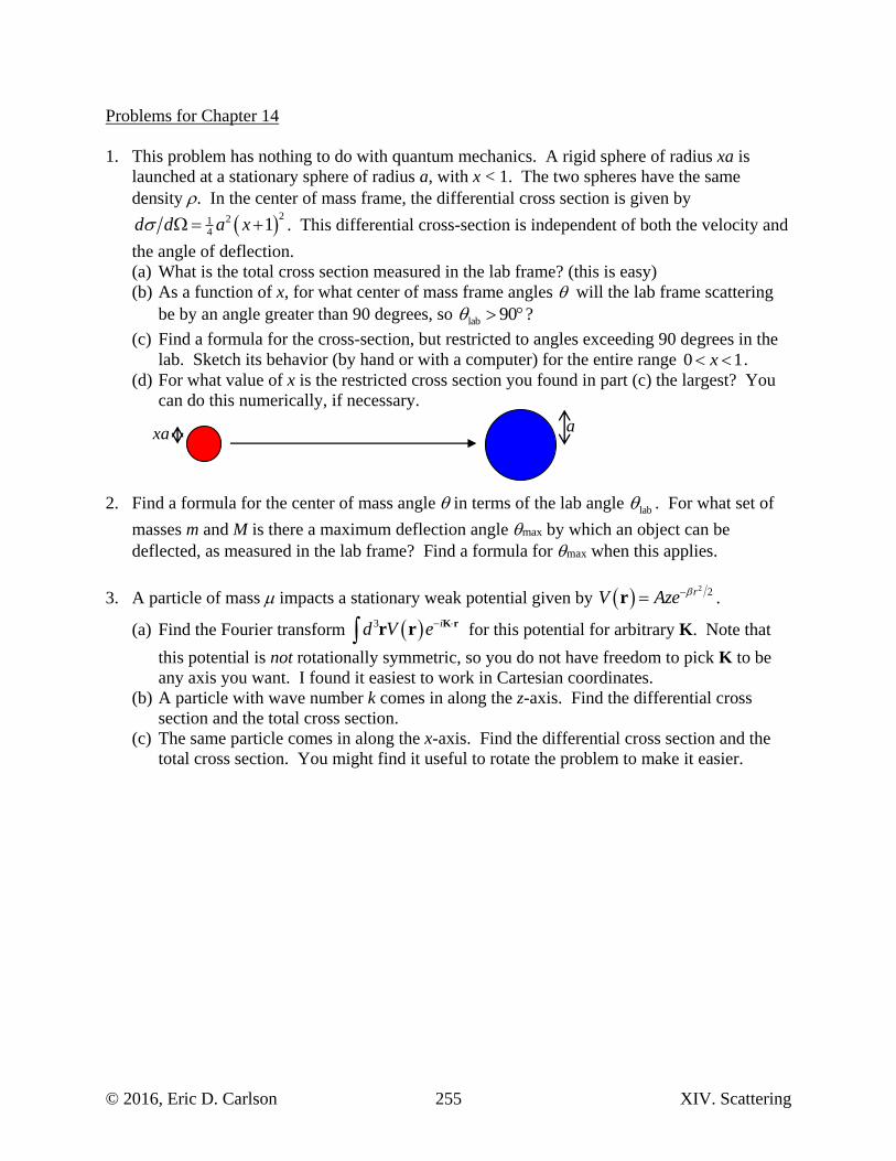
© 2016, Eric D. Carlson 255 XIV. Scattering
Problems for Chapter 14
1. This problem has nothing to do with quantum mechanics. A rigid sphere of radius xa is
launched at a stationary sphere of radius a, with x < 1. The two spheres have the same
density . In the center of mass frame, the differential cross section is given by
221
41d d a x . This differential cross-section is independent of both the velocity and
the angle of deflection.
(a) What is the total cross section measured in the lab frame? (this is easy)
(b) As a function of x, for what center of mass frame angles will the lab frame scattering
be by an angle greater than 90 degrees, so lab 90 ?
(c) Find a formula for the cross-section, but restricted to angles exceeding 90 degrees in the
lab. Sketch its behavior (by hand or with a computer) for the entire range 0 1x .
(d) For what value of x is the restricted cross section you found in part (c) the largest? You
can do this numerically, if necessary.
2. Find a formula for the center of mass angle in terms of the lab angle lab . For what set of
masses m and M is there a maximum deflection angle max by which an object can be
deflected, as measured in the lab frame? Find a formula for max when this applies.
3. A particle of mass impacts a stationary weak potential given by 2 2rV Aze r .
(a) Find the Fourier transform 3 id V e
K rr r for this potential for arbitrary K. Note that
this potential is not rotationally symmetric, so you do not have freedom to pick K to be
any axis you want. I found it easiest to work in Cartesian coordinates.
(b) A particle with wave number k comes in along the z-axis. Find the differential cross
section and the total cross section.
(c) The same particle comes in along the x-axis. Find the differential cross section and the
total cross section. You might find it useful to rotate the problem to make it easier.
xa a
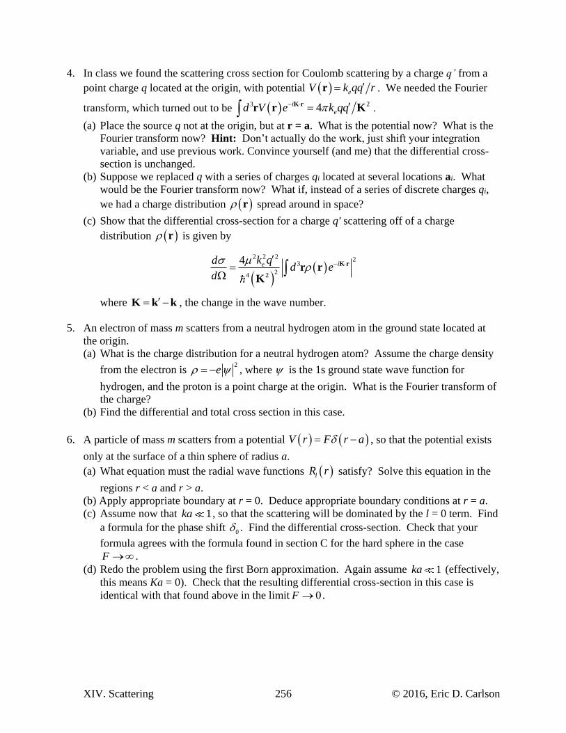
XIV. Scattering 256 © 2016, Eric D. Carlson
4. In class we found the scattering cross section for Coulomb scattering by a charge q’ from a
point charge q located at the origin, with potential eV k qq rr . We needed the Fourier
transform, which turned out to be 3 24i
ed V e k qq K rr r K .
(a) Place the source q not at the origin, but at r = a. What is the potential now? What is the
Fourier transform now? Hint: Don’t actually do the work, just shift your integration
variable, and use previous work. Convince yourself (and me) that the differential cross-
section is unchanged.
(b) Suppose we replaced q with a series of charges qi located at several locations ai. What
would be the Fourier transform now? What if, instead of a series of discrete charges qi,
we had a charge distribution r spread around in space?
(c) Show that the differential cross-section for a charge q' scattering off of a charge
distribution r is given by
2 2 2 23
24 2
4 iek qdd e
d
K rr rK
where K k k , the change in the wave number.
5. An electron of mass m scatters from a neutral hydrogen atom in the ground state located at
the origin.
(a) What is the charge distribution for a neutral hydrogen atom? Assume the charge density
from the electron is 2
e , where is the 1s ground state wave function for
hydrogen, and the proton is a point charge at the origin. What is the Fourier transform of
the charge?
(b) Find the differential and total cross section in this case.
6. A particle of mass m scatters from a potential V r F r a , so that the potential exists
only at the surface of a thin sphere of radius a.
(a) What equation must the radial wave functions lR r satisfy? Solve this equation in the
regions r < a and r > a.
(b) Apply appropriate boundary at r = 0. Deduce appropriate boundary conditions at r = a.
(c) Assume now that 1ka , so that the scattering will be dominated by the l = 0 term. Find
a formula for the phase shift 0 . Find the differential cross-section. Check that your
formula agrees with the formula found in section C for the hard sphere in the case
F .
(d) Redo the problem using the first Born approximation. Again assume 1ka (effectively,
this means Ka = 0). Check that the resulting differential cross-section in this case is
identical with that found above in the limit 0F .


![[PPT]No Slide Titleusers.wfu.edu/ecarlson/phy114/lectures/emwaves.ppt · Web viewElectromagnetic Waves Wave Solutions Maxwell’s Equations, no sources: Changing E-flux creates B-field](https://img.pdfslide.us/doc/110x75/5aa9b1b37f8b9a90188d2f61/pptno-slide-viewelectromagnetic-waves-wave-solutions-maxwells-equations-no.jpg)


![[PPT]No Slide Title - Wake Forest Student, Faculty and Staff …ecarlson/astro/lectures/... · Web viewTitle No Slide Title Author Wake Forest University Last modified by Carlson,](https://img.pdfslide.us/doc/110x75/5af1473f7f8b9ac57a8fae7d/pptno-slide-title-wake-forest-student-faculty-and-staff-ecarlsonastrolecturesweb.jpg)


![Xi How to Integrate Bw to Xi[1]](https://img.pdfslide.us/doc/110x75/577d23681a28ab4e1e99b43b/xi-how-to-integrate-bw-to-xi1.jpg)


![Paper Class XI[Nurture(X-XI)]](https://img.pdfslide.us/doc/110x75/55cf93c3550346f57b9e4fc8/paper-class-xinurturex-xi.jpg)