XFDTDcfurse/Tutorials/XFDTD/man50492.pdf7 1-2-2 Define Project Parameters Once the geometry is defined, the FDTD calculation parameters for the specific project are chosen. These parameters

REMCOM, Inc. Calder Square P.O. Box 10023 State College, PA 16805

Phone (814) 353-2986Fax (814) 353-1420e-mail [email protected] http://www.remcom.com

USER’S MANUAL

FOR

XFDTDTHE

FINITE DIFFERENCE TIME DOMAIN

GRAPHICAL USER INTERFACE

FOR

ELECTROMAGNETIC CALCULATIONS

Version 5.0.4.9

Sept 1999

Copyright © 1994-1999 REMCOM, Inc.All Rights Reserved

XFDTD® is a Registered Trademark of Remcom, Inc.

2

Table of Contents

1 Introduction . . . . . . . . . . . . . . . . . . . . . . . . . . . . . . . . . . . . . . . . . . . . . . . . . . . . . . . . 61-1 Operating System . . . . . . . . . . . . . . . . . . . . . . . . . . . . . . . . . . . . . . . . . . . . 61-2 General Technique for FDTD Calculations . . . . . . . . . . . . . . . . . . . . . . . . . 6

1-2-1 Define Geometry . . . . . . . . . . . . . . . . . . . . . . . . . . . . . . . . . . . . . . 61-2-2 Define Project Parameters . . . . . . . . . . . . . . . . . . . . . . . . . . . . . . 71-2-3 Results and Output . . . . . . . . . . . . . . . . . . . . . . . . . . . . . . . . . . . . 7

1-3 Summary of XFDTD Features . . . . . . . . . . . . . . . . . . . . . . . . . . . . . . . . . . . 7

2 Installation and Licensing . . . . . . . . . . . . . . . . . . . . . . . . . . . . . . . . . . . . . . . . . . . . 11

3 Estimating Computer Resource Requirements . . . . . . . . . . . . . . . . . . . . . . . . . . . 123-1 Defining the Cell Size . . . . . . . . . . . . . . . . . . . . . . . . . . . . . . . . . . . . . . . 12

3-1-1 Creating a Geometry with FDTD Cells . . . . . . . . . . . . . . . . . . . . . 123-1-2 Free Space Boundaries . . . . . . . . . . . . . . . . . . . . . . . . . . . . . . . . 13

3-2 Determining the Total Number of Cells . . . . . . . . . . . . . . . . . . . . . . . . . . . 133-3 Estimating the Necessary Computer Resources . . . . . . . . . . . . . . . . . . . 13

3-3-1 Far-Zone Radiation angles at a single frequency . . . . . . . . . . . . 143-3-2 Execution Time Estimation . . . . . . . . . . . . . . . . . . . . . . . . . . . . . 14

3-4 Coordinate System . . . . . . . . . . . . . . . . . . . . . . . . . . . . . . . . . . . . . . . . . . 16

4 XFDTD Graphical User Interface . . . . . . . . . . . . . . . . . . . . . . . . . . . . . . . . . . . . . . 174-1 Starting XFDTD . . . . . . . . . . . . . . . . . . . . . . . . . . . . . . . . . . . . . . . . . . . . . 17

4-1-1 Starting XFDTD in Windows NT/95/98 . . . . . . . . . . . . . . . . . . . . 174-1-2 Starting XFDTD in UNIX . . . . . . . . . . . . . . . . . . . . . . . . . . . . . . . 17

4-2 The XFDTD User Interface . . . . . . . . . . . . . . . . . . . . . . . . . . . . . . . . . . . . 17

5 File Types . . . . . . . . . . . . . . . . . . . . . . . . . . . . . . . . . . . . . . . . . . . . . . . . . . . . . . . . 235-1 Geometry Files . . . . . . . . . . . . . . . . . . . . . . . . . . . . . . . . . . . . . . . . . . . . . 235-2 Project Files . . . . . . . . . . . . . . . . . . . . . . . . . . . . . . . . . . . . . . . . . . . . . . . . 245-3 Output Files . . . . . . . . . . . . . . . . . . . . . . . . . . . . . . . . . . . . . . . . . . . . . . . . 24

6 The File Menu . . . . . . . . . . . . . . . . . . . . . . . . . . . . . . . . . . . . . . . . . . . . . . . . . . . . . 266-1 The File Menu in Windows NT/95/98 . . . . . . . . . . . . . . . . . . . . . . . . . . . . . 26

6-1-1 New . . . . . . . . . . . . . . . . . . . . . . . . . . . . . . . . . . . . . . . . . . . . . . . 266-1-2 Open . . . . . . . . . . . . . . . . . . . . . . . . . . . . . . . . . . . . . . . . . . . . . . 286-1-3 Merge . . . . . . . . . . . . . . . . . . . . . . . . . . . . . . . . . . . . . . . . . . . . . . 286-1-4 Save . . . . . . . . . . . . . . . . . . . . . . . . . . . . . . . . . . . . . . . . . . . . . . . 286-1-5 Save As . . . . . . . . . . . . . . . . . . . . . . . . . . . . . . . . . . . . . . . . . . . . 286-1-6 Close . . . . . . . . . . . . . . . . . . . . . . . . . . . . . . . . . . . . . . . . . . . . . . 296-1-7 Exit . . . . . . . . . . . . . . . . . . . . . . . . . . . . . . . . . . . . . . . . . . . . . . . . 29

6-2 The File Menu in UNIX XFDTD . . . . . . . . . . . . . . . . . . . . . . . . . . . . . . . . . 296-2-1 Open Geometry File . . . . . . . . . . . . . . . . . . . . . . . . . . . . . . . . . . 296-2-2 Open XFDTD Project File . . . . . . . . . . . . . . . . . . . . . . . . . . . . . . 306-2-3 Open Geometry File and Merge with Present Geometry . . . . . . . 30

3

6-2-4 Adjust Merge Characteristics . . . . . . . . . . . . . . . . . . . . . . . . . . . . 306-2-5 Open ... File . . . . . . . . . . . . . . . . . . . . . . . . . . . . . . . . . . . . . . . . . 316-2-6 Create New Space . . . . . . . . . . . . . . . . . . . . . . . . . . . . . . . . . . . . 316-2-7 Show Information Window . . . . . . . . . . . . . . . . . . . . . . . . . . . . . . 326-2-8 Save Geometry . . . . . . . . . . . . . . . . . . . . . . . . . . . . . . . . . . . . . . 326-2-9 Save XFDTD Project File . . . . . . . . . . . . . . . . . . . . . . . . . . . . . . . 326-2-10 Destroy Existing Space . . . . . . . . . . . . . . . . . . . . . . . . . . . . . . . 326-2-11 Quit . . . . . . . . . . . . . . . . . . . . . . . . . . . . . . . . . . . . . . . . . . . . . . 32

7 Edit Menu - Geometry . . . . . . . . . . . . . . . . . . . . . . . . . . . . . . . . . . . . . . . . . . . . . . 337-1 Geometry Editing . . . . . . . . . . . . . . . . . . . . . . . . . . . . . . . . . . . . . . . . . . . . 337-2 The Material Palette - Windows Version Only . . . . . . . . . . . . . . . . . . . . . . 347-3 Specifying Electrical Materials . . . . . . . . . . . . . . . . . . . . . . . . . . . . . . . . . . 347-4 Specifying Magnetic Materials . . . . . . . . . . . . . . . . . . . . . . . . . . . . . . . . . . 357-5 Specifying Material Densities . . . . . . . . . . . . . . . . . . . . . . . . . . . . . . . . . . . 377-6 Edit Thin Wires . . . . . . . . . . . . . . . . . . . . . . . . . . . . . . . . . . . . . . . . . . . . . 377-7 Geometry Editing Tools . . . . . . . . . . . . . . . . . . . . . . . . . . . . . . . . . . . . . . 38

7-7-1 User-Defined Objects . . . . . . . . . . . . . . . . . . . . . . . . . . . . . . . . . . 397-7-2 Additional Layers in Geometry . . . . . . . . . . . . . . . . . . . . . . . . . . . 407-7-3 Library . . . . . . . . . . . . . . . . . . . . . . . . . . . . . . . . . . . . . . . . . . . . . 40

7-7-3-1 Circular Cylinder and Conic . . . . . . . . . . . . . . . . . . . . . . 417-7-3-2 Helix . . . . . . . . . . . . . . . . . . . . . . . . . . . . . . . . . . . . . . . . 417-7-3-3 Plate: 1-component thick rectangular . . . . . . . . . . . . . . 427-7-3-4 Plate: 1-component thick quadrilateral . . . . . . . . . . . . . 427-7-3-5 Rectangular Box . . . . . . . . . . . . . . . . . . . . . . . . . . . . . . 437-7-3-6 Sphere . . . . . . . . . . . . . . . . . . . . . . . . . . . . . . . . . . . . . . 437-7-3-7 Spiral antenna . . . . . . . . . . . . . . . . . . . . . . . . . . . . . . . . 437-7-3-8 Wire . . . . . . . . . . . . . . . . . . . . . . . . . . . . . . . . . . . . . . . . 44

7-7-4 Fuzzy Cells . . . . . . . . . . . . . . . . . . . . . . . . . . . . . . . . . . . . . . . . . 447-8 Spatial Increment . . . . . . . . . . . . . . . . . . . . . . . . . . . . . . . . . . . . . . . . . . . . 457-9 Add Dual Grid . . . . . . . . . . . . . . . . . . . . . . . . . . . . . . . . . . . . . . . . . . . . . . 457-10 Preferences . . . . . . . . . . . . . . . . . . . . . . . . . . . . . . . . . . . . . . . . . . . . . . 46

8 View Menu . . . . . . . . . . . . . . . . . . . . . . . . . . . . . . . . . . . . . . . . . . . . . . . . . . . . . . . . 488-1 The View Menu in Windows XFDTD . . . . . . . . . . . . . . . . . . . . . . . . . . . . . 488-2 The View Menu in Unix XFDTD . . . . . . . . . . . . . . . . . . . . . . . . . . . . . . . . . 48

9 Edit - Run Parameters . . . . . . . . . . . . . . . . . . . . . . . . . . . . . . . . . . . . . . . . . . . . . . . 509-1 Stimulus . . . . . . . . . . . . . . . . . . . . . . . . . . . . . . . . . . . . . . . . . . . . . . . . . . . 50

9-1-1 Sources/Loads (S-Parameter Port Setup) . . . . . . . . . . . . . . . . . 509-1-1-1 Setting the Feed/Port Location . . . . . . . . . . . . . . . . . . . 519-1-1-2 Feed/Port Parameters . . . . . . . . . . . . . . . . . . . . . . . . . . 529-1-1-3 Modifying Feed/Port Parameters . . . . . . . . . . . . . . . . . . 539-1-1-4 Multiple Voltage and/or Current Sources . . . . . . . . . . . 539-1-1-5 S-Parameter Calculations . . . . . . . . . . . . . . . . . . . . . . . 54

9-1-2 Plane Wave . . . . . . . . . . . . . . . . . . . . . . . . . . . . . . . . . . . . . . . . . 549-1-3 TEM Excitation Plane . . . . . . . . . . . . . . . . . . . . . . . . . . . . . . . . . 55

4

9-1-4 Specifying the Source Waveform . . . . . . . . . . . . . . . . . . . . . . . . 569-1-5 Number of Time Steps . . . . . . . . . . . . . . . . . . . . . . . . . . . . . . . . . 609-1-6 Far Zone Transformation for a Sinusoidal Source . . . . . . . . . . . . 60

9-2 Sample Near-Zone Data . . . . . . . . . . . . . . . . . . . . . . . . . . . . . . . . . . . . . . 619-3 Transient Far-Zone Angles . . . . . . . . . . . . . . . . . . . . . . . . . . . . . . . . . . . . 629-4 Planar Transient Fields . . . . . . . . . . . . . . . . . . . . . . . . . . . . . . . . . . . . . . . 639-5 Single Plane Steady-State Data . . . . . . . . . . . . . . . . . . . . . . . . . . . . . . . . 63

9-5-1 Saving 3-D Surface Currents . . . . . . . . . . . . . . . . . . . . . . . . . . . . 649-5-2 Specific Absorption Rate (SAR) . . . . . . . . . . . . . . . . . . . . . . . . . . 65

9-6 All Plane Steady-State Data . . . . . . . . . . . . . . . . . . . . . . . . . . . . . . . . . . . 659-7 Compute Input Impedance . . . . . . . . . . . . . . . . . . . . . . . . . . . . . . . . . . . . 669-8 Adjust Time Step . . . . . . . . . . . . . . . . . . . . . . . . . . . . . . . . . . . . . . . . . . . 679-9 Selecting Outer Radiation Boundary Conditions . . . . . . . . . . . . . . . . . . . 67

9-9-1 Liao Absorbing Boundary Type . . . . . . . . . . . . . . . . . . . . . . . . . . 689-9-2 PML Absorbing Boundary Type . . . . . . . . . . . . . . . . . . . . . . . . . 689-9-3 PEC (Perfect Electric Conductor) . . . . . . . . . . . . . . . . . . . . . . . . 699-9-4 PMC (Perfect Magnetic Conductor) . . . . . . . . . . . . . . . . . . . . . . . 70

10 Results Menu . . . . . . . . . . . . . . . . . . . . . . . . . . . . . . . . . . . . . . . . . . . . . . . . . . . . . 7110-1 View Fields . . . . . . . . . . . . . . . . . . . . . . . . . . . . . . . . . . . . . . . . . . . . . . . 7110-2 Display Plot . . . . . . . . . . . . . . . . . . . . . . . . . . . . . . . . . . . . . . . . . . . . . . . 7410-3 Compute Far-Zone Data . . . . . . . . . . . . . . . . . . . . . . . . . . . . . . . . . . . . . 7710-4 Compute S-Parameter Data . . . . . . . . . . . . . . . . . . . . . . . . . . . . . . . . . . 7910-5 Compute Averaged SAR Statistics . . . . . . . . . . . . . . . . . . . . . . . . . . . . . 7910-6 Display Averaged SAR Information . . . . . . . . . . . . . . . . . . . . . . . . . . . . . 8110-7 Display Steady State Data . . . . . . . . . . . . . . . . . . . . . . . . . . . . . . . . . . . . 82

11 User Generated Meshes . . . . . . . . . . . . . . . . . . . . . . . . . . . . . . . . . . . . . . . . . . . . 84

12 Subgrids . . . . . . . . . . . . . . . . . . . . . . . . . . . . . . . . . . . . . . . . . . . . . . . . . . . . . . . . 87

13 CALCFDTD Computer Program . . . . . . . . . . . . . . . . . . . . . . . . . . . . . . . . . . . . . . 92

14 Example Procedures . . . . . . . . . . . . . . . . . . . . . . . . . . . . . . . . . . . . . . . . . . . . . . . 9314-1 Monopole Antenna on a Conducting Box . . . . . . . . . . . . . . . . . . . . . . . . 9314-2 Microstrip Meander Line . . . . . . . . . . . . . . . . . . . . . . . . . . . . . . . . . . . . 10014-3 Stripline Wilkinson Power Divider . . . . . . . . . . . . . . . . . . . . . . . . . . . . . 10214-4 Dipole Near Lossy Sphere . . . . . . . . . . . . . . . . . . . . . . . . . . . . . . . . . . . 10414-5 CDROM Example Files . . . . . . . . . . . . . . . . . . . . . . . . . . . . . . . . . . . . . 108

14-5-1 Antenna Examples . . . . . . . . . . . . . . . . . . . . . . . . . . . . . . . . . . 10814-5-2 Microwave Examples . . . . . . . . . . . . . . . . . . . . . . . . . . . . . . . . 11214-5-3 Biological Examples . . . . . . . . . . . . . . . . . . . . . . . . . . . . . . . . . 114

15 Trouble Shooting . . . . . . . . . . . . . . . . . . . . . . . . . . . . . . . . . . . . . . . . . . . . . . . . . 11515-1 Problems with XFDTD 5.0 on Windows . . . . . . . . . . . . . . . . . . . . . . . . . 11515-2 Problems with XFDTD 5.0 on Unix . . . . . . . . . . . . . . . . . . . . . . . . . . . . 115

5

16 The Human Head and Shoulders FDTD Mesh . . . . . . . . . . . . . . . . . . . . . . . . . . 11816-1 The 3mm Head and Shoulders Mesh . . . . . . . . . . . . . . . . . . . . . . . . . . 11816-2 The Remcom High-Fidelity Head and Shoulders Mesh . . . . . . . . . . . . . 121

17 The Human Body FDTD Mesh . . . . . . . . . . . . . . . . . . . . . . . . . . . . . . . . . . . . . . 12217-1 The Original 5mm Body Mesh . . . . . . . . . . . . . . . . . . . . . . . . . . . . . . . . 12217-2 The Remcom High-Fidelity Body Mesh . . . . . . . . . . . . . . . . . . . . . . . . . 123

18 Output File Formats . . . . . . . . . . . . . . . . . . . . . . . . . . . . . . . . . . . . . . . . . . . . . . . 125

19 References . . . . . . . . . . . . . . . . . . . . . . . . . . . . . . . . . . . . . . . . . . . . . . . . . . . . . 128

20 Bibliography . . . . . . . . . . . . . . . . . . . . . . . . . . . . . . . . . . . . . . . . . . . . . . . . . . . . 129

6

1 Introduction

The Finite Difference Time Domain (FDTD) method of electromagnetic calculation iswidely used in a variety of electromagnetic radiation, interaction, and scatteringapplications. The method is a transient marching-in-time approach, in which time isdivided into small discrete steps and the electric and magnetic fields on a fine grid arecalculated at each step. Although a discussion of the fundamentals of the FDTDmethod is beyond the scope of this manual, The Finite Difference Time Domain Methodfor Electromagnetics, by Kunz and Luebbers [1] provides an in-depth exploration of themethod and offers many example results. To obtain reliable and accurate results fromthe XFDTD program, a familiarity with the basic FDTD method is essential. In addition,a working knowledge of either the Unix operating system or Windows NT/95™ isrequired.

1-1 Operating System

The FDTD method is very general in terms of geometries and materials that can beconsidered. However, even for general problems, such as resonant frequencysimulations where the geometry extent is several wavelengths, the program requiresthe capabilities of a workstation or powerful PC. XFDTD 5.0 is available for WindowsNT and Windows 95/98 operating systems. As with previous version of XFDTD,Version 5.0 is also available fore Silicon Graphics, IBM RISC, Hewlett-Packard, SunSolaris, DEC Digital Unix, SCO Unix, and Linux Unix operating systems.

1-2 General Technique for FDTD Calculations

1-2-1 Define Geometry

To apply the FDTD method, the geometry of interest must be approximated as discretematerial cells. Each cell edge may be defined with different dielectric properties. SinceXFDTD uses rectangular cells, the geometry is approximated using the edges,surfaces, or entire volumes of small rectangular boxes. The cell edges must be smallerthan approximately one-tenth of a wavelength for accurate results. They must also besmall enough to approximate the important geometry features. XFDTD providesseveral methods for meshing the desired geometry such as:

T importing an existing geometry file

T building the geometry from a library of basic objects including plates, cylinders,spheres, and boxes

T setting the cell edges manually in user-defined objects using the mouse

7

1-2-2 Define Project Parameters

Once the geometry is defined, the FDTD calculation parameters for the specific projectare chosen. These parameters include the location and type of excitation. Forexample, the geometry may be excited by an incident plane wave for a scattering orpenetration problem, or by voltage and/or current sources connected to the geometryfor a microstrip or antenna radiation problem. If a TEM cell is being considered,XFDTD can provide the TEM wave excitation.

The waveform must be chosen as either a transient pulse or sinusoid and the desiredoutput quantities selected. The outputs can include far-zone fields in particulardirections (for a transient pulse excitation), near-zone field quantities at particularpoints or in particular slices of the geometry, steady-state field magnitudes and manymore. In addition, wide bandwidth impedance and S-Parameters versus frequency canbe computed with a transient pulse excitation. Many other results are available, andthese are described in detail in this manual.

1-2-3 Results and Output

After the geometry and project parameters are defined and saved to files, the actualFDTD calculations may be performed. Depending on the number of cells in the FDTDspace and the number of time steps specified, the calculation may require from minutesto hours to days. All results can be viewed from within the XFDTD interface and somefurther post-processing calculations may be done. In addition, the FDTD calculationoutput files, which are in plain ASCII format, are available for custom post-processing.

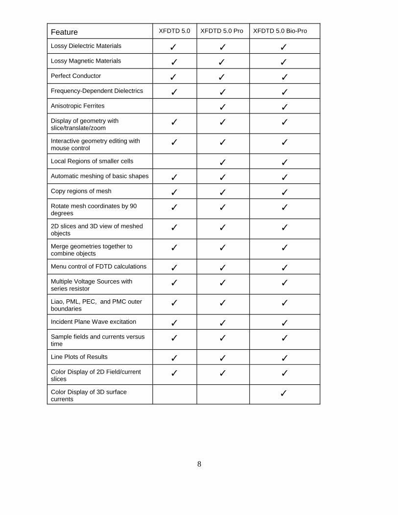
1-3 Summary of XFDTD Features

The features available in each version of XFDTD 5.0 are listed in the table attachedbelow.

8

Feature XFDTD 5.0 XFDTD 5.0 Pro XFDTD 5.0 Bio-Pro

Lossy Dielectric Materials T T T

Lossy Magnetic Materials T T T

Perfect Conductor T T T

Frequency-Dependent Dielectrics T T T

Anisotropic Ferrites T T

Display of geometry withslice/translate/zoom

T T T

Interactive geometry editing withmouse control

T T T

Local Regions of smaller cells T T

Automatic meshing of basic shapes T T T

Copy regions of mesh T T T

Rotate mesh coordinates by 90degrees

T T T

2D slices and 3D view of meshedobjects

T T T

Merge geometries together tocombine objects

T T T

Menu control of FDTD calculations T T T

Multiple Voltage Sources withseries resistor

T T T

Liao, PML, PEC, and PMC outerboundaries

T T T

Incident Plane Wave excitation T T T

Sample fields and currents versustime

T T T

Line Plots of Results T T T

Color Display of 2D Field/currentslices

T T T

Color Display of 3D surfacecurrents

T

9


‘ ‘Movie" sequences of steady-statefields through geometry

T

‘ ‘Movie" sequences of transientfields vs time

T T T

Multiple Voltage/Current Sourceswith Series/Parallel RLC

T T

Input Impedance vs Frequency T T T

Single Frequency Input Impedance T T T

Multi-Port S-Parameters vsFrequency

T T

Multi-Port steady stateS-Parameters

T T

Specific Absorption Ratio (SAR) T

Display Planes of steady-state E, Bfields

T

Display Planes of steady-statecurrent density

T

Adjust SAR level to specified inputpower

T

Calculate 1 and 10 gram SARaverages

T

Location of peak SAR T

SAR ‘ ‘movies" by slicing throughthe mesh

T

TEM cell excitation T

Pre-Meshed human head and body optional

Module for remeshing dielectric withdifferent cell sizes and/or rotation

optional

Module for removing mesh rotationfrom antenna patterns

optional

Circular Polarization Antenna GainPatterns

T T T

Antenna Impedance vs Frequency T T T

Transient Far Zone Transformation T T T

10


Steady State AntennaImpedance/Efficiency

T T T

Antenna Gain vs Frequency T T T

Single Frequency Far ZoneTransformation

T T T

Linear Polarization Antenna Gain vsAngle

T T T

Automatic Meshing of SpiralAntennas

T T T

Thin Wires with different wire radii T T T

Incident Plane Wave T T T

Scattering Cross Sections vsFrequency

T T T

Bi-Static Scattering vs Angle T T T

11

2 Installation and Licensing

The installation and licensing procedure for XFDTD depends on what operating system(Unix or Windows) you have and what version of XFDTD (permanent license orevaluation license) you are installing. There are detailed descriptions of theinstallation procedure provided in two separate documents.

� For evaluation versions of XFDTD, see the document demo_install.pdf.

� For permanent license installations (purchased versions of XFDTD) see thedocument permanent_install.pdf.

12

3 Estimating Computer Resource Requirements

This chapter discusses basic relationships for estimating computer resources requiredfor FDTD calculations. The important aspects of entering the geometry and calculationparameters are discussed. Equations for estimating the amount of memory andcomputer CPU time required for a typical FDTD calculation are provided.

3-1 Defining the Cell Size

The starting point of an FDTD calculation is often deciding the spatial increment, or cellsize, of the structure being simulated. The fundamental constraint on the cell size is that it must be much less than the smallest wavelength for which accurate results aredesired. A commonly applied constraint is "ten cells per wavelength,” meaning that theside of each cell ( x, y, z) should be 1/10 or less at the highest frequency (shortestwavelength) of interest. If the cell size is much larger than this, the Nyquist samplinglimit, = 2 x, is approached too closely for reasonable results to be obtained. Significant aliasing is possible for signal components above the Nyquist limit.

Choosing a cell size of 1/10 is a good starting point, but other factors may require asmaller cell size to be chosen. This topic is covered in more detail later.

Note: FDTD is a volumetric computational method. If some portion of thecomputational space is filled with penetrable material, the wavelength in the materialmust be used to determine the maximum cell size. Geometries containing electricallydense materials require smaller cells than geometries that contain only free space andperfect conductors.

3-1-1 Creating a Geometry with FDTD Cells

Before any FDTD calculation can be done, an accurate approximation of the structureunder test must be entered into XFDTD. As was mentioned above, a resolution ofone-tenth of a wavelength is the minimum required for accurate FDTD results. However, many structures require a higher resolution due to various factors includingcurved surfaces, wire radii, and small details of the structure. An example might be amicrostrip circuit that has a small (<< ) separation distance between the ground planeand the trace. In this case, the driving factor on the cell size will probably be theseparation distance between the ground plane and trace rather than the highestfrequency of interest.

XFDTD uses a “staircase” method of approximating curved surfaces with rectangularcubes. If the structure contains curves, a higher number of cells per wavelength will berequired to reduce the error from the staircased approximation. The exact resolutionrequired will vary, but a good starting point is between 20 and 30 cells per wavelength.

13

XFDTD has a feature known as “subgridding” for approximating small regions of thestructure at a higher resolution. The subgrid can have a resolution of either one-thirdor one-fifth the cell size and is useful in situations where only a small part of thestructure requires the higher resolution for producing an accurate approximation. Subgrids are described in more detail in a later chapter.

3-1-2 Free Space Boundaries

Typically XFDTD makes use of a free space, or absorbing, outer boundary. A numberof cells must separate the structure from this outer boundary to allow better absorptionof the fields. The minimum spacing between the geometry and outer boundary is tencells, although fifteen or more is sometimes required for accurate results. If extremelysmall cells (relative to the wavelength) are used, an outer boundary of approximately1/3 of a wavelength at the lowest frequency of interest should be used, if possible.

3-2 Determining the Total Number of Cells

Once the cell size has been chosen, the total number of cells needed for thecalculation can be found. The number of cells in the x, y, and z directions, often calledNX, NY, and NZ, is determined from the sum of free space boundary cells and thedimensions of the structure in each direction divided by the cell size. The total size ofthe FDTD space in cells is determined by the product of the cells in each dimension. The memory requirements of XFDTD are directly related to the number of cells in thecalculation space. A computer with 128 MB of memory can accommodate calculationsinvolving up to three million cells.

3-3 Estimating the Necessary Computer Resources

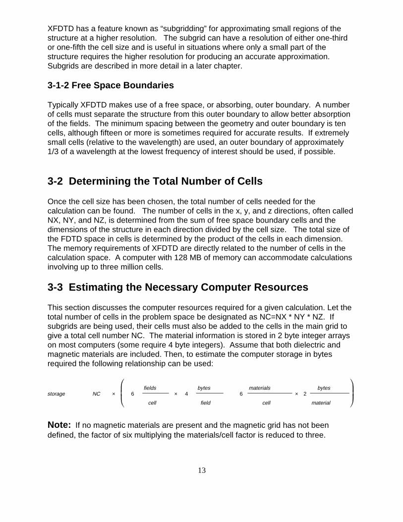
This section discusses the computer resources required for a given calculation. Let thetotal number of cells in the problem space be designated as NC=NX * NY * NZ. Ifsubgrids are being used, their cells must also be added to the cells in the main grid togive a total cell number NC. The material information is stored in 2 byte integer arrayson most computers (some require 4 byte integers). Assume that both dielectric andmagnetic materials are included. Then, to estimate the computer storage in bytesrequired the following relationship can be used:

storage ' NC × 6fields

cell

× 4bytes

field

% 6materials

cell

× 2bytes

material

Note: If no magnetic materials are present and the magnetic grid has not beendefined, the factor of six multiplying the materials/cell factor is reduced to three.

14

This equation neglects the relatively small number of auxiliary variables needed by theprogram. It also neglects the memory needed to store the executable instructions. Since this overhead is nearly independent of the number of cells in the problem space,as the total number of cells increases it will become a smaller fraction of the totalmemory required. However, if the computer memory storage as computed above,exceeds the memory capacity of the computer, then fewer FDTD cells must beused.

This estimate will be low if many far-zone field directions are specified with transientcalculations, especially if the calculation has a large number of time steps. For eachfar-zone direction the program will require six floating-point (4-byte) arrays with a singlearray index slightly larger than the number of time steps specified. This additionalstorage can be easily estimated and added to the above.

For a (100 cell)3 problem space, approximately 30 MBytes of memory would berequired, with the actual amount being somewhat greater due to storage of othervariables and instructions plus memory needed by the operating system. Problems ofthis size can be run on machines ranging from super computers to 32-bit personalcomputers. As available memory is reduced, the maximum number of cells which canbe accommodated is correspondingly decreased. With 16 MBytes of memory, theproblem space size would be estimated from the above relationship as (79 cells)3.

Note: In actual experience 16 MBytes will accommodate approximately (72 cells)3,indicating a memory overhead for instructions and auxiliary variables for this problemsize of about 30% of the memory needed to store the field components. Again, forlarger problem spaces with more cells, this overhead percentage would be reduced.

3-3-1 Far-Zone Radiation angles at a single frequency

The steady-state calculation option and its associated steady-state far-zonetransformation allow for unlimited far-zone calculations in post-processing. With thisoption the complex tangential fields on a closed surface surrounding the radiatingstructure are determined at the end of the FDTD calculation. These tangential fieldsare then used by XFDTD to obtain far-zone radiation gain (or bistatic scattering) in anydirection during post-processing. This eliminates the time and memory required formany transient far-zone radiation directions. However, this method provides resultsonly at the frequency of the input.

3-3-2 Execution Time Estimation

Another way to estimate the computational cost is by calculating the number of floating-point operations required. This method involves estimating the total number of timesteps to be calculated. As a preliminary estimate, the time required for energy travelingat the speed of light to traverse the geometry five times may be used. With a transientinput, convergence of the calculation can be determined by observing the feed-point

15

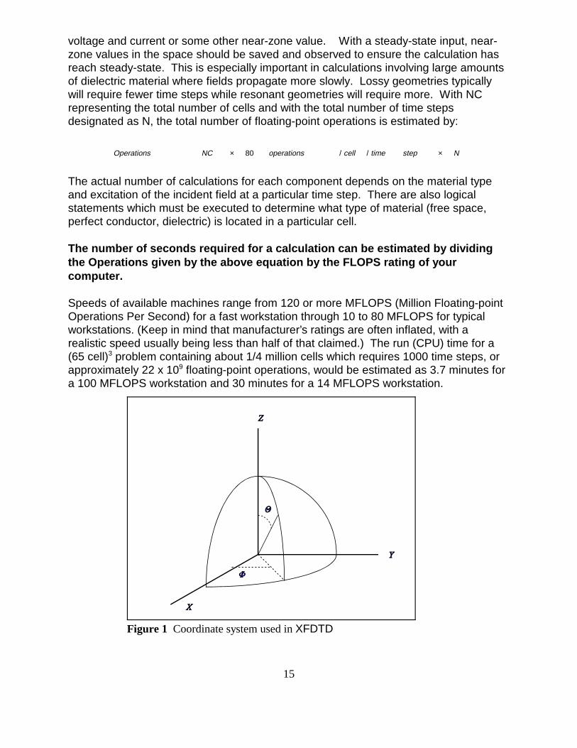
Figure 1 Coordinate system used in XFDTD

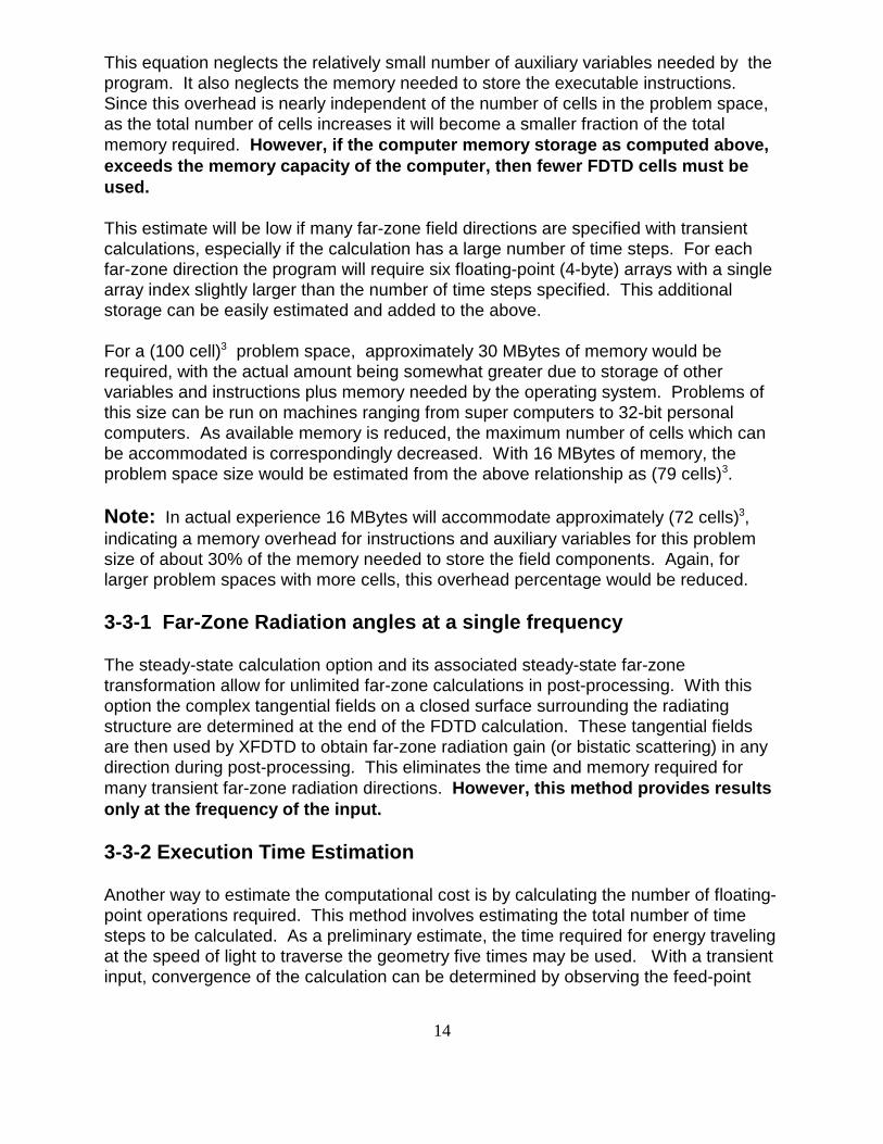
voltage and current or some other near-zone value. With a steady-state input, near-zone values in the space should be saved and observed to ensure the calculation hasreach steady-state. This is especially important in calculations involving large amountsof dielectric material where fields propagate more slowly. Lossy geometries typicallywill require fewer time steps while resonant geometries will require more. With NCrepresenting the total number of cells and with the total number of time stepsdesignated as N, the total number of floating-point operations is estimated by:

Operations ' NC × 80 operations / cell / time step × N

The actual number of calculations for each component depends on the material typeand excitation of the incident field at a particular time step. There are also logicalstatements which must be executed to determine what type of material (free space,perfect conductor, dielectric) is located in a particular cell.

The number of seconds required for a calculation can be estimated by dividingthe Operations given by the above equation by the FLOPS rating of yourcomputer.

Speeds of available machines range from 120 or more MFLOPS (Million Floating-pointOperations Per Second) for a fast workstation through 10 to 80 MFLOPS for typicalworkstations. (Keep in mind that manufacturer’s ratings are often inflated, with arealistic speed usually being less than half of that claimed.) The run (CPU) time for a(65 cell)3 problem containing about 1/4 million cells which requires 1000 time steps, orapproximately 22 x 109 floating-point operations, would be estimated as 3.7 minutes fora 100 MFLOPS workstation and 30 minutes for a 14 MFLOPS workstation.

16

3-4 Coordinate System

The coordinate system used in XFDTD is shown in Figure 1. Geometries aredescribed in Cartesian X, Y, Z coordinates. Distances may be measured in spatialincrements x, y, z, with integer indices I, J, K locating points in the FDTD space asx=I x. etc. Far-zone directions are measured using spherical coordinates and . For far-zone field amplitude calculations the far-zone distance is normalized to 1 meter.

17

4 XFDTD Graphical User Interface

XFDTD is a graphical user interface to an FDTD calculation program. With XFDTD electromagnetic simulations can be performed quickly and easily. From within XFDTDthe object under consideration can be entered with the editing tools, the calculationparameters for the input and output selected using informative menus, and the results displayed in a variety of formats. This chapter of the manual contains an overview ofthe entire interface. More detailed descriptions of the menu options are found in otherchapters.

NOTE: The Windows NT/95/98 version of XFDTD and the UNIX version of XFDTDhave slightly different formats. Whenever important differences exist between theversions, mention will be made. The term “windows version” will refer to the WindowsNT/95/98 version of XFDTD while “UNIX version” will refer to XFDTD for any UNIXplatform.

4-1 Starting XFDTD

4-1-1 Starting XFDTD in Windows NT/95/98

In Windows NT or Windows 95/98, go to the Start Menu, select Programs, thenREMCOM, and finally XFDTD 5.0.

4-1-2 Starting XFDTD in UNIX

To start XFDTD from a Unix installation, enter the command "xfdtd504”. Remember,the XFDTD program files xfdtd504, calcfdtd504, xpostp50, and xpostpss50 must bein the PATH or in the current directory and all files must have execute permission. It isbest to make separate directories for each calculation. Consequently, it is best to startXFDTD from the desired output directory.

4-2 The XFDTD User Interface

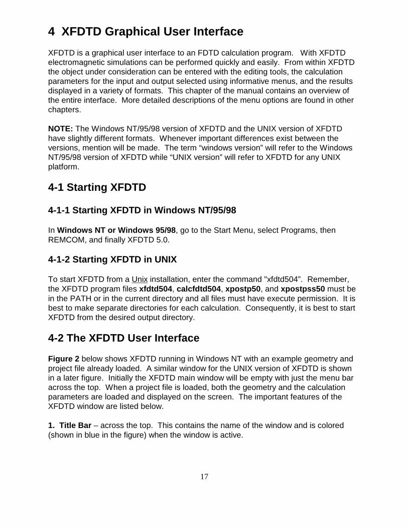
Figure 2 below shows XFDTD running in Windows NT with an example geometry andproject file already loaded. A similar window for the UNIX version of XFDTD is shownin a later figure. Initially the XFDTD main window will be empty with just the menu bar across the top. When a project file is loaded, both the geometry and the calculationparameters are loaded and displayed on the screen. The important features of theXFDTD window are listed below.

1. Title Bar – across the top. This contains the name of the window and is colored(shown in blue in the figure) when the window is active.

18

Figure 2: XFDTD window as seen on a Windows NT/95/98 computer.

Figure 3: The Tool Bar in XFDTD 5.0

2. Menu Bar – pulldown menus for File, Edit, View, Window when viewing thegeometry file. When viewing the Run Parameters window the “Results” entry is alsoadded. The menu bar on the UNIX version of XFDTD will always display all the optionsas there are not separate windows for Geometry and Run Parameters.

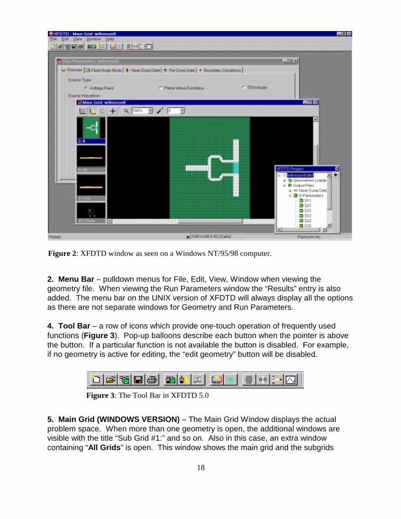
4. Tool Bar – a row of icons which provide one-touch operation of frequently usedfunctions (Figure 3). Pop-up balloons describe each button when the pointer is abovethe button. If a particular function is not available the button is disabled. For example,if no geometry is active for editing, the “edit geometry” button will be disabled.

5. Main Grid (WINDOWS VERSION) – The Main Grid Window displays the actualproblem space. When more than one geometry is open, the additional windows arevisible with the title “Sub Grid #1:” and so on. Also in this case, an extra windowcontaining “All Grids” is open. This window shows the main grid and the subgrids

19

together. Each of these windows allows selection of the viewing plane and providesspecific tools by which to manipulate the geometry. Note that editing is disabled in the“All Grids” window. When any one of these windows is active, features such as thebackground grid, the electric or magnetic components, and normal elements can beturned on and off. Also, the zoom and slice features are functional. Select thecoordinate plane in which to view the geometry by clicking on one of the three panesalong the left side of the window. For each window, except the “All Grids” window, the3D View is available displaying the entire problem space in three dimensions.

Panning in XY, YZ, and XZ planes in Windows

If the Geometry window is active, the current coordinate system of the geometry is shown in blue along the left-hand side of the window. When the mouse pointer ismoved over these panes, a hand icon appears. By holding down the left mouse buttonwhile the cursor is over a coordinate system window, the hand “grabs” the window andallows panning of the viewed portion of the geometry to center features of interest. Furthermore, each coordinate plane zooms independently of the others.

Other controls of the geometry window

The zoom button increases or decreases the scale of the geometrydrawn in the window. By pressing the magnifying glass at the left of thezoom figure, the mouse buttons may be used to perform the zooming.

The left mouse button zooms in and the right mouse button zooms out. A region maybe defined with the mouse in (when the icon is a magnifying glass) and this view willzoom in on this region. To turn off zooming, click the magnifying glass button again. Double-clicking on the magnifying glass sets the zoom back to 100%. The zoom canalso be changed by simply pressing the up and down arrows next to the text displayingthe zoom scale or by typing a zoom amount into the text area.

The slice currently in view is changed by pressing the up or down arrowsor by simply typing the desired slice into the text area.

This button toggles the “normal” components view. Since the window is two-dimensional, components normal to the view are be displayed as dots.

This button toggles the drawing of the grid representing entire geometry space. Turning on this grid is especially helpful when editing the geometry.

This button toggles the drawing of the electric components of the geometry. When viewing fields or editing the magnetic grid, it is sometimes useful to turn offthe geometry.

20

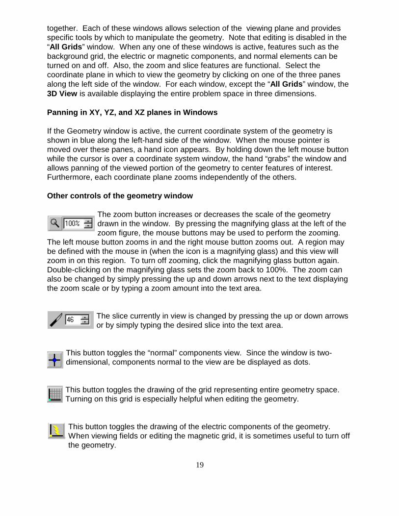
Figure 4: The XFDTD 5.0 interface on a UNIX computer.

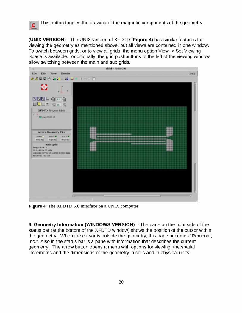
This button toggles the drawing of the magnetic components of the geometry.

(UNIX VERSION) - The UNIX version of XFDTD (Figure 4) has similar features forviewing the geometry as mentioned above, but all views are contained in one window. To switch between grids, or to view all grids, the menu option View -> Set ViewingSpace is available. Additionally, the grid pushbuttons to the left of the viewing windowallow switching between the main and sub grids.

6. Geometry Information (WINDOWS VERSION) – The pane on the right side of thestatus bar (at the bottom of the XFDTD window) shows the position of the cursor withinthe geometry. When the cursor is outside the geometry, this pane becomes “Remcom,Inc.”. Also in the status bar is a pane with information that describes the currentgeometry. The arrow button opens a menu with options for viewing the spatialincrements and the dimensions of the geometry in cells and in physical units.

21

Figure 5: The XFDTD Run Parameters window available in the Windows Version.

(UNIX VERSION) - The display for the location of the pointer is in the upper left cornerof the geometry window. The spatial increments, number of cells, and other informationis displayed in the information area at the left of the geometry display.

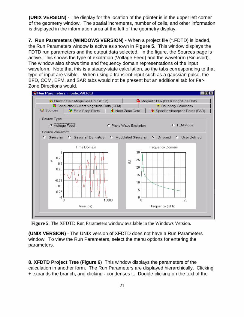
7. Run Parameters (WINDOWS VERSION) - When a project file (*.FDTD) is loaded,the Run Parameters window is active as shown in Figure 5. This window displays theFDTD run parameters and the output data selected. In the figure, the Sources page isactive. This shows the type of excitation (Voltage Feed) and the waveform (Sinusoid).The window also shows time and frequency domain representations of the inputwaveform. Note that this is a steady-state calculation, so the tabs corresponding to thattype of input are visible. When using a transient input such as a gaussian pulse, theBFD, CCM, EFM, and SAR tabs would not be present but an additional tab for Far-Zone Directions would.

(UNIX VERSION) - The UNIX version of XFDTD does not have a Run Parameterswindow. To view the Run Parameters, select the menu options for entering theparameters.

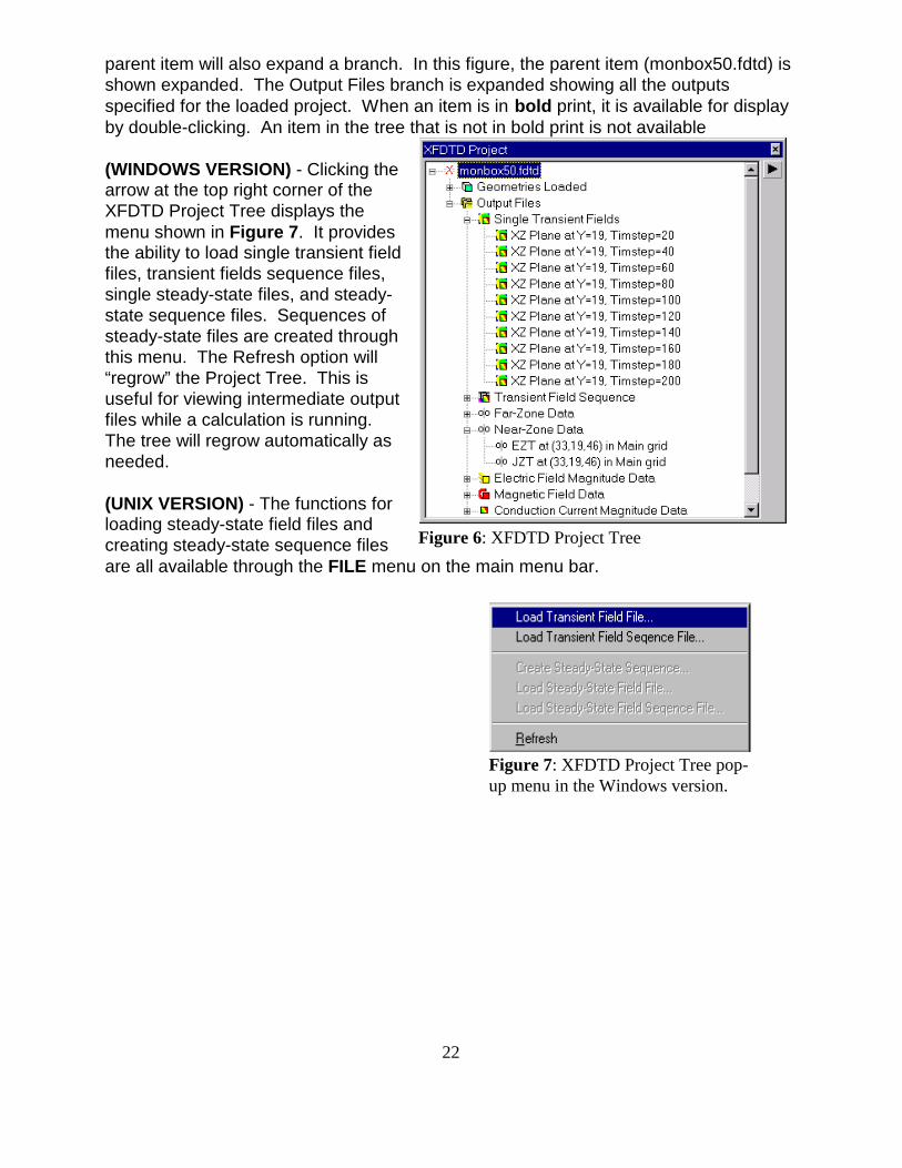
8. XFDTD Project Tree (Figure 6) This window displays the parameters of thecalculation in another form. The Run Parameters are displayed hierarchically. Clicking+ expands the branch, and clicking - condenses it. Double-clicking on the text of the

22

Figure 6: XFDTD Project Tree

Figure 7: XFDTD Project Tree pop-up menu in the Windows version.

parent item will also expand a branch. In this figure, the parent item (monbox50.fdtd) isshown expanded. The Output Files branch is expanded showing all the outputsspecified for the loaded project. When an item is in bold print, it is available for displayby double-clicking. An item in the tree that is not in bold print is not available

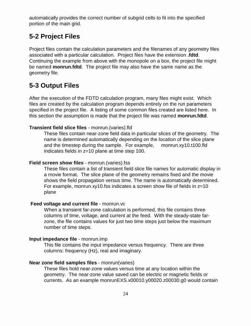
(WINDOWS VERSION) - Clicking thearrow at the top right corner of theXFDTD Project Tree displays themenu shown in Figure 7. It providesthe ability to load single transient fieldfiles, transient fields sequence files,single steady-state files, and steady-state sequence files. Sequences ofsteady-state files are created throughthis menu. The Refresh option will“regrow” the Project Tree. This isuseful for viewing intermediate outputfiles while a calculation is running. The tree will regrow automatically asneeded.

(UNIX VERSION) - The functions forloading steady-state field files andcreating steady-state sequence filesare all available through the FILE menu on the main menu bar.

23

5 File Types

XFDTD creates many different files for storing the geometry, calculation parameters,and output. This chapter focuses on the types of files written by XFDTD. All outputdata from the calculation are viewed through the XFDTD interface and knowledge ofthe actual filenames is not required. For users who wish to use the output data froman XFDTD calculation in another program, a detailed listing of the output file formats isgiven in a later chapter. Here a brief listing of the files created is given here as aguide.

Note: In this chapter the base file names of monbox and monrun will be used asexamples. In actual use of XFDTD, these names are given within the program.

5-1 Geometry Files

Geometry files contain the data describing the location and content of the FDTD cells. These files always have the extension .id. For example, the geometry of a monopoleon a rectangular box might be saved as the file monbox.id.

A geometry (often referred to as “.id” file) may be either a main grid or a subgrid. Thusa geometry file may be used alone for calculations, or it may be used as a subgrid witha different geometry file serving as the main grid. This removes the necessity forhaving two different types of geometry files, while also allowing the use of the samemesh in a different calculation. For example, an antenna can be meshed andcalculations made on it as a main grid. Then this same antenna geometry file can beused as a subgrid, in conjunction with a main grid mesh using larger cells of a vehicleon which the antenna is located. When used as a subgrid, the cells for the geometrymust be smaller than those of the file used as the main grid mesh. Alternatively the twogrids can be merged into one mesh with the same cell size.

Ratios between Main Grids and Subgrids

There is a constraint on subgrid meshes that the cell ratios between the main grid andsubgrid must be fixed at odd integer ratios. That is, the subgrid cells must be one-thirdor one-fifth the size (in each edge dimension) of the main grid cells. Also the numberof cells in each dimension of the subgrid geometry must align properly with the maingrid. For proper alignment, the subgrid dimension NX, NY, and NZ must be evenlydivisible by either three or five, depending on the ratio of the subgrid. If a geometryfile does not fit properly, a new mesh can be created that has the correct dimensionsand the geometry can be merged into it. The Merge feature is covered in a latersection of the manual.

If a main grid is first created or read into XFDTD and then a subgrid is created, thesubgrid dimensions are entered as a number of main grid cells, and XFDTD

24

automatically provides the correct number of subgrid cells to fit into the specifiedportion of the main grid.

5-2 Project Files

Project files contain the calculation parameters and the filenames of any geometry filesassociated with a particular calculation. Project files have the extension .fdtd. Continuing the example from above with the monopole on a box, the project file mightbe named monrun.fdtd. The project file may also have the same name as thegeometry file.

5-3 Output Files

After the execution of the FDTD calculation program, many files might exist. Whichfiles are created by the calculation program depends entirely on the run parametersspecified in the project file. A listing of some common files created are listed here. Inthis section the assumption is made that the project file was named monrun.fdtd. Transient field slice files - monrun.(varies).fld

These files contain near-zone field data in particular slices of the geometry. Thename is determined automatically depending on the location of the slice planeand the timestep during the sample. For example, monrun.xy10.t100.fldindicates fields in z=10 plane at time step 100.

Field screen show files - monrun.(varies).fssThese files contain a list of transient field slice file names for automatic display ina movie format. The slice plane of the geometry remains fixed and the movieshows the field propagation versus time. The name is automatically determined. For example, monrun.xy10.fss indicates a screen show file of fields in z=10plane

Feed voltage and current file - monrun.vcWhen a transient far-zone calculation is performed, this file contains threecolumns of time, voltage, and current at the feed. With the steady-state far-zone, the file contains values for just two time steps just below the maximumnumber of time steps.

Input impedance file - monrun.impThis file contains the input impedance versus frequency. There are threecolumns: frequency (Hz), real and imaginary.

Near zone field samples files - monrun(varies)These files hold near-zone values versus time at any location within thegeometry. The near-zone value saved can be electric or magnetic fields orcurrents. As an example monrunEXS.x00010.y00020.z00030.g0 would contain

25

the x-directed electric field component at cell location x,y,z (i,j,k) 10,20,30 issaved.

Steady-State Field Quantities - monrun.(varies).sar, .cef, .bfd, .ccmThese files contain steady-state field magnitudes in a particular slice of thegeometry. The steady-state values that can be saved include SAR (specificabsorption rate) files, electric field magnitudes, magnetic flux densitymagnitudes, or conduction currents. These files can be made into movies thatshow the fields versus position in the geometry.

Diagnostics file - fdtd.diagThis file provides some basic information about the FDTD calculationparameters including problem space size, cell size, time step size, and numberof time steps calculated. Information on excitation, either pulse or sinusoidal, isalso provided.

Progress file - tsfdtdThis file contains information regarding the progress of an FDTD calculation. Typically it contains three numbers: current time step, total number of time steps,percent completion.

There are various other files created by the FDTD calculation program that are used forpostprocessing data. For example files ending in .fza, .fzb , and .fzin are used only bythe postprocessors xpostpss50 and xpostp50. Additionally there are files created bythe postprocessors such as antenna gain patterns or averaged SAR values.

26

Figure 8: File Menu

Figure 9: Create New Grid

6 The File Menu

The menus in the Windows version of XFDTD are standardized to match commonWindows NT and Windows 95/98 applications. This chapter will discuss the first menuoption, the File menu. As the UNIX version of XFDTD follows a different format, it iscovered in a separate section of the chapter that follows the Windows section.

6-1 The File Menu in Windows NT/95/98

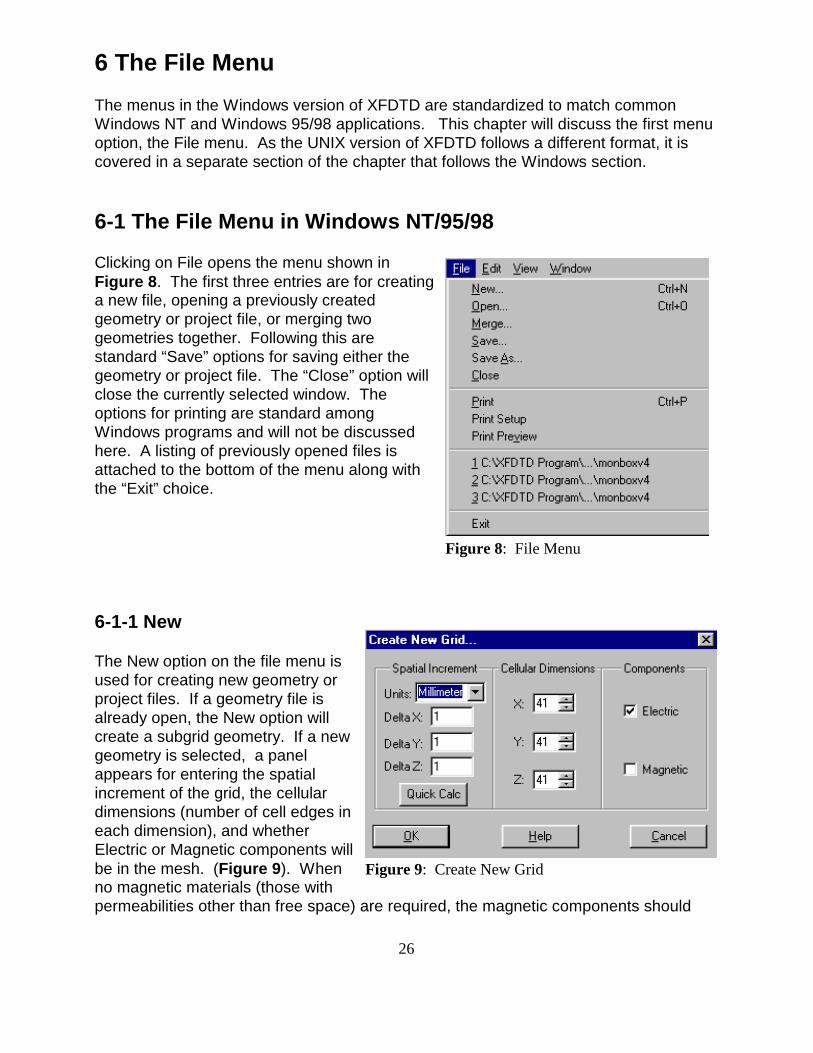
Clicking on File opens the menu shown inFigure 8. The first three entries are for creatinga new file, opening a previously createdgeometry or project file, or merging twogeometries together. Following this arestandard “Save” options for saving either thegeometry or project file. The “Close” option willclose the currently selected window. Theoptions for printing are standard amongWindows programs and will not be discussedhere. A listing of previously opened files isattached to the bottom of the menu along withthe “Exit” choice.

6-1-1 New

The New option on the file menu isused for creating new geometry orproject files. If a geometry file isalready open, the New option willcreate a subgrid geometry. If a newgeometry is selected, a panelappears for entering the spatialincrement of the grid, the cellulardimensions (number of cell edges ineach dimension), and whetherElectric or Magnetic components willbe in the mesh. (Figure 9). Whenno magnetic materials (those withpermeabilities other than free space) are required, the magnetic components should

27

not be selected. The Quick Calc option displays the frequency and wavelength thatcorrespond to 10 cells per wavelength at the current spatial increment

If no geometry files are already open in XFDTD, selecting New will create a new maingrid. When specifying the spatial increments (cell size) in the x, y, and z directions, thecells should not deviate greatly from cubical. A reasonable rule is to keep all cellincrements (cell edges) to within a factor of two in size. The cell size is determined byboth the geometry features and by the highest frequency. The cells should be smallenough to describe the important geometry features, and no larger than approximatelyone-tenth of the shortest wavelength of interest. If the geometry includes dielectricand/or magnetic material, the wavelength inside these materials must be consideredsince it will be shorter than in the free space region of the FDTD space.

If a geometry already exists when the New geometry is selected, the “ConfigureSubgrid” menu opens. This menu prompts for the subgrid offset within the main grid and the ratio of the subgrid cells. The offset refers to the displacement of the origin ofthe subgrid relative to the origin of the main grid. This positions the subgrid within themain grid. The ratio refers to the cell size of the subgrid in relation to the main gridcells. Ratios of either one-third or one-fifth may be selected.

Note: the subgrid mesh appears to overlap slightly the main grid mesh. This is normaland is caused by the mesh interpolation of the magnetic fields rather than electricfields. For a cell size ratio of one-third, each of the grid dimensions NX, NY, NZ for thesubgrid must be evenly divisible by three (ie NX/3 is an integer). For proper fieldinterpolation each subgrid dimension should be at least 4 main grid cells. Thus for aone-third cell subgrid, the minimum grid dimensions are 12 x 12 x 12 subgrid cells. Inaddition, if two subgrids are specified, both must have the same cell size.

After setting the offset and ratio of the new subgrid, the “Create New Geometry” panel(Figure 9) will open and prompt for the same information as a main grid. However,when a subgrid is created, the spatial increment has already been selectedautomatically and should not be modified. The “Number of Cells” requested is in maingrid cells, not subgrid cells. So, entering an NX value of 4 with a 3:1 subgrid will createa new subgrid with an NX of 12.

Subgrids may be specified to contain magnetic materials but for all calculations thesubgrid space is assumed to have free space permeability and no magnetic materialswill be visible in the subgrid. If the subgrid is also used as a main grid in a separateproject, then the magnetic grid may be edited and used.

28

6-1-2 Open

This option opens geometry or project files that have already been created. To open afile, either double click on the file or select it with the mouse and the select Open.The project files contain the XFDTD calculation parameters and the geometry file name(including subgrids), so opening a project file will also open the geometry.

6-1-3 Merge

This feature merges two geometry files. It is especially useful for modifying an existinggeometry by placing it in a new mesh that may be larger or smaller than the original. The Merge function prompts for a vector offset which allows for repositioning of onegeometry within another. Geometries can be merged into the main grid or one of thesubgrids.

One application of using the Merge function might be when one geometry contains ahuman head and another contains a portable telephone. The two geometries can bemerged together to place the telephone near the head. The resulting mesh can besaved as a new geometry file. This procedure can be repeated and with the telephonein a different position. Another use of the Merge function is creating subgrids from existing main grid geometryfiles. If the grid dimensions of a geometry file are not correct for use as a subgrid, thegeometry can be merged into a mesh of the proper dimensions and saved as a new file.

6-1-4 Save

This option saves either the geometry or calculation parameters, depending on whichwindow is currently active. The main grid geometry and any existing subgrids aresaved separately. If the file has not been saved before, a filename must be entered. Otherwise the file will be saved with the same name. XFDTD automatically suppliesthe suffix to the file name (either .id for a geometry file or .fdtd for a project file). Thefilename for geometry and project files can be the same, but it does not have to be.

Before writing a project file the corresponding geometry file for the main grid and forany subgrids must be saved. Also, some calculation parameters for both inputs andoutputs must be set before a project file can be saved.

6-1-5 Save As

This option functions identically to the Save function above except it prompts for afilename. “Save As” will not automatically save a file under the same name.

29

Figure 10: The File menu in the UNIX version of XFDTD 5.0

6-1-6 Close

The Close option closes the currently active window which may be a geometry orproject file. Typically before loading a new geometry or project, any existing file shouldbe closed. Before closing a file, XFDTD determines if the file has been modified andasks if the file should be saved before closing.

6-1-7 Exit

Select this option to exit XFDTD. XFDTD will ask if any unsaved files should be saved

6-2 The File Menu in UNIX XFDTD

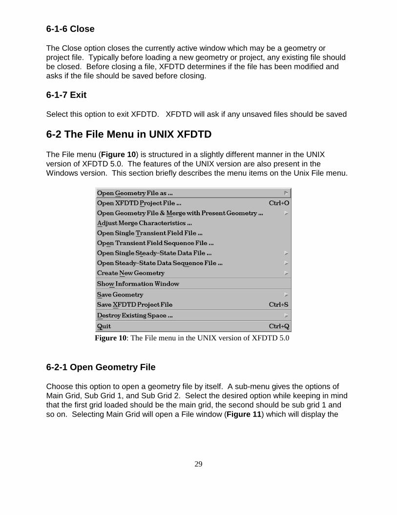
The File menu (Figure 10) is structured in a slightly different manner in the UNIXversion of XFDTD 5.0. The features of the UNIX version are also present in theWindows version. This section briefly describes the menu items on the Unix File menu.

6-2-1 Open Geometry File

Choose this option to open a geometry file by itself. A sub-menu gives the options ofMain Grid, Sub Grid 1, and Sub Grid 2. Select the desired option while keeping in mindthat the first grid loaded should be the main grid, the second should be sub grid 1 andso on. Selecting Main Grid will open a File window (Figure 11) which will display the

30

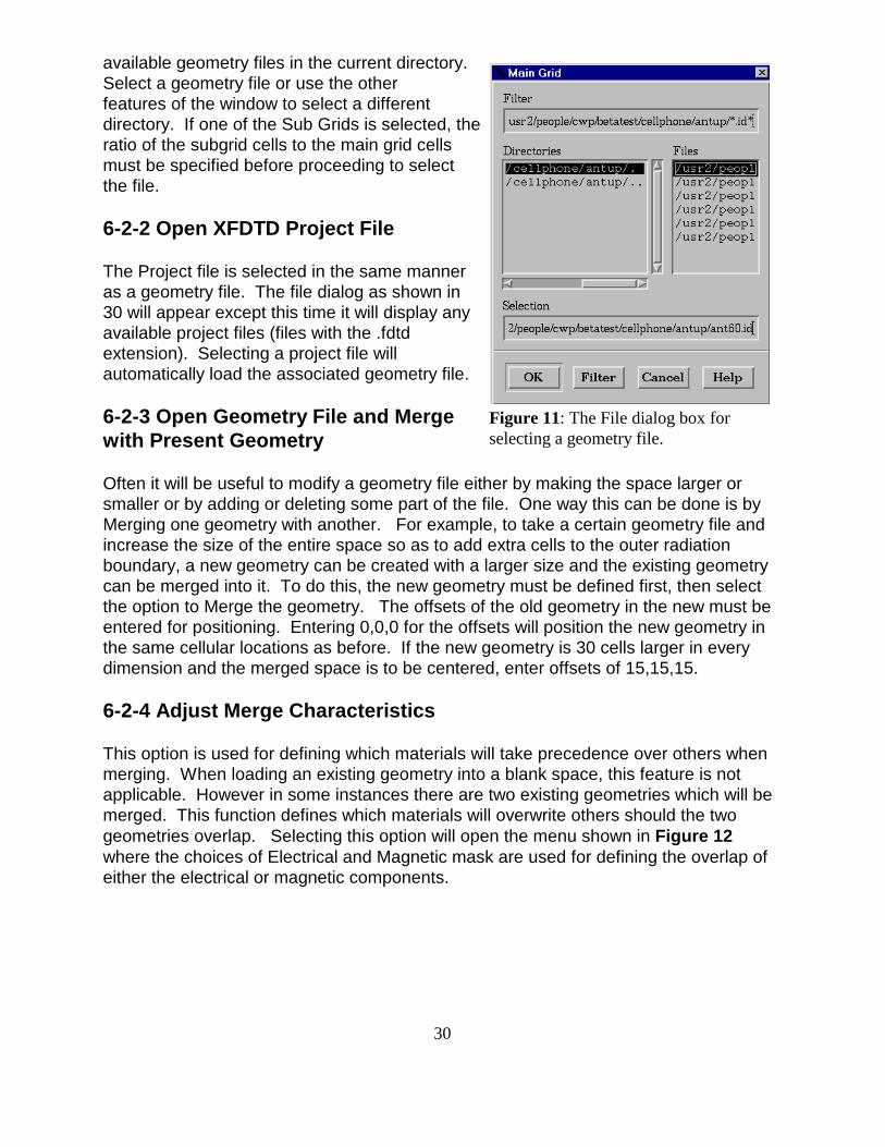
Figure 11: The File dialog box forselecting a geometry file.

available geometry files in the current directory. Select a geometry file or use the otherfeatures of the window to select a differentdirectory. If one of the Sub Grids is selected, theratio of the subgrid cells to the main grid cellsmust be specified before proceeding to selectthe file.

6-2-2 Open XFDTD Project File

The Project file is selected in the same manneras a geometry file. The file dialog as shown in30 will appear except this time it will display anyavailable project files (files with the .fdtdextension). Selecting a project file willautomatically load the associated geometry file.

6-2-3 Open Geometry File and Mergewith Present Geometry

Often it will be useful to modify a geometry file either by making the space larger orsmaller or by adding or deleting some part of the file. One way this can be done is byMerging one geometry with another. For example, to take a certain geometry file andincrease the size of the entire space so as to add extra cells to the outer radiationboundary, a new geometry can be created with a larger size and the existing geometrycan be merged into it. To do this, the new geometry must be defined first, then selectthe option to Merge the geometry. The offsets of the old geometry in the new must beentered for positioning. Entering 0,0,0 for the offsets will position the new geometry inthe same cellular locations as before. If the new geometry is 30 cells larger in everydimension and the merged space is to be centered, enter offsets of 15,15,15.

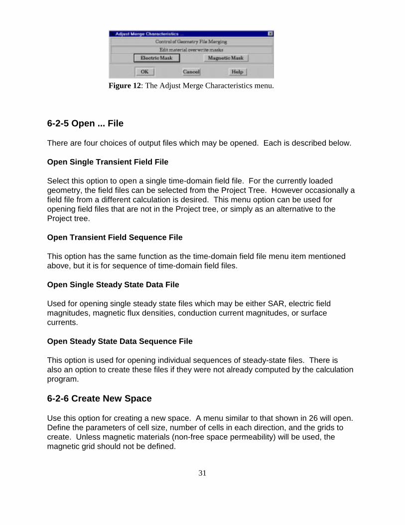
6-2-4 Adjust Merge Characteristics

This option is used for defining which materials will take precedence over others whenmerging. When loading an existing geometry into a blank space, this feature is notapplicable. However in some instances there are two existing geometries which will bemerged. This function defines which materials will overwrite others should the twogeometries overlap. Selecting this option will open the menu shown in Figure 12where the choices of Electrical and Magnetic mask are used for defining the overlap ofeither the electrical or magnetic components.

31

Figure 12: The Adjust Merge Characteristics menu.

6-2-5 Open ... File

There are four choices of output files which may be opened. Each is described below.

Open Single Transient Field File

Select this option to open a single time-domain field file. For the currently loadedgeometry, the field files can be selected from the Project Tree. However occasionally afield file from a different calculation is desired. This menu option can be used foropening field files that are not in the Project tree, or simply as an alternative to theProject tree.

Open Transient Field Sequence File

This option has the same function as the time-domain field file menu item mentionedabove, but it is for sequence of time-domain field files.

Open Single Steady State Data File

Used for opening single steady state files which may be either SAR, electric fieldmagnitudes, magnetic flux densities, conduction current magnitudes, or surfacecurrents.

Open Steady State Data Sequence File

This option is used for opening individual sequences of steady-state files. There isalso an option to create these files if they were not already computed by the calculationprogram.

6-2-6 Create New Space

Use this option for creating a new space. A menu similar to that shown in 26 will open. Define the parameters of cell size, number of cells in each direction, and the grids tocreate. Unless magnetic materials (non-free space permeability) will be used, themagnetic grid should not be defined.

32

6-2-7 Show Information Window

This option opens a separate window with information about the loaded geometry.

6-2-8 Save Geometry

Select this option to save a geometry file. Select whether the file should be saved aseither a main grid or a subgrid. A File box will open allowing the directory and filenameof the geometry to be entered.

6-2-9 Save XFDTD Project File

This saves the Project file currently loaded.

6-2-10 Destroy Existing Space

If a geometry is loaded but no longer desired, it can be removed with this option. Thisis useful for removing a subgrid from a project.

6-2-11 Quit

Select this option to exit the XFDTD program.

33

Figure 13: The Edit menu of theGeometry window in the Windowsversion of XFDTD 5.0.

7 Edit Menu - Geometry

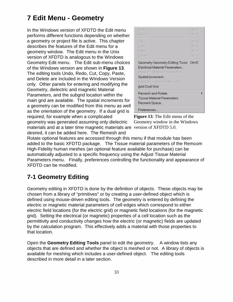
In the Windows version of XFDTD the Edit menuperforms different functions depending on whethera geometry or project file is active. This chapterdescribes the features of the Edit menu for ageometry window. The Edit menu in the Unixversion of XFDTD is analogous to the WindowsGeometry Edit menu. The Edit sub-menu choicesof the Windows version are shown in Figure 13. The editing tools Undo, Redo, Cut, Copy, Paste,and Delete are included in the Windows Versiononly. Other panels for entering and modifying theGeometry, dielectric and magnetic MaterialParameters, and the subgrid location within themain grid are available. The spatial increments fora geometry can be modified from this menu as wellas the orientation of the geometry. If a dual grid isrequired, for example when a complicatedgeometry was generated assuming only dielectricmaterials and at a later time magnetic materials aredesired, it can be added here. The Remesh andRotate optional features are accessed through this menu if that module has beenadded to the basic XFDTD package. The Tissue material parameters of the RemcomHigh-Fidelity human meshes (an optional feature available for purchase) can beautomatically adjusted to a specific frequency using the Adjust Tissue MaterialParameters menu. Finally, preferences controlling the functionality and appearance ofXFDTD can be modified.

7-1 Geometry Editing

Geometry editing in XFDTD is done by the definition of objects. These objects may bechosen from a library of “primitives” or by creating a user-defined object which isdefined using mouse-driven editing tools. The geometry is entered by defining theelectric or magnetic material parameters of cell edges which correspond to eitherelectric field locations (for the electric grid) or magnetic field locations (for the magneticgrid). Setting the electrical (or magnetic) properties of a cell location such as thepermittivity and conductivity changes how the electric (or magnetic) fields are updatedby the calculation program. This effectively adds a material with those properties tothat location. Open the Geometry Editing Tools panel to edit the geometry. A window lists anyobjects that are defined and whether the object is meshed or not. A library of objects isavailable for meshing which includes a user-defined object. The editing toolsdescribed in more detail in a later section.

34

Figure 14: EditElectric Materialspanel

A material palette is included in Windows for adding new dielectric or magneticmaterials and defining their properties. The Electrical and Magnetic MaterialParameters menus provide the Material Palette function in the UNIX version.

7-2 The Material Palette - Windows Version Only

In Windows when Geometry..., Electric Material Parameters..., orEdit Magnetic Materials is selected, the corresponding MaterialPalette appears. Figure 14 shows the Electrical MaterialsPalette. Each color on the palette represents a different materialtype. Black (number 0) and White (number 1) always correspondto free space and Perfect Electric Conductor (PEC) respectivelyand cannot be changed. To add a new user-defined material type,click Add... . Either the next available material may be selected ora particular color. Each color represents a particular materialthough and may only be used once. To aid in identifying differentmaterials, a material description may be entered in the areaprovided. XFDTD will store this name with the other materialparameters to allow easy identification of different materials. Ifediting electrical materials, there is also the option to Add Thin Wire. Thin wires maybe used when the geometry requires a wire with a very thin radius which is much lessthan the cell size. It should be noted that a wire constructed of a single edge of PEC has an effective radius of approximately ¼ of a cell. Thin wires always appear withcross-hatched color.

7-3 Specifying Electrical Materials

Often materials other than free space and perfect electric conductor are needed for aparticular geometry. To create a new material in Windows, select Add... from theMaterial Palette. You can choose whether you want the next available color orwhether you want to select a specific color. Either choice brings up the Edit ElectricMaterial window (Figure 15). In the Unix version the equivalent operation is to openthe Electrical Materials Parameter Window from the Edit->Geometry menu.

Clicking this button on the tool bar will display the Electric Materials Palette(Windows) and display the electric components of the grid.

The Edit Electric Material window (for Windows) or the Electrical Material Parameterswindow (for Unix) is used to edit the values of constitutive parameters for dielectricmaterials, including frequency-dependent dielectrics. XFDTD has three options fordielectric material models. For a normal dielectric, one in which the electricalproperties do not vary significantly with frequency, the conductivity in Siemens/meter

35

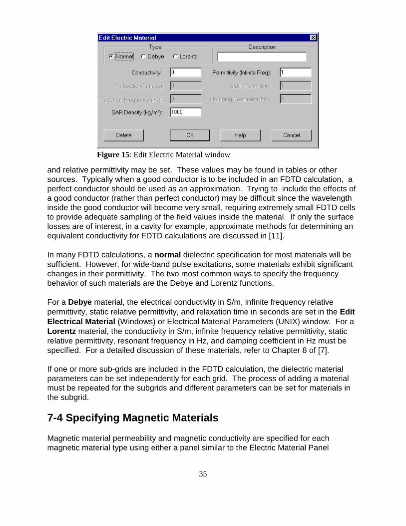
Figure 15: Edit Electric Material window

and relative permittivity may be set. These values may be found in tables or othersources. Typically when a good conductor is to be included in an FDTD calculation, aperfect conductor should be used as an approximation. Trying to include the effects ofa good conductor (rather than perfect conductor) may be difficult since the wavelengthinside the good conductor will become very small, requiring extremely small FDTD cellsto provide adequate sampling of the field values inside the material. If only the surfacelosses are of interest, in a cavity for example, approximate methods for determining anequivalent conductivity for FDTD calculations are discussed in [11].

In many FDTD calculations, a normal dielectric specification for most materials will besufficient. However, for wide-band pulse excitations, some materials exhibit significantchanges in their permittivity. The two most common ways to specify the frequencybehavior of such materials are the Debye and Lorentz functions.

For a Debye material, the electrical conductivity in S/m, infinite frequency relativepermittivity, static relative permittivity, and relaxation time in seconds are set in the EditElectrical Material (Windows) or Electrical Material Parameters (UNIX) window. For aLorentz material, the conductivity in S/m, infinite frequency relative permittivity, staticrelative permittivity, resonant frequency in Hz, and damping coefficient in Hz must bespecified. For a detailed discussion of these materials, refer to Chapter 8 of [7].

If one or more sub-grids are included in the FDTD calculation, the dielectric materialparameters can be set independently for each grid. The process of adding a materialmust be repeated for the subgrids and different parameters can be set for materials inthe subgrid.

7-4 Specifying Magnetic Materials

Magnetic material permeability and magnetic conductivity are specified for eachmagnetic material type using either a panel similar to the Electric Material Panel

36

Figure 16: Defining an anisotropic magneticmaterial in XFDTD 5.0.

(Windows) or a menu analogous to the Electrical Material Parameters menu (UNIX). These choices are only available if the magnetic grid was created with the geometry. Ifthe magnetic is grid is desired but does not exist, it can be added through the “AddDual Grid” function (discussed later).

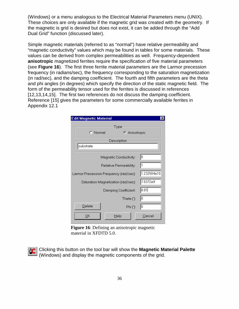
Simple magnetic materials (referred to as “normal”) have relative permeability and“magnetic conductivity” values which may be found in tables for some materials. Thesevalues can be derived from complex permeabilities as well. Frequency-dependentanisotropic magnetized ferrites require the specification of five material parameters(see Figure 16). The first three ferrite material parameters are the Larmor precessionfrequency (in radians/sec), the frequency corresponding to the saturation magnetization(in rad/sec), and the damping coefficient. The fourth and fifth parameters are the thetaand phi angles (in degrees) which specify the direction of the static magnetic field. Theform of the permeability tensor used for the ferrites is discussed in references[12,13,14,15]. The first two references do not discuss the damping coefficient.Reference [15] gives the parameters for some commercially available ferrites inAppendix 12.1

Clicking this button on the tool bar will show the Magnetic Material Palette(Windows) and display the magnetic components of the grid.

37

Figure 17: Edit Thin Wire Parameters window

7-5 Specifying Material Densities

Material densities are required for performing Specific Absorption Rate (SAR)calculations. This option is only available in the Bio-Pro Version of XFDTD. TheMaterial Densities may be entered using the Edit Electric Material window in theWindows Version or the Edit Material Densities Menu in the Unix Version. Thedensities of the material must be entered in kg/m3 for SAR calculations.

Note 1: Make sure densities are entered in kg/m3 as many handbooks providematerial densities in g/cm3.

Note 2: If non-biological lossy dielectric materials are present (perhaps a plastic coverfor a cellular phone) setting the material density of that XFDTD material type to zero willindicate to XFDTD that SAR results are not desired for that material.

7-6 Edit Thin Wires

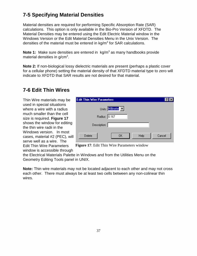
Thin Wire materials may beused in special situationswhere a wire with a radiusmuch smaller than the cellsize is required. Figure 17shows the window for editingthe thin wire radii in theWindows version. In mostcases, material #2 (PEC), willserve well as a wire. TheEdit Thin Wire Parameterswindow is accessible throughthe Electrical Materials Palette in Windows and from the Utilities Menu on theGeometry Editing Tools panel in UNIX.

Note: Thin wire materials may not be located adjacent to each other and may not crosseach other. There must always be at least two cells between any non-colinear thinwires.

38

Figure 18: Geometry Editing Tools (Windows Version)

Figure 19: Geometry Editing Tools in the Unix Version

7-7 Geometry Editing Tools

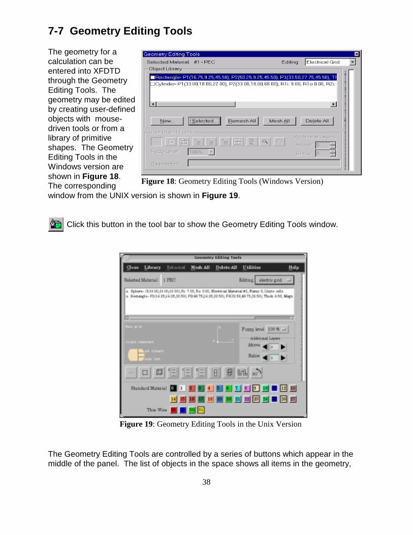
The geometry for acalculation can beentered into XFDTDthrough the GeometryEditing Tools. Thegeometry may be editedby creating user-definedobjects with mouse-driven tools or from alibrary of primitiveshapes. The GeometryEditing Tools in theWindows version areshown in Figure 18. The correspondingwindow from the UNIX version is shown in Figure 19.

Click this button in the tool bar to show the Geometry Editing Tools window.

The Geometry Editing Tools are controlled by a series of buttons which appear in themiddle of the panel. The list of objects in the space shows all items in the geometry,

39

Figure 20: Editing tools

whether they are meshed or not. If an object is meshed, the letter “m” will appear in thefirst column of the list. If it is unmeshed, the letter “u” will be displayed. The objects inthe list are meshed with items at the top of the list having priority over items at thebottom of the list. Items are added to the list at the top, so the last object added willhave the highest priority in meshing. The order of objects on the list can be change byclicking on an item in the list and then pressing Selected->Move (up/down/to top/tobottom). Other features of the “Selected” menu include meshing/unmeshing anddeleting an object from the list.

To add a new object to the list, press the New button and select one of the choices fromthe library or primitives. Each of the primitives is described later in this chapter. Afteradding the item to the list, it can be meshed by pressing the Mesh All button. If theorder of the items on the list has changed, the display of the mesh can be refreshed bypressing the Remsh All button. To clear the list of all objects, press the Delete Allbutton.

7-7-1 User-Defined Objects

A user-defined object can be created using the edit mode buttons (shown in Figure 20)which are for different manual (mouse-driven) editing modes. To create a user-definedobject, select Library->Begin user-defined (UNIX) or New->User Object (Windows) from the Geometry Editing Tools window. The edit mode buttons will then becomeavailable for use. There is also a spaceprovided for naming the user-defined objectfor future reference. Otherwise the object willappear on the list as simply “User Object”. The first three buttons are single-clickoperations. The first button sets single edges of cells. The second sets one face of acube while the third sets an entire cube directed normal to the viewing plane. The nextfive buttons allow definition of areas cells. The button labeled “X” will set only the X-directed components inside an area defined by the mouse. The “Y” and “Z” labeledbuttons function similarly. The button (with an icon of one square above another)draws two-dimensional “sheets” of cells in an area defined by the mouse. The editingbutton with the “two-cube” icon will set all geometry edges in the area selected. Thisincludes those components normal to the view. The last two buttons on the bar are forcopying an area and for rotating an area of cells. When finished, press Library->Enduser-defined (Unix) or End Object (Windows) to complete the user-defined object. When editing electric components, the dielectric material locations naturally align withthe grid. However, when placing magnetic components in the grid, the materiallocations are offset by ½ a cell in all directions. This convention is used to representthe locations for the electric and magnetic materials in the Yee cell geometry [7]. Thismay seem confusing when using the interactive mouse controlled editing of a magneticmesh, but it is easy to adapt to this.

40

Figure 21: Library menu

To aid in finding specific locations in the geometry, XFDTD displays the position of themouse pointer. In the Windows version the mouse pointer location is displayed on theright-most pane of the status bar. In the Unix Version the pointer location is drawn inthe upper right corner of the geometry window. As the pointer is moved in the geometrywindow, the location (in cells) is updated, including the orientation of the edge underthe pointer (X, Y, or Z). This position display is especially helpful in locating thevoltage and/or current sources and other geometry features. The material number ateach edge is also shown as the pointer is moved through the space.

7-7-2 Additional Layers in Geometry

For adding features to a User-defined object which extend through several layersabove and/or below the current viewing plane, the Edit Geometry Tools windowprovides the ability to duplicate editing actions through additional layers. This isaccomplished by setting the editing depth in the Additional Layers field. For example,if the view is set to the XY plane at Z=25, and the above editing depth is set to 5, thesame changes made in plane Z=25 will appear in planes Z=26 through Z=30. Thisgreatly simplifies the description of geometry shapes that have a constant cross sectionand extend over multiple layers of the space. The vertical bar on the right of the EditGeometry Tools window provides visual feedback of the editing characteristics.

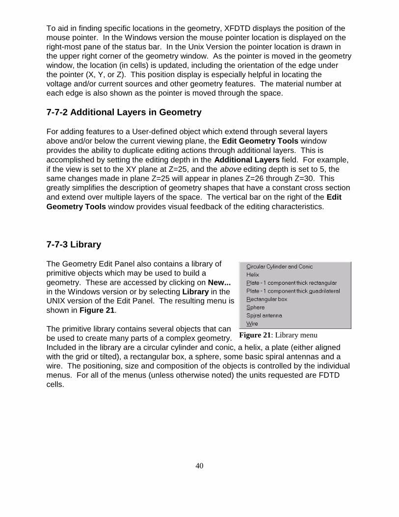
7-7-3 Library

The Geometry Edit Panel also contains a library ofprimitive objects which may be used to build ageometry. These are accessed by clicking on New...in the Windows version or by selecting Library in theUNIX version of the Edit Panel. The resulting menu isshown in Figure 21.

The primitive library contains several objects that canbe used to create many parts of a complex geometry. Included in the library are a circular cylinder and conic, a helix, a plate (either alignedwith the grid or tilted), a rectangular box, a sphere, some basic spiral antennas and awire. The positioning, size and composition of the objects is controlled by the individualmenus. For all of the menus (unless otherwise noted) the units requested are FDTDcells.

41

Figure 22: The circular cylinder andconic edit menu.

Figure 23: The helix primitive menu.

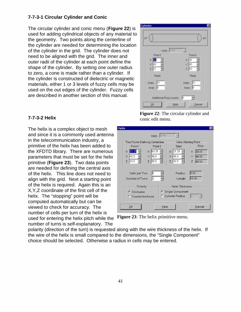
7-7-3-1 Circular Cylinder and Conic

The circular cylinder and conic menu (Figure 22) isused for adding cylindrical objects of any material tothe geometry. Two points along the centerline ofthe cylinder are needed for determining the locationof the cylinder in the grid. The cylinder does notneed to be aligned with the grid. The inner andouter radii of the cylinder at each point define theshape of the cylinder. By setting one outer radiusto zero, a cone is made rather than a cylinder. Ifthe cylinder is constructed of dielectric or magneticmaterials, either 1 or 3 levels of fuzzy cells may beused on the out edges of the cylinder. Fuzzy cellsare described in another section of this manual.

7-7-3-2 Helix

The helix is a complex object to meshand since it is a commonly used antennain the telecommunication industry, aprimitive of the helix has been added tothe XFDTD library. There are numerousparameters that must be set for the helixprimitive (Figure 23). Two data pointsare needed for defining the central axisof the helix. This line does not need toalign with the grid. Next a starting pointof the helix is required. Again this is anX,Y,Z coordinate of the first cell of thehelix. The “stopping” point will becomputed automatically but can beviewed to check for accuracy. Thenumber of cells per turn of the helix isused for entering the helix pitch while thenumber of turns is self-explanatory. Thepolarity (direction of the turn) is requested along with the wire thickness of the helix. Ifthe wire of the helix is small compared to the dimensions, the “Single Component”choice should be selected. Otherwise a radius in cells may be entered.

42

Figure 24: 1-component thickrectangular plate menu.

Figure 25: The quadrilateral platemenu.

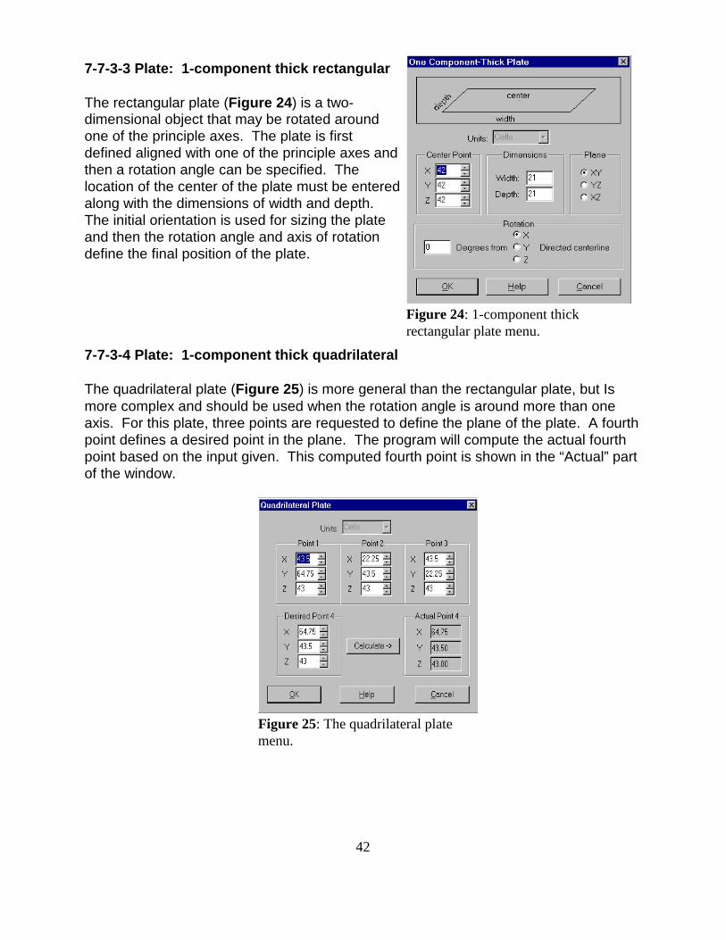
7-7-3-3 Plate: 1-component thick rectangular

The rectangular plate (Figure 24) is a two-dimensional object that may be rotated aroundone of the principle axes. The plate is firstdefined aligned with one of the principle axes andthen a rotation angle can be specified. Thelocation of the center of the plate must be enteredalong with the dimensions of width and depth. The initial orientation is used for sizing the plateand then the rotation angle and axis of rotationdefine the final position of the plate.

7-7-3-4 Plate: 1-component thick quadrilateral

The quadrilateral plate (Figure 25) is more general than the rectangular plate, but Ismore complex and should be used when the rotation angle is around more than oneaxis. For this plate, three points are requested to define the plane of the plate. A fourthpoint defines a desired point in the plane. The program will compute the actual fourthpoint based on the input given. This computed fourth point is shown in the “Actual” partof the window.

43

Figure 26: Rectangular Box menu

Figure 28: The spiral antenna primitivemenu.

Figure 27: The sphere primitivemenu.

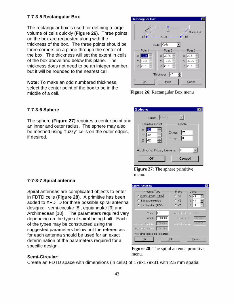
7-7-3-5 Rectangular Box

The rectangular box is used for defining a largevolume of cells quickly (Figure 26). Three pointson the box are requested along with thethickness of the box. The three points should bethree corners on a plane through the center ofthe box. The thickness will set the extent in cellsof the box above and below this plane. Thethickness does not need to be an integer number,but it will be rounded to the nearest cell.

Note: To make an odd numbered thickness,select the center point of the box to be in themiddle of a cell.

7-7-3-6 Sphere

The sphere (Figure 27) requires a center point andan inner and outer radius. The sphere may alsobe meshed using “fuzzy” cells on the outer edges,if desired.

7-7-3-7 Spiral antenna

Spiral antennas are complicated objects to enterin FDTD cells (Figure 28). A primitive has beenadded to XFDTD for three possible spiral antennadesigns: semi-circular [8], equiangular [9] andArchimedean [10]. The parameters required varydepending on the type of spiral being built. Eachof the types may be constructed using thesuggested parameters below but the referencesfor each antenna should be used for an exactdetermination of the parameters required for aspecific design.

Semi-Circular:Create an FDTD space with dimensions (in cells) of 178x179x31 with 2.5 mm spatial

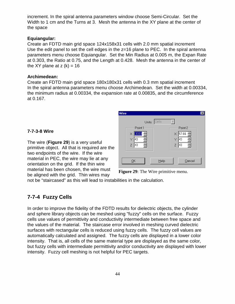
44

Figure 29: The Wire primitive menu.

increment. In the spiral antenna parameters window choose Semi-Circular. Set theWidth to 1 cm and the Turns at 3. Mesh the antenna in the XY plane at the center ofthe space

Equiangular:Create an FDTD main grid space 124x158x31 cells with 2.0 mm spatial incrementUse the edit panel to set the cell edges in the z=16 plane to PEC. In the spiral antennaparameters menu choose Equiangular. Set the Min Radius at 0.005 m, the Expan Rateat 0.303, the Ratio at 0.75, and the Length at 0.428. Mesh the antenna in the center ofthe XY plane at z (k) = 16

Archimedean:Create an FDTD main grid space 180x180x31 cells with 0.3 mm spatial incrementIn the spiral antenna parameters menu choose Archimedean. Set the width at 0.00334,the minimum radius at 0.00334, the expansion rate at 0.00835, and the circumferenceat 0.167.

7-7-3-8 Wire

The wire (Figure 29) is a very usefulprimitive object. All that is required are thetwo endpoints of the wire. If the wirematerial in PEC, the wire may lie at anyorientation on the grid. If the thin wirematerial has been chosen, the wire mustbe aligned with the grid. Thin wires maynot be “staircased” as this will lead to instabilities in the calculation.

7-7-4 Fuzzy Cells

In order to improve the fidelity of the FDTD results for dielectric objects, the cylinderand sphere library objects can be meshed using "fuzzy" cells on the surface. Fuzzycells use values of permittivity and conductivity intermediate between free space andthe values of the material. The staircase error involved in meshing curved dielectricsurfaces with rectangular cells is reduced using fuzzy cells. The fuzzy cell values areautomatically calculated and assigned. The fuzzy cells are displayed in a lower colorintensity. That is, all cells of the same material type are displayed as the same color,but fuzzy cells with intermediate permittivity and/or conductivity are displayed with lowerintensity. Fuzzy cell meshing is not helpful for PEC targets.

45

Figure 30: Change Spatial Increment window

While XFDTD automatically adjusts the relative permittivity on the surfaces of thesedielectric spheres and cylinders, the permittivity of flat surfaces of dielectric objects maybe adjusted manually. For this purpose a manual selection of Fuzzy levels is availablefrom the Edit Panel. If a cell is entirely within a dielectric material, fuzzy cells shouldnot be used. Note that if a cell is on the boundary between two dielectric materials, thecell is in effect halfway in one material and halfway in the other.

For example, consider the mesh edge locations tangent to a flat dielectric/air interface(at the surface of a dielectric substrate for example). The permittivity of these meshedges should be set to ( +1)/2 (the 1 for relative permittivity of free space) and theconductivity to /2, where and are the relative permittivity and conductivity inSiemens/meter of the dielectric. This corresponds to selecting the 50% Fuzzy levelfrom the edit menu for the dielectric at these surface mesh locations. If the adjoiningdielectric is not air, then the permittivity and conductivity are set to the average valuesof the two materials. In XFDTD it is assumed that the material is adjacent to air, and afuzzy level of x% means that the relative permittivity for that mesh location is set to[x +(100-x)]/100 and the conductivity is set to x /100. Other situations can beaccommodated by using a different dielectric material number for the intermediate“fuzzy” layer and setting its constitutive parameters appropriately.

This same correction should be applied to magnetic materials. Of course if theadjoining material is perfect conductor, then any electric fields tangent to the surface ofa perfect conductor are set as perfect conductor regardless of the constitutiveparameters of the adjoining material.

7-8 Spatial Increment

With the Change Spatial Incrementwindow the cell size of the cells in anFDTD geometry may be adjusted. (Figure30) This will not change the numbers orlocations of FDTD cells, only the cell size. This option should be used for makeadjustments or changes of scale. Remember than a 10x10 cell plate will stillbe 10x10 cells, but the actual dimensionin physical units will change based on thevalues entered on this window.

7-9 Add Dual Grid

Add Dual Grid may be used to add either the magnetic or electric grids to a geometry. In most circumstances this feature would be used if a geometry was defined with onlythe electric grid and at a later time some magnetic material was desired. By using thisfeature the dual grid will be added to the geometry and will be available for editing.

46

Adding the dual grid will increase the memory storage requirements of the geometrybecause three new three dimensional arrays will be added. Also the calculations of thefield equations by the calculation program will become slightly more complex. So, thedual grid should only be added when it is required.

Note that subgrids will not use magnetic materials in the FDTD calculations. Magneticmaterials may be defined in a subgrid geometry for cases where the subgrid will also beused as a main grid. However, any magnetic materials in a subgrid will be treated asfree space by the calculation program.

7-10 Preferences

The Preferences window allows control over numerous features of XFDTD. The valuesentered on the Preference window will be stored and used every time XFDTD is run inthe future.

The default units in both spatial and frequency terms may be modified to fit individualsituations. The options for frequency can range from Hertz to TeraHertz while spatialunits may be displayed in both metric or English values. XFDTD will use these units forany display of data.

Windows Version Preferences

The Windows version of XFDTD has some specialized preferences for controlling theappearance and function of XFDTD. The Interface preferences allows selection ofwhich windows in XFDTD are dockable. Dockable windows are those that can beattached to the sides of the main frame window. To dock a window, click and drag it tothe edge of the XFDTD frame window. The outline of the window will shrink when it willdock. To undock or float a window, double click on it, or drag the window off the frame. If windows are set as dockable, they may be moved without attaching by holding theControl key while moving.

The Material Palette section controls the display of materials on the material palette. Materials will be display either with the material descriptions entered, or by the materialnumber.

The XFDTD Project Tree section controls the behavior of the Project Tree. TheProject Tree can either display a text description for each item in the tree, or the actualfilename for that data.

The Quick Draw field display option controls how the field snapshots are drawn on thescreen. The fields may be drawn using the actual field values at each cell location, oran interpolated version of the fields may be shown which presents a smoother transitionof the fields. When Quick Draw is selected, the actual field values will be displayed

47

rather than the interpolated fields. The selection of Quick Draw will increase the speedin which fields are loaded and movies are presented.

The number of Undo levels for editing may be adjusted as well. The default setting forUndo is 2, but this can be increased as needed. The limitation on increasing thenumber of Undo levels is the memory requirement for storing changes to large areas ofthe geometry. When actions are stored in the undo list, the Information button willprovide an estimate of the amount of memory used.

48

8 View Menu

8-1 The View Menu in Windows XFDTD

Like the other menu items, the menu has different contents depending on which windowis currently active. View has different contents for depending whether the activewindow is a geometry, the run parameters, or a plot. The following items are commonregardless of which view is active:

� XFDTD Project Tree - Toggles the XFDTD Project tree. The Project Treedisplays all the files in the current project. Selecting items in the Project Treewill switch the geometry in view or open output files.

� Calculation Progress - Toggles the output window showing the status of anycalculation which may have been started.

� Tool Bar - Toggles the toolbar display. The toolbar is the row of buttons whichprovide instant access to various commonly used functions.

� Status Bar - Toggles the status bar located across the bottom of the XFDTDframe window. The Status Bar shows the file loading progress and the status ofother operations. More importantly, the status bar displays location of thepointer in a geometry as well as information about the active geometry.

The following items are only available when a geometry view is active:

U Grid - Toggles drawing of the grid. The grid is drawn as a medium-gray graphthat designates the size and position of the geometry. The drawing grid is inalignment with the electric components of the geometry.

U Normal Elements - Toggles the drawing of the components normal to thecurrent viewing plane. Normal components are drawn as circles in the color ofthe material. This setting is independent for each of the principle planar views.

U Electric Components - Toggles the drawing of the electric components. Whenboth an electric and magnetic grid are present, or when fields displayed, it issometimes useful to turn off the electric components. .

U Magnetic Components - Toggles the drawing of the magnetic components. U Background Color - This menu item controls the color of the geometry window

background. Note that the drawing background is switch to white for printingautomatically.

U Export .BMP - Exports the current view to a bitmap of a user-defined size. Thesize of the output bitmap must be entered followed by the filename.

8-2 The View Menu in Unix XFDTD

In the Unix version of XFDTD, the View menu does not change as there are notseparate windows for the Geometry and Run Parameters. The menu will appear asshown in Figure 31. The Hide Toolbar option removes the toolbar from the interface

49

Figure 31: The view menu in XFDTD 5.0 on aUnix computer.

window. Selecting this option again willreplace the toolbar. Use the Set ViewingSpace item to change which grid iscurrently in the view. The options forturning on and off the grid, normalelements, electrical components, andmagnetic components follow. Select 3DMode to view the geometry in threedimensions. Drawing Area Background isused to change the color of the geometrywindow.

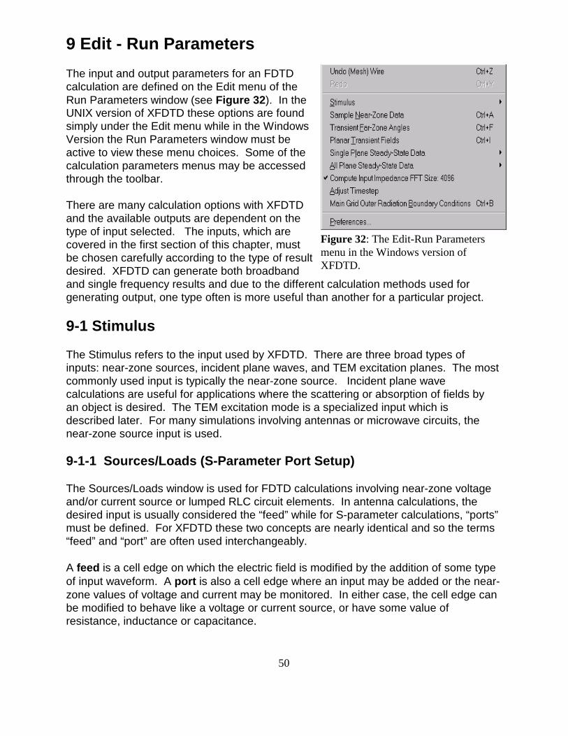
50

Figure 32: The Edit-Run Parametersmenu in the Windows version ofXFDTD.

9 Edit - Run Parameters

The input and output parameters for an FDTDcalculation are defined on the Edit menu of theRun Parameters window (see Figure 32). In theUNIX version of XFDTD these options are foundsimply under the Edit menu while in the WindowsVersion the Run Parameters window must beactive to view these menu choices. Some of thecalculation parameters menus may be accessedthrough the toolbar.

There are many calculation options with XFDTDand the available outputs are dependent on thetype of input selected. The inputs, which arecovered in the first section of this chapter, mustbe chosen carefully according to the type of resultdesired. XFDTD can generate both broadbandand single frequency results and due to the different calculation methods used forgenerating output, one type often is more useful than another for a particular project.

9-1 Stimulus

The Stimulus refers to the input used by XFDTD. There are three broad types ofinputs: near-zone sources, incident plane waves, and TEM excitation planes. The mostcommonly used input is typically the near-zone source. Incident plane wavecalculations are useful for applications where the scattering or absorption of fields byan object is desired. The TEM excitation mode is a specialized input which isdescribed later. For many simulations involving antennas or microwave circuits, thenear-zone source input is used.

9-1-1 Sources/Loads (S-Parameter Port Setup)

The Sources/Loads window is used for FDTD calculations involving near-zone voltageand/or current source or lumped RLC circuit elements. In antenna calculations, thedesired input is usually considered the “feed” while for S-parameter calculations, “ports”must be defined. For XFDTD these two concepts are nearly identical and so the terms“feed” and “port” are often used interchangeably.

A feed is a cell edge on which the electric field is modified by the addition of some typeof input waveform. A port is also a cell edge where an input may be added or the near-zone values of voltage and current may be monitored. In either case, the cell edge canbe modified to behave like a voltage or current source, or have some value ofresistance, inductance or capacitance.

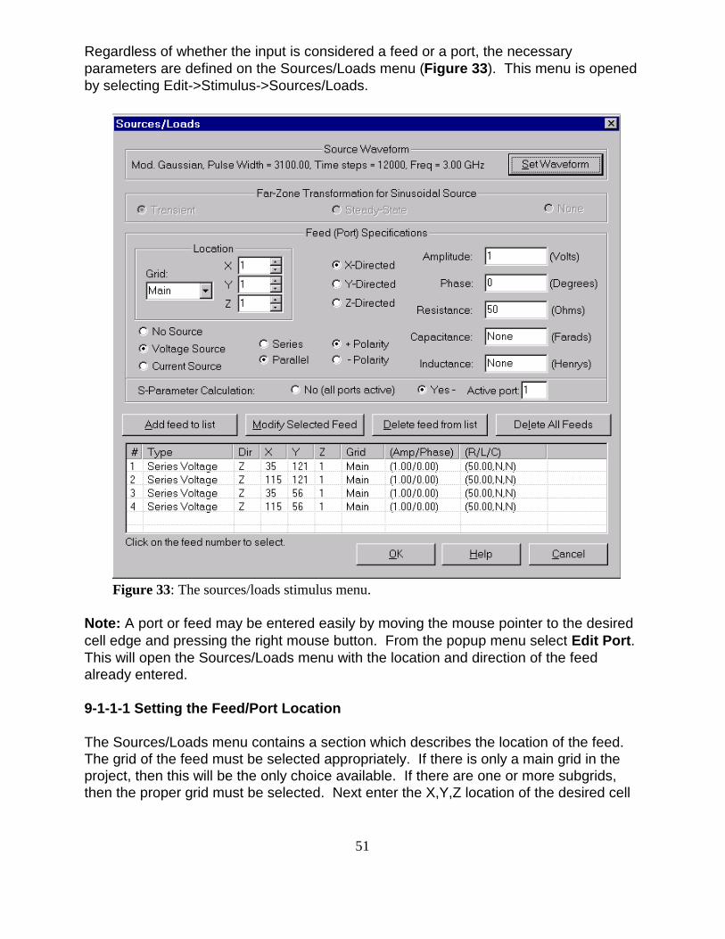
51

Figure 33: The sources/loads stimulus menu.

Regardless of whether the input is considered a feed or a port, the necessaryparameters are defined on the Sources/Loads menu (Figure 33). This menu is openedby selecting Edit->Stimulus->Sources/Loads.

Note: A port or feed may be entered easily by moving the mouse pointer to the desiredcell edge and pressing the right mouse button. From the popup menu select Edit Port. This will open the Sources/Loads menu with the location and direction of the feedalready entered.

9-1-1-1 Setting the Feed/Port Location

The Sources/Loads menu contains a section which describes the location of the feed. The grid of the feed must be selected appropriately. If there is only a main grid in theproject, then this will be the only choice available. If there are one or more subgrids,then the proper grid must be selected. Next enter the X,Y,Z location of the desired cell

52

edge. The feed will either be aligned with the X, Y or Z axes, so select the direction aseither “X-directed”, “Y-directed”, or “Z-directed”.

Note: Feeds/ports may not be located adjacent to each other unless the RLC valuesare all set to “none”. Feeds/Ports can be end-to-end, but the can not be side-by-side.

9-1-1-2 Feed/Port Parameters

Each port in XFDTD may have several parameters associated with it. The portcontains a source, the source may be a voltage or a current. The source may be addedin series or parallel. Otherwise, if no source is desired, a passive lumped load may bespecified by selecting No Source.

Note: For all voltage source specifications the values given are peak values, not RMS.

If a source is defined, the amplitude of the input waveform may be specified as well asthe polarity. The phase of the source may be selected if the input waveform is asinusoid, otherwise this option will be unavailable.

XFDTD also has the capability of simulating lumped RLC (Resistor/Inductor/Capacitor)elements at a port location. The RLC elements will be added either in series orparallel depending on which choice is selected. For all cases, the load will be in serieswith the voltage source and in parallel with the current source. The “series” and“parallel” choices refer to how the RLC components are added with respect to eachother. For the series combination, all of the lumped circuit elements are in series andare located on one FDTD mesh edge. For a parallel combination, all of the lumpedcircuit elements are in parallel located on one FDTD mesh edge. The voltage acrossthe mesh edge (electric field times edge length) includes both the load and the sourcevoltage (if present). The FDTD calculated current is always the total current throughthe cell edge and includes both current through the load and through the current source(if present).

If you wish to place a voltage source in parallel with the load or a current source inseries with the load, you should place the source and load in adjacent cells(side-by-side in the first case, and end-to-end in the second). The RLC values for thevoltage or current source should be set to “none” for this situation.

Source Resistance

An important advantage of including a source resistance is reducing the number ofFDTD time steps necessary for convergence in transient calculations. This isespecially important for resonant devices such as many antenna and microstrip circuits. With a "hard" source consisting of a voltage source without series resistance, aresonant microstrip antenna may require 64,000 time steps for the transients todissipate. The addition of a 50 ohm source resistance might reduce this to 4,000 timesteps. Similar time savings may be encountered for microwave circuits. The source

53

resistance should be chosen as closely as possible to match the source to what isbeing driven. So, for a microstrip problem with 50 ohm characteristic impedance asource resistance of 50 ohms would be a good choice. When making calculations that include the input voltage, current and/or power in thecalculation formula, such as antenna gain or S-Parameter values, the input voltage,current and/or power will be that provided at the terminals of the mesh edge. Inparticular, the power dissipated in the source/load resistor will not be included in theinput power. For example, the gain of antenna is reduced if any power is dissipated inlossy materials in the antenna, since this power is, therefore, not radiated. In XFDTD,since the voltage, current, and input power are calculated at the mesh edge, the gainof antenna will not be affected by the value of the source resistance. Similarly, for inputimpedance calculations, the source resistance, capacitance and inductance values willnot be included in the input impedance.

Note: The source resistance cannot be made too high or instability may result. In thesource resistance calculation the displacement (capacitive) current through the FDTDcell is neglected. If the source resistance is made high enough so that the neglecteddisplacement current become larger than the conduction current through the sourceresistance, Maxwell’s equations will not be satisfied and the FDTD calculation may gounstable.

9-1-1-3 Modifying Feed/Port Parameters

If a feed location was entered incorrectly, or it has moved, the entry may be editedsimply by follow the procedure below.

1) Select the feed from the list.

2) Make the desired changes to the Feed Specifications. While the changes are beingmade, the selected feed will remain highlighted.

3) Click on Modify Selected Feed to replace the selected feed with the newspecifications.

9-1-1-4 Multiple Voltage and/or Current Sources

For calculations with multiple voltage and/or current sources, such as antenna arrays ormulti-port S-parameter calculations, multiple feed points can be specified with theSources/Loads window. For transient feeds, each source function must have the samepulse width and amplitude, or use the same user supplied file of voltage versus time. The polarity can be adjusted by clicking the desired button. This may be useful incontrolling the sign of the phase terms in S-parameter calculations. For each feed,independent source resistances may be specified. For sinusoidal excitations, eachfeed can be specified with a different magnitude and phase.

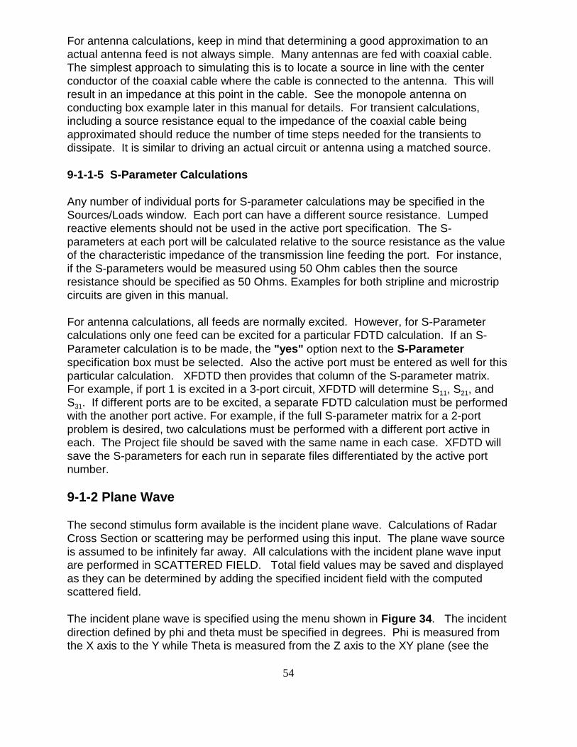
54

For antenna calculations, keep in mind that determining a good approximation to anactual antenna feed is not always simple. Many antennas are fed with coaxial cable. The simplest approach to simulating this is to locate a source in line with the centerconductor of the coaxial cable where the cable is connected to the antenna. This willresult in an impedance at this point in the cable. See the monopole antenna onconducting box example later in this manual for details. For transient calculations,including a source resistance equal to the impedance of the coaxial cable beingapproximated should reduce the number of time steps needed for the transients todissipate. It is similar to driving an actual circuit or antenna using a matched source.

9-1-1-5 S-Parameter Calculations

Any number of individual ports for S-parameter calculations may be specified in theSources/Loads window. Each port can have a different source resistance. Lumpedreactive elements should not be used in the active port specification. The S-parameters at each port will be calculated relative to the source resistance as the valueof the characteristic impedance of the transmission line feeding the port. For instance,if the S-parameters would be measured using 50 Ohm cables then the sourceresistance should be specified as 50 Ohms. Examples for both stripline and microstripcircuits are given in this manual.

For antenna calculations, all feeds are normally excited. However, for S-Parametercalculations only one feed can be excited for a particular FDTD calculation. If an S-Parameter calculation is to be made, the "yes" option next to the S-Parameterspecification box must be selected. Also the active port must be entered as well for thisparticular calculation. XFDTD then provides that column of the S-parameter matrix. For example, if port 1 is excited in a 3-port circuit, XFDTD will determine S11, S21, andS31. If different ports are to be excited, a separate FDTD calculation must be performedwith the another port active. For example, if the full S-parameter matrix for a 2-portproblem is desired, two calculations must be performed with a different port active ineach. The Project file should be saved with the same name in each case. XFDTD willsave the S-parameters for each run in separate files differentiated by the active portnumber.

9-1-2 Plane Wave

The second stimulus form available is the incident plane wave. Calculations of RadarCross Section or scattering may be performed using this input. The plane wave sourceis assumed to be infinitely far away. All calculations with the incident plane wave inputare performed in SCATTERED FIELD. Total field values may be saved and displayedas they can be determined by adding the specified incident field with the computedscattered field.

The incident plane wave is specified using the menu shown in Figure 34. The incidentdirection defined by phi and theta must be specified in degrees. Phi is measured fromthe X axis to the Y while Theta is measured from the Z axis to the XY plane (see the

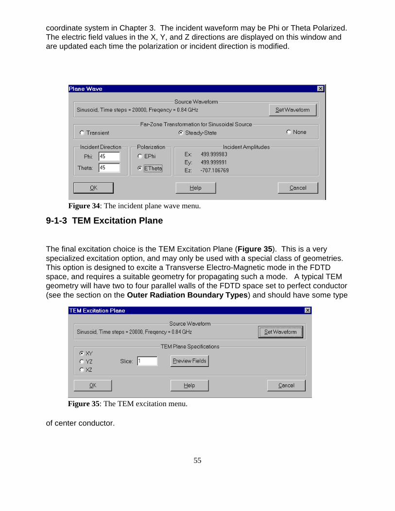
55

Figure 34: The incident plane wave menu.

Figure 35: The TEM excitation menu.

coordinate system in Chapter 3. The incident waveform may be Phi or Theta Polarized. The electric field values in the X, Y, and Z directions are displayed on this window andare updated each time the polarization or incident direction is modified.

9-1-3 TEM Excitation Plane

The final excitation choice is the TEM Excitation Plane (Figure 35). This is a veryspecialized excitation option, and may only be used with a special class of geometries. This option is designed to excite a Transverse Electro-Magnetic mode in the FDTDspace, and requires a suitable geometry for propagating such a mode. A typical TEMgeometry will have two to four parallel walls of the FDTD space set to perfect conductor(see the section on the Outer Radiation Boundary Types) and should have some type

of center conductor.

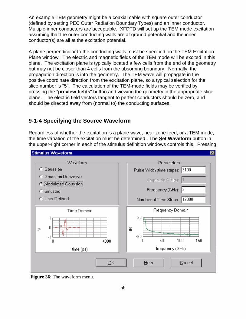
56

Figure 36: The waveform menu.

An example TEM geometry might be a coaxial cable with square outer conductor(defined by setting PEC Outer Radiation Boundary Types) and an inner conductor. Multiple inner conductors are acceptable. XFDTD will set up the TEM mode excitationassuming that the outer conducting walls are at ground potential and the innerconductor(s) are all at the excitation potential.

A plane perpendicular to the conducting walls must be specified on the TEM ExcitationPlane window. The electric and magnetic fields of the TEM mode will be excited in thisplane. The excitation plane is typically located a few cells from the end of the geometrybut may not be closer than 4 cells from the absorbing boundary. Normally, thepropagation direction is into the geometry. The TEM wave will propagate in thepositive coordinate direction from the excitation plane, so a typical selection for theslice number is "5". The calculation of the TEM-mode fields may be verified bypressing the "preview fields" button and viewing the geometry in the appropriate sliceplane. The electric field vectors tangent to perfect conductors should be zero, andshould be directed away from (normal to) the conducting surfaces.

9-1-4 Specifying the Source Waveform

Regardless of whether the excitation is a plane wave, near zone feed, or a TEM mode,the time variation of the excitation must be determined. The Set Waveform button inthe upper-right corner in each of the stimulus definition windows controls this. Pressing

57

Frequency ï

1

10 t 3

'

c

10 x

the Set Waveform button brings up this window. (Figure 36)

The excitation for the FDTD calculation may be a Gaussian pulse, a GaussianDerivative pulse, a Modulated Gaussian pulse, a Sinusoid, or “user defined” in whichcase a custom waveform may be supplied. The choice of the excitation should bebased on the desired output results as some excitations are more appropriate thanothers. The Gaussian pulse provides a broadband input and is suitable when resultsversus frequency are desired. The derivative Gaussian is nearly identical to theGaussian except that the DC component is removed. This is useful for calculationswhere a short-circuit loop exists since the regular Gaussian could excite DC currentflow which would affect the quality of the output. The modulated Gaussian is usedwhen only a specific frequency range is desired. This is very useful in structures wherelow frequencies could excite non-radiating modes which could resonate and destroy theresults. The sinusoidal input is useful when only one frequency is of interest. Thereare numerous output choices available with the sinusoidal input as well.

Depending on which waveform chosen, the appropriate parameters of the excitation areavailable for selection. The pulse width is the number of timesteps between the half-amplitude points on the Gaussian pulse input. For a Gaussian modulated pulse thereis a Gaussian envelope of the specified pulse width enclosing a sine wave of thespecified frequency. The sine wave is centered in the Gaussian envelope so that theaverage value of the pulse is zero. The two graphs in this window show the timevariation and frequency spectrum of the waveform to aid in correctly specifying theparameters.

When choosing the pulse width and/or frequency, bear in mind the constraints of theFDTD method. The time rate of change of the pulse (maximum frequency withsignificant energy) or the sine wave frequency must be chosen low enough so that asufficient number of time steps occur during one period for reasonably accuratesampling. The Courant limit for the time step size is where x is the size of the celledge, t is the time step, and c is the speed of light. Assuming the often appliedconstraint that x< /10, the maximum frequency specified is then constrained by:

The default size for the Gaussian pulse width is 32 time steps. This provides areasonable frequency bandwidth for the Gaussian pulse. For the Gaussian derivativepulse the time duration should be set somewhat greater since the Gaussian derivativepulse will have a higher frequency spectrum than a Gaussian pulse of the same timeduration.

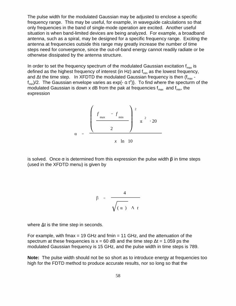
58

'

fmax

& fmin

2

2

2@ 20

x ln 10

'

4

( ) t

The pulse width for the modulated Gaussian may be adjusted to enclose a specificfrequency range. This may be useful, for example, in waveguide calculations so that only frequencies in the band of single-mode operation are excited. Another usefulsituation is when band-limited devices are being analyzed. For example, a broadbandantenna, such as a spiral, may be designed for a specific frequency range. Exciting theantenna at frequencies outside this range may greatly increase the number of timesteps need for convergence, since the out-of-band energy cannot readily radiate or beotherwise dissipated by the antenna structure.

In order to set the frequency spectrum of the modulated Gaussian excitation fmax isdefined as the highest frequency of interest (in Hz) and fmin as the lowest frequency,and t the time step. In XFDTD the modulated Gaussian frequency is then (fmax -fmin)/2. The Gaussian envelope varies as exp{- t2)}. To find where the specturm of themodulated Gaussian is down x dB from the pak at frequencies fmax and fmin, theexpression

is solved. Once is determined from this expression the pulse width in time steps(used in the XFDTD menu) is given by

where t is the time step in seconds.

For example, with fmax = 19 GHz and fmin = 11 GHz, and the attenuation of thespectrum at these frequencies is x = 60 dB and the time step t = 1.059 ps themodulated Gaussian frequency is 15 GHz, and the pulse width in time steps is 789.

Note: The pulse width should not be so short as to introduce energy at frequencies toohigh for the FDTD method to produce accurate results, nor so long so that the

59

calculation is not excited at frequencies for which accurate and useful results might beobtained. There must be sufficient energy in the pulse for calculations to be above thenumerical noise for all frequencies of interest. For calculations with very small cellscompared to the shortest wavelength of interest, pulse widths may be set much largerthan the default size to reduce the number of time steps needed for convergence and toincrease stability.

If dielectric materials are present, the wavelength will be reduced inside the materialand the velocity of propagation will be less than the speed of light in free space. Areasonable rule to apply is that the maximum frequency for the spectrum of theexcitation pulse should be reduced by the square root of the relative permittivity, orequivalently the pulse width should be increased by this factor. This assumes losslessor low loss dielectric. For more lossy dielectrics or conductors, the frequency and pulsewidth should be adjusted proportionally to the change in velocity and wavelength in thematerial relative to the free space wavelength. Of course the maximum frequency forreliable results is also reduced as the frequency spectrum of the excitation pulse isreduced.

For example, suppose part of the calculation space is free space and part is a low lossdielectric with relative permittivity 4.0 Further suppose the cell size is 1 cm. At 10 cellsper wavelength, one would expect reasonable results up to 3 GHz with a Gaussianpulse 32 time steps wide. But since part of the space has the dielectric material, withthe same cell size the Gaussian pulse width should be increased to 64 to reduce thefrequency spectrum bandwidth. Correspondingly, the maximum frequency for reliableresults would be decreased from 3 to 1.5 GHz.

Note: When the pulse width is changed from the default values, the FDTD results forsome frequencies will not be valid since the energy spectrum of the modified pulse willnot excite the problem over then entire spectrum. When displaying such results limitthe frequency range accordingly.

When choosing the source form, remember that the Gaussian pulse has a non-zeroaverage value. It should not be used for calculations if there is a closed path (loop) ofperfect conductor connected to the electric field location unless a source resistance isalso specified. This is because a steady current will start to flow in the loop and neverdecay through loss or radiation. The symptom of this will be a source current that hasan average value not equal to zero. If this occurs, the Gaussian Derivative orModulated Gaussian pulses can be used or a non-zero source resistance included inthe calculation.

An arbitrary source voltage vs time my be specified by choosing User Defined from theStimulus Waveform window. Pressing this option will open a menu asking for theinput filename with an extension .src. The file format for a user-defined waveform isas follows: the first line must be an integer which is the number of time steps in thewaveform, additional timesteps will be zero-padded. The format of the rest of the filedepends upon whether a voltage source or incident plane wave calculation is being

60

made. For a voltage source excitation each following line, one for each time step,contains two floating point number representing the voltage and its time derivative atthe feed at that timestep. For an incident plane wave calculation, each following line,one for each time step, contains two floating point numbers. The first number on eachline is the electric field value, in Volts/meter, at each time step, and the second is thetime derivative of the electric field of the incident plane wave.

9-1-5 Number of Time Steps

For each of the different types of Stimulus, a number of time steps for the FDTDcalculation must be specified. This number must be chosen with care since a lownumber will terminate the calculation before convergence of the results is obtained. Ahigh number will cause unnecessary calculations to be performed, but will not result inerrors. XFDTD will display an error message if the number of timesteps entered is toosmall to include the input waveform, but this number is far lower than the actual numberof timesteps required by the calculation.

For a transient calculation, the number of timesteps should be large enough for allfields to decay to zero. This can be checked by making a calculation and observing thetransient field results by sampling near-zone field points. For a sinusoidal excitation,sufficient time steps to reach steady-state must be chosen. Again, near-zone valuesshould be saved and observed so ensure that the system has reached steady-state.

Results that require the application of an FFT (any results which will be displayedversus frequency), or that assume steady-state sine wave conditions have beenreached (such as antenna efficiency or steady-state far-zone transformation) will not beaccurate if sufficient time steps to not been specified. It is vital that the near-zoneresults be observed to determine convergence before attempting to make conclusionsabout the output of a calculation.

Note: The only way to be ensured of convergence of the FDTD calculation is to viewthe time records of near-zone field values or the feed point current/voltage. XFDTDdoes not send an error message when an insufficient number of timesteps have beencalculation. The determination of convergence or steady-state is left up to the user andis best viewed by plotting near-zone field values.

9-1-6 Far Zone Transformation for a Sinusoidal Source

In the Sources/Loads and Plane Wave Run Parameter sub-menus there is a choice forthe Far-zone transformation type for a sinusoidal input (Figure 33). If a transient input(gaussian pulse etc) is chosen, this option will not be available. The choices for the far-zone transform are between Transient, Steady-State, or None. Typically this optionshould be selected as “Steady-State” since this offers the most flexibility. However, ifonly near-zone values are of interest such as in an S-parameter or SAR calculation,selecting “None” will save a small amount of calculation time and a sizable amount ofdisk space. In some instances, the transient far-zone calculation may be desired and

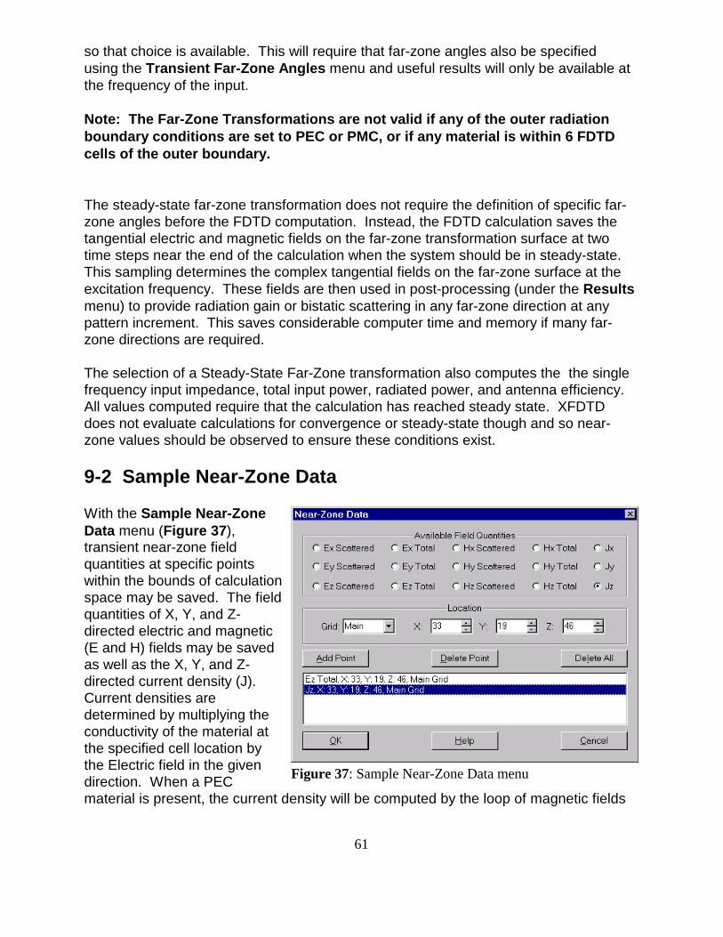
61

Figure 37: Sample Near-Zone Data menu

so that choice is available. This will require that far-zone angles also be specifiedusing the Transient Far-Zone Angles menu and useful results will only be available atthe frequency of the input.

Note: The Far-Zone Transformations are not valid if any of the outer radiationboundary conditions are set to PEC or PMC, or if any material is within 6 FDTDcells of the outer boundary.

The steady-state far-zone transformation does not require the definition of specific far-zone angles before the FDTD computation. Instead, the FDTD calculation saves thetangential electric and magnetic fields on the far-zone transformation surface at twotime steps near the end of the calculation when the system should be in steady-state. This sampling determines the complex tangential fields on the far-zone surface at theexcitation frequency. These fields are then used in post-processing (under the Resultsmenu) to provide radiation gain or bistatic scattering in any far-zone direction at anypattern increment. This saves considerable computer time and memory if many far-zone directions are required.

The selection of a Steady-State Far-Zone transformation also computes the the singlefrequency input impedance, total input power, radiated power, and antenna efficiency. All values computed require that the calculation has reached steady state. XFDTDdoes not evaluate calculations for convergence or steady-state though and so near-zone values should be observed to ensure these conditions exist.

9-2 Sample Near-Zone Data

With the Sample Near-ZoneData menu (Figure 37),transient near-zone fieldquantities at specific pointswithin the bounds of calculationspace may be saved. The fieldquantities of X, Y, and Z-directed electric and magnetic(E and H) fields may be savedas well as the X, Y, and Z-directed current density (J). Current densities aredetermined by multiplying theconductivity of the material atthe specified cell location bythe Electric field in the givendirection. When a PECmaterial is present, the current density will be computed by the loop of magnetic fields

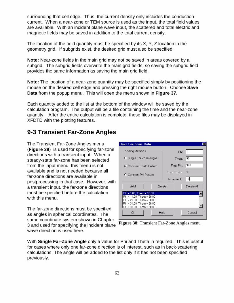
62

Figure 38: Transient Far-Zone Angles menu

surrounding that cell edge. Thus, the current density only includes the conductioncurrent. When a near-zone or TEM source is used as the input, the total field valuesare available. With an incident plane wave input, the scattered and total electric andmagnetic fields may be saved in addition to the total current density.

The location of the field quantity must be specified by its X, Y, Z location in thegeometry grid. If subgrids exist, the desired grid must also be specified.

Note: Near-zone fields in the main grid may not be saved in areas covered by asubgrid. The subgrid fields overwrite the main grid fields, so saving the subgrid fieldprovides the same information as saving the main grid field.

Note: The location of a near-zone quantity may be specified simply by positioning themouse on the desired cell edge and pressing the right mouse button. Choose SaveData from the popup menu. This will open the menu shown in Figure 37.

Each quantity added to the list at the bottom of the window will be saved by thecalculation program. The output will be a file containing the time and the near-zonequantity. After the entire calculation is complete, these files may be displayed inXFDTD with the plotting features.

9-3 Transient Far-Zone Angles

The Transient Far-Zone Angles menu(Figure 38) is used for specifying far-zonedirections with a transient input. When asteady-state far-zone has been selectedfrom the input menu, this menu is notavailable and is not needed because allfar-zone directions are available inpostprocessing in that case. However, witha transient input, the far-zone directionsmust be specified before the calculationwith this menu.

The far-zone directions must be specifiedas angles in spherical coordinates. Thesame coordinate system shown in Chapter3 and used for specifying the incident planewave direction is used here.

With Single Far-Zone Angle only a value for Phi and Theta in required. This is usefulfor cases where only one far-zone direction is of interest, such as in back-scatteringcalculations. The angle will be added to the list only if it has not been specifiedpreviously.

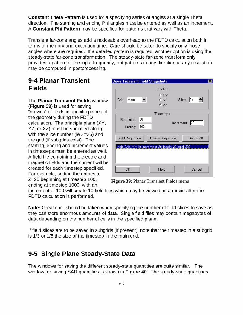
63

Figure 39: Planar Transient Fields menu

Constant Theta Pattern is used for a specifying series of angles at a single Thetadirection. The starting and ending Phi angles must be entered as well as an increment. A Constant Phi Pattern may be specified for patterns that vary with Theta.

Transient far-zone angles add a noticeable overhead to the FDTD calculation both interms of memory and execution time. Care should be taken to specify only thoseangles where are required. If a detailed pattern is required, another option is using thesteady-state far-zone transformation. The steady-state far-zone transform onlyprovides a pattern at the input frequency, but patterns in any direction at any resolutionmay be computed in postprocessing.

9-4 Planar TransientFields

The Planar Transient Fields window(Figure 39) is used for saving“movies” of fields in specific planes ofthe geometry during the FDTDcalculation. The principle plane (XY,YZ, or XZ) must be specified alongwith the slice number (ie Z=25) andthe grid (if subgrids exist). Thestarting, ending and increment valuesin timesteps must be entered as well. A field file containing the electric andmagnetic fields and the current will becreated for each timestep specified. For example, setting the entries toZ=25 beginning at timestep 100,ending at timestep 1000, with anincrement of 100 will create 10 field files which may be viewed as a movie after theFDTD calculation is performed.

Note: Great care should be taken when specifying the number of field slices to save asthey can store enormous amounts of data. Single field files may contain megabytes ofdata depending on the number of cells in the specified plane.

If field slices are to be saved in subgrids (if present), note that the timestep in a subgridis 1/3 or 1/5 the size of the timestep in the main grid.

9-5 Single Plane Steady-State Data

The windows for saving the different steady-state quantities are quite similar. Thewindow for saving SAR quantities is shown in Figure 40. The steady-state quantities

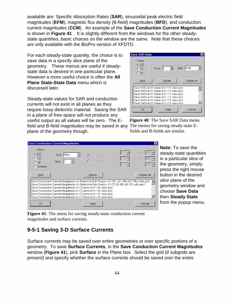
64

Figure 40: The Save SAR Data menu. The menus for saving steady-state E-fields and B-fields are similar.

Figure 41: The menu for saving steady-state conduction currentmagnitudes and surface currents.

available are: Specific Absorption Rates (SAR), sinusoidal peak electric fieldmagnitudes (EFM), magnetic flux density (B-field) magnitudes (BFD), and conductioncurrent magnitudes (CCM). An example of the Save Conduction Current Magnitudesis shown in Figure 41 . It is slightly different from the windows for the other steady-state quantities, basic choices on the window are the same. Note that these choicesare only available with the BioPro version of XFDTD.

For each steady-state quantity, the choice is tosave data in a specify slice plane of thegeometry. These menus are useful if steady-state data is desired in one particular plane. However a more useful choice is often the AllPlane State-State Data menu which isdiscussed later.

Steady-state values for SAR and conductioncurrents will not exist in all planes as theyrequire lossy dielectric material. Saving the SARin a plane of free-space will not produce anyuseful output as all values will be zero. The E-field and B-field magnitudes may be saved in anyplane of the geometry though.

Note: To save thesteady-state quantitiesin a particular slice ofthe geometry, simplypress the right mousebutton in the desiredslice plane of thegeometry window andchoose Save Datathen Steady Statefrom the popup menu.

9-5-1 Saving 3-D Surface Currents

Surface currents may be saved over entire geometries or over specific portions of ageometry. To save Surface Currents, in the Save Conduction Current Magnitudeswindow (Figure 41), pick Surface in the Plane box. Select the grid (if subgrids arepresent) and specify whether the surface currents should be saved over the entire

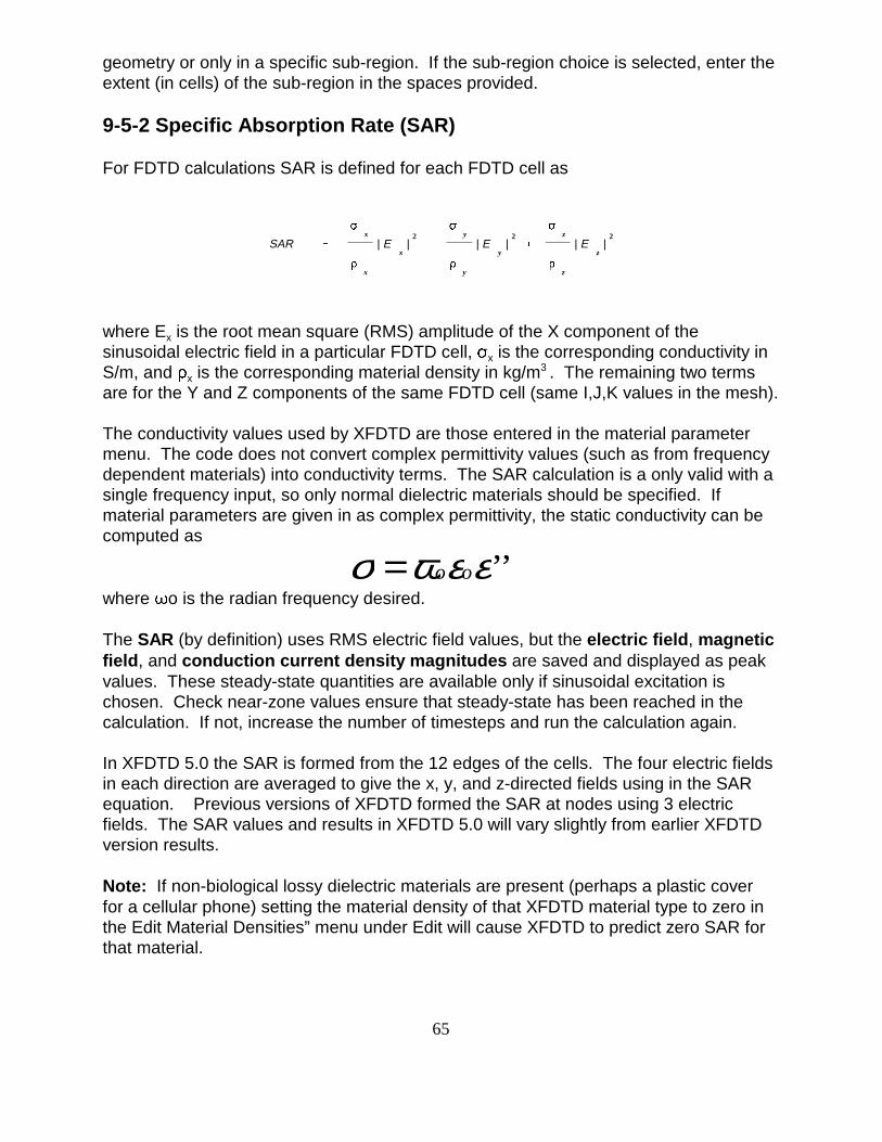
65

SAR '

x

x

| Ex

|2%

y

y

| Ey

|2%

z

z

| Ez

|2

geometry or only in a specific sub-region. If the sub-region choice is selected, enter theextent (in cells) of the sub-region in the spaces provided.

9-5-2 Specific Absorption Rate (SAR)

For FDTD calculations SAR is defined for each FDTD cell as

where Ex is the root mean square (RMS) amplitude of the X component of thesinusoidal electric field in a particular FDTD cell, x is the corresponding conductivity inS/m, and x is the corresponding material density in kg/m3 . The remaining two termsare for the Y and Z components of the same FDTD cell (same I,J,K values in the mesh).

The conductivity values used by XFDTD are those entered in the material parametermenu. The code does not convert complex permittivity values (such as from frequencydependent materials) into conductivity terms. The SAR calculation is a only valid with asingle frequency input, so only normal dielectric materials should be specified. Ifmaterial parameters are given in as complex permittivity, the static conductivity can becomputed as

σ ωε ε= o o ’’where o is the radian frequency desired.

The SAR (by definition) uses RMS electric field values, but the electric field, magneticfield, and conduction current density magnitudes are saved and displayed as peakvalues. These steady-state quantities are available only if sinusoidal excitation ischosen. Check near-zone values ensure that steady-state has been reached in thecalculation. If not, increase the number of timesteps and run the calculation again.

In XFDTD 5.0 the SAR is formed from the 12 edges of the cells. The four electric fieldsin each direction are averaged to give the x, y, and z-directed fields using in the SARequation. Previous versions of XFDTD formed the SAR at nodes using 3 electricfields. The SAR values and results in XFDTD 5.0 will vary slightly from earlier XFDTDversion results.

Note: If non-biological lossy dielectric materials are present (perhaps a plastic coverfor a cellular phone) setting the material density of that XFDTD material type to zero inthe Edit Material Densities” menu under Edit will cause XFDTD to predict zero SAR forthat material.

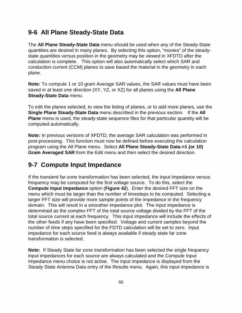
66

9-6 All Plane Steady-State Data

The All Plane Steady-State Data menu should be used when any of the Steady-Statequantities are desired in many planes. By selecting this option, “movies” of the steady-state quantities versus position in the geometry may be viewed in XFDTD after thecalculation is complete. This option will also automatically select which SAR andconduction current (CCM) planes to save based the material in the geometry in eachplane.

Note: To compute 1 or 10 gram Average SAR values, the SAR values must have beensaved in at least one direction (XY, YZ, or XZ) for all planes using the All PlaneSteady-State Data menu.

To edit the planes selected, to view the listing of planes, or to add more planes, use the Single Plane Steady-State Data menu described in the previous section. If the AllPlane menu is used, the steady-state sequence files for that particular quantity will becomputed automatically.

Note: In previous versions of XFDTD, the average SAR calculation was performed inpost-processing. This function must now be defined before executing the calculationprogram using the All Plane menu. Select All Plane Steady-State Data->1 (or 10)Gram Averaged SAR from the Edit menu and then select the desired direction.

9-7 Compute Input Impedance

If the transient far-zone transformation has been selected, the input impedance versusfrequency may be computed for the first voltage source. To do this, select theCompute Input Impedance option (Figure 42). Enter the desired FFT size on themenu which must be larger than the number of timesteps to be computed. Selecting a larger FFT size will provide more sample points of the impedance in the frequencydomain. This will result in a smoother impedance plot. The input impedance isdetermined as the complex FFT of the total source voltage divided by the FFT of thetotal source current at each frequency. This input impedance will include the effects ofthe other feeds if any have been specified. Voltage and current samples beyond thenumber of time steps specified for the FDTD calculation will be set to zero. Inputimpedance for each source feed is always available if steady state far zonetransformation is selected.

Note: If Steady State far zone transformation has been selected the single frequencyinput impedances for each source are always calculated and the Compute InputImpedance menu choice is not active. The input impedance is displayed from theSteady State Antenna Data entry of the Results menu. Again, this input impedance is

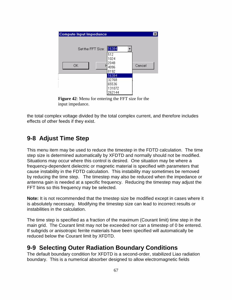
67

Figure 42: Menu for entering the FFT size for theinput impedance.

the total complex voltage divided by the total complex current, and therefore includeseffects of other feeds if they exist.

9-8 Adjust Time Step

This menu item may be used to reduce the timestep in the FDTD calculation. The timestep size is determined automatically by XFDTD and normally should not be modified. Situations may occur where this control is desired. One situation may be where afrequency-dependent dielectric or magnetic material is specified with parameters thatcause instability in the FDTD calculation. This instability may sometimes be removedby reducing the time step. The timestep may also be reduced when the impedance orantenna gain is needed at a specific frequency. Reducing the timestep may adjust theFFT bins so this frequency may be selected.

Note: It is not recommended that the tmestep size be modified except in cases where itis absolutely necessary. Modifying the timestep size can lead to incorrect results orinstabilities in the calculation.

The time step is specified as a fraction of the maximum (Courant limit) time step in themain grid. The Courant limit may not be exceeded nor can a timestep of 0 be entered. If subgrids or anisotropic ferrite materials have been specified will automatically bereduced below the Courant limit by XFDTD.

9-9 Selecting Outer Radiation Boundary ConditionsThe default boundary condition for XFDTD is a second-order, stabilized Liao radiationboundary. This is a numerical absorber designed to allow electromagnetic fields

68

Figure 43: The menu for setting the outer radiationboundary condition.

radiated or scattered by the FDTD geometry to be absorbed with very little reflectionfrom the boundary. The Perfectly Matched Layers (PML) outer boundary is alsoavailable (see Figure 43). The Liao and PML boundaries may not be mixed together inthe same calculation. Furthermore, PML may not be used with the Perfect MagneticConductor (PMC) boundary, while Liao may be used with both Perfect ElectricalConductor (PEC) and PMC boundaries.

Note: XFDTD treats the specificationof the outer boundary as acalculation parameter, not ageometry feature. Thus the outerboundary specification is stored inthe XFDTD project file, not in thegeometry file. A conducting outerboundary will not be evident in thegeometry view until the project filehas been loaded.

9-9-1 Liao Absorbing Boundary Type

It is important to understand the differences between the Liao and PML options. Liao isan estimation method. By looking into the FDTD space and back in time it estimates theelectric fields just outside the limits of the FDTD mesh. These estimated values arethen used in the FDTD equations inside the space. The Liao estimation is madeassuming that waves are allowed to travel outwardly from the space but not reflect backin. The Liao method works well provided that there is enough space between theradiating geometry and the outer boundary. Typical limits are at least 15 cells spacing.

A homogeneous dielectric may be located up against the Liao boundary. For example,in a lossy earth or stripline calculation, the earth or dielectric layer may touch the outerboundary. Liao will usually function well in this situation, provided that there are no airgaps within 5 cells of the Liao boundary. Liao assumes homogeneous material within 5cells, and if this is not the case then the FDTD calculation will usually be unstable withrapidly rising field amplitudes.

69

Since Liao is an estimation method, the size of the FDTD mesh is not increased byusing it. Some storage is needed for saving electric values at previous time steps, butthis is usually negligible in a typical calculation.

9-9-2 PML Absorbing Boundary Type

PML is an artificial absorbing material. It absorbs the incident energy as it propagatesthrough the PML layers. Better absorption, that is, smaller reflection, is obtained byadding more layers at the expense of increasing the size of the FDTD mesh. Forexample, consider an FDTD calculation on a mesh using the Liao absorber that is 50 x60 x 70 cells or a total of 210,000 cells. There is a 15 cell free space border all aroundthe geometry so that the Liao boundaries can provide small reflections. If the Liao ischanged to 8 PML layers, the geometry mesh will not change However outside of thisdefined mesh region, 8 additional FDTD mesh layers are added on each side of thegeometry. This means that the actual number of FDTD cells that must be calculatedgrows to 66 x 76 x 86 or 431,000 cells, more than double. Since PML cells requiremore arithmetic operations than normal FDTD cells, the time penalty is actually greater.

This time penalty for PML is also increased since the PML cells have special equationsfor both electric and magnetic fields. For an FDTD calculation with no magneticmaterials present the magnetic fields are computed very quickly. However, when PMLis added the magnetic field update equations are more complicated even when noactual magnetic fields are present and this adds to the time penalty.

Benefits of PML

It may be that the PML layers might provide better absorption than Liao even with onlya 5 cell border of free space. And perhaps only 6 PML layers would provide this. So insuch a situation calculation time would be saved. Making this comparison wouldrequire meshing the object again with less free space margin to the outer boundary. This can be done in XFDTD using the mesh merge function.

Both PML and Liao are offered to provide flexibility. Both methods should providesimilar results when properly used.

9-9-3 PEC (Perfect Electric Conductor)

Radiation and scattering calculations require that all six outer boundaries be set asabsorbing. In some situations there are advantages terminating one or more faces ofthe FDTD geometry space with a perfect electric conductor (PEC). For example. theconducting ground plane of a microstrip could be located on one face of the FDTDspace.

70

A special utilization of this capability involves setting four of the FDTD surfaces to PECforming a rectangular conducting tube. These may be considered as the outer walls ofa Transverse Electro-Magnetic (TEM) cell. If a center conductor along the length of thetube is then added, a TEM wave can propagate along the tube and be absorbed ateither end in the two remaining absorbing boundaries. This geometry is useful inmaking calculations of the electromagnetic fields inside a TEM exposure cell. To excitethe TEM wave inside such a geometry a special menu item in the FDTD menu allowsfor the TEM mode for any conductor geometry which includes at least one conductingFDTD wall and one other conductor to be generated and used to excite the FDTDcalculation.

If the outer boundary of the calculation is not free space, a plane wave should not beused to excite the calculation, and the far zone transformations will not provideaccurate results for far zone fields.

Note: An edge of the FDTD space should be set to PEC using the PEC BoundaryCondition. DO NOT set FDTD cells to PEC material in the geometry and set the outerboundary to Absorbing as this will cause instabilities in the calculation.

9-9-4 PMC (Perfect Magnetic Conductor)

The final choice of outer boundary is PMC, that is, perfect magnetic conductor. Thismay be useful in taking advantage of geometry symmetries to reduce the size of theFDTD mesh and therefore the memory and calculation time required.

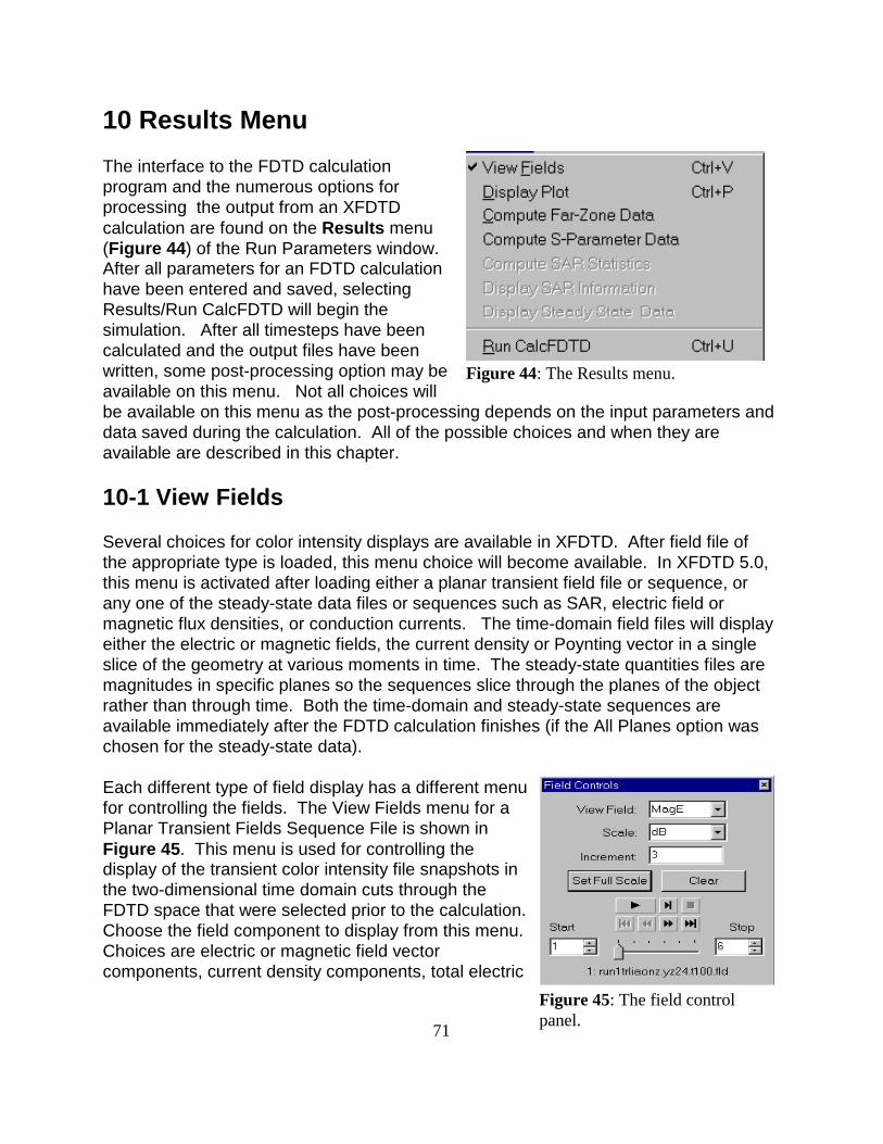
71

Figure 44: The Results menu.

Figure 45: The field controlpanel.

10 Results Menu

The interface to the FDTD calculationprogram and the numerous options forprocessing the output from an XFDTDcalculation are found on the Results menu (Figure 44) of the Run Parameters window. After all parameters for an FDTD calculationhave been entered and saved, selectingResults/Run CalcFDTD will begin thesimulation. After all timesteps have beencalculated and the output files have beenwritten, some post-processing option may beavailable on this menu. Not all choices willbe available on this menu as the post-processing depends on the input parameters anddata saved during the calculation. All of the possible choices and when they areavailable are described in this chapter.

10-1 View Fields

Several choices for color intensity displays are available in XFDTD. After field file ofthe appropriate type is loaded, this menu choice will become available. In XFDTD 5.0,this menu is activated after loading either a planar transient field file or sequence, orany one of the steady-state data files or sequences such as SAR, electric field ormagnetic flux densities, or conduction currents. The time-domain field files will displayeither the electric or magnetic fields, the current density or Poynting vector in a singleslice of the geometry at various moments in time. The steady-state quantities files aremagnitudes in specific planes so the sequences slice through the planes of the objectrather than through time. Both the time-domain and steady-state sequences areavailable immediately after the FDTD calculation finishes (if the All Planes option waschosen for the steady-state data).

Each different type of field display has a different menufor controlling the fields. The View Fields menu for aPlanar Transient Fields Sequence File is shown inFigure 45. This menu is used for controlling thedisplay of the transient color intensity file snapshots inthe two-dimensional time domain cuts through theFDTD space that were selected prior to the calculation. Choose the field component to display from this menu. Choices are electric or magnetic field vectorcomponents, current density components, total electric

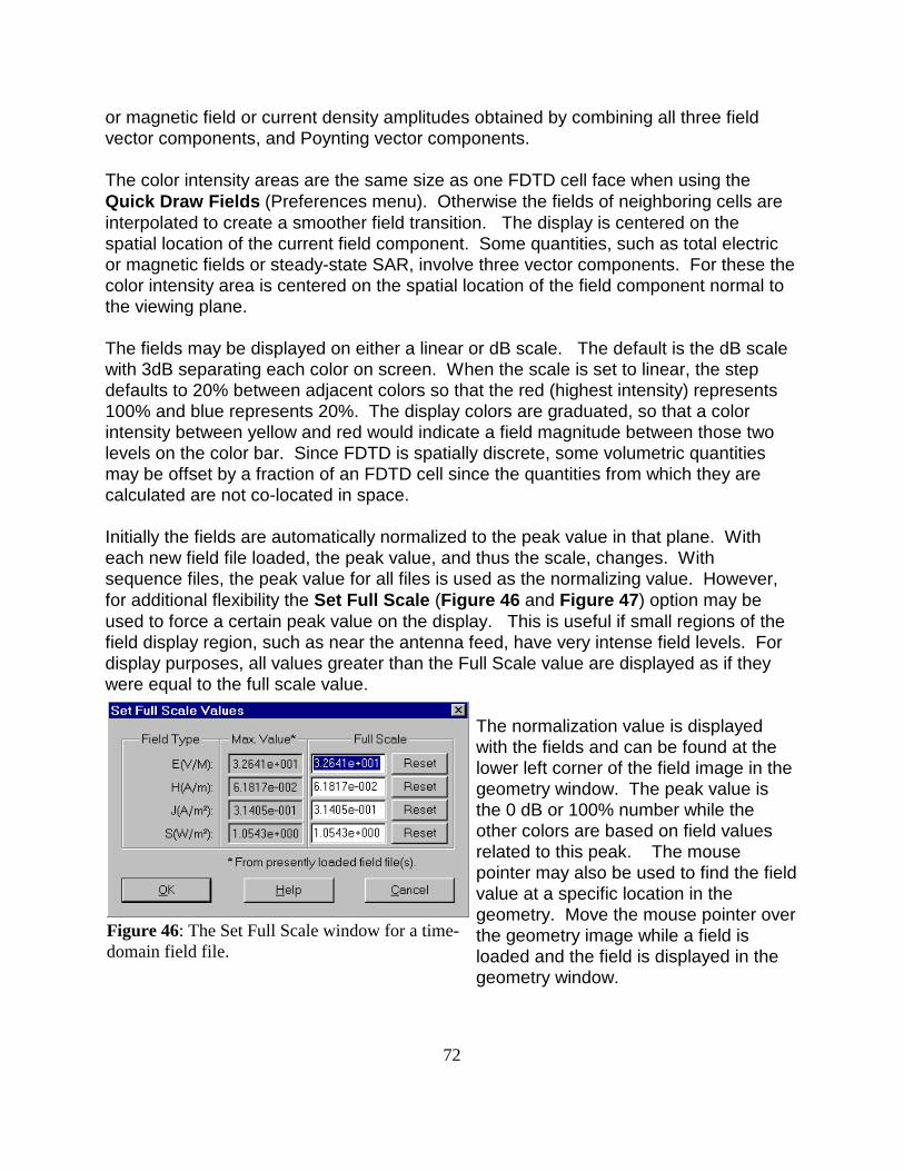
72

Figure 46: The Set Full Scale window for a time-domain field file.

or magnetic field or current density amplitudes obtained by combining all three fieldvector components, and Poynting vector components. The color intensity areas are the same size as one FDTD cell face when using theQuick Draw Fields (Preferences menu). Otherwise the fields of neighboring cells areinterpolated to create a smoother field transition. The display is centered on thespatial location of the current field component. Some quantities, such as total electricor magnetic fields or steady-state SAR, involve three vector components. For these thecolor intensity area is centered on the spatial location of the field component normal tothe viewing plane.

The fields may be displayed on either a linear or dB scale. The default is the dB scalewith 3dB separating each color on screen. When the scale is set to linear, the stepdefaults to 20% between adjacent colors so that the red (highest intensity) represents100% and blue represents 20%. The display colors are graduated, so that a colorintensity between yellow and red would indicate a field magnitude between those twolevels on the color bar. Since FDTD is spatially discrete, some volumetric quantitiesmay be offset by a fraction of an FDTD cell since the quantities from which they arecalculated are not co-located in space.

Initially the fields are automatically normalized to the peak value in that plane. Witheach new field file loaded, the peak value, and thus the scale, changes. Withsequence files, the peak value for all files is used as the normalizing value. However,for additional flexibility the Set Full Scale (Figure 46 and Figure 47) option may beused to force a certain peak value on the display. This is useful if small regions of thefield display region, such as near the antenna feed, have very intense field levels. Fordisplay purposes, all values greater than the Full Scale value are displayed as if theywere equal to the full scale value.

The normalization value is displayedwith the fields and can be found at thelower left corner of the field image in thegeometry window. The peak value isthe 0 dB or 100% number while theother colors are based on field valuesrelated to this peak. The mousepointer may also be used to find the fieldvalue at a specific location in thegeometry. Move the mouse pointer overthe geometry image while a field isloaded and the field is displayed in thegeometry window.

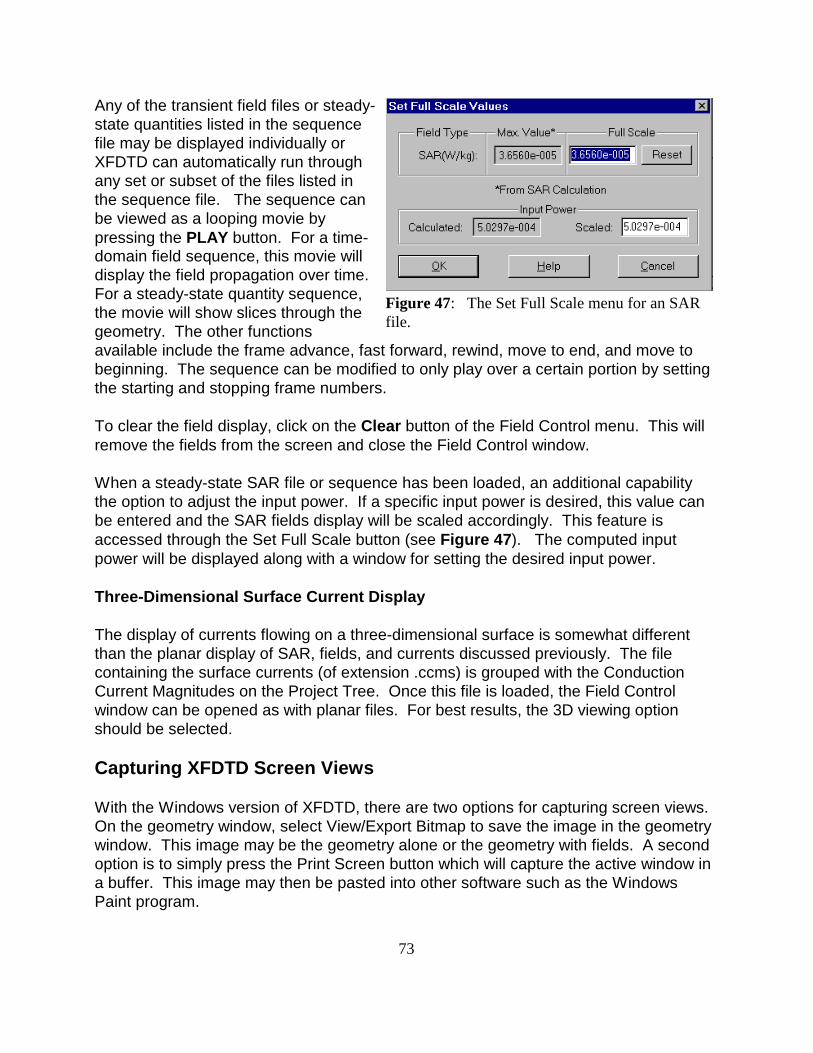
73

Figure 47: The Set Full Scale menu for an SARfile.

Any of the transient field files or steady-state quantities listed in the sequencefile may be displayed individually orXFDTD can automatically run throughany set or subset of the files listed inthe sequence file. The sequence canbe viewed as a looping movie bypressing the PLAY button. For a time-domain field sequence, this movie willdisplay the field propagation over time. For a steady-state quantity sequence,the movie will show slices through thegeometry. The other functionsavailable include the frame advance, fast forward, rewind, move to end, and move tobeginning. The sequence can be modified to only play over a certain portion by settingthe starting and stopping frame numbers.

To clear the field display, click on the Clear button of the Field Control menu. This willremove the fields from the screen and close the Field Control window.

When a steady-state SAR file or sequence has been loaded, an additional capabilitythe option to adjust the input power. If a specific input power is desired, this value canbe entered and the SAR fields display will be scaled accordingly. This feature isaccessed through the Set Full Scale button (see Figure 47). The computed inputpower will be displayed along with a window for setting the desired input power.

Three-Dimensional Surface Current Display

The display of currents flowing on a three-dimensional surface is somewhat differentthan the planar display of SAR, fields, and currents discussed previously. The filecontaining the surface currents (of extension .ccms) is grouped with the ConductionCurrent Magnitudes on the Project Tree. Once this file is loaded, the Field Controlwindow can be opened as with planar files. For best results, the 3D viewing optionshould be selected.

Capturing XFDTD Screen Views

With the Windows version of XFDTD, there are two options for capturing screen views. On the geometry window, select View/Export Bitmap to save the image in the geometrywindow. This image may be the geometry alone or the geometry with fields. A secondoption is to simply press the Print Screen button which will capture the active window ina buffer. This image may then be pasted into other software such as the WindowsPaint program.

74

In Unix XFDTD does not include the capability to provide users with digital files ofXFDTD displays directly. However, other software exists that can do this very well. To obtain digital images (.gif or .tif files or other formats) of any of the XFDTD screenimages we recommend the free software xv. It can be obtained over the Internet byanonymous FTP to ftp.cis.upenn.edu. The xv software is available from directorypub/xv. Executable versions of xv for many systems can be obtained using a webbrowser from www.trilon.com/xv/downloads.html#distributions. Additionally, the UnixXFDTD screen can be exported to a Windows machine using an X-server and imagesmay be saved using the Print Screen method described above.

10-2 Display Plot

Plots of most data saved by XFDTD can be displayed with the plotting tools includedwith the program. The plotting tool may be opened either through the Display PlotResults menu or from the icon on the button bar. The Display Plot window (shown inFigure 48 ) will then open and a plot of the desired data can be made and viewed.

There are three basic categories of plots in XFDTD, depending on the X-axis(abscissa) type. The first category is for time-domain plots which includes near-zonefield values, port/feed voltages and currents, and far-zone electric fields. The nextcategory is for plots versus frequency for data such as input impedance, S-parameters,gain or radar cross section (RCS), input/incident power, or port power. Finally, plotsversus angle may be viewed for gain or RCS patterns versus azimuth or elevation.

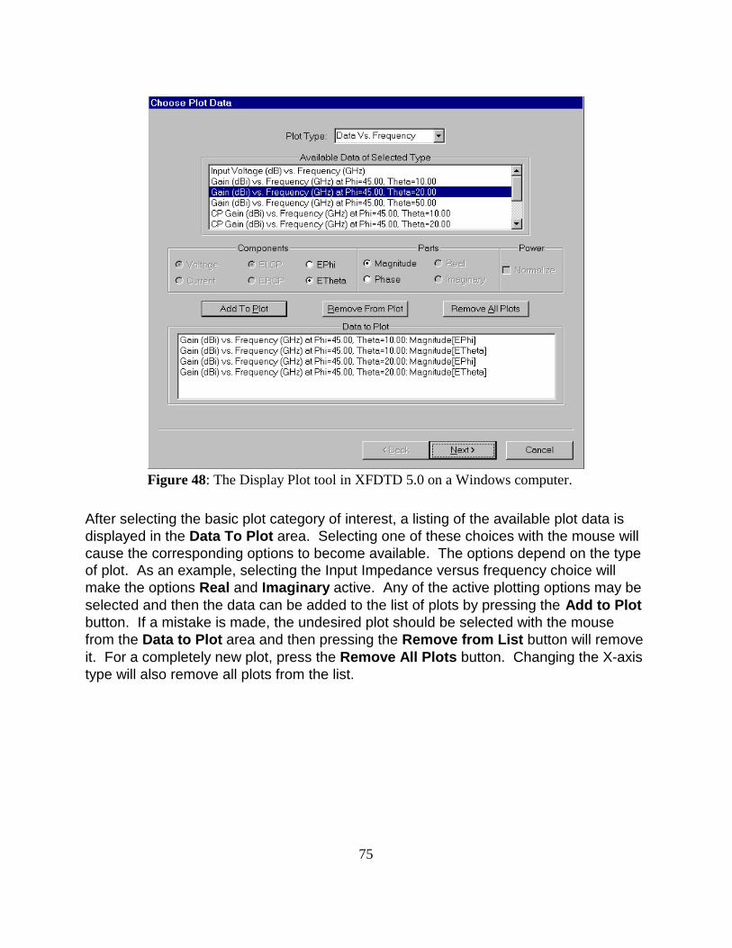
75

Figure 48: The Display Plot tool in XFDTD 5.0 on a Windows computer.

After selecting the basic plot category of interest, a listing of the available plot data isdisplayed in the Data To Plot area. Selecting one of these choices with the mouse willcause the corresponding options to become available. The options depend on the typeof plot. As an example, selecting the Input Impedance versus frequency choice willmake the options Real and Imaginary active. Any of the active plotting options may beselected and then the data can be added to the list of plots by pressing the Add to Plotbutton. If a mistake is made, the undesired plot should be selected with the mousefrom the Data to Plot area and then pressing the Remove from List button will removeit. For a completely new plot, press the Remove All Plots button. Changing the X-axistype will also remove all plots from the list.

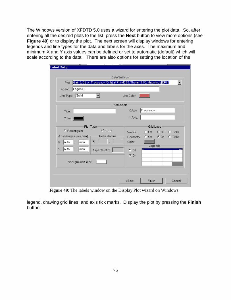
76

Figure 49: The labels window on the Display Plot wizard on Windows.

The Windows version of XFDTD 5.0 uses a wizard for entering the plot data. So, afterentering all the desired plots to the list, press the Next button to view more options (seeFigure 49) or to display the plot. The next screen will display windows for enteringlegends and line types for the data and labels for the axes. The maximum andminimum X and Y axis values can be defined or set to automatic (default) which willscale according to the data. There are also options for setting the location of the

legend, drawing grid lines, and axis tick marks. Display the plot by pressing the Finishbutton.

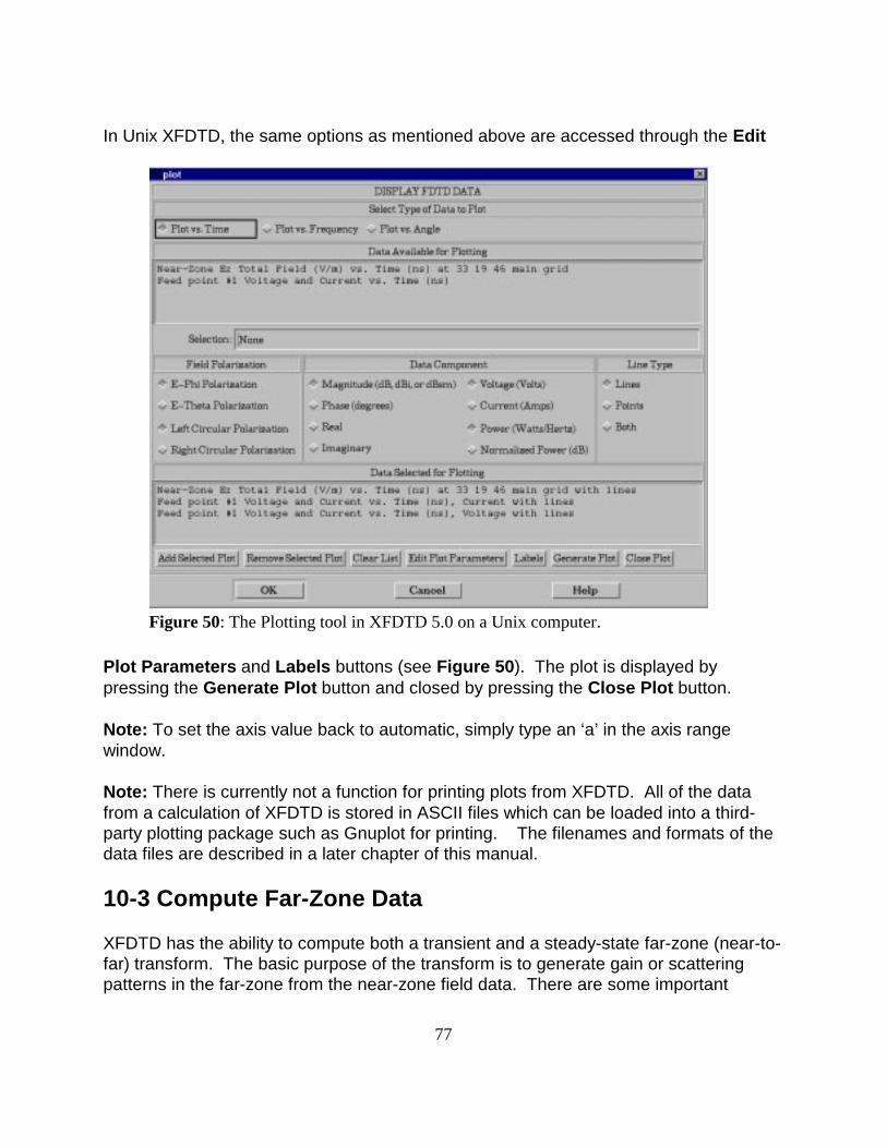
77

Figure 50: The Plotting tool in XFDTD 5.0 on a Unix computer.

In Unix XFDTD, the same options as mentioned above are accessed through the Edit

Plot Parameters and Labels buttons (see Figure 50). The plot is displayed bypressing the Generate Plot button and closed by pressing the Close Plot button.

Note: To set the axis value back to automatic, simply type an ‘a’ in the axis rangewindow.

Note: There is currently not a function for printing plots from XFDTD. All of the datafrom a calculation of XFDTD is stored in ASCII files which can be loaded into a third-party plotting package such as Gnuplot for printing. The filenames and formats of thedata files are described in a later chapter of this manual.

10-3 Compute Far-Zone Data

XFDTD has the ability to compute both a transient and a steady-state far-zone (near-to-far) transform. The basic purpose of the transform is to generate gain or scatteringpatterns in the far-zone from the near-zone field data. There are some important

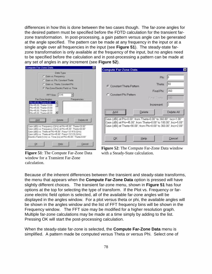
78

Figure 51: The Compute Far-Zone Datawindow for a Transient Far-Zonecalculation.

Figure 52: The Compute Far-Zone Data windowwith a Steady-State calculation.

differences in how this is done between the two cases though. The far-zone angles forthe desired pattern must be specified before the FDTD calculation for the transient far-zone transformation. In post-processing, a gain pattern versus angle can be generatedat the angle specified. The pattern can be made at any frequency in the input or at asingle angle over all frequencies in the input (see Figure 51). The steady-state far-zone transformation is only available at the frequency of the input, but no angles needto be specified before the calculation and in post-processing a pattern can be made atany set of angles in any increment (see Figure 52).

Because of the inherent differences between the transient and steady-state transforms,the menu that appears when the Compute Far-Zone Data option is pressed will haveslightly different choices. The transient far-zone menu, shown in Figure 51 has fouroptions at the top for selecting the type of transform. If the Plot vs. Frequency or far-zone electric field option is selected, all of the available far-zone angles will bedisplayed in the angles window. For a plot versus theta or phi, the available angles willbe shown in the angles window and the list of FFT frequency bins will be shown in theFrequency window. The FFT size may be modified for a higher resolution graph. Multiple far-zone calculations may be made at a time simply by adding to the list. Pressing OK will start the post-processing calculation.

When the steady-state far-zone is selected, the Compute Far-Zone Data menu issimplified. A pattern made be computed versus Theta or versus Phi. Select one of

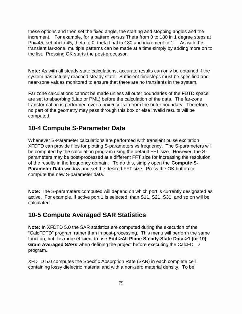
79

these options and then set the fixed angle, the starting and stopping angles and theincrement. For example, for a pattern versus Theta from 0 to 180 in 1 degree steps atPhi=45, set phi to 45, theta to 0, theta final to 180 and increment to 1. As with thetransient far-zone, multiple patterns can be made at a time simply by adding more on tothe list. Pressing OK starts the post-processor.

Note: As with all steady-state calculations, accurate results can only be obtained if thesystem has actually reached steady state. Sufficient timesteps must be specified andnear-zone values monitored to ensure that there are no transients in the system.

Far zone calculations cannot be made unless all outer boundaries of the FDTD spaceare set to absorbing (Liao or PML) before the calculation of the data. The far-zonetransformation is performed over a box 5 cells in from the outer boundary. Therefore,no part of the geometry may pass through this box or else invalid results will becomputed.

10-4 Compute S-Parameter Data

Whenever S-Parameter calculations are performed with transient pulse excitationXFDTD can provide files for plotting S-parameters vs frequency. The S-parameters willbe computed by the calculation program using the default FFT size. However, the S-parameters may be post-processed at a different FFT size for increasing the resolutionof the results in the frequency domain. To do this, simply open the Compute S-Parameter Data window and set the desired FFT size. Press the OK button tocompute the new S-parameter data.

Note: The S-parameters computed will depend on which port is currently designated asactive. For example, if active port 1 is selected, than S11, S21, S31, and so on will becalculated.

10-5 Compute Averaged SAR Statistics

Note: In XFDTD 5.0 the SAR statistics are computed during the execution of the“CalcFDTD” program rather than in post-processing. This menu will perform the samefunction, but it is more efficient to use Edit->All Plane Steady-State Data->1 (or 10)Gram Averaged SARs when defining the project before executing the CalcFDTDprogram.

XFDTD 5.0 computes the Specific Absorption Rate (SAR) in each complete cellcontaining lossy dielectric material and with a non-zero material density. To be

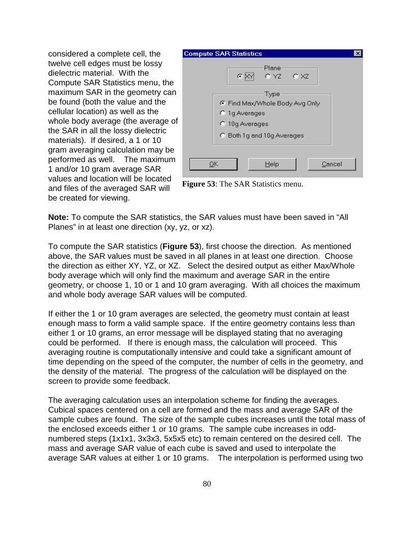
80

Figure 53: The SAR Statistics menu.

considered a complete cell, thetwelve cell edges must be lossydielectric material. With theCompute SAR Statistics menu, themaximum SAR in the geometry canbe found (both the value and thecellular location) as well as thewhole body average (the average ofthe SAR in all the lossy dielectricmaterials). If desired, a 1 or 10gram averaging calculation may beperformed as well. The maximum1 and/or 10 gram average SARvalues and location will be locatedand files of the averaged SAR willbe created for viewing.

Note: To compute the SAR statistics, the SAR values must have been saved in “AllPlanes” in at least one direction (xy, yz, or xz).

To compute the SAR statistics (Figure 53), first choose the direction. As mentionedabove, the SAR values must be saved in all planes in at least one direction. Choosethe direction as either XY, YZ, or XZ. Select the desired output as either Max/Wholebody average which will only find the maximum and average SAR in the entiregeometry, or choose 1, 10 or 1 and 10 gram averaging. With all choices the maximumand whole body average SAR values will be computed.

If either the 1 or 10 gram averages are selected, the geometry must contain at leastenough mass to form a valid sample space. If the entire geometry contains less thaneither 1 or 10 grams, an error message will be displayed stating that no averagingcould be performed. If there is enough mass, the calculation will proceed. Thisaveraging routine is computationally intensive and could take a significant amount oftime depending on the speed of the computer, the number of cells in the geometry, andthe density of the material. The progress of the calculation will be displayed on thescreen to provide some feedback.

The averaging calculation uses an interpolation scheme for finding the averages. Cubical spaces centered on a cell are formed and the mass and average SAR of thesample cubes are found. The size of the sample cubes increases until the total mass ofthe enclosed exceeds either 1 or 10 grams. The sample cube increases in odd-numbered steps (1x1x1, 3x3x3, 5x5x5 etc) to remain centered on the desired cell. Themass and average SAR value of each cube is saved and used to interpolate theaverage SAR values at either 1 or 10 grams. The interpolation is performed using two

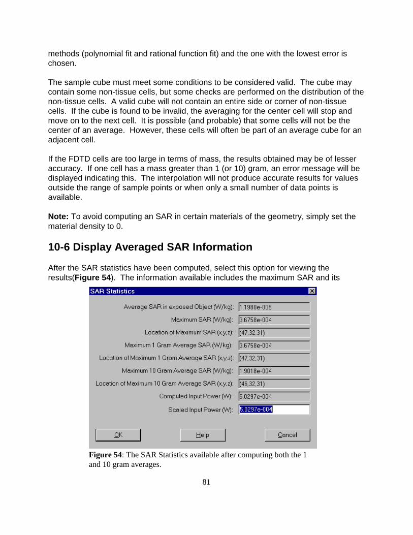
81

Figure 54: The SAR Statistics available after computing both the 1and 10 gram averages.

methods (polynomial fit and rational function fit) and the one with the lowest error ischosen.

The sample cube must meet some conditions to be considered valid. The cube maycontain some non-tissue cells, but some checks are performed on the distribution of thenon-tissue cells. A valid cube will not contain an entire side or corner of non-tissuecells. If the cube is found to be invalid, the averaging for the center cell will stop andmove on to the next cell. It is possible (and probable) that some cells will not be thecenter of an average. However, these cells will often be part of an average cube for anadjacent cell.

If the FDTD cells are too large in terms of mass, the results obtained may be of lesseraccuracy. If one cell has a mass greater than 1 (or 10) gram, an error message will bedisplayed indicating this. The interpolation will not produce accurate results for valuesoutside the range of sample points or when only a small number of data points isavailable.

Note: To avoid computing an SAR in certain materials of the geometry, simply set thematerial density to 0.

10-6 Display Averaged SAR Information

After the SAR statistics have been computed, select this option for viewing theresults(Figure 54). The information available includes the maximum SAR and its

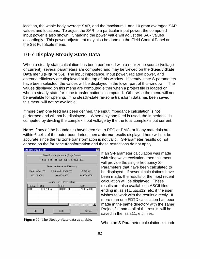
82

Figure 55: The Steady-State data available.

location, the whole body average SAR, and the maximum 1 and 10 gram averaged SARvalues and locations. To adjust the SAR to a particular input power, the computedinput power is also shown. Changing the power value will adjust the SAR valuesaccordingly. This power adjustment may also be done on the Field Control Panel onthe Set Full Scale menu.

10-7 Display Steady State Data

When a steady-state calculation has been performed with a near-zone source (voltageor current), several parameters are computed and may be viewed on the Steady StateData menu (Figure 55). The input impedance, input power, radiated power, andantenna efficiency are displayed at the top of this window. If steady-state S-parametershave been selected, the values will be displayed in the lower part of this window. Thevalues displayed on this menu are computed either when a project file is loaded orwhen a steady-state far-zone transformation is computed. Otherwise the menu will notbe available for opening. If no steady-state far-zone transform data has been saved,this menu will not be available.

If more than one feed has been defined, the input impedance calculation is notperformed and will not be displayed. When only one feed is used, the impedance iscomputed by dividing the complex input voltage by the the total complex input current.

Note: If any of the boundaries have been set to PEC or PMC, or if any materials arewithin 6 cells of the outer boundaries, then antenna results displayed here will not beaccurate since the far zone transformation is not valid. S-Parameter results do notdepend on the far zone transformation and these restrictions do not apply.

If an S-Parameter calculation was madewith sine wave excitation, then this menuwill provide the single frequency S-Parameters that have been calculated tobe displayed. If several calculations havebeen made, the results of the most recentcalculation will be displayed. Theseresults are also available in ASCII filesending in .ss.s11, .ss.s12, etc, if the userwishes to work with the results directly. Ifmore than one FDTD calculation has beenmade in the same directory with the sameProject file name all of the results will besaved in the .ss.s11, etc. files.

When an S-Parameter calculation is made

83

with the steady-state far zone transformation selected, then both the antenna data andthe S-Parameter data will be displayed. This may be useful, for example, when makingcalculations for a microstrip antenna when both S11 and input impedance are of interest.

84

11 User Generated Meshes

While XFDTD can be used interactively to generate complicated objects, in some casesit is preferable to generate the meshed geometry by some other means. This might beby writing special Fortran or C code to generate an object that can be described byequations, or it might be by translating an object described from another program into acubical mesh.

This process is described in [7]. A material type number must be associated with eachedge of the mesh. These material types correspond by number to those on the MaterialPalettes, so that "0" is free space, "1" is perfect conductor, "2-N" are dielectrics. InXFDTD 5.0, the maximum number for dielectrics is 27. If only dielectric materials arepresent only one set of edges need to be defined. If magnetic materials are present aseparate set of mesh edges must be defined. Once the mesh has been generated, itcan easily be put into a form that can be read by XFDTD.

Note: XFDTD expects the geometry file to have the extension .id

An example geometry file is shown in Table 1. The first line of a geometry file containsthe file version number. This indicates to XFDTD the format of the file and allows forbackward compatibility. The next line contains the variables which are the number ofcells in the FDTD space in the x, y, and z directions (NX, NY, NZ). This is followed bythree floating point variables giving the cell x, y, and z dimensions x, y, and z inmeters. In the example file shown, the space is 41 by 41 by 72 cells and each cell is a1 cm cube. The next line has three integer numbers, which are the offsets in cells of the geometry if it is to be used as a subgrid. For the example file these are all zero,since this file was meshed as a Main Grid and never used as a subgrid. The next linecontains a flag which indicates whether or not "fuzzy" cells are used in the mesh. Nofuzzy cells are used, and the value is zero.

The next part of the file is organized into 25 sets of 5 lines each, one set for each of the25 material types that can be defined. The labels start at Material 2 since Material type0 is reserved for free space, type 1 for perfect conductor. The first two lines of eachmaterial definition are used for labels and must contain the labels “emat02:” and“mmat02:” etc exactly as shown. The label, if defined, may be written after thedescriptor, but is best left blank at this point. The next line holds five floating pointnumbers for relative permittivity, conductivity (Siemens/meter), relative permeability,magnetic conductivity, and material density (kg/m3). The next line holds four floatingpoint numbers and one integer for defining the dispersive material parameters of staticrelative permittivity, relaxation time, resonant frequency, damping coefficient, and theinteger indicating the dispersive material type (0 for normal, 1 for Debye, 2 for Lorentz). The last line contains five floating point numbers and one integer for anisotropicmagnetic material parameters of Lamor Precession Frequency (rad/sec), saturation

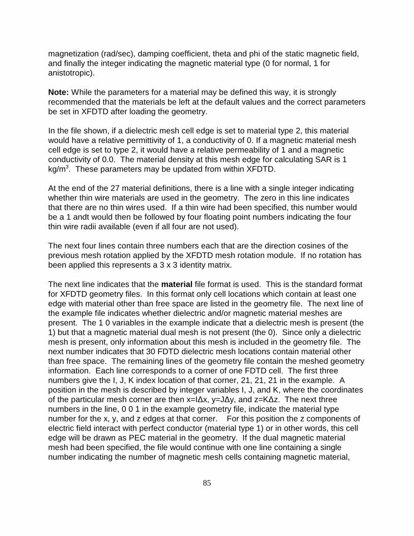
85

magnetization (rad/sec), damping coefficient, theta and phi of the static magnetic field,and finally the integer indicating the magnetic material type (0 for normal, 1 foranistotropic).

Note: While the parameters for a material may be defined this way, it is stronglyrecommended that the materials be left at the default values and the correct parametersbe set in XFDTD after loading the geometry.

In the file shown, if a dielectric mesh cell edge is set to material type 2, this materialwould have a relative permittivity of 1, a conductivity of 0. If a magnetic material meshcell edge is set to type 2, it would have a relative permeability of 1 and a magneticconductivity of 0.0. The material density at this mesh edge for calculating SAR is 1 kg/m3. These parameters may be updated from within XFDTD.

At the end of the 27 material definitions, there is a line with a single integer indicatingwhether thin wire materials are used in the geometry. The zero in this line indicatesthat there are no thin wires used. If a thin wire had been specified, this number wouldbe a 1 andt would then be followed by four floating point numbers indicating the fourthin wire radii available (even if all four are not used).

The next four lines contain three numbers each that are the direction cosines of theprevious mesh rotation applied by the XFDTD mesh rotation module. If no rotation hasbeen applied this represents a 3 x 3 identity matrix.

The next line indicates that the material file format is used. This is the standard formatfor XFDTD geometry files. In this format only cell locations which contain at least oneedge with material other than free space are listed in the geometry file. The next line ofthe example file indicates whether dielectric and/or magnetic material meshes arepresent. The 1 0 variables in the example indicate that a dielectric mesh is present (the1) but that a magnetic material dual mesh is not present (the 0). Since only a dielectricmesh is present, only information about this mesh is included in the geometry file. Thenext number indicates that 30 FDTD dielectric mesh locations contain material otherthan free space. The remaining lines of the geometry file contain the meshed geometryinformation. Each line corresponds to a corner of one FDTD cell. The first threenumbers give the I, J, K index location of that corner, 21, 21, 21 in the example. Aposition in the mesh is described by integer variables I, J, and K, where the coordinatesof the particular mesh corner are then x=I x, y=J y, and z=K z. The next threenumbers in the line, 0 0 1 in the example geometry file, indicate the material typenumber for the x, y, and z edges at that corner. For this position the z components ofelectric field interact with perfect conductor (material type 1) or in other words, this celledge will be drawn as PEC material in the geometry. If the dual magnetic materialmesh had been specified, the file would continue with one line containing a singlenumber indicating the number of magnetic mesh cells containing magnetic material,

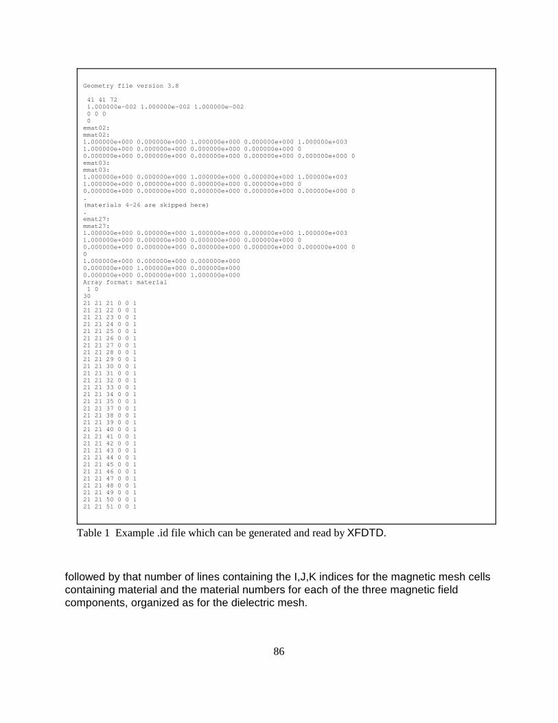
86

Geometry file version 3.8

41 41 72 1.000000e-002 1.000000e-002 1.000000e-002 0 0 0 0emat02: mmat02: 1.000000e+000 0.000000e+000 1.000000e+000 0.000000e+000 1.000000e+0031.000000e+000 0.000000e+000 0.000000e+000 0.000000e+000 00.000000e+000 0.000000e+000 0.000000e+000 0.000000e+000 0.000000e+000 0emat03: mmat03: 1.000000e+000 0.000000e+000 1.000000e+000 0.000000e+000 1.000000e+0031.000000e+000 0.000000e+000 0.000000e+000 0.000000e+000 00.000000e+000 0.000000e+000 0.000000e+000 0.000000e+000 0.000000e+000 0.(materials 4-26 are skipped here).emat27: mmat27: 1.000000e+000 0.000000e+000 1.000000e+000 0.000000e+000 1.000000e+0031.000000e+000 0.000000e+000 0.000000e+000 0.000000e+000 00.000000e+000 0.000000e+000 0.000000e+000 0.000000e+000 0.000000e+000 001.000000e+000 0.000000e+000 0.000000e+0000.000000e+000 1.000000e+000 0.000000e+0000.000000e+000 0.000000e+000 1.000000e+000Array format: material 1 03021 21 21 0 0 121 21 22 0 0 121 21 23 0 0 121 21 24 0 0 121 21 25 0 0 121 21 26 0 0 121 21 27 0 0 121 21 28 0 0 121 21 29 0 0 121 21 30 0 0 121 21 31 0 0 121 21 32 0 0 121 21 33 0 0 121 21 34 0 0 121 21 35 0 0 121 21 37 0 0 121 21 38 0 0 121 21 39 0 0 121 21 40 0 0 121 21 41 0 0 121 21 42 0 0 121 21 43 0 0 121 21 44 0 0 121 21 45 0 0 121 21 46 0 0 121 21 47 0 0 121 21 48 0 0 121 21 49 0 0 121 21 50 0 0 121 21 51 0 0 1

Table 1 Example .id file which can be generated and read by XFDTD.

followed by that number of lines containing the I,J,K indices for the magnetic mesh cellscontaining material and the material numbers for each of the three magnetic fieldcomponents, organized as for the dielectric mesh.

87

12 Subgrids

A very powerful feature of XFDTD is the ability to specify one or two subgrids withsmaller cells than the main grid. Proper use of this feature requires following severalrules. Improperly constructed subgrids can lead to instabilities, especially when manytimesteps are computed.

The subgrid implementation in XFDTD is extremely general. One important feature isthat perfect conductor and lossy dielectric materials can cross the subgrid-main gridboundaries. This allows a subgrid of finer resolution within a dielectric body. However,due to the interpolation of electromagnetic fields between main and subgrids, theremust be continuity of the materials in the normal direction to the boundary. Any non-free space materials must either continue through the boundary or be spaced at least 4cells away from the boundary for a 1/3 cell grid and 6 cells away from the boundary fora 1/5 cell grid. This spacing may need to be increased if stability problems occur or ifthe cell size is very small compared to the wavelength. This applies whether or not thematerial is passing through the main grid/subgrid boundary. Although sources may belocated within a subgrid, the source must be located away from the boundary of thesubgrid with the main grid by at least 4 cells (for 1/3 ratio) or 6 cells (for 1/5 ratio). Subgrid regions may not overlap, and must be separated by at least 3 main grid cells. A subgrid may not be located within 6 cells of the outer boundary.

The subgrid has the effect of overwriting any geometry in the main grid. If free spacecells in the subgrid overlap material in the main grid, the main grid materials will bechanged to free space during the calculation. There is no need to define the geometryin the main grid in the region of the subgrid, but if there is something there it will not bepart of the calculation. As an example, if there is a box in the main grid and anantenna will be added in a subgrid, any part of the box overlapped by the subgrid mustbe added to the subgrid geometry. Otherwise the overlapped box will be consideredfree space.

To further illustrate proper and improper subgrid techniques in XFDTD, some examplegeometries are shown here. First, if a dielectric material passes from the main gridinto the subgrid, there must not be discontinuities in the normal direction for the first fewcells of the subgrid. Also, the dielectric in the main grid must be reproduced in thesubgrid. See Figure 56 for an illustration. As is mentioned in the caption, the twodielectrics may be chosen as different XFDTD materials, but the constituitiveparameters must match.

A material in the subgrid may not end near the main grid-subgrid boundary as shown inFigure 57. This is an improperly formed subgrid which will possibly lead to an unstablecalculation.

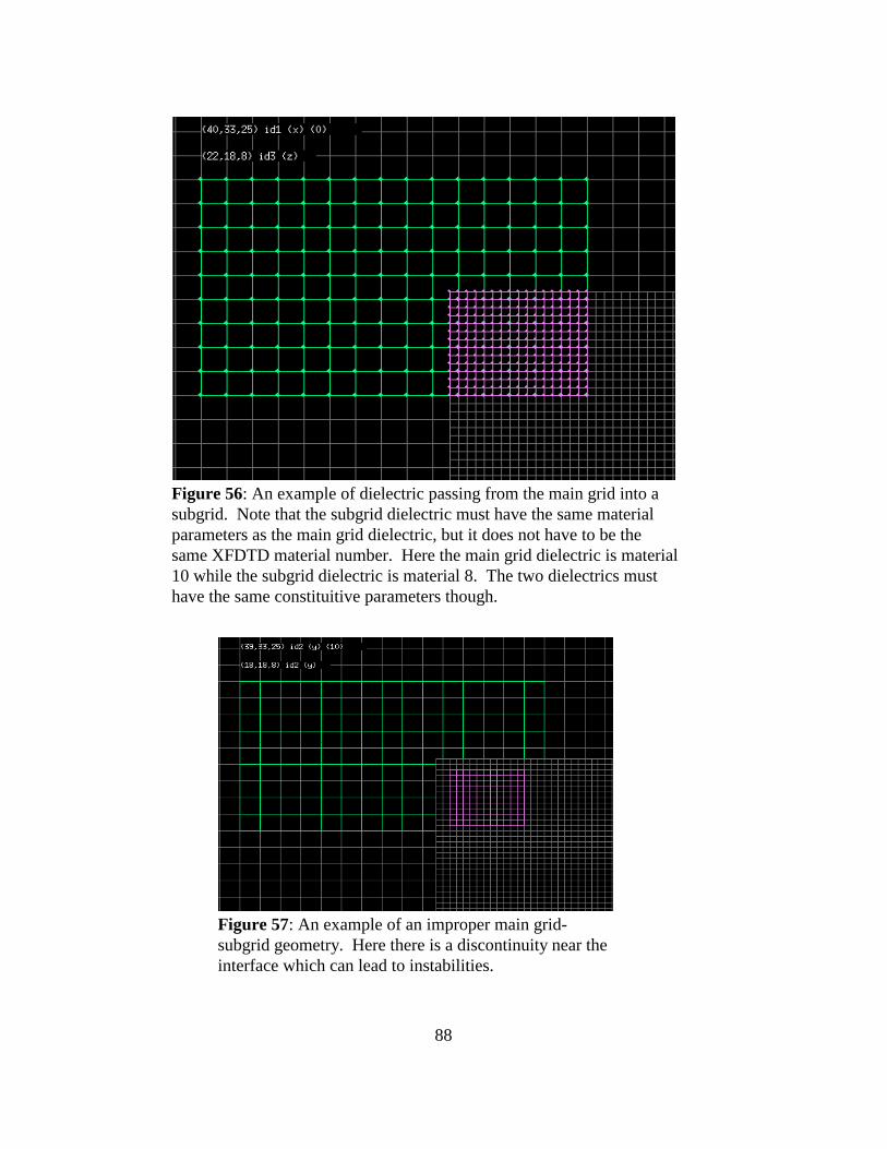
88

Figure 56: An example of dielectric passing from the main grid into asubgrid. Note that the subgrid dielectric must have the same materialparameters as the main grid dielectric, but it does not have to be thesame XFDTD material number. Here the main grid dielectric is material10 while the subgrid dielectric is material 8. The two dielectrics musthave the same constituitive parameters though.

Figure 57: An example of an improper main grid-subgrid geometry. Here there is a discontinuity near theinterface which can lead to instabilities.

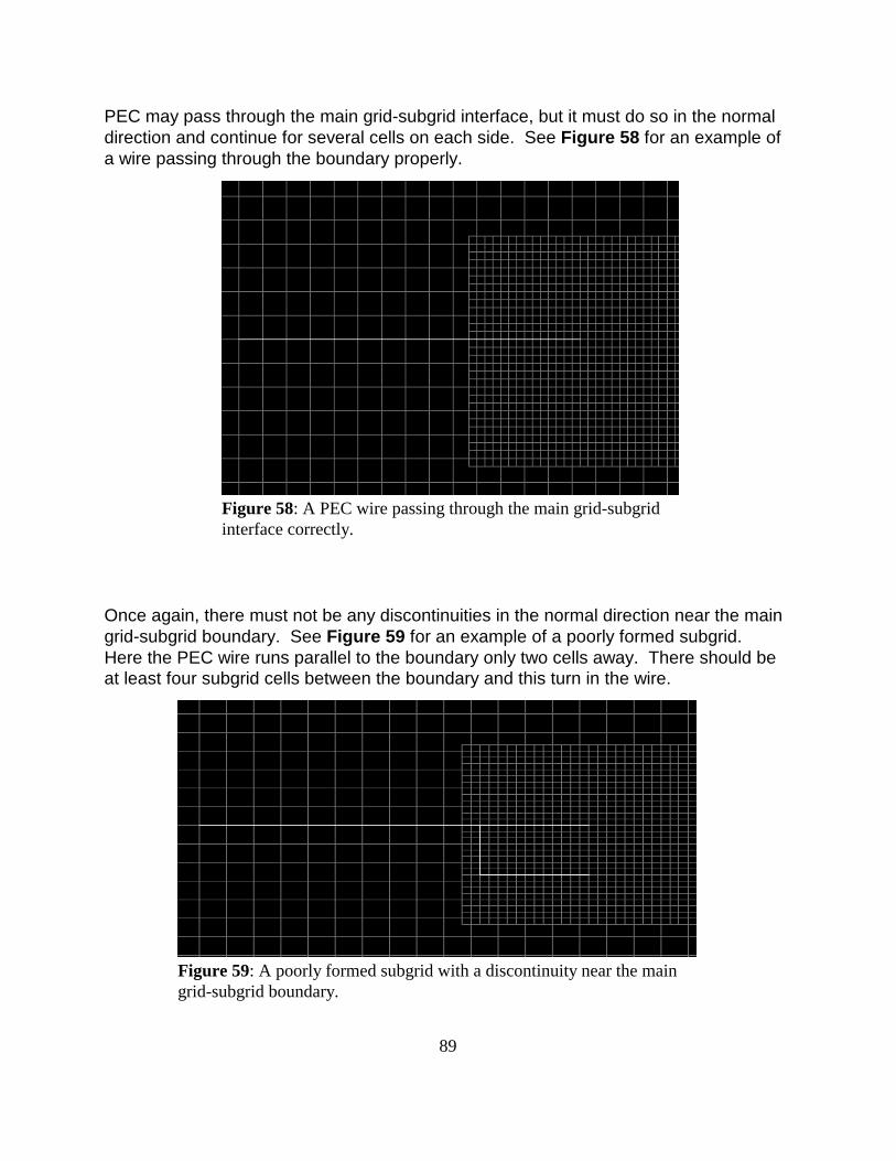
89

Figure 58: A PEC wire passing through the main grid-subgridinterface correctly.

Figure 59: A poorly formed subgrid with a discontinuity near the maingrid-subgrid boundary.

PEC may pass through the main grid-subgrid interface, but it must do so in the normaldirection and continue for several cells on each side. See Figure 58 for an example ofa wire passing through the boundary properly.

Once again, there must not be any discontinuities in the normal direction near the maingrid-subgrid boundary. See Figure 59 for an example of a poorly formed subgrid. Here the PEC wire runs parallel to the boundary only two cells away. There should beat least four subgrid cells between the boundary and this turn in the wire.

90

Note that the material types are specified independently in the main and subgrids. Thatis, material type 2 may be specified with different permittivity in the main and eachsubgrid. Material type 2 can even be a totally different type of material in each grid. For example, material type 2 could be a normal dielectric in the main grid, a Debyematerial in subgrid 1, and a Lorentz material in subgrid 2. When making FDTDcalculations the material inside the subgrid takes precedence over the materialsspecified in the same region of space in the main grid.

When materials cross the main grid/subgrid boundary, the alignment can be checkedby choosing to view All Grids. This is done by selecting the appropriate window in theWindows version of XFDTD, or through the View/Set Viewing Space menu in the Unixversion of XFDTD. If the Grid is displayed, then a slight overlap of the main andsubgrids is evident. This is due to the interpolation scheme used between the twogrids. For materials that cross the boundary, the same material type should be set inthe outer subgrid cells and the inner main grid cells that touch the main grid/subgridboundary. To help setting the alignment, the mouse cursor position for both grids isdisplayed when the view is set to All Grids. If material is to cross the boundary, theexact cellular coordinates of the material can be found in both grids.

The subgrid interpolation scheme is designed to allow dielectric materials to haveboundaries which cross the main grid-subgrid boundary. However, magnetic materials,if they cross the main grid-subgrid boundary, must be uniform within 5 cells of theboundary in order to avoid instability and inaccuracy.

The subgrid position within the main grid can be adjusted easily by changing the offsetof the subgrid. This is done by selecting the Subgrid Location in Main Grid optionfrom the Edit menu. The subgrid location is offset by slightly from what appears on thescreen due to some hidden cells in the subgrid. For example, setting the offset of a 3:1subgrid to 5 cells will start the subgrid just past cell 6. This is because there are two (or3 with 5:1 ratio) extra subgrid cells which are not drawn that are used as boundaries.

Computational Price for Subgrids: There is a computational price that must be paid in order to have the higher spatialresolution. A part of this price is additional memory requirements. For a 1/3 cell sizeratio, each main grid cell is replaced by 27 subgrid cells. For a 1/5 cell size ratio, eachmain grid cell is replaced by 125 subgrid cells. Even a fairly small subgrid region mayquickly need more memory than the entire main grid. So subgridding should be usedonly when absolutely needed.

Another computational burden imposed by subgrids is that, since the subgrid hassmaller cells, the time step in the subgrid is smaller than in the main grid. Furthermore,in order to increase stability, even the main grid time step is reduced below its normalvalue when subgrids are present. This is done automatically, but does mean that for

91

the same simulation time in seconds more FDTD time steps in the main grid arerequired.

While the XFDTD implementation of subgrids is designed to give greater freedom inapplication, the possibility of instability remains. This is due to the interpolation of thefields between the main and subgrids. When using subgrids, care should be takenwhen specifying the number of timesteps. The minimum number of time steps that willallow convergence to steady state or quiescent field values should be chosen. A subgrid must have dimensions that are at least four main grid cells as a minimum. Ifinstability is encountered, the symptom is rapidly growing field values that oscillaterapidly. If this happens, some possible ways to attempt to remove the instability are byspecifying fewer time steps, by changing to 1/3 size subgrid cells if 1/5 size cells havebeen specified, or by enlarging the subgrid size to allow a larger boundary between thegrids.

92

13 CALCFDTD Computer Program

The actual FDTD calculations are not made by the XFDTD graphical user interface. Once the geometry and project file are specified using the XFDTD menus, they must besaved before any calculation can be run. A separate computer program calledCalcFDTD makes the actual FDTD calculations. The XFDTD Graphical User Interfacethen will operate on and display the results of the FDTD calculations.

The CalcFDTD computer program reads the project and geometry files written byXFDTD and performs the actual FDTD calculations. It is an executable program written in the C language. It includes dynamic memory allocation so that different sizeFDTD spaces may be accommodated without allocating more computer memory thannecessary.

To run the CalcFDTD program, simply start it by selecting Run CalcFDTD from theResults menu. The progress of the calculation will be displayed in a window.

Additional options in Unix

In a Unix environment it is often more desirable to run CalcFDTD as a batch job or fromthe command line. To do so, simply enter the following:

calcfdtd50 [options] filename(.fdtd)

where "filename" is the name of the Project file (The .fdtd suffix need not included in thecalcfdtd50 command line).

For normal operation no options need be specified. There are several optionsavailable should they be of interest.

-rev print revision date

-ver print version number

-Z compress the field snapshot files (*.fld files) after creating them inorder to save disk space. XFDTD will read the compressed files

-gz gzip the field snapshot files (*.fld files) after creating them in orderto save disk space. For this function to be used the gzip andgunzip programs must be executable and in the path.

93

Figure 60: Creating the examplegeometry.

14 Example Procedures

In this section procedures for making an FDTD calculation will be illustrated by someexamples. Four cases are examined in detail. These are: a monopole on aconducting box, a microstrip meander line, a stripline Wilkinson power divider, and adipole near a lossy dielectric sphere. Several other examples are briefly discussed in aseparate section. The XFDTD files for the geometry and run parameters for allexamples are included with the XFDTD50 CDROM. The monopole on conducting boxexample is considered first and in some detail. New users are encouraged to followthis example before loading the provided files as it explains the basic operation ofXFDTD 5.0.

14-1 Monopole Antenna on a Conducting Box

This example was considered in [7] on pages 279-289. Here we will calculate theimpedance vs frequency for a 50 mm long monopole antenna on a 60 x 10 x 50 mmbox. The XFDTD50 input files monbox50.id and monbox50.fdtd furnished withXFDTD50 correspond to this example.

Following the description in [7] on page 283, we will use 1.67 mm cubical FDTD cells. This will give us 30 cells per wavelength at 6 GHz, which should provide very accurateresults. With this cell size the box will be 35 x 6 x 30 cells and the monopole will be 30cells long. With a 15 cell border our FDTD space will be 67 x 37 x 91 cells. For thecalculations in [7] a space of 130 x 90 x 180 cells was used, since the absorbing outerboundary used for those calculations required a much larger border in order to provideadequate absorption of the radiated fields. The savings for XFDTD are considerable. The calculation in [7] required over 2 million cells, while the calculation here needs justover 10% of that number.

1) After starting XFDTD by entering "xfdtd50" or launching from the Programs bar, clickon File then on New, or select the New Geometry icon from the Tool bar.

2) Choose to create a Main Grid. This will bring upthe menu shown in Figure 60. For our example weset the spatial increments as 1.67 millimeters, thespace dimensions as 67 x 37 x 91, and specify onlyan electric grid. Our example geometry has nomagnetic materials, so the magnetic grid is notneeded, nor will we need to create a Subgrid.

3) The next step is to put our geometry into theFDTD main grid. Open the Geometry Editing Toolsby selecting them from the Edit menu or by pressing the icon on the Tool bar. From the

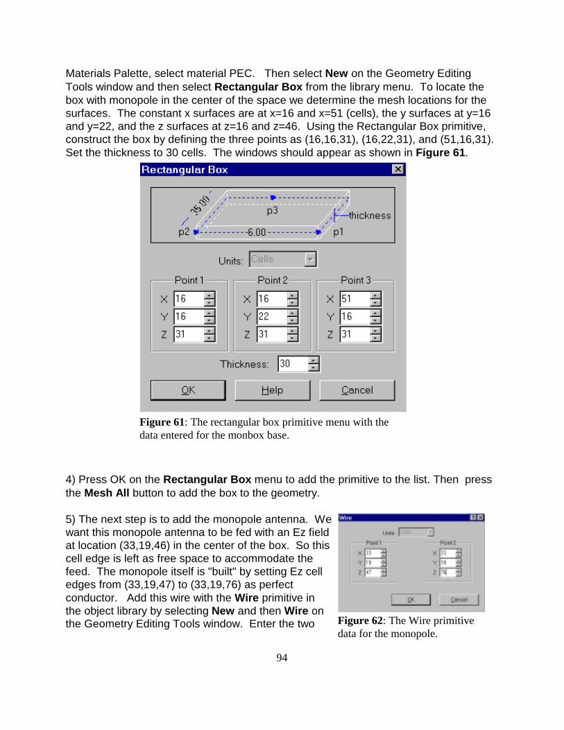
94

Figure 61: The rectangular box primitive menu with thedata entered for the monbox base.

Figure 62: The Wire primitivedata for the monopole.

Materials Palette, select material PEC. Then select New on the Geometry EditingTools window and then select Rectangular Box from the library menu. To locate thebox with monopole in the center of the space we determine the mesh locations for thesurfaces. The constant x surfaces are at x=16 and x=51 (cells), the y surfaces at y=16and y=22, and the z surfaces at z=16 and z=46. Using the Rectangular Box primitive,construct the box by defining the three points as (16,16,31), (16,22,31), and (51,16,31). Set the thickness to 30 cells. The windows should appear as shown in Figure 61.

4) Press OK on the Rectangular Box menu to add the primitive to the list. Then pressthe Mesh All button to add the box to the geometry.

5) The next step is to add the monopole antenna. Wewant this monopole antenna to be fed with an Ez fieldat location (33,19,46) in the center of the box. So thiscell edge is left as free space to accommodate thefeed. The monopole itself is "built" by setting Ez celledges from (33,19,47) to (33,19,76) as perfectconductor. Add this wire with the Wire primitive inthe object library by selecting New and then Wire onthe Geometry Editing Tools window. Enter the two

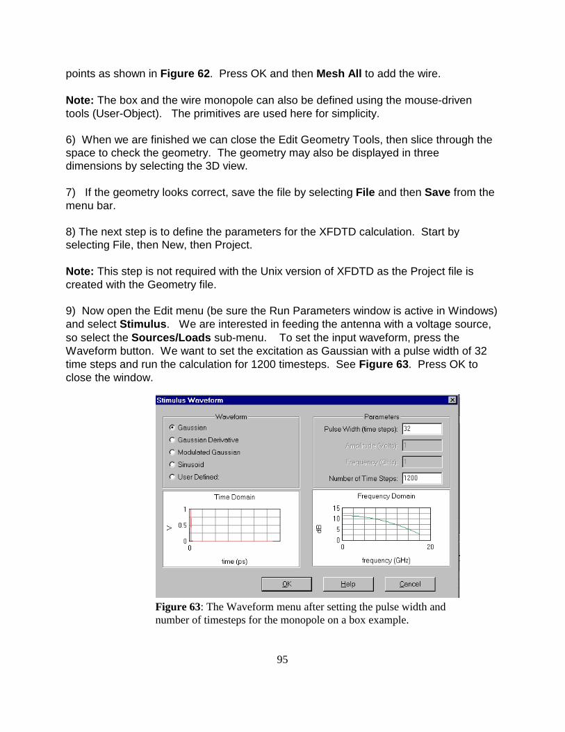
95

Figure 63: The Waveform menu after setting the pulse width andnumber of timesteps for the monopole on a box example.

points as shown in Figure 62. Press OK and then Mesh All to add the wire.

Note: The box and the wire monopole can also be defined using the mouse-driventools (User-Object). The primitives are used here for simplicity.

6) When we are finished we can close the Edit Geometry Tools, then slice through thespace to check the geometry. The geometry may also be displayed in threedimensions by selecting the 3D view.

7) If the geometry looks correct, save the file by selecting File and then Save from themenu bar.

8) The next step is to define the parameters for the XFDTD calculation. Start byselecting File, then New, then Project.

Note: This step is not required with the Unix version of XFDTD as the Project file iscreated with the Geometry file.

9) Now open the Edit menu (be sure the Run Parameters window is active in Windows) and select Stimulus. We are interested in feeding the antenna with a voltage source,so select the Sources/Loads sub-menu. To set the input waveform, press theWaveform button. We want to set the excitation as Gaussian with a pulse width of 32time steps and run the calculation for 1200 timesteps. See Figure 63. Press OK toclose the window.

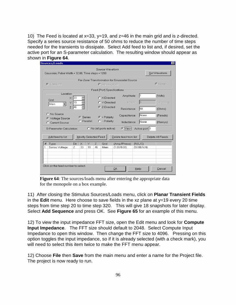
96

Figure 64: The sources/loads menu after entering the appropriate datafor the monopole on a box example.

10) The Feed is located at x=33, y=19, and z=46 in the main grid and is z-directed. Specify a series source resistance of 50 ohms to reduce the number of time stepsneeded for the transients to dissipate. Select Add feed to list and, if desired, set theactive port for an S-parameter calculation. The resulting window should appear asshown in Figure 64.

11) After closing the Stimulus Sources/Loads menu, click on Planar Transient Fieldsin the Edit menu. Here choose to save fields in the xz plane at y=19 every 20 timesteps from time step 20 to time step 320. This will give 18 snapshots for later display. Select Add Sequence and press OK. See Figure 65 for an example of this menu.

12) To view the input impedance FFT size, open the Edit menu and look for ComputeInput Impedance. The FFT size should default to 2048. Select Compute InputImpedance to open this window. Then change the FFT size to 4096. Pressing on thisoption toggles the input impedance, so if it is already selected (with a check mark), youwill need to select this item twice to make the FFT menu appear.

12) Choose File then Save from the main menu and enter a name for the Project file. The project is now ready to run.

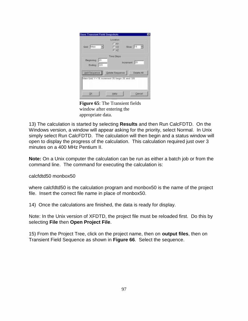
97

Figure 65: The Transient fieldswindow after entering theappropriate data.

13) The calculation is started by selecting Results and then Run CalcFDTD. On theWindows version, a window will appear asking for the priority, select Normal. In Unixsimply select Run CalcFDTD. The calculation will then begin and a status window willopen to display the progress of the calculation. This calculation required just over 3minutes on a 400 MHz Pentium II.

Note: On a Unix computer the calculation can be run as either a batch job or from thecommand line. The command for executing the calculation is:

calcfdtd50 monbox50

where calcfdtd50 is the calculation program and monbox50 is the name of the projectfile. Insert the correct file name in place of monbox50.

14) Once the calculations are finished, the data is ready for display.

Note: In the Unix version of XFDTD, the project file must be reloaded first. Do this byselecting File then Open Project File.

15) From the Project Tree, click on the project name, then on output files, then onTransient Field Sequence as shown in Figure 66. Select the sequence.

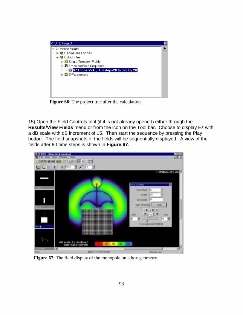
98

Figure 66: The project tree after the calculation.

Figure 67: The field display of the monopole on a box geometry.

15) Open the Field Controls tool (if it is not already opened) either through theResults/View Fields menu or from the icon on the Tool bar. Choose to display Ez witha dB scale with dB increment of 15. Then start the sequence by pressing the Playbutton. The field snapshots of the fields will be sequentially displayed. A view of thefields after 80 time steps is shown in Figure 67.

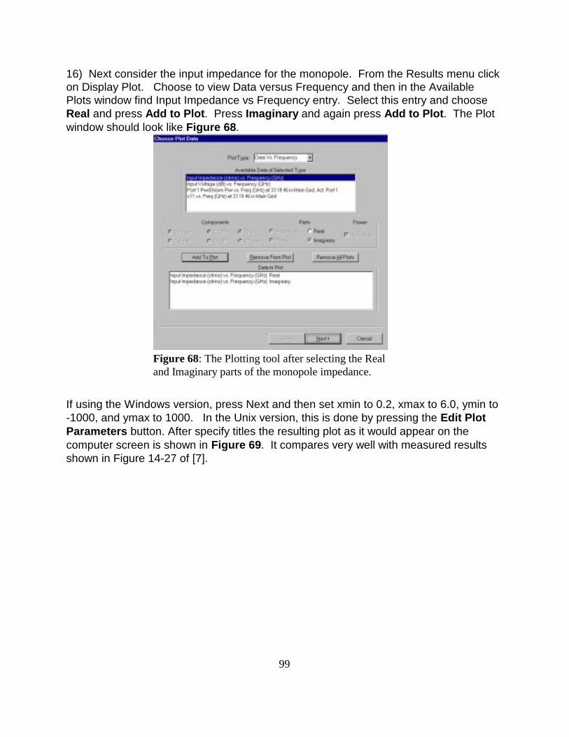
99

Figure 68: The Plotting tool after selecting the Realand Imaginary parts of the monopole impedance.

16) Next consider the input impedance for the monopole. From the Results menu clickon Display Plot. Choose to view Data versus Frequency and then in the AvailablePlots window find Input Impedance vs Frequency entry. Select this entry and chooseReal and press Add to Plot. Press Imaginary and again press Add to Plot. The Plotwindow should look like Figure 68.

If using the Windows version, press Next and then set xmin to 0.2, xmax to 6.0, ymin to-1000, and ymax to 1000. In the Unix version, this is done by pressing the Edit PlotParameters button. After specify titles the resulting plot as it would appear on thecomputer screen is shown in Figure 69. It compares very well with measured resultsshown in Figure 14-27 of [7].

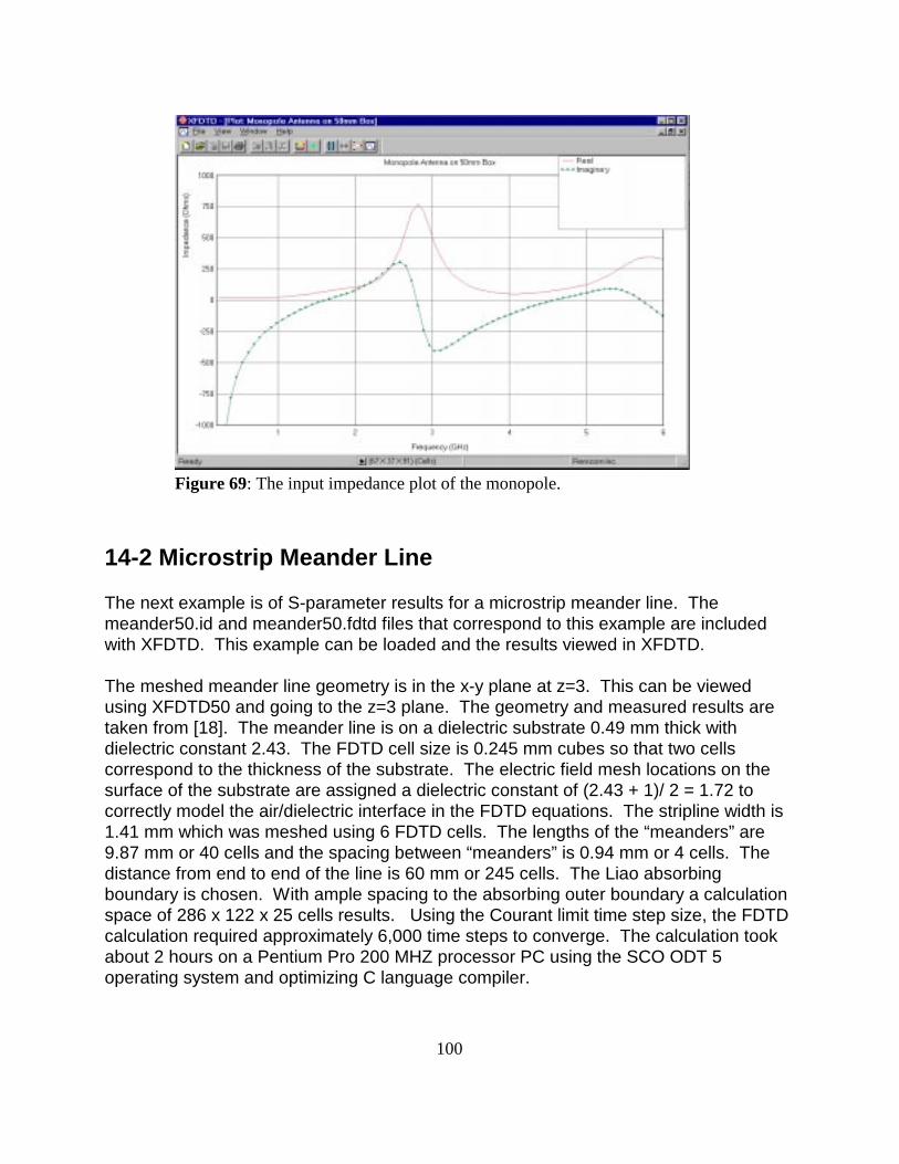
100

Figure 69: The input impedance plot of the monopole.

14-2 Microstrip Meander Line

The next example is of S-parameter results for a microstrip meander line. Themeander50.id and meander50.fdtd files that correspond to this example are includedwith XFDTD. This example can be loaded and the results viewed in XFDTD.

The meshed meander line geometry is in the x-y plane at z=3. This can be viewedusing XFDTD50 and going to the z=3 plane. The geometry and measured results aretaken from [18]. The meander line is on a dielectric substrate 0.49 mm thick withdielectric constant 2.43. The FDTD cell size is 0.245 mm cubes so that two cellscorrespond to the thickness of the substrate. The electric field mesh locations on thesurface of the substrate are assigned a dielectric constant of (2.43 + 1)/ 2 = 1.72 tocorrectly model the air/dielectric interface in the FDTD equations. The stripline width is1.41 mm which was meshed using 6 FDTD cells. The lengths of the “meanders” are9.87 mm or 40 cells and the spacing between “meanders” is 0.94 mm or 4 cells. Thedistance from end to end of the line is 60 mm or 245 cells. The Liao absorbingboundary is chosen. With ample spacing to the absorbing outer boundary a calculationspace of 286 x 122 x 25 cells results. Using the Courant limit time step size, the FDTDcalculation required approximately 6,000 time steps to converge. The calculation tookabout 2 hours on a Pentium Pro 200 MHZ processor PC using the SCO ODT 5operating system and optimizing C language compiler.

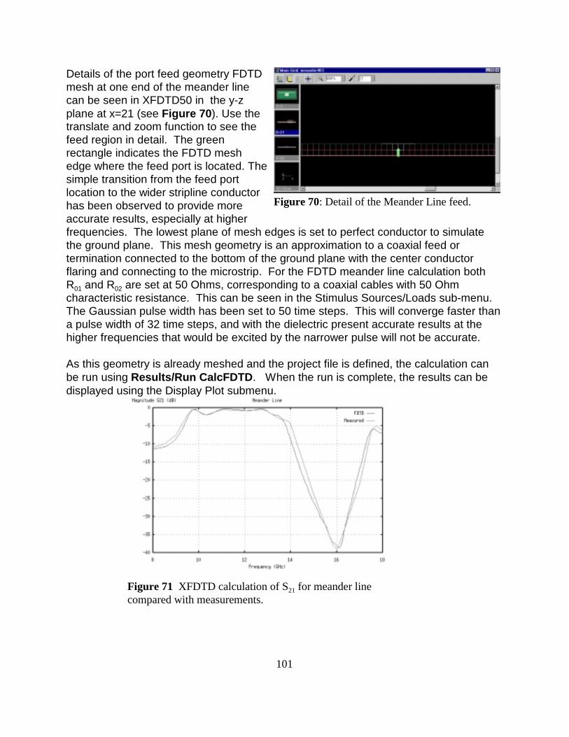
101

Figure 71 XFDTD calculation of S21 for meander linecompared with measurements.

Figure 70: Detail of the Meander Line feed.

Details of the port feed geometry FDTDmesh at one end of the meander linecan be seen in XFDTD50 in the y-zplane at x=21 (see Figure 70). Use thetranslate and zoom function to see thefeed region in detail. The greenrectangle indicates the FDTD meshedge where the feed port is located. Thesimple transition from the feed portlocation to the wider stripline conductorhas been observed to provide moreaccurate results, especially at higherfrequencies. The lowest plane of mesh edges is set to perfect conductor to simulatethe ground plane. This mesh geometry is an approximation to a coaxial feed ortermination connected to the bottom of the ground plane with the center conductorflaring and connecting to the microstrip. For the FDTD meander line calculation bothR01 and R02 are set at 50 Ohms, corresponding to a coaxial cables with 50 Ohmcharacteristic resistance. This can be seen in the Stimulus Sources/Loads sub-menu. The Gaussian pulse width has been set to 50 time steps. This will converge faster thana pulse width of 32 time steps, and with the dielectric present accurate results at thehigher frequencies that would be excited by the narrower pulse will not be accurate.

As this geometry is already meshed and the project file is defined, the calculation canbe run using Results/Run CalcFDTD. When the run is complete, the results can bedisplayed using the Display Plot submenu.

102

The result S21 is plotted in Figure 71 and compared with measurements from [18]. Theagreement is quite good, comparable or better than the calculated results given in [18]and much better than the Touchstone results also shown in [18].

14-3 Stripline Wilkinson Power Divider

This example is for a stripline Wilkinson power divider. The wilk50.id and wilk50.fdtdfiles that correspond to this example are included with XFDTD50. You are encouragedto load these files into XFDTD50 and follow along with the following discussion.

The layout of the power divider will be shown in XFDTD50 in the x-y plane at z=7. Port1 is at the bottom, Port 2 at the upper left, and Port 3 at the upper right. The FDTD cellsize is .112 x .112 x .127 mm, with the total FDTD space being 155 x 199 x 12 cells. The overall dimensions of the stripline conductors are 19.94 mm or 178 cells from Port2 to Port 3, and the overall distance from Port 1 to the far edge of conductor is 15.57mm or 139 cells. The dielectric has permittivity 2.94 and the total dielectric thickness is1.524 mm, with the stripline conductor sandwiched in the middle. The blue square is a100 Ohm isolation resistor fabricated using 100 Ohm/square resistive material.

Care must be taken in meshing the power divider. First the stripline planes of theFDTD space are set to conductor, while the 4 sides are terminated in Liao absorbingboundaries. The entire FDTD space is filled with dielectric except for the striplineconductor and the isolation resistor. The stripline conductor is meshed as one planethick perfect conductor. The isolation resistor is meshed using one plane thick lossydielectric with permittivity of free space and conductivity of 78.74 Ohms. This isobtained using a simple sheet impedance model [1] as the reciprocal of the product ofthe sheet resistance and the cell thickness. The cell thickness is set at 0.127 mm inthis dimension so that 12 cells correspond exactly to the dielectric thickness. The othertwo cell dimensions in the plane of the conductor were chosen to allow precisealignment of the mesh edges with the conductor steps.

A very important consideration is location of the mesh edges where the port sourcesand terminations are to be located. One approach might be to terminate the sideboundaries of the FDTD mesh normal to the stripline conductor with perfect conductorplanes. Then a mesh edge normal to the outer conductor plane could be used as thesource location, with the stripline conductor touching it and starting one cell inside themesh. This would correspond physically to a stripline constructed inside a metal boxwith all sides closed and fed by coaxial cables with the outer conductor attached to themetal box and the center conductor going through the metal box surface to feed thestripline.

This feed geometry, while a reasonable approximation to a realistic stripline circuit,

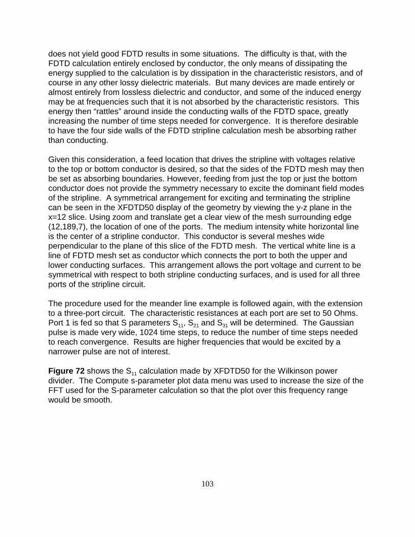
103

does not yield good FDTD results in some situations. The difficulty is that, with theFDTD calculation entirely enclosed by conductor, the only means of dissipating theenergy supplied to the calculation is by dissipation in the characteristic resistors, and ofcourse in any other lossy dielectric materials. But many devices are made entirely oralmost entirely from lossless dielectric and conductor, and some of the induced energymay be at frequencies such that it is not absorbed by the characteristic resistors. Thisenergy then “rattles” around inside the conducting walls of the FDTD space, greatlyincreasing the number of time steps needed for convergence. It is therefore desirableto have the four side walls of the FDTD stripline calculation mesh be absorbing ratherthan conducting.

Given this consideration, a feed location that drives the stripline with voltages relativeto the top or bottom conductor is desired, so that the sides of the FDTD mesh may thenbe set as absorbing boundaries. However, feeding from just the top or just the bottomconductor does not provide the symmetry necessary to excite the dominant field modesof the stripline. A symmetrical arrangement for exciting and terminating the striplinecan be seen in the XFDTD50 display of the geometry by viewing the y-z plane in thex=12 slice. Using zoom and translate get a clear view of the mesh surrounding edge(12,189,7), the location of one of the ports. The medium intensity white horizontal lineis the center of a stripline conductor. This conductor is several meshes wideperpendicular to the plane of this slice of the FDTD mesh. The vertical white line is aline of FDTD mesh set as conductor which connects the port to both the upper andlower conducting surfaces. This arrangement allows the port voltage and current to besymmetrical with respect to both stripline conducting surfaces, and is used for all threeports of the stripline circuit.

The procedure used for the meander line example is followed again, with the extensionto a three-port circuit. The characteristic resistances at each port are set to 50 Ohms. Port 1 is fed so that S parameters S11, S21 and S31 will be determined. The Gaussianpulse is made very wide, 1024 time steps, to reduce the number of time steps neededto reach convergence. Results are higher frequencies that would be excited by anarrower pulse are not of interest.

Figure 72 shows the S11 calculation made by XFDTD50 for the Wilkinson powerdivider. The Compute s-parameter plot data menu was used to increase the size of theFFT used for the S-parameter calculation so that the plot over this frequency rangewould be smooth.

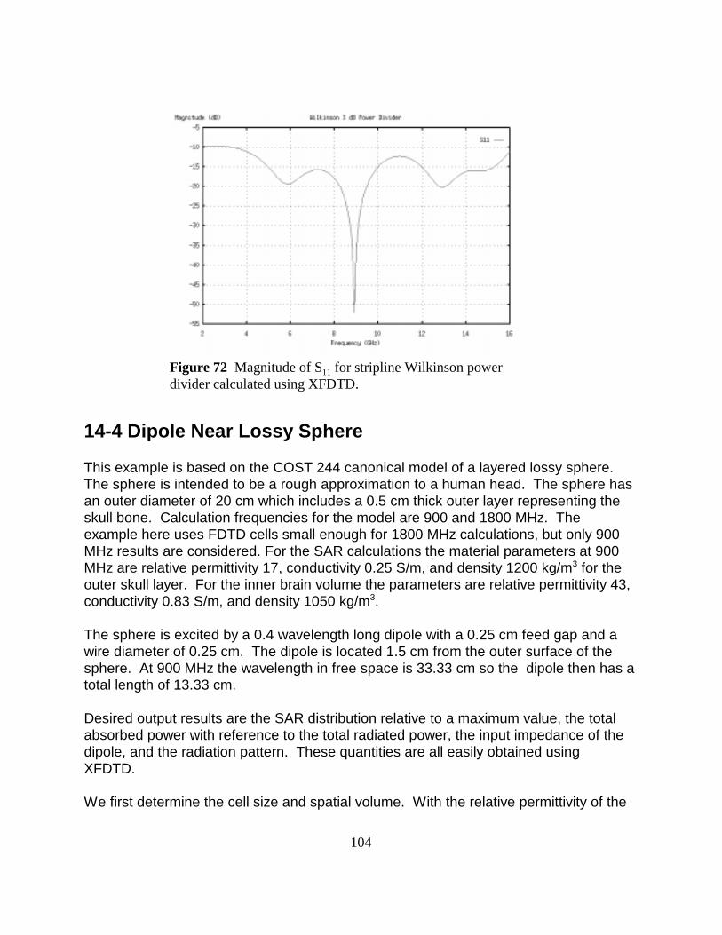
104

Figure 72 Magnitude of S11 for stripline Wilkinson powerdivider calculated using XFDTD.

14-4 Dipole Near Lossy Sphere This example is based on the COST 244 canonical model of a layered lossy sphere. The sphere is intended to be a rough approximation to a human head. The sphere hasan outer diameter of 20 cm which includes a 0.5 cm thick outer layer representing theskull bone. Calculation frequencies for the model are 900 and 1800 MHz. Theexample here uses FDTD cells small enough for 1800 MHz calculations, but only 900MHz results are considered. For the SAR calculations the material parameters at 900MHz are relative permittivity 17, conductivity 0.25 S/m, and density 1200 kg/m3 for theouter skull layer. For the inner brain volume the parameters are relative permittivity 43,conductivity 0.83 S/m, and density 1050 kg/m3.

The sphere is excited by a 0.4 wavelength long dipole with a 0.25 cm feed gap and awire diameter of 0.25 cm. The dipole is located 1.5 cm from the outer surface of thesphere. At 900 MHz the wavelength in free space is 33.33 cm so the dipole then has atotal length of 13.33 cm.

Desired output results are the SAR distribution relative to a maximum value, the totalabsorbed power with reference to the total radiated power, the input impedance of thedipole, and the radiation pattern. These quantities are all easily obtained usingXFDTD.

We first determine the cell size and spatial volume. With the relative permittivity of the

105

brain tissue of 43, the shortest wavelength in the problem space is inside the brain, andis the 1800 MHz free space wavelength divided by the square root of 43, orapproximately 0.25 cm. This is also a convenient cell size for modeling the dipole gapand wire diameter, since the wire diameter is approximately the cell size. We could usethe XFDTD capability to include thin wires, but for this cell size and wire diameter it isnot needed. This cell size will provide 20 cells per wavelength at 900 MHz. This ismore than needed, but lets us use the same mesh for both frequencies.

With 0.25 cm FDTD cells, the sphere diameter is 80 cells and the dipole is 6 cells awayfrom the sphere surface. With a 20 cell free space border on all sides, this results in a130 x 120 x 120 cell space where we have allowed a few extra cells to separate thedipole from the outer boundary.

To set up the calculation start XFDTD and create a space 130 x 120 x 120 cells with0.25 cm cells. From the Geometry Editing Tools window, choose the sphere. One wayto mesh the two layers is to first mesh a 40 cell radius sphere centered at 60, 60, 60with material type 3. Then mesh a 38 cell sphere centered at the same location withmaterial type 2. The two cell layers corresponds to the 0.5 cm skull outer layer. Meshing the larger sphere first assures that there will be no air gaps where the layersjoin.

Next mesh the dipole. This could be done manually with the mouse, but can also bedone with the wire function from the library. The dipole is 53 cells long, so each dipolearm is 26 cells and there is a 1 cell gap at the center. We choose to put the dipole inthe xz plane at y=60. The x location of the wire is 46 cells from the center of thesphere, or x=106. The center of the dipole will be cell edge 106, 60, 60. To use thewire library function for the upper half of the dipole wire, set end 1 to 106, 60, 61 andend 2 to 106, 60, 87 with material PEC then click on add object. If the XFDTD slice isset to xz plane at y=60 the upper half of the dipole should appear. To mesh the lowerhalf, set end 1 in the wire function to 106, 60, 60 and end 2 to 106, 60, 34. The resultshould be the wire dipole with each arm 26 cells and a 1 cell gap in the middle.

Be sure to set the relative permittivity and conductivity of materials 2 and 3 to theparameters given above for brain and skull. Also set the densities for materials 2 and 3to the brain and skull parameters given above.

Next set the excitation of the calculation. From the Stimulus-Sources/Loads menu adda +Z voltage source at location 106, 60, 60 with a zero resistance source resistor. Thenset the frequency to 900 MHz (0.9 GHz) with 2500 time steps. Choose the steadystate far zone transformation so far zone patterns can be calculated.

Finally save the necessary results. Using the Save Near Zone Data menu save the Ezand Jz electric field and current density at the feed location, 106, 60, 60. In order to

106

calculate the maximum SAR, from the FDTD-Save All Steady State Quantities-SARPlanes menu save all SAR xz planes.

Then save the geometry and XFDTD project files using the appropriate menus fromFile. Then run the calculation. This calculation took approximately 55 minutes on a400 MHz Pentium II computer.

Once the calculations are finished reload the project file to perform somepostprocessing. From the Results-Steady State Data display you should see the feedpoint 1 impedance of 27.90-j111.82 ohms. The antenna efficiency is 29%. This meansthat 71% of the power supplied to the antenna is absorbed in the lossy sphere.

In order to obtain SAR information, use the Results-Compute SAR Statistics menu andselect the x-z plane since these were the planes saved. Once the SAR calculation iscomplete, you can then use the Results-Display SAR Information menu to see theresulting SAR information. The input power can be scaled on this menu. With thescale input power set to 1 Watt on this menu, the Maximum SAR is approximately 11.4W/kg.

The SAR distribution can be seen in false color using XFDTD. To do this load a SARfile using the Project Tree. The distribution for the unaveraged SAR in the y=60 planeis shown in Figure 73. To allow the colors to be displayed more clearly the materialdisplay is toggled off. The dipole is actually in this plane, and will be visible when thefile is first loaded. The color display may also be changed by changing the dBincrement from the 18 dB used for this figure.

The far zone radiation pattern can be obtained from the Results-Compute Far ZonePlot Data. Choose a constant theta pattern with theta = 90 degrees, and let phi coverfrom 0 to 360 degrees in 2 degree increments. The pattern calculation will requiresome time. Once it is complete the result can be displayed using the Results-DisplayPlot menu. The result for E-theta polarization is shown in Figure 74.

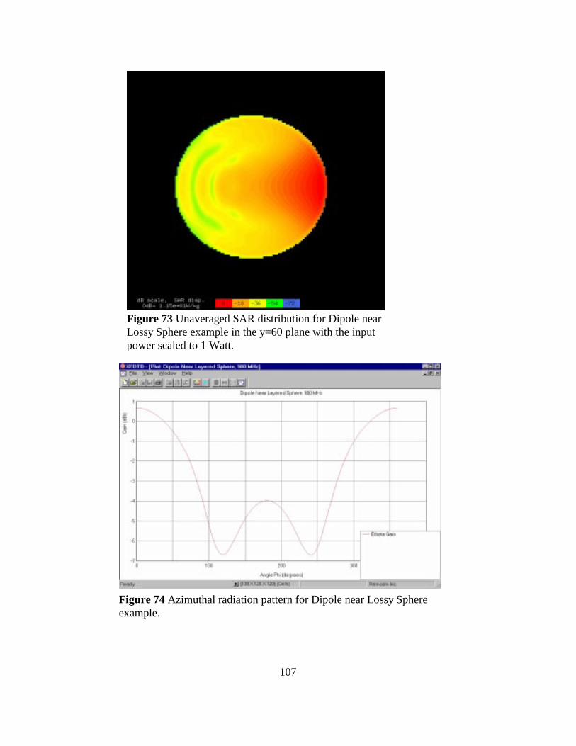
107

Figure 73 Unaveraged SAR distribution for Dipole nearLossy Sphere example in the y=60 plane with the inputpower scaled to 1 Watt.

Figure 74 Azimuthal radiation pattern for Dipole near Lossy Sphereexample.

108

14-5 CDROM Example Files

There are four groups of files on the XFDTD5.0 CDROM which include example resultsfor viewing. The various examples are discussed briefly here. Refer to the actualexample files for the results.

14-5-1 Antenna Examples

Cellular Telephone Example

These files contain an example of a detailed cellular telephone handset. Thedimensions and internal distribution of the telephone are designed to be similar to anactual telephone, but the internal components are not functional. The telephone has ahelical antenna which is simulated in XFDTD with a subgrid. To view both thephone and the helix, choose the "All grids" option for viewing.

The phone is fed with a 1.9 GHz sine wave. Several time-domain near-zone electricfields and current densities can be viewed with the plotting tools. There are also twofield sequences for watching movies of the field propagation. The steady-state inputimpedance, input and radiated power, efficiency and S parameters can be seenby selecting "Steady-State Data" from the Results menu.

Antenna patterns in any plane can be computed by selecting the Compute Far-Zonefrom the Results menu. Enter the desired pattern, add it to the list, and then press OK. The pattern can be viewed with the plotting tool by choosing Plots vs Angle.

Simple Subgrid Example - Helix on a Box

These files demonstrate the use of a subgrid by showing a simple PEC box in the maingrid and a helical antenna in the subgrid. Two cases are computed: a steady-statecalculation with a sine wave input, and a transient calculation with a broad-bandgaussian pulse input.

The steady-state example, helix.fdtd, displays field sequences in the main grid and inthe subgrid. The steady-state port information is available from theResults->Steady-State data menu. Antenna patterns in any plane may be computed byselecting Results->Compute Far-Zone Data. The antenna patterns may be view withthe plotting tools by selecting the plot versus angle option. Also available are thenear-zone field values at the feed versus time.

The broad-band example, helgaus.fdtd, also contains field sequences in both grids. The input impedance and S11 versus frequency may be plotted. Time domain data

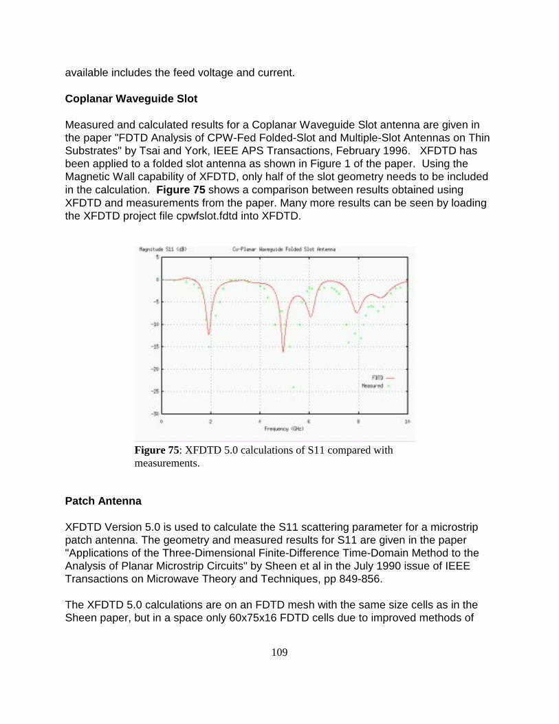
109

Figure 75: XFDTD 5.0 calculations of S11 compared withmeasurements.

available includes the feed voltage and current.

Coplanar Waveguide Slot

Measured and calculated results for a Coplanar Waveguide Slot antenna are given inthe paper "FDTD Analysis of CPW-Fed Folded-Slot and Multiple-Slot Antennas on ThinSubstrates" by Tsai and York, IEEE APS Transactions, February 1996. XFDTD hasbeen applied to a folded slot antenna as shown in Figure 1 of the paper. Using theMagnetic Wall capability of XFDTD, only half of the slot geometry needs to be includedin the calculation. Figure 75 shows a comparison between results obtained usingXFDTD and measurements from the paper. Many more results can be seen by loadingthe XFDTD project file cpwfslot.fdtd into XFDTD.

Patch Antenna

XFDTD Version 5.0 is used to calculate the S11 scattering parameter for a microstrippatch antenna. The geometry and measured results for S11 are given in the paper "Applications of the Three-Dimensional Finite-Difference Time-Domain Method to theAnalysis of Planar Microstrip Circuits" by Sheen et al in the July 1990 issue of IEEETransactions on Microwave Theory and Techniques, pp 849-856.

The XFDTD 5.0 calculations are on an FDTD mesh with the same size cells as in theSheen paper, but in a space only 60x75x16 FDTD cells due to improved methods of

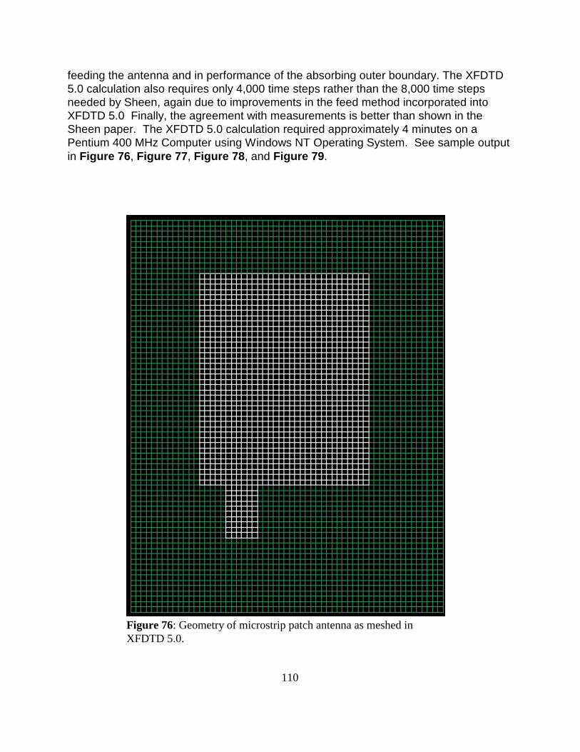
110

Figure 76: Geometry of microstrip patch antenna as meshed inXFDTD 5.0.

feeding the antenna and in performance of the absorbing outer boundary. The XFDTD5.0 calculation also requires only 4,000 time steps rather than the 8,000 time stepsneeded by Sheen, again due to improvements in the feed method incorporated intoXFDTD 5.0 Finally, the agreement with measurements is better than shown in theSheen paper. The XFDTD 5.0 calculation required approximately 4 minutes on aPentium 400 MHz Computer using Windows NT Operating System. See sample outputin Figure 76, Figure 77, Figure 78, and Figure 79.

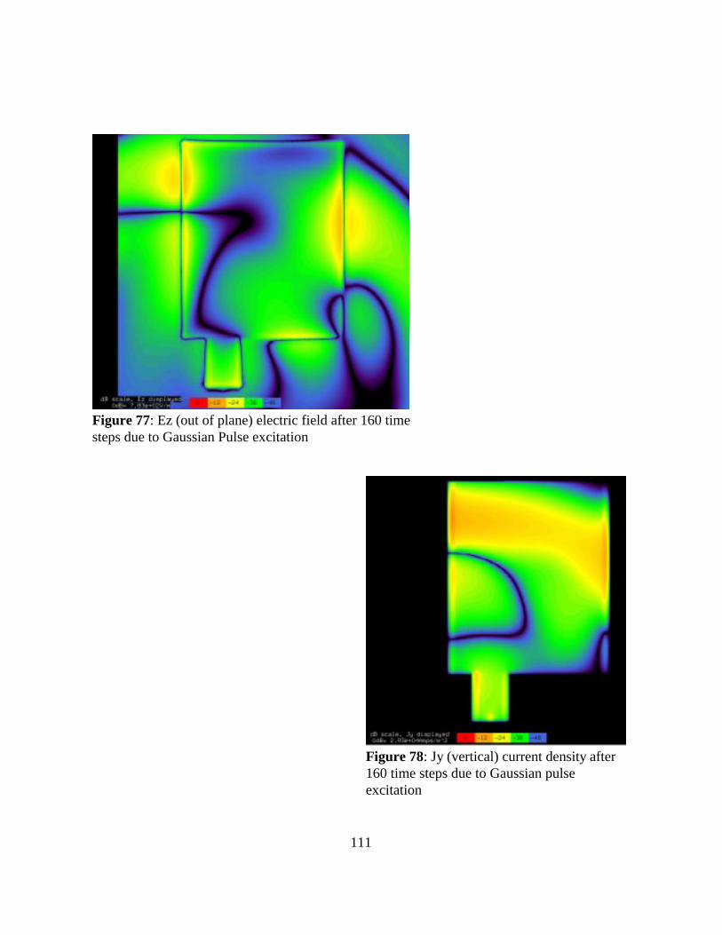
111

Figure 77: Ez (out of plane) electric field after 160 timesteps due to Gaussian Pulse excitation

Figure 78: Jy (vertical) current density after160 time steps due to Gaussian pulseexcitation

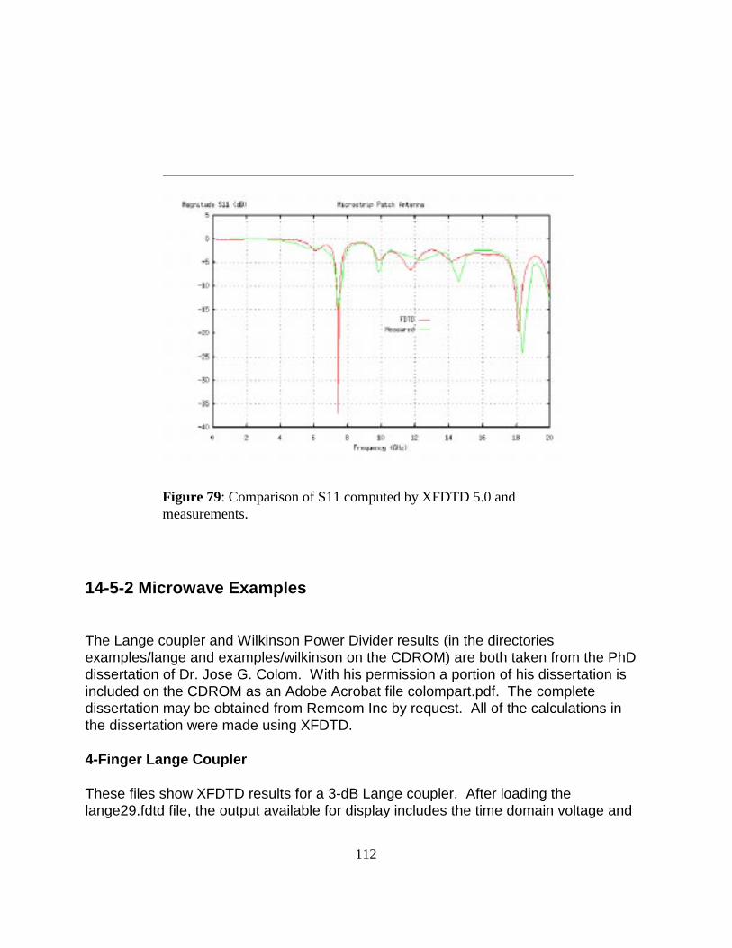
112

Figure 79: Comparison of S11 computed by XFDTD 5.0 andmeasurements.

14-5-2 Microwave Examples

The Lange coupler and Wilkinson Power Divider results (in the directoriesexamples/lange and examples/wilkinson on the CDROM) are both taken from the PhDdissertation of Dr. Jose G. Colom. With his permission a portion of his dissertation isincluded on the CDROM as an Adobe Acrobat file colompart.pdf. The completedissertation may be obtained from Remcom Inc by request. All of the calculations inthe dissertation were made using XFDTD.

4-Finger Lange Coupler

These files show XFDTD results for a 3-dB Lange coupler. After loading thelange29.fdtd file, the output available for display includes the time domain voltage and

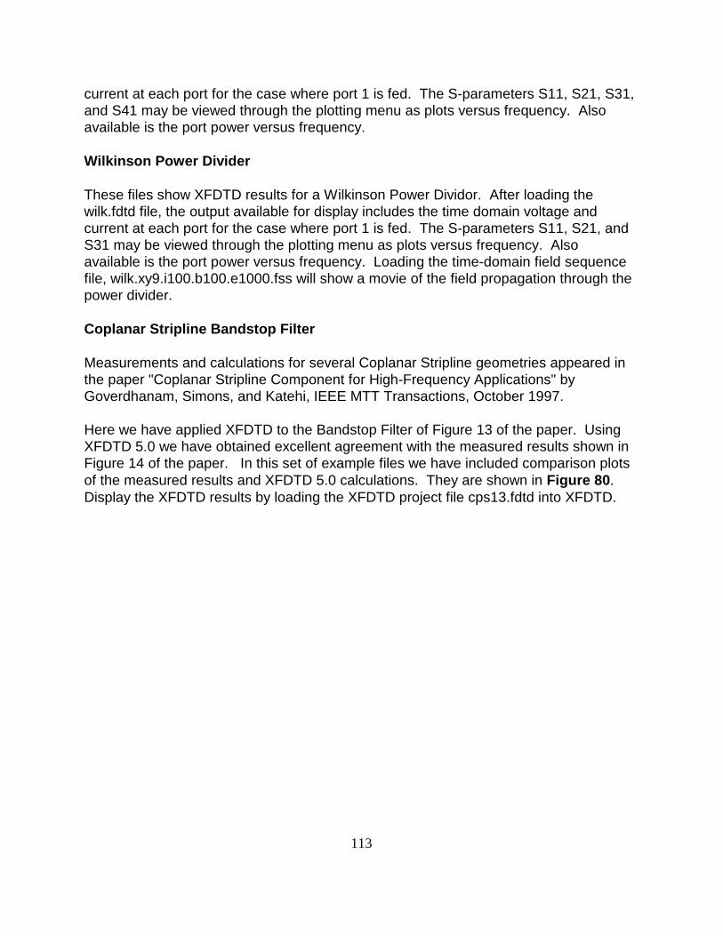
113

current at each port for the case where port 1 is fed. The S-parameters S11, S21, S31,and S41 may be viewed through the plotting menu as plots versus frequency. Alsoavailable is the port power versus frequency.

Wilkinson Power Divider

These files show XFDTD results for a Wilkinson Power Dividor. After loading thewilk.fdtd file, the output available for display includes the time domain voltage andcurrent at each port for the case where port 1 is fed. The S-parameters S11, S21, andS31 may be viewed through the plotting menu as plots versus frequency. Alsoavailable is the port power versus frequency. Loading the time-domain field sequencefile, wilk.xy9.i100.b100.e1000.fss will show a movie of the field propagation through thepower divider.

Coplanar Stripline Bandstop Filter

Measurements and calculations for several Coplanar Stripline geometries appeared inthe paper "Coplanar Stripline Component for High-Frequency Applications" byGoverdhanam, Simons, and Katehi, IEEE MTT Transactions, October 1997.

Here we have applied XFDTD to the Bandstop Filter of Figure 13 of the paper. UsingXFDTD 5.0 we have obtained excellent agreement with the measured results shown inFigure 14 of the paper. In this set of example files we have included comparison plotsof the measured results and XFDTD 5.0 calculations. They are shown in Figure 80. Display the XFDTD results by loading the XFDTD project file cps13.fdtd into XFDTD.

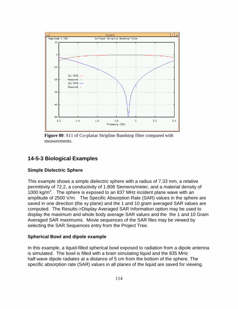
114

Figure 80: S11 of Co-planar Stripline Bandstop filter compared withmeasurements.

14-5-3 Biological Examples

Simple Dielectric Sphere

This example shows a simple dielectric sphere with a radius of 7.33 mm, a relativepermittivity of 72.2, a conductivity of 1.808 Siemens/meter, and a material density of1000 kg/m3. The sphere is exposed to an 837 MHz incident plane wave with anamplitude of 2500 V/m. The Specific Absorption Rate (SAR) values in the sphere aresaved in one direction (the xy plane) and the 1 and 10 gram averaged SAR values arecomputed. The Results->Display Averaged SAR Information option may be used todisplay the maximum and whole body average SAR values and the the 1 and 10 GramAveraged SAR maximums. Movie sequences of the SAR files may be viewed byselecting the SAR Sequences entry from the Project Tree.

Spherical Bowl and dipole example

In this example, a liquid-filled spherical bowl exposed to radiation from a dipole antennais simulated. The bowl is filled with a brain simulating liquid and the 835 MHzhalf-wave dipole radiates at a distance of 5 cm from the bottom of the sphere. Thespecific absorption rate (SAR) values in all planes of the liquid are saved for viewing.

115

Movies of the SAR through the liquid may be created. The SAR data is available foraveraging using the Results->Compute SAR statistics menu. The maximum,whole-body average and maximum 1 and 10 Gram averaged SAR values are available(after computing the SAR statistics) from the Results->Display SAR Information menu.Additionally, some data regarding the dipole is available including the steady-stateinput impedance, input power and efficiency, and the S11 values at the input frequency. Antenna patterns of the dipole/sphere geometry may be computed, if desired.

Comparisons of XFDTD impedance and SAR simulations of this geometry withexperimental data is available in the report "Measurements and FDTD Computations ofthe IEEE SCC 34 Spherical Bowl and Dipole Antenna" by Martin Siegbahn and ChristerTornevik of Ericsson Radio Systems. This report is included with the CDROM as anAdobe Acrobat file called ericsson.pdf

116

15 Trouble Shooting

The XFDTD programs have been extensively tested and should operate reliably on allsupported platforms. Should you encounter any difficulties you may contact Remcom,Inc by phone, fax or electronic mail.

REMCOM, Inc.Calder SquarePO Box 10023State College, PA 16805Phone: 814-353-2986Fax: 814-353-1420E-mail: [email protected]: http://www.remcom.com Before contacting us, however, please consider the following difficulties that may ariseand the suggested remedies.

15-1 Problems with XFDTD 5.0 on Windows

* Colors on screen are incorrect on Windows 98

There are some problems with Video acceleration for some cards with Windows 98. Todisable the acceleration, from the desktop click on Properties->Settings->Advanced->Performance and set Hardware Acceleration to “none”.

15-2 Problems with XFDTD 5.0 on Unix

* xfdtd50 and/or calcfdtd50 will not execute

Possibly the files are not set as executable. Use Unix chmod command.

* xfdtd50 gives a message about missing libraries (On Sun Solaris)

On some computers running the Sun Solaris operating system the path to the Motiflibraries must be in the LD_LIBRARY_PATH declaration.

117

For the C-Shell: edit the .cshrc file in your home directory, search for theLD_LIBRARY_PATH variable. Add /usr/dt/lib to this line.

EXAMPLE:setenv LD_LIBRARY_PATH $OPENWINHOME/lib:/usr/new/X11R5/lib:/usr/lib:/usr/dt/lib

For the K-Shell: edit the .profile file in your home directory, searchfor the LD_LIBRARY_PATH variable. Add the /usr/dt/lib to this line.

EXAMPLE:LD_LIBRARY_PATH=/usr/openwin/lib:/usr/ucblib:/usr/4lib:/usr/lib:/usr/dt/lib

* xfdtd50 and/or calcfdtd50 write license problem message to screen and stop

For Unix installation, check that license procedure was followed and thatxfdtd5.0.license and calcfdtd5.0.license files exist in /etc directory and contain only thelicense number supplied by Remcom, NOT your computer serial number. ContactRemcom, Inc for correct license number if necessary. This applies only to the Remcomsupplied licensing. If a special licensing situation, such as FlexLM is being used, thismessage does not apply.

* XFDTD colors appear strange or some materials are not visible in the mesh

Other Unix applications may be using colors that are needed by XFDTD. Close allother applications running on the computer platform and start XFDTD again. After youstart XFDTD look at the window from which you gave the "xfdtd50" command. If thereis a Unix warning that not all colors could be allocated, then you still have anapplication running that is using some of the colors required by XFDTD.

* difficulty reading files with XFDTD

Unix allows a limited number of files in the same directory. Try to separate files fromdifferent XFDTD calculations into different directories.

* Can’t read files into XFDTD after Upgrade to Newer Version

XFDTD should be fully backward compatible. This means files created by olderversions of XFDTD should be functional with XFDTD 5.0. Files created by XFDTD 5.0

118

can not be read in older versions of XFDTD (2 - 4) since the formats are different. It isrecommended that when you receive your new version of XFDTD that you remove allthe XFDTD executable files from the previous version from your computer.

119

16 The Human Head and Shoulders FDTD Mesh

You may have received one of our FDTD meshes of a male human head andshoulders. This was created using digitized data in the form of transverse colorimages. The data is from the Visible Human Project sponsored by the National Libraryof Medicine (NLM) and is available via the Internet at no cost. For information browse

http://www.nlm.nih.gov/research/visible/visible_human.html

The male data set consists of MRI, CT and anatomical images. Axial MRI images ofthe head and neck and longitudinal sections of the rest of the body are available at 4mm intervals. The MRI images have 256 pixel by 256 pixel resolution. Each pixel has12 bits of gray tone resolution. The CT data consists of axial CT scans of the entirebody taken at 1 mm intervals at a resolution of 512 pixels by 512 pixels where eachpixel is made up of 12 bits of gray tone. The axial anatomical images are 2048 pixelsby 1216 pixels where each pixel is defined by 24 bits of color, about 7.5 megabytes. The anatomical cross sections are also at 1 mm intervals and coincide with the CT axialimages. There are 1871 cross sections for each mode, CT and anatomy. Thecomplete male data set is 15 gigabytes in size. Our mesh of the human head andshoulders used the axial anatomical images since these had the finest resolution.

16-1 The 3mm Head and Shoulders Mesh

The choice of the problem space dimensions came from consideration of the computerresources that would be required to make the calculation. An FDTD mesh of twomillion cells will require about 96 MBytes of RAM. A cell size of 3 mm was chosen forthe original mesh since it will allow the head and shoulders region, including a 20 cellborder, to be modeled in a space of 153 x 118 x 120 or 2,166,480 cells.

Creating the XFDTD .id file from the axial anatomical images

Each of the axial anatomical images contains .33 mm x .33 mm pixels. We sampleeach image every 9 x 9 pixels such that we represent an area 3 mm x 3 mm with onepixel or 24-bit value. We convert this 24-bit data value to a corresponding set ofconstitutive parameters by assigning tissues to five different tissue types. Each ofthese is also assigned a material type number in XFDTD. In addition we add a groupfor skin. It was not possible to separate skin from the other tissues from the files, so aone-to-two cell layer of skin was added manually.

This grouping or conversion process was done by inspection. Each 24-bit value thatcorresponds to an FDTD cell was originally examined with the help of [19,20] andproperly placed into one of the above six groups.

120

Dr. Michael Smith and Mr. Chris Collins of The Milton S. Hershey Medical Center,Hershey, Pa, reviewed the original FDTD mesh developed by Remcom, Inc., andrevised it. These revisions included improved fidelity, additional shoulder region, andremoval of small regions of blood which do not correspond to a living human, butpooled after the death of the human subject. Information about their research effortscan be obtained by browsing

http://nmr.hmc.psu.edu

The six groups of tissue types in the original mesh and their XFDTD material numbersare:

XFDTD #2 cartilageXFDTD #4 muscle XFDTD #7 eyeXFDTD #9 brainXFDTD #12 dry skinXFDTD #14 skull bone

These correspond roughly to the tissue groups of the entire body mesh, except that theentire body mesh: 1) has lung tissue and internal organs which are absent from thehead/shoulders mesh; 2) combines cartilage with fat and bone; and 3) includes blood.

For each tissue group we have found reasonable approximations to the material densityin kg/m3. In particular, the values given by Camelia Gabriel, Ph.D., and Sami Gabriel,M. Sc., Physics Department, Kings College London, London WC2R2LS, UK foraverage brain (1030), average skull (1850), and average muscle (1040) are used. Their values of conductivity in S/m and relative permittivity are also recommended forthe head/shoulders. The electrical constitutive parameters change with frequency, andcan be obtained from the www site:

http://www.brooks.af.mil/AL/OE/OER/Title/Title.html

which is supported by

Armstrong Laboratory (AFMC)Occupational and Environmental Health DirectorateRadiofrequency Radiation Division2503 D DriveBrooks AFBTX 78235-5102

Approximate values for different frequencies as given by Camelia Gabriel, Ph.D., and

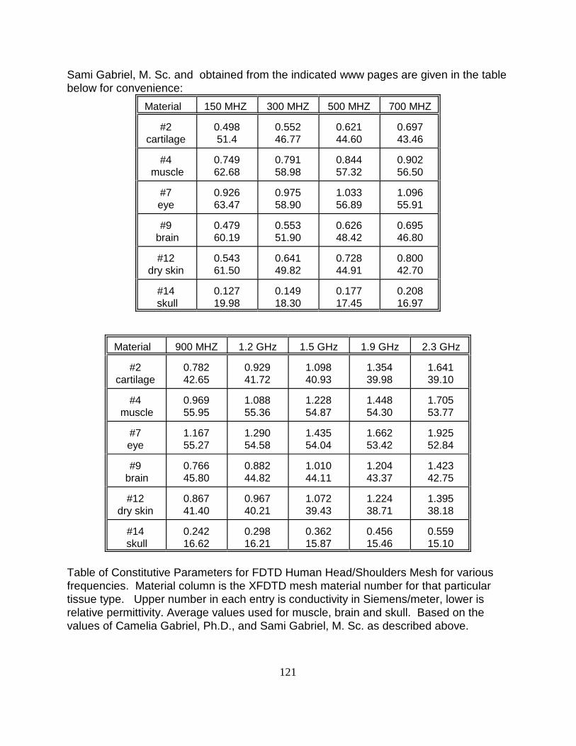
121

Sami Gabriel, M. Sc. and obtained from the indicated www pages are given in the tablebelow for convenience:

Material 150 MHZ 300 MHZ 500 MHZ 700 MHZ

#2cartilage

0.49851.4

0.55246.77

0.62144.60

0.69743.46

#4 muscle

0.74962.68

0.79158.98

0.84457.32

0.90256.50

#7eye

0.92663.47

0.97558.90

1.03356.89

1.09655.91

#9 brain

0.47960.19

0.55351.90

0.62648.42

0.69546.80

#12dry skin

0.54361.50

0.64149.82

0.72844.91

0.80042.70

#14 skull

0.12719.98

0.14918.30

0.17717.45

0.20816.97

Material 900 MHZ 1.2 GHz 1.5 GHz 1.9 GHz 2.3 GHz

#2cartilage

0.78242.65

0.92941.72

1.09840.93

1.35439.98

1.64139.10

#4 muscle

0.96955.95

1.08855.36

1.22854.87

1.44854.30

1.70553.77

#7eye

1.16755.27

1.29054.58

1.43554.04

1.66253.42

1.92552.84

#9 brain

0.76645.80

0.88244.82

1.01044.11

1.20443.37

1.42342.75

#12dry skin

0.86741.40

0.96740.21

1.07239.43

1.22438.71

1.39538.18

#14 skull

0.24216.62

0.29816.21

0.36215.87

0.45615.46

0.55915.10

Table of Constitutive Parameters for FDTD Human Head/Shoulders Mesh for variousfrequencies. Material column is the XFDTD mesh material number for that particulartissue type. Upper number in each entry is conductivity in Siemens/meter, lower isrelative permittivity. Average values used for muscle, brain and skull. Based on thevalues of Camelia Gabriel, Ph.D., and Sami Gabriel, M. Sc. as described above.

122

16-2 The Remcom High-Fidelity Head and Shoulders Mesh

The Remcom High-Fidelity Head and Shoulders mesh is based on the same data asused in the 3mm mesh, but it uses 2x2x2.5 mm cells and has dimensions 309x177x161for 8,805,573 cells. It contains 17 materials which are assigned as follows:

XFDTD #2 SkinXFDTD #3 TendonXFDTD #4 Fat/Yellow MarrowXFDTD #5 Cortical BoneXFDTD #6 Cancellous BoneXFDTD #7 BloodXFDTD #8 MuscleXFDTD #9 Grey Matter XFDTD #10 White MatterXFDTD #11 Cerebro-spinal fluid XFDTD #12 Sclera/CorneaXFDTD #13 Vitreous HumorXFDTD #15 NerveXFDTD #16 CartilageXFDTD #17 Tongue/ThyroidXFDTD #19 CerebellumXFDTD #20 Esophagus

Measured values for the tissue parameters for a broad frequency range from 1 MHz to20 Ghz are included with the mesh data. The tissue parameters may be adjustedautomatically for a specific frequency by using the Edit->Adjust Tissue MaterialParameters menu. The correct values from the table of measured data will be selectedand entered into the appropriate mesh variables. The mesh must be saved afteradjusting the parameters for the new values to be used in the XFDTD calculation butthe parameters can be adjusted as many times as required.

123

17 The Human Body FDTD Mesh

You may have received one of our FDTD meshes of a male human body. They werecreated using digitized data in the form of transverse color images. The data is fromthe Visible Human Project sponsored by the National Library of Medicine (NLM) and isavailable via the Internet at no cost. The male data set consists of MRI, CT andanatomical images. Axial MRI images of the head and neck and longitudinal sectionsof the rest of the body are available at 4 mm intervals. The MRI images have 256 pixelby 256 pixel resolution. Each pixel has 12 bits of gray tone resolution. The CT dataconsists of axial CT scans of the entire body taken at 1 mm intervals at a resolution of512 pixels by 512 pixels where each pixel is made up of 12 bits of gray tone. The axialanatomical images are 2048 pixels by 1216 pixels where each pixel is defined by 24bits of color, about 7.5 megabytes. The anatomical cross sections are also at 1 mmintervals and coincide with the CT axial images. There are 1871 cross sections foreach mode, CT and anatomy. The complete male data set is 15 gigabytes in size. Ourmesh of the human body required the axial anatomical images since these had thefinest resolution of the entire body.

17-1 The Original 5mm Body Mesh

The choice of the problem space dimensions came from consideration of the computerresources that would be required to make the calculation. An FDTD mesh of six millioncells will require about 180 MBytes of RAM and about 6 hours of run time on a fastwork station. A cell size of 5 mm was chosen since it will allow the entire human bodyincluding a 20 cell border to be modeled in a space of 157x102x396 or 6,341,544 cells.

Creating the XFDTD .id file from the axial anatomical images

Each of the axial anatomical images contains .33 mm x .33 mm pixels. We sampleeach image every 15 x 15 pixels such that we represent an area 5 mm x 5 mm with onepixel or 24-bit value. We convert this 24-bit data value to a corresponding set ofconstitutive parameters by assigning tissues to six different tissue types. Each of theseis also assigned a material type number in XFDTD. The six groups of tissue types andtheir XFDTD material numbers are

group 1 XFDTD #14 fat, bone, cartilagegroup 2 XFDTD #4 intestine, liver, kidney, muscle, spleen, pancreas, skingroup 3 XFDTD #9 nerve, braingroup 4 XFDTD #7 eyegroup 5 XFDTD #15 bloodgroup 6 XFDTD #13 lung

This grouping or conversion process was done by inspection. Each 24-bit value that

124

corresponds to an FDTD cell must be examined with the help of [19,20] and properlyplaced into one of the above six groups.

For each tissue group we have found reasonable approximations to the material densityin kg/m**3, conductivity (sig) in S/m and relative permittivity. The electrical constitutiveparameters change with frequency, and values for 5 different frequencies are given inthe table:

Constitutive Parameters for FDTD Human Body Mesh

tissue type density 150 MHZ 300 MHZ 500 MHZ 700 and 915 MHZ kg/m3 sig, eps sig, eps sig, eps sig, eps

fat, bone 1130 .07, 6.7 .09, 8.3 .07, 5.1 .07, 5.1cartilage

intestine, 1020 .88, 69 .92 ,57 .85, 56 1.0, 52.6liver,kidney,muscle,spleen,pancreas,skin

nerve, brain 1050 .57, 72 .61, 55 .7, 46 .75, 44 eye 1000 1.9,84 1.7,74 1.9,70 1.9, 70 blood 1000 1.12, 70 1.19, 74 1.09, 63 1.18, 62

lung 330 .28, 22 .22, 12 .24, 12 .24, 12

sig=conductivity in Siemens/m eps=relative permittivity

17-2 The Remcom High-Fidelity Body Mesh

The Remcom High-Fidelity Body mesh is based on the same data as used in theoriginal mesh. It uses 5x5x5 mm cells and has dimensions 136x87x397 for 4,697304cells. The High-Fidelity mesh is much more detailed than the original mesh and itcontains 23 materials which are assigned as follows:

125

XFDTD #2 SkinXFDTD #3 Tendon, pancreas, prostate, aorta, liver, otherXFDTD #4 Fat/Yellow MarrowXFDTD #5 Cortical BoneXFDTD #6 Cancellous BoneXFDTD #7 BloodXFDTD #8 Muscle, heart, spleen, colon, tongueXFDTD #9 Grey Matter, cerebellumXFDTD #10 White MatterXFDTD #11 Cerebro-spinal fluid XFDTD #12 Sclera/CorneaXFDTD #13 Vitreous HumorXFDTD #14 BladderXFDTD #15 NerveXFDTD #16 CartilageXFDTD #18 Gall Bladder bileXFDTD #19 ThyroidXFDTD #20 Stomach, EsophagusXFDTD #21 LungXFDTD #22 KidneyXFDTD #24 TestesXFDTD #25 LensXFDTD #27 Small intestine

Measured values for the tissue parameters for a broad frequency range are includedwith the mesh data. The tissue parameters may be adjusted automatically for a specificfrequency by using the Edit->Adjust Tissue Material Parameters menu. The correctvalues from the table of measured data will be selected and entered into theappropriate mesh variables. The mesh must be saved after adjusting the parametersfor the new values to be used in the XFDTD calculation but the parameters can beadjusted as many times as required.

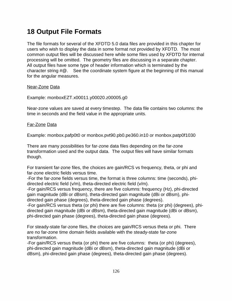
126

18 Output File Formats

The file formats for several of the XFDTD 5.0 data files are provided in this chapter forusers who wish to display the data in some format not provided by XFDTD. The mostcommon output files will be discussed here while some files used by XFDTD for internalprocessing will be omitted. The geometry files are discussing in a separate chapter.All output files have some type of header information which is terminated by thecharacter string #@. See the coordinate system figure at the beginning of this manualfor the angular measures.

Near-Zone Data

Example: monboxEZT.x00011.y00020.z00005.g0

Near-zone values are saved at every timestep. The data file contains two columns: thetime in seconds and the field value in the appropriate units.

Far-Zone Data

Example: monbox.pafp0t0 or monbox.pvt90.pb0.pe360.in10 or monbox.patp0f1030

There are many possibilities for far-zone data files depending on the far-zonetransformation used and the output data. The output files will have similar formatsthough.

For transient far-zone files, the choices are gain/RCS vs frequency, theta, or phi andfar-zone electric fields versus time. -For the far-zone fields versus time, the format is three columns: time (seconds), phi-directed electric field (v/m), theta-directed electric field (v/m). -For gain/RCS versus frequency, there are five columns: frequency (Hz), phi-directedgain magnitude (dBi or dBsm), theta-directed gain magnitude (dBi or dBsm), phi-directed gain phase (degrees), theta-directed gain phase (degrees).-For gain/RCS versus theta (or phi) there are five columns: theta (or phi) (degrees), phi-directed gain magnitude (dBi or dBsm), theta-directed gain magnitude (dBi or dBsm),phi-directed gain phase (degrees), theta-directed gain phase (degrees).

For steady-state far-zone files, the choices are gain/RCS versus theta or phi. Thereare no far-zone time domain fields available with the steady-state far-zonetransformation.-For gain/RCS versus theta (or phi) there are five columns: theta (or phi) (degrees),phi-directed gain magnitude (dBi or dBsm), theta-directed gain magnitude (dBi ordBsm), phi-directed gain phase (degrees), theta-directed gain phase (degrees).

127

S-parameter Data

Example: monbox.s11 or monbox.ss.s11

For transient S-parameter calculations, the file has five columns: frequency (Hz), thereal part, the imaginary part, the magnitude (dB), and the phase (degrees).

For steady-state S-parameters, there is only a single line of data in the same format asabove.

Transient Field Data

Example: monbox.xz12.t200.fld

These are the field snapshot which show the electric and magnetic fields or currentdensity in a plane at various moments in time. The file has a header which containsfive lines. Below is an example with the definitions of each item.

t - means the file contains total field data. This is always the case.80 1200 3 18 0 - timestep number, maximum timestep number, slice direction (1=xy,2=yz, 3=xz), the slice number (which is always one less than what is shown in XFDTD),and the grid number (0=main grid, 1=subgrid 1, etc)67 37 91 - the dimensions of the space in cells3.216099e+00 - the timestep in picoseconds1.670000e-03 1.670000e-03 1.670000e-03 - the spatial increments of the geometry

Following this header, there are 9 floating point numbers for every cell in the spacestarting in the lowest corner and working up to the highest. So, if this is the xz plane,the first point will be for x=1, z=1. The loop will be as follows:

from z=1 to maximum z From x=1 to maximum x Write -> Ex, Ey, Ez, Hx, Hy, Hz, Jx, Jy, JzIn the xy plane it will be:

from y=1 to maximum y From x=1 to maximum x Write -> Ex, Ey, Ez, Hx, Hy, Hz, Jx, Jy, JzIn the yz plane it will be:

from z=1 to maximum z From y=1 to maximum y Write -> Ex, Ey, Ez, Hx, Hy, Hz, Jx, Jy, Jz

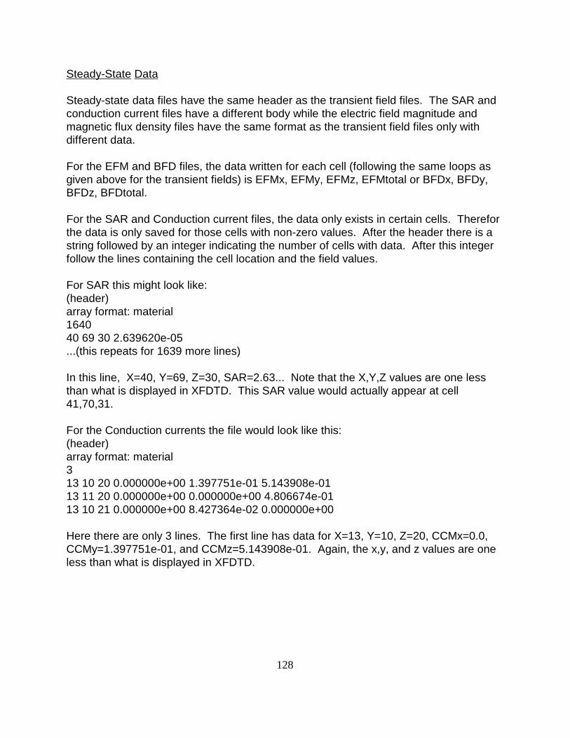
128

Steady-State Data

Steady-state data files have the same header as the transient field files. The SAR andconduction current files have a different body while the electric field magnitude andmagnetic flux density files have the same format as the transient field files only withdifferent data.

For the EFM and BFD files, the data written for each cell (following the same loops asgiven above for the transient fields) is EFMx, EFMy, EFMz, EFMtotal or BFDx, BFDy,BFDz, BFDtotal.

For the SAR and Conduction current files, the data only exists in certain cells. Thereforthe data is only saved for those cells with non-zero values. After the header there is astring followed by an integer indicating the number of cells with data. After this integerfollow the lines containing the cell location and the field values.

For SAR this might look like:(header)array format: material164040 69 30 2.639620e-05 ...(this repeats for 1639 more lines)

In this line, X=40, Y=69, Z=30, SAR=2.63... Note that the X,Y,Z values are one lessthan what is displayed in XFDTD. This SAR value would actually appear at cell41,70,31.

For the Conduction currents the file would look like this:(header)array format: material313 10 20 0.000000e+00 1.397751e-01 5.143908e-0113 11 20 0.000000e+00 0.000000e+00 4.806674e-01 13 10 21 0.000000e+00 8.427364e-02 0.000000e+00

Here there are only 3 lines. The first line has data for X=13, Y=10, Z=20, CCMx=0.0,CCMy=1.397751e-01, and CCMz=5.143908e-01. Again, the x,y, and z values are oneless than what is displayed in XFDTD.

129

19 References

7 K. Kunz and R. Luebbers, The Finite Difference Time Domain Method forElectromagnetics, 1993, CRC Press Catalog Number 8657, 496 pages.

8 T. Iwasaki, A. P. Freundorfer, K. Iizuka, "A unidirectional semi-circular spiralantenna for subsurface radars," IEEE Trans. Electromagn. Compat., vol. 36, pp1-6, Feb. 1994

9 J. D. Dyson, "The equiangular spiral antenna," IRE Trans. Antenna Propagat.,vol 7, pp 181-187, April 1959.

10 H. Nakano, K. Nogami, S. Arai, H. Mimaki, and J. Yamauchi, "A spiral antennabacked by a conducting plane reflector," IEEE Trans. Antennas Propagat., vol.34, pp 791-796, June 1986.

11 K. Chamberlin and L. Gordon, “Modeling Good Conductors Using the FiniteDifference Time Domain Technique,” IEEE Trans. EMC, vol 37, no. 2, pp210-216, 1995.

12 C. A. Balanis, Advanced Engineering Electromagnetics, Section 2.8.3

13 Ramo, Whinnery and Van Duzer, Fields and Waves in CommunicationElectronics, Section 13.12

14 R. E Collin, Foundations for Microwave Engineering, Section 6.7

15 B. Lax and K. J. Button, Microwave Ferrites and Ferrimagnetics, Sections 4.1 -4.2

16 Z. P. Liao, H. L. Wong, G. P. Yang, and Y. F. Yuan, "A transmitting boundary fortransient wave analysis," Scientia Sinica, vol. 28, no. 10, pp 1063-1076, Oct.1984.

17 J.P. Berenger, "A perfectly matched layer for the absorption of electromagneticwaves," J. Computat. Phys., Oct. 1994

18 J. Basterrechea and M. F. Cátedra, “Computation of Microstrip S-parametersusing a CG-FFT Scheme,” IEEE Transactions on Microwave Theory andTechniques, vol. 42, no. 2, pp 234-240, February 1994.

19 Robert S. Ledlet, H. K. Huang, and John C. Mazziotta, "Cross-Section Anatomy -An Atlas for Computerized Tomography," The Williams and Wilkins Co., 1977

130

20 Richard A. Boolootian, "Elements of Human Anatomy and Physiology," WestPublishing Co., 1976

20 Bibliography

K. Kunz, R. Luebbers, The Finite Difference Time Domain Method for Electromagnetics,CRC Press, 496 pp, 1993.

R. Luebbers, K. S. Kunz, K. A. Chamberlin, "An Interactive Demonstration ofElectromagnetic Wave Propagation Using Time-Domain Finite Differences", IEEETransactions on Education, vol 33, no 1, pp 60-68, February 1990.

R. Luebbers, F. Hunsberger, K. Kunz, R. Standler, "A Frequency-Dependent FiniteDifference Time Domain Formulation for Dispersive Materials", IEEE Transactions onElectromagnetic Compatibility, vol 32, no 3, pp 222-227, August 1990.

K. Kunz, R. Luebbers, F. Hunsberger, "A Thin Dipole Antenna Demonstration of theAntenna Modeling Capabilities of the Finite Difference Time Domain Technique",Applied Computational Electromagnetics Society Journal, vol 5, no 1, pp 2-18, Summer1990.

R. Luebbers, F. Hunsberger, K. Kunz, "A Frequency-Dependent Time DomainFormulation for Transient Propagation in Plasma", IEEE Transactions on Antennas andPropagation, vol 39, no 1, pp 29-34, January 1991.

R. Luebbers, K. Kunz, M. Schneider, F. Hunsberger, "A Finite Difference Time DomainNear-Zone to Far-Zone Transformation", IEEE Transactions on Antennas andPropagation, vol 39, no 4, pp 429-433, April 1991.

J. Beggs, R. Luebbers, K. S. Yee, K. Kunz, "Finite Difference Time DomainImplementation of Surface Impedance Boundary Conditions", IEEE Transactions onAntennas and Propagation, vol 40, no 1, pp 49-56, January 1992.

R. Luebbers, K. Kunz, "FDTD Modeling of Thin Impedance Sheets", IEEE Transactionson Antennas and Propagation, vol 40, no 3, pp 349-351, March 1992.

R. Luebbers, K. Kunz, "Finite Difference Time Domain Calculations of Antenna MutualCoupling", IEEE Transactions on Electromagnetic Compatibility, vol 34, no 3, pp357-360, August 1992.

131

R. Luebbers, F. Hunsberger, "FDTD for Nth Order Dispersive Media," IEEETransactions on Antennas and Propagation, vol 40, no 11, pp 1297-1301, November1992.

R. Luebbers, J. Beggs, "FDTD Calculation of Wide-Band Antenna Gain and Efficiency,"IEEE Transactions on Antennas and Propagation, vol 40, no 11, pp 1404-1407,November 1992.

F. Hunsberger, R. Luebbers and K. Kunz, "Finite-Difference Time-Domain Analysis ofGyrotropic Media I: Magnetized Plasma," IEEE Transactions on Antennas andPropagation, vol 40, no 12, pp 1489-1495, December 1992.

R. Luebbers, L. Chen, T. Uno, and S. Adachi, "FDTD Calculation of Radiation Patterns,Impedance and Gain for a Monopole Antenna on a Conducting Box," IEEETransactions on Antennas and Propagation, vol 40, no 12, pp 1577-1583, December1992.

R. Luebbers, T. Uno, K. Kumagai, "Pulse Propagation in a Linear, Causally DispersiveMedium," Proceedings of the IEEE, vol. 81, no 4, pp 631-636, April 1993.

R. Luebbers, J. Beggs, K. Chamberlin, "Finite Difference Time Domain Calculation ofTransients in Antennas with Nonlinear Loads", IEEE Transactions on Antennas andPropagation, vol 41, no 5, pp 566-573, May 1993.

R. Luebbers, D. Steich, and K. Kunz, "FDTD Calculation of Scattering from Frequency-Dependent Materials," IEEE Transactions on Antennas and Propagation, vol 41, no 9,pp 1249- 1257, September 1993.

J. Beggs, R. Luebbers, and B. Ruth, "Analysis of Electromagnetic Radiation fromShaped-End Radiators using the Finite Difference Time Domain Method," IEEETransactions on Antennas and Propagation, vol 41, no 9, pp 1324-1327, September1993.

R. Luebbers, "Lossy Dielectrics in FDTD," IEEE Transactions on Antennas andPropagation, vol 41, no 11, pp 1586-1588, November 1993.

C. Penney and R. Luebbers, "Radiation and Scattering of a Square Archimedean SpiralAntenna using FDTD," Electromagnetics, vol 14, no 1, pp 87-98, January-March 1994.

R. Luebbers and C. Penney, "Scattering from Apertures in Infinite Ground Planes usingFDTD," IEEE Transactions on Antennas and Propagation, vol 42, no 5, pp 731-737,May 1994.

132

C. Penney and R. Luebbers, "Input Impedance, Radiation Pattern, and Radar CrossSection of Spiral Antennas using FDTD," IEEE Transactions on Antennas andPropagation, vol 42, no 9, pp 1328-1333, September 1994.

R. Luebbers, "Three-Dimensional Cartesian-Mesh Finite-Difference Time-DomainCodes," IEEE Antennas and Propagation Magazine, vol 36, no 6, pp 66-71, December1994.

D. Steich, R. Luebbers, K. Kunz, "Absorbing Boundary Condition ConvergenceComparisons," IEEE Antennas and Propagation Society International Symposium, AnnArbor, MI, June 28-July 2, 1993.

D. F. Kelley, R. Luebbers, "Comparison of Dispersive Media Modeling Techniques inthe Finite Difference Time Domain Method," IEEE Antennas and Propagation SocietyInternational Symposium, Seattle, WA, June 19-24, 1994.

J. Schuster, R. Luebbers, "Application of FDTD to Anisotropic Materials," IEEEAntennas and Propagation Society International Symposium, Seattle, WA, June 19-24,1994.

R. Luebbers and H. S. Langdon, "Reducing the Number of Time Steps Needed forFDTD Antenna and Microstrip Calculations," 11th Annual Review of Progress inApplied Computational Electromagnetics, Naval Postgraduate School, Monterey, CA,March 20-25, 1995.

D. F. Kelley and R. Luebbers, "The Piecewise Linear Recursive Convolution Method forIncorporating Dispersive Media into FDTD," 11th Annual Review of Progress in AppliedComputational Electromagnetics, Naval Postgraduate School, Monterey, CA, March20-25, 1995.

J. Schuster and R. Luebbers, "Application of the FDTD Method to Three-DimensionalPropagation in a Magnetized Ferrite, 12th Annual Review of Progress in AppliedComputational Electromagnetics, Naval Postgraduate School, Monterey, CA, March18-22, 1996.

C. Penney, R. Luebbers, and J. Schuster. "Scattering from Coated Targets Using aFrequency-Dependent, Surface Impedance Boundary Condition," IEEE Transactions onAntennas and Propagation, vol 44, no 4, pp 434-443, April 1996.

D. Kelley, R. Luebbers, "Piecewise Linear Recursive Convolution for Dispersive Mediausing FDTD," IEEE Transactions on Antennas and Propagation, vol 44, no 6, pp 792-798, June 1996.

133

M. Chevalier and R. Luebbers, "FDTD Subgrid with Material Traverse," IEEE AP-SInternational Symposium and URSI Radio Science Meeting, Baltimore, MD, July 21-26,1996.

J. Schuster, R. Luebbers and H. Riazi, "FDTD Predictions and Measurements of CarEffects on Portable Telephone Received Signal Levels," IEEE AP-S InternationalSymposium and URSI Radio Science Meeting, Baltimore, MD, July 21-26, 1996.

R. Luebbers, "Thirty Years After: Kane Yee and FDTD," IEEE AP-S InternationalSymposium and URSI Radio Science Meeting, Baltimore, MD, July 21-26, 1996.

J. Schuster, R. Luebbers, "Comparison of Site-Specific Radio Propagation Path LossPredictions to Measurements in an Urban Area," IEEE AP-S International Symposiumand URSI Radio Science Meeting, Baltimore, MD, July 21-26, 1996.

J. Schuster, R. Luebbers, "FDTD for Three-Dimensional Propagation in a MagnetizedFerrite," IEEE AP-S International Symposium and URSI Radio Science Meeting,Baltimore, MD, July 21-26, 1996.

D. Kelley, R. Luebbers, "Calculation of Dispersion Errors for the Piecewise-LinearRecursive Convolution Method," IEEE AP-S International Symposium and URSI RadioScience Meeting, Baltimore, MD, July 21-26, 1996.

R. Luebbers, R. Baurle, "FDTD Predictions of Electromagnetic Field in and near HumanBodies using Visible Human Project Anatomical Scans," IEEE AP-S InternationalSymposium and URSI Radio Science Meeting, Baltimore, MD, July 21-26, 1996.

R. Luebbers and H. S. Langdon, "A Simple Feed Model that Reduces Time StepsNeeded for FDTD Antenna and Microstrip Calculations," IEEE Transactions onAntennas and Propagation, vol 44, no 7, pp 1000-1005, July 1996.

J. W. Schuster and R. Luebbers, "Finite difference time domain analysis of arbitrarilybiased magnetized ferrites," Radio Science, vol 34, no. 4, pp 923-930, July-August1996.

M. Chevalier, R. Luebbers, and V. Cable, “FDTD Local grid with Material Traverse,”IEEE Transactions on Antennas and Propagation, vol 45, no 3, pp 411-421, March1997.

Documents

XFDTDcfurse/Tutorials/XFDTD/man50492.pdf7 1-2-2 Define Project Parameters Once the geometry is defined, the FDTD calculation parameters for the specific project are chosen. These parameters