Embed Size (px)
Citation preview
Atmos. Chem. Phys., 12, 2313–2343, 2012www.atmos-chem-phys.net/12/2313/2012/doi:10.5194/acp-12-2313-2012© Author(s) 2012. CC Attribution 3.0 License.
AtmosphericChemistry
and Physics
Xenon-133 and caesium-137 releases into the atmosphere from theFukushima Dai-ichi nuclear power plant: determination of thesource term, atmospheric dispersion, and deposition
A. Stohl1, P. Seibert2, G. Wotawa3, D. Arnold2,4, J. F. Burkhart 1, S. Eckhardt1, C. Tapia5, A. Vargas4, andT. J. Yasunari6
1NILU – Norwegian Institute for Air Research, Kjeller, Norway2Institute of Meteorology, University of Natural Resources and Life Sciences, Vienna, Austria3Central Institute for Meteorology and Geodynamics, Vienna, Austria4Institute of Energy Technologies (INTE), Technical University of Catalonia (UPC), Barcelona, Spain5Department of Physics and Nucelar Engineering (FEN),Technical University of Catalonia (UPC), Barcelona, Spain6Universities Space Research Association, Goddard Earth Sciences and Technology and Research, Columbia,MD 21044, USA
Correspondence to:A. Stohl ([email protected])
Received: 8 October 2011 – Published in Atmos. Chem. Phys. Discuss.: 20 October 2011Revised: 1 February 2012 – Accepted: 23 February 2012 – Published: 1 March 2012
Abstract. On 11 March 2011, an earthquake occurred about130 km off the Pacific coast of Japan’s main island Honshu,followed by a large tsunami. The resulting loss of electricpower at the Fukushima Dai-ichi nuclear power plant de-veloped into a disaster causing massive release of radioac-tivity into the atmosphere. In this study, we determine theemissions into the atmosphere of two isotopes, the noblegas xenon-133 (133Xe) and the aerosol-bound caesium-137(137Cs), which have very different release characteristics aswell as behavior in the atmosphere. To determine radionu-clide emissions as a function of height and time until 20April, we made a first guess of release rates based on fuelinventories and documented accident events at the site. Thisfirst guess was subsequently improved by inverse modeling,which combined it with the results of an atmospheric trans-port model, FLEXPART, and measurement data from severaldozen stations in Japan, North America and other regions.We used both atmospheric activity concentration measure-ments as well as, for137Cs, measurements of bulk deposi-tion. Regarding133Xe, we find a total release of 15.3 (un-certainty range 12.2–18.3) EBq, which is more than twice ashigh as the total release from Chernobyl and likely the largestradioactive noble gas release in history. The entire noble gasinventory of reactor units 1–3 was set free into the atmo-sphere between 11 and 15 March 2011. In fact, our releaseestimate is higher than the entire estimated133Xe inventory
of the Fukushima Dai-ichi nuclear power plant, which weexplain with the decay of iodine-133 (half-life of 20.8 h) into133Xe. There is strong evidence that the133Xe release startedbefore the first active venting was made, possibly indicatingstructural damage to reactor components and/or leaks due tooverpressure which would have allowed early release of no-ble gases. For137Cs, the inversion results give a total emis-sion of 36.6 (20.1–53.1) PBq, or about 43 % of the estimatedChernobyl emission. Our results indicate that137Cs emis-sions peaked on 14–15 March but were generally high from12 until 19 March, when they suddenly dropped by orders ofmagnitude at the time when spraying of water on the spent-fuel pool of unit 4 started. This indicates that emissions maynot have originated only from the damaged reactor cores, butalso from the spent-fuel pool of unit 4. This would also con-firm that the spraying was an effective countermeasure. Weexplore the main dispersion and deposition patterns of the ra-dioactive cloud, both regionally for Japan as well as for theentire Northern Hemisphere. While at first sight it seemedfortunate that westerly winds prevailed most of the time dur-ing the accident, a different picture emerges from our de-tailed analysis. Exactly during and following the period ofthe strongest137Cs emissions on 14 and 15 March as wellas after another period with strong emissions on 19 March,the radioactive plume was advected over Eastern Honshu Is-land, where precipitation deposited a large fraction of137Cs
Published by Copernicus Publications on behalf of the European Geosciences Union.

2314 A. Stohl et al.: Radionuclide release from Fukushima nuclear power plant
on land surfaces. Radioactive clouds reached North Amer-ica on 15 March and Europe on 22 March. By middle ofApril, 133Xe was fairly uniformly distributed in the middlelatitudes of the entire Northern Hemisphere and was for thefirst time also measured in the Southern Hemisphere (Dar-win station, Australia). In general, simulated and observedconcentrations of133Xe and137Cs both at Japanese as wellas at remote sites were in good quantitative agreement. Alto-gether, we estimate that 6.4 PBq of137Cs, or 18 % of the totalfallout until 20 April, were deposited over Japanese land ar-eas, while most of the rest fell over the North Pacific Ocean.Only 0.7 PBq, or 1.9 % of the total fallout were deposited onland areas other than Japan.
1 Introduction
On 11 March 2011, an extraordinary magnitude 9.0 earth-quake occurred about 130 km off the Pacific coast of Japan’smain island Honshu, at 38.3° N, 142.4° E, followed by a largetsunami (USGS, 2011). These events caused the loss ofmany lives and extensive damage. One of the consequenceswas a station blackout (total loss of AC electric power) atthe Fukushima Dai-ichi nuclear power plant (in the follow-ing, FD-NPP). The station blackout developed into a disasterleaving four of the six FD-NPP units heavily damaged, andcausing a largely unknown but massive discharge of radionu-clides into the air and into the ocean.
Measurement data published by the Ministry of Education,Culture, Sports, Science and Technology of Japan (MEXT,2011) and others (Chino et al., 2011; Yasunari et al., 2011)show that the emissions from FD-NPP caused strongly el-evated levels of radioactivity in Fukushima prefecture andother parts of Japan. Enhanced concentrations of airborne ra-dionuclides were in fact measured at many locations all overthe Northern Hemisphere (e.g.Bowyer et al., 2011; Massonet al., 2011). Thus, an extensive body of observations docu-ments local, regional and global impacts of the FD-NPP ac-cident. Nevertheless, point measurements alone are by fartoo sparse to determine the radionuclides’ three-dimensionalatmospheric distribution and surface deposition, and conse-quently their effects on the environment; especially becausemeasured concentrations cover many orders of magnitudeand cannot be spatially interpolated easily. Given accurateemissions, dispersion models can simulate the atmosphericdistribution and deposition of radionuclides providing a morecomplete picture than the measurements alone. For instance,after the Chernobyl disaster in 1986, models have been usedto study the distribution of radionuclides across Europe (e.g.,Hass et al., 1990; Brandt et al., 2002). Morino et al.(2011)have presented a regional model analysis of the FD-NPP ac-cident. The simulations need to be compared carefully withmeasurement data since inaccuracies in the meteorologicalinput data or in the model parameterizations (e.g., of wet and
dry deposition, or turbulence) can lead to erroneous simula-tions. However, the single largest source of error for modelpredictions is the source term, i.e., the rate of emissions intothe atmosphere from the accident site as a function of timeand height. Therefore, efforts must be made to provide anadequate source term to models before they can producereliable results. This is particularly true for nuclear acci-dents where release rates can vary by orders of magnitudeon timescales of synoptic variability, which determines theareas affected by the plume.
Bottom-up estimates of the source term based on under-standing and modeling of processes at the accident site aretypically of limited accuracy, especially with respect to thetiming of the releases. For instance, the time variation ofthe emissions from Chernobyl is still uncertain (Devell et al.,1995; NEA, 2002). At the time of writing, the most com-prehensive information source on the events in the FD-NPPand its environmental consequences is a report released bythe Government of Japan in June 2011 (Nuclear EmergencyResponse Headquarters, 2011) (hereafter, referred to as theReport) and its subsequent updates. Unless otherwise men-tioned, technical information used in this paper is based onthis document. Although this report contains estimates of theamounts of radioactivity set free into the atmosphere for cer-tain key nuclides, these data are not reliable. The releases didnot occur through defined pathways and were not metered.Release estimates could and can only be obtained by eithersimulating the accident sequences with dedicated severe nu-clear accident simulation codes like MELCOR (Gauntt et al.,2001), or by some kind of inverse modeling based on at-mospheric transport modeling and environmental monitoringdata. Results of both approaches are presented in the Report.
A viable approach for determining the source term is tocombine radionuclide measurement data and atmosphericdispersion models. By optimizing the agreement betweenthe model calculations with the measurement data, an im-proved source term can be obtained. This top-down approachis called inverse modeling and was used early to make esti-mates of the Chernobyl source term (Gudiksen et al., 1989).More recently, inverse modeling has been used byDavoineand Bocquet(2007) to derive the Chernobyl emissions bothas a function of time and height, and byWiniarek et al.(2012) to estimate lower bounds for the FD-NPP emissions.Advanced inverse modeling schemes also use a priori infor-mation on emissions based on nuclear accident simulationsand understanding of events at the accident site. Similar in-verse model systems have been used for related problems.Considerable work has been done, for instance, to determinegreenhouse gas emissions into the atmosphere (Hartley andPrinn, 1993; Mahowald et al., 1997; Stohl et al., 2009).
The core author team of this article has previously de-veloped an inverse modeling methodology for cases suchas volcanic eruptions and greenhouse gas emissions. Ourmost recent application, reconstructing the time- and height-dependent ash emissions from the Eyjafjallajokull volcanic
Atmos. Chem. Phys., 12, 2313–2343, 2012 www.atmos-chem-phys.net/12/2313/2012/
A. Stohl et al.: Radionuclide release from Fukushima nuclear power plant 2315
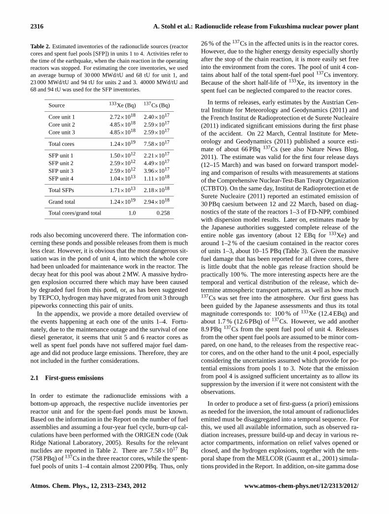
Table 1. Overview of the reactor blocks (units) at the FD-NPP according to Table “Generation Facilities at the Fukushima Dai-ichi NPS”(not numbered, on p. 46) and Table IV-3-1 inNuclear Emergency Response Headquarters(2011).
Unit 1 Unit 2 Unit 3 Unit 4 Unit 5 Unit 6
Electric power output (MW) 460 784 784 784 784 1100Begin commercial operation 1971 1974 1976 1978 1978 1979Reactor model BWR 3 BWR 4 BWR 4 BWR 4 BWR 5 BWR 5Containment type Mark-1 Mark-1 Mark-1 Mark-1 Mark-1 Mark-2Operating/time of shut-down operating operating operating 2010-11-29 2011-01-02 2010-08-13Number of fuel assemblies in core 400 548 548 0 – –Number of fuel assemblies in pond 392 615 566 1535 994 940
eruption in spring 2010 (Stohl et al., 2011a), is closely re-lated to the problem posed by the Fukushima nuclear acci-dent. In both cases we have a point source with unknownvertical and temporal distribution of the emissions. How-ever, while for volcanic ash millions of satellite observationswere made, observations of radionuclides are available onlyas point measurements at certain monitoring sites, and witha coarse temporal resolution of typically 24 h. Even thoughwe have collected measurements from a large set of stationsin Japan and throughout the entire Northern Hemisphere,the total number of available observations is only of the or-der of one thousand. While this makes the problem muchless well conditioned than for the volcanic ash scenario, stillmuch can be learned about the FD-NPP source term by us-ing the top-down inverse method, especially if the inversioncan be guided by a bottom-up a priori (first guess) estimatebased on carefully compiled information. In this paper, wedetermine the emissions of two important radionuclides, thenoble gas xenon-133 (133Xe, lifetime of 5.25 days) and theaerosol-bound caesium-137 (137Cs, lifetime of 30 yr), whichhave very different release and transport characteristics, andfor which measurement data are relatively abundant. We thenuse the model to simulate the atmospheric dispersion and, for137Cs, the deposition over Japan and throughout the NorthernHemisphere.
The paper is structured as follows: In Sect.2, we give anoverview of the accident events that had led to the disasterand how knowledge of these events was used to determinea priori emissions. In Sect.3 we present the measurementdata and model used and describe the inversion method. InSect.4, we report our emission estimates, provide a compar-ison of measured and modeled concentrations and depositionamounts, and present the simulated concentration and depo-sition fields and put them into meteorological context. InSect.5, we draw conclusions from our work.
2 Accident events and first-guess emissions
Fukushima is a prefecture in the East of the Japanese islandHonshu. On its eastern coast, two nuclear power plant com-plexes are located, called Fukushima-I or Fukushima Dai-
ichi, and Fukushima-II or Fukushima Dai-ni1, operated bythe company TEPCO. Fukushima Dai-ichi (FD-NPP), wherethe severe accidents occurred, consists of six boiling waterreactors lined up directly along the shore. The reactor blocksare built in pairs. Table1 gives an overview of the units.When the earthquake occurred, units 4 to 6 had been alreadyshut down for several months for maintenance, while units 1to 3 were under operation at their rated power.
Nuclear reactors also house pools for initial storage ofspent fuel assemblies. In the boiling water reactor (BWR)design, this pool is located outside the containment near thetop of the reactor building. Table1 indicates the amount offuel in these ponds. Even considering that shorter lived nu-clides have decayed, it is obvious that these ponds present asignificant inventory of radioactivity. Furthermore, there is alarger common spent fuel pool at the site, on ground level.Spent fuel is transferred to this pool after at least 19 months,but the decay heat is large enough to still require active cool-ing. This pond contained 6375 fuel assemblies.
The earthquake triggered the automatic shutdown of thechain reaction in the units 1 to 3 at 05:46 UTC (that is 14:46Japan Standard Time) on 11 March. Outside power sup-ply was lost and the emergency diesel generators started up.However, when the tsunami arrived 50 minutes later, it in-undated the sites of the reactors and their auxiliary buildingsand caused the total loss of AC power, except for one of thethree diesel generators of unit 6. Although at different rates,cooling of the reactor cores was lost, water levels in the reac-tor pressure vessels could not be maintained, and in all threeunits that had been under operation, the cores degraded and,as has been reported, partially (or maybe even completely)melted. The hydrogen produced in this process caused ma-jor explosions which massively damaged the upper parts ofthe reactor buildings of units 1 and 3. Damage to the up-per parts of the reactor building could be prevented in unit 2,however, a hydrogen explosion there presumably damagedthe suppression chamber.
Cooling was lost as well for the spent fuel ponds, leadingto heating up of the water and raising concerns about fuel
1ichi means 1, ni means 2
www.atmos-chem-phys.net/12/2313/2012/ Atmos. Chem. Phys., 12, 2313–2343, 2012
2316 A. Stohl et al.: Radionuclide release from Fukushima nuclear power plant
Table 2. Estimated inventories of the radionuclide sources (reactorcores and spent fuel pools [SFP]) in units 1 to 4. Activities refer tothe time of the earthquake, when the chain reaction in the operatingreactors was stopped. For estimating the core inventories, we usedan average burnup of 30 000 MWd/tU and 68 tU for unit 1, and23 000 MWd/tU and 94 tU for units 2 and 3. 40000 MWd/tU and68 and 94 tU was used for the SFP inventories.
Source 133Xe (Bq) 137Cs (Bq)
Core unit 1 2.72×10¹⁸ 2.40×10¹⁷
Core unit 2 4.85×10¹⁸ 2.59×10¹⁷
Core unit 3 4.85×10¹⁸ 2.59×10¹⁷
Total cores 1.24×10¹⁹ 7.58×10¹⁷
SFP unit 1 1.50×10¹² 2.21×10¹⁷
SFP unit 2 2.59×10¹² 4.49×10¹⁷
SFP unit 3 2.59×10¹² 3.96×10¹⁷
SFP unit 4 1.04×10¹³ 1.11×10¹⁸
Total SFPs 1.71×10¹³ 2.18×10¹⁸
Grand total 1.24×10¹⁹ 2.94×10¹⁸
Total cores/grand total 1.0 0.258
rods also becoming uncovererd there. The information con-cerning these ponds and possible releases from them is muchless clear. However, it is obvious that the most dangerous sit-uation was in the pond of unit 4, into which the whole corehad been unloaded for maintenance work in the reactor. Thedecay heat for this pool was about 2 MW. A massive hydro-gen explosion occurred there which may have been causedby degraded fuel from this pond, or, as has been suggestedby TEPCO, hydrogen may have migrated from unit 3 throughpipeworks connecting this pair of units.
In the appendix, we provide a more detailed overview ofthe events happening at each one of the units 1–4. Fortu-nately, due to the maintenance outage and the survival of onediesel generator, it seems that unit 5 and 6 reactor cores aswell as spent fuel ponds have not suffered major fuel dam-age and did not produce large emissions. Therefore, they arenot included in the further considerations.
2.1 First-guess emissions
In order to estimate the radionuclide emissions with abottom-up approach, the respective nuclide inventories perreactor unit and for the spent-fuel ponds must be known.Based on the information in the Report on the number of fuelassemblies and assuming a four-year fuel cycle, burn-up cal-culations have been performed with the ORIGEN code (OakRidge National Laboratory, 2005). Results for the relevantnuclides are reported in Table2. There are 7.58×10¹⁷ Bq(758 PBq) of137Cs in the three reactor cores, while the spent-fuel pools of units 1–4 contain almost 2200 PBq. Thus, only
26 % of the137Cs in the affected units is in the reactor cores.However, due to the higher energy density especially shortlyafter the stop of the chain reaction, it is more easily set freeinto the environment from the cores. The pool of unit 4 con-tains about half of the total spent-fuel pool137Cs inventory.Because of the short half-life of133Xe, its inventory in thespent fuel can be neglected compared to the reactor cores.
In terms of releases, early estimates by the AustrianCen-tral Institute for Meteorology and Geodynamics(2011) andthe FrenchInstitut de Radioprotection et de Surete Nucleaire(2011) indicated significant emissions during the first phaseof the accident. On 22 March,Central Institute for Mete-orology and Geodynamics(2011) published a source esti-mate of about 66 PBq137Cs (see alsoNature News Blog,2011). The estimate was valid for the first four release days(12–15 March) and was based on forward transport model-ing and comparison of results with measurements at stationsof the Comprehensive Nuclear-Test-Ban Treaty Organization(CTBTO). On the same day,Institut de Radioprotection et deSurete Nucleaire(2011) reported an estimated emission of30 PBq caesium between 12 and 22 March, based on diag-nostics of the state of the reactors 1–3 of FD-NPP, combinedwith dispersion model results. Later on, estimates made bythe Japanese authorities suggested complete release of theentire noble gas inventory (about 12 EBq for133Xe) andaround 1–2 % of the caesium contained in the reactor coresof units 1–3, about 10–15 PBq (Table3). Given the massivefuel damage that has been reported for all three cores, thereis little doubt that the noble gas release fraction should bepractically 100 %. The more interesting aspects here are thetemporal and vertical distribution of the release, which de-termine atmospheric transport patterns, as well as how much137Cs was set free into the atmosphere. Our first guess hasbeen guided by the Japanese assessments and thus its totalmagnitude corresponds to: 100 % of133Xe (12.4 EBq) andabout 1.7 % (12.6 PBq) of137Cs. However, we add another8.9 PBq137Cs from the spent fuel pool of unit 4. Releasesfrom the other spent fuel pools are assumed to be minor com-pared, on one hand, to the releases from the respective reac-tor cores, and on the other hand to the unit 4 pool, especiallyconsidering the uncertainties assumed which provide for po-tential emissions from pools 1 to 3. Note that the emissionfrom pool 4 is assigned sufficient uncertainty as to allow itssuppression by the inversion if it were not consistent with theobservations.
In order to produce a set of first-guess (a priori) emissionsas needed for the inversion, the total amount of radionuclidesemitted must be disaggregated into a temporal sequence. Forthis, we used all available information, such as observed ra-diation increases, pressure build-up and decay in various re-actor compartments, information on relief valves opened orclosed, and the hydrogen explosions, together with the tem-poral shape from the MELCOR (Gauntt et al., 2001) simula-tions provided in the Report. In addition, on-site gamma dose
Atmos. Chem. Phys., 12, 2313–2343, 2012 www.atmos-chem-phys.net/12/2313/2012/
A. Stohl et al.: Radionuclide release from Fukushima nuclear power plant 2317
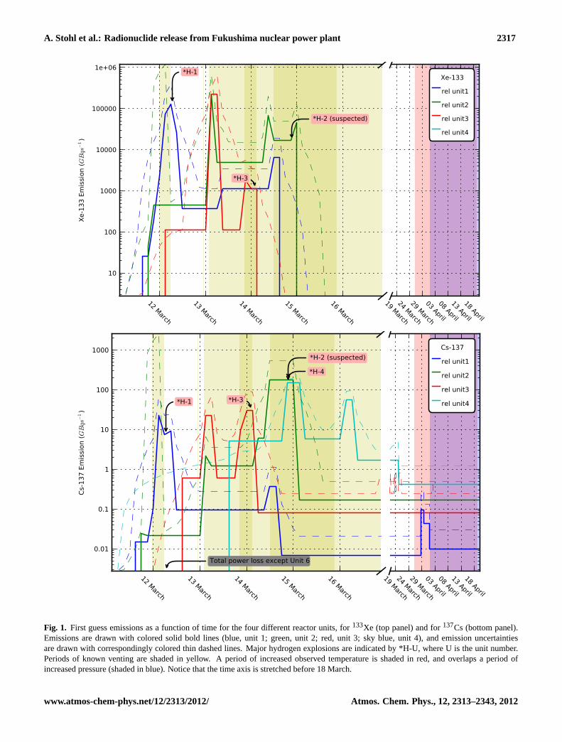
Fig. 1. First guess emissions as a function of time for the four different reactor units, for133Xe (top panel) and for137Cs (bottom panel).Emissions are drawn with colored solid bold lines (blue, unit 1; green, unit 2; red, unit 3; sky blue, unit 4), and emission uncertaintiesare drawn with correspondingly colored thin dashed lines. Major hydrogen explosions are indicated by *H-U, where U is the unit number.Periods of known venting are shaded in yellow. A period of increased observed temperature is shaded in red, and overlaps a period ofincreased pressure (shaded in blue). Notice that the time axis is stretched before 18 March.
www.atmos-chem-phys.net/12/2313/2012/ Atmos. Chem. Phys., 12, 2313–2343, 2012
2318 A. Stohl et al.: Radionuclide release from Fukushima nuclear power plant
rate monitoring data published by TEPCO in their bulletins2
have been used. This latter data source is only a very roughguidance for two reasons. Firstly, the published data refer todifferent locations on the reactor site for different time peri-ods (and published documents do not explain why monitor-ing posts were changed), and secondly, complex interactionbetween wind conditions, release locations and monitoringlocations must be expected but cannot be resolved by us dueto a lack of detailed data.
Figure1 shows the time variation of the derived first-guessemissions and their assumed uncertainties separately for eachreactor unit and relates them to certain events (see the ap-pendix for detailed description). The first guess uncertain-ties are much higher than the emissions, giving the inver-sion enough freedom to change the a priori emissions sub-stantially. Comparing133Xe and137Cs emissions, the133Xeemissions occur over much shorter periods of time, as mostof the noble gas inventory is assumed to be injected into theatmosphere by the first venting event at each unit. Emissionsof 137Cs are more influenced by the hydrogen explosions andgenerally occur over a more extended time period, while onlya small part of the inventory is released.
For the inversion, it is not possible to consider the emis-sions for each unit separately and, thus, all emissions weresummed. Uncertainties are probably not strictly additive, butwere also summed. The emissions from spent-fuel pools andreactor cores could in principle be disentangled using nuclideratios or joint inversions of several nuclides, but this is out ofthe scope of this paper. However, in the interpretation of theresults, we will try to partly relate changes of the emissionsto certain events at individual reactor units. All in all, theresulting first guess is obviously a largely subjective productwith major uncertainty margins.
2.2 Release heights
Atmospheric transport of emitted nuclides depends on theheight of the source, due to vertical wind shear and also tur-bulence conditions. Considering that the present problem israther weakly constrained, releases are divided into three lay-ers only: 0–50 m, 50–300 m, and 300–1000 m above groundlevel. The a priori source term needs to be divided betweenthese three layers. The height of the reactor buildings of FD-NPP is 40 m, so any leakages through wall or roof openingswould fall into the first emission layer. Then, each pair ofunits has an exhaust stack which emits into the second layer.Some of the venting may have occurred through these stacks.Also, the effluents are hot and thus there can be thermalplume rise, contributing to emissions into the second layer.The third layer is thought to be involved only for the pe-riod of explosions. Thus, the initial releases were divided
2kindly made available in a consistent spreadsheet by M. Taki-gawa from the Japan Agency for Marine-Earth Science and Tech-nology
between first and second layer in a ratio 70:30, then in thoseunits where explosions occurred, after the explosion the ra-tio was set to 50:50. During the explosion in unit 1, 20 %were assumed to be emitted into the third layer. The unit 2explosion did not produce building damage and is not consid-ered to have increased the effective release height. The unit3 explosion was much more powerful, and movies show thatmaterial is ejected high up into the atmosphere, thus 70 %of the emissions were placed into the third layer for the cor-responding 3 h interval. As for the unit 4 explosion, it wasassumed that 10 % went into the third layer.
3 Methods
3.1 Measurement data
We collected measurements of atmospheric activity concen-trations from a variety of sources, as listed in Tables4 and5,which also report the total number of samples available foreach station during the period of our study. Measurementsof atmospheric activity concentrations of both133Xe and137Cs were available from CTBTO stations. The Compre-hensive Nuclear-Test-Ban Treaty (CTBT) foresees a globalban of all nuclear explosions. To verify compliance with theCTBT, a global international monitoring system with fourdifferent measurement technologies is currently being builtup, namely for seismic (170 stations), hydroacoustic (11 sta-tions), infrasound (60 stations) and radionuclide (80 stations)monitoring (Hoffmann et al., 2000). As far as the radionu-clide monitoring subsystem is concerned, 60 particulate mat-ter monitoring stations are currently delivering data to theInternational Data Centre of the Preparatory Commission forthe CTBTO in Vienna. The stations are all equipped withhigh-volume aerosol samplers. About 20 000 m3 of air isblown through a filter, collecting particulate radionuclides.Gases are not retained in the filters. The collection pe-riod is 24 h. The different radionuclides are measured withhigh-resolution germanium detectors (Schulze et al., 2000;Medici, 2001). The minimum detectable activity concentra-tion of 137Cs is 1 µBq m−3, which is about three orders ofmagnitude lower than for measurements within typical na-tional radiation monitoring networks.
As part of CTBT treaty monitoring, half of the radionu-clide stations shall additionally be equipped with xenon de-tectors. During the International Noble Gas Experiment(INGE), noble gas measurement systems have been set upworldwide (Wernsberger and Schlosser, 2004; Saey and deGeer, 2005). Currently, about 25 stations are delivering datato CTBTO. The radioxenon isotopes measured are131mXe,133mXe, 133Xe and135Xe, with half-lives of 11.93 days, 2.19days, 5.25 days and 9.14 h, respectively. The most prevalentand important isotope is133Xe, which is measured with anaccuracy of about 0.1 mBq m−3. The typical global distribu-tion of this isotope is described byWotawa et al.(2010). The
Atmos. Chem. Phys., 12, 2313–2343, 2012 www.atmos-chem-phys.net/12/2313/2012/
A. Stohl et al.: Radionuclide release from Fukushima nuclear power plant 2319
Table 3. Release fractions and estimated released activities from various sources, including the first guess (FG) estimate used in this workand our best a posteriori estimate. “Report Att. IV-2” refers to MELCOR (Gauntt et al., 2001) simulation results as reported in Table 5 ofAttachment IV-2 of the Report. ZAMG refers to the estimate byCentral Institute for Meteorology and Geodynamics(2011) for the first fourdays of the event. ISRN lists the estimate ofInstitut de Radioprotection et de Surete Nucleaire(2011) for 12–22 March 2011.
Source 133Xe ( %) 133Xe (EBq) 137Cs ( %) 137Cs (PBq)
Report Att. IV-2 97.3 12.2 1.7 16.4Report Att. VI 97.3 12.2 0.8 7.5SPEEDI (Att. VI-1) – – 1.4 13.0ZAMG – – – 66.0ISRN – – – 30.0
FG core 1 100 2.7 0.3 0.7FG core 2 100 4.8 4.0 10.4FG core 3 100 4.8 0.6 1.6
FG cores 1–3 100 12.4 1.7 12.6FG SFP 4 – – 0.8 8.9
FG total 100 12.4 1.2 21.5A posteriori 100 15.3 2.0 36.6
Table 4. List of stations used for the133Xe inversions, sorted by longitude. Num gives the number of valid observations used for theinversion.
Station name Longitude Latitude Num Data source
Wake Island 166.6 19.3 40 CTBTOOahu −158.0 21.5 79 CTBTOSidney −123.4 48.7 38 I. Hoffman, personal
communication (2011)Richland −119.3 46.3 72 Bowyer et al. (2011)Yellowknife −114.5 62.5 33 CTBTOAshland −99.8 37.2 79 CTBTOPanama City −79.5 9.0 14 CTBTOCharlottesville −78.4 38.0 76 CTBTOOttawa −75.7 45.4 27 CTBTOSt. John’s −52.7 47.6 38 CTBTOSchauinsland 7.9 47.9 39 CTBTOSpitsbergen 15.4 78.2 79 CTBTOStockholm 17.6 59.2 79 CTBTOUlan-Bator 106.3 47.9 37 CTBTOGuangzhou 113.3 23.0 39 CTBTODarwin 130.9 −12.4 78 CTBTOUssuriysk 132.0 44.2 59 CTBTO
Total 906
collection period of the xenon samples is typically 12 h. Allmeasured radionuclide concentrations were decay-correctedfor the sampling period to the end of the sampling intervaland converted from activity per norm cubic meter at standardtemperature and pressure (273.15 K and 101 325 Pa) to activ-ity per cubic meter (using meteorological analysis data) forcomparison with the model results. For the purpose of in-verse modeling, the data were further decay-corrected to thetime of the earthquake.
Two stations of the CTBTO network, Okinawa andTakasaki, are located in Japan, but133Xe measurements aremade only at Takasaki. However, the Takasaki noble gas de-tections were, for an extended period of time, reaching thedynamic range of the system, meaning that measurementswere so high that they became unreliable. In addition to that,there were also considerable memory effects. While someresearchers (K. Ungar, personal communication, 2011) havemade attempts to extract quantitative information from these
www.atmos-chem-phys.net/12/2313/2012/ Atmos. Chem. Phys., 12, 2313–2343, 2012

2320 A. Stohl et al.: Radionuclide release from Fukushima nuclear power plant
Table 5. List of stations used for the137Cs inversions, sorted by longitude. Num gives the number of valid observations used for theinversion. NIES is the National Institute for Environmental Studies, JCAC is the Japan Chemical Analysis Center, JAEA is the Japan AtomicEnergy Agency with data points fromFuruta et al.(2011).
Station name Longitude Latitude Num Data source
Nankang 121.6 23.5 23 Hsu et al.(2012)Pengchiayu 122.1 25.6 23 Hsu et al.(2012)Okinawa 127.9 26.5 39 CTBTOTakasaki 139.0 36.3 38 CTBTOWako 139.6 35.8 31 RIKENTsukuba 140.1 36.0 24 NIESChiba 140.1 35.7 37 JCACTokai−mura 140.6 36.4 69 JAEA S. Furuta, personal
communication (2011)Guam 144.9 13.6 36 CTBTONew Hanover 150.8 −2.6 36 CTBTOPetropavlovsk 158.8 53.0 40 CTBTOWake Island 166.6 19.3 36 CTBTOMidway Islan −177.4 28.2 39 CTBTOSand Point −160.5 55.3 37 CTBTOOahu −158.0 21.5 39 CTBTOSalchaket −147.1 64.7 39 CTBTOVancouver −123.2 49.2 39 CTBTOSacramento −121.4 38.7 39 CTBTOYellowknife −114.5 62.5 39 CTBTOAshland −99.8 37.2 38 CTBTOResolute −94.9 74.7 37 CTBTOMelbourne −80.6 28.2 39 CTBTOPanama City −79.5 9.0 39 CTBTOCharlottesville −78.4 38.0 39 CTBTOOttawa −75.7 45.4 9 I. Hoffman, personal
communication (2011)St. John’s −52.7 47.6 39 CTBTOIceland −21.9 64.1 13 Ro5Reykjavik −21.8 64.1 38 CTBTOCaceres −6.3 39.5 16 Ro5Orsay 2.2 48.7 19 Ro5Sola 5.7 58.9 23 Ro5Schauinsland 7.9 47.9 27 CTBTOBraunschweig 10.5 53.3 19 Ro5Osteras 10.6 59.9 22 Ro5Spitsbergen 15.4 78.2 31 CTBTOLongyearbyen 15.6 78.2 15 Ro5Stockholm 17.6 59.2 39 CTBTOSvanhovd 30.0 69.4 20 Ro5Dubna 37.3 56.7 39 CTBTOKuwait City 47.9 29.3 39 CTBTOKirov 49.4 58.6 36 CTBTOZalesovo 84.8 53.9 39 CTBTOUlan−Bator 106.3 47.9 39 CTBTOQuezon City 121.4 14.6 39 CTBTOUssuriysk 132.0 44.2 38 CTBTO
Total 1494
Atmos. Chem. Phys., 12, 2313–2343, 2012 www.atmos-chem-phys.net/12/2313/2012/

A. Stohl et al.: Radionuclide release from Fukushima nuclear power plant 2321
data, we decided to not use133Xe data from Takasaki for ourinversions.
Regarding the137Cs measurements at Takasaki, there wasanother problem. During the first passage of the plume atthis station, radioactivity entered the interior of the build-ing. This resulted in a serious contamination, meaning that137Cs shows up continuously in the measurements since theinitial event, even when it is probably completely absentin the ambient air. We applied a correction of the data(seehttp://www.cpdnp.jp/pdf/110818Takasakireport revise.pdf, downloaded on 16 August). Still, the contamination isa potential problem for the inversion, which may attempt toattribute the erroneously measured activity to direct releasesfrom FD-NPP. Similar features can be noticed also in the datafrom the other Japanese stations. This might partly also becaused by contamination problems but we are lacking de-tailed information. In addition, resuspension either from thesurroundings or from heavily contaminated areas elsewhere,is possible as well. In fact, such resuspension is necessaryto explain the relatively more rapid decay of radiation doserates in highly contaminated areas than in less contaminatedareas (Yamauchi, 2012).
When using the CTBTO data, we found that these dataalone could not provide sufficient constraints on the emis-sions (see also Sect.4.1). This is true especially for137Cs, forwhich the modeled concentrations far from Japan are highlysensitive to changes in the modeling of wet scavenging andthus the model uncertainties are large. We therefore addedseveral non-CTBTO data sets. Measurements of137Cs atfour Japanese stations were started only on 14–15 Marchwhen the accident at FD-NPP was already in full progress.For the first few weeks, the data collection followed irregularschedules, as attempts were made to take frequent measure-ments during plume passages. Some of the samples werecollected over less than one hour, whereas some of the latersamples were collected over several days.
We also added data from a few non-CTBTO stations out-side Japan, two measuring133Xe and eleven measuring137Cs(see Tables4 and5). These stations were selected becausethey documented plume passages very well and offered gooddata quality. In particular, measurement data from a sub-setof the European network ”Ring of five” (Ro5) were used.Measurements of this network following the FD-NPP acci-dent were described byMasson et al.(2011). Measurementsof 137Cs from two stations in Taiwan were described byHsuet al.(2012) and provided by these authors.133Xe measure-ments made at Richland were described byBowyer et al.(2011) and were kindly made available (H. Miley, personalcommunication, 2011).133Xe measurements made at Sidney(Canada) were kindly provided by K. Ungar and I. Hoffman(personal communication, 2011).
Measurements of137Cs deposition (”fallout”) were per-formed by MEXT at 46 sites in all of Japan’s 47 prefecturesexcept Miyagi. The coordinates of these sites are confiden-tial but were made available to us. Daily measurements using
bulk samplers started on 18 March and a total of 1497 24-hsamples were available for the period of our study. Thesedata were quality-checked and updated for an earlier pub-lication (Yasunari et al., 2011). Later revisions of a fewdata points by MEXT were taken into account. Furthermore,12 deposition measurements were available from Tokai-murawith an irregular time resolution following rain events. Dif-ferent deposition samplers were used at the various sites and,for the inverse modeling, it was assumed that the measureddeposition is a result of both dry and wet deposition, eventhough dry deposition onto these samplers may not be repre-sentatitve for dry deposition onto the surrounding landscape.
The inversion needs information on the uncertainties as-sociated with each observation value. For most data sets(all CTBTO data, plus some others), measurement uncer-tainties were available and used. Where such informationwas not available, we assumed a relative uncertainty of 5 %for the concentration data and 10 % for the deposition dataand added absolute uncertainties of 0.2 mBq m−3 for 133Xeconcentration data, 1 µBq m−3 for 137Cs concentration data,and 2 Bq m−2 for 137Cs deposition data. Furthermore, to ad-dress the problem of137Cs contamination and resuspensionat Japanese stations, we used 1 per mille of the highest pre-viously measured137Cs concentration (or deposition) at agiven station as the minimum observation uncertainty, un-less the measured concentration (deposition) was below thatthreshold.
3.2 Model simulations
To simulate radionuclide dispersion, we used the Lagrangianparticle dispersion model FLEXPART (Stohl et al., 1998;Stohl and Thomson, 1999; Stohl et al., 2005). This modelwas originally developed for calculating the dispersion of ra-dioactive material from nuclear emergencies but has sincebeen used for many other applications as well. Nuclear appli-cations include, for instance, simulations of the transport ofradioactive material from NPPs and other facilities (Andreevet al., 1998; Wotawa et al., 2010) or from nuclear bomb tests(Becker et al., 2010). FLEXPART is also the model oper-ationally used at CTBTO for atmospheric backtracking andat the Austrian Central Institute for Meteorology and Geody-namics for emergency response as well as CTBT verificationpurposes.
For this study, FLEXPART was driven with three-hourlyoperational meteorological data from two different sources,namely the European Centre for Medium-Range WeatherForecasts (ECMWF) analyses, and the National Centers forEnvironmental Prediction (NCEP) Global Forecast System(GFS) analyses. The ECMWF data had 91 model levels anda resolution of 0.18◦×0.18◦ in the region 126◦–180◦ E and27◦–63◦ N and 1◦×1◦ elsewhere, and the GFS data had 26model levels and a resolution of 0.5◦
×0.5◦ globally. Bothdata sets do not resolve the complex topography of Japanvery well, but in the simulations air masses from FD-NPP
www.atmos-chem-phys.net/12/2313/2012/ Atmos. Chem. Phys., 12, 2313–2343, 2012
2322 A. Stohl et al.: Radionuclide release from Fukushima nuclear power plant
were blocked by the mountain chains from directly reach-ing western Honshu Island, where radionuclide measurementdata indeed showed no direct impact of FD-NPP emissions.
To improve the a priori emissions by the inversion algo-rithm, it was necessary to run the dispersion model forwardin time for each one of the 972 (3 layers×324 3-h inter-vals between 12:00 UTC on 10 March and 00:00 UTC on 20April) emission array elements. Each one of these 972 sim-ulations quantified the sensitivity of downwind atmosphericactivity concentrations and depositions to the emissions in asingle time-height emission array element. The simulationsextended from the time of emission to 20 April 00:00 UTCand carried one million particles each. A total of about 1 bil-lion particles was used. Per simulation, unit masses of twotracers were released: firstly, a passive noble gas tracer and,secondly, an aerosol tracer that was subject to wet and drydeposition. Radioactive decay was not included in the modelsimulations, since all radionuclide observations and also thea priori emission data were corrected to the time of the earth-quake for the purpose of the inverse modeling.
For the aerosol tracer, the simulations accounted forwet and dry deposition, assuming a particle density of1900 kg m−3 and a logarithmic size distribution with an aero-dynamic mean diameter of 0.4 µm and a logarithmic stan-dard deviation of 0.3. The wet deposition scheme considersbelow-cloud and within-cloud scavenging separately, assum-ing clouds are present where the relative humidity exceeds80 %. Within-cloud scavenging coefficients are calculated asdescribed inHertel et al.(1995) and below-cloud scaveng-ing coefficients are based onMcMahon and Denison(1979),allowing also for sub-grid variability of precipitation rate.The wet deposition scheme is documented in the FLEXPARTuser manual available fromhttp://transport.nilu.no/flexpart.Tests showed large sensitivity of simulated137Cs concentra-tions to the in-cloud scavenging coefficient. We exploredthis sensitivity by performing model simulations where allscavenging coefficients were scaled to 67 and 150 % of theirnormal values. These sensitivity simulations, along with thereference simulation, were used as part of the ensemble forquantifying the model error needed by the inversion.
The agreement of model results (both using a priori and aposteriori emissions) with measurement data was better withGFS data than with ECMWF data. The fact that this wasalso found for133Xe which is not affected by wet scaveng-ing, shows that GFS-FLEXPART captured the general trans-port better than ECMWF-FLEXPART. Furthermore, the wetscavenging of137Cs was much stronger with ECMWF datathan with the GFS data, causing a strong underestimation of137Cs concentrations at sites in North America and Europe(see Sect.4.4.1). Therefore, all results presented in this pa-per were produced using the GFS data as the reference dataset. The ECMWF-based simulations are, however, used asensemble members in the inversion to quantify the model un-certainties.
3.3 Inversion algorithm
In previous studies, we have developed an inversion algo-rithm to calculate the emissions of greenhouse gases (Stohlet al., 2009) or volcanic sulfur dioxide and ash emissions(Eckhardt et al., 2008; Kristiansen et al., 2010; Stohl et al.,2011a) based on original work bySeibert(2000). Dependingon the application, the algorithm incorporates different typesof observation data and can be based on forward or back-ward calculations with FLEXPART. A full description of thealgorithm was given previously (Eckhardt et al., 2008; Stohlet al., 2009; Seibert et al., 2011) and, therefore, we provideonly a short summary here. Our inversion setup is almostidentical to that described byStohl et al.(2011a), where vol-canic ash emissions were derived as a function of time andaltitude. The only further development is the use of ensem-ble model simulations to quantify the model uncertainty, de-scribed at the end of this section.
We want to determine radionuclide emissions as a func-tion of time (324 3-hourly intervals between 10 March12:00 UTC and 20 April 00:00 UTC) and altitude (three lev-els: 0–50 m, 50–300 m, 300–1000 m), yielding a total ofn = 972 unknowns denoted as vectorx. For each one of then unknowns, a unit amount of radionuclide was emitted inFLEXPART and the model results (surface concentrationsor deposition values) were matched (i.e., ensuring spatio-temporal co-location) withm radionuclide observations (seeSect.3.1) put into a vectoryo. Modeled valuesy correspond-ing to the observations can be calculated as
y = Mx (1)
whereM is them×n matrix of source-receptor relationshipscalculated with FLEXPART.
As the problem is ill-conditioned with the measurementdata not giving a strong constraint on all elements of thesource vector, regularization or, in other words, additionala priori information is necessary to obtain a meaningful so-lution. Including the a priori source vectorxa , we can write
M(x −xa) ≈ yo−Mxa (2)
and as an abbreviation
Mx ≈ y. (3)
Considering only the diagonals of the error covariance ma-trices (i.e., only standard deviations of the errors while as-suming them to be uncorrelated), the cost function to be min-imized is
J = (Mx − y)T diag(σo−2) (Mx − y)+ xT diag(σx
−2) x
+(Dx)T diag(ε) Dx. (4)
The first term on the right hand side of Eq. (4) measures themisfit model–observation, the second term measures the de-viation from the a priori values, and the third term measuresthe deviation from smoothness.σo is the vector of standard
Atmos. Chem. Phys., 12, 2313–2343, 2012 www.atmos-chem-phys.net/12/2313/2012/
A. Stohl et al.: Radionuclide release from Fukushima nuclear power plant 2323
errors of the observations, andσx the vector of standard er-rors of the a priori values. The operatordiag(a) yields adiagonal matrix with the elements ofa in the diagonal.Dis a matrix with elements equal to−2 or 1 giving a discreterepresentation of the second derivative, andε is a regulari-sation parameter determining the weight of this smoothnessconstraint compared to the other two terms.
The above formulation implies normally distributed, un-correlated errors, a condition that we know to be not ful-filled. Observation errors (also model errors are subsumedin this term) may be correlated with neighboring values, anddeviations from the prior sources are likely to be asymmet-ric, with overestimation being more likely than underesti-mation as zero is a natural bound. The justification for us-ing this approach is the usual one: the problem becomesmuch easier to solve, detailed error statistics are unknownanyway, and experience shows that reasonable results can beobtained. Negative emission values can occur in this set-upbut were removed in an iterative procedure by binding themmore strongly to the positive a priori values.
Two important changes to the algorithm were made sinceour last application (Stohl et al., 2011a). The first changewas required because the current problem is data-sparse andsome individual emission values are not well constrained bythe measurement data. This ill-conditioning was also en-countered byDavoine and Bocquet(2007) in their inversemodel study of the Chernobyl source term. For the volcanicash problem, we used more than two million satellite obser-vations (Stohl et al., 2011a), whereas here only of the orderof one thousand observations were available. Partly this wascompensated by reducing the number of vertical levels forwhich emissions were determined from 19 to 3. Due to thispoor vertical resolution, we removed the vertical smoothnesscondition used byStohl et al.(2011a) and instead imposeda variable temporal smoothing condition. This was simplyachieved by restructuringD and ε. The smoothing servesas an additional a priori constraint, which favors correctionsof the a priori emissions that do not vary strongly with time.This stabilizes the inversion and reduces the noise level in thesolution. Since there were a number of known incidents atFD-NPP when emission rates are suspected to have changedrapidly, we use a variable smoothness parameterε. Weaksmoothing was imposed when the a priori emissions changedrapidly, while stronger smoothing was imposed during peri-ods with no reported events.
A second change was made to improve the representationof model error in the inversion. As described in Sect.3.2, anensemble of FLEXPART calculations was made using twometeorological data sets and changing the magnitude of thewet scavenging coefficients for137Cs to quantify the twomost important sources of model error related to the me-teorological input data and the wet scavenging parameters.The source-receptor relationships for all these model simula-tions were read into the inversion algorithm simultaneouslyto evaluate a range of a priori modeled concentration and de-
position values. Their standard error was used as a proxy forthe model error. Model and measurement error were com-bined into the observation errorσo =
√σ 2
meas+σ 2mod, where
σmeasis the measurement error andσmod the model error.While the inversion method formally propagates stochas-
tic errors in the input data into an a posteriori emission un-certainty, the overall error is determined also by partly sys-tematic other errors. For instance, the inversion assumes nor-mally distributed errors, which is not the case. The inversionalso treats all emission values and all observations as inde-pendent from each other, which is also not the case. How-ever, lacking detailed error statistics, this cannot be formallyaccounted for. These additional errors can to some extent beexplored with sensitivity experiments (see section4.2.3).
For 137Cs, we have used measurements of both atmo-spheric activity concentrations as well as deposition to con-strain the source term. It was already mentioned byGudik-sen et al.(1989) that it is preferable to use concentrationmeasurements for inverse modeling because of the additionaluncertainties related to modeling the deposition process, in-cluding the correct capture of location and time of precipita-tion events. However, in a data-sparse situation all availabledata should be used. There are 1497 Japanese depositionmeasurements available, while only 238 of the 1494 con-centration measurements were made in Japan. By varyingthe wet scavenging parameters and the meteorological inputdata of our dispersion model, the uncertainties of the mod-eled deposition values are reasonably well quantified, so thatthe deposition data can provide valuable information. Fur-thermore, errors in modeling the deposition process will af-fect atmospheric concentrations and deposition values in theopposite way. Thus, combining these two types of data willpartly lead to error compensation in the inverse modeling.
4 Results
4.1 Sensitivity of the station network to emissions fromFD-NPP
Determining the emissions from FD-NPP is a data-poorproblem and it is important to first explore to what extentthe measurement data can actually provide constraints onthe emissions. Figure2 shows the total sensitivity of themeasurement network to133Xe emissions, i.e., the emissionsensitivities (source-receptor relationships) summed over allm observation cases. This provides important informa-tion on the minimum source strength detectable by the sta-tion network. For the minimum detection threshold for aCTBTO station of 1 mBq m−3, an emission sensitivity of1×10−11 Bq m−3 per Bq s−1 means that a 3-h-long emissionpulse larger than 1×10⁸ Bq s−1 is detectable. The largest ex-pected emission rates are of the order of 1014 Bq s−1, six or-ders of magnitude larger.
www.atmos-chem-phys.net/12/2313/2012/ Atmos. Chem. Phys., 12, 2313–2343, 2012

2324 A. Stohl et al.: Radionuclide release from Fukushima nuclear power plant
1e-012
1e-011
0310 0317 0324 0331 0407 0414
Sen
sitiv
ity (
Bq/
m3
per
Bq/
s)
Date
Layer 1Layer 2Layer 3
Fig. 2. Sensitivity of the station network to133Xe emissions at FD-NPP. The sensitivities are calculated separately for emissions at thelowest layer (0–50 m, red), middle layer (50–300 m, black) and toplayer (300–1000 m, blue).
The modeled emission sensitivity for March 2011 variesby about one order of magnitude and drops rapidly on 7 April2011. The reason for the rapid decrease is that releases after7 April had little chance to be sampled before 20 April bythe 133Xe measurement network consisting only of stationsfar from Japan (see Table4). However, as we shall see later,this does not affect our capability to quantify the emissionsfrom FD-NPP, since the entire inventory of133Xe was setfree into the atmosphere before 16 March.
The accumulated emission sensitivities for the three emis-sion layers are very similar most of the time (Fig.2), sug-gesting similarity of transport. While differences can belarger when considering individual measurement samplesseparately, the overall similarity indicates that the inversionmay not always be able to clearly distinguish the emissionsfrom the three height layers.
To determine137Cs emissions, we used both air concen-tration as well as deposition data and we therefore con-sider the emission sensitivity for both data types separately(Fig. 3). In contrast to133Xe, the emission sensitivity for137Cs varies by several orders of magnitude, both for theconcentration and deposition data. Periods for which airfrom FD-NPP was sampled directly by the Japanese stationsare characterized by high sensitivity, in contrast to periodswhen air from FD-NPP was transported to the Pacific Oceanand could be sampled only by remote stations. Removalof 137Cs by precipitation scavenging adds more variability.Considering a minimum detectable137Cs concentration of1 µBq m−3, an emission sensitivity of 1×10⁻¹⁵ Bq m−3 perBq s−1 (i.e., the lowest sensitivity before 12 April) allowsdetection of an emission of 1×10⁹ Bq s−1, about two ordersof magnitude less than the highest expected emission rates.For the deposition measurements, sensitivities vary betweenabout 1×10⁻¹² Bq m−2 per Bq s−1 and 1×10⁻⁶ Bq m−2 perBq s−1. With an optimistic detection threshold of 2 Bq m−2,emissions larger than 5×10⁶ Bq s−1 to 5×10¹² Bq s−1 can be
detected. This means that the deposition measurements aloneconstrain the source term only for certain periods when theFD-NPP plume passed directly over Japan.
Overall, we see that133Xe emissions of “expected” magni-tude can be reliably detected by the observations throughoutMarch, while this may not always be the case for137Cs emis-sions below “expected” peak values. Quantification of137Csemissions is made even more difficult by the relatively largemodel errors (see section4.3).
4.2 Emissions
Emission values reported in this section are corrected forradioactive decay to a reference time of 05:46 UTC on 11March 2011, the time of the earthquake. Actual emissionsare lower, especially for the short-lived133Xe.
4.2.1 Xenon-133
Total a posteriori133Xe emissions obtained by the inversionare 15.3±3.1 EBq (uncertainty range will be discussed later),23 % more than the a priori value of 12.4 EBq (which isequal to the estimated inventory) and more than twice theestimated Chernobyl source term of 6.5 EBq (NEA, 2002).This value is in good agreement with independent results(Stohl et al., 2012) which we have obtained by using an atmo-spheric multi-box model (16.7±1.9 EBq) as well as by com-paring FLEXPART model calculations with CTBTO mea-surements of133Xe during the period 11 April to 25 May2011 (14.2±0.8 EBq and 19.0±3.4 EBq when using GFSand ECMWF meteorological input data, respectively). Allvalues obtained are higher than the calculated133Xe inven-tory, which confirms the full release of the noble gas inven-tory of FD-NPP. However, as emissions cannot exceed 100 %of the inventory, there must have been an additional sourceof 133Xe, which presumably is the decay of iodine-133 (133I,half-life 20.8 h) into133Xe as this additional source. Accord-ing to our ORIGEN calculations, the inventories of133Xe and133I were almost identical at the time of the accident. Sincethe half-lives of mother and daughter nuclide have a ratioof approximately 1:6, the additional133Xe activity (decay-corrected to the time of the earthquake) generated by thedecay of133I is about 16.5 % of the original133Xe activity.Thus, the combined133I and133Xe inventories correspond toa total effective133Xe activity of 14.4 EBq, only 0.9 EBq lessthan the value for our a posteriori133Xe release but within itsestimated uncertainty. Most of the133I would have decayedto 133Xe before the first venting at each unit was made andwould have been released together with the originally present133Xe. Smaller amounts of133Xe produced later would stillhave been released as the damaged reactors would not haveconstituted a barrier to noble gas releases. Finally, smallamounts of133Xe can be expected from the decay of133Ithat was released into the environment.
Atmos. Chem. Phys., 12, 2313–2343, 2012 www.atmos-chem-phys.net/12/2313/2012/

A. Stohl et al.: Radionuclide release from Fukushima nuclear power plant 2325
1e-016
1e-015
1e-014
1e-013
1e-012
1e-011
1e-010
1e-009
1e-008
0310 0317 0324 0331 0407 0414
Sen
sitiv
ity (
Bq/
m3
per
Bq/
s)
1e-016
1e-014
1e-012
1e-010
1e-008
1e-006
0310 0317 0324 0331 0407 0414
Sen
sitiv
ity (
Bq/
m2
per
Bq/
s)
Date
layer 1layer 2layer 3
Fig. 3. Sensitivity of the station network to137Cs emissions at FD-NPP, for the atmospheric concentration measurements (upper panel) andfor the deposition measurements (lower panel). The sensitivities are calculated separately for emissions at the lowest layer (0–50 m, red),middle layer (50–300 m, black) and top layer (300–1000 m, blue).
10
100
1000
10000
100000
0310 0311 0312 0313 0314 0315 0316 0317 0318 0
20
40
60
80
100
Em
issi
on (
GB
q/s)
Em
issi
on d
ist.,
a p
riori
(%)a priori
a posteriori
10
100
1000
10000
100000
0310 0311 0312 0313 0314 0315 0316 0317 0318 0
20
40
60
80
100
Em
issi
on U
ncer
tain
ty (
GB
q/s)
Em
issi
on d
ist.,
a p
ost.
(%)
Date
a prioria posteriori
Fig. 4. Emissions of133Xe used a priori (red line) and obtained a posteriori by the inversion (blue line) (upper panel), as well as associateduncertainties (lower panel). The vertical distribution of the emissions over the three layers, with scale on the right hand side, is shown by thebackground colors (0-50 m, light yellow; 50-300 m; light turquoise, 300-1000 m, light red) for the a priori emissions (upper panel) and the aposteriori emissions (lower panel). The orange vertical line indicates the time of the earthquake, and the green vertical lines mark the timeswhen the first venting operations are reported. The data shown in this plot are available as Supplement.
The time variation of a priori and a posteriori emissionsis generally quite consistent (Fig.4), both suggesting thatthe entire133Xe inventory was released between 11 and 15March 2011. However, the a posteriori emissions start 6 hearlier and end 12 h later than our first guess estimate. This
is a robust feature of the inversion, which was obtained alsowith reduced smoothness, increased a priori uncertainty andfor both meteorological data sets. While errors in the tim-ing of emissions are possible with our inversion method,they should be smaller than the 18 h between the time of the
www.atmos-chem-phys.net/12/2313/2012/ Atmos. Chem. Phys., 12, 2313–2343, 2012
2326 A. Stohl et al.: Radionuclide release from Fukushima nuclear power plant
1
10
100
0310 0317 0324 0331 0407 0414 0
20
40
60
80
100
Em
issi
on (
GB
q/s)
Em
issi
on d
ist.,
a p
riori
(%)a priori
a posteriori
1
10
100
0310 0317 0324 0331 0407 0414 0
20
40
60
80
100
Em
issi
on U
ncer
tain
ty (
GB
q/s)
Em
issi
on d
ist.,
a p
ost.
(%)
Date
a prioria posteriori
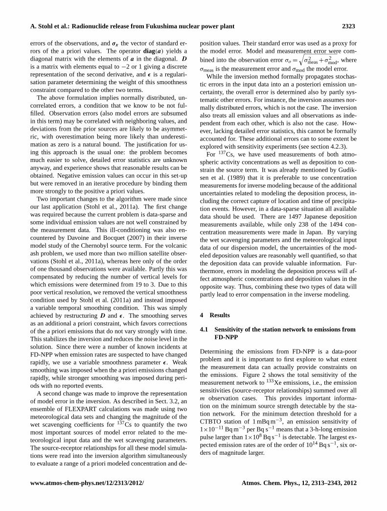
Fig. 5. Emissions of137Cs used a priori (red line) and obtained a posteriori by the inversion (blue line) (upper panel), as well as associateduncertainties (lower panel). The vertical distribution of the emissions over the three layers, with scale on the right hand side, is shown by thebackground colors (0–50 m, light yellow; 50-300 m; light turquoise, 300-1000 m, light red) for the a priori emissions (upper panel) and thea posteriori emissions (lower panel). The orange vertical line indicates the time of the earthquake. The data shown in this plot are availableas Supplement.
earthquake (and also the start of our a posteriori emissions)and the reported time of the first successful venting. Theearly start of a posteriori emissions could be due to a noblegas release as a consequence of the emergency shutdown ofthe reactors, possibly enhanced by structural damage fromthe earthquake and/or leaks due to overpressure. Also theinjection of cold water through the emergency core cool-ing systems and associated thermal stress on fuel claddingsmay contribute to this release. Finally, workers temporar-ily opened an air lock in the reactor building and closed itonly after they observed a white “cloud” coming out. Thus,some radioactivity seems to have leaked out already beforethe pressure relieve valves were opened in reactor unit 1 at00:15 on 12 March, according to the Report. Notice, how-ever, that the retrieved emissions during the first six hoursafter the earthquake are not very large. Large emissions areretrieved from 12:00 UTC on 11 March, the suspected timeof failure of the primary containment vessel, according tothe Report. For a detailed discussion of this early start of theemissions, we refer toStohl et al.(2011b).
The emission peaks on 12, 13, and 14 March are associ-ated with venting events at units 1, 3 and 2, respectively. Itis interesting to notice that in all three cases our a posterioriemissions start increasing earlier than our first guess emis-sions and drop more strongly at the end of the venting. Thisseems to indicate that contaminated air was leaking from thecontainment as pressure was building up, even before activeventing started.
In our first guess,133Xe emissions end after a final peakpresumably caused by a hydrogen explosion which damagedthe wet well of unit 2 at 21:00 UTC on 14 March. Our aposteriori emissions, however, continue until 12:00 UTC on15 March. The pressure vessel and dry well of unit 2 werereported to be at ambient pressure only at 21:00 UTC on 15March, and various valve operations are reported for unit 3until 20 March. This could explain ongoing emissions atleast until 15 March, especially if we consider that the coredegradation may still have been in progress. The inversionresults show no emissions after 15:00 UTC on 15 March.Partly, this may be related to the decreasing emission sen-sitivity at that time (see Fig.2), which also leads to rathersmall reductions in the emission uncertainty after 15 March(lower panel of Fig.4). Therefore, we cannot rule out thepossibility that minor emissions have persisted even after 15March, but they would only constitute a small fraction of thetotal emission.
Regarding the vertical emission distribution, the inversionattributes a larger fraction to layer 2 (50–300 m) than the firstguess, probably indicating that thermal plume rise was oftenimportant (Fig.4, lower panel). However, the vertical attri-bution is very noisy and emissions fluctuate between layers1 and 2. A clear separation of the two layers is not possi-ble at a 3 h time resolution. The inversion does not increaseemissions from layer 3 (300–1000 m), with two notable ex-ceptions on 12 March when emissions were high. They oc-curred around the times of the unit 1 venting and hydrogenexplosion at 06:36 UTC.
Atmos. Chem. Phys., 12, 2313–2343, 2012 www.atmos-chem-phys.net/12/2313/2012/

A. Stohl et al.: Radionuclide release from Fukushima nuclear power plant 2327
The emission uncertainty as calculated by the inversionscheme is reduced by up to three orders of magnitude (lowerpanel of Fig.4). This is achieved also because of the smooth-ness criterion, which provides a constraint on the a posteri-ori emissions and formally reduces uncertainty. However, itis dubious that it really leads to a reduction of uncertainty.Thus, the emission uncertainty plot mainly serves the pur-pose of identifying periods when the observations provide astrong (large uncertainty reduction) or weak constraint (smallerror reduction). Real uncertainties will always be larger thanthe calculated a posteriori uncertainties and will be exploredin Sect.4.2.3.
4.2.2 Caesium-137
The upper panel of Fig.5 shows the a priori and a poste-riori emissions of137Cs. The total a posteriori137Cs emis-sion is 36.6 PBq, 70 % more than the first guess (Table3) andabout 43 % of the estimated Chernobyl emission of 85 PBq(NEA, 2002). Our total a posteriori emission is lower thanthe first estimate of 66 PBq published by theCentral Institutefor Meteorology and Geodynamics(2011) on 22 March, butconsiderably higher than the estimate ofChino et al.(2011)of 13 PBq. Both previous estimates were based on only fewselected measurements. Our emission is in relatively goodagreement with theInstitut de Radioprotection et de SureteNucleaire(2011) estimate of 30 PBq caesium (including Csisotopes other than137Cs) for the period 12–22 March. Itis compatible with the range of inverse modeling estimatesgiven by Winiarek et al.(2012) and their lower bound of12 PBq.
The first emission peak on 12 March, which in our firstguess is related to the hydrogen explosion in reactor unit1 was corrected upward substantially by the inversion. Wenotice in particular that the inversion strongly increases thefraction of the137Cs emissions into the third layer (300–1000 m) at that time (lower panel of Fig.5), which was seenalready for133Xe. This suggests an elevated injection of ra-dioactivity into the atmosphere due to the explosion. Theemission peaks on 13 March and just past 00:00 UTC on 14March are not changed much by the inversion, however anearlier onset is suggested for the second peak as was the casefor 133Xe. The inversion also suggests a large fraction ofthese emissions to be injected in the 300–1000 m layer.
The highest emission rates of about 400 GBq s−1 occurredon 14 March after 12:00 UTC until 15 March at 03:00 UTCand are related to a hydrogen explosion in unit 4 and a sus-pected hydrogen explosion in unit 2, which occurred nearlyat the same time (around 21:00 UTC on 14 March).Chino etal. (2011) estimate a release rate of about 280 GBq s−1 from00:00–06:00 UTC on 15 March, quite comparable to our ownvalue for the same period, but their maximum persists onlyfor six hours, whereas we find two separate maxima within a15-h period.
1
10
100
0310 0317 0324 0331 0407 0414
Em
issi
on (
GB
q/s)
Date
Only Japanese deposition dataa priori
a posteriori
1
10
100
0310 0317 0324 0331 0407 0414
Em
issi
on (
GB
q/s)
Date
Only Japanese concentration dataa priori
a posteriori
1
10
100
0310 0317 0324 0331 0407 0414
Em
issi
on (
GB
q/s)
Date
Only data from outside Japana priori
a posteriori
Fig. 6. Sensitivity of 137Cs a posteriori emissions to changes inthe input measurement data: Results obtained when using onlyJapanese deposition data (top panel), when using only Japaneseconcentration data (middle panel), and when using only non-Japanese concentration data (bottom panel). Shown are a prioriemissions (red line), a posteriori emissions (blue line) and a pos-teriori emissions based on the full data set (repeated from Fig.5,green shading in background).
For the period from 16–19 March, the inversion increasesthe a priori emissions by more than an order of magnitude.Especially on 19 March, the emissions are comparable to thepeaks on 12–15 March. Our method does not allow us at-tributing the emissions directly to a particular reactor unit.However, spraying of water on the spent-fuel pool in unit4 started on 19 March at 23:21 UTC and at that time our aposteriori emissions decrease by orders of magnitude. This
www.atmos-chem-phys.net/12/2313/2012/ Atmos. Chem. Phys., 12, 2313–2343, 2012

2328 A. Stohl et al.: Radionuclide release from Fukushima nuclear power plant
Table 6. Sensitivity of a posteriori total emissions to scaling the a priori emissions by factors ranging from 20 % to 500 %, and to replacingthe GFS meteorological data with ECMWF data. For the137Cs inversions, total emissions are also reported when using only deposition data,only Japanese concentration data, and only non-Japanese data. All values are reported relative to the reference emission.
A priori 20 % 50 % 200 % 500 % ECMWF only depo only Japan only non-Japan
133Xe, a posteriori 92 % 95 % 107 % 125 % 104 % – – –137Cs, a posteriori 63 % 85 % 119 % 179 % 68 % 55 % 59 % 150 %
1e-006
1e-005
0.0001
0.001
0.01
0.1
1
10
100
1e-006 1e-005 0.0001 0.001 0.01 0.1 1 10 100
Sim
ulat
ed 13
3 Xe
(Bq/
m3 )
Observed 133Xe (Bq/m3)
A priori A posteriori
Fig. 7. Scatter plot of observed and simulated133Xe concentrations, based on a priori (red squares) and a posteriori (blue crosses) emissions.The gray line in the middle is the 1:1 line and upper and lower lines represent factor of 5 over- and underestimates.
coincidence suggests that these emissions are related to thespent-fuel pond in unit 4. Such emissions from spent fuelhave also been suggested on the basis of radionuclide con-centration ratios (Kirchner et al., 2012). Notice that the aposteriori emissions are higher than the first guess emissionsbefore the start of the water spraying, but lower afterwards,so this decrease is not primarily related to the much smallerdrop in first guess emissions. Sensitivity calculations withunit 4 emissions removed from the a priori still showed thedrop in emissions. Notice also that the period is well con-strained by measurement data, as shown by the large uncer-tainty reduction (lower panel of Fig.5).
For the period between 21 March and 10 April, the inver-sion yields variable emissions, with total emissions higherthan in our first guess. The emission fluxes are one to two or-ders of magnitude smaller than fluxes until 19 March and thetiming of these emissions is not captured particularly well bythe inversion, as sensitivity tests show time shifts of the emis-sion peaks. However, all sensitivity experiments do showsuch peaks and total emissions higher than the first guess.
4.2.3 Some sensitivity tests
We performed many sensitivity tests, and Table6 reports howtotal emissions changed in some of these tests. When scalingthe a priori emissions by values between 20 % and 500 %,the a posteriori133Xe emissions change only between 92 and125 % of their reference value, whereas the137Cs emissionsvary between 63 and 179 %. Thus, the133Xe emissions arealmost independent of the chosen a priori emissions, whilethe137Cs emissions are much less robust. For these tests, wehave changed the a priori emissions aggressively. For a fac-tor 2 change of the a priori emissions, the a posteriori137Csemissions change only between 85 and 119 %. Replacing theGFS data with ECMWF data for driving the reference modelsimulation increases the total emissions by 4 % for133Xe anddecreases them by 32 % for137Cs. In all these tests, the tem-poral variation of the emissions remains very similar.
Another interesting test is to split the137Cs measurementdata set into Japanese deposition data, Japanese air concen-tration data, and non-Japanese air concentration data. Inver-sions performed separately for these data sets show a rela-tively large degree of consistency (Fig.6). The weakest con-straint is provided by Japanese deposition data (Fig.6, top
Atmos. Chem. Phys., 12, 2313–2343, 2012 www.atmos-chem-phys.net/12/2313/2012/

A. Stohl et al.: Radionuclide release from Fukushima nuclear power plant 2329
0.0001
0.001
0.01
0.1
1
10
100
0312 0319 0326 0402 0409 0416
133 X
e (B
q/m
3 )
RichlandA priori
A posterioriObserved
0.0001
0.001
0.01
0.1
1
10
0312 0319 0326 0402 0409 0416
133 X
e (B
q/m
3 )
OahuA priori
A posterioriObserved
0.0001
0.001
0.01
0.1
1
10
0312 0319 0326 0402 0409 0416
133 X
e (B
q/m
3 )
StockholmA priori
A posterioriObserved
Fig. 8. Time series of observed (black line) and simulated133Xeconcentrations, based on a priori (red line) and a posteriori (blueline) emissions, for the stations Richland (top panel), Oahu (middlepanel) and Stockholm (bottom panel).
panel) because of the sensitivity “gaps” (see section4.1) andlarge uncertainties in the modeled deposition. This is particu-larly true for emissions until 18 March because all depositionmeasurements (except for one sample taken at Tokai-mura)started later. Therefore, the inversion result is bound stronglytowards the first guess most of the time. However, in con-sistency with the reference inversion, the deposition data re-quire higher than expected emissions on 19 March, a steepdrop in emissions on 20 March and several emission maximaafter 21 March. The total emission is 45 % smaller than inour reference inversion (Table6), partly because the solutionis bound strongly towards the lower first guess emissions.
The Japanese concentration data also provide a relativelyweak constraint at the beginning (Fig.6, middle panel), be-cause of constant westerly winds, and the only available sta-tion before 15 March, Takasaki, failed for one day after theplume was first striking on 14 March, caused by the detec-tor contamination problem. From 15 March the constraint isstrong for some important periods (e.g., 15–16 March, 18–20 March) when the FD-NPP plume was subsequently trans-ported over Japan. During these periods, the Japanese con-centration data also drive the shape of the reference inversionresults. However, the derived total emission when using onlythe Japanese concentration data is 41 % smaller (Table6).
The inversion using data only from outside Japan yieldsthe highest overall emissions (Fig.6, bottom panel), 50 %above the reference value (Table6). The magnitude of theemissions is sensitive to changes of the wet scavenging pa-rameters. Enhanced scavenging may be compensated for inthe inversion by higher emissions to improve agreement be-tween model results and observations (although the effect ofthis is reduced by the higher model uncertainty for cases withstrong scavenging, which gives them a lower weight in the in-version). The global data provides a continuous constraint onthe emissions, without major sensitivity gaps. It is thereforeencouraging that the inversion using the global data repro-duces many of the deviations from the first guess seen whenusing the Japanese data sets. This yields confidence alsofor those periods not well sampled by the Japanese stations.However, the magnitude of the highest emission peak on 15March is obviously quite uncertain, as the first guess is cor-rected upward with the global data, but downward using theJapanese data, and this change also explains the substantialdifference in total emissions (Table6). This has implicationsfor the total deposition over Japan, since in our model sim-ulations it is these emissions which led to the largest137Csdeposition in Japan.
The sensitivity tests reported here as well as other testsshow that important features such as large emission peaksare relatively robust against changes of the inversion setup.Based on the sensitivity tests, we estimate that the total133Xe (137Cs) a posteriori emissions are accurate within 20 %(45 %). Individual 3-hourly emission fluxes are more uncer-tain.
4.3 Comparison between modeled and measuredconcentrations and depositions
4.3.1 Xenon-133
Figure 7 shows a scatter plot of all available133Xe obser-vations versus simulation results using the a priori and thea posteriori emissions. There exists a highly variable back-ground of133Xe in the atmosphere due to emissions fromnuclear facilities (Wotawa et al., 2010). Our model does notsimulate that background and we have therefore added a ran-dom, normally distributed value with a standard deviation
www.atmos-chem-phys.net/12/2313/2012/ Atmos. Chem. Phys., 12, 2313–2343, 2012

2330 A. Stohl et al.: Radionuclide release from Fukushima nuclear power plant
1e-008
1e-006
0.0001
0.01
1
100
1e-008 1e-006 0.0001 0.01 1 100
Sim
ulat
ed 13
7 Cs
(Bq/
m3 )
Observed 137Cs (Bq/m3)
A priori A posteriori
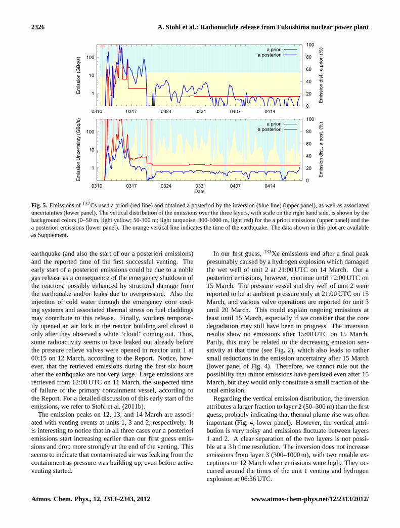
Fig. 9. Scatter plot of observed and simulated137Cs concentrations, based on a priori (red squares) and a posteriori (blue crosses) emissions.The gray line in the middle is the 1:1 line and upper and lower lines represent factor of 5 over- and underestimates.
of 1×10⁻⁴ Bq m−3 to every simulated concentration. Thiswas done also to allow plotting of otherwise zero concen-tration values on the logarithmic plot. Consequently, onecannot expect any correlation between measured and simu-lated values in the lower left part of Fig.7, which is domi-nated by background variability outside the FD-NPP plume.Some of the observed values, for which the correspondingsimulated values are below 2×10⁻⁴ Bq m−3, are clearly ele-vated. As background values at some stations can reach sev-eral mBq m−3, many of these data points probably indicatean enhanced background rather than that the model did notcapture the FD-NPP plume.
Data points in the upper right part of the figure all reflectthe emissions from FD-NPP and for these data points, themodeled and observed values show a tight correlation. Mostof the simulated values fall within a factor of five of the ob-served values. While the model results using our first guessemissions are already well correlated with the measurements,the inversion clearly improves the correspondence, with mostof the data points falling closer to the 1:1 line.
Comparisons between simulated and observed time seriesof 133Xe are shown at the example of Richland, Oahu andStockholm (Fig.8). The locations of these sites are shown inFig. 13 (see also Table4). At Richland (Fig.8, top panel),the plume first arrived on 16 March. The arrival time iswell simulated but the modeled values drop back to nearlybackground on 17 March before rising again, whereas themeasured concentrations increase continuously. At the sta-tion Sidney (not shown), which is relatively close to Rich-land, the measurements in fact show a similar behavior as ourmodel results for Richland. At Richland, the model overesti-mates the measured peak concentrations on 19–20 March by
a factor of about three, whereas at Sidney it underpredicted.Since the two stations sampled the same part of the radioac-tive cloud, the inversion could not bring the model resultsin agreement with the measurements at both stations. Over-all, however, the model captures the133Xe variability at bothsites quite well. The time series also shows the formation ofa hemispheric cloud of133Xe. After arrival of the FD-NPPplume at Richland, there is considerable concentration vari-ability which decreases rapidly as133Xe becomes uniformlydistributed throughout the Northern Hemisphere. The steadyconcentration decrease in April is mainly due to radioactivedecay but also some further mixing into the tropical and polaratmospheres.
At Oahu (Fig.8, middle panel), which is closer to Japanthan Richland, the first detection of the FD-NPP plume wasmade later than at Richland, on 19 March. This happened be-cause this part of the radioactive cloud was first transportedto the eastern North Pacific in the midlatitudes, before curv-ing to the south and then to the west. Again, the timing ofthe plume arrival is well captured, although the model ini-tially underestimates the measured concentrations but thenoverpredicts the first measured peak. The model success-fully captures a 1-day concentration minimum on 22 Marchand also some subsequent concentration variability.
At Stockholm (Fig.8, bottom panel), the plume arrived on22 March and this was also very well captured by the model.Simulated concentrations are within a factor of two to theobservations and the inversion brings the simulated valuescloser to the observations most of the time. Before the ar-rival of the FD-NPP plume, the model simulations underes-timate the observations, a consequence of a too low back-ground added to the model results.
Atmos. Chem. Phys., 12, 2313–2343, 2012 www.atmos-chem-phys.net/12/2313/2012/

A. Stohl et al.: Radionuclide release from Fukushima nuclear power plant 2331
4.3.2 Caesium-137
Figure 9 compares measured and simulated137Cs concen-trations. Again, a random, normally distributed backgroundconcentration was added to every simulated concentrationvalue. Typical background values in Europe are of the or-der of 0.5 µBq m−3 (Valles et al., 2009), which was used forthe standard deviation of the random values. The agreementbetween the model and the observations is worse than for133Xe, a consequence of the added complexity of modelingwet and dry removal of the particles carrying137Cs. How-ever, there is still a clear correlation between modeled andobserved concentrations and the inversion further improvesthe agreement, especially for the highest concentration val-ues.
Figure 10 shows time series of measured and modeled137Cs concentrations at Tokai-mura, Oahu and Stockholm(station locations are shown in Fig.14, see also Table5).At Tokai-mura (Fig.10, top panel), the plume arrivals on14, 21 and 30 March as well as several peaks in April arewell captured by the model, although the differences betweenmeasured and modeled concentrations are often substantial.The simulated concentrations drop to background levels inbetween plume passages, whereas measured concentrationsremain strongly elevated, especially in March after the mostheavy contamination events. Possible causes are the resus-pension of137Cs from contaminated surfaces (see alsoYa-mauchi, 2012), which is not treated in our model, and detec-tor contamination similar to Takasaki. This behavior is alsoseen at the other Japanese stations.
At Oahu (Fig.10, middle panel), the main plume eventsare again captured, but the agreement between model andmeasurements is much worse than for133Xe. As for 133Xe,the model overpredicts the main concentration peaks for thissite.
At Stockholm (Fig.10, bottom panel), the model generallyoverpredicts in March and underpredicts in April. The lowmeasured concentrations between 22 and 27 March are sur-prising, given that the133Xe concentrations during that timeperiod are almost as high as at the end of March. There musthave been very strong wet scavenging of137Cs to explainthe low 137Cs/133Xe ratios. Indeed, the model simulationsshow that this part of the plume was lifted to the free tropo-sphere just downwind of Japan and then descended back tothe surface over the North Atlantic. The model must have un-derestimated the wet scavenging in this case. However, thisis not typical as otherwise the inversion would have reducedthe emissions to improve the agreement between the modeland the measurements.
Figure 11 shows a scatter plot of simulated versus ob-served137Cs deposition values. As for the concentrationdata, the data set is dominated by zero values and in thiscase there are also many zero observations. To show thesedata on the logarithmic plot, we added a normally distributedrandom value with a standard deviation of 1 Bq m−2 (day)−1
0.001
0.01
0.1
1
10
100
1000
0312 0319 0326 0402 0409 0416
137 C
s (B
q/m
3 )
Tokai-muraA priori
A posterioriObserved
1e-006
1e-005
0.0001
0.001
0.01
0312 0319 0326 0402 0409 0416
137 C
s (B
q/m
3 )
OahuA priori
A posterioriObserved
1e-006
1e-005
0.0001
0.001
0312 0319 0326 0402 0409 0416
137 C
s (B
q/m
3 )
StockholmA priori
A posterioriObserved
Fig. 10. Time series of observed (black line) and simulated137Csconcentrations, based on a priori (red line) and a posteriori (blueline) emissions, for the stations Tokai-mura (top panel), Oahu (mid-dle panel) and Stockholm (bottom panel).
to every zero observation and a random value with a standarddeviation of 2 Bq m−2 (day)−1 to every simulated deposition.Therefore, no correlation is expected for the data in the lowerleft part of the figure. There is not a particularly tight corre-lation between the observations and the model simulationsnear the high end of the data range. However, the modelhas little overall bias and the inversion clearly reduces thescatter. There are many cases for which the model suggestsbackground values but observations are enhanced. Again,we suspect this to be due to resuspension of previously de-posited137Cs or to contamination problems. However, some
www.atmos-chem-phys.net/12/2313/2012/ Atmos. Chem. Phys., 12, 2313–2343, 2012
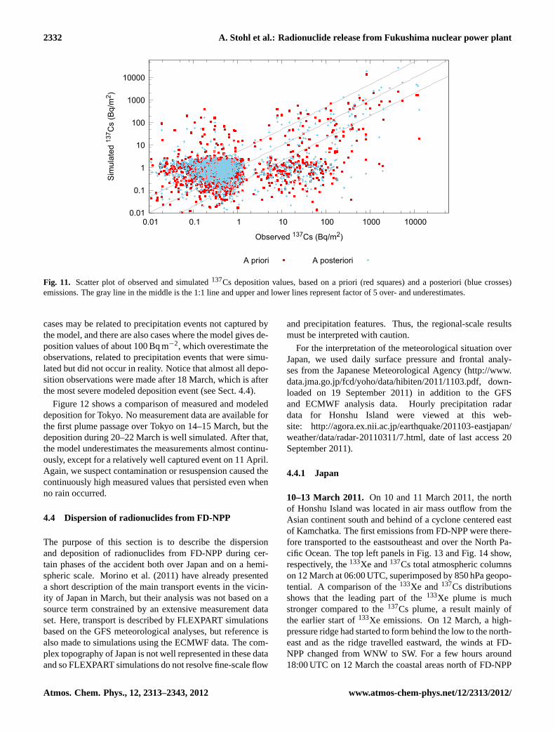
2332 A. Stohl et al.: Radionuclide release from Fukushima nuclear power plant
0.01
0.1
1
10
100
1000
10000
0.01 0.1 1 10 100 1000 10000
Sim
ulat
ed 13
7 Cs
(Bq/
m2 )
Observed 137Cs (Bq/m2)
A priori A posteriori
Fig. 11. Scatter plot of observed and simulated137Cs deposition values, based on a priori (red squares) and a posteriori (blue crosses)emissions. The gray line in the middle is the 1:1 line and upper and lower lines represent factor of 5 over- and underestimates.
cases may be related to precipitation events not captured bythe model, and there are also cases where the model gives de-position values of about 100 Bq m−2, which overestimate theobservations, related to precipitation events that were simu-lated but did not occur in reality. Notice that almost all depo-sition observations were made after 18 March, which is afterthe most severe modeled deposition event (see Sect.4.4).
Figure12 shows a comparison of measured and modeleddeposition for Tokyo. No measurement data are available forthe first plume passage over Tokyo on 14–15 March, but thedeposition during 20–22 March is well simulated. After that,the model underestimates the measurements almost continu-ously, except for a relatively well captured event on 11 April.Again, we suspect contamination or resuspension caused thecontinuously high measured values that persisted even whenno rain occurred.
4.4 Dispersion of radionuclides from FD-NPP
The purpose of this section is to describe the dispersionand deposition of radionuclides from FD-NPP during cer-tain phases of the accident both over Japan and on a hemi-spheric scale.Morino et al.(2011) have already presenteda short description of the main transport events in the vicin-ity of Japan in March, but their analysis was not based on asource term constrained by an extensive measurement dataset. Here, transport is described by FLEXPART simulationsbased on the GFS meteorological analyses, but reference isalso made to simulations using the ECMWF data. The com-plex topography of Japan is not well represented in these dataand so FLEXPART simulations do not resolve fine-scale flow
and precipitation features. Thus, the regional-scale resultsmust be interpreted with caution.
For the interpretation of the meteorological situation overJapan, we used daily surface pressure and frontal analy-ses from the Japanese Meteorological Agency (http://www.data.jma.go.jp/fcd/yoho/data/hibiten/2011/1103.pdf, down-loaded on 19 September 2011) in addition to the GFSand ECMWF analysis data. Hourly precipitation radardata for Honshu Island were viewed at this web-site: http://agora.ex.nii.ac.jp/earthquake/201103-eastjapan/weather/data/radar-20110311/7.html, date of last access 20September 2011).
4.4.1 Japan
10–13 March 2011. On 10 and 11 March 2011, the northof Honshu Island was located in air mass outflow from theAsian continent south and behind of a cyclone centered eastof Kamchatka. The first emissions from FD-NPP were there-fore transported to the eastsoutheast and over the North Pa-cific Ocean. The top left panels in Fig.13 and Fig.14 show,respectively, the133Xe and137Cs total atmospheric columnson 12 March at 06:00 UTC, superimposed by 850 hPa geopo-tential. A comparison of the133Xe and137Cs distributionsshows that the leading part of the133Xe plume is muchstronger compared to the137Cs plume, a result mainly ofthe earlier start of133Xe emissions. On 12 March, a high-pressure ridge had started to form behind the low to the north-east and as the ridge travelled eastward, the winds at FD-NPP changed from WNW to SW. For a few hours around18:00 UTC on 12 March the coastal areas north of FD-NPP
Atmos. Chem. Phys., 12, 2313–2343, 2012 www.atmos-chem-phys.net/12/2313/2012/
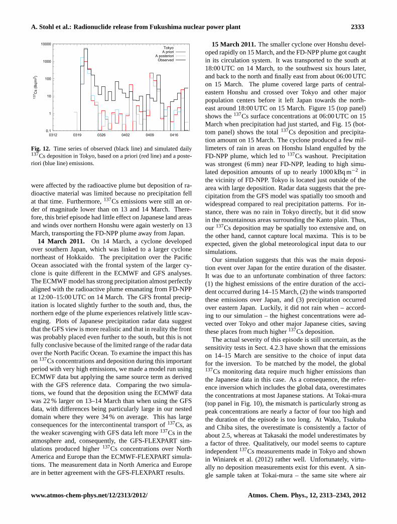
A. Stohl et al.: Radionuclide release from Fukushima nuclear power plant 2333
0.1
1
10
100
1000
10000
0312 0319 0326 0402 0409 0416
137 C
s (B
q/m
2 )
TokyoA priori
A posterioriObserved
Fig. 12. Time series of observed (black line) and simulated daily137Cs deposition in Tokyo, based on a priori (red line) and a poste-riori (blue line) emissions.
were affected by the radioactive plume but deposition of ra-dioactive material was limited because no precipitation fellat that time. Furthermore,137Cs emissions were still an or-der of magnitude lower than on 13 and 14 March. There-fore, this brief episode had little effect on Japanese land areasand winds over northern Honshu were again westerly on 13March, transporting the FD-NPP plume away from Japan.
14 March 2011. On 14 March, a cyclone developedover southern Japan, which was linked to a larger cyclonenortheast of Hokkaido. The precipitation over the PacificOcean associated with the frontal system of the larger cy-clone is quite different in the ECMWF and GFS analyses.The ECMWF model has strong precipitation almost perfectlyaligned with the radioactive plume emanating from FD-NPPat 12:00–15:00 UTC on 14 March. The GFS frontal precip-itation is located slightly further to the south and, thus, thenorthern edge of the plume experiences relatively little scav-enging. Plots of Japanese precipitation radar data suggestthat the GFS view is more realistic and that in reality the frontwas probably placed even further to the south, but this is notfully conclusive because of the limited range of the radar dataover the North Pacific Ocean. To examine the impact this hason137Cs concentrations and deposition during this importantperiod with very high emissions, we made a model run usingECMWF data but applying the same source term as derivedwith the GFS reference data. Comparing the two simula-tions, we found that the deposition using the ECMWF datawas 22 % larger on 13–14 March than when using the GFSdata, with differences being particularly large in our nesteddomain where they were 34 % on average. This has largeconsequences for the intercontinental transport of137Cs, asthe weaker scavenging with GFS data left more137Cs in theatmosphere and, consequently, the GFS-FLEXPART sim-ulations produced higher137Cs concentrations over NorthAmerica and Europe than the ECMWF-FLEXPART simula-tions. The measurement data in North America and Europeare in better agreement with the GFS-FLEXPART results.
15 March 2011.The smaller cyclone over Honshu devel-oped rapidly on 15 March, and the FD-NPP plume got caughtin its circulation system. It was transported to the south at18:00 UTC on 14 March, to the southwest six hours later,and back to the north and finally east from about 06:00 UTCon 15 March. The plume covered large parts of central-eastern Honshu and crossed over Tokyo and other majorpopulation centers before it left Japan towards the north-east around 18:00 UTC on 15 March. Figure15 (top panel)shows the137Cs surface concentrations at 06:00 UTC on 15March when precipitation had just started, and Fig.15 (bot-tom panel) shows the total137Cs deposition and precipita-tion amount on 15 March. The cyclone produced a few mil-limeters of rain in areas on Honshu Island engulfed by theFD-NPP plume, which led to137Cs washout. Precipitationwas strongest (6 mm) near FD-NPP, leading to high simu-lated deposition amounts of up to nearly 1000 kBq m−2 inthe vicinity of FD-NPP. Tokyo is located just outside of thearea with large deposition. Radar data suggests that the pre-cipitation from the GFS model was spatially too smooth andwidespread compared to real precipitation patterns. For in-stance, there was no rain in Tokyo directly, but it did snowin the mountainous areas surrounding the Kanto plain. Thus,our 137Cs deposition may be spatially too extensive and, onthe other hand, cannot capture local maxima. This is to beexpected, given the global meteorological input data to oursimulations.
Our simulation suggests that this was the main deposi-tion event over Japan for the entire duration of the disaster.It was due to an unfortunate combination of three factors:(1) the highest emissions of the entire duration of the acci-dent occurred during 14–15 March, (2) the winds transportedthese emissions over Japan, and (3) precipitation occurredover eastern Japan. Luckily, it did not rain when – accord-ing to our simulation – the highest concentrations were ad-vected over Tokyo and other major Japanese cities, savingthese places from much higher137Cs deposition.
The actual severity of this episode is still uncertain, as thesensitivity tests in Sect.4.2.3have shown that the emissionson 14–15 March are sensitive to the choice of input datafor the inversion. To be matched by the model, the global137Cs monitoring data require much higher emissions thanthe Japanese data in this case. As a consequence, the refer-ence inversion which includes the global data, overestimatesthe concentrations at most Japanese stations. At Tokai-mura(top panel in Fig.10), the mismatch is particularly strong aspeak concentrations are nearly a factor of four too high andthe duration of the episode is too long. At Wako, Tsukubaand Chiba sites, the overestimate is consistently a factor ofabout 2.5, whereas at Takasaki the model underestimates bya factor of three. Qualitatively, our model seems to captureindependent137Cs measurements made in Tokyo and shownin Winiarek et al.(2012) rather well. Unfortunately, virtu-ally no deposition measurements exist for this event. A sin-gle sample taken at Tokai-mura – the same site where air
www.atmos-chem-phys.net/12/2313/2012/ Atmos. Chem. Phys., 12, 2313–2343, 2012
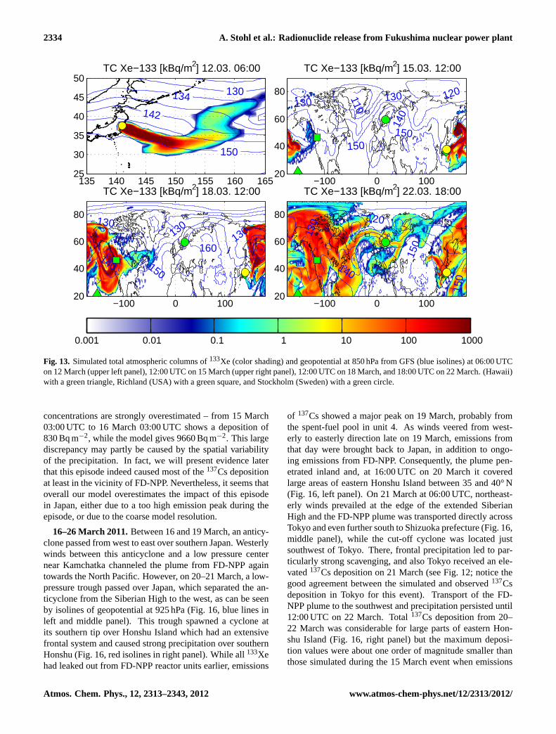
2334 A. Stohl et al.: Radionuclide release from Fukushima nuclear power plant
TC Xe−133 [kBq/m2] 12.03. 06:00
150
142
134 130
135 140 145 150 155 160 16525
30
35
40
45
50TC Xe−133 [kBq/m2] 15.03. 12:00
120
150150
130
110
140
130
−100 0 10020
40
60
80
TC Xe−133 [kBq/m2] 18.03. 12:00
150
160130130
140
130
−100 0 10020
40
60
80
TC Xe−133 [kBq/m2] 22.03. 18:00
140
120
150
150
130
−100 0 10020
40
60
80
0.001 0.01 0.1 1 10 100 1000
Fig. 13. Simulated total atmospheric columns of133Xe (color shading) and geopotential at 850 hPa from GFS (blue isolines) at 06:00 UTCon 12 March (upper left panel), 12:00 UTC on 15 March (upper right panel), 12:00 UTC on 18 March, and 18:00 UTC on 22 March. (Hawaii)with a green triangle, Richland (USA) with a green square, and Stockholm (Sweden) with a green circle.
concentrations are strongly overestimated – from 15 March03:00 UTC to 16 March 03:00 UTC shows a deposition of830 Bq m−2, while the model gives 9660 Bq m−2. This largediscrepancy may partly be caused by the spatial variabilityof the precipitation. In fact, we will present evidence laterthat this episode indeed caused most of the137Cs depositionat least in the vicinity of FD-NPP. Nevertheless, it seems thatoverall our model overestimates the impact of this episodein Japan, either due to a too high emission peak during theepisode, or due to the coarse model resolution.
16–26 March 2011.Between 16 and 19 March, an anticy-clone passed from west to east over southern Japan. Westerlywinds between this anticyclone and a low pressure centernear Kamchatka channeled the plume from FD-NPP againtowards the North Pacific. However, on 20–21 March, a low-pressure trough passed over Japan, which separated the an-ticyclone from the Siberian High to the west, as can be seenby isolines of geopotential at 925 hPa (Fig.16, blue lines inleft and middle panel). This trough spawned a cyclone atits southern tip over Honshu Island which had an extensivefrontal system and caused strong precipitation over southernHonshu (Fig.16, red isolines in right panel). While all133Xehad leaked out from FD-NPP reactor units earlier, emissions
of 137Cs showed a major peak on 19 March, probably fromthe spent-fuel pool in unit 4. As winds veered from west-erly to easterly direction late on 19 March, emissions fromthat day were brought back to Japan, in addition to ongo-ing emissions from FD-NPP. Consequently, the plume pen-etrated inland and, at 16:00 UTC on 20 March it coveredlarge areas of eastern Honshu Island between 35 and 40° N(Fig. 16, left panel). On 21 March at 06:00 UTC, northeast-erly winds prevailed at the edge of the extended SiberianHigh and the FD-NPP plume was transported directly acrossTokyo and even further south to Shizuoka prefecture (Fig.16,middle panel), while the cut-off cyclone was located justsouthwest of Tokyo. There, frontal precipitation led to par-ticularly strong scavenging, and also Tokyo received an ele-vated137Cs deposition on 21 March (see Fig.12; notice thegood agreement between the simulated and observed137Csdeposition in Tokyo for this event). Transport of the FD-NPP plume to the southwest and precipitation persisted until12:00 UTC on 22 March. Total137Cs deposition from 20–22 March was considerable for large parts of eastern Hon-shu Island (Fig.16, right panel) but the maximum deposi-tion values were about one order of magnitude smaller thanthose simulated during the 15 March event when emissions
Atmos. Chem. Phys., 12, 2313–2343, 2012 www.atmos-chem-phys.net/12/2313/2012/
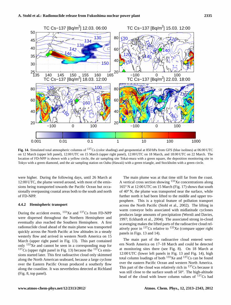
A. Stohl et al.: Radionuclide release from Fukushima nuclear power plant 2335
TC Cs−137 [Bq/m2] 12.03. 06:00
150
146142
138134
130
135 140 145 150 155 160 16525
30
35
40
45
50TC Cs−137 [Bq/m2] 15.03. 12:00
150
120
120 120
140140
140
110
−100 0 10020
40
60
80
TC Cs−137 [Bq/m2] 18.03. 12:00
150
140 160 130
100120
−100 0 10020
40
60
80
TC Cs−137 [Bq/m2] 22.03. 18:00
150
130
140
130
130
150
−100 0 10020
40
60
80
0.001 0.01 0.1 1 10 100 1000
Fig. 14. Simulated total atmospheric columns of137Cs (color shading) and geopotential at 850 hPa from GFS (blue isolines) at 06:00 UTCon 12 March (upper left panel), 12:00 UTC on 15 March (upper right panel), 12:00 UTC on 18 March, and 18:00 UTC on 22 March. Thelocation of FD-NPP is shown with a yellow circle, the air sampling site Tokai-mura with a green square, the deposition monitoring site inTokyo with a green diamond, and the air sampling station on Oahu (Hawaii) with a green triangle, and Stockholm with a green circle.
were higher. During the following days, until 26 March at12:00 UTC, the plume veered around, with most of the emis-sions being transported towards the Pacific Ocean but occa-sionally overpassing coastal areas both to the south and northof FD-NPP.
4.4.2 Hemispheric transport
During the accident events,133Xe and137Cs from FD-NPPwere dispersed throughout the Northern Hemisphere andeventually also reached the Southern Hemisphere. A firstradionuclide cloud ahead of the main plume was transportedquickly across the North Pacific at low altitudes in a steadywesterly flow and arrived in western North America on 15March (upper right panel in Fig.13). This part containedonly 133Xe and cannot be seen in a corresponding map for137Cs (upper right panel in Fig.13) because the137Cs emis-sions started later. This first radioactive cloud only skimmedalong the North American seaboard, because a large cycloneover the Eastern Pacific Ocean produced a southerly flowalong the coastline. It was nevertheless detected at Richland(Fig. 8, top panel).
The main plume was at that time still far from the coast.A vertical cross section showing133Xe concentrations along165° N at 12:00 UTC on 15 March (Fig.17) shows that southof 40° N, the plume was transported near the surface, whilefurther north it had been lifted to the middle and upper tro-posphere. This is a typical feature of pollution transportacross the North Pacific (Stohl et al., 2002). The lifting inwarm conveyor belts associated with midlatitude cyclonesproduces large amounts of precipitation (Wernli and Davies,1997; Eckhardt et al., 2004). The associated strong in-cloudscavenging makes the lifted parts of the radioactive cloud rel-atively poor in137Cs relative to133Xe (compare upper rightpanels in Figs.13and14).
The main part of the radioactive cloud entered west-ern North America on 17–18 March and could be detectedat monitoring sites there (see Fig.8). On 18 March at12:00 UTC (lower left panels in Fig.13 and Fig.14), hightotal column loadings of both133Xe and137Cs can be foundover the eastern Pacific Ocean and western North America.This part of the cloud was relatively rich in137Cs because itwas still close to the surface south of 50°. The high-altitudehead of the cloud with lower column values of137Cs had
www.atmos-chem-phys.net/12/2313/2012/ Atmos. Chem. Phys., 12, 2313–2343, 2012

2336 A. Stohl et al.: Radionuclide release from Fukushima nuclear power plant
already arrived over the North Atlantic. At the same time,the radioactive cloud penetrated the subtropics and arrived atHawaii on 19 March (see also Fig.10).
Emissions from FD-NPP first arrived over Europe on 20March, however only at high altitudes. Surface measure-ments at Stockholm revealed enhanced133Xe concentrationsfirst on 22 March (bottom panel in Fig.8). A map of the sim-ulated surface concentrations of133Xe (Fig.18) for 22 Marchshows that all of western North America was engulfed bythe FD-NPP plume, as well as parts of eastern North Amer-ica and eastern Asia. At that time, Europe was still free ofenhanced133Xe at the surface, except for an isolated133Xecloud over Scandinavia. Transport movies show that the con-taminated air had been transported in the middle and uppertroposphere and descended south of Iceland, just 12 h beforearriving over Scandinavia. A comparison of total columnsof 133Xe and 137Cs shows that this air is predicted to berich in 133Xe but relatively poor in137Cs, due to wet scav-enging during uplift (lower right panels in Figs.13 and14).The measurements (see Fig.10) show that the137Cs concen-trations were even lower than predicted, suggesting that themodel underestimated the wet scavenging in this case.
The total column plots (lower right panels in Figs.13and14) show that on 22 March, contaminated air from FD-NPP had circled the entire Northern Hemisphere and hadreached both the tropics as well as the polar regions. Eventhough enhanced surface concentrations were still limitedto smaller parts of the Northern Hemisphere (Fig.18), thischanged quickly. In April all measurement stations recordedan enhanced (but due to radioactive decay, decreasing) back-ground of133Xe caused by the FD-NPP emissions, indicatingthe transition to complete dispersion in the Northern Hemi-sphere (seeStohl et al., 2012). Even the Australian sta-tion Darwin started recording enhanced133Xe concentrationsin April, indicating penetration of radioactive contaminationinto the Southern Hemisphere.
Total deposition. Figure 19 shows maps of total depo-sition of 137Cs in Japan and globally. The highest FD-NPPdeposition values of about 1000 kBq m−2 occur in a plumestretching from FD-NPP to the northwest. The orientation ofthis simulated plume is exactly as found by aerial surveys of137Cs surface deposition inside a radius of about 100–130 kmaround FD-NPP using several aircraft between 6 April and26 May 2011 (MEXT, 2011). The airborne measurementsshow that along the main plume axis,137Cs deposition val-ues greater than 1000 kBq m−2 extend about 50 km from FD-NPP. This is consistent with our results both in terms of depo-sition magnitude and extension, but a more detailed compar-ison is difficult because the measured deposition is spatiallyhighly variable on scales of a few kilometers, and this cannotbe resolved by our model. Since the modeled137Cs total de-position is mainly due to the deposition event on 15 March,the agreement of deposition patterns with the airborne obser-vations suggests that 15 March was correctly identified withour model as the strongest deposition episode. Given that al-
Surface conc. Cs−137 [Bq/m3] 15.03. 06:00
70
70
70
69
138 139 140 141 142 143 144 14533
34
35
36
37
38
39
40
Deposition Cs−137 [kBq/m2] 15.03. 00:00 to 16.03. 00:00
2
3
35
4
2
6
1
1
1
1
138 139 140 141 142 143 144 14532
33
34
35
36
37
38
39
40
0.001 0.01 0.1 1 10 100 1000
Fig. 15. Simulated surface concentrations of137Cs (color shading)and 925 hPa geopotential from GFS (blue isolines) at 06:00 UTCon 15 March (upper panel), as well as total137Cs deposition (colorshading) and accumulated precipitation from 00:00–24:00 UTC on15 March (lower panel). The location of FD-NPP is shown with ayellow circle, the air sampling site Tokai-mura with a green square,and the deposition monitoring site in Tokyo with a green diamond.
most no deposition measurements were made on 15 March,this is an important confirmation.
Our maps of total137Cs deposition are quite differentfrom those presented byYasunari et al.(2011), which showsmaller deposition amounts. This can be explained by thefact thatYasunari et al.(2011) only had sufficient depositiondata available for their study starting from 20 March, and thatdoes not include the most severe deposition event accordingto our study, on 15 March. In fact, their Fig. 2 is quite similarto our deposition map for 20–22 March (left panel in Fig.16).
To put our findings into perspective, a comparison withthe Chernobyl disaster is quite interesting. Followingthe Chernobyl accident,137Cs deposition values exceeding1000 kBq m−2 were observed in two areas, namely in theexclusion zone around Chernobyl NPP/Prypjat and north ofthe city of Gomel in Belarus (see deposition maps inUN-SCEAR, 2000b). For the FD-NPP accident, the land areasreceiving such high deposition values are smaller, but theyare still extensive. Another comparison of interest is with the137Cs deposition in the extratropical Northern Hemispherestill present due to past nuclear testing, about 1–2 kBq m−2
Atmos. Chem. Phys., 12, 2313–2343, 2012 www.atmos-chem-phys.net/12/2313/2012/

A. Stohl et al.: Radionuclide release from Fukushima nuclear power plant 2337
Surface conc. Cs−137 [Bq/m3] 20.03. 16:00
7978
77
7675
7473
72
135 140 14532
33
34
35
36
37
38
39
40
41
42
Surface conc. Cs−137 [Bq/m3] 21.03. 06:00
7172
73
74
72
7375
135 140 14532
33
34
35
36
37
38
39
40
41
42
Deposition Cs−137 [kBq/m2] 20.03. 00:00 to 22.03. 12:00
12
8
2
4
814
12
4
1
1010
135 140 14532
33
34
35
36
37
38
39
40
41
42
0.001 0.01 0.1 1 10 100 1000
Fig. 16. Simulated surface concentrations of137Cs at 16:00 UTC on 20 March (color shading) and 925 hPa geopotential from GFS (blueisolines) at 15:00 UTC on 20 March (left panel) and at 06:00 UTC on 21 March (middle panel), as well as total137Cs deposition (colorshading) and accumulated precipiation (in mm, red lines) from 00:00 UTC on 20 March to 12:00 UTC on 22 March (right panel). Thelocation of FD-NPP is shown with a yellow circle, the air sampling site Tokai-mura with a green square, and the deposition monitoring sitein Tokyo with a green diamond.
Hei
ght a
gl [k
m]
Cross section at 165 E Xe−133 [Bq/m3] 15.03. 12:00
30 35 40 45 50 55 600
1
2
3
4
5
6
7
8
9
10
0.001 0.01 0.1 1 10 100 1000
Fig. 17. Vertical cross section along 165°E through the model out-put for 133Xe at 12:00 UTC on 15 March.
(UNSCEAR, 2000a). That value is exceeded by depositionfrom FD-NPP over large parts of Honshu Island and the west-ern Pacific Ocean. However, deposition of FD-NPP137Csemissions over other parts of Asia, North America and Eu-rope is minor compared to this pre-existing background.
To determine the deposition amounts in Japan and otherregions, we combined our gridded accumulated deposition
fields on 20 April at 00:00 UTC (decay-corrected for thattime) with a land-sea mask. This analysis accounts for morethan 90 % of the137Cs emissions until 20 April, with the reststill residing in the atmosphere and small amounts destroyedby radioactive decay. We find that Japanese land areas re-ceived 6.4 PBq, or 18 % of the total137Cs deposition until 20April. The relative fraction deposited in Japan is quite similarto the 22 % reported byMorino et al.(2011), although theirabsolute values are smaller because of lower emissions used.Only 0.7 PBq, or 1.9 % of the total137Cs deposition occurredover land areas other than Japan, while the remaining 80 %were deposited in the oceans.
5 Conclusions
In this study, we estimated the total releases of the radioac-tive isotopes133Xe and137Cs as well as their temporal emis-sion patterns from the damaged Fukushima Dai-ichi nuclearpower plant (FD-NPP) in March and April 2011. The es-timate is based on an inverse modeling method, using thetransport model FLEXPART and a large number of avail-able concentration and deposition measurements in Japan,North America, Europe, and a few other locations. De-spite the significant uncertainties in simulations as well asmeasurements, the inversion method was able to produce
www.atmos-chem-phys.net/12/2313/2012/ Atmos. Chem. Phys., 12, 2313–2343, 2012

2338 A. Stohl et al.: Radionuclide release from Fukushima nuclear power plant
Surface conc. Xe−133 [Bq/m3] 22.03. 18:00
70
8090
60
5040
50
55 45
80
70
75
7075
7090
70
60
−150 −100 −50 0 50 100 15020
30
40
50
60
70
80
90
0.001 0.01 0.1 1 10 100 1000
Fig. 18. Surface concentrations of 133Xe (color shading) and geopotential at 925 hPa (blue isolines) at 18 UTC
on 22 March. In the lower panel, the stations Oahu (Hawaii) and Stockholm (Sweden) are marked with a green
triangle and a green circle, respectively.
57
Fig. 18.Surface concentrations of133Xe (color shading) and geopotential at 925 hPa (blue isolines) at 18:00 UTC on 22 March. In the lowerpanel, the stations Oahu (Hawaii) and Stockholm (Sweden) are marked with a green triangle and a green circle, respectively.
model results that are largely consistent with the measure-ment data.
Regarding the noble gas133Xe, it is almost certain thatthe accumulated inventory of the reactor units 1-3 was com-pletely set free into the atmosphere between 11 and 15March. The study indicates a total release of 15.3 (uncer-tainty range 12.2-18.3) EBq, more than the estimated inven-tory of 12.4 EBq133Xe. We explain this with the additionaldecay of133I into 133Xe, which would effectively increasethe estimated inventory to 14.4 EBq133Xe. This release ismore than a factor of two higher than the Chernobyl133Xesource term and most likely the largest radioactive noble gasrelease in history. There is also strong evidence that the startof the release occurred early, before the first active ventingwas made. This early onset of emissions is interesting andmight indicate some structural damage to the reactor unitsby the earthquake.
Regarding137Cs, the inversion results indicate a totalemission of 36.6 (20.1–53.1) PBq, or about 43 % of the es-timated Chernobyl emission. This means that nearly 2 % ofthe available inventory of the reactor cores in units 1–3 andthe spent-fuel pool in unit 4 was discharged into the atmo-sphere. The inversion strongly increased the emissions earlyon 12 March, around the time when the first explosion oc-curred in unit 1. These early emissions were estimated lowerby the Japanese authorities, but are in accordance with thefirst estimates published byCentral Institute for Meteorologyand Geodynamics(2011). The highest release rates occurred
on 14 March, when hydrogen explosions occurred in reac-tor units 3 and 4 and, presumably, unit 2. We also find un-expectedly high137Cs emissions from 16–19 March, whichsuddenly dropped by orders of magnitude when spraying ofwater on the spent-fuel pool of unit 4 started. Thus, we be-lieve that these high emissions are related to the degradedfuel in the spent-fuel pool of unit 4, and this result wouldalso confirm that the spraying was an effective countermea-sure at least in this case. Between 19 March and 10 April,episodic but generally decreasing emissions were found.
The winds transported the FD-NPP emissions towards thePacific Ocean most of the time, while Japan was affectedonly occasionally. While this seemed like a relatively for-tunate situation for Japan during the accident event, a dif-ferent picture emerges from our detailed analysis. Exactlyduring and following the period of the highest137Cs emis-sion rates on 14 and 15 March, the FD-NPP plume was ad-vected towards Japan and affected large areas in the east ofHonshu Island. The advection towards Japan was triggeredby a developing cyclone, which produced precipitation on 15March, leading to the deposition of large fractions of the air-borne137Cs over Japanese land. However, the situation couldhave been even much worse, as fortunately no rain occurredat the time when the FD-NPP plume was transported overTokyo. Our model seems to overestimate the impact of thisepisode in Japan, either due to an emission overestimate on14–15 March, or insufficient model resolution.
Atmos. Chem. Phys., 12, 2313–2343, 2012 www.atmos-chem-phys.net/12/2313/2012/

A. Stohl et al.: Radionuclide release from Fukushima nuclear power plant 2339
Total Deposition Cs−137 [kBq/m2]
70
60
50
40
40
2030
40
138 139 140 141 142 143 144 14532
34
36
38
40
42
−150 −100 −50 0 50 100 15020
30
40
50
60
70
80
90
0.001 0.01 0.1 1 10 100 1000
Fig. 19. Maps of total deposition of137Cs until 20 April00:00 UTC, for Japan (upper panel) and the global domain (lowerpanel). Superimposed on the upper panel is the total precipitationfrom GFS for the same time period. The location of FD-NPP isshown with a yellow circle, the air sampling site Tokai-mura witha green square, and the deposition monitoring site in Tokyo with agreen diamond. In the lower panel, the stations Oahu (Hawaii) andStockholm (Sweden) are marked with a green triangle and a greencircle, respectively.
During a second episode from 20–22 March, even largerareas of Honshu were covered by the FD-NPP radioac-tive cloud, from Shizuoka prefecture in the south to areasnorth of FD-NPP. Strong frontal precipitation nearly com-pletely cleansed the atmosphere of137Cs and again producedstrong deposition of this radionuclide over Honshu, includingTokyo. This episode again followed a period of high (thoughfortunately not as high as on 14–15 March)137Cs emissionfluxes on 19 March, which were transported to Japan on 20March. There were a few other periods when the FD-NPPplume was advected over land, but the areas affected weresmaller and the emissions lower, resulting in minor contami-nation compared to 15 and 20–21 March.
The emissions from FD-NPP were quickly dispersed inthe entire Northern Hemisphere. Already on 15 March, afirst isolated133Xe cloud reached western North America,followed by the arrival of high concentrations of both133Xeand 137Cs on 19 March. Europe was first reached on 22March by an air mass rich in133Xe but relatively poor in137Cs, which had been lifted in a frontal system over theNorth Pacific, was transported aloft and descended againover the North Atlantic shortly before reaching NorthernEurope. Precipitation associated with the frontal lifting had
removed most of the137Cs, but the noble gas133Xe remainedin the air mass. Higher137Cs concentrations reached Eu-rope at the end of March. By middle of April,133Xe wasfairly uniformly distributed in the middle latitudes of theentire Northern Hemisphere and was for the first time alsomeasured in the Southern Hemisphere (Darwin station, Aus-tralia).
A quantitative analysis of the model output shows that18 % of the total137Cs deposition until 20 April occurredover Japanese land. Only 0.7 PBq, or 1.9 % of the total de-position were received by land areas other than Japan, whilethe remaining 80 % were deposited in the oceans.
6 Needs for open data policy and further research
While we have collected measurement data from a variety ofsources, virtually none of these data sets is publicly available,and there are probably more useful data sets that were notaccessible to us. Institutions having produced relevant mea-surement data should make them freely available. A centraldata repository should be created where these data are beingstored, quality assured, reformatted to a common format andmade available to the general public. This will allow consid-erable improvements of the source terms in the future.
We have derived the source terms for two important ra-dionuclides. However, this needs to be done also for otherradionuclides, notably iodine-131.
We have used a global model for our study. Futurestudies should apply a nesting approach, where high res-olution can be achieved over Japan. This would facili-tate a more accurate simulation of radionuclide transportover Japan, which is important for assessing the impacts onhuman population. Importantly, this would also allow moreaccurate inverse modeling since better use of the Japanesemeasurement data could be made with reduced model errors.
There is a need for planned atmospheric tracer experi-ments to evaluate and further improve dispersion modelsused in emergency applications, as argued recently byGal-marini et al.(2011). There is also a need for careful check-ing and improvement of washout parameterizations in atmo-spheric dispersion models. The data set used in this papercould be useful in that respect.
Appendix A
Accident events at the different units
A1 Unit 1
On 14:00 UTC, 11 March (less than 8 h after the stationblackout) increased radiation was observed in the turbinehall, indicating that at least noble gases must have started toleak into the environment. At the same time, pressure built up
www.atmos-chem-phys.net/12/2313/2012/ Atmos. Chem. Phys., 12, 2313–2343, 2012

2340 A. Stohl et al.: Radionuclide release from Fukushima nuclear power plant
inside the containment and it is reported that between 00:15and 01:17 on 12 March relieve valves were opened, probablygiving rise to large releases. It is reported that at 05:30 on12 March the venting was finished. We assume that a largepart of the release has occured by then. At 06:36, the unit 1hydrogen explosion (which was the first one) happened, ob-viously from hydrogen that had entered various reactor build-ing compartments during the venting, or through leaks. Thecontainment pressure had dropped by 09:00 so that we as-sume the release was largely over at that time. Emissionswould likely continue at a lower rate through various leaksand at some point in time possibly also from the spent-fuelpond which after the explosion was directly exposed to theenvironment. On 14 March, a secondary pressure maximumin the containment was reported, possibly indicating another,minor, peak in the emissions.
A2 Unit 2
Unit 2 is of a newer design than unit 1 and was able to with-stand the station blackout somewhat longer. The first vent-ing for this unit is reported at 02:00 UTC on 13 March, withunclear success, and the first time of confirmed open safetyrelief valves is 09:00 UTC on 14 March. Radiation measure-ments in the wet well and dry well (reactor compartmentsbelow the pressure vessel, inside the containment) jumpedup about an hour later, probably indicating core melt, andalso MELCOR calculations give fuel melting for this time,as well as noble gas release. Thus we think that noble gaseshave been vented more or less completely at this time. At15:00 UTC, another venting of the dry well was performed,and a hydrogen explosion is suspected to have damaged thewet well at 21:14. Large releases appear likely. On 15March, 21:00 UTC, pressure vessel and dry well were at am-bient pressure, indicating the lack of any efficient barrier.The bulk of the discharge should have occurred by that time,but similar to unit 1, weak releases may continue. Between26 March and April 19 a secondary temperature increase inthe RPV was reported, possibly associated with somewhatincreased release.
A3 Unit 3
For unit 3, the first venting operation, through the wet well,is reported for 23:41 UTC on 11 March. This should alreadyhave released noble gases. About 24 h later, after observedincrease in the suppression chamber pressure, a second vent-ing of about 20 min was reported. On 13 March at 20:20the safety relief valves were reported open, and MELCORindicates pressure vessel failure around this time. Six hourslater, 02:00 UTC on 14 March, a very strong hydrogen ex-plosion occurred, severely damaging the upper part of thereactor building and scattering debris. The Report indicatesend of venting at 03:00 UTC. This should have ended thelarge release. However, until 20 March, various opening and
closing operations of the valves are reported which may havegiven rise to intermittent emission peaks on top of the slowerdischarge which is expected similar to unit 1. Finally, be-tween 1 April and 24 some secondary increase in pressurevessel temperatures was reported.
A4 Unit 4
Little information has been published on the spent fuel pondof unit 4 (which was the most critical one due to the highloading). Its water temperature was reported as 84 °C on 13March, 19:00 UTC. At such temperatures some release of ra-dionuclides is already likely. On 14 March, 21:00 UTC, amajor hydrogen explosion occurred in unit 4. This may ormay not have been caused by degraded fuel in the pond. It isreported that on 19 March, 23:21 UTC, spraying of water onthe pool was started. Having no further information, we sim-ply assumed a release fraction on the same order as for thereactor cores, less than 1 % of the caesium inventory, whichis thought to have mainly been released between hydrogenexplosion and the start of water spraying.
Supplement related to this article is available online at:http://www.atmos-chem-phys.net/12/2313/2012/acp-12-2313-2012-supplement.zip.
Acknowledgements.We would like to thank S. Furuta and M.Chino for providing137Cs concentration and deposition data fromTokai-mura; H. Haba for the Wako137Cs concentration data; K.Ungar and I. Hoffman for133Xe data from Sidney and137Cs datafrom Ottawa, Canada; H. Miley for133Xe data from Richland;S.-C. Hsu for data from Taiwanese stations; MEXT for providingthe137Cs deposition data from all Japanese prefectures; colleaguesfrom the Ro5 network for the Ro5 data; and all the researcherswho produced the CTBTO measurement data. Y. Yokouchi helpedlocating the data from Tsukuba and Chiba. M. Takigawa made theon-site dose rate measurements available in a convenient format.The second author is grateful for discussions with staff of theInstitute of Safety and Risk Sciences at BOKU. This work ispartly a spin-off of the project SOGG-EA (Sources of GreenhouseGases in East Asia) funded by the Norwegian Research Council.ECMWF and met.no granted access to ECMWF analysis data.
Edited by: H. Wernli
References
Andreev, I., Hittenberger, M., Hofer, P., Kromp-Kolb, H., Kromp,W., Seibert, P., and Wotawa, G.: Risks due to beyond design baseaccidents of nuclear power plants in Europe – the methodologyof Riskmap, J. Hazard. Mater., 61, 257–262, 1998.
Becker, A., Wotawa, G., Ringbom, A., and Saey, P. R. J.: Back-tracking of noble gas measurements taken in the aftermath of theannounced October 2006 event in North Korea by means of PTSmethods in nuclear source estimation and reconstruction, PureAppl. Geophys., 167, 581–599, 2010.
Atmos. Chem. Phys., 12, 2313–2343, 2012 www.atmos-chem-phys.net/12/2313/2012/

A. Stohl et al.: Radionuclide release from Fukushima nuclear power plant 2341
Bowyer, T. W., Biegalski, S. R., Cooper, M., Eslinger, P. W., Haas,D., Hayes, J. C., Miley, H. S., Strom, D. J., and Woods, V.: El-evated radioxenon detected remotely following the Fukushimanuclear accident, J. Environ. Radioact., 102, 681–687, 2011.
Brandt, J., Christensen, J. H., and Frohn, L. M.: Modelling transportand deposition of caesium and iodine from the Chernobyl acci-dent using the DREAM model, Atmos. Chem. Phys., 2, 397–417,doi:10.5194/acp-2-397-2002, 2002.
Central Institute for Meteorology and Geodynamics (ZAMG): Ac-cident in the Japanese NPP Fukushima: Spread of radioactiv-ity/first source estimates from CTBTO data show large sourceterms at the beginning of the accident/weather currently notfavourable/low level radioactivity meanwhile observed overU.S. East Coast and Hawaii,http://www.zamg.ac.at/docs/aktuell/Japan2011-03-221500E.pdf, last access: 28 September 2011.
Chino, M., Ishikawa, H., and Yamazawa, H.: SPEEDI andWSPEEDI: Japanese Emergency Response Systems to PredictRadiological Impacts in Local and Workplace Areas due to a Nu-clear Accident, Radiat. Prot. Dosimetry, 50, 145–152, 1993.
Chino, M., Nakayama, H., Nagai, H., Terada, H., Katata, G., andYamazawa, H.: Preliminary estimation of release amounts of131I and137Cs accidentally discharged from the Fukushima Dai-ichi nuclear power plant into the atmosphere, J. Nuc. Sci. Tech.,48, 1129–1134, 2011.
Davoine, X. and Bocquet, M.: Inverse modelling-based reconstruc-tion of the Chernobyl source term available for long-range trans-port, Atmos. Chem. Phys., 7, 1549–1564,doi:10.5194/acp-7-1549-2007, 2007.
Devell, L., Guntay, S., and Powers, D. A.: The Chernobyl Reac-tor Accident Source Term: Development of a Consensus View,CSNI Report, Organisation for Economic Co-Operation and De-velopment (OECD), OCDE/GD(96)12, 1995.
Eckhardt, S., Stohl, A., Wernli, H., James, P., Forster, C., andSpichtinger, N: A 15-year climatology of warm conveyor belts,J. Climate 17, 218–237, 2004.
Eckhardt, S., Prata, A. J., Seibert, P., Stebel, K., and Stohl, A.: Es-timation of the vertical profile of sulfur dioxide injection into theatmosphere by a volcanic eruption using satellite column mea-surements and inverse transport modeling, Atmos. Chem. Phys.,8, 3881–3897,doi:10.5194/acp-8-3881-2008, 2008.
Furuta, S., Sumiya, S., Watanabe, H., Nakano, M., Imaizumi,K., Takeyasu, M., Nakada, A., Fujita, H., Mizutani, T., Mori-sawa, M., Kokubun, Y., Kono, T., Nagaoka, M., Yokoyama, H.,Hokama, T., Isozaki, T., Nemoto, M., Hiyama, Y., Onuma, T.,Kato, C., and Kurachi, T.: Results of the Environmental Radia-tion Monitoring Following the Accident at the Fukushima Dai-ichi Nuclear Power Plant – Interim Report (Ambient RadiationDose Rate, Radioactivity Concentration in the Air and Radioac-tivity Concentration in the Fallout), Radiation Protection Depart-ment, Nuclear Fuel Cycle Engineering Laboratories, Tokai Re-search and Development Center, Japan Atomic Energy Agency,JAEA-Review 2011-035 (Draft), 2011.
Galmarini, S., Stohl, A., and Wotawa, G.: Fund experiments onatmospheric hazards, Nature, 473, p. 285, 2011.
Gauntt, R. O., Cole, R. K., Erickson, C. M., Gido, R. G., Gasser,R. D., Rodriguez, S. B., Young, M. F., Ashbaugh, S., Leonard,M., and Hill, A.: MELCOR Computer Code Manuals, Vol.3: Demonstration Problems, Version 1.8.5 May 2001, SandiaNational Laboratories, SAND2001-0929P, Albuquerque, USA,
2001.Gudiksen, P. H., Harvey, T. F., and Lange, R.: Chernobyl source
term, atmospheric dispersion, and dose estimation, Health Phys.,57, 697–706,1989.
Hartley, D. and Prinn, R.: Feasibility of determining surfaceemissions of trace gases using an inverse method in a three-dimensional chemical transport model, J. Geophys. Res., 98,5183–5197, 1993.
Hass, H., Memmesheimer, M., Geis, H., Jakobs, H. J., Laube, M.,and Ebel, A.: Simulation of the Chernobyl radioactive cloud overEurope using the EURAD model, Atmos. Environ., 24A, 673–692, 1990.
Hertel, O., Christensen, J. Runge, E. H., Asman,W. A. H., Berkow-icz, R., Hovmand, M. F., and Hov, O.: Development and testingof a new variable scale air pollution model – ACDEP, Atmos.Environ., 29, 1267–1290, 1995.
Hoffmann, W., Kebeasy, R., Firbas, P.: Introduction to the veri-fication regime of the Comprehensive Nuclear-Test-Ban Treaty,Phys. Earth Planet. Inter., 113, 5–9, 2000.
Hsu, S.-C., Huh, C.-A., Chan, C.-Y., Lin, S.-H., Lin, F.-J., and Liu,S. C.: Hemispheric dispersion of radioactive plume laced withfission nuclides from the Fukushima nuclear event, Geophys.Res. Lett., 39, L00G22,doi:10.1029/2011GL049986, 2012.
Institut de Radioprotection et de Surete Nucleaire (IRSN):IRSN publishes assessment of radioactivity released by theFukushima Daiichi Nuclear Power Plant (Fukushima I) through22 March 2011,http://www.irsn.fr/EN/news/Documents/IRSNfukushima-radioactivity-released-assessment-EN.pdf, last ac-cess: 28 September 2011, 2011.
Kirchner, G., Bossew, P., and De Cort, M.: Radioactivityfrom Fukushima Dai-ichi in air over Europe; part 2: whatcan it tell us about the accident? J. Environ. Radioact.,doi:10.1016/j.envrad.2011.12.016, in press, 2012.
Kristiansen, N. I., Stohl, A., Prata, A. J., Richter, A., Eckhardt, S.,Seibert, P., Hoffmann, A., Ritter, C., Bitar, L., Duck, T. J., andStebel, K.: Remote sensing and inverse transport modeling of theKasatochi eruption sulfur dioxide cloud, J. Geophys. Res., 115,D00L16,doi:10.1029/2009JD013286, 2010.
Mahowald, N. M., Prinn, R. G., and Rasch, P. J.: Deducing CCl3Femissions using an inverse method and chemical transport mod-els with assimilated winds, J. Geophys. Res., 102, 28153–28168,1997.
Masson, O., Baeza, A., Bieringer, J., Brudecki, K., Bucci, S., Cap-pai, M., Carvalho, F. P., Connan, O., Cosma, C., Dalheimer,A., D. Didier, G. Depuydt, L.E. De Geer, A. De Vismes, L.Gini, F. Groppi, K. Gudnason, R. Gurriaran, D. Hainz, Hall-dorsson, O., D. Hammond, O. Hanley, K. Holey, Zs. Homoki,A. Ioannidou, K. Isajenko, M. Jankovic, C. Katzlberger, M. Ket-tunen, R. Kierepko, R. Kontro, P.J.M. Kwakman, M. Lecomte,L. Leon Vintro, A.-P. Leppanen, B. Lind, G. Lujaniene, P. McGinnity, C. Mc Mahon, H. Mala, S. Manenti, M. Manolopoulou,A. Mattila, A. Mauring, J.W. Mietelski, B. Mller, S.P. Nielsen,J. Nikolic, R.M.W. Overwater, S. E. Palsson, C. Papastefanou,I. Penev, M.K. Pham, P.P. Povinec, H. Rameback, M.C. Reis,W. Ringer, A. Rodriguez, P. Rulik, P.R.J. Saey, V. Samsonov,C. Schlosser, G. Sgorbati, B. V. Silobritiene, C. Soderstrom, R.Sogni, L. Solier, M. Sonck, G. Steinhauser, T. Steinkopff, P.Steinmann, S. Stoulos, I. Sykora, D. Todorovic, N. Toolouta-laie, L. Tositti, J. Tschiersch, A. Ugron, E. Vagena, A. Vargas,
www.atmos-chem-phys.net/12/2313/2012/ Atmos. Chem. Phys., 12, 2313–2343, 2012

2342 A. Stohl et al.: Radionuclide release from Fukushima nuclear power plant
H. Wershofen, and Zhukova, O.: Tracking of airborne radionu-clides from the damaged Fukushima Dai-Ichi nuclear reactorsby European Networks, Environ. Sci. Technol., 45, 7670–7677,doi:10.1021/es2017158, 2011.
McMahon, T. A., and Denison, P. J.: Empirical atmospheric deposi-tion parameters – a survey, Atmos. Environ., 13, 571–585, 1979.
Medici, F.: The IMS radionuclide network of the CTBT, Radiat.Phys. Chem., 161, 689–690, 2001.
MEXT (Ministry of Education, Culture, Sports, Science andTechnology): Results of the 2nd Airborne Monitoring bythe Ministry of Education, Culture, Sports, Science andTechnology and the U.S. Department of Energy, onlineavailable at: http://radioactivity.mext.go.jp/en/1270/2011/06/13047970616e.pdf, last access: 25 September 2011.
Morino, Y., Ohara, T., and Nishizawa, M.: Atmospheric behav-ior, deposition, and budget of radioactive materials from theFukushima Daiichi nuclear power plant in March 2011, Geo-phys. Res. Lett., 38, LOOG11,doi:10.1029/2011GL048689,2011.
Nature News Blog: First estimates of total radioactive cesium andiodine emissions from Fukushima plant,http://blogs.nature.com/news/2011/03/firstestimatesof radioactive.html, last access: 28September 2011, 2011.
Nuclear Energy Agency (NEA): Chernobyl: Assessment of Radi-ological and Health Impacts – 2002 Update of Chernobyl: TenYears On, Organisation for Economic Co-Operation and Devel-opment (OECD) Publications, 155p., Paris, 2002.
Nuclear Emergency Response Headquarters, Government of Japan:Report of the Japanese Government to the IAEA Minis-terial Conference on Nuclear Safety – The Accident atTEPCO’s Fukushima Nuclear Power Stations,http://www.iaea.org/newscenter/focus/fukushima/japan-report/, last access: 7October 2011.
Oak Ridge National Laboratory: SCALE: A Modular Code Systemfor Performing Standardized Computer Analyses for LicensingEvaluations, ORNL/TM-2005/39, Version 5, Vols. I–III, April2005, available from Radiation Safety Information Computa-tional Center at Oak Ridge National Laboratory as CCC-725,2005.
Saey, P. R. J., and de Geer, L.-E.: Notes on radioxenon measure-ments for CTBT verification purposes, Appl. Radiat. Isot., 63,765–773, 2005.
Seibert, P.: Inverse modelling of sulfur emissions in Europe basedon trajectories, In: Inverse Methods in Global BiogeochemicalCycles, edited by: Kasibhatla, P., Heimann, M., Rayner, P., Ma-howald, N., Prinn, R. G., and Hartley, D. E., 147–154, Geo-physical Monograph 114, American Geophysical Union, ISBN0-87590-097-6, Washington, DC, USA, 2000.
Schulze, J., Auer, M., and Werzi, R.: Low level radioactivity mea-surement in support of the CTBTO, Appl. Radiat. Isot., 53, 23–30, 2000.
Seibert, P., Kristiansen, N. I., Eckhardt, S., Prata A. J., Richter,A., and Stohl, A.: Uncertainties in the inverse modelling ofsulphur dioxide eruption profiles, Nat. Haz. Risk, 2, 201–216,doi:10.1080/19475705.2011.590533, 2011.
Stohl, A., Hittenberger, M., and Wotawa, G.: Validation of theLagrangian particle dispersion model FLEXPART against largescale tracer experiment data, Atmos. Environ., 32, 4245–4264,1998.
Stohl, A., and Thomson, D. J.: A density correction for Lagrangianparticle dispersion models, Bound.-Layer Meteorol. 90, 155–167, 1999.
Stohl, A., Eckhardt, S., Forster, C., James, P., and Spichtinger,N.: On the pathways and timescales of intercontinen-tal air pollution transport, J. Geophys. Res., 107, 4684,doi:10.1029/2001JD001396, 2002.
Stohl, A., Forster, C., Frank, A., Seibert, P., and Wotawa,G.: Technical note: The Lagrangian particle dispersion modelFLEXPART version 6.2., Atmos. Chem. Phys., 5, 2461–2474,doi:10.5194/acp-5-2461-2005, 2005.
Stohl, A., Seibert, P., Arduini, J., Eckhardt, S., Fraser, P., et al.:An analytical inversion method for determining regional andglobal emissions of greenhouse gases: Sensitivity studies andapplication to halocarbons, Atmos. Chem. Phys., 9, 1597–1620,doi:10.5194/acp-9-1597-2009, 2009.
Stohl, A., Prata, A. J., Eckhardt, S., Clarisse, L., Durant, A., Henne,S., Kristiansen, N. I., Minikin, A., Schumann, U., Seibert, P.,Stebel, K., Thomas, H. E., Thorsteinsson, T., Trseth, K., andWeinzierl, B.: Determination of time- and height-resolved vol-canic ash emissions and their use for quantitative ash disper-sion modeling: the 2010 Eyjafjallajokull eruption, Atmos. Chem.Phys., 11, 4333–4351,doi:10.5194/acp-11-4333-2011, 2011a.
Stohl, A. et al.: Interactive comment on “Xenon-133 and caesium-137 releases into the atmosphere from the Fukushima Dai-ichinuclear power plant: determination of the source term, atmo-spheric dispersion, and deposition” by A. Stohl et al., Atmos.Chem. Phys. Discuss., 11, C12298–C12304, 2011.
Stohl, A., Seibert, P., and Wotawa, G.: Total emissions of Xenon-133 from the Fukushima Dai-ichi nuclear power plant con-strained by measured atmospheric concentrations, Geophys. Res.Lett., in preparation, 2012.
United Nations Scientific Committee on the Effects of Atomic Ra-diation (UNSCEAR): Annex C: Exposures to the public fromman-made sources of radiation, in Sources and Effects of Ioniz-ing Radiation, vol. 1, Sources, Report to the Gen. Assem., 291pp., Vienna, Austria, 2000a.
United Nations Scientific Committee on the Effects of Atomic Radi-ation (UNSCEAR): Annex J: Exposures and effects of the Cher-nobyl accident, in Sources and Effects of Ionizing Radiation, vol.2, Effects, Report to the Gen. Assem., 115 pp., Vienna, Austria,2000b.
USGS (United States Geological Service): List of significantearthquakes. Magnitude 9.0 – NEAR THE EAST COASTOF HONSHU, JAPAN, 2011 March 11 05:46:23 UTC,http://earthquake.usgs.gov/earthquakes/eqinthenews/2011/usc0001xgp/, Retrieved 30 July 2011.
Valles, I., Camacho, A., Ortega, X., Serrano, I., Blazquez, S., Perez,S.: Natural and anthropogenic radionuclides in airborne partic-ulate samples collected in Barcelona (Spain), J. Environ. Ra-dioact., 100, 102–107, 2009.
Wernli, H., and Davies, H. C.: A Lagrangian-based analysis of ex-tratropical cyclones, I, The method and some applications, Q. J.Roy. Meteor. Soc., 123, 467–489, 1997.
Wernsberger, B., and Schlosser, C.: Noble gas monitoring withinthe international monitoring system of the Comprehensive Nu-clear Test-Ban Treaty, Radiation Phys. Chem., 71, 775–779,2004.
Wotawa, G., Becker, A., Kalinowski, M., Saey, P., Tuma, M., and
Atmos. Chem. Phys., 12, 2313–2343, 2012 www.atmos-chem-phys.net/12/2313/2012/

A. Stohl et al.: Radionuclide release from Fukushima nuclear power plant 2343
Zahringer, M.: Computation and analysis of the global distribu-tion of the radioxenon isotope133133 based on emissions fromnuclear power plants and radioisotope production faclities and itsrelevance for the verification of the Nuclear-Test-Ban treaty, PureAppl. Geophys., 167, 541–557, 2010
Winiarek, V., Bocquet, M., Saunier, O., and Mathieu, A.:Estimation of errors in the inverse modeling of acciden-tal release of atmospheric pollutant: application to the re-construction of the cesium-137 and iodine-131 source termsfrom the Fukushima Daiichi power plant, J. Geophys. Res.,doi:10.1029/2011JD016932, in press, 2012.
Yamauchi, M.: Secondary wind transport of radioactive materialsafter the Fukushima accident, Submitted to Earth, Planets andSpace, 2012.
Yasunari, T., Stohl, A., Hayano, R. S., Burkhart, J. F., Eckhardt, S.,and Yasunari, T.: Cesium-137 deposition and contamination ofJapanese soils due to the Fukushima nuclear accident, Proc. Natl.Acad. Sci., 108, 19530–19534,doi:10.1073/pnas.1112058108,2011.
www.atmos-chem-phys.net/12/2313/2012/ Atmos. Chem. Phys., 12, 2313–2343, 2012


![Figure XI. Surface ground deposition of caesium-137 ... · Figure XI. Surface ground deposition of caesium-137 released in Europe after the Chernobyl accident [D13]](https://img.pdfslide.us/doc/110x75/5f5d259cd909477e3049d683/figure-xi-surface-ground-deposition-of-caesium-137-figure-xi-surface-ground.jpg)


![Name the Species (not character) - WSO: Willowlike .... Caesium-frankolithic-mixia-lubidium-rixidixidexi-doxidroxide [not to be confused with Caesium-frankolithic-mixia-lubidium-rixidexidixi-doxidroxide]](https://img.pdfslide.us/doc/110x75/5ae099057f8b9af05b8dde99/name-the-species-not-character-wso-willowlike-caesium-frankolithic-mixia-lubidium-rixidixidexi-doxidroxide.jpg)


![[New Symmetry Issue] Xenon, Xenon Everywhere; A Measurement to Watch](https://img.pdfslide.us/doc/110x75/563db844550346aa9a9221ed/new-symmetry-issue-xenon-xenon-everywhere-a-measurement-to-watch.jpg)