X-ray Spectral Diagnostics of Activity in O and Early-B Stars wind shocks and mass-loss rates David Cohen Swarthmore College

X-ray Spectral Diagnostics of Activity in O and Early-B

Starswind shocks and mass-loss

ratesDavid Cohen

Swarthmore College

Scope

X-ray emission from normal, effectively single and non-magnetic O and early-B stars

What does it tell us about high-energy process and about the winds on these stars?

Goal

To go from the observed X-ray spectra to a physical picture:

1. Kinematics and spatial distribution of the > 1,000,000 K plasma

2. Column-density information that can be used to measure the mass-loss rate of these winds

aside

The X-rays are quite time-steady, but the underlying processes are highly dynamic – activity

Owocki, Cooper, Cohen 1999

Theory & numerical simulations

Self-excited instability Excited by turbulence imposed at the wind base

Feldmeier, Puls, Pauldrach 1997

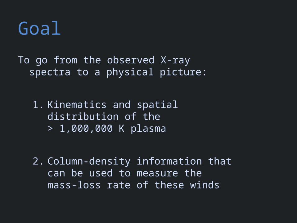
Numerous shock structures, distributed above ~1.5 R*

shock onset at r ~ 1.5 Rstar

Vshock ~ 300 km/s : T ~ 106 K

Shocked wind plasma is decelerated back down to the local CAK wind velocity

The paradigm

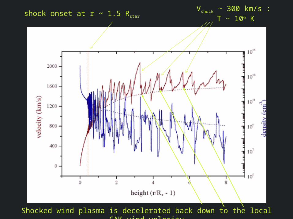
Shock-heated, X-ray emitting plasma is distributed throughout the wind, above some onset radius (Ro)

The bulk of the wind (~99%) is unshocked, cool (T < Teff) and X-ray absorbing (t*)

There are different types of specific models within this paradigm, and many open questions

More realistic 2-D simulations: R-T like break-up; structure on quite small scales

Dessart & Owocki 2003, A&A, 406, L1

Morphology Pup (O4 If)

Capella (G5 III) – coronal source – for comparison

Chandra HETGS (R < 1000) Pup (O4 If)


Morphology – line widths Pup (O4 If)


Ne X Ne IX Fe XVII

Morphology – line widths Pup (O4 If)


Ne X Ne IX Fe XVII

~2000 km/s ~ vinf

Pup (O4 If)

Capella (G5 III) – unresolved

Profile shape assumes beta velocity law and onset radius, Ro

Ro

Rdz'

r'2 (1 R r ')

z

Rdz'

r'2 (1 R r ')

z

Universal property of the wind

z different for each point

Pup (O4 If)

Capella (G5 III) – unresolved

t=1,2,8

key parameters: Ro & t*

M

4Rv

j ~ 2 for r/R* > Ro

= 0 otherwise

Rdz'

r'2 (1 R r ')

z

Ro=1.5

Ro=3

Ro=10

= 1 contours

We fit these x-ray line profile models to each line in the Chandra data

Fe XVIIFe XVII

And find a best-fit t* and Ro…

Fe XVIIFe XVII t* = 2.0

Ro = 1.5

…and place confidence limits on these fitted parameter values

68, 90, 95% confidence limits

Let’s focus on the Ro parameter first

Note that for b = 1, v = 1/3 vinf at 1.5 R*

v = 1/2 vinf at 2 R*

Distribution of Ro values in the Chandra spectrum of z Pup

Consistent with a global Ro = 1.5 R*

Vinf can be constrained by the line fitting too

68% conf. range for fit to these five

points

Vinf from UV (2250 km/s)

Kinematics conclusions

Line widths and shapes are consistent with :

1. X-ray onset radius of ~ 1.5 R*

2. Same b, vinf as the bulk, cold wind

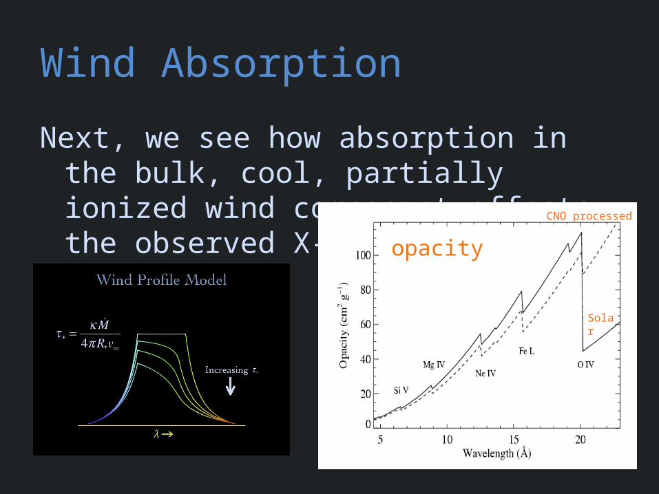
Wind Absorption

Next, we see how absorption in the bulk, cool, partially ionized wind component affects the observed X-rays

CNO processed

Solar

opacity

M

4Rv

opacity of the cold wind wind mass-loss rate

wind terminal velocityradius of the star

€

M•

= 4πr2vρ

t* is the key parameter

describing the absorption

Wind opacity X-ray bandpass

ISM

wind

Wind opacity X-ray bandpass

Chandra HETGS

X-ray opacity CNO processed

Solar

Zoom in

appropriate to z Pup

Opacity is bound-free, inner-shell photoionization

Major ionization edges are labeled

This is the same Fe XVII line we saw a minute ago

Fe XVII

Fe XVII t* = 2.0Ro = 1.5

observer on left

optical depth

contours

t* = 2 in this wind

-0.8vinf

-0.6vinf

-0.2vinf +0.2vi

nf

+0.6vi

nf

+0.8vi

nf

t = 0.3

t = 1

t = 3

Other lines?

Different k – and thus t* – at each wavelength

z Pup: three emission lines

Mg Lya: 8.42 Å Ne Lya: 12.13 Å O Lya: 18.97 Å

t* = 1 t* = 2 t* = 3

Recall:

M

4Rv

Results from the 3 line fits shown previously

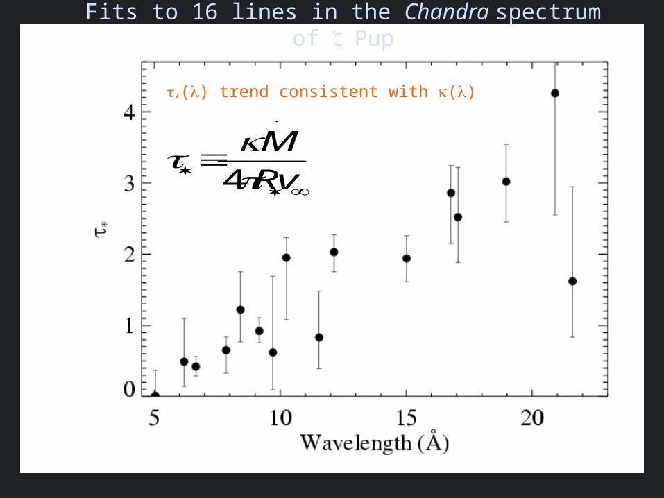
Fits to 16 lines in the Chandra spectrum of zPup


M

4Rv

t*(l) trend consistent with k(l)


Fits to 16 lines in the Chandra spectrum of zPup CNO processed

Solar


M

4Rv

M

4Rv


M becomes the free parameter of the fit to the t*(l) trend

M

4Rv


M becomes the free parameter of the fit to the t*(l) trend

Traditional mass-loss rate: 8.3 X 10-6 Msun/yrFrom Ha ignoring clumping

Our best fit: 3.5 X 10-6 Msun/yr

Fe XVIITraditional mass-loss rate: 8.3 X 10-6 Msun/yr

Our best fit: 3.5 X 10-6 Msun/yr

Mass-loss rate conclusions

The trend of t* value with l is consistent with :

Mass-loss rate of 3.5 X 10-6 Msun/yr

Factor of ~3 reduction w.r.t. unclumped H-alpha

Note: this mass-loss rate diagnostic is a column density diagnostic; it is not a density squared diagnostic and so is not sensitive to clumping (as long as individual clumps are not optically thick).

z Pup mass-loss rate < 4.2 x 10-6 Msun/yr

Implications for broadband X-rays

Pup (O4 If)


Mg XIMg XII

Si XIIISi XIV Ne IX

Ne X H-like vs. He-like

Pup (O4 If)


Mg XIMg XII H-like vs. He-like

Pup (O4 If)


Mg XIMg XII H-like vs. He-like

Spectral energy distribution trendsThe O star has a harder spectrum, but

apparently cooler plasma

This is explained by wind absorption

Wind absorption model

Note that a realistic model of the radiation transport and of the opacity is required to properly account for broadband absorption effects

See Leutenegger et al. 2010 for simple method to incorporate these effects into data analysis

Other stars?

9 Sgr (O4 V)

Lagoon Nebula/M8: Barba, Morrell

9 Sgr (O4 V): t* values

wavelength

t*

M reduction: factor of 6

2.4 X 10-6 to 4 X 10-7

wavelength

Ro

9 Sgr (O4 V): Ro values

Ro = 1.6 R*

Carina: ESO

Tr 14: Chandra

HD 93129A (O2If*) is the 2nd brightest X-ray source in Tr 14

HD93129A – O2 If*

Extremely massive (120 Msun), luminous O star (106.1 Lsun)

Strongest wind of any Galactic O star (2 X 10-5 Msun/yr; vinf = 3200 km/s)

From H-alpha, assuming a smooth

wind

There is an O3.5 companion with a separation of ~100

AU

But the vast majority of the X-rays come from embedded wind shocks

in the O2If* primary

Its X-ray spectrum is hard

H-like vs. He-like

Mg XII Mg XISi XIIISi XIV

Its X-ray spectrum is hard

low H/He

But the plasma temperature is low:little plasma with kT > 8 million K

MgSi

HD 93129A (O2 If*): Mg XII Lya 8.42 Å

Ro = 1.8 R*

t* = 1.4

M-dot ~ 2 x 10-5 Msun/yr from unclumped Ha

Vinf ~ 3200 km/s

M-dot ~ 5 x 10-6 Msun/yr

Low-resolution Chandra CCD spectrum of HD93129AFit: thermal emission with wind + ISM absorption

plus a second thermal component with just ISM

kT = 0.6 keV *wind_abs*ismadd 5% kT = 2.0 keV*ism

kT = 0.6 keV *wind_abs*ismadd 5% kT = 2.0 keV*ism

Typical of O stars like zPup

t*/k = 0.03 (corresp. ~ 5 x 10-6 Msun/yr)

small contribution from colliding wind

shocks

consistent with result from line profile fitting

Approximations and assumptionsExtensively discussed in Cohen et al.

2010

Biggest factors:

bVinf

opacity (due to unc. in metallicity)

Early B (V – III) stars with weak winds

X-ray flux levels in many B star are high considering their low mass-loss rates (known since ROSAT in the 1990s)

Chandra spectroscopy of b Cru (B 0.5 III)

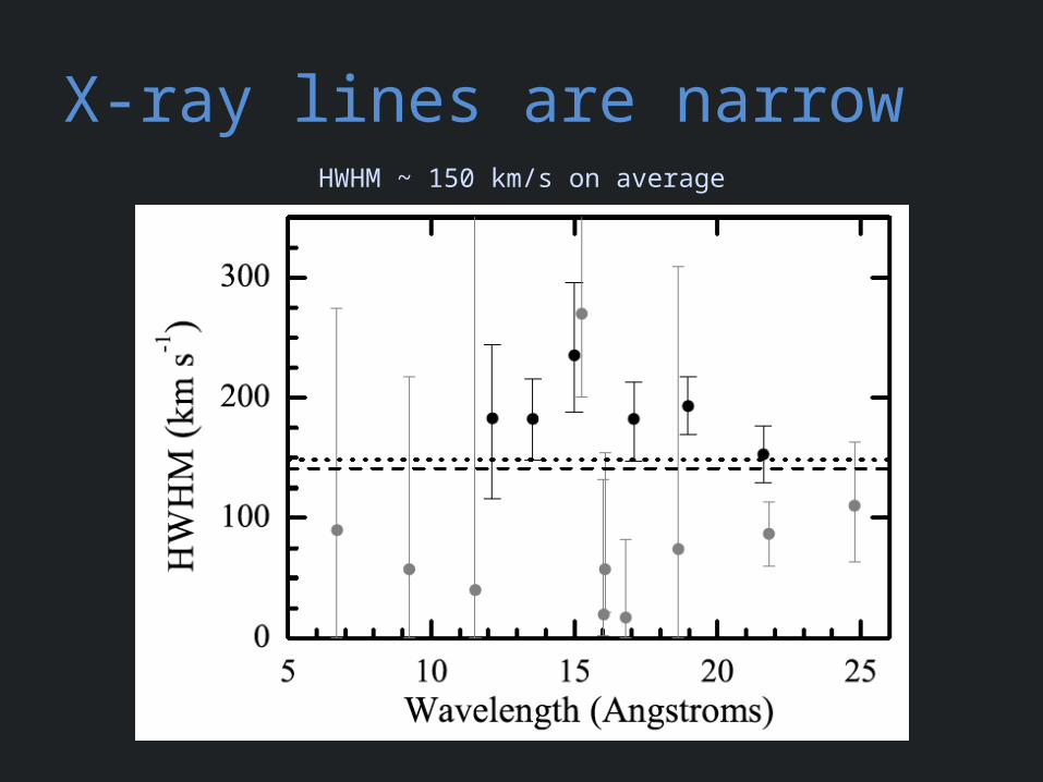
X-ray lines are narrowHWHM ~ 150 km/s on average

Much narrower than expected…From the bulk CAK wind

expectation from CAK wind

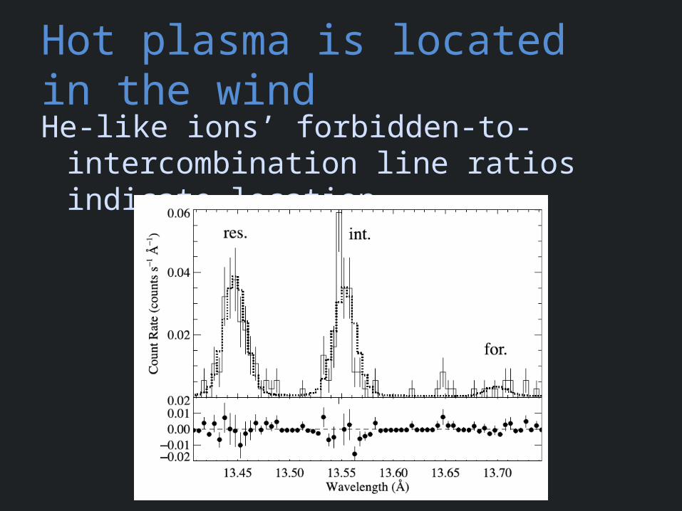
Hot plasma is located in the wind He-like ions’ forbidden-to-

intercombination line ratios indicate location

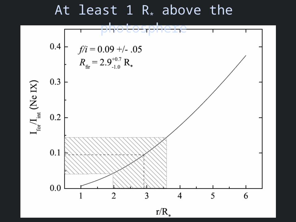
At least 1 R* above the photosphere

B star X-rays are very hard to explain

Lines are not broadBut X-ray plasma is well out in the

wind flowX-ray emission measure requires a

substantial fraction of the wind to be hot (> 106 K)

Conclusions

Single O stars – like z Pup – X-ray line shapes are consistent with kinematics from shock models

And profiles can be used as a clumping-independent mass-loss rate diagnostics

Results are consistent with factor of 3 to 6 reduction over Ha determinations that assume a smooth wind

Conclusions, pt. 2

Broadband wind absorption is measurableIt can significantly harden the observed spectraAnd it, too, is consistent with factor of 3 to 6

reduction over Ha determinations that assume a smooth wind

Even extreme O star winds like HD 93129A’s are consistent with these results

It’s the early B star winds that are hard to understand

Extra Slides

Caveats, reflections

Why did it take so long to identify the wavelength trend?

Realistic opacity modelResonance scatteringPorosity and clumping

Which lines are analyzed?

There are 21 complexes in the Chandra spectrum; we had to exclude 5 due to blending

The short wavelength lines have low S/N, but are very important – leverage on wavelength-dependence of opacity

Seven short wavelength lines never before analyzed

Simplified opacity models are too steep

Oskinova, Feldmeier,Hamann 2006

Detailed opacity model is important

CNO processed

Solar

Realistic opacity is flatter between 12 and 18 Å

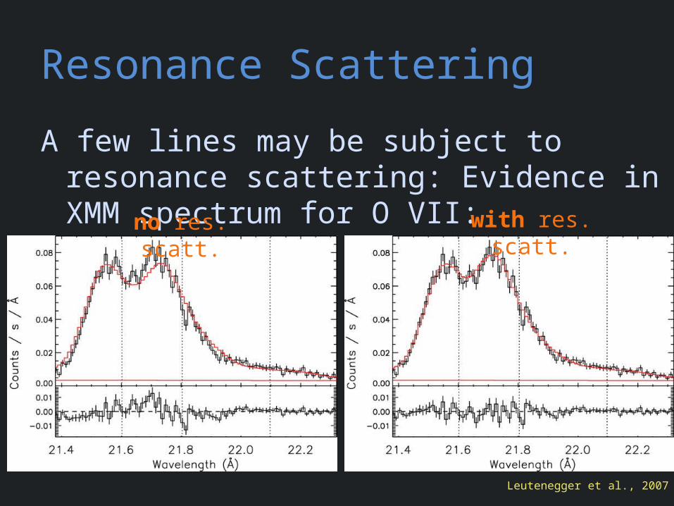
Resonance Scattering

A few lines may be subject to resonance scattering: Evidence in XMM spectrum for O VII:

Leutenegger et al., 2007

no res. scatt. with res. scatt.

What about porosity?

“Clumping” – or micro-clumping: affects density-squared diagnostics; independent of clump size, just depends on clump density contrast

(or filling factor, f )

visualization: R. Townsend

The key parameter is the porosity length,

h = (L3/ℓ2) = ℓ/f

But porosity is associated with optically thick clumps, it acts to reduce the effective opacity of the wind; it does depend on the size

scale of the clumps

L

ℓ

f = ℓ3/L3

Note: whether clumps meet this criterion depends both on the clump properties and on the atomic process/cross-

section under consideration

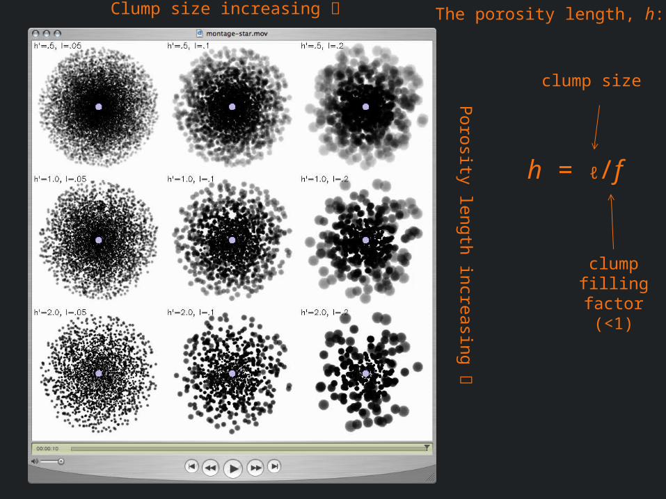
h = ℓ/f

clump size

clump filling

factor (<1)

The porosity length, h:

Poro

sity le

ng

th in

creasin

g

Clump size increasing

Poro

sity le

ng

th in

creasin

g

Clump size increasing

Porous wind

No Porosity

Porosity only affects line profiles if the porosity length (h) exceeds the stellar radius

The clumping in 2-D simulations (density shown below) is on quite small scales

Dessart & Owocki 2003, A&A, 406, L1

No expectation of porosity from simulations

Natural explanation of line profiles without invoking porosity

Finally, to have porosity, you need clumping in the first place, and once you have clumping…you have your factor ~3 reduction in the mass-loss

rate




rate




rate (for z Pup, anyway)

f = 0.1

f = 0.2

f = 0.05

f ~ 0.1 is indicated by Ha, UV, radio

free-free analysis

f = 0.1

f = 0.2

f = 0.05

And lack of evidence for porosity…leads us to

suggest visualization in

upper left is closest to

reality

f = 0.1

f = 0.2

f = 0.05

Though simulations

suggest even smaller-scale

clumping

Incidentally, you can fit the Chandra line profiles with a porous model

But, the fit isn’t as good and it requires a porosity length of 3 R*!

Documents

X-ray Spectral Diagnostics of Activity in O and Early-B Stars wind shocks and mass-loss rates David Cohen Swarthmore College