Grazing incidence SAXS/WAXS using the Pilatus3R 300K detector

on the SAXSLAB instrument

By Charles M. Settens, Ph.D.Center for Materials Science and Engineering at MIT

For assistance in the CMSE X-ray facility contact settens@mit.edu

This SOP and others are available at http://prism.mit.edu/xray/education/downloads.html

The SAXSLAB instrument has the option to be setup to perform grazing incidence small or wide angle X-ray scattering on samples with nanostructured surfaces. Standard training shows how to perform specific alignment for GI-SAXS measurements with uniformly flat thin film samples by using the specularly reflected X-ray beam. After alignment, the sample to detector distance can be changed to probe the length scale of interest; for SAXS (30-2300 Å) for WAXS (3-70 Å).

I. Startup instrument pg 1II. Sample loading procedure pg 1III. Alignment of sample to X-ray beam pg 6IV. Plan and Collect GI-SAXS measurement pg 8V. Writing and Running an automated measurement macro pg 9VI. When You are Done pg 11

Appendix A. Linux operating system pg 11The instrument computer operating system is Ubuntu version 14.04 LTS.

Appendix B. Additional instrument info pg 11-12This section provides additional information about the controlling the drives on the instrument via SPEC commands and Pilatus3R 300K detector information.

Revised 11 July 2016Page 1 of 11

SAXSLAB Operation Checklist

1. Engage the SAXS instrument in Coral Ch I

2. Assess instrument status and safetya. Is the instrument on?b. Is the generator on?c. What is the tube power?d. Is the shutter open?

Ch I

3. Ensure the X-ray tube is at full power 45 kV and 0.66 mA for the Cu microfocus tube Ch I

4. Start the Ganesha System Control software Ch I

5. Start the Ganesha GUI software (Ganesha Interactive Control Center, GICC for short) Ch I

6. Vent SAXS system Ch II

7. Load GISAXS holder with thin film samples Ch II

8. Evacuate SAXS system Ch II

9. Plan GI-SAXS measurements Ch III

10. Align GI-SAXS holder to beam Ch III

11. Write and run and automated measurement macro Ch IV

12. Data reduction with SAXSGUI software Ch V

13. When finisheda. Leave the tube power at full power level:

i. 45 kV and 0.66 mA for the Cu microfocus tubeb. Vent SAXS systemc. Retrieve your sampled. Evacuate SAXS systeme. Clean the sample stage and sample holdersf. Copy your data to a secure locationg. Disengage the SAXS in Coral

Ch VII

The Chapter number and section number on the right-hand side of the page indicate where you can find more detailed instructions in the SAXS SOP.

I. Startup instrument This section walks through starting the SAXS instrument and logging into Coral. The instructions below give some descriptions on how to use the Linux system. If you are not familiar with Linux, read Appendix A.

Revised 11 July 2016Page 2 of 11

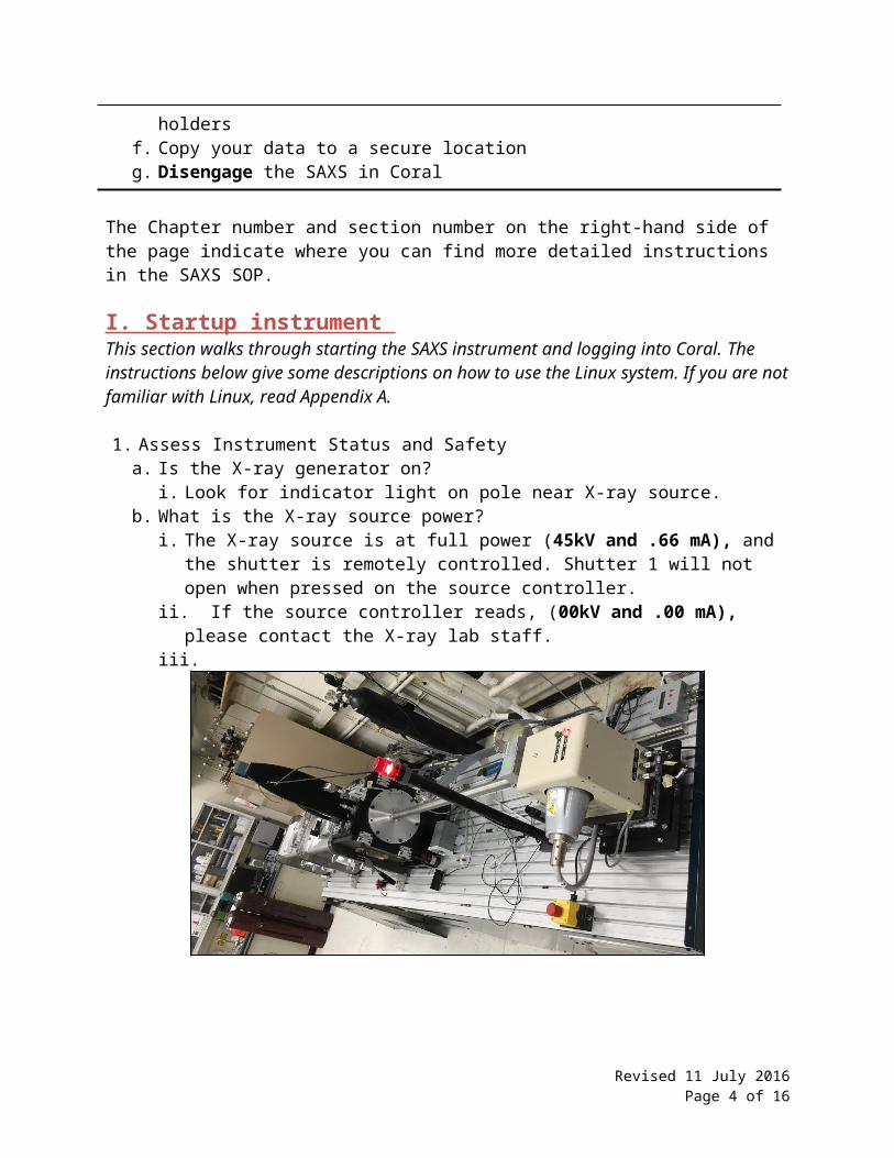
1. Assess Instrument Status and Safetya. Is the X-ray generator on?

i. Look for indicator light on pole near X-ray source.b. What is the X-ray source power?

i. The X-ray source is at full power (45kV and .66 mA), and the shutter is remotely controlled. Shutter 1 will not open when pressed on the source controller.

ii. If the source controller reads, (00kV and .00 mA), please contact the X-ray lab staff.iii.

2. Engage the SAXS system in Coral.

a. Navigate to the Terminal

b. Type: cd /usr/local/coral-remote

c. Type: ./coral-remote-cmse

d. Login to Coral with your username and password

3. Start the programs Ganesha System Control

Revised 11 July 2016Page 3 of 11

a. There are is a toolbar displayed along the bottom of Workspace 1, with the programs that are used to control of the SAXSLAB system labeled SPEC, SL, DET, TVX, GEN, CAM1, GUI, and ED.

b.SPEC: software for instrument control and data acquisition - http://www.certif.com/ SL: server runs on the detector computer and handles processing of the data (cumulative files, includes headers, advanced noise-reduction).DET: server talks directly to the Pilatus3R 300K detectorTVX: server for low level communication to DET serverGEN: server for communication from SPEC to the source generator for opening closing shutter, modifying voltage and current settingsCAM1: software to view samples in chamber via off axis cameraGUI: software for data visualization, image analysis operations and transformations, in-cluding batch mode data reduction and well as basic fitting- http://www.saxsgui.com/ ED: text editor

c. Blue indicates the service is active, Yellow indicates an optional service has been closed and can be reopened by clicking on the toolbar icon, and Red indicates that a critical ser-vice is not running.

d. SAXSGUI will indicate to open an initial image file. i. Open the file: /home/saxslab/SAXSShared/data/latest/ latest_xxxxxxx_craw.tiff

where xxxxxxx is the largest number possible in the directory.ii. Navigate to File > Open latestiii. Select the file: /home/saxslab/SAXSShare/data/latest/latest_xxxxxxx_craw.tiffiv. SAXSGUI now continuously updates as data is acquired. The indicator of this condi-

tion is the red Stop Monitoring button will be enabled at the bottom of the SAXSGUI data visualization screen.

4. Start the Ganesha GUI software (GICC = Ganesha Interactive Control Center).

a. The GICC software has 3 panels, left to right as can be seen below. Left: sample stage graphic control (opened by < button on left of main panel)Center: main control panel (always open)Right: macro editor panel (open by > button on right of main panel)

** Note: If the macro editor panel is OPEN, mouse click the main control and sam-ple stage graphics panel will populate a list of instructions to run in a macro. Close if not intended to make a macro.

Revised 11 July 2016Page 4 of 11

II. Sample loading procedure This section describes the procedure for venting, loading the sample (freestanding or capillary) on the Ambient 8x8 stage and evacuating the system.

1. Vent chamber to load samples.a. In GICC, click the “Vent” button on the bottom right of the main control panel.

i. Dialogue box: Please make sure the sample door is partially unlashed to prevent overpressure. Start venting? Click Start.

b. After 120 seconds of venting the chamber door should be ajar. If this is not the case, click “Vent” button a second time and wait to see that the door opens.

c. Click “Isolate” button to close the valves.

2. Choose the GI-SAXS holder.a. Place samples across the spaces in the GI-SAXS holder.

i. Only the first 3 spaces are available. Spaces are 19mm center to center.

b. Be sure to push holder in to back reference plate. Tighten thumbscrews.

**Only certain spaces in the GISAXS sample holder within the y motor limits (see above).

c. Close chamber door and make sure that the O-ring seal is compressed by pulling up the handle.

3. Record the positions of your samples on the GI-SAXS holder.

Revised 11 July 2016Page 5 of 11

Towardchamberdoor

4. Evacuate SAXS systema. In GICC, click “Evacuate” button on the bottom right of the main control panel.

i. Expect a loud noise as the pump starts.b. The vacuum gauge should read 0.08 mbar after 5 minutes of the chamber evacuating.

III. Alignment of sample to X-ray beam This section describes how to position the sample into the beam and collect alignment measurements.

1. In the SPEC window, type the command a. SPEC> calib_gib. This command moves the

stage to the limit switch in Y and Z and center at the center position 03.

2. In GICC, open Current Holder panel with “>” button on the left of the Main Con-trol panel. a. In the dropdown menu,

choose “GISAXS 19x” holder.

b. Loading “GISAXS 19x” holder with a reference point: Middle-03. Click Go.c. Current Holder graphic is now accurately portraying the actual sample positions.d. Verify that position 03 is Horizontal: 29.590 mm and Vertical 38.700 mm.

3. Use the graphic to move to the desired sample position.

4. Click the “Sample to Beam” button to move the sample into the beam path.c. At the bottom of the Current Holder panel, click the “Sample to Beam” button to move

the sample into the beam path. d. In the Current Holder graphic, the green O should move to the desired position confirm-

ing the translation of the stage.

5. Change the Vertical position of the beam from 38.700 mm to 37.700 mm to ensure that the X-ray beam starts over top of the sample before the automated alignment procedure.

6. At the bottom of the main control panel in Additional Controls, check the “GI SAXS/WAXS box.

7. In Sample Alignment, choose Hybrid Lineup.

Revised 11 July 2016Page 6 of 11

a. This is the automated direct beam half cut alignment procedure that performs a series of successive scans of zsam and thsam in order to align the sample surface to the X-ray beam.

8. A window for SPECplot will automatically open and the entire

active area of the Pilatus detector is summed to a single intensity value as a function zsam, the sample height with respect to the X-ray beam.

9. Zsam is repositioned to the center of mass (COM) of the sample surface. Then, thsam will tilt the sample to find the most paral-lel position over top of the sample. This will happen 2x more times until a well-defined triangular shaped thsam plot is pro-duced about the zero position.

10. In SAXSGUI, navigate to File > Open latesta. Select the file: /home/saxslab/SAXSShare/data/latest/lat-

est_xxxxxxx_craw.tiff where xxxxxxx is the largest num-ber possible in the directory.i. craw files are not corrected for cosmic background radiation.ii. caz files are corrected for cosmic background radiation (in corrected folder).

b. SAXSGUI now continuously updates as data is acquired. The indicator is the Stop Moni-toring button will be enabled.

11. The Hybrid Lineup procedure finishes with 4 detector images at thsam of 0.2, 0.4, 0.6, 0.8 degree tilt angles. The images will display a specular reflection that must be interpreted by the user in order to redefine the zero position of thsam. The scheme is shown below with a sample diagram.

12. In the profile plot in SAXSGUI, hover the cursor over the intensity maxima from the specu-

lar reflection. It reads 2θ = 1.949 degrees, however it should read 1.6 degrees.

13. To redefine the zero position of thsam, divide 2θ by 2. That is, 1.949/2 = 0.9745 degrees.

14. In the GI SAXS/SAXS panela. Redefine = 0.9745 deg (3 decimal places, 0.975 deg).b. Go = 0.8 deg

15. To check the alignment of the specular reflection has indeed been redefined to 2θ = 1.6 de-grees.

Revised 11 July 2016Page 7 of 11

Energy Delta Beta

a. In the Main GICC control panel, in Measurement Details section, take a test measure-ment i. Description: “GI-SAXS alignment 0.8 deg 30sec”ii. Time: 30 seciii. Note down Image number and click Measure button.

IV. Plan and collect GI-SAXS measurement This section describes how to plan GI-SAXS measurements, change configurations and collect GI-SAXS data prior to automated data acquisition. Specific details on how to create and run an automated batch program are covered in sections IV and V.

EXAMPLE IS FOR A POLYETHYLENE POLYMER THIN FILM ON A FLAT SUBSTRATE.

1. What is the intended size you would like to probe?a. SAXS/WAXS measurements are taken as a function on scattering angle, 2θ, from the

forward direction of the radiation. A plot of relative intensity as a function of scattering angle, 2θ assumes the radiation wavelength is known (CuKα1 = 1.5409Å, 8.06 KeV). To normalize the scattering profile to a wavelength independent scale the conversion to, q, the momentum transfer is

q = 4 π sinθ / λ, where θ is ½ the scattering angle and is the λ wavelength in Ångstroms.

q = 2π/d, where d is real space length in units of Å and q is in units of Å-1.

2. In GICC main control panel, select an appropriate Configuration to observe a specific length scale. Options are 2 Apertures WAXS, MAXS, SAXS and ESAXS. Click Go button.

Configuration Name Description detx value

Sample-detector distance

Aperture Sizes

Slit1-Slit2

qmin qmax dmax dmin

0 Open Open Apertures mm mm mm 1/Å 1/Å Å Å

1 WAXS Wide Angle 2mm beamstop 0 109.1 0.9-0.9 0.037 2.06 168 3.05

2 MAXS Medium Angle 2mm beamstop 350 459.1 0.9-0.4 0.009 0.50 706 12.5

3 SAXS Small Angle 2 mm beamstop 950 1059.1 0.7-0.3 0.0039 0.22 1629 28.74 ESAXS Extreme Small Angle 2 mm

bstop1400 1509.1 0.45-0.2 0.0027 0.18 2321 41

Calculated with help from http://www.bio.aps.anl.gov/xraytools.html, assume 172μm pixel size, 8.06keV, Image ra-dius of 330 pixels.

3. Find the Google Chrome Browser, navigate to http://henke.lbl.gov/optical_constants/getdb2.html

4. Enter the chemical formula and mass density for a photon energy of 8000 to 8100 eV (CuKα1 is 8060 eV).a. To request a Text File and Click “Submit

Request.”

Revised 11 July 2016Page 8 of 11

5. A text file will be generated with information of the refractive index in 3 columns.

6. Delta is the real part of the refractive index.

7. To calculate the critical angle for total external reflection, θ c=√2 δ .

a. 2 × 0.0000036529 = 0.0000073058b. √0.000073058=¿0.0027029 radians.c. Change radians to degrees, 0.0027029 × (180/π) = 0.15486 degreesd. θc = 0.15486 degrees

8. To ensure an evanescent wave of X-rays passes along the film surface, choose an angle above the critical angle. a. In the GI SAXS/SAXS panel, Go = 0.12 deg.

9. In the Main GICC control panel, in Measurement Details section, take a test measurementa. Description: “GI-SAXS Sample name 0.12 deg

120sec”b. Time: 120 secc. Note down Image number and click Measure button

10. For well resolved GI-SAXS measurements, collimate the main beam by changing the slit sizes.a. In the GI SAXS/SAXS panel,

i. Primary - Horizontal: 0.3 mm Vertical: 0.3 mmii. Guard – Horizontal: 0.1 mm Vertical: 0.1 mm

11. In the Main GICC control panel, in Measurement Details section, collect a GI-SAXS mea-surement.a. Description: “GI-SAXS Sample name 0.12 deg 600sec”b. Time: 600 secc. Note down Image number and click Measure button

IV. Writing and Running an automated measurement macro This section covers making a macro to automate the data collection at multiple tilt conditions of the sample, detector configurations.

1. Open the right edge of the Main GICC panel for the macro editor with the “>” button.Note: When clicking on any button in the GICC, the action is not performed but instead, writ-ten into the macro list.

a. At the top of the macro editor, click the “New” buttonb. In the GI SAXS/SAXS panel, Go = 0.12 deg.c. In Measurement Details, select a measurement

Revised 11 July 2016Page 9 of 11

ii. Add a description including: sample name, exposure time, hole position, sample thickness

iii. Choose a measurement time in seconds.iv. Click Measure button.

d. Repeat for b and c and increment by 0.1 degrees to a final critical angle value of 0.25 de-grees.

e. Save macros written in the GICC panel with the .gicc extension.

2. If you’d like to insert an instruction in a macro ahead of another without deleting all of the instructions, right click on the instruction and select “Insert before”. The instruction clicked has an anchor icon next to it.

a. Perform mouse clicks on GICC to insert intended action.b. When done adding actions, right click and “Disable insert before”c. Save macros written in the GICC panel with the .gicc extension.

3. Check the sequence of the measurement macro.

4. Click the “Run” button to watch automated collection of the SAXS/WAXS patterns for each sample specified in the macro.

V. Data reduction with SAXSGUI This section walks you through the steps of data reduction with SAXSGUI software from 2D image data to 1D profiles that can then be loaded into standard SAXS data analysis software (SASview).

1. SAXSGUI Basics for output of data:a. Processing > AP with Metadata

i. Select the cosmically corrected .caz files from/home/saxslab/SAXSShared/data/latest

ii. The shared folder to save files:/home/saxslab/SAXSShared/Your folder

b. Data will be outputted in the follow file extensionsi. .grad file (ASCII file with header details)

1. 3 column format (q, I , √ I) orii. .jpg of 1D data from azimuthally averaged 2D

dataiii. .jpg of 2D image with colorbariv. .jpg screenshot of SAXSGUI screen

c. If the SAXSGUI program fails to Autoprocess, Close it and reopen via the SAXSLAB Toolbar.

IV. When you are done This section describes the procedure for venting, loading the sample and evacuating the system.

1. Vent chamber to load samples.

Revised 11 July 2016Page 10 of 11

a. In GICC, click the “Vent” button on the bottom right of the main control panel. i. Dialogue box: Please make sure the sample door is partially unlashed to prevent

overpressure. Start venting? Click Start.b. After 120 seconds of venting the chamber door should be ajar. If this is not the case, click

“Vent” button a second time and wait to see that the door opens

2. Close chamber door and make sure that the O-ring seal is compressed by pulling up the handle.

3. Evacuate SAXS systema. In GICC, click “Evacuate” button on the bottom right of the main control panel.

i. Expect a loud noise as the pump starts.b. The vacuum gauge should read 0.08 mbar after 5 minutes of the chamber evacuating.

4. Logout of Coral.

Appendix A. Linux info The instrument computer operating system is Ubuntu version 14.04 LTS. Tutorials available at http://linuxsurvival.com/

Appendix B. Additional instrument info This section provides additional information about the controlling the drives on the instrument via SPEC commands and Pilatus3R 300K detector information.

Detector info:

Revised 11 July 2016Page 11 of 11