X-MET 880 Field Portable X-Ray Fluorescence Operating - CLU-IN

STANDARD OPERATING PROCEDURES

SOP: 1707

PAGE: 1 of 53

REV: 0.0

DATE: 12/22/94

X-METTM

880 FIELD PORTABLE X-RAY FLUORESCENCE

OPERATING PROCEDURES

CONTENTS

1.0 SCOPE AND APPLICATION

1.1 Principles of Operation

1.1.1 Scattered X-rays

1.2 Sample Types

2.0 METHOD SUMMARY

3.0 SAMPLE PRESERVATION, CONTAINERS, HANDLING AND STORAGE

4.0 INTERFERENCES AND POTENTIAL PROBLEMS

4.1 Sample Placement

4.2 Sample Representivity

4.3 Reference Analysis

4.4 Chemical Matrix Effects (Effects due to the chemical composition of the sample)

4.5 Physical Matrix Effects (Effects due to sample morphology)

4.6 Modeling Error

4.7 Moisture Content

4.8 Cases of Severe X-ray Spectrum Overlaps

4.9 Inappropriate Pure Element Calibration

5.0 EQUIPMENT/APPARATUS

5.1 Description of the X-MET 880 System

5.2 Equipment and Apparatus List

5.2.1 X-MET 880 Analyzer System

5.2.2 Optional Items

5.2.3 Limits and Precautions


SOP: 1707

PAGE: 2 of 53

REV: 0.0

DATE: 12/22/94

X-METTM



CONTENTS (cont)

5.3 Peripheral Devices

5.3.1 Communication Cable Connection

5.3.2 Communication Speed

5.3.3 Character Set

5.3.4 Parity

5.3.5 Terminal Emulation

5.3.6 User Software

5.4 Instrument Maintenance

5.4.1 Probe Window

5.4.2 Further Information and Troubleshooting

6.0 REAGENTS

6.1 Site Specific Calibration Standards (SSCS)

6.1.1 SSCS Sampling

6.1.2 SSCS Preparation

6.2 Site Typical Calibration Standards (STCS)

7.0 PROCEDURE

7.1 Prerequisites

7.1.1 Gain Control

7.1.2 Gain Control Monitoring

7.2 Preoperational Checks

7.3 Normalization and Standardization

7.4 General Keys and Commands

7.4.1 The "Shift" Key

7.4.2 The "Model" (Selection) Key

7.4.3 The "MTIME" (Measurement Time Selection) Key


SOP: 1707

PAGE: 3 of 53

REV: 0.0

DATE: 12/22/94

X-METTM



CONTENTS (cont)

7.4.4 AMS Command: Data Averaging Mode

7.4.5 The "RECALC" Key

7.4.6 The Function Keys "F1 - F5"

7.4.7 STD Command: Standard Deviations

7.4.8 Other Commands

7.5 Instrument Calibration

7.5.1 DEL Command: Deleting a Model

7.5.2 Changing a Model's "Maximum Count Rate" and Default Measuring Time

7.5.3 PUR Command: Pure Element Calibration

7.5.3.1 Introduction

7.5.3.2 Operation

7.5.3.3 Multiple Models

7.5.3.4 LIM Command: Examining and Verifying the Channel Limits

7.5.4 SPE Command: Examining Spectra

7.5.5 SPL Command: Spectrum Plot Using a Peripheral Device

7.5.6 CAL Command: Assay Model Sample Calibration


7.5.6.2 Measurement of Calibration Samples

7.5.6.3 Sample Calibration of a Model Using Both Sources in a DOPS Probe

7.5.6.4 Deletion of the Calibration Intensities Table

7.5.7 ASY Command: Input of Sample Assay Values

7.5.8 MOD Command: Generating the Regression Model

7.5.8.1 Setting the Dependents

7.5.8.2 Setting the Independents

7.5.8.3 Reviewing the Regression Fit Parameters

7.5.8.4 Examining the Residuals Table

7.5.8.5 Deleting Points

7.5.8.6 Examining Coefficients and T Values

7.5.8.7 Reiterating the Model or Exiting


SOP: 1707

PAGE: 4 of 53

REV: 0.0

DATE: 12/22/94

X-METTM



CONTENTS (cont)

7.5.9 Model Optimization Methodology

7.5.9.1 Basic Theory

7.5.9.2 Parameters Used in Regression Modeling

7.5.9.3 Iterative Process of Building the Model

7.5.9.4 Concluding Remarks

7.5.10 Verifying the Accuracy of the Regression Model

7.5.11 Documenting the Regression Model

8.0 CALCULATIONS

9.0 QUALITY ASSURANCE/QUALITY CONTROL

9.1 Precision

9.1.1 Preliminary Detection Limit (DL) and Quantitation Limit (QL)

9.1.2 Field Detection Limit (FDL) and Field Limit of Quantitation (FLOQ)

9.2 Reporting Results

9.3 Accuracy

9.3.1 Additional QA/QC

9.3.2 Matrix Considerations

10.0 DATA VALIDATION

10.1 Active Calibration Model Documentation Method

10.2 Alternate Calibration Model Documentation Method

10.3 Confirmation Samples

10.4 Recording Results

11.0 HEALTH AND SAFETY

12.0 REFERENCES

SUPERCEDES: SOP #1707; Revision 1.0; 11/21/91; U.S. EPA Contract EP-W-09-031..


SOP: 1707

PAGE: 5 of 53

REV: 0.0

DATE: 12/22/94

X-METTM



1.0 SCOPE AND APPLICATION

The purpose of this standard operating procedure (SOP) is to serve as a guide to the start-up, check-out, operation,

calibration, and routine use of the X-Met 880 instrument, for field use in screening of hazardous or potentially

hazardous inorganics. It is not intended to replace or diminish the use of the X-MET 880 Operating Instructions.

The Operating Instructions contain additional helpful information to assist in the optimum instrument utilization

and which form the basis on which new and varying applications can later be based.

The procedures contained herein are general operating procedures which may be changed as required, dependent

on site conditions, equipment limitations, limitations imposed by the QA/QC procedure or other protocol

limitations. In all instances, the ultimate procedures employed should be documented and associated with the final

report.

1.1 Principles of Operation

X-Ray Fluorescence Spectroscopy (XRF) is a nondestructive qualitative and quantitative analytical

technique used to determine the chemical composition of samples. In a source excited XRF analysis,

primary X-rays emitted from a sealed radioisotope source are utilized to irradiate samples. During

interaction of the source X-rays with samples, they may either undergo scattering (dominating process) or

absorption by sample atoms in a process known as the photoelectric effect (absorption coefficient). This

most useful analytical phenomenon originates when incident radiation knocks out an electron from the

innermost shell of an atom. The atom is excited and releases its surplus energy almost instantly by filling

the vacancy created with an electron from one of the higher energy shells. This rearrangement of

electrons is associated with emission of X-rays characteristic (in terms of energy) of the given atom. This

process is referred to as emission of fluorescent X-rays (fluorescent yield). The overall efficiency of the

process described is referred to as excitation efficiency and is proportional to the product of absorption

coefficient and fluorescent yield.

Generally, the X-MET 880 utilizes characteristic X-ray lines originating from the innermost shells of the

atoms, K, L, and occasionally M. The characteristic X-ray lines of the K series are the most energetic

lines for any element and, therefore, are the preferred analytical lines. The K lines are always

accompanied by the L and M lines of the same element. However, being of much lower energy than the K

lines, they can usually be neglected for those elements for which the K lines are analytically useful. For

heavy elements (such as Ce, atomic number (Z)=58, to U, Z=92), the L lines are the preferred lines for X-

MET 880 analysis. The Lα and Lβ lines have almost equal intensities and the choice of one or the other

depends on what interfering lines might be present. A source just energetic enough to excite the L lines

will not excite the K lines of the same element. The M lines will appear together with the L lines.

The X-MET 880 Operating Instructions contain tables that show the energies and relative intensities of

the primary characteristic X-ray lines for all the applicable elements, see Section 1.3.

An X-ray source can excite characteristic X-rays from an element only if the source energy is greater than

the absorption edge energy for the particular line group (i.e., K absorption edge, L absorption edge, M

absorption edge) of the element. The absorption edge energy is somewhat greater than the corresponding

line energy. Actually, the K absorption edge energy is approximately the sum of the K, L and M line


SOP: 1707

PAGE: 6 of 53

REV: 0.0

DATE: 12/22/94

X-METTM



energies, and the L absorption edge energy is approximately the sum of the L and M line energies of the

particular element.

Energies of the characteristic, fluorescent X-rays are converted (within the detector) into a train of electric

pulses, the amplitudes of which are linearly proportional to the energy. An electronic multichannel

analyzer (electronic unit) measures the pulse amplitudes which, since they are proportional to original

energies of emitted characteristic X-rays, are the basis of a qualitative X-ray analysis. The number of

equivalent counts at a given energy is representative of element concentration in a sample basis for

quantitative analysis.

1.1.1 Scattered X-rays

The source radiation is scattered from the sample by two physical reactions: coherent or elastic

scattering (no energy loss) and Compton or inelastic scattering (small energy loss). Thus, the

backscatter (background signal) actually consists of two components with X-ray lines close

together, the higher energy line being equal to the source energy. Since the whole sample takes

part in scattering, the scattered X-rays usually yield the most intense lines in the spectrum. It is

also obvious from the aforementioned that the scattered X-rays have the highest energies in the

spectrum and contribute the most part of the total measured intensity signal.

1.2 Sample Types

Solid and liquid samples can be analyzed for elements Al (aluminum) through U (uranium) with proper

X-ray source selection. Typical environmental applications are:

Heavy metals in soil (in-situ or samples collected from the surface or from bore hole drillings,

etc.), sludges, and liquids (i.e., Pb in gasoline)

Light elements in liquids (i.e., P, S and Cl in organic solutions)

Heavy metals in industrial waste stream effluents

PCB in transformer oil by Cl analysis

Heavy metal air particulates collected on membrane filters, either from personnel samplers or

from high volume samplers.

2.0 METHOD SUMMARY

The X-MET 880 Portable XRF Analyzer employs radioactive isotopes, such as Fe-55, Cm-244, Cd-109 and Am-

241 for the production of primary X-rays. Each source emits a specific energy range of primary X-rays that cause a

corresponding range of elements in a sample to produce fluorescent X-rays. When more than one source can excite

the elements of interest, the appropriate source(s) is selected according to its excitation efficiency for the elements

of interest. See X-MET 880 Operating Instructions for a chart of source type versus element range, Section 1.17.

For measurement, the sample is positioned in front of the source-detector window and exposed to the primary


SOP: 1707

PAGE: 7 of 53

REV: 0.0

DATE: 12/22/94

X-METTM



(source) X-rays by pulling a trigger on the probe (or pushing the top of the probe unit back on the sample type

probe) which exposes the sample to radiation from the source. The sample fluorescent and backscattered X-rays

enter through the beryllium (Be) detector window and are detected in the active volume of a high-resolution, gas-

filled proportional counter.

Elemental count rates (number of net element pulses per second) are used in correlation with actual sample

compositions to generate calibration models for qualitative and quantitative measurements.

Analysis time is user selectable from 1 to 32767 seconds. The shorter measurement times (30 - 100s) are generally

used for initial screening and hot spot delineation, while longer measurement times (100 - 500s) are typically used

for higher precision and accuracy requirements.

3.0 SAMPLE PRESERVATION, CONTAINERS, HANDLING AND STORAGE

This SOP specifically describes equipment operating procedures for the X-MET 880; hence, this section is not

applicable to this SOP.

4.0 INTERFERENCES AND POTENTIAL PROBLEMS

The total error of XRF analysis is defined as the square root of the sum of squares of both instrument precision and

user or application related error. Generally, the instrument precision is the least significant source of error in XRF

analysis. User or application related error is generally the more significant source of error and will vary with each

site and method used. The components of the user or application related errors are the following:

4.1 Sample Placement

This is a potential source of error since the X-ray signal decreases as you increase the distance from the

radioactive source. However, this error is minimized by maintaining the same sample distance from the

source.

4.2 Sample Representivity

This can be a major source of error if the sample and/or the site-specific or site-typical calibration

samples (see Section 4.0) are not representative of the site. Representivity is affected by the soil macro-

and micro-heterogencity. For example, a site contaminated with pieces of slag dumped about by a

smelting operation will be less homogeneous than a site contaminated by liquid plating waste. This error

can be minimized by either homogenizing a large volume of sample prior to analyzing an aliquot, or by

analyzing several samples (in-situ) at each sampling point and averaging the results.

4.3 Reference Analysis

Soil chemical and physical matrix effects may be corrected by using Inductively-Coupled Plasma (ICP) or

Atomic Absorption (AA) spectrometer analyzed site-specific soil samples as calibration samples. A

major source of error can result if the samples analyzed are not representative of the site and/or the

analytical error is large. With XRF calibrations based on reference analyses results, the XRF analytical

results can be reported in the same units as the calibration samples reference analyses. Results, for


SOP: 1707

PAGE: 8 of 53

REV: 0.0

DATE: 12/22/94

X-METTM



example, will be in Contract Laboratory Protocol (CLP) extractable metals if the CLP specified

HNO3/H2O2 digestion is used. Results will be in total metals if total (HF) digestion or KOH fusion is

used.

4.4 Chemical Matrix Effects (Effects due to the chemical composition of the sample)

Chemical matrix effects result from differences in concentrations of interfering elements. These effects

appear as either spectral interferences (peak overlaps) or as X-ray absorption/enhancement phenomena.

Both effects are common in soils contaminated with heavy metals. For example, Fe (iron) tends to absorb

Cu (copper) K shell X-rays, reducing the intensity of Cu measured by the detector. This effect can be

corrected if the relationship between Fe absorption and the Cu X-ray intensities can be modeled

mathematically. Obviously, establishing all chemical matrix relationships during the time of instrument

calibration is critical. These relationships are modeled mathematically, with X-MET 880 internal

software, using ICP or AA analyzed site-specific soil samples as the XRF calibration standards.

Additionally, increasing the number of standards and the range of the standard concentrations used may

decrease the error in the calibration mathematical modeling. Generally, as rule-of-thumb, a minimum of

five calibration samples per element to be analyzed are used to generate reliable X-MET 880 calibration

models.

4.5 Physical Matrix Effects (Effects due to sample morphology)

Physical matrix effects are the result of variations in the physical character of the sample. They may

include such parameters as particle size, uniformity, homogeneity and surface condition. For example,

consider a sample in which the analyte exists in the form of very fine particles within a matrix composed

of much courser material. If two separate aliquots of the sample are ground in such a way that the matrix

particles in one are much larger than in the other, then the relative volume of analyte occupied by the

analyte-containing particles will be different in each. When measured, a larger amount of the analyte will

be exposed to the source X-rays in the sample containing finer matrix particles; this results in a higher

intensity reading for that sample and, consequently, in apparently higher measured concentration of that

element.

4.6 Modeling Error

The error in the calibration mathematical modeling is insignificant (relative to the other sources of error)

IF the instrument's modeling operating instructions are followed correctly (see Section 14.0).

4.7 Moisture Content

If measurement of soils or sludges is intended, the sample moisture content will affect the accuracy of the

analysis. The overall error from moisture may be a secondary source of error when the moisture range is

small (5-20%), or may be a major source of error when measuring on the surface of soils that are

saturated with water.

4.8 Cases of Severe X-ray Spectrum Overlaps

Certain X-ray lines from different elements, when present in the sample, can be very close in energy and,


SOP: 1707

PAGE: 9 of 53

REV: 0.0

DATE: 12/22/94

X-METTM



therefore, interfere by producing a severely overlapped spectrum.

The typical spectral overlaps are caused by the Kβ line of element Z-1 (or as with heavier elements, Z-2 or

Z-3) overlapping with the Kα line of element Z line. This is the so-called Kα/Kβ interference. Since the

Kα:Kβ intensity ratio for the given element usually varies from 5:1 to 7:1, the interfering element, (Z-1),

must be present in large concentrations in order to disturb the measurement of analyte Z. The presence of

large concentrations of titanium (Ti) could disturb the measurement of chromium (Cr). The TiKα and Kβ

energies are 4.51 and 4.93 Kev, respectively. The CrKα energy is 5.41 Kev. The resolution of the detector

is approximately 850 eV. Therefore, large amounts of Ti in a sample will result in spectral overlap of the

TiKβ with the CrKα peak.

Other interferences are K/L, K/M and L/M. While these are less common, the following are examples of a

severe overlap:

AsKα/PbLα , SKα/PbMα

In the arsenic/lead case, lead can be measured from the PbLβ line, and arsenic from either the AsKα or the

AsKβ line; this way the unwanted interference can be corrected. However, due to the severances of the

overlap (energy of AsKα is almost identical to that of PbLα), measurement sensitivity is reduced.

4.9 Inappropriate Pure Element Calibration

It is of paramount importance that the pure element calibration, also called "instrument calibration" (see

Section 12.0), include all elements that can be present at the site, (i.e., in the samples to be analyzed).

This means that even if the element is not a target element, as long as it is present in detectable amounts

with the source in use, it must be included in the pure element calibration in order for the X-MET 880 to

correct for its potential spectral interference effect on the target element.

5.0 EQUIPMENT/APPARATUS

5.1 Description of the X-Met 880 System

The X-MET 880 analyzer includes a compact, sealed radiation source contained that is in a measuring

probe. This probe is connected by cable to an environmentally sealed electronic module.

The analyzer utilizes the method of Energy Dispersive X-Ray Fluorescence (EDXRF) spectrometry to

determine the elemental composition of soils, sludges, aqueous solutions, oils, and other waste materials.

Each probe is equipped with a high resolution gas-filled proportional detector, or a high resolution solid

state lithium drifted silicon (Si/Li) detector.

The complete X-MET 880 system consists of five alternate configurations.

1. The X-MET 880ES Extended Range X-MET 880 Silicon Detector System includes the Silicon

Detector Surface Probe System (SDPS) with a 60 millicurie (mCi) Curium-244* (Cm-244)

excitation source and a 30 mCi Americium-241** (Am-241) excitation source.


SOP: 1707

PAGE: 10 of 53

REV: 0.0

DATE: 12/22/94

X-METTM



2. The X-MET 880SH, Standard X-MET 880 System comes with a SAPS probe containing a 60

mCi Cm-244* excitation source.

3. The X-MET 880ER Extended Range X-MET 880 System comes with a DOPS probe that

contains a 60 mCi Cm-244* excitation source and a 30 mCi Am-241** excitation source.

4. The X-MET 880AS Alternate Standard Range X-MET 880 System comes with a SAPS probe

containing 10 mCi Cd-109*** (in place of the 60 mCi Cm-244).

5. The X-MET 880AE Alternate Extended Range X-MET 880 System includes the DOPS with 10

mCi Cd-109*** plus 30 mCi Am-241**.

* Cm-244 in SDPS probe (or Surface Analysis Probe Set (SAPS) and Double Source Surface

Probe Set (DOPS) probes) will allow analysis of all elements from atomic number 19

(potassium) to 35 (bromine) and from atomic number 56 (barium) to atomic number 83

(bismuth).

** The Am-241 excitation source extends the elemental range of the system to include such

important priority pollutants as Cd, Ag, and Ba. Am-241 in SDPS, SAPS or DOPS will allow

analysis of all elements from atomic number 30 (zinc) to 60 (neodymium), and atomic number

73 (tantalum) to 92 (uranium).

*** Replacing the Cm-244 with Cd-109 provides somewhat improved precision and accuracy for

Pb when As is present. Cd-109 in SAPS or DOPS will allow analysis of elements from atomic

number 24 (chromium) to 42 (molybdenum) and from 65 (terbium) to 92 (uranium).

Optional sample type probes (for laboratory or mobile lab use only) are available for use when all

samples will be contained in X-ray cups. These probes can contain any of the excitation sources

described above.

The use of the special optional sample probes, Light Element sample Probe System (LEPS), or the

Surface Light element Probe System (SLPS), with the Fe-55 ring source, enables analysis of light

elements ranging from atomic number 13 (aluminum), to atomic number 24 (chromium), and heavy

elements from 37 (rubidium) to 56 (barium).

The electronic module includes a 256 channel multi-channel analyzer and a high speed, 16/32 bit,

Motorola 68000 microprocessor. Up to 32 multi-element analysis programs, called models, can be stored

in its memory.

The unit comes factory pre-calibrated based on the Outokumpu Electronics synthetic soil calibration suite,

or based on customer supplied standards (see supplemental documentation on factory calibration for

calibration data specific to each X-MET 880).

Optional calibrations can be installed at the factory for other soil or waste material types on request.


SOP: 1707

PAGE: 11 of 53

REV: 0.0

DATE: 12/22/94

X-METTM



Additional models tailored to specific needs may be added by the user after attending the X-MET 880

Calibration and Operators Training Course which is conducted by Ouotkumpu Electronics at regular

intervals. (Request course description and schedule from Outokumpu Electronics, Langhorne, PA.)

The X-MET 880 can be operated from a 115-volt (or 220-volt) wall outlet or its 12-volt, 10-hour

capacity battery, or a standard 12-volt car or truck battery.

The X-MET 880 can be operated in a temperature range from 32 to 1400 Fahrenheit (F), or may be

operated down to -130 F with the low temperature option. The freezing point of a discharged battery is

140 F.

The probe and electronic unit may be exposed to a light rain. However, additional protection is provided

if the system (electronic unit and probe) is contained in the optional water repellant carrying case.

The instrument can be calibrated for up to 10 elements per model, six (6 target elements) of which can

provide a readout in the Assay Mode.

In the Assay Mode, up to 30 reference samples per assay model can be used to generate the sample

calibration curve in the X-MET 880.

5.2 Equipment and Apparatus List

5.2.1 X-MET 880 Analyzer System

The complete X-MET 880 Analyzer System includes:

880 Electronics Module

Single source SAPS or DOPS or SDPS with optional LEPS or optional Heavy

Element Sample Probe Set (HEPS) in place of, or in addition to, the SAPS and/or

DOPS, each containing appropriate excitation source(s)

Pure element standards

Battery charger

Battery pack

X-MET 880 Operating Instructions, X-MET 880 Operator's Manual and any

applicable X-MET 880 factory calibration documentation.

5.2.2 Optional Items

31 millimeter (mm) diameter sample cups


SOP: 1707

PAGE: 12 of 53

REV: 0.0

DATE: 12/22/94

X-METTM



XRF polypropylene film, 0.2mm thickness

Nylon reinforced, water-repellant backpack

Metal reinforced shipping case with die-cut foam inserts for X-MET 880 and

accessories

Peripheral devices such as the Terminal/Printer data logger, the DMS-1 Data

Management System, the ESP extended software package for use with IBM

compatible Personal Computer (PC).

Surface probe shield assembly. Shield assembly must be used when the SAPS or

DOPS probes are inverted for measuring sample in XRF cups.

See Outokumpu Electronics X-MET 880 Accessories Price List for additional Outokumpu

Electronics options.

For mobile lab or laboratory X-ray sample preparation accessories, such as drying ovens,

grinders, sieves, etc., consult general laboratory equipment suppliers.

5.2.3 Limits and Precautions

The probes should be handled in accordance with the following radiological control practices:

1. The probe should always be in contact with the surface of the material being analyzed

and the analyzed material should completely cover the probe opening (aperture),

when the probe shutter is open. The indicator flag on the side of the DOPS and SAPS

probes is green when the shutter is closed and red when it is open.

2. Under no circumstances should the probe be pointed at the operator or surrounding

personnel with the shutter open.

3. Do not place any part of the operator's or co-worker's body in line of exposure when

the shutter is opened and not fully covered.

4. The SAPS or DOPS probe trigger must be key-locked when not in use.

5. Notify Outokumpu Electronics immediately of any condition or concern relative to the

probe structural integrity, source shielding, shutter condition or operability.

6. Notify the appropriate state agency or Nuclear Regulatory Commission (NRC) office

(see factory supplied data on radiological safety) immediately of any damage to the

radioactive source, or any loss or theft of the device.

7. Labels or instructions on the probe(s) must not be altered or removed.


SOP: 1707

PAGE: 13 of 53

REV: 0.0

DATE: 12/22/94

X-METTM



8. The user must not remove the probe covers or attempt to open the probe.

9. The source(s) in the probe must be leak tested every six (6) months as described in the

X-MET 880 Operating Instructions. The Leak Test Certificates must be kept on file

and a copy must accompany the instrument at all times.

10. The probe shield assembly must be used when the SAPS or DOPS probe is inverted

for measuring samples contained in cups.

11. During operation, keep the probe at least 10 feet from computer monitors and any

other source of radio frequency (RF). Some monitors have very poor RF shielding and

will affect measurement results.

12. The X-MET 880 should not be dropped or exposed to conditions of excessive shock

or vibration.

13. Keep the force on the probe, with the trigger pulled, to less than four (4) pounds to

avoid shutter binding.

Additional precautions include:

1. Do not pull on the probe wire to unplug the probe. Grasp the probe plug at the ribbed

rubber connector cover and squeeze, then press firmly while plugging, and pull while

unplugging the connector.

2. Do not attempt to rotate the handle on the electronic unit unless the release buttons on

each side of the handle are depressed.

3. The X-MET 880 should not be operated or stored at an ambient temperature below

320F (-13

0F with low temperature version) or above 140

0 F.

4. The battery charging unit should only be used indoors at dry conditions.

5.3 Peripheral Devices

The X-MET 880 may be used with a wide range of peripheral devices for electronic data capture or

printed readout as long as they are equipped with input compatible with the RS-232 serial protocol. Such

devices include terminals, printers, electronic data loggers, personal computers, etc. Any time a

peripheral device is connected to the X-MET 880, all text and commands shown on the X-MET 880

display will be automatically output to and copied by the peripheral.

5.3.1 Communication Cable Connection

Plug the round connector of the RS-232 cable, into the X-MET 880 "IN/OUT" port (the

connection just above the probe connection on the electronic unit), and the rectangular (25 pin)

connector of the cable to the RS-232 port of the receiving device (serial port).


SOP: 1707

PAGE: 14 of 53

REV: 0.0

DATE: 12/22/94

X-METTM



If the receiving device, serial port, does not have a 25 pin, male, RS-232 C standard connector,

THEN it will be necessary to obtain a "gender mender plug" (male-to-female converter), OR, in

the case of 9 pin device connectors, a 25 to 9 pin adapter (with or without gender changer,

depending on the gender of the connector at the receiving device). All Outokumpu supplied

peripherals are delivered with appropriate connections.

5.3.2 Communication Speed

To communicate with the external device, the X-MET 880 MUST be set at the same Baud Rate

as the receiving device. The X-MET 880 command for setting or resetting the Baud Rate is CSI

(Configure Serial Interface). The CSI command is a sub-command under the EMP (Enter

Maintenance Parameters) command, which must therefore precede it. Enter EMP followed by

"CONT/YES", THEN enter CSI on the keypad FOLLOWED by "CONT/YES". The X-MET

880 will display

BAUD RATE: XXXX NEW?

Press "CONT/YES" until the desired baud rate (data transfer speed) is in the display, then press

"END/NO" to accept the displayed reading. The baud rate can have values 50, 75, 110, 134.5,

150, 200, 300, 600, 1200, 1800, 2400, 4800, 9600 and 19200 baud. Select the baud rate of the

peripheral device with which you are communicating.

5.3.3 Character Set

The RS-232 C interface supports all the standard ASCII characters. Upper and lower case

letters are equivalent in data transmission. This means that the X-MET 880 will execute any

legal command typed in lower case on the peripheral keyboard. (See Section 5.3.5 for some

special keys.) The serial data format is:

* 1 start bit (SPACE)

* 8 data bits (ASCII from LSB to MSB)

* 1 stop bit (MARK)

5.3.4 Parity

Parity MUST be set to NO PARITY.

5.3.5 Terminal Emulation

Although most keys on the standard typewriter style keypad (as used on most terminals and

computers) are the same as the X-MET 880 keypad, there are, however, some specific keys on

the X-MET 880 that require the operator to use an "equivalent" key on the terminal. The

following lists correlates the unique X-MET 880 keys and their terminal equivalents:

X-MET 880 KEY TERMINAL KEY (or key combination)


SOP: 1707

PAGE: 15 of 53

REV: 0.0

DATE: 12/22/94

X-METTM



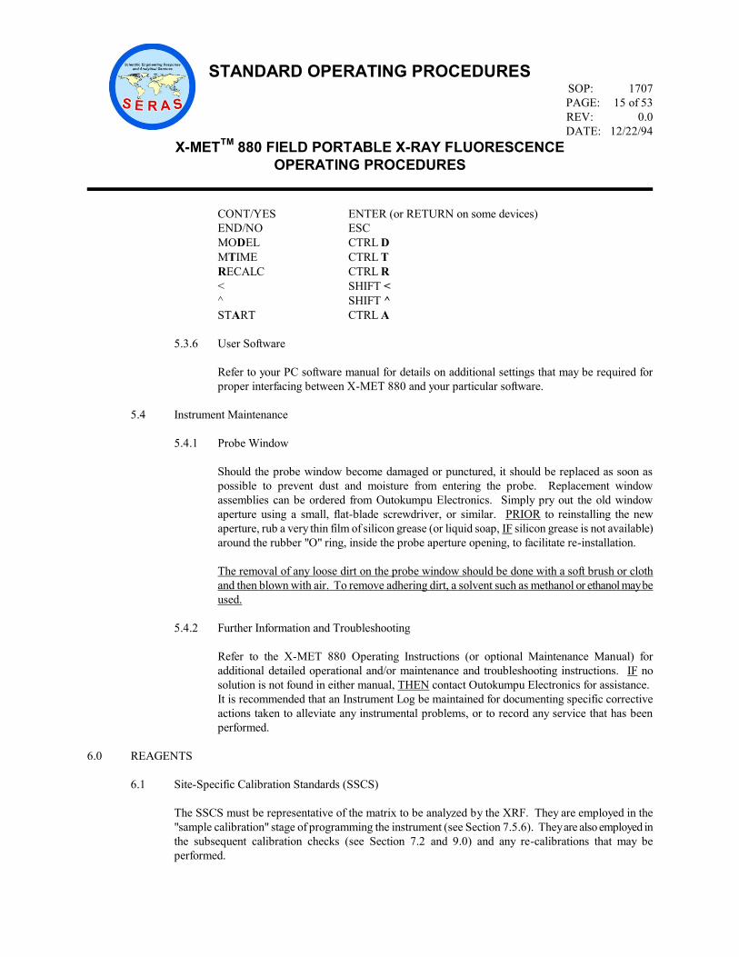
CONT/YES ENTER (or RETURN on some devices)

END/NO ESC

MODEL CTRL D

MTIME CTRL T

RECALC CTRL R

< SHIFT <

^ SHIFT ^

START CTRL A

5.3.6 User Software

Refer to your PC software manual for details on additional settings that may be required for

proper interfacing between X-MET 880 and your particular software.

5.4 Instrument Maintenance

5.4.1 Probe Window

Should the probe window become damaged or punctured, it should be replaced as soon as

possible to prevent dust and moisture from entering the probe. Replacement window

assemblies can be ordered from Outokumpu Electronics. Simply pry out the old window

aperture using a small, flat-blade screwdriver, or similar. PRIOR to reinstalling the new

aperture, rub a very thin film of silicon grease (or liquid soap, IF silicon grease is not available)

around the rubber "O" ring, inside the probe aperture opening, to facilitate re-installation.

The removal of any loose dirt on the probe window should be done with a soft brush or cloth

and then blown with air. To remove adhering dirt, a solvent such as methanol or ethanol may be

used.

5.4.2 Further Information and Troubleshooting

Refer to the X-MET 880 Operating Instructions (or optional Maintenance Manual) for

additional detailed operational and/or maintenance and troubleshooting instructions. IF no

solution is not found in either manual, THEN contact Outokumpu Electronics for assistance.

It is recommended that an Instrument Log be maintained for documenting specific corrective

actions taken to alleviate any instrumental problems, or to record any service that has been

performed.

6.0 REAGENTS

6.1 Site-Specific Calibration Standards (SSCS)

The SSCS must be representative of the matrix to be analyzed by the XRF. They are employed in the

"sample calibration" stage of programming the instrument (see Section 7.5.6). They are also employed in

the subsequent calibration checks (see Section 7.2 and 9.0) and any re-calibrations that may be

performed.


SOP: 1707

PAGE: 16 of 53

REV: 0.0

DATE: 12/22/94

X-METTM



The concentration of the target elements in the SSCS should be determined by independent AA or ICP

analysis that meets an acceptable quality for referee data.

Additionally, the concentration in the SSCS of elements adjacent (+/-2 atomic numbers Z) to the Z of the

target element should be determined by independent AA or ICP analysis if: 1) they are excited by the

source used, and/or 2) their concentrations are unknown or suspected to be greater than ten percent of the

target element concentration and/or 3) it is unknown or suspected that their concentration variance is

greater than twenty percent in the site matrix, or if this variance (if greater than twenty percent) has a non-

linear relationship to the variance of the target element concentration.

For example, the requested target elements are Cd and Sb for a site. Review of the site history indicates

that Sn and Ag may be present. The SSCS should be analyzed for Sn and Ag in addition to Cd and Sb, to

determine their concentrations and the relationship (linear or non-linear) to the Cd and Sb concentrations

in the SSCS samples.

6.1.1 SSCS Sampling

Review Section 4.2 on sample representivity. The SSCS samples must be representative of the

matrix to be analyzed by XRF. It does not make sense to collect the SSCS samples in the site

containment area if you are interested in investigating off-site contaminant migration. The

matrices may be different and could affect the accuracy of the XRF results. If there are two

different matrices on-site, collect two sets of SSCS samples.

A full range of target element concentrations is needed to provide a representative calibration

curve. Mixing high and low concentration soils to provide a full range of target element

concentrations is not recommended due to homogenization problems. The highest and lowest

SSCS samples will determine the linear calibration range. Unlike liquid samples, solid samples

cannot be diluted and re-analyzed.

The number of SSCS samples needed for calibrating an assay model depends on:

1. The number of target elements (analyte). For each additional target element, increase

the number of SSCS samples by five (up to a maximum of 30).

2. The number of elements adjacent to the target elements. For each additional adjacent

element known or found to be present in the samples, you should increase the number

of SSCS samples by five (up to a maximum of 30) to insure that the calibration model

properly corrects for X-ray interferences and spectral overlaps.

Additionally, collect several SSCS samples in the concentration range of interest. If the action

level of the site is 500 mg/kg, providing several SSCS samples in this concentration range will

tend to improve the XRF analytical accuracy in this concentration range.

Generally, a minimum of 10 and a maximum of 30 appropriate SSCS samples should be taken.

A minimum of a 4 oz. sample is required. A larger size sample should be provided to


SOP: 1707

PAGE: 17 of 53

REV: 0.0

DATE: 12/22/94

X-METTM



compensate for samples with a greater content of non-representative material such as rocks

and/or organic debris. Standard glass sampling jars should be used.

6.1.2 SSCS Preparation

The SSCS samples should be dried either by air drying overnight, or oven drying at less than

105 C. Aluminum drying pans or large plastic weighing boats for air drying may be used. After

drying, remove all large organic debris and non-representative material (twigs, leaves, roots,

insects, asphalt, rocks, etc.).

The sample should be sieved through a 20-mesh stainless steel sieve. Clumps of soil and sludge

should be broken up against the sieve using a stainless steel spoon. Pebbles and organic matter

remaining in the sieve should be discarded. The under-sieve fraction of the material constitutes

a sample.

Although a maximum final particle size of 20-mesh is normally recommended, a smaller particle

size may be desired (see Section 4.5). The sample should be homogenized by dividing the

sieved soil into quarters and physically mixing opposite quarters with a clean stainless steel

spoon. Re-composite and then repeat the quartering and mixing procedure three times. Place

the sieved sample in a clean glass sample jar and label it using both the site name and sample

identification information.

The stainless steel sieves should be decontaminated using soap and water and dried between

samples.

One or more plastic XRF sample cups should be filled with the sieved soil for each SSCS

sample. A piece of .2mm polypropylene film is cut and tensioned, wrinkle-free, over the top of

the x-ray sample cup and then sealed using the plastic film securing ring. The cup should be

labeled using both the site name and specimen identification information.

Either the XRF sample cup or the balance of the prepared sample is submitted to the approved

laboratory for analysis of the requested element(s) by AA or ICP.

6.2 Site Typical Calibration Standards (STCS)

When the goal of the analysis with X-MET 880 is semi-quantitative measurements, such as hot spot

delineation or determination of sampling points for a SSCS, then use of a STCS may be the most

appropriate method. STCS are SSCS from a different site that have the identical target elements in a

similar range and matrix as the site that is to be analyzed. It should be noted that the STCS are not from

the site to be analyzed and may generate false positive and negative results.

For example, samples are going to be taken at lead battery manufacturing site for a SSCS. There is no

information in the site history on the location or concentration of the Pb contamination. A model

calibrated for Pb with a SSCS from another battery breakage site could be used as a STCS to screen this

site and locate low, mid and high Pb contamination points for the SSCS sampling.


SOP: 1707

PAGE: 18 of 53

REV: 0.0

DATE: 12/22/94

X-METTM



7.0 PROCEDURE

7.1 Prerequisites

If the X-MET 880 will be used in a location where AC power outlets are conveniently accessible, connect

the battery charger to the battery and plug the charger cord into the outlet. The cable probe must be

connected before the power is switched on. Plugging and unplugging this cable with the power on can

damage the detector.

Verify that the probe shutter is closed by checking the mechanical flag color on the side of the SAPS or

DOPS. When the flag is green the shutter is closed and open when it is red.

Connect the probe cable to the connector labeled "PROBE" on the electronic module. Make certain the

plug has been firmly pushed in all the way (you will feel and hear a slight "click" as the probe connector

locks into position).

Apply power to the X-MET 880 by pressing the "ON" button.

Verify that the display briefly reads:

X-MET 880 VX.X.X (software version) and DATE

SELF TEST COMPLETED, followed by (if the X-MET 880 has been off, more than a few minutes) the

message:

GAIN CONTROL: COUNT RATE TOO LOW

will flash intermittently (along with a "beep") on the display. This is normal and will stop approximately

30 seconds after power is on.

Verify that a prompt sign (>) appears in the lower left corner of the display after the gain control message

has stopped flashing.

Verify that the upper right corner of the display reads the number of seconds (0 - 32,000s) on the top line

and the model number (1 - 32) on the bottom line.

If a "battery low" message appears recharge the battery before proceeding or operate using line voltage.

Allow the X-MET 880 to warm up for approximately 60 minutes.

If the X-MET 880 is being used in a location where the temperature of the environment has changed by

more than 5oF, then allow the X-MET 880 to stabilize at the new ambient temperature. Approximately 1

minute stabilization time for each 1oF change in ambient temperature should be allowed.

7.1.1 Gain Control


SOP: 1707

PAGE: 19 of 53

REV: 0.0

DATE: 12/22/94

X-METTM



Allow 5 minutes after temperature stabilization for the X-MET 880 to perform a complete cycle

of automatic electronic gain control. The trigger must be released on the probe to activate the

gain control operation. Additionally, the prompt sign (>) must be in the display.

The X-ray spectrum contains a number of incident X-ray quantum energies of which there are

corresponding channels in the multichannel analyzer. These channels are limited by certain

changes in conditions such as the resolution of the detector and temperature coefficients. This

means that a proportionally large error from measurement would be obtained, if no

compensation was made for these variations.

The elimination of such errors is made possible by monitoring the state of the probe spectrum

and compensating for any spectral drift as described in Section 7.1.2.

The state of the detection region is maintained by a feedback gain control system, which

operates all the time the probe is in a non-operative position (gain control position, DOPS,

SAPS, SLPS placed on their sides, HEPS, LEPS with the lid in the forward position) and the

instrument is not under any command (i.e., prompt displayed (> )).

The gain control routine is accomplished by allowing the X-MET 880 to measure a reference

material (usually copper) mounted on the shutter and then maintaining a track on the peak

spectral position.

The initial peak position is set up during the initialization of the probe (INI) and from this point

the instrument will adjust accordingly, during gain control.

7.1.2 Gain Control Monitoring

During initialization, the initial peak channel is established for the gain control. During gain

control, adjustments are made to return the maximum peak (usually copper), after the

backscatter peak, to this initial peak channel location. The peak channel is monitored and

recorded to verify if the gain control mechanism is working and returning the peak to the correct

channel. Failure of the gain control mechanism will result in spectral drift and calculation of

incorrect intensities in the element windows or incorrect pure element window calibration. The

gain control peak channel should be measured and recorded at the beginning, end, and every 25

to 40 minutes during the following operations:

1. Pure element calibration

2. SSCS Measurements

3. All sample analysis

4. All preoperational check sample measurements.

The gain control peak channel measurement is performed with the probe in the same position as

it was during gain control (shutter is closed for the DOPS or SAPS probes and the sample

chamber is pulled forward for the HEPS probe). The instrument should be set for a minimum

measuring time of 60 seconds. The enter maintenance program command (EMP) is entered

followed by "CONT/YES" command. Then the test measurement (TSM) command is entered


SOP: 1707

PAGE: 20 of 53

REV: 0.0

DATE: 12/22/94

X-METTM



followed by the "CONT/YES". The peak channel (PKCH), the full width half-maximum

(FWHM) of the peak and the counts will be displayed. Record the PKCH and the FWHM in a

log book.

The peak channel (N) should not vary more than N±1 during all of the operations listed above.

If the PKCH varies more than one channel, allow the instrument to gain control for another 5.0

minutes. If the peak channel continues to drift after allowing it to gain control several times,

contact an Outokumpu representative. DO NOT continue to perform any analysis until the

problem has been corrected.

7.2 Preoperational Checks

Select a minimum of one low, mid and high SSCS (used in the model to be checked, not detected) for all

target elements for every model to be checked. Select a low SSCS above the typical detection limit for

each target element (i.e., typical detection limits for lead are 100-200 mg/kg. Selection of a 300 or 400

mg/kg SSCS would be appropriate). Select a mid SSCS at or near the action level for each target element

or an SSCS about 5 or 10 times the low SSCS concentration (i.e., typical action levels for lead are 500-

2000 mg/kg. Selection of a 1000 mg/kg SSCS would be appropriate). Select a high SSCS at or near the

end of the linear calibration range of each target element.

These SSCS should be measured using the same measuring that will be applied to the sample analysis.

However, a minimum of 60 seconds should be used for Model verification and preoperational checks if

the instrument is going to be using 15 to 30 second screening analysis.

The low SSCS should be measured ten times, using the anticipated site measuring time, after the model

calibration has been completed. These results will be used to calculate a preliminary detection limit (DL)

and quantitation limit (QL) as described in Section 15.0. A control range may be calculated using the

average of the results plus or minus the detection limit (i.e., a low SSCS has a mean of 200 mg/kg and a

DL of 120 mg/kg; the control range would be 80 to 320 mg/kg). The low SSCS will have the largest

relative percent variance due to its proximity to the DL.

The mid and high SSCS can be measured as described above and a range calculated using the average

plus or minus three times the standard deviation of the results. Generally, three measurements of the

standards is sufficient. A control range may be calculated using the average of the three measurements

plus or minus twenty-five percent of the average.

These SSCS should be measured at least once whenever the instrument is transported. Additionally, they

should be analyzed at the beginning of each analysis day and at the end of the analytical period. All

results should be logged in the operator's log book or saved on a computer disk in a report format.

These SSCS may be used for verifying the model as described in Section 7.5.10 and for Quality

Assurance and Control as described in Section 9.0.

Results outside the described range indicate that there is an instrument problem.


SOP: 1707

PAGE: 21 of 53

REV: 0.0

DATE: 12/22/94

X-METTM



7.3 Normalization and Standardization

Normalization and standardization should never be performed. These procedures have never been needed

at ERT/SERAS and have never been performed. It is recommended that the operator recalibrate the

model if the calibration is older than four months for a Cd-109 source; six months for a Fe-SS source; and

three years for a Cm-244 source. Recalibration is never required for the Am-241 source.

7.4 General Keys and Commands

7.4.1 The "Shift" Key

Prior to any operations using the keypad, determine which keypad function is to be used:

ALPHA = SH showing in display

NUMERIC = SH not showing in display

Then press the "SHIFT" key to change keypad functions. For selecting the model as outlined in

Section 7.4.2 below, the SH must not be showing in the display.

7.4.2 The "Model" (Selection) Key

If it is desired to change models, then depress the "MODEL" key. The analyzer will show the

current model in the lower right corner of the display. The analyzer active display will read:

MODEL Y?

Where Y is the currently selected model number.

Enter the desired model number using the number keys and press the "CONT/YES" key. The

analyzer will display the model type, UNCALIBRATED (no calibration - spectral data only),

INTENSITY (pure element intensities only - if the pure element routine has been completed),

LIBRARY (identification calibration completed), or ASSAY (chemistry or composition

calibration completed), along with the model's name (if assigned a name). Note that the change

in model number (and the associated pre-programmed measuring time) has been registered in

the lower right corner of the display.

If no new model number is entered and only the "CONT/YES" or "END/NO" key is pressed, the

model number remains unchanged.

Example of model selection:

>MODEL

MODEL 1? CONT/YES 15s

UNCALIBRATED MODEL 1

>

or


SOP: 1707

PAGE: 22 of 53

REV: 0.0

DATE: 12/22/94

X-METTM



>MODEL

MODEL 1? 2 CONT/YES 10s

OLD LIBRARY MODEL PB LEVEL 2

>

or

>MODEL

MODEL 1? 32 CONT/YES 100s

OLD ASSAY MODEL SITE X 32

The factory pre-programmed measurement time for each model can be changed using the MTM,

Measurement Time by Model, command. The change will not be executed until the model is

exited and re-selected.

7.4.3 The "MTIME" (Measurement Time Selection) Key

If the measurement time needs to be changed, depress the "MTIME" key. The analyzer will

show the measuring time in seconds followed by a lower case "s" in the upper right corner of the

display. The active display (bottom line) will read:

MEASURING TIME XXX?

Depress the number keys to enter the desired measurement time (15 to 240 seconds are typical

measuring time for hazardous waste application - 1 to 32767 is the total range) and depress the

"CONT/YES" key. Note the corresponding change in measuring time in the upper right corner

of the display.

The measurement time remains unchanged if the "CONT/YES" or "END/NO" keys alone are

pressed. The new measurement time replaces the old value in the upper right hand corner of the

display.

All uncalibrated models are defaulted to a measuring time of 15 seconds. All calibrated models

are defaulted to the pre-programmed (under the MTM command) measurement time.

Example of selection of measurement time:

>MTIME CONT/YES

MEASURING TIME 15 ? 60 CONT/YES

The MTIME command provides a temporary change in the measurement time. The

measurement time will return to the model pre-programmed (MTM command) measurement

time when a new model is selected.

7.4.4 AMS Command: Data Averaging Mode


SOP: 1707

PAGE: 23 of 53

REV: 0.0

DATE: 12/22/94

X-METTM



Use the AMS command (Average Measurement Service) if an average of several

measurements is desired. First, select the desired model (see Section 7.4.2). Then enter the

command AMS and depress "CONT/YES". The analyzer will display:

MEASURE

Measure the sample(s). Depress the "END/NO" key to terminate the AMS command and

display the average of the measurements.

7.4.5 The "RECALC" Key

Results (spectrum) from the last measurement can be recalculated using another model. This is

done by switching to a new model, and pressing the "RECALC" key. If the new model is for

two sources, only the result for the Last Source Measurement can be calculated; if this is not

sufficient, a new measurement has to be carried out.

7.4.6 The Function Keys "F1 - F5"

The five function keys can be programmed to contain any of the three letter command acronyms.

Up to five (5) pre-programmed expressions can be stored in the analyzer's memory and are

retained as long as a charged battery is connected. The programming is initiated with the FNC

command.

If the keyboard is locked (LOC command), only the "ON, OFF, CONT/YES, END/NO,

RECALC, START, and F1 - F5" keys can be used.

7.4.7 STD Command: Standard Deviations

The STD command computes the statistical standard deviations, the error due to counting

statistics, from the last measured sample spectrum for the analyzed (target) elements.

The display format is similar to the concentration output:

STDEVS: FE 1.04 CR .361 CU .142 PB .006

This does not reflect the total error of the measurement (accuracy), but only the part due to

counting statistics (precision). Generally, it is a good estimate of the instrument's precision.

The statistical error is reduced fifty percent for each quadrupling (multiplying by four) of the

measurement time.

7.4.8 Other Commands

Many other commands are available on the X-MET 880 and are confirmed and executed with

the "CONT/YES key. Refer to the X-MET 880 Operating Instructions for further information.

7.5 Instrument Calibration


SOP: 1707

PAGE: 24 of 53

REV: 0.0

DATE: 12/22/94

X-METTM



7.5.1 DEL Command: Deleting a Model

If all 32 models have (an) old library(s) or assay model(s) in them, then a model must be deleted

before proceeding with a new calibration. Enter DEL followed by the model number (1-32) and

confirm the action by pressing the "CONT/YES" key. The X-MET 880 will display the selected

model number and its name and ask if this model is to be deleted. Another "CONT/YES" key

response deletes the old model clearing the space for a new model. Therefore, deleting a model

with the DEL command means that a new pure element and sample calibration will be required.

Example:

To delete model 6:

>DEL CONT/YES

WHICH MODEL TO DELETE (1-32) ? 6 CONT/YES

DELETE MODEL 6 CRFECU CHEM ? CONT/YES

DELETED

>

An "END/NO" key response to the above will result in the following display:

NOTHING CHANGED

and the model will not be deleted.

7.5.2 Changing a Model's "Maximum Count Rate" and Default Measuring Time

All uncalibrated models have a default maximum count rate limit of 6 Khz (6000 counts per

second) and a default measuring time of 15 seconds. Prior to pure element calibration, the

maximum count-rate limit should be increased to 15 Khz. Simultaneously, the model default

measuring time can be changed to the anticipated calibration time (and after calibration, to the

anticipated field or sample analysis time). These changes are performed with the following

procedure.

Unlock the maintenance program by typing in the EMP command, followed by the

"CONT/YES" key. This enables the maintenance program. Enter the model parameters section

of the maintenance program by typing in the PRM command, (Parameters command) followed

by the "CONT/YES" key. Enter the number of the model to be accessed (1-32), or accept the

number offered by pressing the "CONT/YES" key. The words "UNCALIBRATED MODEL"

will be displayed. Press the "CONT/YES" key. The words "GENERAL PARAMETERS" (the

general parameters sub-section of the overall model parameters) will be displayed. This sub-

section is accepted by pressing the "CONT/YES" key. If the model has already been assigned a

name, the name of the model number entered will appear next and the model can be re-named if

desired, if not, press the "CONT/YES" key. The model type will appear at the prompt. Enter

"CONT/YES".


SOP: 1707

PAGE: 25 of 53

REV: 0.0

DATE: 12/22/94

X-METTM



Entering "END/NO" at this query will change the type of model to one of the three choices:

Identification (IDENT), Assay (ASSAY), or Undefined (UNDEF). The wrong computational

algorithm will be applied if the incorrect type of model is entered. Answer "END/NO" to the

incorrect model type and "CONT/YES" to the correct model type.

The measuring time will be displayed next. Key in the new default measuring time (performs

the same function as using the MTM command) or accept the offered time by pressing the

"CONT/YES" key. The display will show "Number of channels: XX". Continue past this with

the "CONT/YES" key. The title "Flow Check Channel" will appear at the prompt. Press the

"CONT/YES" key. The title "Check Count Rate" will appear at the prompt. Press the

"CONT/YES" key. The title "Max Count Rate" will appear at the prompt followed by "6 Khz

?". Press the "END/NO" key. This will scroll the display to the next count rate default of 10

Khz. Press the "END/NO" key and the display will show "15 Khz?". To accept the 15 Khz

maximum count rate limit press "CONT/YES". The display will show "Safety Limit". Continue

past this with the "CONT/YES" key. The title "CHANNEL PARAMETERS?", which is the

next sub-section of the PRM command, will appear at the prompt. Enter the "END/NO" key.

The title "G-MATRIX?", the next sub-section of the PRM command, will appear at the prompt.

Enter the "END/NO" key. The title "ASSAY/IDENT PARAMETERS?", which is the last sub-

section of the PRM command, will appear at the prompt. Enter the "END/NO" key. You have

exited the PRM file, which is evidenced by the reappearance of the prompt sign ">" on the

display.

To re-lock the parameters file type in the XMP command, followed by the "CONT/YES" key.

This inhibits access to the maintenance program.

Example of changing a model's Maximum Count Rate limit and Default Measuring Time:

>EMP CONT/YES

>PRM CONT/YES

MODEL 5 ? CONT/YES

UNCALIBRATED MODEL CONT/YES

GENERAL PARAMETERS ? CONT/YES

Name: ? CONT/YES

Type: UNDEF ? CONT/YES

Meas. Time: 15? 200 CONT/YES

No. of channels: 0 ? CONT/YES

Flow check channel: 0 ? CONT/YES

Check count rate: 0.00 ? CONT/YES

Max count rate: 6 Khz ? END/NO

Max count rate: 10 Khz ? END/NO

Max count rate: 15 Khz ? CONT/YES

Safety limit %: 0.00 ? CONT/YES

CHANNEL PARAMETERS ? END/NO

Example (Continued)


SOP: 1707

PAGE: 26 of 53

REV: 0.0

DATE: 12/22/94

X-METTM



G MATRIX ? END/NO

ASSAY/IDENT PARAMETERS ? END/NO

>

7.5.3 PUR Command: Pure Element Calibration


During pure element calibration, the analyzer determines the locations of the channels

which will bracket the energy of the element(s) to be measured, including the

backscatter peak. The analyzer also simultaneously calculates the element spectral

overlap factors, or the values to be used in the "G-Matrix" table to correct each

channel for the influence of adjacent element peaks (in the form of spectral overlap).

The pure element samples for the up to 10 elements chosen for calibration (1 to 9

elements plus backscatter) may be measured in any order, however, it is recommended

that the elements be measured in order of their respective X-ray energies to facilitate

operator review of the channel limit (LIM command) settings (LIM review follows the

PUR command).

The elements selected for an assay model should include all elements to be analyzed

plus any elements that might interfere, either by spectral overlap or by matrix

interference.

The analyzer stores the spectra measured in a main spectra table and computes the

correct channel limits for each element, which are assigned to the specific model.

Pulses falling between these limits are included in the channel or "window" of the

respective element. The analyzer calculates spectral overlap factors and stores them in

the G-MATRIX. This is the information from the spectra that will be required for the

deconvolution calculations. Each spectrum and the respective channel limits are

automatically labeled with the element, probe number and source used.

The instrument must be stabilized (powered-up for electrical stabilization and kept in

a constant temperature environment for thermal stabilization) for 60 minutes, and

allowed to gain control for 5.0 minutes prior to the pure element calibration. The

instrument must be allowed to gain control for 5.0 minutes every 25 minutes during

pure element calibration. The area in which the instrument is being calibrated in must

be thermally stable to within ±3 F. A minimum measurement time of 240 seconds is

normally used for pure element calibration.

Pure element spectra are stored in a main spectra storage table to facilitate copying to

another model. This gives the operator the option of performing pure element

calibration in several models without measuring the pure elements each time. Pure

element spectra stored in the main spectrum table should not be used unless they have

been acquired and stored within the previous eight hours by the same operator that


SOP: 1707

PAGE: 27 of 53

REV: 0.0

DATE: 12/22/94

X-METTM



performed the initial pure element calibration.

The model channel limits can be reviewed and re-set manually after pure element

calibration using the LIM command. They can be output to a peripheral device by

using P command (print) followed by the "CONT/YES" key while in the LIM Table.

7.5.3.2 Operation

Gain control monitoring must be performed as described in Section 7.1.2. Pure

element calibration is started by entering the PUR command followed by the

"CONT/YES" key. The instrument asks if you wish to "Delete the old spectra?". This

is answered by the "CONT/YES" or "END/NO" key. Answering with the

"CONT/YES" key erases all spectra in the library, making copying impossible until

new spectra have been generated from pure element measurements.

The X-MET 880 asks for a new model name if the model has not been previously

calibrated. It is recommended that the operator include a statement in the model

name's title concerning the concentration of the XRF readings (e.g., if the assay model

is going to measure 0 -20,000 ppm Pb (mg/kg), the assay values will have to be

entered as parts per million by weight (ppmw) or mg/kg/10 since the instrument only

has 4 places before and after the decimal point for data entry). To ensure all operators

are aware of this, it is recommended that in addition to noting this fact in the XRF

logbook (see Section 19.0), the model name reflects this also (i.e., title: BBATY PPM

= XRFX10).

Next, the instrument prompts for the first element and asks for it to be measured. The

elements can be named either by their one or two letter element symbol or by their

atomic number. The scattering sample has to be named by the symbol BS (or atomic

number 0).

For DOPS Probe only

If the DOPS probe is being used, the instrument prompts for the source to be used

(either source A or B). The operator should determine the appropriate source for the

most efficient excitation of the desired target element(s) (see source selection chart in

X-MET 880 Operating Instructions) and select the appropriate source(s) for the target

element(s). Source A is the Am-241 source and source B is the Cm-244 source (or

the Cd-109 source in the 880EA system). Both sources can be used in a model to

analyze different target elements. If a dual source method is used, a total maximum of

10 pure element calibrations may be used in the model for both sources (i.e., an even

division of pure elements between two sources could result in 4 elements and a

backscatter for Source A and 4 elements and a backscatter for Source B for a total of

10 pure elements in the model). Remember to include all elements that might

interfere, either by spectral overlap or by matrix effect in each source pure element

calibration.


SOP: 1707

PAGE: 28 of 53

REV: 0.0

DATE: 12/22/94

X-METTM



For example, a site requires the soil analysis of cadmium (Cd) and nickel (Ni). Ni

analysis requires the use of the Cm-244 source (B). Cd analysis requires the use of the

Am-241 source (A). The operator notes that there is also tin (Sn) present in the soil

and this may cause spectral overlap in the Cd window due to the fact that Sn is an

adjacent element to Cd. The minimum PUR command calibration elements for source

A would include

Cd, Sn, Fe, and BS (backscatter peak). Fe is always included in the PUR calibration

of all sources because it is always present in soil. The minimum PUR calibration for

source B would include Fe, Ni, and Bs. Note that the Fe and BS must be measured

twice, once for each source used. The channel limits for an element cannot be

interchanged between sources.

For DOPS or SAPS Probes

Place the pure element sample in position and start the measurement by pressing the

"START" key (sample type probe) or by pulling the trigger on the surface probe and

holding it open until the measurement is completed. On DOPS probe, make sure the

appropriate source is selected by observing the source window display on the side of

the DOPS probe and the display panel on the X-MET 880 electronic unit.

Interrupt any measurements that start with an incorrect source by releasing the trigger

and pressing the "END/NO" key. Then re-enter the program with the PUR command

and respond to the X-MET 880 prompts until you return to the desired channel

number. Type in the desired element symbol and re-start the measurement.

It is recommended that the operator examine each pure element sample prior to use to

ensure that the pure element plastic or metallic disc is still fixed in place and has not

fallen out.

It is recommended that the elements be measured in order of their respective X-ray

energies to facilitate operator review of the channel limit (LIM command) settings

(LIM review follows the PUR command).

All of the calibration samples will have to be re-measured, if any pure elements are

added, deleted, or re-measured with the PUR command after the calibration samples

have been measured using the CAL command.

While the measurement is in progress, the remaining measurement time is

continuously displayed. When the measurement is completed, the peak channel and

the Full-Width at Half-Maximum (FWHM) of the pure element spectrum is displayed

and the instrument requests the next pure element. The PUR calibration can be

terminated with the "END/NO" key.

Example of pure element calibration of a new model using a DOPS probe (6), with an

Am-241 source (A) and a Cm-244 source (B):


SOP: 1707

PAGE: 29 of 53

REV: 0.0

DATE: 12/22/94

X-METTM



>PUR CONT/YES

DELETE OLD SPECTRA ? END/NO or

CONT/YES*

*(CONT/YES deletes all existing spectra in main spectral library; maximum = 20)

CALIBRATING A NEW MODEL

NAME? PLATE PPM=XRFX10 CONT/YES

1. PURE SAMPLE: CR CONT/YES

SOURCE A ? END/NO

SOURCE B ? CONT/YES

MEASURE CR6B PULL TRIGGER

MEASURING: PROBE 6 TYPE DOPS (B) 200 SECONDS - measurement, time is

counted down; at conclusion display reads:

PEAK CHANNEL: 69 FWHM: 12 (peak channel & channel width)

2. PURE SAMPLE: MN CONT/YES

SOURCE A ? END/NO

SOURCE B ? CONT/YES

MEASURE MN6B PULL TRIGGER

MEASURING: PROBE 6 TYPE DOPS (B) 200 SECONDS

PEAK CHANNEL: 75 FWHM: 12

3. PURE SAMPLE: FE CONT/YES

SOURCE A ? END/NO

SOURCE B ? CONT/YES

MEASURE FE6B PULL TRIGGER



4. PURE SAMPLE: BS CONT/YES

(scattering sample)

SOURCE A ? END/NO

SOURCE B ? CONT/YES

MEASURE BS6B PULL TRIGGER



5. PURE SAMPLE: END/NO

CALIBRATION FINISHED

>

7.5.3.3 Multiple Models

Pure element calibration can be performed using the pure element spectra stored in the

buffer memory called the spectrum table, which holds 20 complete pure element

spectra. The pure element spectra stored in the spectrum table can be copied into any

model(s) using the PUR command. Each model can accept up to 10 such spectra.


SOP: 1707

PAGE: 30 of 53

REV: 0.0

DATE: 12/22/94

X-METTM



These pure element spectra are accessed during PUR calibration for transfer of the

appropriate channel limits data as well as for calculating the appropriate G-Matrix

overlap factor corrections. Thereafter, the model no longer needs to refer to the

spectrum table. Therefore, the 20 element limitation of the spectrum table does not

limit the X-MET 880 to the measurement of only 20 elements. If more than 20 spectra

are added, the 21st one will overwrite the first one in the spectra table, and so on, but

previously calibrated models will not be affected. If calibrating several models with

more than 20 total elements using PUR, it is advisable to begin with those elements

that occur only in the first model(s) to be calibrated as they will be overwritten in the

spectrum table, but not in the calibrated model(s). Pure element spectra stored in the

main spectrum table should not be used unless they have been acquired and stored

within the previous eight hours by the same operator that performed the initial pure

element calibration in the spectrum table.

7.5.3.4 LIM Command: Examining and Verifying the Channel Limits

The channel limits are printed out and examined using the LIM command once the

pure element calibration has been completed. The LIM command first displays the

number of channels and asks if the operator wants to examine the individual channel

information. The bottom line (active line) of the X-MET 880 display reads:

"EXAMINE ?". Pressing the "END/NO" key exits the LIM command. The operator

may use "CONT/YES" key to review the data for the first channel; element symbol,

probe and source identification, pure element gross count rate and the normalization

coefficient. On the second line, the X-MET 880 displays the channel limits. Element

channels are advanced in the forward direction with the "CONT/YES" key and

backwards with the "^" (up arrow) key. The P command followed by the

"CONT/YES" key gives an output in table form to a printer or a terminal (see Section

5.3).

During scanning, new channel limits can be manually entered in place of the old ones.

The count-rate for the new channel limits will then change accordingly. Manual

channel limit setting is required in certain situations, such as when setting a channel at

an L-beta line, (i.e., when the L-alpha line has an overlap with another element

channel (such as the case of As (arsenic) K-alpha overlapped with Pb (lead) L-alpha).

The pure element spectra must be in the spectrum table in order to manually change

the channel limits.

Before proceeding to the next step, the pure element channel limits must be examined

and verified for each source. None of the pure element channel limits should overlap

or coincide. If any do, the overlapping pure element spectra should be deleted and

remeasured. Additionally, the order of the channel limits must be identical to the

corresponding X-ray energy order of the elements measured (low to high measurement

order facilitates this review). Note in the example below that the order of the Cr

(chromium), Mn (manganese) and Fe (Iron) channel limits corresponds to the atomic

number order and the X-ray energy order of the elements. If the channel limits do not

follow this pattern, the anomalous pure element spectra should be deleted and


SOP: 1707

PAGE: 31 of 53

REV: 0.0

DATE: 12/22/94

X-METTM



remeasured.

Stepping through channel limits is discontinued with the "END/NO" key. After

termination of the command, the instrument pure element calibration data (spectral

overlap factors called G-Matrix) is re-calculated on the basis of the new channel

limits.

Example of examining the channel limits:

> LIM CONT/YES

4 channels

EXAMINE ? CONT/YES

CR6B 820.17 1.000 63 71 NEW ? P CONT/YES

P command initiates formatted printout, if printer is connected):

(MODEL 5: PLATE PPM=XRFX10)

ELEM PROBE COUNT RATE NORM.FACTOR LIMITS

CR 6B 820.17 1.000 63 71

MN 6B 1194.64 1.000 72 77

FE 6B 450.06 1.000 78 86

BS 6B 185.18 1.000 255 255

7.5.4 SPE Command: Examining Spectra

The pure element and sample spectra can be output by the SPE command. The last sample

spectrum is output by answering "CONT/YES" to the query "LATEST?" (latest measurement).

Pure element spectrum are output by answering "END/NO"

to the query "LATEST?". If "END/NO" is selected, the pure element spectrum can be specified

the following three ways:

1. The position number in the spectrum table (1-20).

2. The pure element symbol.

3. The atomic number of the pure element (but only if it is larger than 20; otherwise it is

interpreted by the instrument as the position number in table).

If the same pure element has been measured with more than one probe, the program will also

prompt for the probe number (and for source A or B if DOPS probe is being used) after entry of

the symbol or element number. When the pure element has been specified with its position

number or symbol, then the probe number and measurement time will be displayed. Display of

the channel numbers and counts of two channels at a time can be obtained by scanning

backwards or forwards. Forward scanning is done with the "CONT/YES" key and backward

scanning with the "^" (up arrow) key. Keying in the micro-channel number n (0 to 255)


SOP: 1707

PAGE: 32 of 53

REV: 0.0

DATE: 12/22/94

X-METTM



displays the counts of micro-channel n. Scanning is discontinued with the "END/NO" key and

the instrument will then ask for a new pure element spectrum. Another "END/NO" at this point

will terminate the SPE function.

7.5.5 SPL Command: Spectrum Plot Using a Peripheral Device

A spectrum can be plotted with a printer or on a computer terminal by using the command SPL.

The spectrum is chosen as in the SPE command. Thereafter, X-MET 880 will prompt for the

first and last channels, the output window settings and the lower and upper limits for the scaling

of the counts axis. The output "window" means the number of micro-channels which are

integrated and printed as one channel of the plot. If the automatic lower and upper limits are not

changed, the plot will be scaled according to the highest peak of the spectrum.

7.5.6 CAL Command: Assay Model Sample Calibration


When the pure element calibration (PUR command) of the analyzer has been carried

out, the X-MET 880 is capable of computing the net counts (intensities) in the element

channels. In order to proceed from net intensities to concentrations (assay), sample

calibration is required. This entails measuring known samples using the CAL

calibrate command (assay readout).

Assay models are used for hazardous waste application models since they provide

results in a concentration which can be QA/QC'd. Identification models produce

identification names of the sample types by the quality of spectral matchings (i.e.,

LOW PB LEVEL or HIGH PB LEVEL). Identification models are never used for

hazardous waste applications because matching low resolution spectra can result in

false qualitative and quantitative results. Additionally, identification models will not

be addressed in this operating procedure.

For calibration of an assay model, the samples are measured using the CAL command,

and the assay model is calculated using X-MET 880 internal software by multi-

variable regression analysis. The calculation can be performed either internally, using

the analyzer software (with a maximum of 30 calibration samples), or, externally in

which case there is no restriction on the number of samples used. This operating

procedure will only address internal calculations since ERT/SERAS does not have

external software.

7.5.6.2 Measurement of Calibration Samples

The instrument must be stabilized (turned-on and warmed- up for 60 minutes) and

allowed to gain control for 5.0 minutes prior to the measurement of calibration

samples. The area in which the instrument is being calibrated should be thermally

stable (maintain ±3 F). A measurement time of 200 seconds or more should be used

for measurement of calibration samples. The instrument must be allowed to gain


SOP: 1707

PAGE: 33 of 53

REV: 0.0

DATE: 12/22/94

X-METTM



control for 5.0 minutes after measuring every 6th calibration sample, or every 25

minutes, during the CAL sample measurements. Gain control monitoring must be

performed as described in Section 7.1.2.

In the sample calibration of an assay model, the X-MET 880 stores the intensities of

the calibration samples in a calibration intensities table, from which they can be output

using the CIN command, or used directly for the generation of a regression model by

the internal regression program of the X-MET 880 (MOD calibration modeling

command). The calibration intensities table is an electronic scratch-pad that is erased

after each model is completed and then moved to the next model to be calibrated. This

table can be used for the calculation of only one model at a time. The maximum size

of the calibration intensities table is 30 samples, hence, if a greater number of samples

is required, the intensities must be output for external calculation of the regression

model. The calibration samples can be measured in an arbitrary order, AS LONG AS

THE ORDER IS DOCUMENTED. Therefore, be sure to make a note of the order

used and document it in the operator's log book. The calibration intensities table

stores the samples by cardinal number (1-30) only, in the order they were measured.

The function is started with the CAL command. The X-MET 880 begins by

displaying the status of the calibration table:

- NO OLD DATA

- OLD DATA: 30 SAMPLES (TABLE FULL) or

- OLD DATA: n SAMPLES, MODEL XX OVERWRITE?

If the OVERWRITE? question appears, it is reminding the operator to finish the

modeling calculations using the calibration intensities table measured in an earlier

model. If the earlier model is already completed (modeling is finished using the MOD

command) and the calibration coefficients are already calculated, then the

"CONT/YES" key should be pressed, to erase the old model scratchpad and move it to

the current model. If the earlier model is not completed, then the "END/NO" key

should be pressed and calibration calculations finished in the earlier model. NOTE: if

"CONT/YES" is pressed only new samples can be measured and the old calibration

intensities table is erased.

The X-MET 880 asks for one sample at a time:

MEASURE SAMPLE n

This can be answered in any of the following ways:

Measure the sample PULL TRIGGER

Proceed to Sample m Enter sample number m,

followed by: CONT/YES

Exit from Sample query END/NO

Repeat measurement of a particular sample can be accomplished by means of the


SOP: 1707

PAGE: 34 of 53

REV: 0.0

DATE: 12/22/94

X-METTM



sample number. After pressing "END/NO", the last sample to be stored is verified.

LAST SAMPLE n ?

This can be answered with a smaller number if it is desired to omit some of the

samples. If the table becomes full, the message TABLE FULL is displayed and the

command is terminated.

7.5.6.3 Sample Calibration of a Model Using Both Sources in a DOPS Probe

A given analysis may require the use of both sources in a DOPS probe to cover all the

elements to be measured. A single model employing both sources in the DOPS probe

can be calibrated as follows:

Every element to be measured by each source must undergo independent pure element

calibration for each source. For example:

If BS is going to be used in the calibration of both sources A & B, then the BS sample

must be measured by both sources A & B during the pure element calibration (PUR) .

If the model's pure element calibration channel limits contain limits for both sources,

then during sample calibration the DOPS probe will automatically switch between

sources, as required, to measure the spectra for both sources, and store the intensities

in the respective source's element channels. Be sure to continue to hold the trigger

open after the 1st source measurement. The X-MET 880 will indicate the completion

of the first of the two measurements with a "beep-beep-beep". This is immediately

followed by a clicking noise that is the sound of the source changer switching sources.

Do not release the trigger until the 2nd source has completed its measurement.

During measurements, always verify that the appropriate source is selected by

observing the display on the side of the DOPS probe. Interrupt and end ("END/NO")

any measurements started with an incorrect source.

7.5.6.4 Deletion of the Calibration Intensities Table

The calibration intensities table can only be deleted by going to a different model to

obtain the "OVERWRITE" message. The operator can then either go back to the

previous model or stay with the new model to start a new calibration intensities table.

Example:

>MODEL CONT/YES

MODEL 4 ? CONT/YES

>CAL CONT/YES

OLD DATA: 11 SAMPLES, MODEL 2 (means previous calibration is in Model 2)

OVERWRITE? CONT/YES

MEASURE SAMPLE 1 PULL TRIGGER


SOP: 1707

PAGE: 35 of 53

REV: 0.0

DATE: 12/22/94

X-METTM



MEASURING: PROBE 6 TYPE DOPS (B)

200 SECONDS

MEASURE SAMPLE 9 END/NO

LAST SAMPLE 8? CONT/YES

8 SAMPLES

>

If it is discovered that after measuring eight samples, sample # 4 was incorrect, then

measuring the correct sample will automatically overwrite the previous # 4 sample

data in the table.

>CAL CONT/YES

OLD DATA: 8 SAMPLES

MEASURE SAMPLE 9 4 CONT/YES

MEASURE SAMPLE 4 PULL TRIGGER

MEASURING: PROBE 6 TYPE DOPS (B)

200 SECONDS

MEASURE SAMPLE 5 END/NO

LAST SAMPLE 8 ? CONT/YES

8 SAMPLES

>

7.5.7 ASY Command: Input of Calibration Sample Assay Values

The chemical metal analysis (assay) results of the SSCS are entered using the ASY command.

The X-MET 880 starts by prompting for the target elements for which concentrations are

required (these are known as the DEPENDENTS). This is answered by entering the element

symbols (XX) of all the desired elements for readout (up to six) using the "SPACE" key in

between the symbols, but not following the last entry. To enter the element symbols typed onto

the display press "CONT/YES". The instrument will then start asking for each sample assay

value to be entered. Type in each assay value for each sample followed by "CONT/YES", until

all the calibration samples assay values have been entered. The concentrations can be changed

afterwards if required by stepping backward with the "^" (up-arrow). If concentration values for

newly measured samples, or additional elements, are desired to be added later, then re-enter the

ASY command and press "CONT/YES" until the first assay value is on the lower line of the

display. Next, type a (/) followed by the sample number you desire to jump to. The use of a (/)

mark in front of the sample number advances the assay table directly to the sample number

entered. From any location in the assay table, P followed by "CONT/YES" gives output in

tabular form to a printer or a terminal.


SOP: 1707

PAGE: 36 of 53

REV: 0.0

DATE: 12/22/94

X-METTM



Example 1: Entering Cr and Cu assays, for eight calibration samples that have been measured using the CAL

command.

>_ASY CONT/YES

OLD DEPENDENTS: NO OLD DEPENDENTS CONT/YES

NEW: CR CU CONT/YES

NEW DEPENDENTS?: CR CU CONT/YES

1. SAMPLE CR: 0.0000 ? 10.97 CONT/YES

1. SAMPLE CR: 10.9700

1. SAMPLE CU: 0.0000 ? 34.23 CONT/YES

1. SAMPLE CU: 34.2300

2. SAMPLE CR: 0.0000 ? 8.56 CONT/YES

2. SAMPLE CR: 8.5600


....

8. SAMPLE CR: 0.0000 22.39 CONT/YES

8. SAMPLE CR: 22.3900

CAUTION: Do not enter a P "CONT/YES" command while in the first section of the ASY command,

the entry of DEPENDENTS, as in this section a P will be interpreted as the element phosphorus. Should

this be done accidently, the instrument will ask for re-verification that the element P (phosphorus) is desired

in place of the previously selected element(s). At this point the operator would simply re-enter the correct

element symbols prior to pressing "CONT/YES" which accepts the offered element (P). IF the symbol P is

inadvertently accepted as the element, by acknowledging it with "CONT/YES" twice, it will then be

necessary to re-enter ASY and the correct elements symbols and re-install all the assay values.

NOTE: Only assay values with less than four significant figures in front of the

decimal point can be entered into this table. Therefore, if any samples contain

assay values with greater than 4 significant figures in front of the decimal point

ALL assay values for all elements in the suite should be divided by some power

of 10 (such as 10, 100, 1000, or 10,000) prior to entry into the assay table. For

example, one sample in the suite is assayed at 33,999 mg/kg. The decimal

fraction resulting from the division of 10 would convert this value to 3,399.9.

Therefore, the value 3,399.9 would be entered into the assay table and all other

element assays in the calibration suite would likewise be divided by 10 prior to

entry into the assay table.


SOP: 1707

PAGE: 37 of 53

REV: 0.0

DATE: 12/22/94

X-METTM




(Terminates assay command automatically)

8*2 ASSAYS

>

Example 2: Changing dependents from the old ones Cr, Cu, to new: Cr, Cu and Fe. NOTE: This

will not erase the previous assay table data, but will open up space to add Fe data.

>ASY CONT/YES

OLD DEPENDENTS: CR CU

NEW ? CR CU FE CONT/YES

1. SAMPLE CR: 10.9700 ? CONT/YES

1. SAMPLE CR: 10.9700

1. SAMPLE CU: 34.2300? CONT/YES

1. SAMPLE CU: 34.2300

1. SAMPLE FE: 0.0000 ? 40.2 CONT/YES

1. SAMPLE FE: 40.2000

2. SAMPLE CR: 34.2300? CONT/YES

2. SAMPLE CR: 34.2300

....

8. SAMPLE CR: 22.3900 CONT/YES

8. SAMPLE CU: 15.0000 ? CONT/YES

8. SAMPLE FE: 0.0000 ? 51.00 CONT/YES

(Terminates assay command automatically)

8*3 ASSAYS

>

7.5.8 MOD Command: Generating the Regression Model

The MOD command of the X-MET 880 initiates the program for calculation of multi-variable

regression model coefficients. The program offers regression calculations for the

DEPENDENTS (assay values) given in the ASY command (i.e., those elements whose symbols

were entered as DEPENDENTS).

7.5.8.1 Setting the Dependents

>MOD CONT/YES

REGRESSION FOR CR ? END/NO

REGRESSION FOR FE ? CONT/YES


SOP: 1707

PAGE: 38 of 53

REV: 0.0

DATE: 12/22/94

X-METTM



Upon an affirmative answer ("CONT/YES"), the INDEPENDENTS (elements'

intensities) for the element(s) in question are requested: i.e., those elements that may

affect the slope of the dependent element are entered with the element symbol, to be

included in the regression calculation.

7.5.8.2 Setting the Independents

DEFINE INDEPENDENTS:

Stop indep input by END-key

1. indep: ? FE CONT/YES

2. indep: ? CR CONT/YES

3. indep: ? END/NO

At this stage it is possible to scan forward with the "CONT/YES" command and

backwards with the "^" (up arrow) command: "-" deletes an independent. "END/NO"

terminates input, computes the regression model and displays the quality-of-fit of the

regression line.

The simplest independent expressions are recommended at first. The element can be

specified either by its symbol or its element number. The other permissible forms of

expression are as follows using iron, chromium and backscatter as examples:

FE

FE/ or FE/BS BS = scatter intensity

FE*CR

FE*CR/ means FE*CR/(BS*BS)

BS/ means 1/BS

FE*BS/ means FE/(BS*BS)

BS*BS means 1/(BS*BS)

If independents have been entered incorrectly, i.e., using elements that are not included

in the instrument calibration, the X-MET 880 responds by beeping and then listing the

possible elements for inclusion as independents (only those that were included in the

pure element calibration) and then displays a repetition of the query:

"beep"

USE CR FE CU

1. indep:

7.5.8.3 Reviewing the Regression Fit Parameters

After defining the independents, "END/NO" terminates the independent input and

calculates the internal regression fit. The figure-of-merit parameters are then

displayed:


SOP: 1707

PAGE: 39 of 53

REV: 0.0

DATE: 12/22/94

X-METTM



R = correlation coefficient

S = standard deviation around regression line

F (M,N) = F-test value of regression with degrees of freedom M,N

M = number of independents

N = number of samples M-1

Example:

R=0.975 S=1.55 F=(2.5)=4.25

RESIDUALS ?

7.5.8.4 Examining the Residuals Table

The X-MET 880 then asks if it is desired to examine the residuals (i.e., the

comparison of concentrations calculated by the model with the assay values entered).

If these are not required, reply "END/NO"; otherwise "CONT/YES" leads to scanning

of the residuals. The notation is as follows:

ASSAY = concentration entered (from the AA, ICP or referee analysis)

ESTIM. = concentration calculated with the model

RESID. = ASSAY - ESTIM

ST.RES = RESID/standard deviation S

Example:

NO ASSAY ESTIM RESID ST.RES

1 30.300 29.875 0.425 0.274

Forward scanning is done with the "CONT/YES" command, backward scanning with

the "^" (up-arrow) command; entering the number of a calibration sample followed by

"CONT/YES" leads directly to that sample in a table. P "CONT/YES" sends the

output, in table form, to the printer or other peripheral device, D "CONT/YES" sends

a calibration Data plot diagram to the printer or other peripheral device.

"END/NO" terminates the scanning.

7.5.8.5 Deleting Points

The scanning of residuals is followed by the question:

DELETE POINTS:

If it is required to delete samples from the regression model calculation, enter the

numbers of such samples, i.e., 3 SPACE 5 and press "CONT/YES". This will

calculate a new regression model and display the new figure-of- merit data for this new


SOP: 1707

PAGE: 40 of 53

REV: 0.0

DATE: 12/22/94

X-METTM



r

e

g

r

e

s

sion model. This display will be followed by the RESIDUALS ? query. A

"CONT/YES" response leads to scanning the new residual table (using the new

regression model calculated without the deleted points). This table may be scanned

also. "END/NO" terminates the scanning and returns to the DELETE POINTS:

prompt. Additional points may be deleted at this time.

If the new residual table is output in tabular form using the P "CONT/YES" command,

then the calibration table knows the samples by cardinal number (1-30) only. The

residual table's sample numbers will change for points with cardinal numbers larger

than those which are deleted. For example: Using a calibration table with 20 samples,

an operator deletes point number 5 and returns to the residual table. The new residual

table will contain points 1-19. Points 1-4 in the "output" new residual table will

correspond to the cardinal numbers 1-4 in the calibration table. Points 5-19

correspond to the original calibration cardinal numbers 6-20. Therefore, if the

operator wants to delete sample number 9 in the "output" residual table, sample

(calibration cardinal) number 10 must be entered to the DELETE POINTS: prompt

after terminating the residual scanning.

The next new residual table will contain residuals for points 1-18 now. Points 1-4 in

this new residual table correspond to the calibration cardinal numbers 1-4. Points 5-8

in the new residual table correspond to calibration cardinal numbers 6-9. Points 10-

18 in the new residual table correspond to calibration cardinal numbers 11-20.

This loop will continue until the reply to the DELETE POINTS: prompt is

"CONT/YES" or "END/NO". The X-MET 880 response to an incorrect input is

"GIVE POINT NUMBERS".

If the residuals are not examined, or the response to the "DELETE POINTS" prompt is

"CONT/YES" or "END/NO", the next question is COEFFICIENTS AND T

VALUES?.

7.5.8.6 Examining Coefficients and T Values

To the question:

COEFFICIENTS AND T-VALUES ?

a response of "CONT/YES" will allow you to scan the coefficients and T-Values for

each independent used in the regression model. Forward scanning is done with the

NOTE: If the new residual table is scanned forward using the "CONT/YES" command

and backward using the "^" (up arrow) command, the deleted point(s) will simply be

missing in the residual table.


SOP: 1707

PAGE: 41 of 53

REV: 0.0

DATE: 12/22/94

X-METTM



"CONT/YES" command, backward scanning with the "^" (up-arrow) command.

INTERCEPT = 1.23 E-4

SLOPE 1 = 3.827E-2 T = 15.60 CONT/YES

SLOPE 2 =-1.00837 T = -9.86

The slope and t-value for slope 1 correspond to the first independent (element). The

slope and t-value for slope 2 correspond to the second independent, etc.

"END/NO" terminates the scanning. P "CONT/YES" gives output in table form:

COEFFICIENTS AND T-VALUES ?

CONT/YES

INTERCEPT = -1.1433235E+1

SLOPE 1 = 7.6707910E+2 T = 83.40 P CONT/YES

COEFFICIENTS AND T-VALUES FOR *NI*

ITC NI/ NI*FE

SL -11.433235 767.079104 -0.000234

T VALUE 83.401736 -7.457542

7.5.8.7 Reiterating the Model or Exiting

After terminating the scanning with the "END/NO" command, the query CHANGE

INDEPENDENTS? is displayed. If the model created for the element does not require

changing, reply "END/NO". This will terminate the regression for the dependent

(element) you have been working on. You will be asked if you want to enter the next

dependent regression ("CONT/YES" if yes) or you will pass it and go to the next

element (END/NO).

If the reply "CONT/YES" is entered, all points deleted at previous stages will be

reinstated, and the dependent regression returns to the independents query:

Example: 1. indep: FE ?

In this way, it is possible to stay in a loop (in a dependent regression), reiterating the

model with new independents, computing a new regression, possibly deleting points

and computing a new regression again, until the best possible regression model is

found (see Section 14.2).

When all elements in the model are finished, exit the MOD program with "END/NO"

which returns the display to the prompt (>_).

7.5.9 Model Optimization Methodology

7.5.9.1 Basic Theory


SOP: 1707

PAGE: 42 of 53

REV: 0.0

DATE: 12/22/94

X-METTM



The X-MET 880 uses the so-called empirical calibration approach, that is, the

calibration equations are developed based on intensities measured on known

calibration samples. The general calibration formula is patterned after the intensity

correction model of Lucas-Tooth and Price. The generalized calibration equation for

the analyte i in a sample can be written as follows:

The model assumes that the analyte concentration is a function of the intensities from

elements in the sample. While this model is limited to relatively narrow concentration

ranges, it has an important advantage that only the analyte need be chemically assayed

in order to develop it.

If no matrix effects are present in the sample, the calibration equation would have only

part 1 and 3, and would be a simple straight line equation.

The second term modifies the slope of the calibration line, according to the amounts of

other elements present in the sample, as determined by their intensities. This

correction is needed when the matrix element is close in energy to the analyte, so that

it strongly absorbs or excites its radiation (matrix interference). This slope

modification is also useful when the matrix element varies over such a large

concentration range that it significantly changes the effective matrix absorption of the

incident or emitted x-rays. The square term, Ii*Ii, would be the correction for self-

absorption.

The fourth term reflects the change in background intensity under the analyte peak.

This term is significant if matrix element(s) vary enough to alter the matrix scattering

and its power to change the general shape of the background, or more commonly, if

the matrix element has a spectral peak that overlaps the analyte peak. The overlapping

peak may also be an escape peak. This situation often arises in alloy analysis where

strong peaks of iron, chromium or nickel can produce escape peaks (2.9 keV), which

are to the low energy side of their fluorescent peaks (caused by argon filling).

7.5.9.2 Parameters Used in Regression Modeling

R - COEFFICIENT OF CORRELATION. This calculation tells how well the given

calibration equation explains the variation of data. Its value varies between 0 and 1.

The closer its value is to 1.000 (i.e., a one-to- one correlation between the calculated

Ci = Ii*(Ki + SUM(Kij*Ij)) + Bi + SUM(Bij*Ij)

j=1

j /=i

Terms: 1 2 3 4


SOP: 1707

PAGE: 43 of 53

REV: 0.0

DATE: 12/22/94

X-METTM



element assay values and the corresponding element intensity values), the better the

calibration model is. It should have a value greater than .65 to be meaningful. The R

value is a function of the number of independents, the number of data points, and

usually increases as those numbers increase.

S - STANDARD ERROR OF THE FIT. Also known under the term "Sum of Squares

for Error" (SSE), or "Root Mean Square Error" (RMS). This is one standard deviation

of the spread of data points around the fitted calibration line. The greater its value

(error), the more scattered the data points. If two lines are drawn parallel to the

calibration line at plus S and minus S distance from it, the band created around the

calibration line will contain about 68% of all the data. The value of S is expressed in

the units of the dependent variable being fit (generally concentration units as in the

case - mg/kg of soil). During the modeling one should try to minimize this parameter.

It should be noted that if the dependent mg/kg assay values are divided by 10 or 100

before being entered into the assay (ASY) table, the S value displayed must be

multiplied by the same factor to get mg/kg values.

F - TEST VALUE. This is a statistic which is expressed as the ratio of the sum of

squares explained by the given regression model, to the sum of squares not explained

by the model (our familiar parameter S). If its value is low, say 5 to 10, then the model

is not reliable, and may not be stable if a different data set is used for its calibration.

Alternatively, we might say that a low F value indicates the inability of a proposed

regression model to predict the correlation between concentrations and intensities of

the element being fit. Assuming that an average calibration set has 10 samples, the

value of the F statistics should not be smaller than 10 for us to say with 95%

confidence that the given model is a valid one. F is a function of the number of data

points, the number of independents and S. It usually decreases if the number of

variables increases. It is a dimensionless number.

T - TEST VALUE. This statistic is a test of significance for the calculated slope. It is

expressed as the ratio of the slope value to the estimate of error of that slope. For

example, a T-value equal to 10, means that the error on the estimate of the slope is one

tenth (or 10%) of the slope itself, which is significant. For an average case of ten

calibration samples the absolute value of T should not be smaller than 2.5 for us to say

with 95% confidence that the given slope is statistically valid. Therefore, the rule of

thumb would be to eliminate from the model all independents featuring a T value less

than |2.5| (±2.5). The T test is a dimensionless number and has the same sign as its

slope.

STDEV - STANDARD DEVIATION DUE TO COUNTING STATISTICS. This is

the error caused by the random nature of radioactive decay and counting statistics. It

is, by definition, equal to the square root of the total number of counts accumulated

within a given period of time. Alternatively, standard deviation of intensity I is equal

to the square root of intensity I, divided by the square root of the time the intensity was

measured for. It is seen that by extending the measurement time by a factor of 4, one

can reduce the standard deviation of counting (error) by a factor of 2. This error is the


SOP: 1707

PAGE: 44 of 53

REV: 0.0

DATE: 12/22/94

X-METTM



only one easily controlled. It should be noted that if the dependent mg/kg assay values

are divided by 10 or 100 prior to entry into the assay (ASY) table, the STDEV value

displayed must be multiplied by the same factor to get mg/kg values.

7.5.9.3 Iterative Process of Building the Model

STEP 1

Always start with the intensity of the element of interest as the first independent

variable. Next, depending on the nature of the sample matrix, try the intensity of the

analyte ratioed to the intensity of the backscattered (BS) radiation (XX/BS). This

usually works for sulfur in oil, chlorine in oil, metals in soil, or any element in a light

(or highly scattering) matrix. If the analyte range is relatively wide (such as several

percent), try the square term of the analyte intensity (XX*XX)-(example: Pb in soil in

the range of 0 to 10%). For each regression note the values of R, S, and F. The focus

should be to MINIMIZE S as this parameter is closely related to the accuracy of the

method. It can be shown mathematically that R and F are functions of S.

Therefore, by concentrating on S we usually drive R and F in the desired direction, that

is high. Save the regression which yields the smaller S. However, keep in mind that

two values of S, for example one of .12 and another of .11, ARE FOR ALL

PRACTICAL PURPOSES THE SAME. The difference between the S's should be at

least about 20% to be a criterion for selection. IF the S's are similar then select the

model with the higher F and/or the higher R.

Examine the table of residuals. Make note of the points which are clearly off. The last

column of the table tells how many S's below or above (+/-) the curve the given point

is. About 68% of the data points should have a STRES (last column) value smaller

than the absolute 1, 95% smaller than the absolute 2, and 99.9% (for practical reasons

all points) smaller than the absolute 3.

Here is a worked example:

Total number of data points is 17 (17 samples). Therefore, about 12 points (.68*17 =

11.56 or 12 points) should have a STRES (the last column) value between -1.0 and

+1.0.

About 16 points (.95*17 = 16.15 or 16 points) should have a STRES value between -

2.0 and +2.0. This also means that four points may fall between -2.0 and -1.0 and

between +1.0 and +2.0.

At the most, only one data point should have an absolute value between 2.0 and 3.0.

The number of points in each band may vary at least by one from the predicted number

due to randomness.


SOP: 1707

PAGE: 45 of 53

REV: 0.0

DATE: 12/22/94

X-METTM



If any point is distant by more than ±(3S) from the line, it becomes a candidate for

deletion. However, the reason for deviation should be established first. Often it is the

incorrect entry of the referee assay (ASY command) for this point. Sometimes it just

may be a bad measurement which can be easily corrected by remeasuring the

sample(s). It may also be a case of the (outlying) sample being incompatible (i.e.,

different matrix) with the rest of the set. If all available information indicates that none

of the above applies, then it is probably best to delete the point from the regression. If

deleting the "outlier" results in significant improvement of the model, then usually it is

justified.

Often all data points will be within the ±(3S) band, but more of them than expected

will exhibit large deviations from the line. In most cases this is caused by

incompleteness of the model. Examining the composition of those samples which

deviate too much may reveal that those particular samples contain significant amounts

of some other element(s) which was not yet accounted for in the model. This situation

provides a hint as to which independent to include in the next round of the modeling

process. Examine the table of residuals and the plot of the data. Is any point, or group

of points, indicating curvature of the calibration line which could be corrected by

including in the model a square term (XX·XX)?

STEP 2

Now is the time to add to our first independent term the next one. It may already be

obvious what to do from the examination of the table of residuals as mentioned above

in STEP 1. However, there are some guidelines to keep in mind. The matrix element

with the highest concentration should be examined, by including its intensity in the

model as the next variable. If that element happens to be close in energy to the analyte

peak, then the non-linear term in the form of the product of the analyte and interfering

element intensities (XX*YY) may prove to be helpful. Check the S, R, and F values

again. If the S does not improve, the independent should be rejected and another one

tried. To assess progress in reducing the S parameter, it is convenient to use the ratios

of S's and F's from the two models. If one model is better than the other one then:

Fbetter/Fworse > (Sworse/Sbetter)2,

where "better" refers to the smaller S value.

Examine the table of residuals and the plot of the data. Examine the t test values of the

slopes. Reject independent(s) which show T smaller than +/-2.5.

Exit the modeling and enter the STD command. The X-MET 880 should still have in

its buffer memory the spectrum of the last measured calibration sample. Therefore, it

should output on the display the values of the standard deviations due to the counting

statistics for all of the already modeled elements. Check and make a note of those

STD's. THEY CANNOT BE LARGER THAN THE S ERROR(S) OBTAINED

DURING MODELING. If they are larger, then the model is over-corrected and


SOP: 1707

PAGE: 46 of 53

REV: 0.0

DATE: 12/22/94

X-METTM



should be changed by rejecting the variable (independent) with the lowest t value. The

S error, by definition, includes the standard deviation, and cannot (be smaller than any

of its components.

Continue the iterative process of modeling by repeating STEP 2 until no further

improvement seems feasible.

7.5.9.4 Concluding Remarks

Examination of the table of residuals during the iterative process is very important.

During the examination of the table of residuals, keep the following in mind:

1. The results displayed in the table are in the same concentration as the values

entered into the assay (ASY) table (i.e., values entered in the assay table

were mg/kg/10. Therefore, the values in the table of residuals must be

multiplied by 10 to get mg/kg.

2. A calibration based on several low concentration SSCS and one or two high

concentration SSCS will report a very low S value. This low S value may be

meaningless with respect to the analytical accuracy of samples with

concentrations between the low and high SSCS. The possibility of large

analytical errors for samples in this concentration range should be brought to

the attention of the task leader or project manager prior to mobilization if

SSCS cannot be obtained for this concentration range.

3. Development of a model with SSCS concentrations greater than one or two

percent will generally result in increased analytical error in the region of the

detection limit and the site action level (500 to 2000 mg/kg). Development

of a low (DL to 1 or 2 percent concentration) and a high (one to ten percent

concentration) concentration models usually solves this problem. The

recalculation function (see "RECALC" Key Section) can be used to

recalculate concentrations from spectra generated in the other model.

4. Pay particular attention to the SSCS with assay values in the critical

analytical region. The critical analytical region is located between the DL

and four or five times the site action level. The goal of the operator should

be to bring the estimated values off the SSCS in the region as close to their

assay values as possible. Ideally, half of these SSCS should have estimated

values higher then their assay values and half should have estimated values

lower then their assay values. Select the model with the majority of the

SSCS estimated values above their assay values if an even distribution is

impossible. The goal is to provide the most accurate analysis in the critical

analytical region because this is where managers are going to make

removal/remedial/health and safety/sampling decisions. Additionally, high-

biased or false positive data is typically preferred over low-biased or false

negative data.


SOP: 1707

PAGE: 47 of 53

REV: 0.0

DATE: 12/22/94

X-METTM



A higher S value and an independent with a|T| value <2.5 can be tolerated if

the model provides improved accuracy in the critical analytical region.

Additionally, SSCS in the critical analytical region should be deleted only if

there is a large number of SSCS in the region and the dilution of the point

provides significant improvement (greater than 20 percent) in the estimated

values of the SSCS in the region.

Select as the final model the one with the best (smallest) S and the best (most

accurate) estimated values for SSCS in the critical analytical region. If two

models have a very similar S, select the one with greater value of F. If by

including in the model one more independent(s), only a small improvement

of S is obtained, consider keeping the model with the larger S but with

smaller STD value. In most cases, the smaller the number of independents

in the model, the better (smaller error) the STD value.

Use common sense. Remember that simpler is better. It is always easier to

correct or knowingly change the model which has the smaller number of

parameters. Do not over-correct. If the number of calibration samples is too

small, it is just not possible to develop a good model. The rule of thumb is

that if you fit the equation with k independents, the number of samples in the

model should be at least twice as much, that is N>=2·K. If the calibration set

has only 6 samples and you fit the calibration equation with 5 terms

(independents), then you will get a "perfect fit" with R=1.000, S=0.000 and

F=****. However, this "forced fit" will yield a calibration equation which

will not work in practice, as it is not mathematically representing the real-life

scenario. This is a case of over-defining the model on the grounds of

statistical analysis.

As a rule, do not bother to include as independents those intensities whose

element concentrations in samples are very small compared to the

concentration range of the analyte.

There are some exceptions from the rules we tried to spell out above. One of

the most significant exceptions is the calibration for an element which is very

strongly affected by the presence of all matrix elements. A classical example

is the analysis of phosphorus in phosphate rock. Phosphorus x-rays are

absorbed by calcium, silica, potassium, sulfur, all of which may be present in

the sample in quantities that call for each to be included in the calibration.

Usually, for that calibration the t values of all of the slopes are quite

marginal. However, none of the variables can be rejected without significant

degradation of the model parameters.

When testing the final model for accuracy, keep in mind when comparing the

measured values to the given ones (X-MET 880 computed), that if the

difference seems too large, perhaps the measured sample was also off during


SOP: 1707

PAGE: 48 of 53

REV: 0.0

DATE: 12/22/94

X-METTM



the calibration and modeling. THEREFORE, COMPARE THE

MEASURED RESULT WITH THE VALUE OBTAINED DURING

MODELING (in the table of residuals) RATHER THAN WITH THE

GIVEN ONE. If the difference between the S value and the STD value (for

the same measurement time) is significant, then the S error should be used as

the criterion for judging any discrepancies between the measured and the

given values. This applies if S is about twice the corresponding STD.

7.5.10 Verifying the Accuracy of the Regression Model

The Regression Model should be verified whenever possible, prior to sample analysis, to ensure

that everything was done properly. Ideally, all SSCS used (not deleted) in the model should be

measured by the model to verify its accuracy. As a minimum, one low, mid and high SSCS

should be used to verify the model as described in Section 7.2. Read Section 9.0 on

recommended Quality Assurance and Control methods.

7.5.11 Documenting the Regression Model

After the regression model has been completed for all the dependents the results should be

captured to a peripheral device such as a printer or a PC floppy disk using ProComm+, or other

communication software (see Section 5.3).

8.0 CALCULATIONS

The X-MET 880 is a direct readout instrument. The element concentrations displayed in the readout are identical

to the assay value concentration entered during instrument calibration (see Section 7.5.7).

9.0 QUALITY ASSURANCE/QUALITY CONTROL

9.1 Precision

The precision of the method is monitored by reading the low SSCS selected as described in Section 7.2 at

the start and end of sample analysis and after approximately every tenth sample. The low concentration

sample is analyzed by the instrument for the normal field analysis time, and the results are recorded in a

log book. The standard deviation for each dependent element is calculated (using the N-1 formula).

9.1.1 Preliminary Detection Limit (DL) and Quantitation Limit (QL)

A preliminary DL and QL is needed to give the operator an indication of the instruments

capability out in the field. A low SSCS sample is selected as described in Section 7.2. Models

with multiple dependent elements may require the use of more than one standard to obtain low

concentration values for each element.

The sample is measured ten times without moving it, using the anticipated field analysis

measuring time. The standard deviation of the mean for each dependent element is calculated

(using the N-1 formula).


SOP: 1707

PAGE: 49 of 53

REV: 0.0

DATE: 12/22/94

X-METTM



If the standard deviation has a fractional component, round up to the next whole number prior to

calculating the DL and QL.

The definition of the DL is three times the calculated standard deviation value.

The definition of the QL is 10 times the calculated standard deviation value.

9.1.2 Field Detection Limit (FDL) and Field Limit of Quantitation (FLOQ)

The precision of the method is monitored in the field by reading the low SSCS selected as

described in Section 7.2 at the start and end of sample analysis and after approximately every

tenth sample. The low concentration sample is analyzed by the instrument for the normal field

analysis time, and the results are recorded in a log book. The standard deviation for each

dependent element is calculated (using the N-1 formula) using the measurements from the entire

sampling period.

If the standard deviation has fractional component, round up to the next whole number prior to

calculating the FDL and FLOQ.

The definition of the FDL is three times the calculated standard deviation value.

The definition of the FLOQ is 10 times the calculated standard deviation value.

9.2 Reporting Results

All raw XRF data should be reported including the individual results of multiple analyses of samples and

sampling points. The average and standard deviation (using the N-1 formula) of each multiple analysis

should also be reported.

A "reported" value for each analysis or average of multiple analyses should be messaged in the following

manner.

1. First round the value to the same degree of significance contained in the SSCS sample assay

values (usually 2).

2. All values less than or equal to the FDL are reported not detected (ND).

3. All values greater than the FDL and less than or equal to the FLOQ are flagged (usually with a

"J" next to the reported value) and noted as such.

4. All values above the FLOQ and within the linear calibration range are reported as is.

5. All values above the linear calibration range (greater than the highest SSCS used in the model)

are flagged (usually with a "*" next to the reported value) and noted as such.


SOP: 1707

PAGE: 50 of 53

REV: 0.0

DATE: 12/22/94

X-METTM



9.3 Accuracy

The accuracy of the method is monitored and verified by sending an XRF analyzed sample or sample cup

out for AA or ICP analysis at an independent laboratory.

Although AA and ICP are generally recognized as having good accuracy and precision over the

concentration range typical of metals contamination in soil, it is most important to recognize the

possibility of real differences in the composition of samples sent in for comparative analysis, due to

heterogeneity of the soil. It is recommended that the prepared sample cups be sent in for analysis if the

samples were prepared in this manner.

Another very important source of potential difference between XRF and AA or ICP results is incomplete

digestion of the leaching technique. Since XRF is a total elemental technique, any comparison with

referee results must account for the possibility of variable extraction depending upon the extraction

method used and its ability to dissolve the mineral form in question.

9.3.1 Additional QA/QC

Additional QA/QC plans may call for monitoring for potential instrumental drift by measuring a

mid-range calibration sample at regular intervals (such as every 20th sample) in order to

validate the previous measurements. The use of such measures insures that the instrument is

continuing to provide the same level of accuracy throughout the entire series of samples at a

given site. Should, for example a cold front blow through during a series of measurements, it is

required that the X-MET 880 be allowed a gain control period of five minutes to compensate for

temperature effects on the detector gain. The need for such a gain control cycle would become

apparent based on any inaccuracies noted during the QA/QC sample tests.

9.3.2 Matrix Considerations

Other types of QA/QC verification should include verification that the instrument calibration is

appropriate for the specific site to be assessed. This should include verification of the

potentially multiple soil matrix types that may exist at a site. Matrix variations that affect the

XRF include large variations in calcium content, such as may be encountered when going from

siliceous to calcareous soils, as well as variations in iron content.

10.0 DATA VALIDATION

10.1 Active Calibration Model Documentation Method

Immediately following a calibration, the Calibration Intensities Table and the Assay Table are both active;

all model information can be captured at this point. Once a new model is started these tables are

overwritten and can no longer be documented. In this case, go directly to the Alternate Documentation

Method described in Section 10.2.

If using a PC, first set the program to capture to disk. Enter the LIM command. Entering P

"CONT/YES" will output the channel limits in table form to the peripheral device for capture.


SOP: 1707

PAGE: 51 of 53

REV: 0.0

DATE: 12/22/94

X-METTM



Enter the "CIN" command next. Entering P "CONT/YES" will output the calibration intensities from the

sample calibration in table form to the peripheral device for capture.

Enter the "ASY" command next. Entering P "CONT/YES" after the first sample will output the assay

values entered, in table form, to the peripheral device for capture.

Enter the "MOD" command next. For each regression modeled:

1. Scroll down through all independents used with "CONT/YES" and then exit with the

"END/NO" command.

2. Press "CONT/YES" to enter the Residuals Table.

3. Re-delete the points deleted and print out the residual table by entering P "CONT/YES". Next

enter D "CONT/YES" to capture the calibration plot.

4. Press "END/NO" to exit the Residuals Table, and "END/NO" again to pass the "Delete Points:"

query and step to the COEFFICIENTS AND T VALUES.

5. Enter "CONT/YES" to enter the Coefficients and T values table and then P "CONT/YES" to

capture the table.

6. Enter "END/NO" to exit the coefficients and T values table and display the question CHANGE

INDEPENDENTS?.

7. Enter "END/NO" to go to the next DEPENDENT and repeat steps a - g.

After capturing the above calibration information, print a copy (if captured to floppy disk) and make a

photocopy (if captured directly to a thermal printer, the thermal paper will fade after a few months) and

staple the copy into the XRF log book for future reference. On the next page, staple or tape a copy of the

Assay Table results for future reference. Additionally, hand write in the margin of the Assay Table, the

ID name or number of the calibration samples corresponding to the X-MET 880 order, which is the order

in which the calibration samples were measured using the CAL command (next to the sample sequence #

on the Assay Table form).

10.2 Alternate Calibration Model Documentation Method

If using a PC, first set the program to capture to disk. For models that no longer contain an active

Calibration Intensities Table or Assay Table, the balance of the model calibration data can be captured

with one command. The Enter Maintenance Program command, EMP, followed by "CONT/YES" and

then the Parameters command, PRM, followed by "CONT/YES", will result in the X-MET 880 display:

MODEL XX?


SOP: 1707

PAGE: 52 of 53

REV: 0.0

DATE: 12/22/94

X-METTM



Enter the model number to be documented and press "CONT/YES". The X-MET 880 will display:

GENERAL PARAMETERS?

Enter P "CONT/YES" and all required data for the model will be output to the data capture device.

After capturing the above calibration information, print a copy (if captured to floppy disk), make a

photocopy (if captured directly to a thermal printer, the thermal paper will fade after a few months) and

staple the copy into the XRF log book for future reference.

10.3 Confirmation Samples

Confirmation samples are recommended at a minimum rate of 10%. Confirmation samples are required if

QA2 data objectives have been established for site activities. Ideally, the sample cup that was analyzed

by XRF should be the same sample that is sent for AA/ICP analysis. When confirming an in-situ analysis,

collect a sample from a six-inch by six-inch area for both an XRF measurement and confirmation analysis.

The XRF and metals results are analyzed with a regression analysis using either SASTM

or StatgraphicsTM

software with the intercept forced through zero. The correlation factor between XRF and AA/ICP data

should be 0.7 or greater.

10.4 Recording Results

Record all results and monitoring activities in a laboratory or field notebook.

11.0 HEALTH AND SAFETY

When working with potentially hazardous materials, follow USEPA, OSHA, corporate and/or any other applicable

health and safety practices.

12.0 REFERENCES

1. Outokumpu X-MET 880 Portable XRF Analyzer Operating Instructions, Revision A, October, 1989.

2. Outokumpu Notes and General Information on the Regulatory Requirements for owners of the

Outokumpu X-MET 880.

3. Outokumpu Supplemental Documentation on the factory calibration of X-MET 880 (if calibrated at

Outokumpu prior to delivery), including Table of Check samples and Normalizing Samples for Assay

Models.

4. "X-ray Fluorescence Analysis of Environmental Samples", Dzubay, T., Ed, Ann Arbor Science, 1977, p.

310.

NOTE: Alternatively electronic data capture may be used. See Section 5.0.


SOP: 1707

PAGE: 53 of 53

REV: 0.0

DATE: 12/22/94

X-METTM



5. "Advancements in Portable XRF Technologies for On-Site Hazardous Waste Screening", Pasmore, J.,

Piorek S., and McLaughlin, J.

6. "Portable X-ray Fluorescence as a Screening Tool for Analysis of Heavy Metals in Soils and Mine

Wastes", Chappell, R., Davis, A., Olsen, R. Proceedings Conference Management of Uncontrolled

Hazardous Waste Sites, Washington, D.C., 1986, p 115.

7. "A New Calibration Technique for X-ray Analyzers Used in Hazardous Waste Screening, Piorek, S.,

Rhodes, J., Proceedings 5th National RCRA/Superfund Conference, April 1988, Las Vegas, NV.

8. "Data Quality Objectives for Remedial Response Activities", EPA\540\G-87\004, March 1987.

9. "Portable X-ray Survey Meters for In-Situ Trace Element Monitoring of Air Particulates", Rhodes, J.,

Stout, J., Schlinder, J., and Piorek, S., American Society for Testing and Materials, Special Technical

Publication 786, 1982, pp. 70 - 82.

10. "In-Situ Analysis of Waste Water Using Portable Pre-concentration Techniques and a Portable XRF

Analyzer", Piorek, S., Rhodes, J., Presented at the Electron Microscopy and X-ray Applications to

Environmental and Occupational Health Analysis Symposium, Penn. State Univ., Oct. 14 - 17, 1980.

11. "Hazardous Waste Screening Using a Portable X-ray Analyzer", Piorek, S., Rhodes, J., Presented at the

Symposium on Waste Minimization and Environmental Programs within D.O.D., American Defense

Preparedness Assoc., Long Beach, CA., April 1987.

12. "Field-Portable X-Ray Fluorescence", U.S. EPA/ERT Quality Assurance Technical Information Bulletin,

Vol. 1, No. 4, May 1991.

Documents

X-MET 880 Field Portable X-Ray Fluorescence Operating - CLU-IN