Using Graphical Analysis 3.1.1 This exercise will familiarize you with using Graphical Analysis in Beer’s Law and kinetics.

Beer’s Law

In this exercise you will plot a calibration curve of absorbance versus concentration and determine the slope of the best fit straight line from the following data. [K2CrO4], M Absorbance, A

0.000 0.000 0.100 0.145 0.200 0.255 0.300 0.415 0.400 0.525

Open Graphical Analysis and click in the x data box and enter the following data in the column definition area. You can also click on the column and colorize your data points. Then click OK.

1

Now click in the y data box and enter the following and then click OK. Remember absorbance has no units.

Now enter the data in the concentration and absorbance columns. The graph is automatically plotted.

2

Now click in the graph area, click on options in the top menu bar and click on graph options in the drop down menu and remove the check mark from the connect lines box. Then click OK.

3

4

Now click on analyze in the top menu and click on linear fit in the drop down menu. By holding down the left button when the cursor is in the linear fit box you can move it to a more convenient location in the graph.

5

6

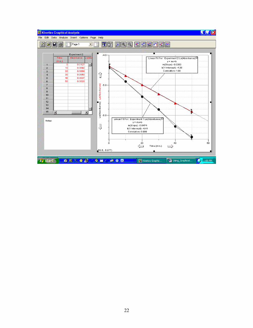
Kinetics This exercise is designed to familiarize you with plotting two or more data sets on one graph and how to have the program take the natural log (Ln) of all data sets. A study is made of the reaction: 2N2O5(g) → 4NO2(g) + O2(g) and the following data obtained. A plot of Ln[N2O5] versus Time will give a straight line if the reaction is first order in N2O5.. A graph of Ln[N2O5] (y-axis) versus time (x-axis) will be plotted from the following two data sets. You can also plot Ln(Absorbance) versus time from Absorbance and time data using the same technique. Experiment Number 1 Experiment Number 2

Time, Min. [N2O5], M Time, Min. [N2O5], M 0.0 0.0124 0.0 0.0127

10.0 0.0076 10.0 0.0092 20.0 0.0046 20.0 0.0068 30.0 0.0030 30.0 0.0050 40.0 0.0017 40.0 0.0037 50.0 0.0012 50.0 0.0028

7

Open the graphical analysis program and double click in the x data set box and type in Time for the label and min. for the units. By clicking on the Options tab you can vary the color and style of your data points and set the significant figures displayed. Then click OK.

\

8

By double clicking on the y data set box you can enter Absorbance for the y-axis label and adjust the options similar to the x data. Remember there are no units for absorbance. Then click OK.

9

Now click on Data and click on New calculated column on the drop down menu.

Type in Ln(Absorbance) in the name box and in the short name box. Click on the Functions arrow and select ln[]. Click on the Variables arrow and select Absorbance. Be sure the y-axis box is checked. Then click OK.

10

Click on Data in the bar menu and click on New Data Set.

11

A new data set will appear in the data table. You can add 4 data sets for the kinetics experiment. Click on the Data Set (and then Data Set 2 ) and type in Experiment 1 and Experiment 2 respectively.

12

Click on Data and then on New Calculated column in the drop down menu.

13

Type in Ln(Absorbance) in the Name and Short Name spaces. Click on the Functions arrow and select ln(). Click on the Variables (Columns) arrow and select Absorbance. Then click OK.

14

Now add the time and absorbance data to the appropriate columns. The Absorbance versus Time data is automatically plotted. The new Ln(Absorbance) column is automatically calculated.

15

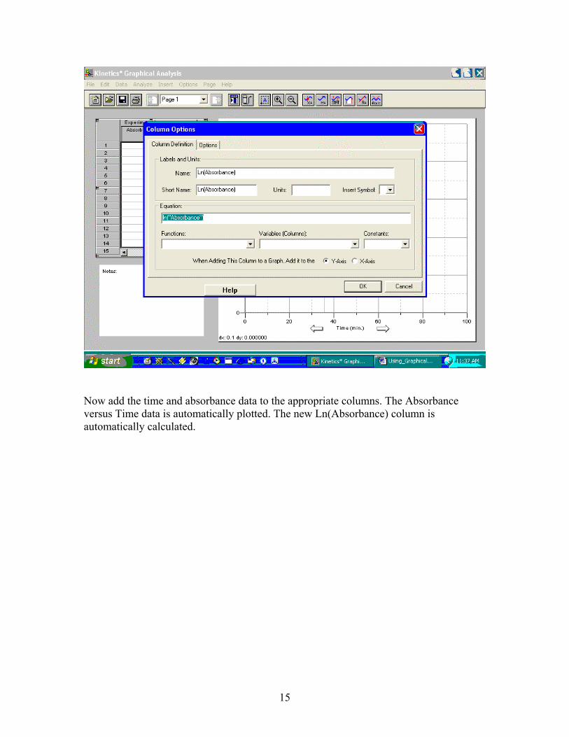
Click on the Absorbance label in the graph, remove the check mark from the Absorbance box and add a check mark to the Ln(Absorbance box. Then click OK. The graph of Ln(Absorbance) is then displayed.

16

17

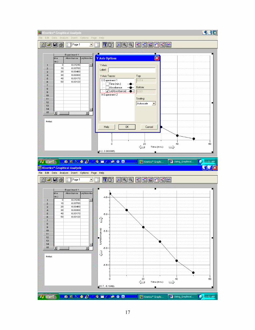
Now enter the data set for experiment number 2. Click the Ln(Absorbance) label on the graph, click on data set 2 and check Ln(Absorbance in both data sets 1 and 2. Then click OK.

18

Click on the R= icon on the next to last icon in the bar menu for the linear regression or best fit through the data points. Then click OK.

19

.

20

By putting the cursor in each linear fit box on the graph and holding down the left click you can move them to convenient locations.

21

22