Embed Size (px)
Citation preview
x = 1 let x = 1 in ...
x(1).
!x(1) x.set(1)
Introduction to Haskell
Ralf Lämmel
Programming Paradigms and Formal Semantics
© Ralf Lämmel, 2009-2011 unless noted otherwise 2
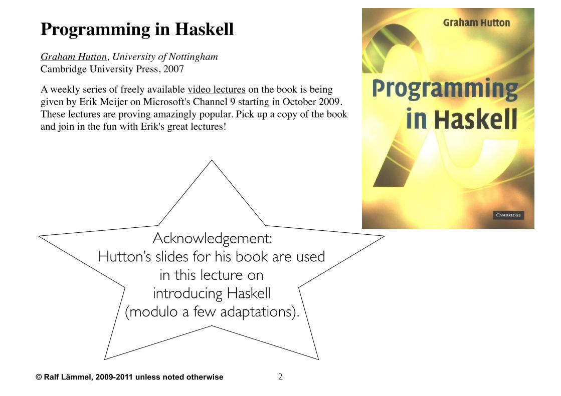
Programming in HaskellGraham Hutton, University of NottinghamCambridge University Press, 2007
A weekly series of freely available video lectures on the book is being given by Erik Meijer on Microsoft's Channel 9 starting in October 2009. These lectures are proving amazingly popular. Pick up a copy of the book and join in the fun with Erik's great lectures!
Acknowledgement: Hutton’s slides for his book are used
in this lecture on introducing Haskell
(modulo a few adaptations).
© Ralf Lämmel, 2009-2011 unless noted otherwise
This slide deck is derived from G. Hutton’s deck for his book ”Programming in Haskell”,
3
What is a Functional Language?
© Ralf Lämmel, 2009-2011 unless noted otherwise
This slide deck is derived from G. Hutton’s deck for his book ”Programming in Haskell”,
4
What is a Functional Language?
๏Functional programming is style of programming in which the basic method of computation is the application of functions to arguments;
๏A functional language is one that supports and encourages the functional style.
Opinions differ, and it is difficult to give a precise definition, but generally speaking:
© Ralf Lämmel, 2009-2011 unless noted otherwise
\This slide deck is derived from G. Hutton’s deck for his book ”Programming in Haskell”,
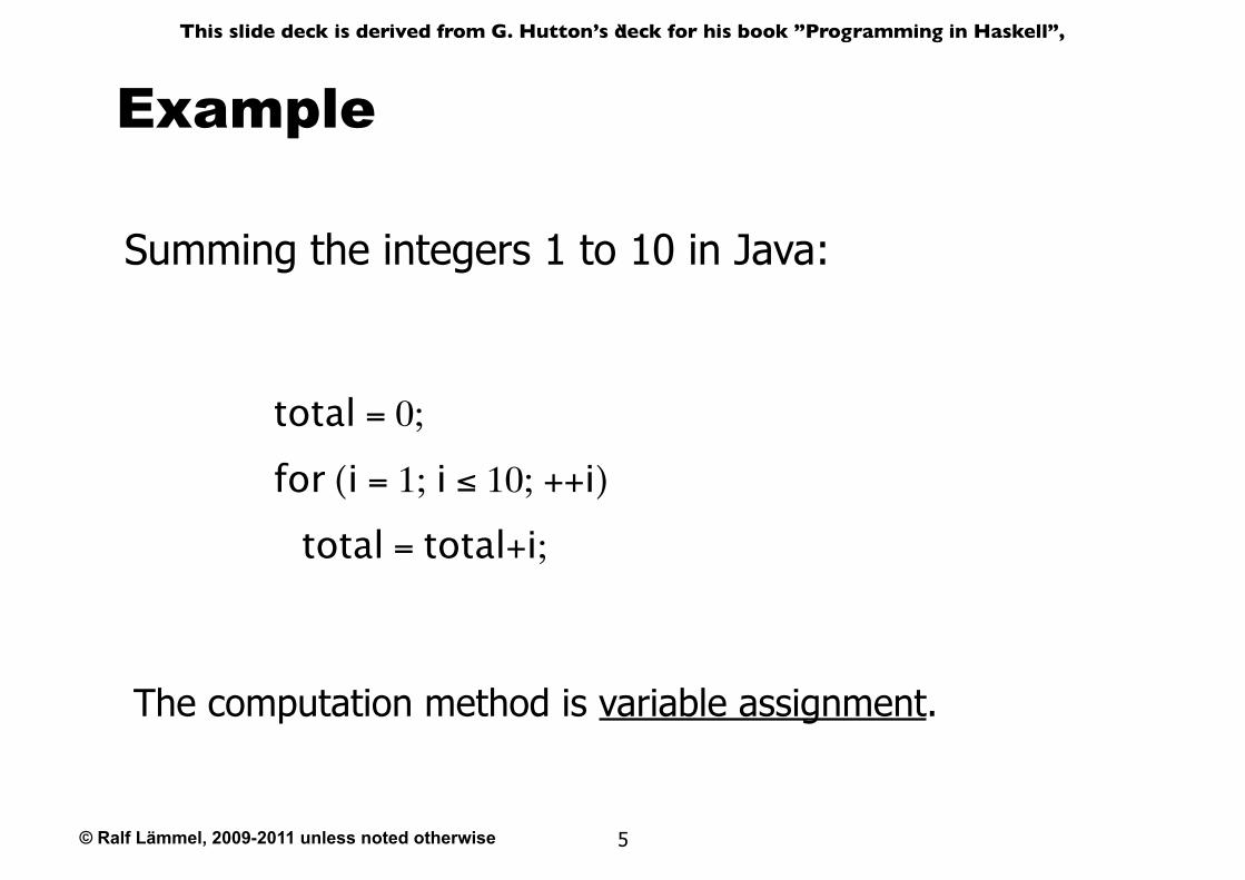
Example
Summing the integers 1 to 10 in Java:
total = 0;
for (i = 1; i ≤ 10; ++i) total = total+i;
The computation method is variable assignment.
5
© Ralf Lämmel, 2009-2011 unless noted otherwise
\This slide deck is derived from G. Hutton’s deck for his book ”Programming in Haskell”,
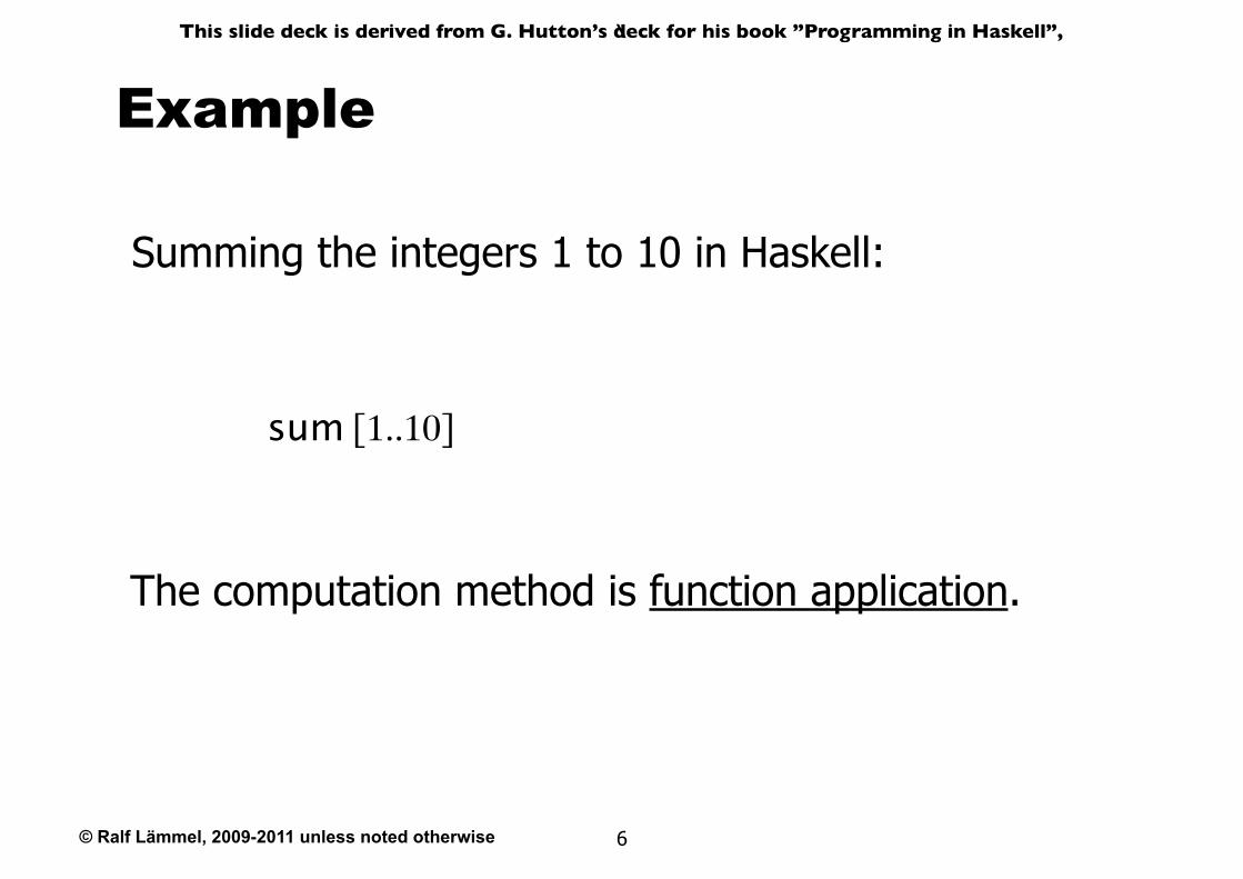
Example
Summing the integers 1 to 10 in Haskell:
sum [1..10]
The computation method is function application.
6
© Ralf Lämmel, 2009-2011 unless noted otherwise
\This slide deck is derived from G. Hutton’s deck for his book ”Programming in Haskell”,
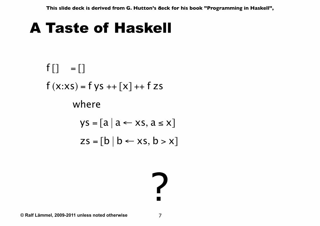
A Taste of Haskell
f [] = []
f (x:xs) = f ys ++ [x] ++ f zs
where
ys = [a | a ← xs, a ≤ x]
zs = [b | b ← xs, b > x]
?7
© Ralf Lämmel, 2009-2011 unless noted otherwise
This slide deck is derived from G. Hutton’s deck for his book ”Programming in Haskell”,
8
Historical Background
© Ralf Lämmel, 2009-2011 unless noted otherwise
\This slide deck is derived from G. Hutton’s deck for his book ”Programming in Haskell”,
Historical Background
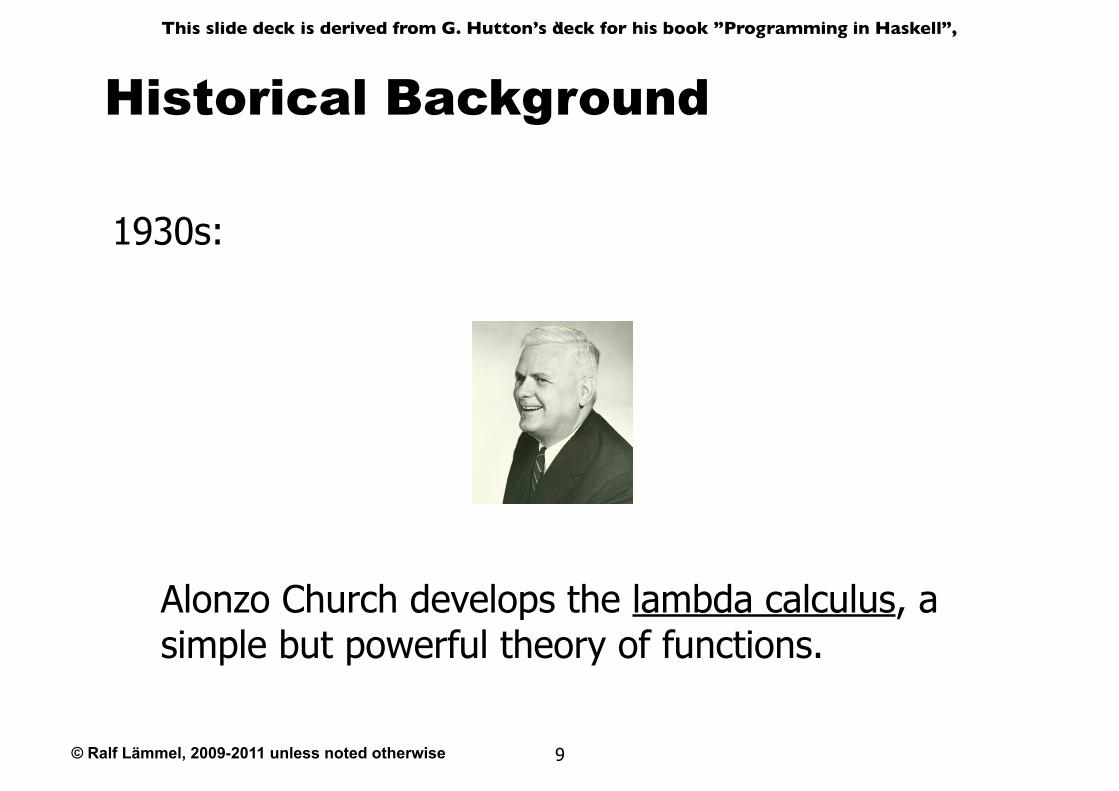
1930s:
Alonzo Church develops the lambda calculus, a simple but powerful theory of functions.
9
© Ralf Lämmel, 2009-2011 unless noted otherwise
\This slide deck is derived from G. Hutton’s deck for his book ”Programming in Haskell”,
Historical Background
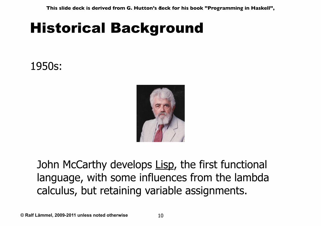
1950s:
John McCarthy develops Lisp, the first functional language, with some influences from the lambda calculus, but retaining variable assignments.
10
© Ralf Lämmel, 2009-2011 unless noted otherwise
\This slide deck is derived from G. Hutton’s deck for his book ”Programming in Haskell”,
Historical Background
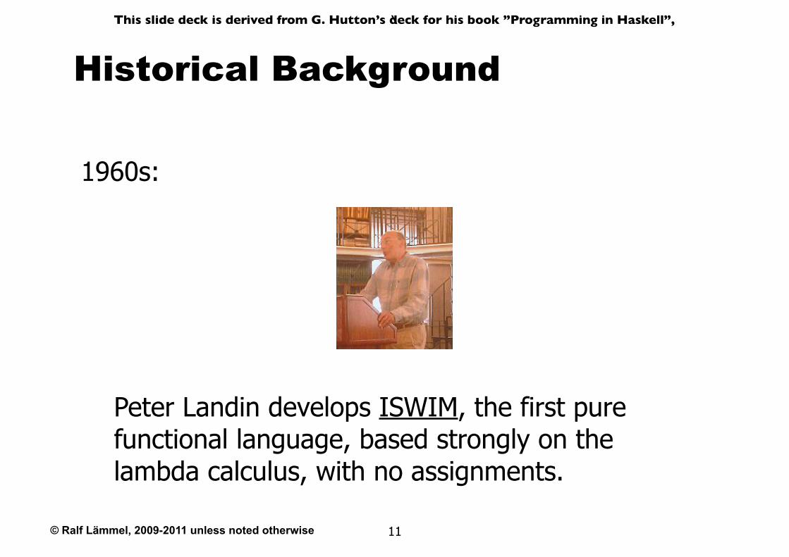
1960s:
Peter Landin develops ISWIM, the first pure functional language, based strongly on the lambda calculus, with no assignments.
11
© Ralf Lämmel, 2009-2011 unless noted otherwise
\This slide deck is derived from G. Hutton’s deck for his book ”Programming in Haskell”,
Historical Background
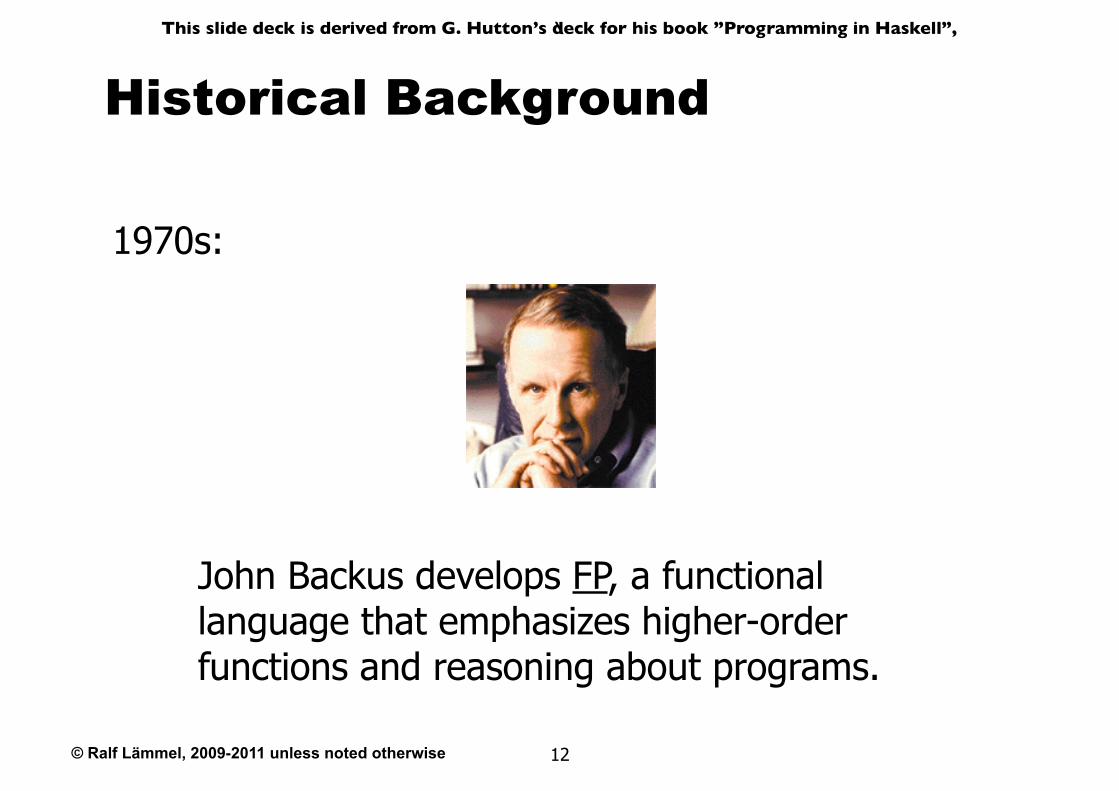
1970s:
John Backus develops FP, a functional language that emphasizes higher-order functions and reasoning about programs.
12
© Ralf Lämmel, 2009-2011 unless noted otherwise
\This slide deck is derived from G. Hutton’s deck for his book ”Programming in Haskell”,
Historical Background
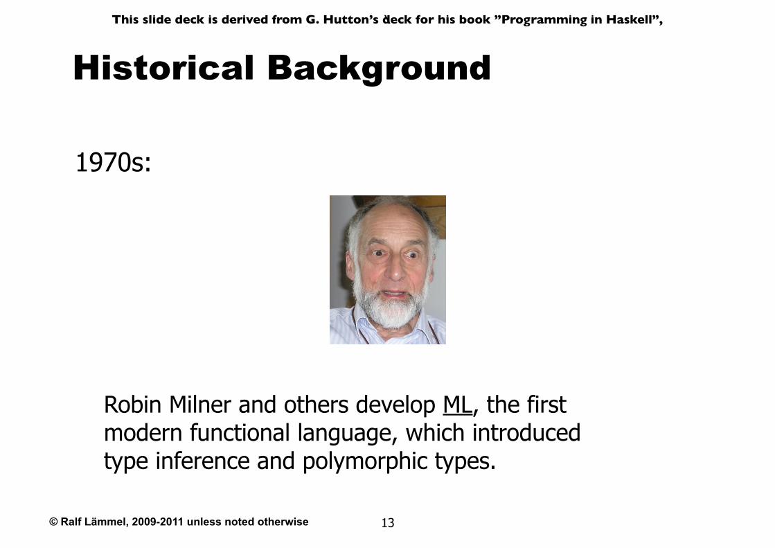
1970s:
Robin Milner and others develop ML, the first modern functional language, which introduced type inference and polymorphic types.
13
© Ralf Lämmel, 2009-2011 unless noted otherwise
\This slide deck is derived from G. Hutton’s deck for his book ”Programming in Haskell”,
Historical Background
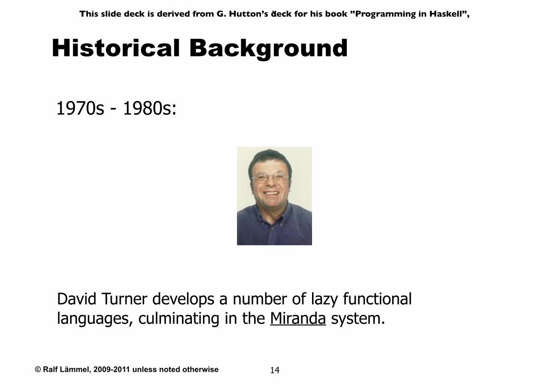
1970s - 1980s:
David Turner develops a number of lazy functional languages, culminating in the Miranda system.
14
© Ralf Lämmel, 2009-2011 unless noted otherwise
\This slide deck is derived from G. Hutton’s deck for his book ”Programming in Haskell”,
Historical Background
1987:
An international committee of researchers initiates the development of Haskell, a standard lazy functional language.
15
© Ralf Lämmel, 2009-2011 unless noted otherwise
\This slide deck is derived from G. Hutton’s deck for his book ”Programming in Haskell”,
Historical Background
2003:
The committee publishes the Haskell 98 report, defining a stable version of the language.
16
© Ralf Lämmel, 2009-2011 unless noted otherwise
This slide deck is derived from G. Hutton’s deck for his book ”Programming in Haskell”,
17
First Steps in Haskell
© Ralf Lämmel, 2009-2011 unless noted otherwise
This slide deck is derived from G. Hutton’s deck for his book ”Programming in Haskell”,
18
Haskell systems
★http://www.haskell.org/
★Major option: GHC
http://haskell.org/ghc/download.html
© Ralf Lämmel, 2009-2011 unless noted otherwise
This slide deck is derived from G. Hutton’s deck for his book ”Programming in Haskell”,
19
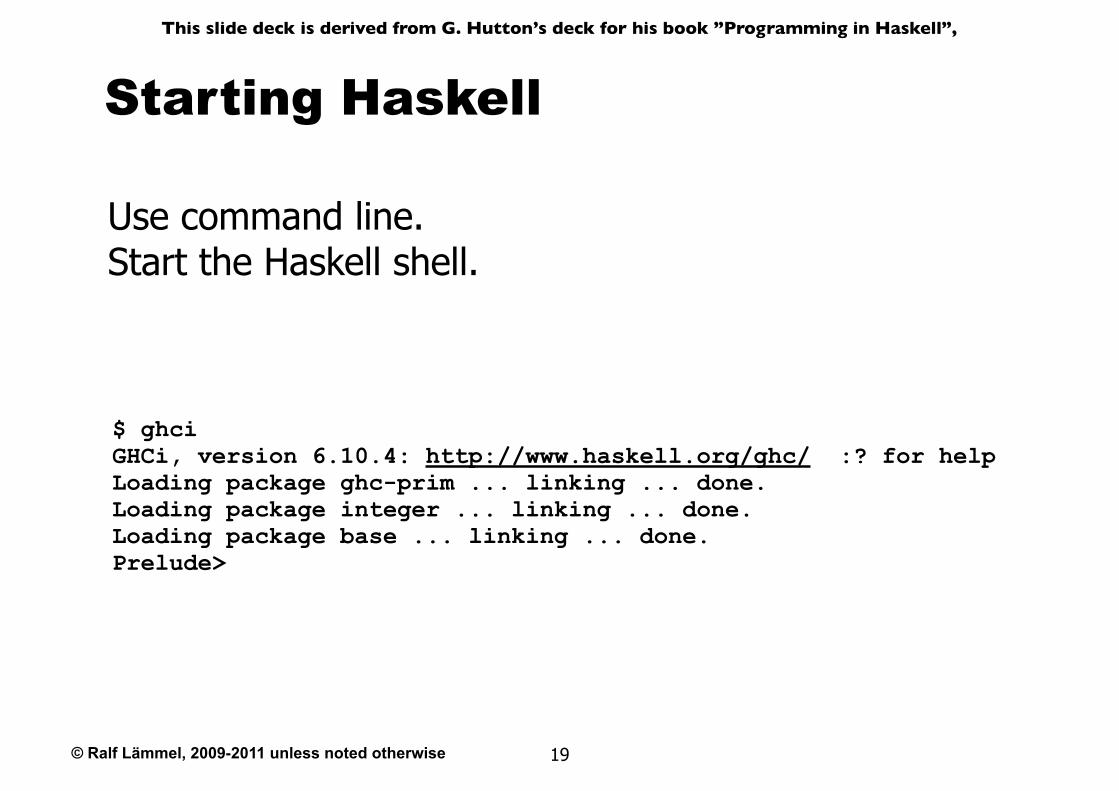
Starting Haskell
Use command line.Start the Haskell shell.
$ ghciGHCi, version 6.10.4: http://www.haskell.org/ghc/ :? for helpLoading package ghc-prim ... linking ... done.Loading package integer ... linking ... done.Loading package base ... linking ... done.Prelude>
© Ralf Lämmel, 2009-2011 unless noted otherwise
This slide deck is derived from G. Hutton’s deck for his book ”Programming in Haskell”,
20
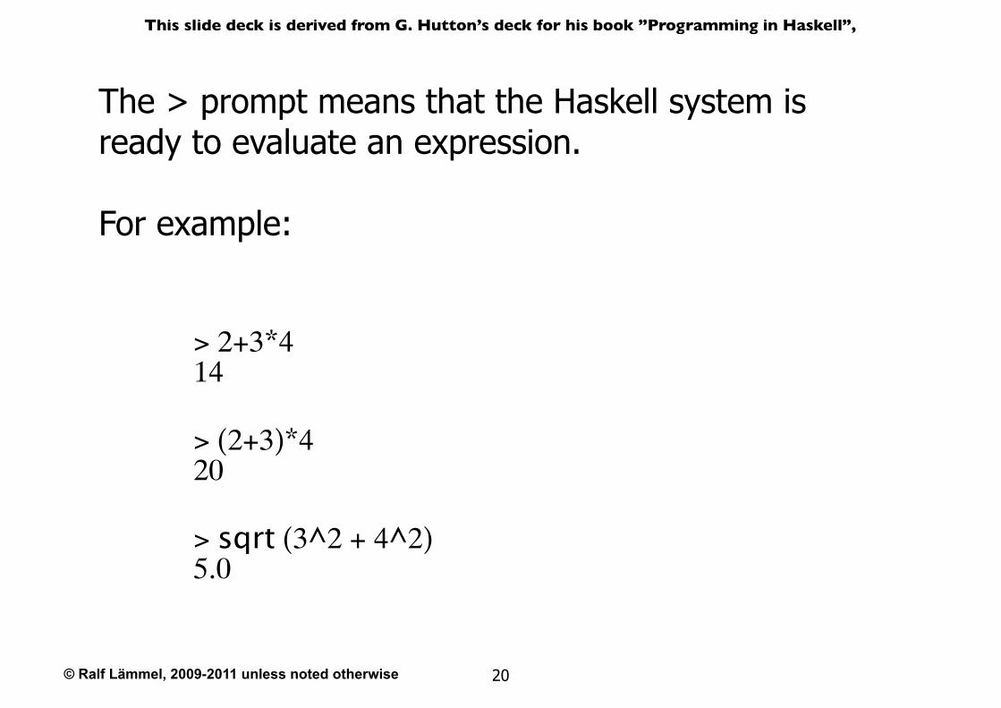
The > prompt means that the Haskell system is ready to evaluate an expression.
For example:
> 2+3*414
> (2+3)*420
> sqrt (3^2 + 4^2)5.0
© Ralf Lämmel, 2009-2011 unless noted otherwise
This slide deck is derived from G. Hutton’s deck for his book ”Programming in Haskell”,
21
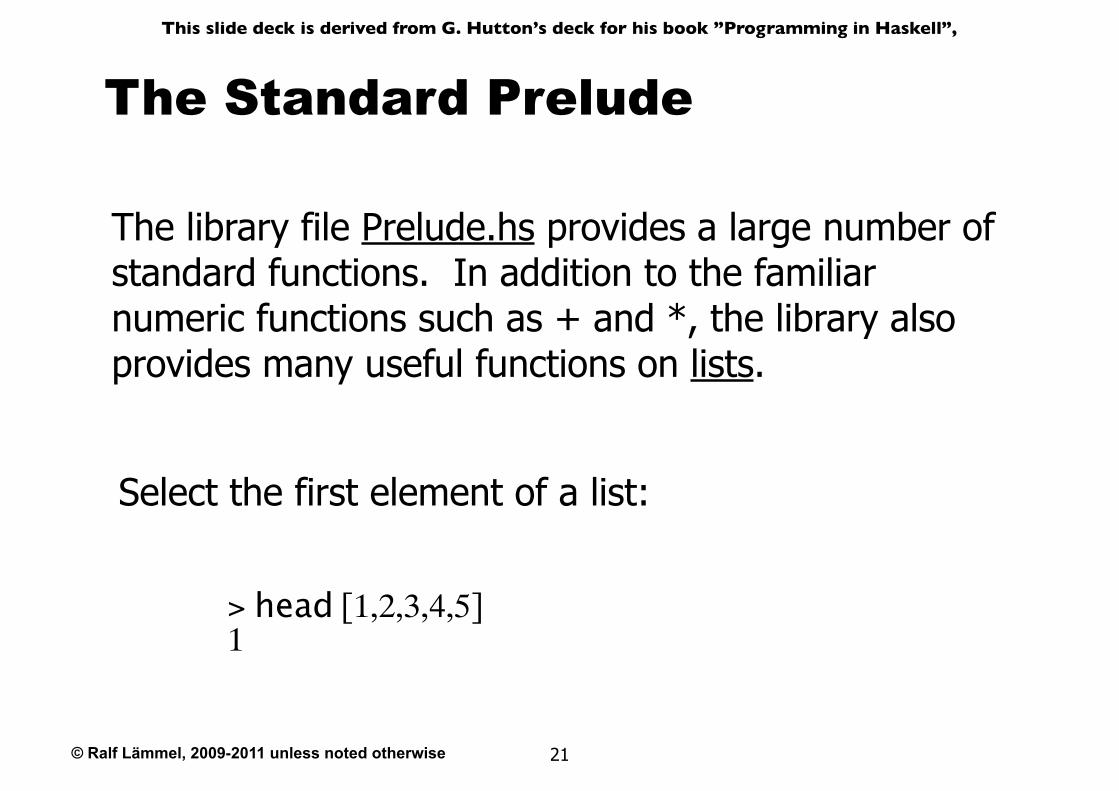
The Standard Prelude
The library file Prelude.hs provides a large number of standard functions. In addition to the familiar numeric functions such as + and *, the library also provides many useful functions on lists.
Select the first element of a list:
> head [1,2,3,4,5]1
© Ralf Lämmel, 2009-2011 unless noted otherwise
This slide deck is derived from G. Hutton’s deck for his book ”Programming in Haskell”,
22
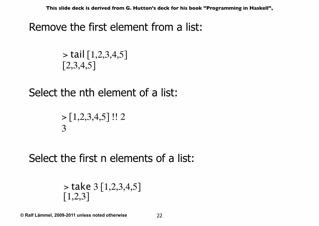
Remove the first element from a list:
> tail [1,2,3,4,5][2,3,4,5]
Select the nth element of a list:
> [1,2,3,4,5] !! 23
Select the first n elements of a list:
> take 3 [1,2,3,4,5][1,2,3]
© Ralf Lämmel, 2009-2011 unless noted otherwise
This slide deck is derived from G. Hutton’s deck for his book ”Programming in Haskell”,
23
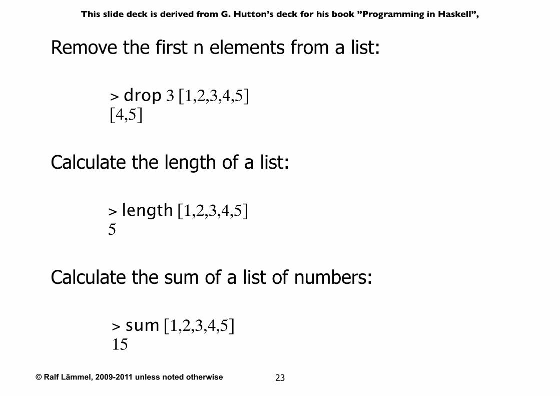
Remove the first n elements from a list:
> drop 3 [1,2,3,4,5][4,5]
Calculate the length of a list:
> length [1,2,3,4,5]5
Calculate the sum of a list of numbers:
> sum [1,2,3,4,5]15
© Ralf Lämmel, 2009-2011 unless noted otherwise
This slide deck is derived from G. Hutton’s deck for his book ”Programming in Haskell”,
24
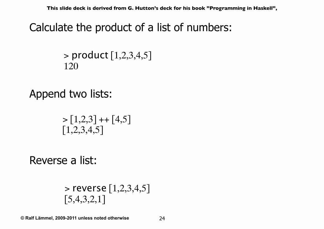
Calculate the product of a list of numbers:
> product [1,2,3,4,5]120
Append two lists:
> [1,2,3] ++ [4,5][1,2,3,4,5]
Reverse a list:
> reverse [1,2,3,4,5][5,4,3,2,1]
© Ralf Lämmel, 2009-2011 unless noted otherwise
This slide deck is derived from G. Hutton’s deck for his book ”Programming in Haskell”,
25
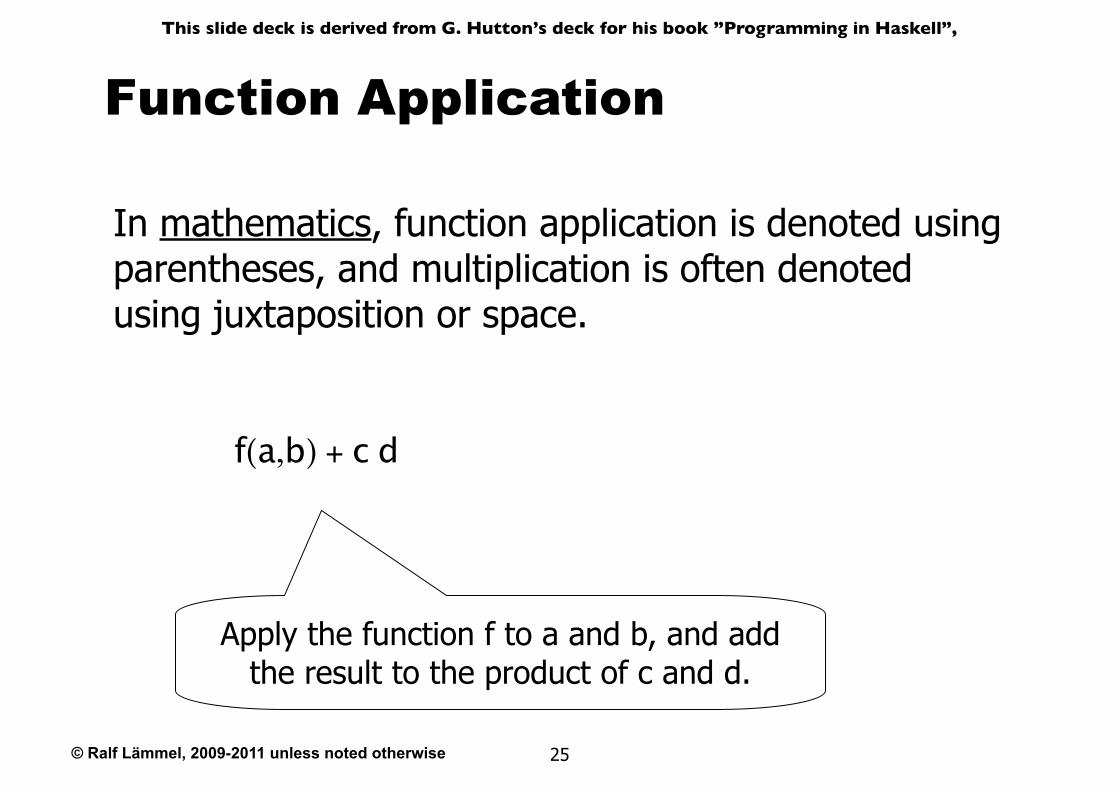
Function Application
In mathematics, function application is denoted using parentheses, and multiplication is often denoted using juxtaposition or space.
f(a,b) + c d
Apply the function f to a and b, and add the result to the product of c and d.
© Ralf Lämmel, 2009-2011 unless noted otherwise
This slide deck is derived from G. Hutton’s deck for his book ”Programming in Haskell”,
26
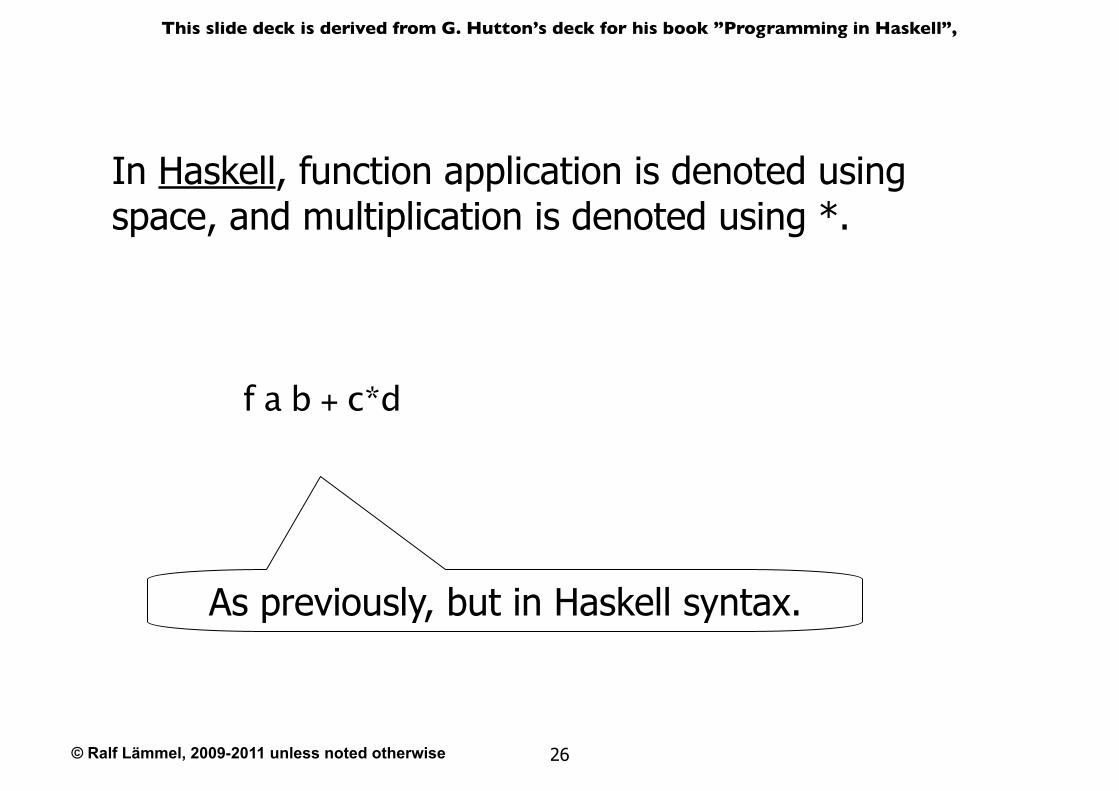
In Haskell, function application is denoted using space, and multiplication is denoted using *.
f a b + c*d
As previously, but in Haskell syntax.
© Ralf Lämmel, 2009-2011 unless noted otherwise
This slide deck is derived from G. Hutton’s deck for his book ”Programming in Haskell”,
27
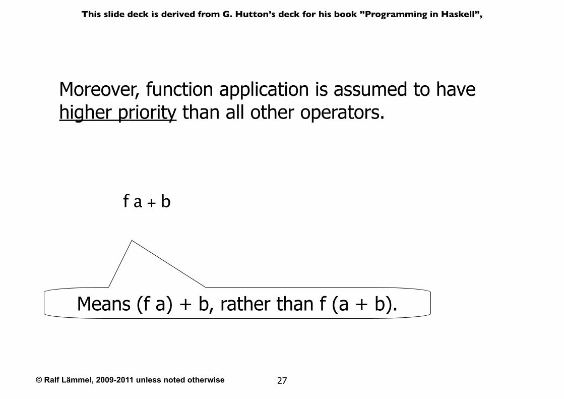
Moreover, function application is assumed to have higher priority than all other operators.
f a + b
Means (f a) + b, rather than f (a + b).
© Ralf Lämmel, 2009-2011 unless noted otherwise
This slide deck is derived from G. Hutton’s deck for his book ”Programming in Haskell”,
28
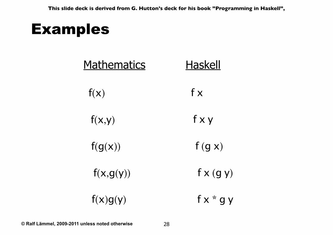
Examples
Mathematics Haskell
f(x)
f(x,y)
f(g(x))
f(x,g(y))
f(x)g(y)
f x
f x y
f (g x)
f x (g y)
f x * g y
© Ralf Lämmel, 2009-2011 unless noted otherwise
This slide deck is derived from G. Hutton’s deck for his book ”Programming in Haskell”,
29
Haskell Scripts
★As well as the functions in the standard prelude, you can also define your own functions;
★New functions are defined within a script, a text file comprising a sequence of definitions;
★By convention, Haskell scripts usually have a .hs suffix on their filename. This is not mandatory, but is useful for identification purposes.
© Ralf Lämmel, 2009-2011 unless noted otherwise
This slide deck is derived from G. Hutton’s deck for his book ”Programming in Haskell”,
30
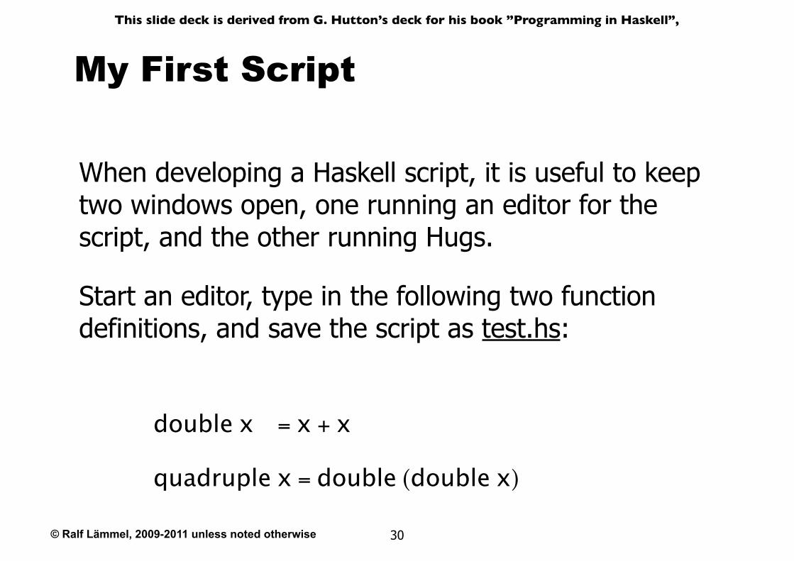
My First Script
double x = x + x
quadruple x = double (double x)
When developing a Haskell script, it is useful to keep two windows open, one running an editor for the script, and the other running Hugs.
Start an editor, type in the following two function definitions, and save the script as test.hs:
© Ralf Lämmel, 2009-2011 unless noted otherwise
This slide deck is derived from G. Hutton’s deck for his book ”Programming in Haskell”,
31
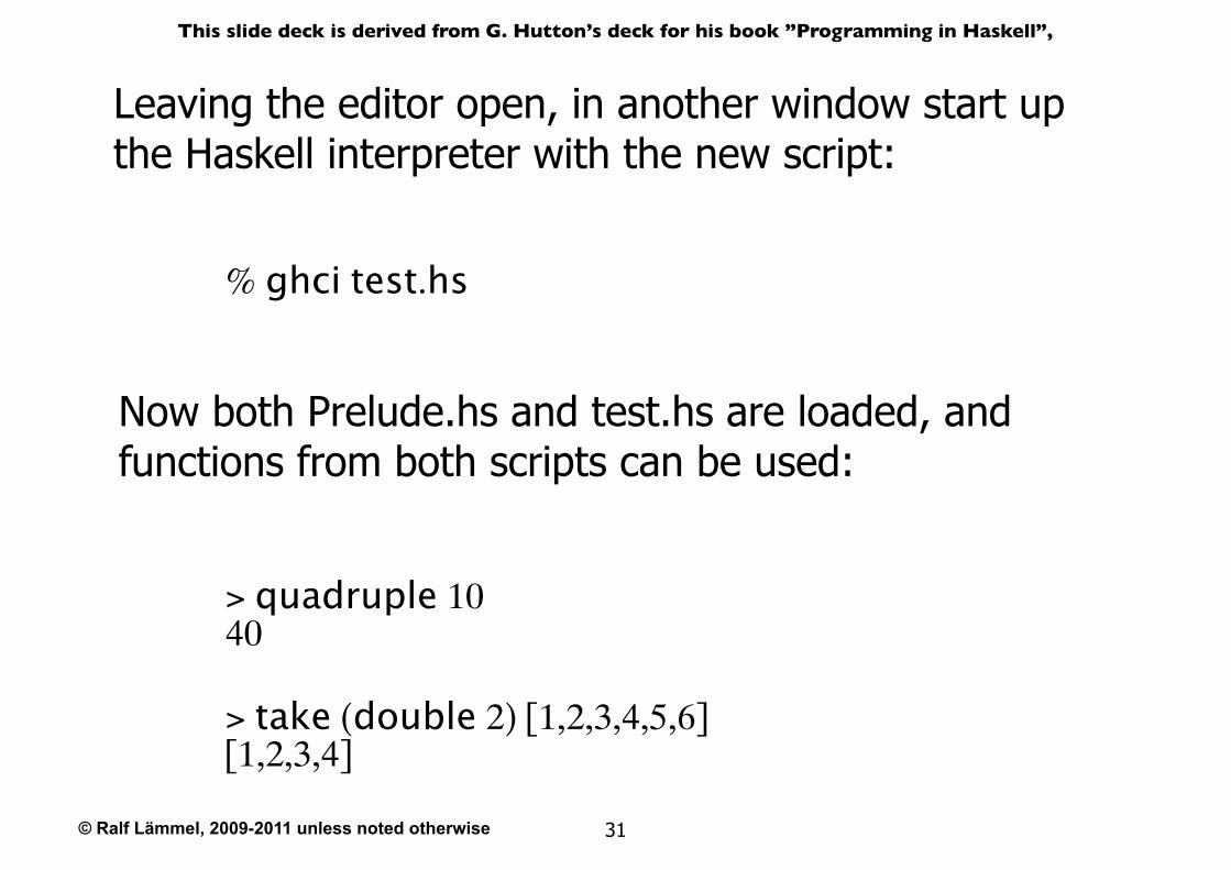
% ghci test.hs
Leaving the editor open, in another window start up the Haskell interpreter with the new script:
> quadruple 1040
> take (double 2) [1,2,3,4,5,6][1,2,3,4]
Now both Prelude.hs and test.hs are loaded, and functions from both scripts can be used:
© Ralf Lämmel, 2009-2011 unless noted otherwise
This slide deck is derived from G. Hutton’s deck for his book ”Programming in Haskell”,
32
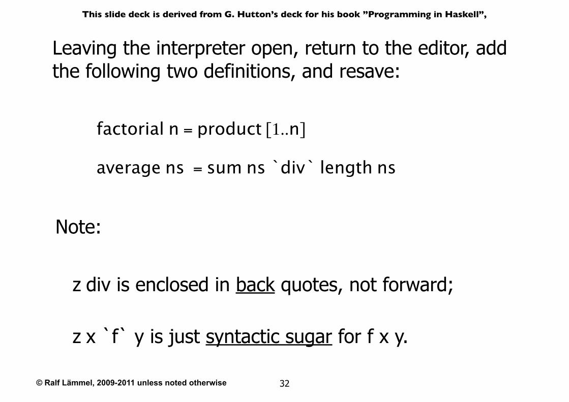
factorial n = product [1..n]
average ns = sum ns `div` length ns
Leaving the interpreter open, return to the editor, add the following two definitions, and resave:
z div is enclosed in back quotes, not forward;
z x `f` y is just syntactic sugar for f x y.
Note:
© Ralf Lämmel, 2009-2011 unless noted otherwise
This slide deck is derived from G. Hutton’s deck for his book ”Programming in Haskell”,
33
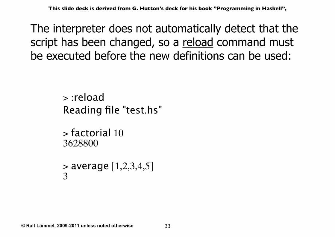
> :reloadReading file "test.hs"
> factorial 103628800
> average [1,2,3,4,5]3
The interpreter does not automatically detect that the script has been changed, so a reload command must be executed before the new definitions can be used:
© Ralf Lämmel, 2009-2011 unless noted otherwise
This slide deck is derived from G. Hutton’s deck for his book ”Programming in Haskell”,
34
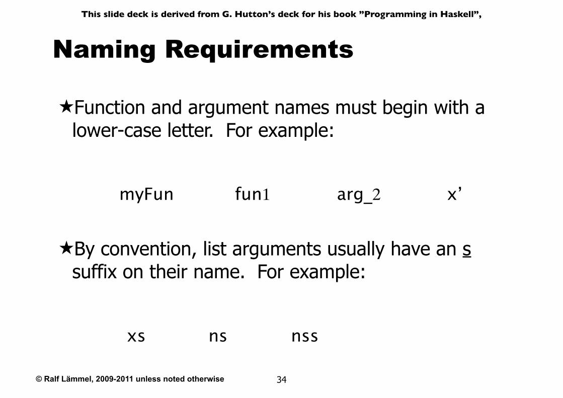
Naming Requirements
★Function and argument names must begin with a lower-case letter. For example:
myFun fun1 arg_2 x’
★By convention, list arguments usually have an s suffix on their name. For example:
xs ns nss
© Ralf Lämmel, 2009-2011 unless noted otherwise
This slide deck is derived from G. Hutton’s deck for his book ”Programming in Haskell”,
35
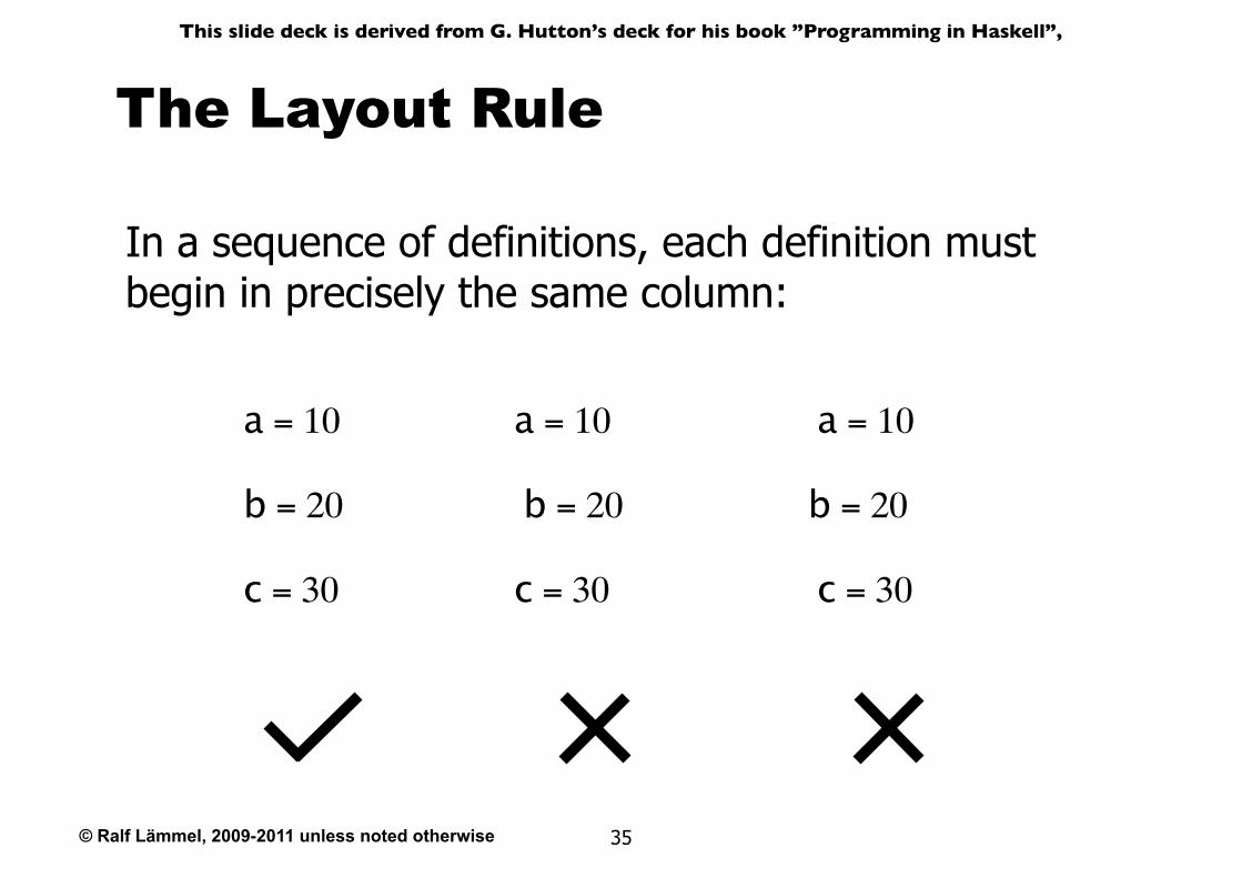
The Layout Rule
In a sequence of definitions, each definition must begin in precisely the same column:
a = 10
b = 20
c = 30
a = 10
b = 20
c = 30
a = 10
b = 20
c = 30
© Ralf Lämmel, 2009-2011 unless noted otherwise
This slide deck is derived from G. Hutton’s deck for his book ”Programming in Haskell”,
36
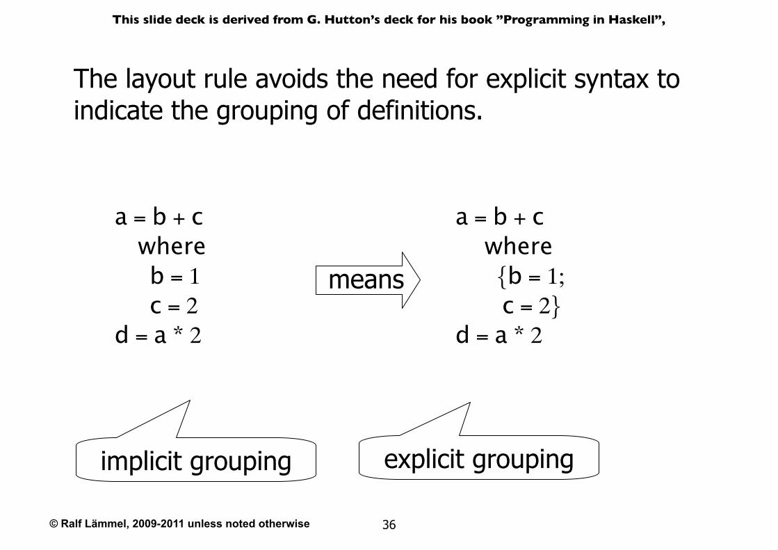
means
The layout rule avoids the need for explicit syntax to indicate the grouping of definitions.
a = b + c where b = 1 c = 2d = a * 2
a = b + c where {b = 1; c = 2}d = a * 2
implicit grouping explicit grouping
© Ralf Lämmel, 2009-2011 unless noted otherwise
This slide deck is derived from G. Hutton’s deck for his book ”Programming in Haskell”,
37
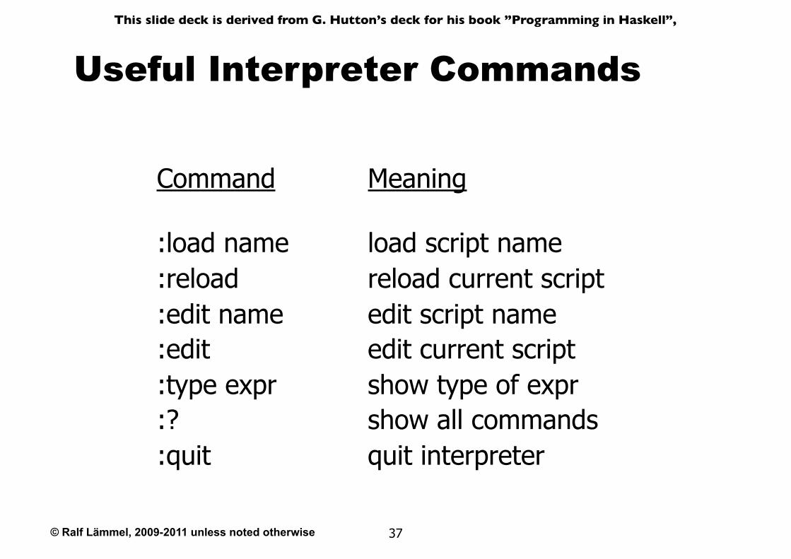
Useful Interpreter Commands
Command Meaning
:load name load script name:reload reload current script:edit name edit script name:edit edit current script:type expr show type of expr:? show all commands:quit quit interpreter
© Ralf Lämmel, 2009-2011 unless noted otherwise
This slide deck is derived from G. Hutton’s deck for his book ”Programming in Haskell”,
38
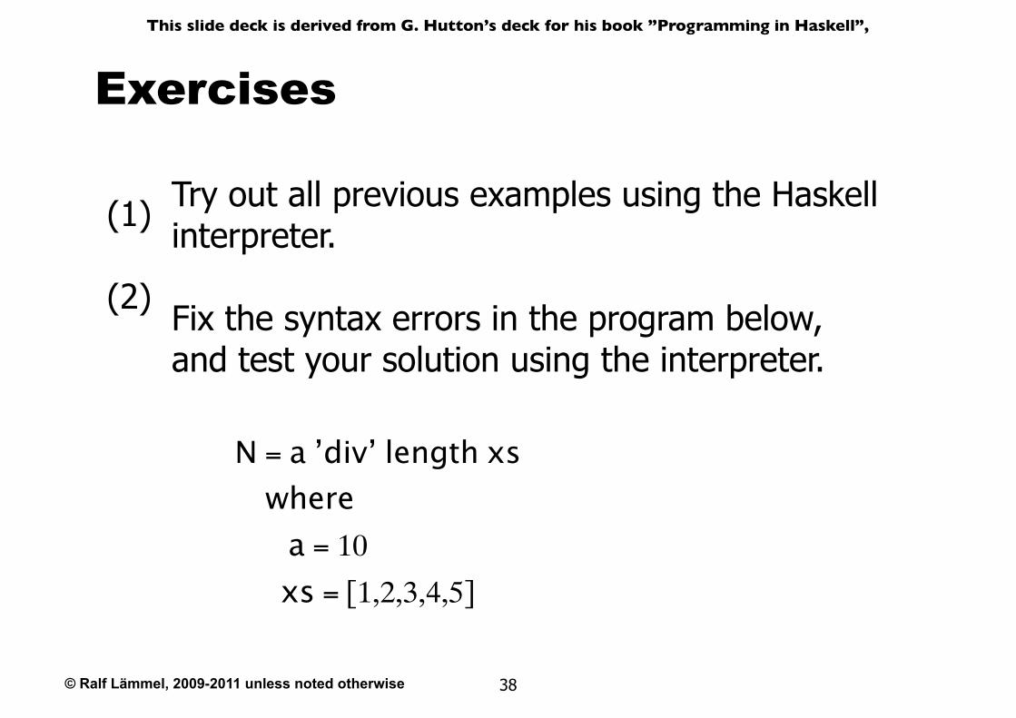
Exercises
N = a ’div’ length xs where a = 10
xs = [1,2,3,4,5]
Try out all previous examples using the Haskell interpreter.
Fix the syntax errors in the program below, and test your solution using the interpreter.
(1)
(2)
© Ralf Lämmel, 2009-2011 unless noted otherwise
This slide deck is derived from G. Hutton’s deck for his book ”Programming in Haskell”,
39
Show how the library function last that selects the last element of a list can be defined using the functions introduced in this lecture.
(3)
Similarly, show how the library function init that removes the last element from a list can be defined in two different ways.
(5)
Can you think of another possible definition?(4)
© Ralf Lämmel, 2009-2011 unless noted otherwise
This slide deck is derived from G. Hutton’s deck for his book ”Programming in Haskell”,
40
Common Types
© Ralf Lämmel, 2009-2011 unless noted otherwise
This slide deck is derived from G. Hutton’s deck for his book ”Programming in Haskell”,
41
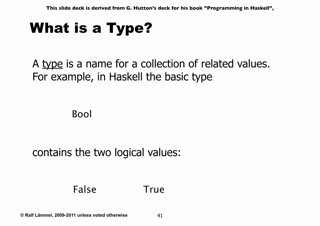
What is a Type?
A type is a name for a collection of related values. For example, in Haskell the basic type
TrueFalse
Bool
contains the two logical values:
© Ralf Lämmel, 2009-2011 unless noted otherwise
This slide deck is derived from G. Hutton’s deck for his book ”Programming in Haskell”,
42
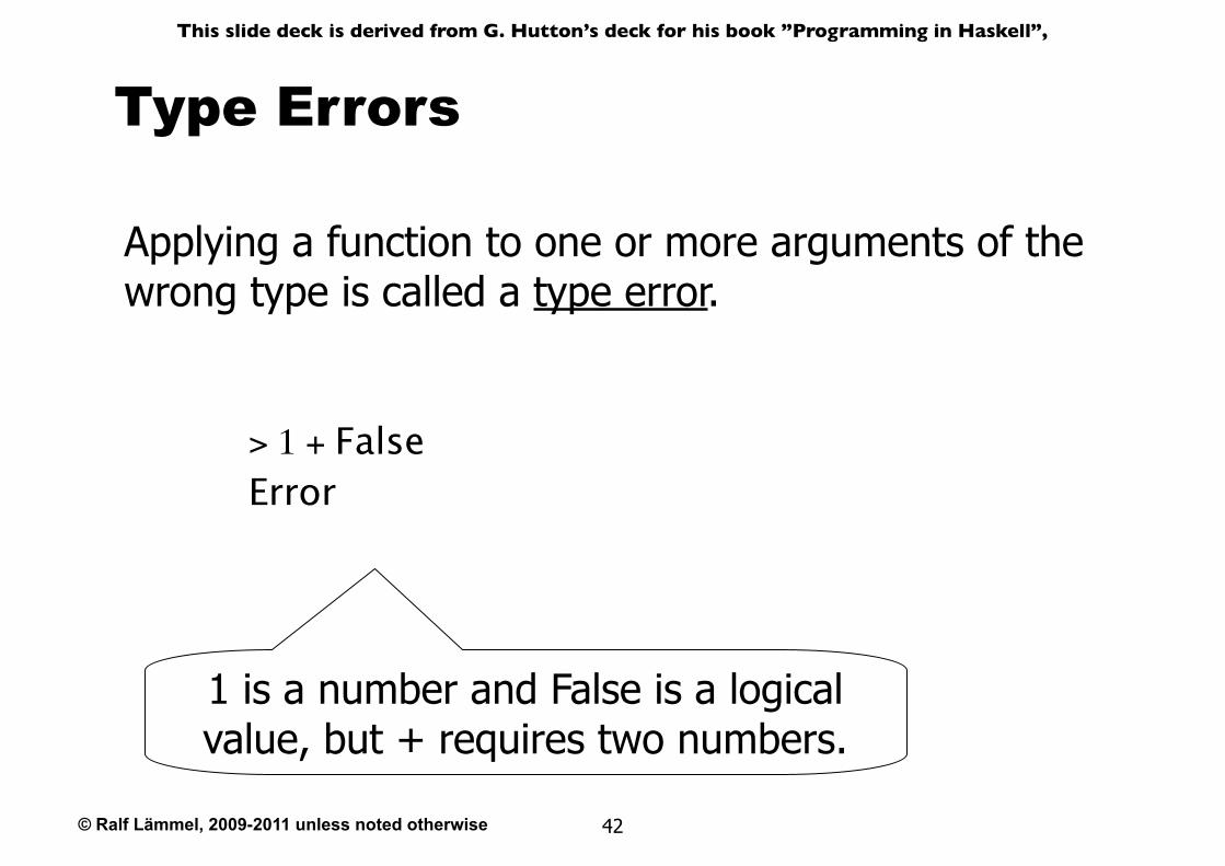
Type Errors
Applying a function to one or more arguments of the wrong type is called a type error.
> 1 + FalseError
1 is a number and False is a logical value, but + requires two numbers.
© Ralf Lämmel, 2009-2011 unless noted otherwise
This slide deck is derived from G. Hutton’s deck for his book ”Programming in Haskell”,
43
Types in Haskell
★If evaluating an expression e would produce a value of type t, then e has type t, written
e :: t
★Every well formed expression has a type, which can be automatically calculated at compile time using a process called type inference.
© Ralf Lämmel, 2009-2011 unless noted otherwise
This slide deck is derived from G. Hutton’s deck for his book ”Programming in Haskell”,
44
★All type errors are found at compile time, which makes programs safer and faster by removing the need for type checks at run time.
★In the Haskell interpreter, the :type command calculates the type of an expression, without evaluating it:
> not FalseTrue
> :type not Falsenot False :: Bool
© Ralf Lämmel, 2009-2011 unless noted otherwise
This slide deck is derived from G. Hutton’s deck for his book ”Programming in Haskell”,
45
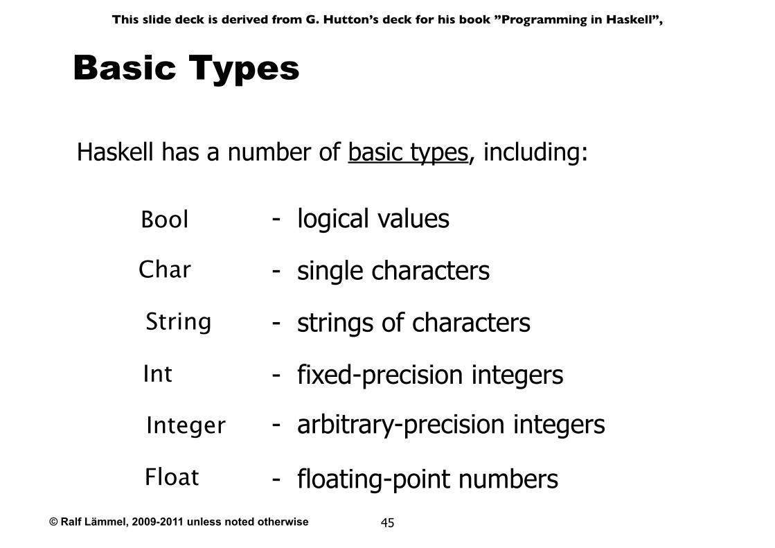
Basic Types
Haskell has a number of basic types, including:
Bool - logical values
Char - single characters
Integer - arbitrary-precision integers
Float - floating-point numbers
String - strings of characters
Int - fixed-precision integers
© Ralf Lämmel, 2009-2011 unless noted otherwise
This slide deck is derived from G. Hutton’s deck for his book ”Programming in Haskell”,
46
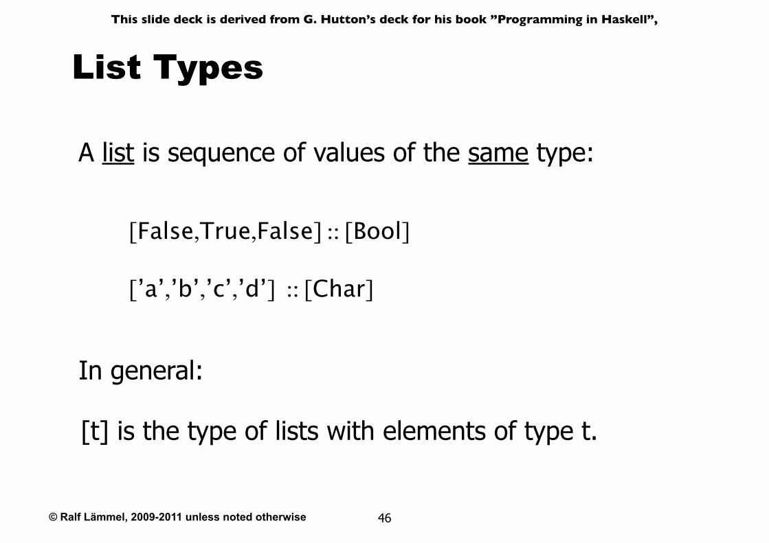
List Types
[False,True,False] :: [Bool]
[’a’,’b’,’c’,’d’] :: [Char]
In general:
A list is sequence of values of the same type:
[t] is the type of lists with elements of type t.
© Ralf Lämmel, 2009-2011 unless noted otherwise
This slide deck is derived from G. Hutton’s deck for his book ”Programming in Haskell”,
47
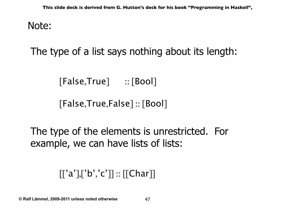
The type of a list says nothing about its length:
[False,True] :: [Bool]
[False,True,False] :: [Bool]
[[’a’],[’b’,’c’]] :: [[Char]]
Note:
The type of the elements is unrestricted. For example, we can have lists of lists:
© Ralf Lämmel, 2009-2011 unless noted otherwise
This slide deck is derived from G. Hutton’s deck for his book ”Programming in Haskell”,
48
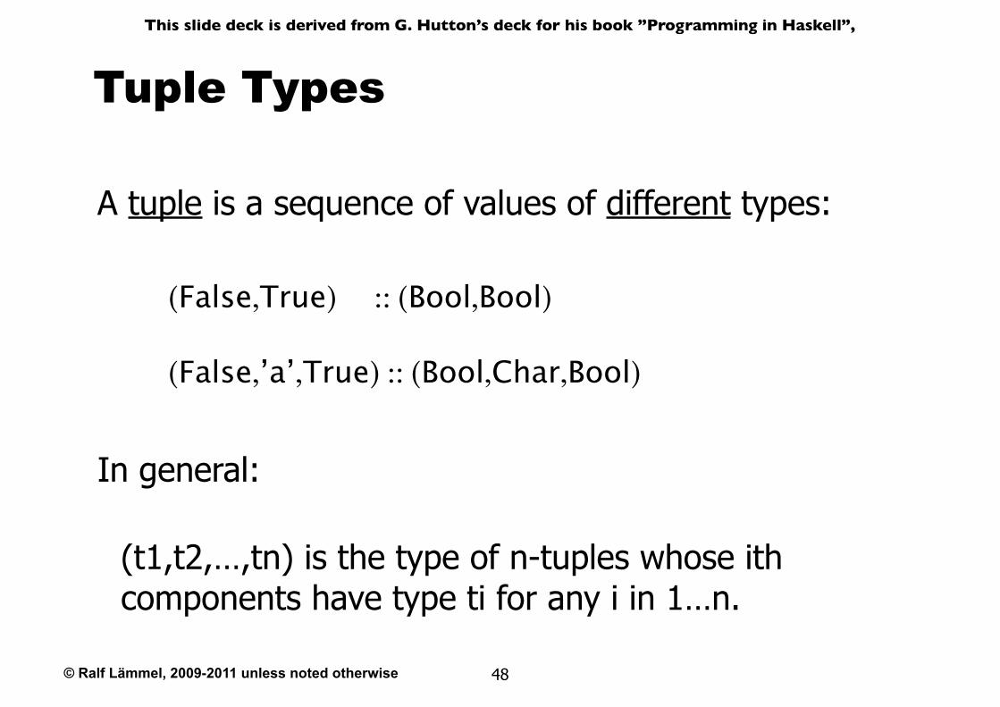
Tuple Types
A tuple is a sequence of values of different types:
(False,True) :: (Bool,Bool)
(False,’a’,True) :: (Bool,Char,Bool)
In general:
(t1,t2,…,tn) is the type of n-tuples whose ith components have type ti for any i in 1…n.
© Ralf Lämmel, 2009-2011 unless noted otherwise
This slide deck is derived from G. Hutton’s deck for his book ”Programming in Haskell”,
49
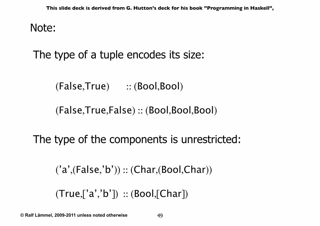
The type of a tuple encodes its size:
(False,True) :: (Bool,Bool)
(False,True,False) :: (Bool,Bool,Bool)
(’a’,(False,’b’)) :: (Char,(Bool,Char))
(True,[’a’,’b’]) :: (Bool,[Char])
Note:
The type of the components is unrestricted:
© Ralf Lämmel, 2009-2011 unless noted otherwise
This slide deck is derived from G. Hutton’s deck for his book ”Programming in Haskell”,
50
Hints and Tips
★When defining a new function in Haskell, it is useful to begin by writing down its type;
★Within a script, it is good practice to state the type of every new function defined;
© Ralf Lämmel, 2009-2011 unless noted otherwise
This slide deck is derived from G. Hutton’s deck for his book ”Programming in Haskell”,
51
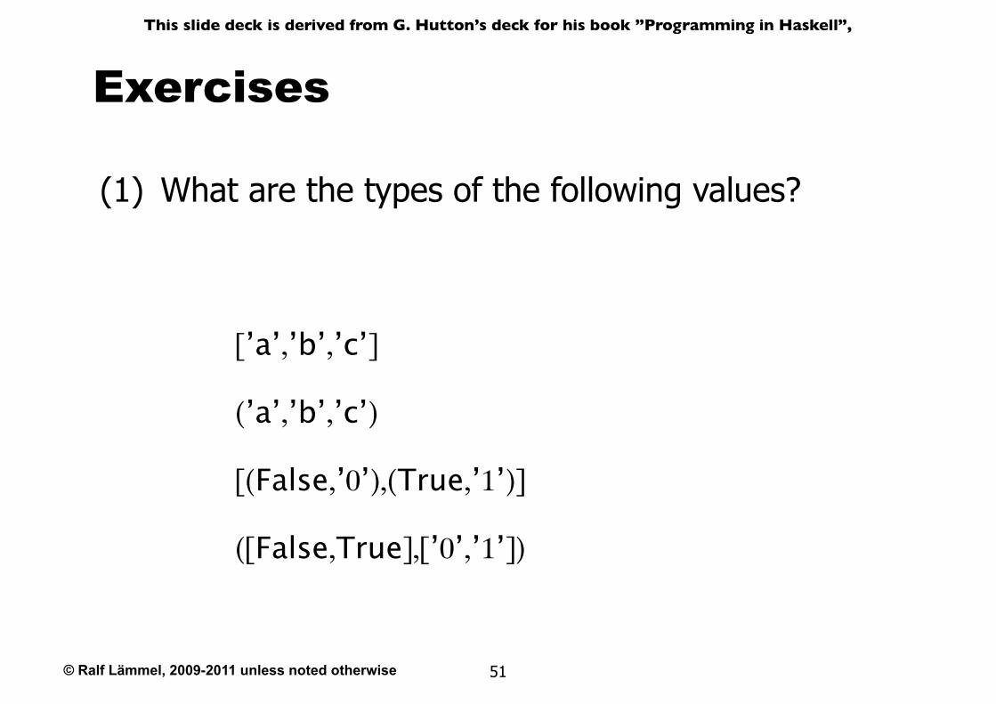
Exercises
[’a’,’b’,’c’]
(’a’,’b’,’c’)
[(False,’0’),(True,’1’)]
([False,True],[’0’,’1’])
What are the types of the following values?(1)
© Ralf Lämmel, 2009-2011 unless noted otherwise
This slide deck is derived from G. Hutton’s deck for his book ”Programming in Haskell”,
52
Functions types
© Ralf Lämmel, 2009-2011 unless noted otherwise
This slide deck is derived from G. Hutton’s deck for his book ”Programming in Haskell”,
53
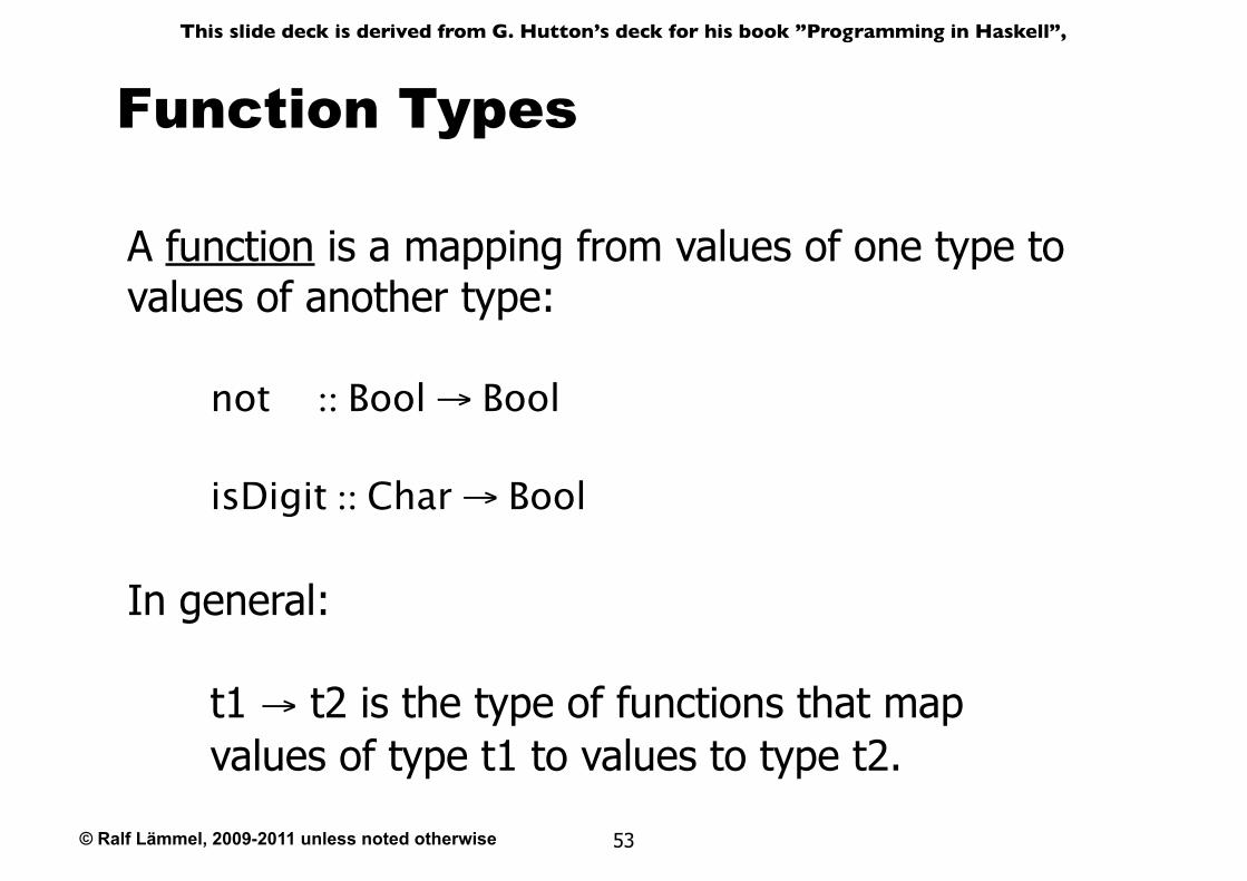
Function Types
not :: Bool → Bool
isDigit :: Char → Bool
In general:
A function is a mapping from values of one type to values of another type:
t1 → t2 is the type of functions that map values of type t1 to values to type t2.
© Ralf Lämmel, 2009-2011 unless noted otherwise
This slide deck is derived from G. Hutton’s deck for his book ”Programming in Haskell”,
54
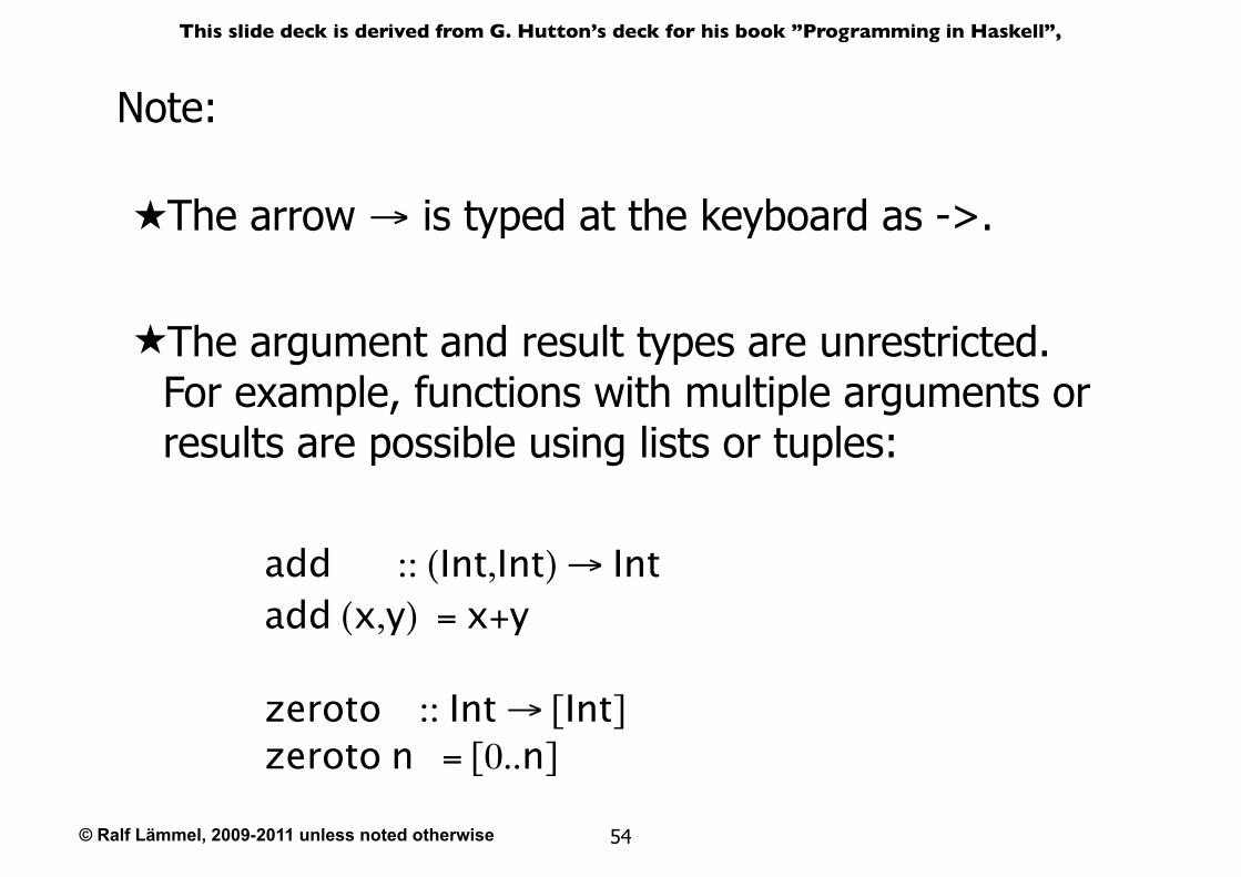
★The arrow → is typed at the keyboard as ->.
★The argument and result types are unrestricted. For example, functions with multiple arguments or results are possible using lists or tuples:
Note:
add :: (Int,Int) → Intadd (x,y) = x+y
zeroto :: Int → [Int]zeroto n = [0..n]
© Ralf Lämmel, 2009-2011 unless noted otherwise
This slide deck is derived from G. Hutton’s deck for his book ”Programming in Haskell”,
55
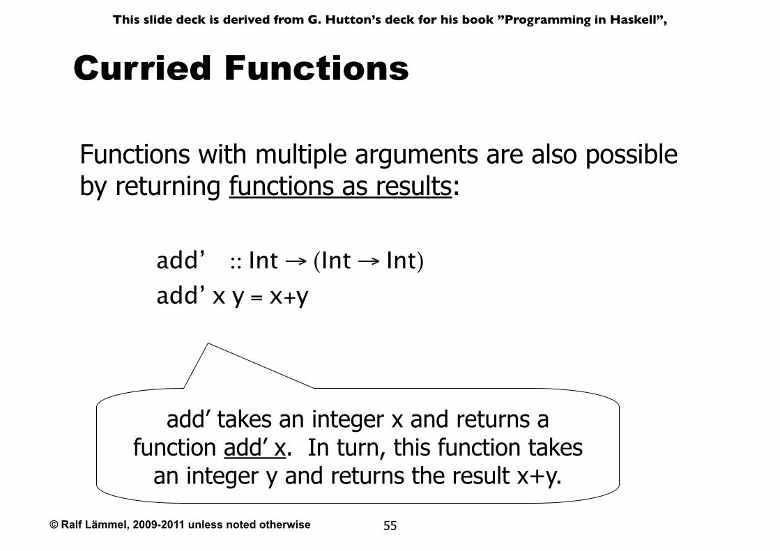
Functions with multiple arguments are also possible by returning functions as results:
add’ :: Int → (Int → Int)add’ x y = x+y
add’ takes an integer x and returns a function add’ x. In turn, this function takes
an integer y and returns the result x+y.
Curried Functions
© Ralf Lämmel, 2009-2011 unless noted otherwise
This slide deck is derived from G. Hutton’s deck for his book ”Programming in Haskell”,
56
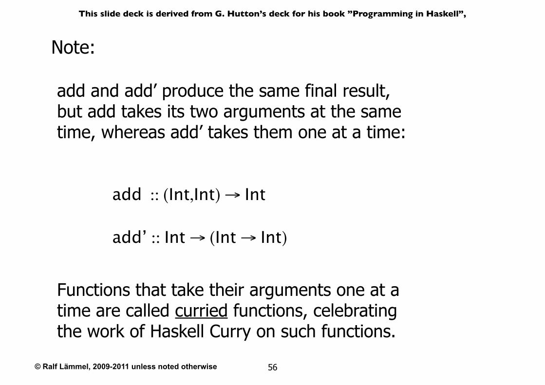
add and add’ produce the same final result, but add takes its two arguments at the same time, whereas add’ takes them one at a time:
Note:
Functions that take their arguments one at a time are called curried functions, celebrating the work of Haskell Curry on such functions.
add :: (Int,Int) → Int
add’ :: Int → (Int → Int)
© Ralf Lämmel, 2009-2011 unless noted otherwise
This slide deck is derived from G. Hutton’s deck for his book ”Programming in Haskell”,
57
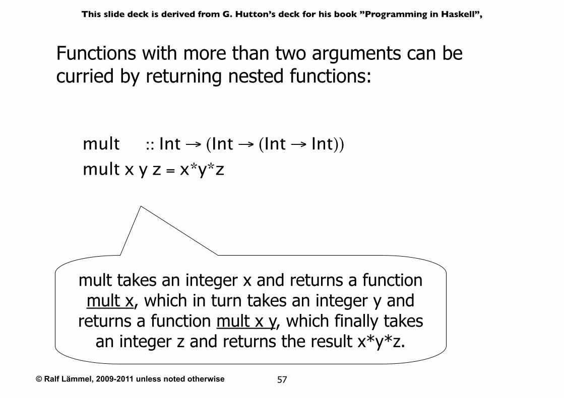
Functions with more than two arguments can be curried by returning nested functions:
mult :: Int → (Int → (Int → Int))mult x y z = x*y*z
mult takes an integer x and returns a function mult x, which in turn takes an integer y and
returns a function mult x y, which finally takes an integer z and returns the result x*y*z.
© Ralf Lämmel, 2009-2011 unless noted otherwise
This slide deck is derived from G. Hutton’s deck for his book ”Programming in Haskell”,
58
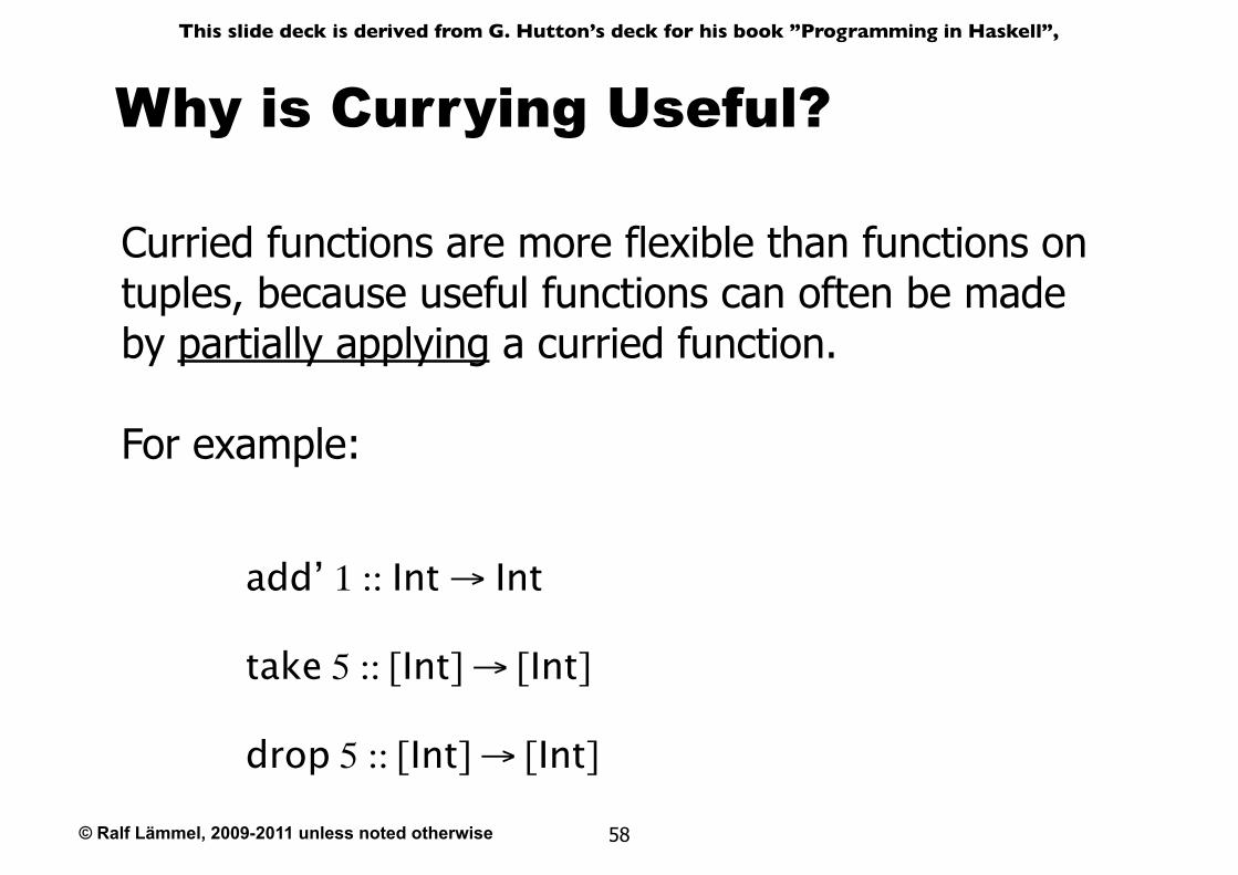
Why is Currying Useful?
Curried functions are more flexible than functions on tuples, because useful functions can often be made by partially applying a curried function.
For example:
add’ 1 :: Int → Int
take 5 :: [Int] → [Int]
drop 5 :: [Int] → [Int]
© Ralf Lämmel, 2009-2011 unless noted otherwise
This slide deck is derived from G. Hutton’s deck for his book ”Programming in Haskell”,
59
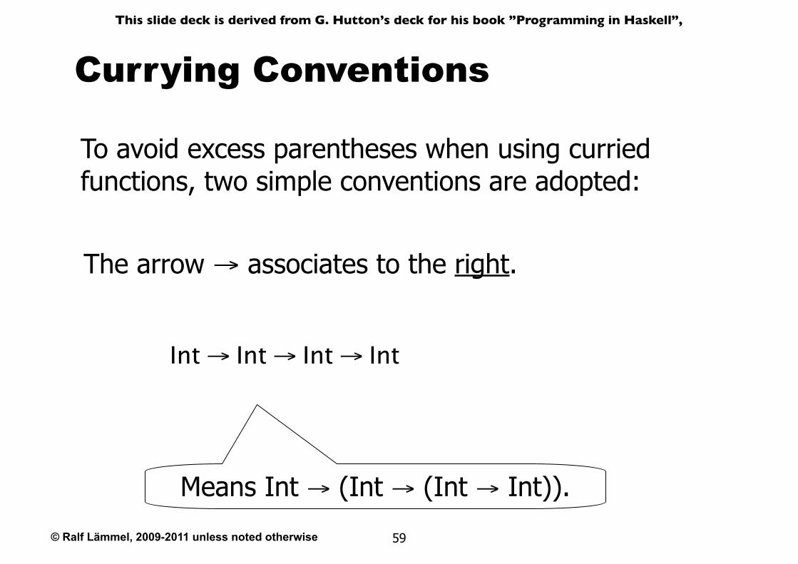
Currying Conventions
The arrow → associates to the right.
Int → Int → Int → Int
To avoid excess parentheses when using curried functions, two simple conventions are adopted:
Means Int → (Int → (Int → Int)).
© Ralf Lämmel, 2009-2011 unless noted otherwise
This slide deck is derived from G. Hutton’s deck for his book ”Programming in Haskell”,
60
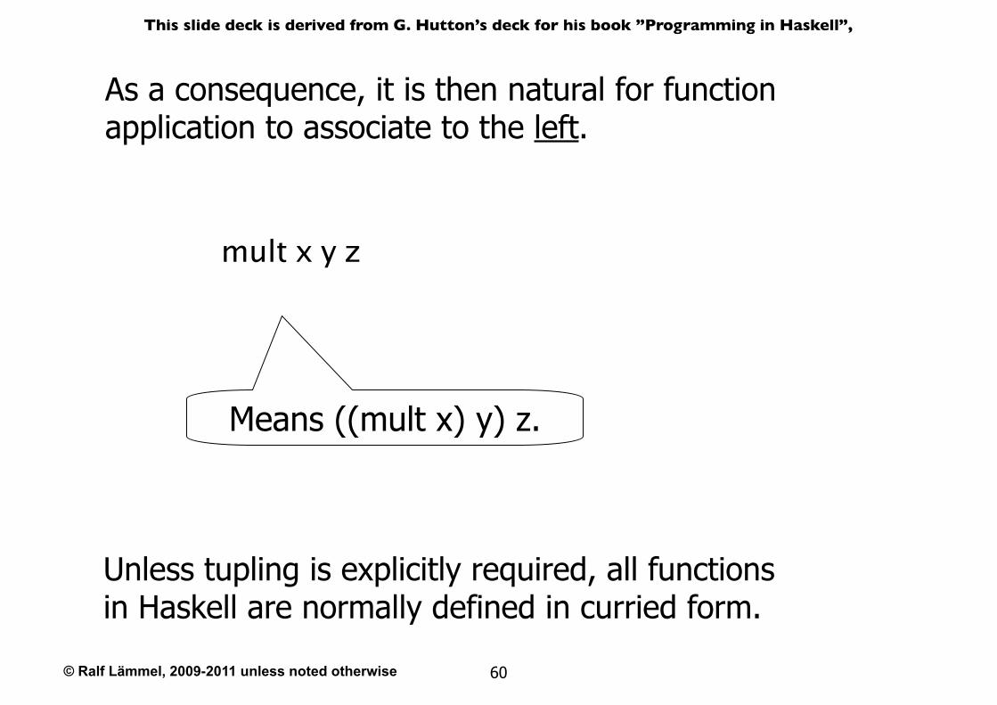
As a consequence, it is then natural for function application to associate to the left.
mult x y z
Means ((mult x) y) z.
Unless tupling is explicitly required, all functions in Haskell are normally defined in curried form.
© Ralf Lämmel, 2009-2011 unless noted otherwise
This slide deck is derived from G. Hutton’s deck for his book ”Programming in Haskell”,
61
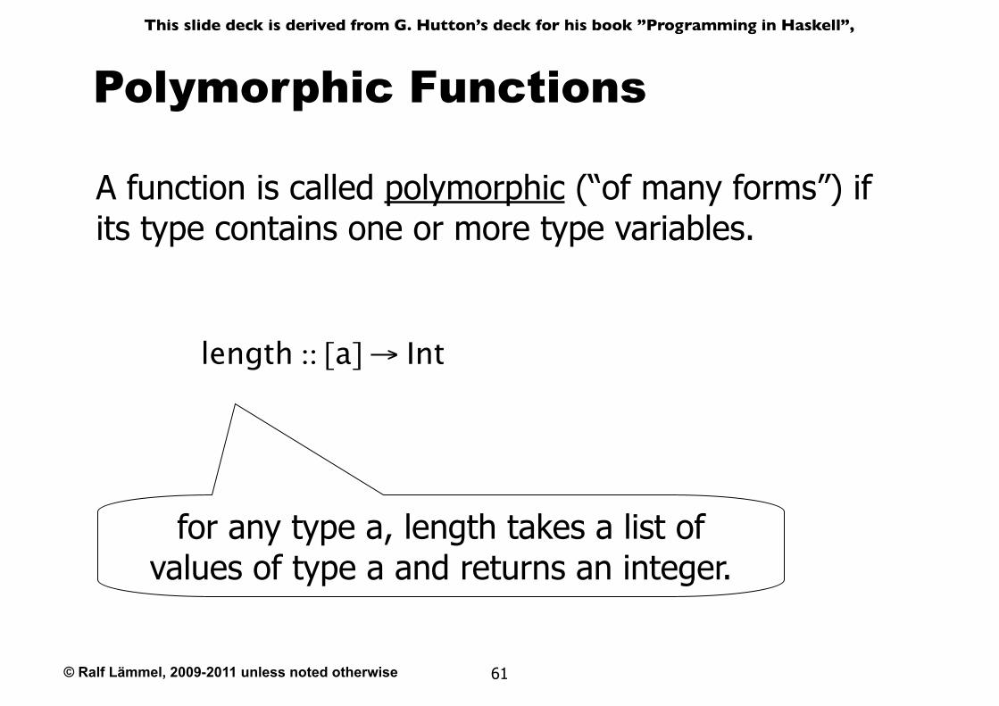
Polymorphic Functions
A function is called polymorphic (“of many forms”) if its type contains one or more type variables.
length :: [a] → Int
for any type a, length takes a list of values of type a and returns an integer.
© Ralf Lämmel, 2009-2011 unless noted otherwise
This slide deck is derived from G. Hutton’s deck for his book ”Programming in Haskell”,
62
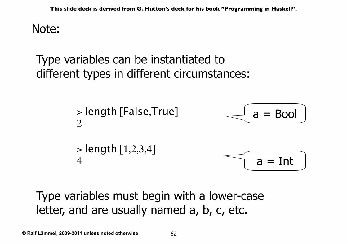
Type variables can be instantiated to different types in different circumstances:
Note:
Type variables must begin with a lower-case letter, and are usually named a, b, c, etc.
> length [False,True]2
> length [1,2,3,4]4
a = Bool
a = Int
© Ralf Lämmel, 2009-2011 unless noted otherwise
This slide deck is derived from G. Hutton’s deck for his book ”Programming in Haskell”,
63
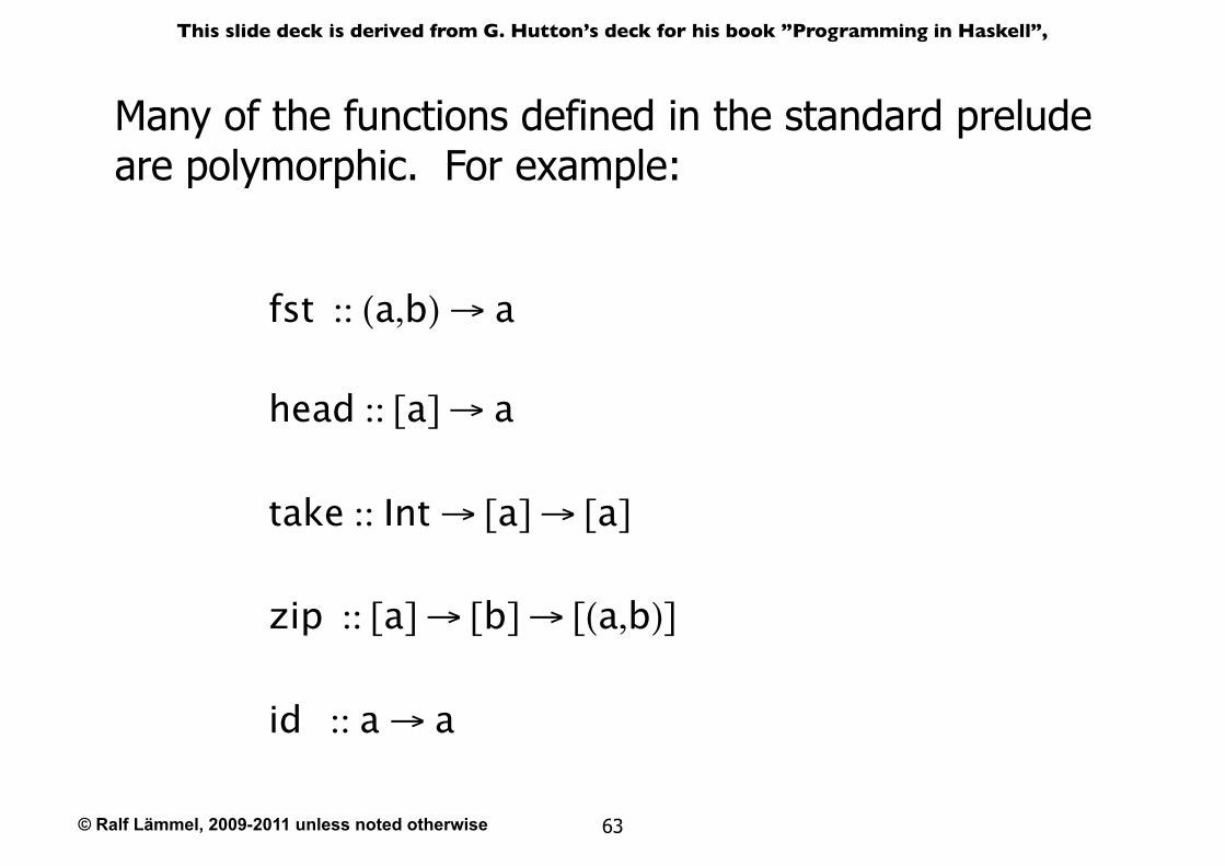
Many of the functions defined in the standard prelude are polymorphic. For example:
fst :: (a,b) → a
head :: [a] → a
take :: Int → [a] → [a]
zip :: [a] → [b] → [(a,b)]
id :: a → a
© Ralf Lämmel, 2009-2011 unless noted otherwise
This slide deck is derived from G. Hutton’s deck for his book ”Programming in Haskell”,
64
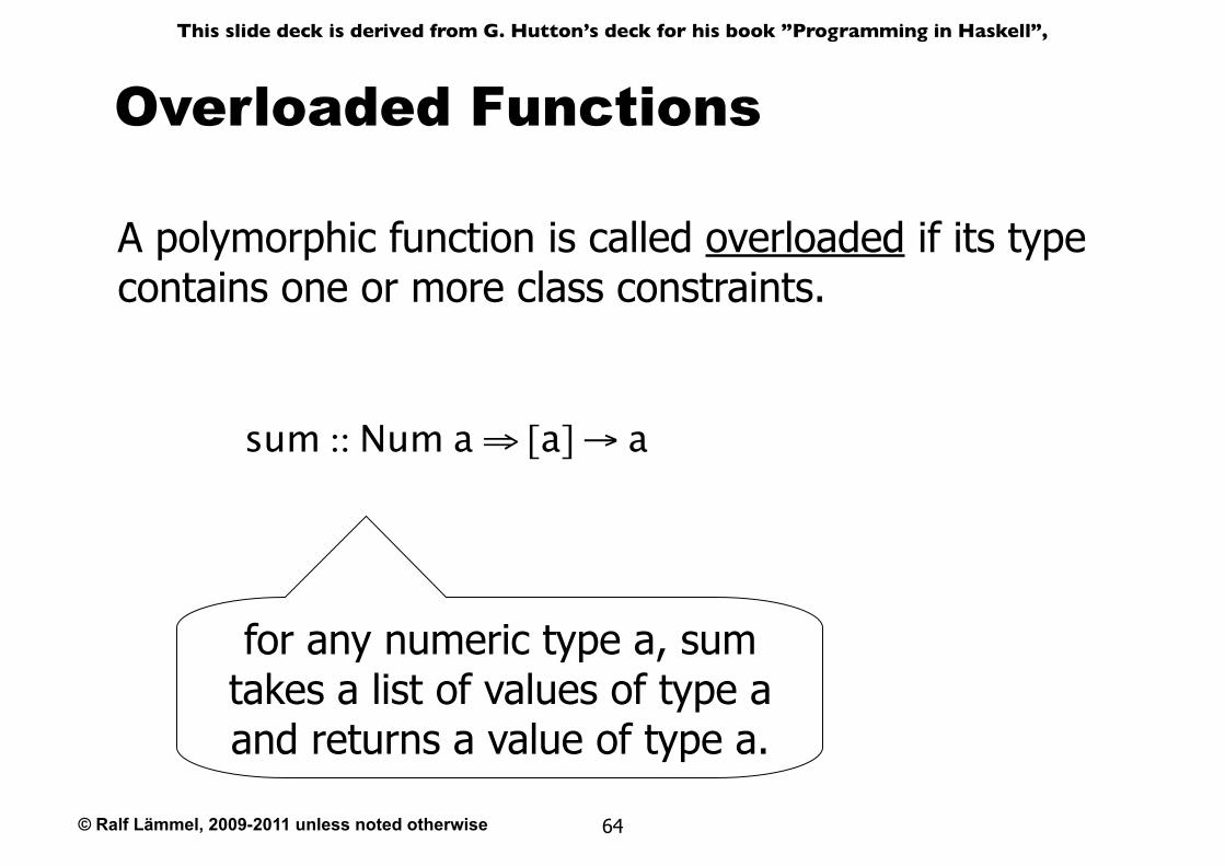
Overloaded Functions
A polymorphic function is called overloaded if its type contains one or more class constraints.
sum :: Num a ⇒ [a] → a
for any numeric type a, sum takes a list of values of type a and returns a value of type a.
© Ralf Lämmel, 2009-2011 unless noted otherwise
This slide deck is derived from G. Hutton’s deck for his book ”Programming in Haskell”,
65
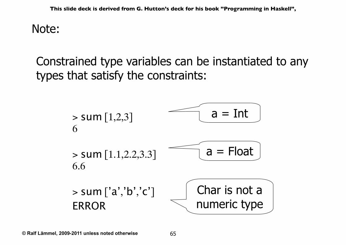
Constrained type variables can be instantiated to any types that satisfy the constraints:
Note:
> sum [1,2,3]6
> sum [1.1,2.2,3.3]6.6
> sum [’a’,’b’,’c’]ERROR
Char is not a numeric type
a = Int
a = Float
© Ralf Lämmel, 2009-2011 unless noted otherwise
This slide deck is derived from G. Hutton’s deck for his book ”Programming in Haskell”,
66
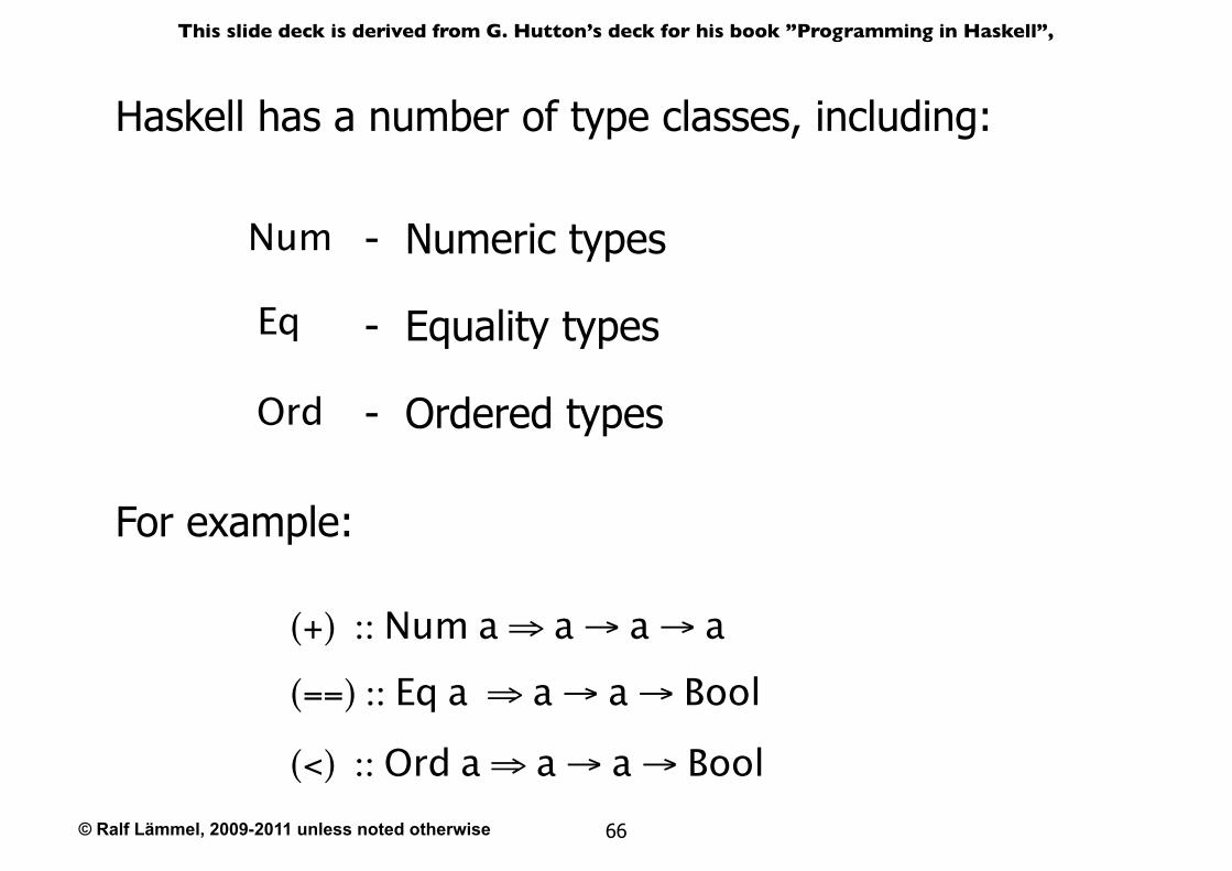
Num - Numeric types
Eq - Equality types
Ord - Ordered types
Haskell has a number of type classes, including:
For example:
(+) :: Num a ⇒ a → a → a (==) :: Eq a ⇒ a → a → Bool
(<) :: Ord a ⇒ a → a → Bool
© Ralf Lämmel, 2009-2011 unless noted otherwise
This slide deck is derived from G. Hutton’s deck for his book ”Programming in Haskell”,
67
Hints and Tips
★When stating the types of polymorphic functions that use numbers, equality or orderings, take care to include the necessary class constraints.
© Ralf Lämmel, 2009-2011 unless noted otherwise
This slide deck is derived from G. Hutton’s deck for his book ”Programming in Haskell”,
68
Exercises
[tail,init,reverse]
What is the type of the following value?(1)
© Ralf Lämmel, 2009-2011 unless noted otherwise
This slide deck is derived from G. Hutton’s deck for his book ”Programming in Haskell”,
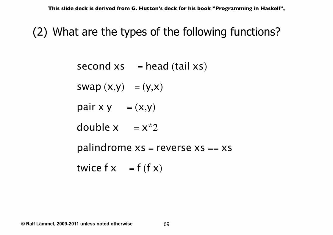
69
second xs = head (tail xs)
swap (x,y) = (y,x)
pair x y = (x,y)
double x = x*2
palindrome xs = reverse xs == xs
twice f x = f (f x)
What are the types of the following functions?(2)
© Ralf Lämmel, 2009-2011 unless noted otherwise
This slide deck is derived from G. Hutton’s deck for his book ”Programming in Haskell”,
70
Defining Functions
© Ralf Lämmel, 2009-2011 unless noted otherwise
This slide deck is derived from G. Hutton’s deck for his book ”Programming in Haskell”,
71
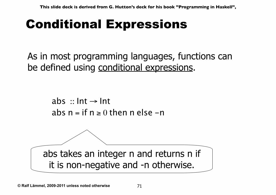
Conditional Expressions
As in most programming languages, functions can be defined using conditional expressions.
abs :: Int → Intabs n = if n ≥ 0 then n else -n
abs takes an integer n and returns n if it is non-negative and -n otherwise.
© Ralf Lämmel, 2009-2011 unless noted otherwise
This slide deck is derived from G. Hutton’s deck for his book ”Programming in Haskell”,
72
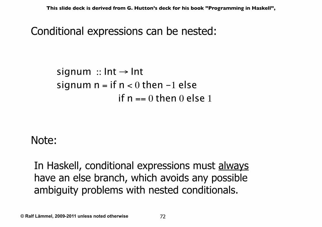
Conditional expressions can be nested:
signum :: Int → Intsignum n = if n < 0 then -1 else if n == 0 then 0 else 1
In Haskell, conditional expressions must always have an else branch, which avoids any possible ambiguity problems with nested conditionals.
Note:
© Ralf Lämmel, 2009-2011 unless noted otherwise
This slide deck is derived from G. Hutton’s deck for his book ”Programming in Haskell”,
73
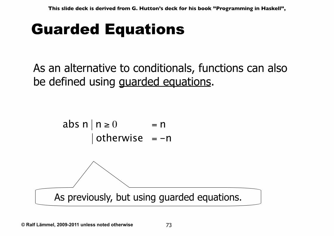
Guarded Equations
As an alternative to conditionals, functions can also be defined using guarded equations.
abs n | n ≥ 0 = n | otherwise = -n
As previously, but using guarded equations.
© Ralf Lämmel, 2009-2011 unless noted otherwise
This slide deck is derived from G. Hutton’s deck for his book ”Programming in Haskell”,
74
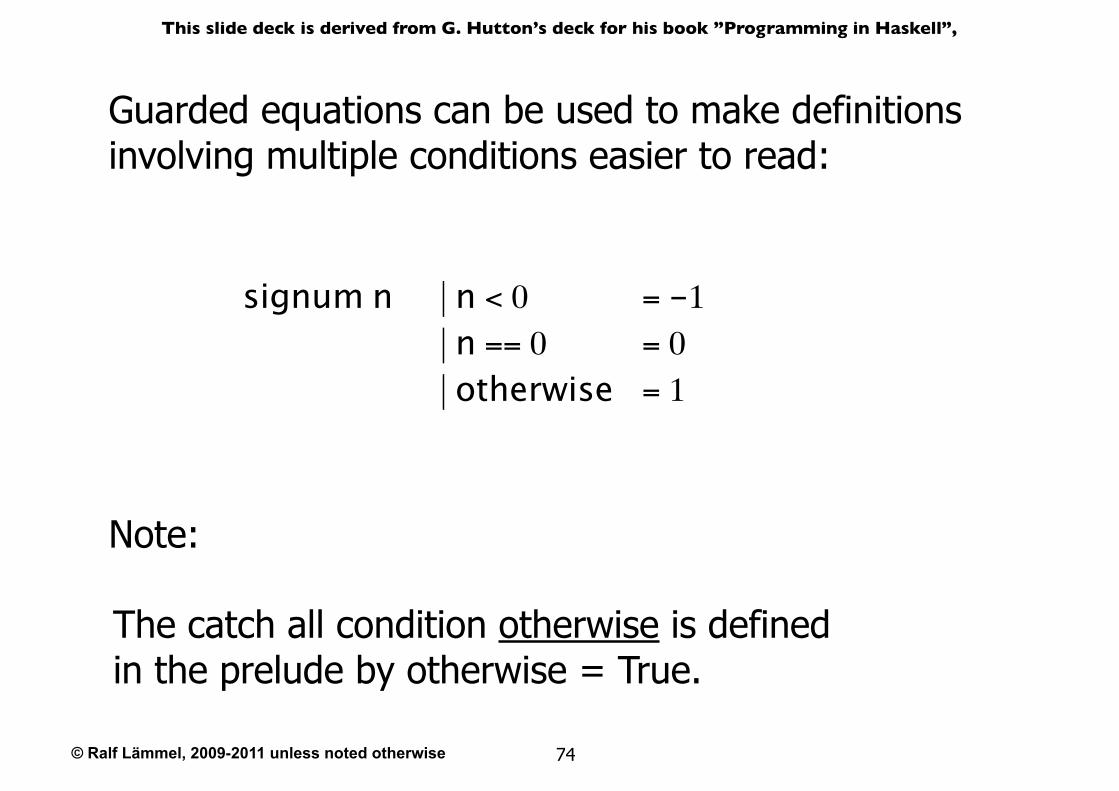
Guarded equations can be used to make definitions involving multiple conditions easier to read:
The catch all condition otherwise is defined in the prelude by otherwise = True.
Note:
signum n | n < 0 = -1 | n == 0 = 0 | otherwise = 1
© Ralf Lämmel, 2009-2011 unless noted otherwise
This slide deck is derived from G. Hutton’s deck for his book ”Programming in Haskell”,
75
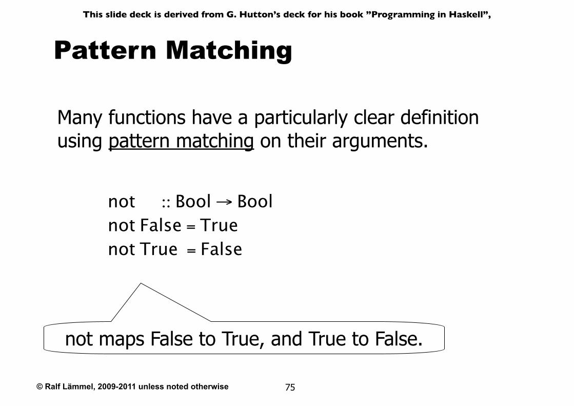
Pattern Matching
Many functions have a particularly clear definition using pattern matching on their arguments.
not :: Bool → Boolnot False = Truenot True = False
not maps False to True, and True to False.
© Ralf Lämmel, 2009-2011 unless noted otherwise
This slide deck is derived from G. Hutton’s deck for his book ”Programming in Haskell”,
76
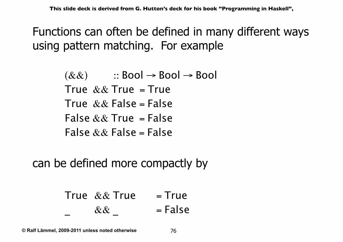
Functions can often be defined in many different ways using pattern matching. For example
(&&) :: Bool → Bool → BoolTrue && True = TrueTrue && False = FalseFalse && True = False False && False = False
True && True = True_ && _ = False
can be defined more compactly by
© Ralf Lämmel, 2009-2011 unless noted otherwise
This slide deck is derived from G. Hutton’s deck for his book ”Programming in Haskell”,
77
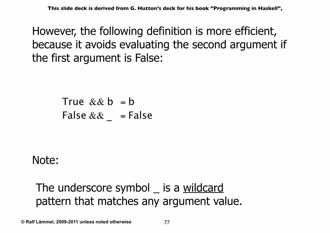
True && b = bFalse && _ = False
However, the following definition is more efficient, because it avoids evaluating the second argument if the first argument is False:
The underscore symbol _ is a wildcard pattern that matches any argument value.
Note:
© Ralf Lämmel, 2009-2011 unless noted otherwise
This slide deck is derived from G. Hutton’s deck for his book ”Programming in Haskell”,
78
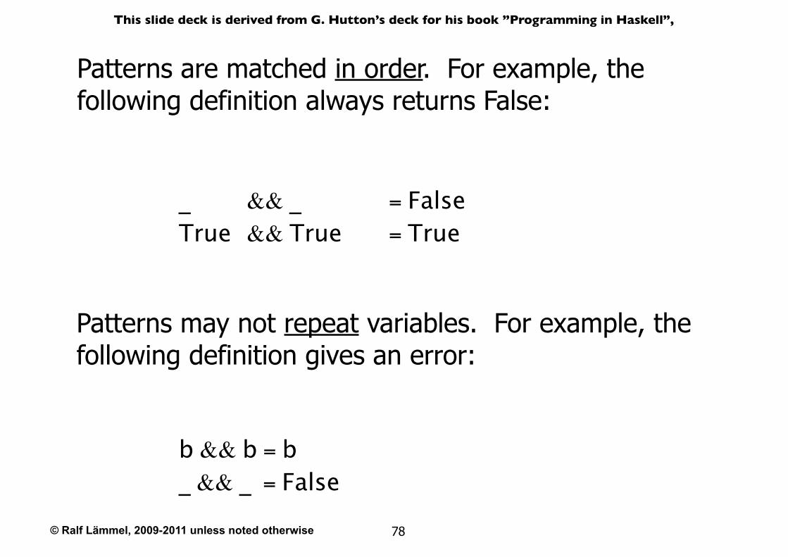
Patterns may not repeat variables. For example, the following definition gives an error:
b && b = b_ && _ = False
Patterns are matched in order. For example, the following definition always returns False:
_ && _ = FalseTrue && True = True
© Ralf Lämmel, 2009-2011 unless noted otherwise
This slide deck is derived from G. Hutton’s deck for his book ”Programming in Haskell”,
79
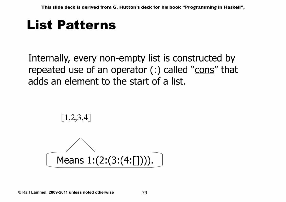
List Patterns
Internally, every non-empty list is constructed by repeated use of an operator (:) called “cons” that adds an element to the start of a list.
[1,2,3,4]
Means 1:(2:(3:(4:[]))).
© Ralf Lämmel, 2009-2011 unless noted otherwise
This slide deck is derived from G. Hutton’s deck for his book ”Programming in Haskell”,
80
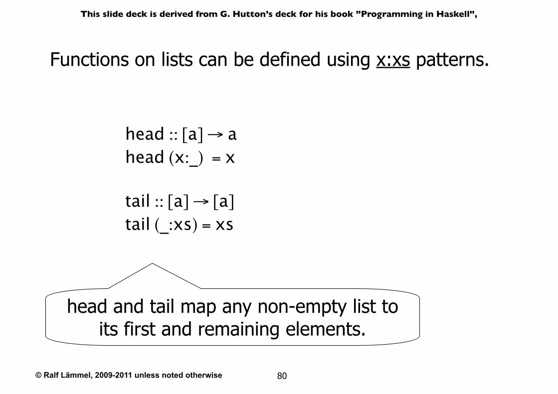
Functions on lists can be defined using x:xs patterns.
head :: [a] → ahead (x:_) = x
tail :: [a] → [a]tail (_:xs) = xs
head and tail map any non-empty list to its first and remaining elements.
© Ralf Lämmel, 2009-2011 unless noted otherwise
This slide deck is derived from G. Hutton’s deck for his book ”Programming in Haskell”,
81
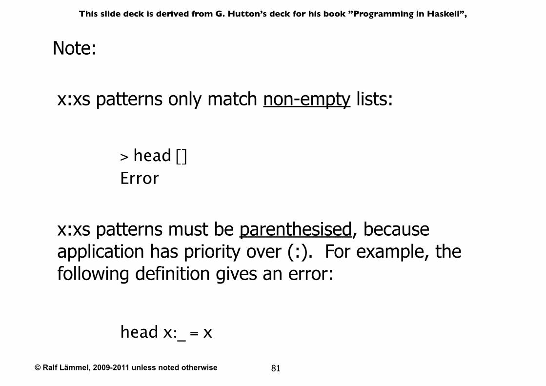
Note:
x:xs patterns must be parenthesised, because application has priority over (:). For example, the following definition gives an error:
x:xs patterns only match non-empty lists:
> head []Error
head x:_ = x
© Ralf Lämmel, 2009-2011 unless noted otherwise
This slide deck is derived from G. Hutton’s deck for his book ”Programming in Haskell”,
82
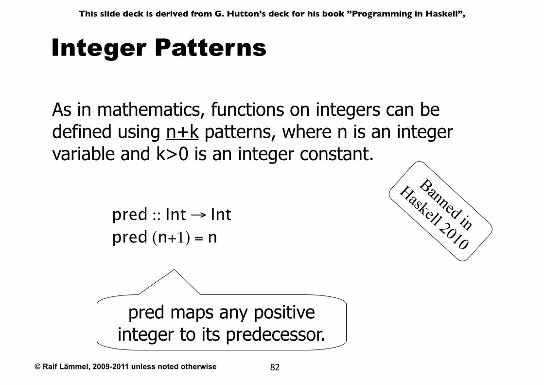
Integer Patterns
pred :: Int → Intpred (n+1) = n
As in mathematics, functions on integers can be defined using n+k patterns, where n is an integer variable and k>0 is an integer constant.
pred maps any positive integer to its predecessor.
Banned in
Haskell 2010
© Ralf Lämmel, 2009-2011 unless noted otherwise
This slide deck is derived from G. Hutton’s deck for his book ”Programming in Haskell”,
83
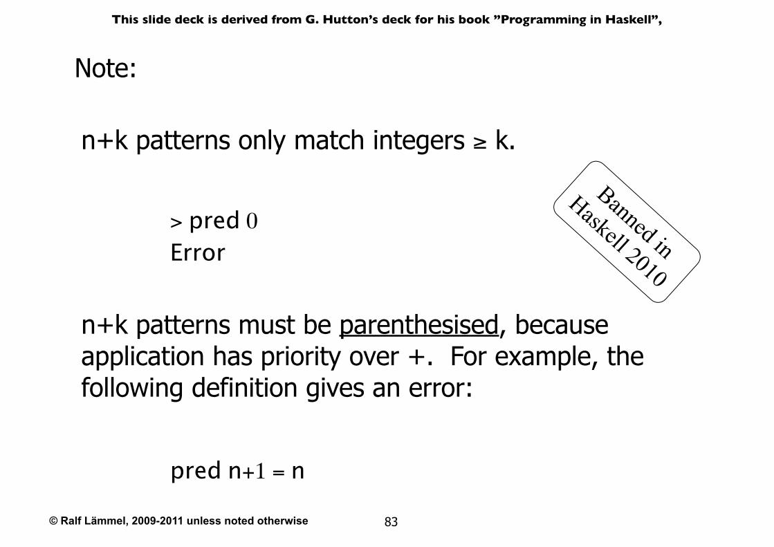
Note:
n+k patterns must be parenthesised, because application has priority over +. For example, the following definition gives an error:
n+k patterns only match integers ≥ k.
> pred 0Error
pred n+1 = n
Banned in
Haskell 2010
© Ralf Lämmel, 2009-2011 unless noted otherwise
This slide deck is derived from G. Hutton’s deck for his book ”Programming in Haskell”,
84
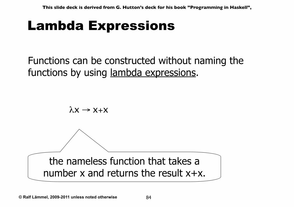
Lambda Expressions
Functions can be constructed without naming the functions by using lambda expressions.
λx → x+x
the nameless function that takes a number x and returns the result x+x.
© Ralf Lämmel, 2009-2011 unless noted otherwise
This slide deck is derived from G. Hutton’s deck for his book ”Programming in Haskell”,
85
๏The symbol λ is the Greek letter lambda, and is typed at the keyboard as a backslash \.
๏In mathematics, nameless functions are usually denoted using the a symbol, as in x a x+x.
๏In Haskell, the use of the λ symbol for nameless functions comes from the lambda calculus, the theory of functions on which Haskell is based.
Note:
© Ralf Lämmel, 2009-2011 unless noted otherwise
This slide deck is derived from G. Hutton’s deck for his book ”Programming in Haskell”,
86
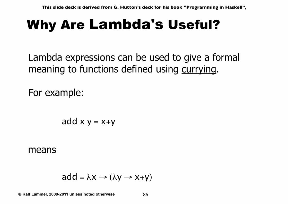
Why Are Lambda's Useful?
Lambda expressions can be used to give a formal meaning to functions defined using currying.
For example:
add x y = x+y
add = λx → (λy → x+y)
means
© Ralf Lämmel, 2009-2011 unless noted otherwise
This slide deck is derived from G. Hutton’s deck for his book ”Programming in Haskell”,
87
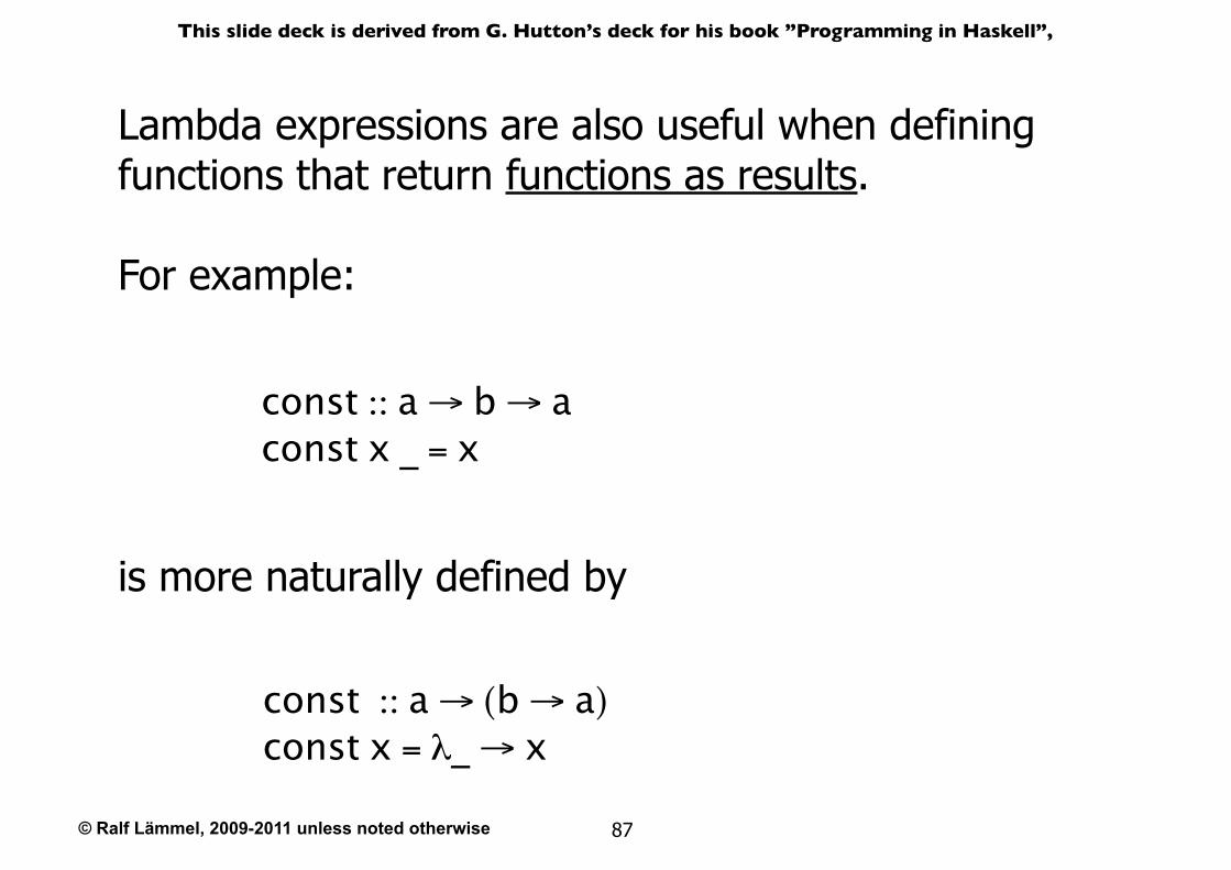
const :: a → b → aconst x _ = x
is more naturally defined by
const :: a → (b → a)const x = λ_ → x
Lambda expressions are also useful when defining functions that return functions as results.
For example:
© Ralf Lämmel, 2009-2011 unless noted otherwise
This slide deck is derived from G. Hutton’s deck for his book ”Programming in Haskell”,
88
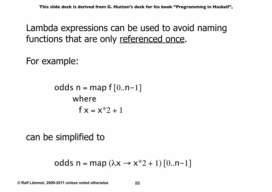
odds n = map f [0..n-1] where f x = x*2 + 1
can be simplified to
odds n = map (λx → x*2 + 1) [0..n-1]
Lambda expressions can be used to avoid naming functions that are only referenced once.
For example:
© Ralf Lämmel, 2009-2011 unless noted otherwise
This slide deck is derived from G. Hutton’s deck for his book ”Programming in Haskell”,
89
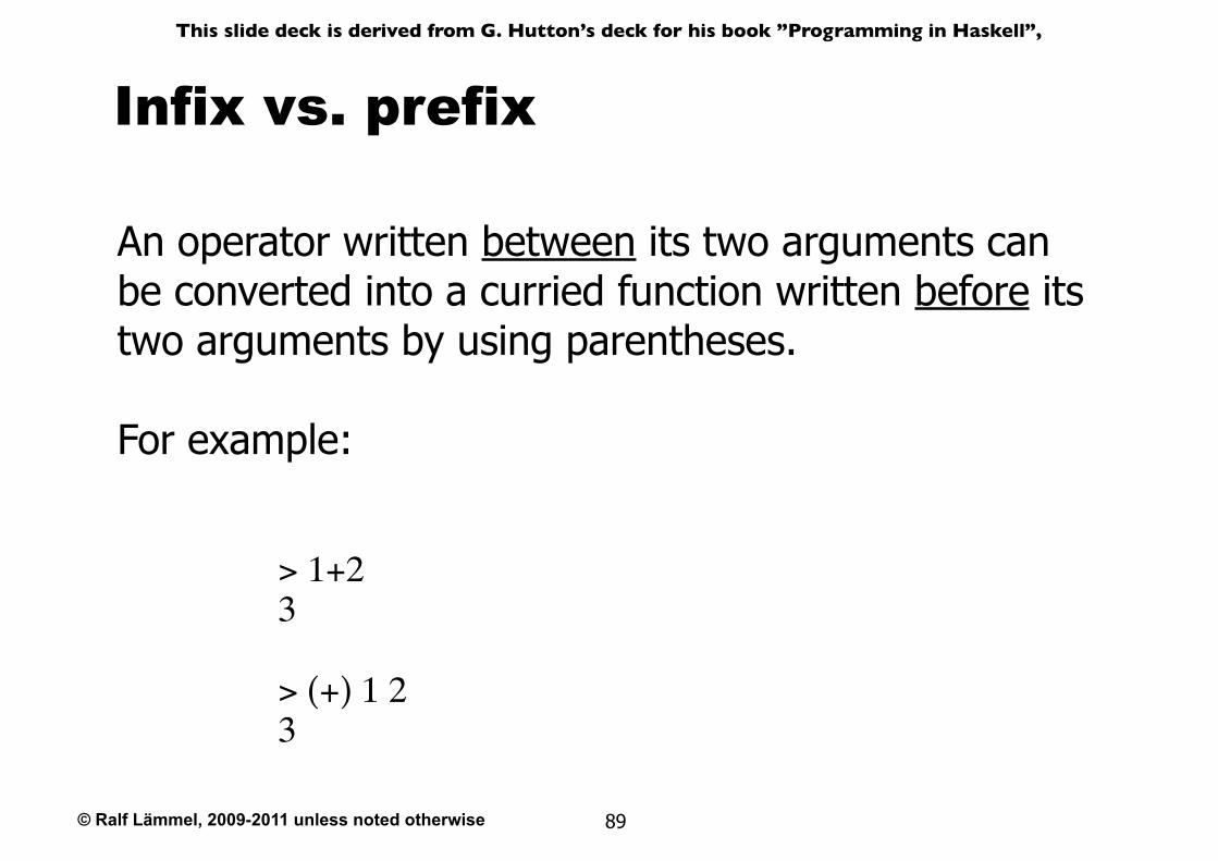
Infix vs. prefix
An operator written between its two arguments can be converted into a curried function written before its two arguments by using parentheses.
For example:
> 1+23
> (+) 1 23
© Ralf Lämmel, 2009-2011 unless noted otherwise
This slide deck is derived from G. Hutton’s deck for his book ”Programming in Haskell”,
90
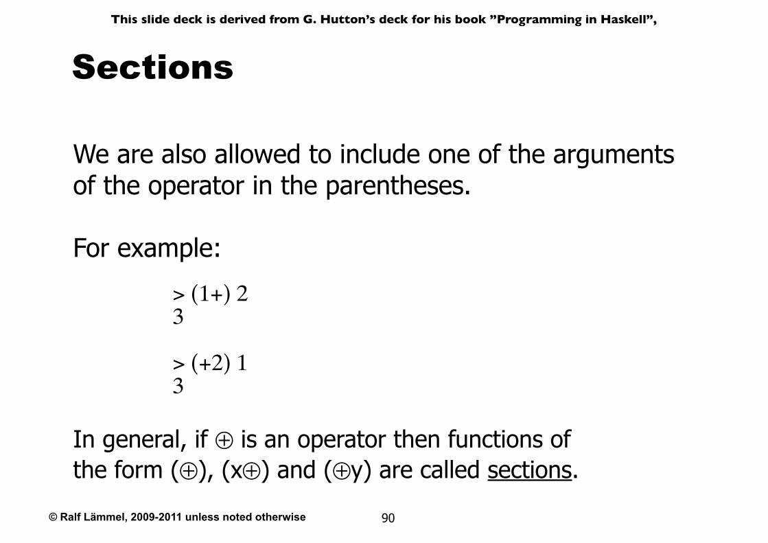
We are also allowed to include one of the arguments of the operator in the parentheses.
For example:
> (1+) 23
> (+2) 13
In general, if ⊕ is an operator then functions of the form (⊕), (x⊕) and (⊕y) are called sections.
Sections
© Ralf Lämmel, 2009-2011 unless noted otherwise
This slide deck is derived from G. Hutton’s deck for his book ”Programming in Haskell”,
91
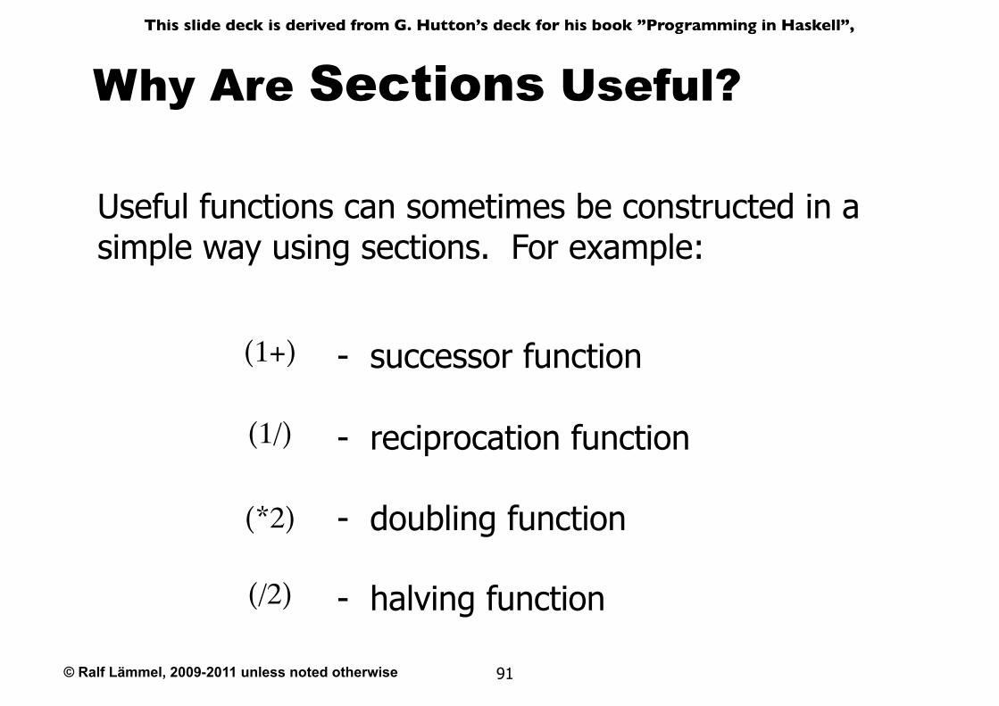
Why Are Sections Useful?
Useful functions can sometimes be constructed in a simple way using sections. For example:
- successor function
- reciprocation function
- doubling function
- halving function
(1+)
(*2)
(/2)
(1/)
© Ralf Lämmel, 2009-2011 unless noted otherwise
This slide deck is derived from G. Hutton’s deck for his book ”Programming in Haskell”,
92
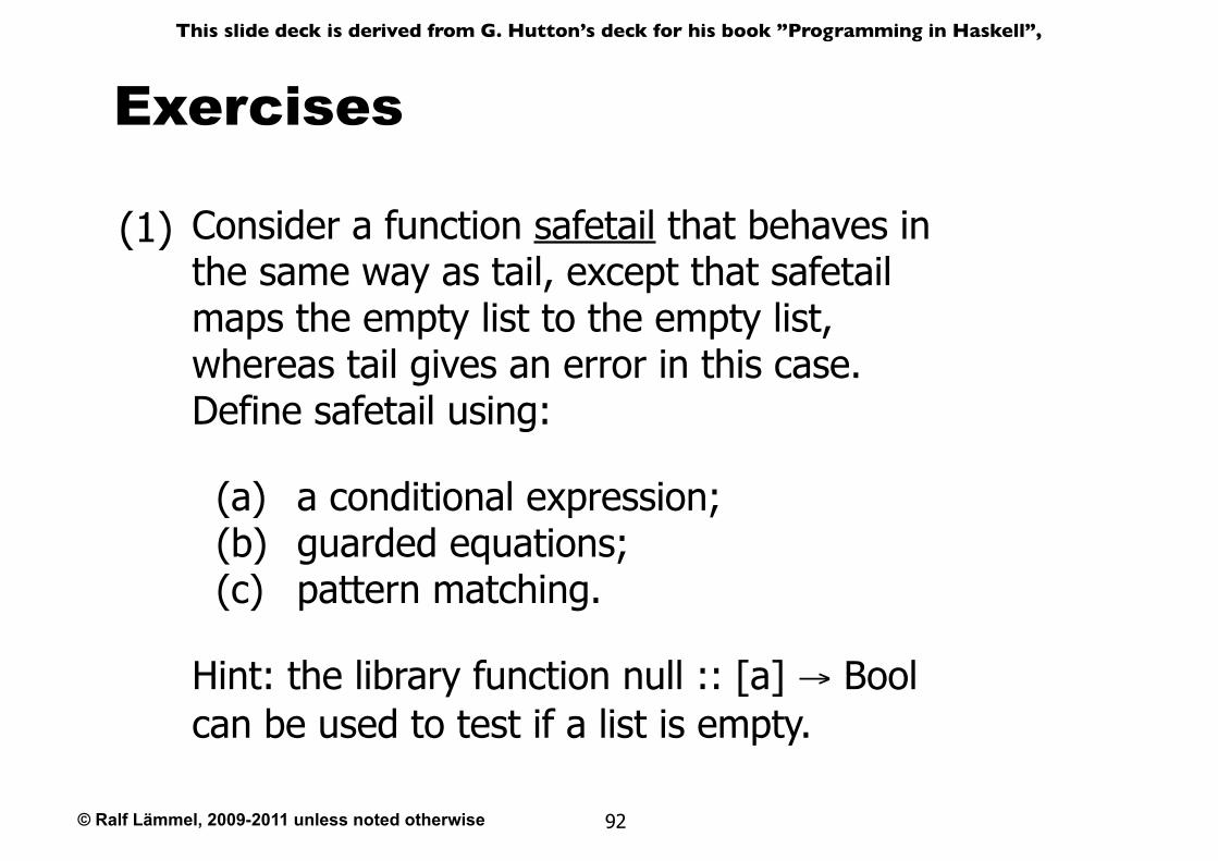
Exercises
Consider a function safetail that behaves in the same way as tail, except that safetail maps the empty list to the empty list, whereas tail gives an error in this case. Define safetail using:
(a) a conditional expression; (b) guarded equations; (c) pattern matching.
Hint: the library function null :: [a] → Bool can be used to test if a list is empty.
(1)
© Ralf Lämmel, 2009-2011 unless noted otherwise
This slide deck is derived from G. Hutton’s deck for his book ”Programming in Haskell”,
93
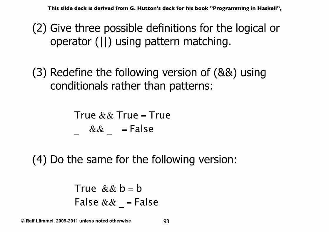
Give three possible definitions for the logical or operator (||) using pattern matching.
(2)
Redefine the following version of (&&) using conditionals rather than patterns:
(3)
True && True = True_ && _ = False
Do the same for the following version:(4)
True && b = bFalse && _ = False
© Ralf Lämmel, 2009-2011 unless noted otherwise
This slide deck is derived from G. Hutton’s deck for his book ”Programming in Haskell”,
94
List Comprehensions
© Ralf Lämmel, 2009-2011 unless noted otherwise
This slide deck is derived from G. Hutton’s deck for his book ”Programming in Haskell”,
95
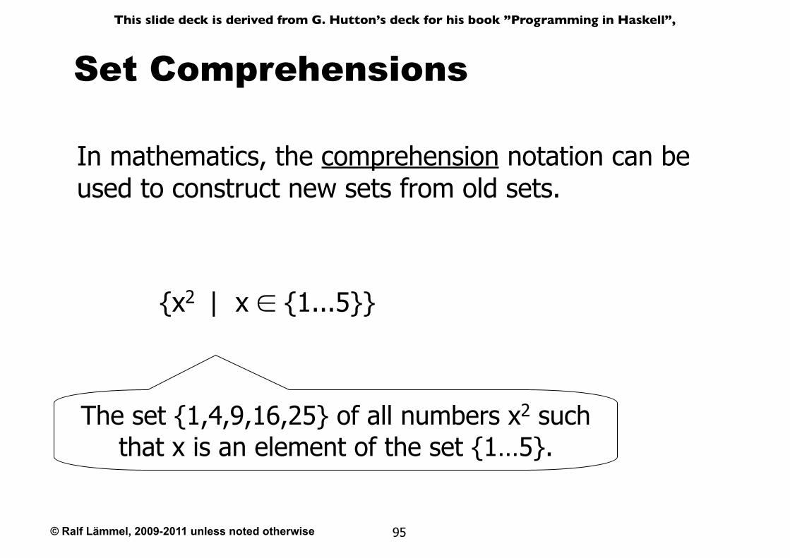
Set Comprehensions
In mathematics, the comprehension notation can be used to construct new sets from old sets.
{x2 | x ∈ {1...5}}
The set {1,4,9,16,25} of all numbers x2 such that x is an element of the set {1…5}.
© Ralf Lämmel, 2009-2011 unless noted otherwise
This slide deck is derived from G. Hutton’s deck for his book ”Programming in Haskell”,
96
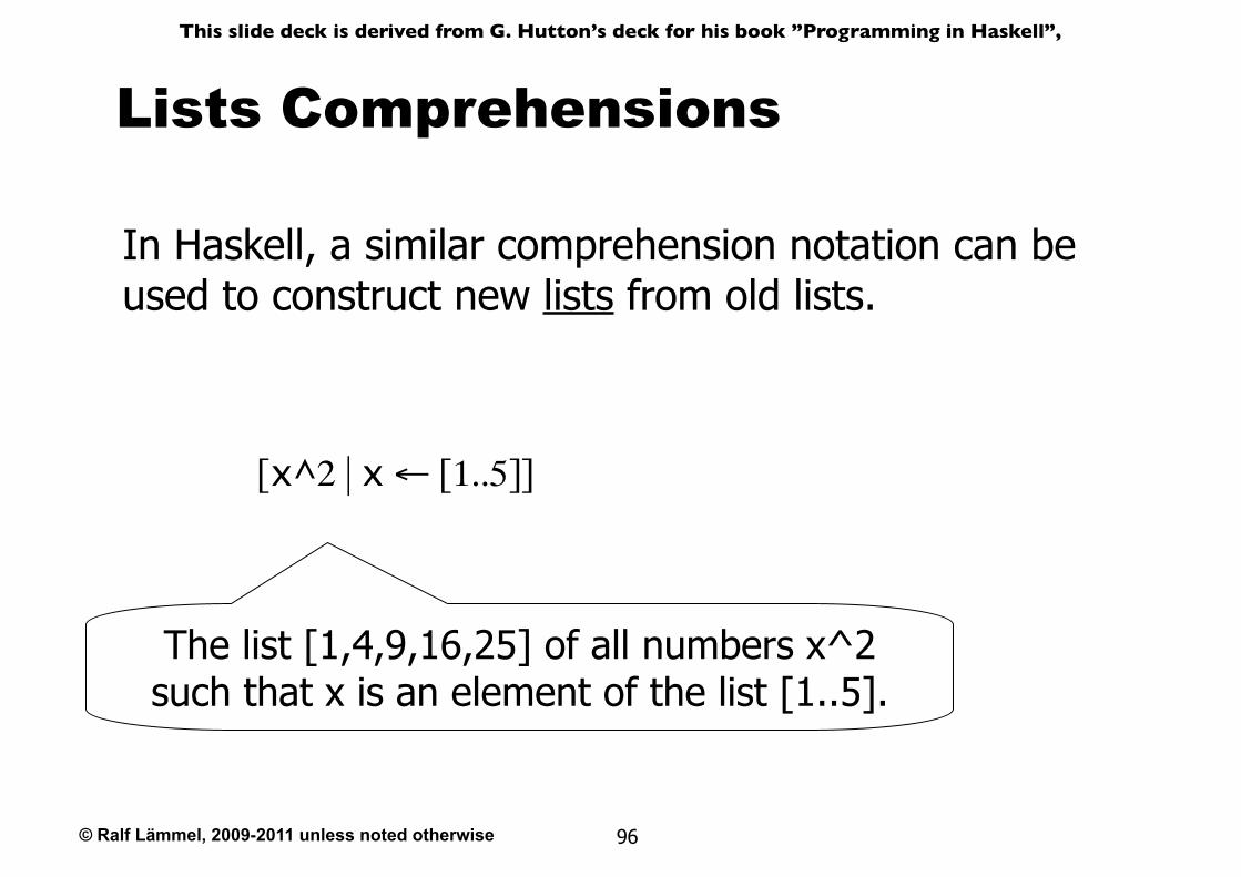
Lists Comprehensions
In Haskell, a similar comprehension notation can be used to construct new lists from old lists.
[x^2 | x ← [1..5]]
The list [1,4,9,16,25] of all numbers x^2
such that x is an element of the list [1..5].
© Ralf Lämmel, 2009-2011 unless noted otherwise
This slide deck is derived from G. Hutton’s deck for his book ”Programming in Haskell”,
97
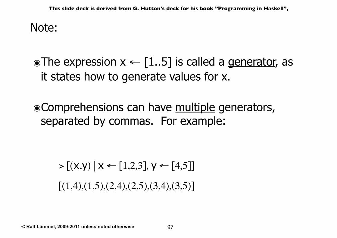
Note:
๏The expression x ← [1..5] is called a generator, as it states how to generate values for x.
๏Comprehensions can have multiple generators, separated by commas. For example:
> [(x,y) | x ← [1,2,3], y ← [4,5]]
[(1,4),(1,5),(2,4),(2,5),(3,4),(3,5)]
© Ralf Lämmel, 2009-2011 unless noted otherwise
This slide deck is derived from G. Hutton’s deck for his book ”Programming in Haskell”,
98
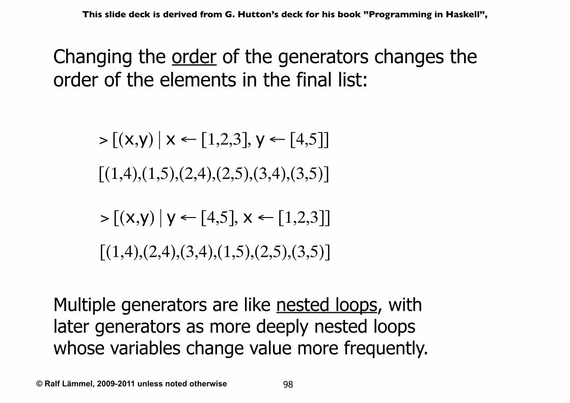
Changing the order of the generators changes the order of the elements in the final list:
> [(x,y) | y ← [4,5], x ← [1,2,3]]
[(1,4),(2,4),(3,4),(1,5),(2,5),(3,5)]
Multiple generators are like nested loops, with later generators as more deeply nested loops whose variables change value more frequently.
> [(x,y) | x ← [1,2,3], y ← [4,5]]
[(1,4),(1,5),(2,4),(2,5),(3,4),(3,5)]
© Ralf Lämmel, 2009-2011 unless noted otherwise
This slide deck is derived from G. Hutton’s deck for his book ”Programming in Haskell”,
99
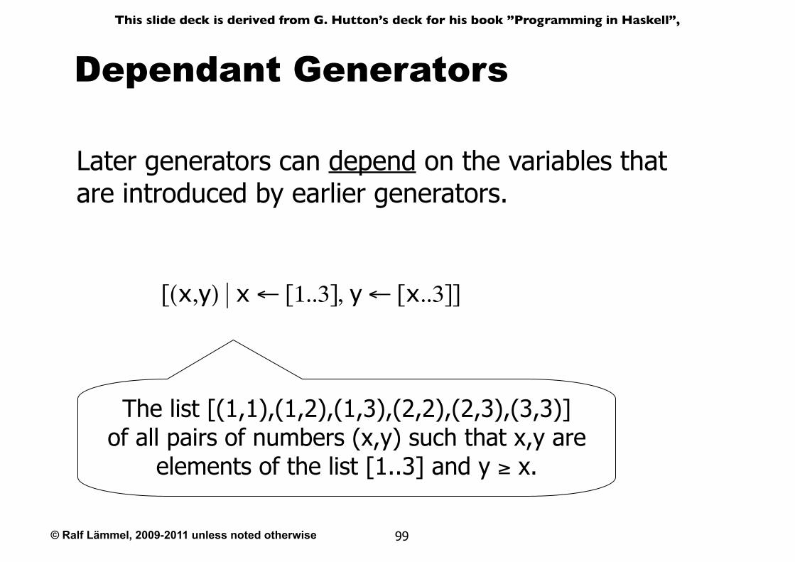
Dependant Generators
Later generators can depend on the variables that are introduced by earlier generators.
[(x,y) | x ← [1..3], y ← [x..3]]
The list [(1,1),(1,2),(1,3),(2,2),(2,3),(3,3)]of all pairs of numbers (x,y) such that x,y are
elements of the list [1..3] and y ≥ x.
© Ralf Lämmel, 2009-2011 unless noted otherwise
This slide deck is derived from G. Hutton’s deck for his book ”Programming in Haskell”,
100
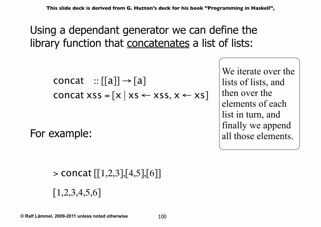
Using a dependant generator we can define the library function that concatenates a list of lists:
concat :: [[a]] → [a]
concat xss = [x | xs ← xss, x ← xs]
For example:
> concat [[1,2,3],[4,5],[6]]
[1,2,3,4,5,6]
We iterate over the lists of lists, and then over the elements of each list in turn, and finally we append all those elements.
© Ralf Lämmel, 2009-2011 unless noted otherwise
This slide deck is derived from G. Hutton’s deck for his book ”Programming in Haskell”,
101
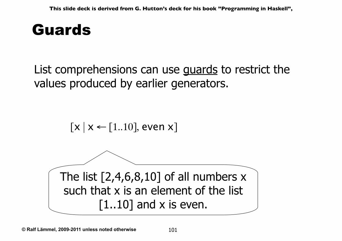
Guards
List comprehensions can use guards to restrict the values produced by earlier generators.
[x | x ← [1..10], even x]
The list [2,4,6,8,10] of all numbers x such that x is an element of the list
[1..10] and x is even.
© Ralf Lämmel, 2009-2011 unless noted otherwise
This slide deck is derived from G. Hutton’s deck for his book ”Programming in Haskell”,
102
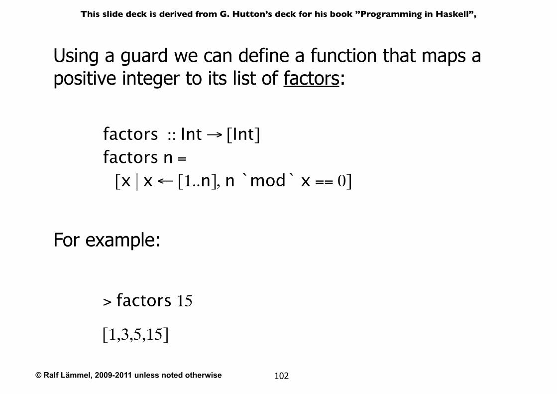
factors :: Int → [Int]factors n = [x | x ← [1..n], n `mod` x == 0]
Using a guard we can define a function that maps a positive integer to its list of factors:
For example:
> factors 15
[1,3,5,15]
© Ralf Lämmel, 2009-2011 unless noted otherwise
This slide deck is derived from G. Hutton’s deck for his book ”Programming in Haskell”,
103
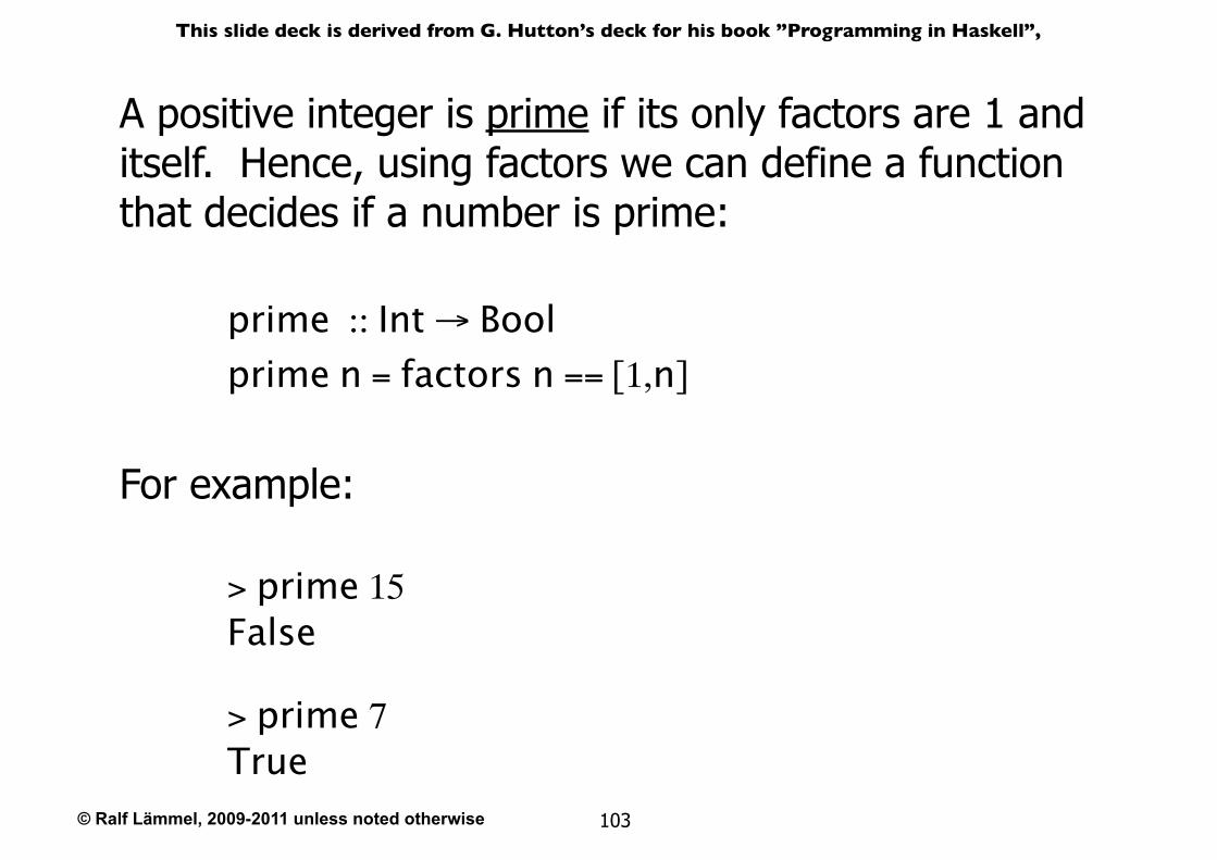
A positive integer is prime if its only factors are 1 and itself. Hence, using factors we can define a function that decides if a number is prime:
prime :: Int → Boolprime n = factors n == [1,n]
For example:
> prime 15False
> prime 7True
© Ralf Lämmel, 2009-2011 unless noted otherwise
This slide deck is derived from G. Hutton’s deck for his book ”Programming in Haskell”,
104
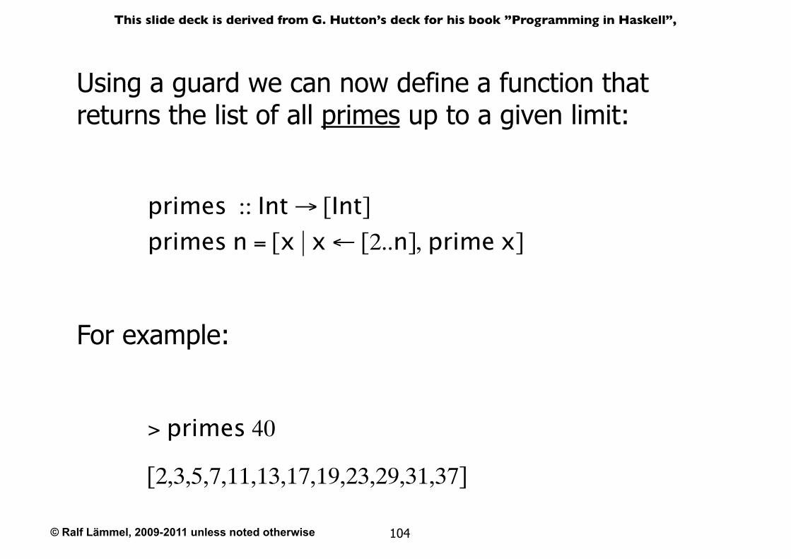
Using a guard we can now define a function that returns the list of all primes up to a given limit:
primes :: Int → [Int]primes n = [x | x ← [2..n], prime x]
For example:
> primes 40
[2,3,5,7,11,13,17,19,23,29,31,37]
© Ralf Lämmel, 2009-2011 unless noted otherwise
This slide deck is derived from G. Hutton’s deck for his book ”Programming in Haskell”,
105
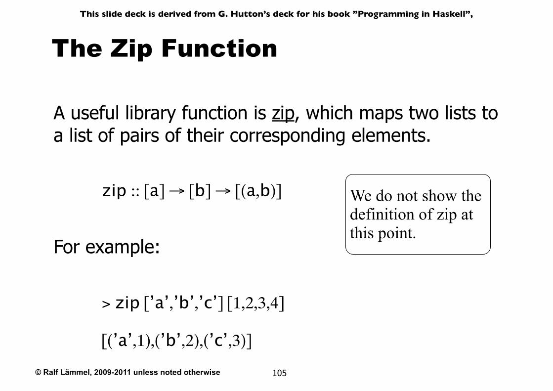
The Zip Function
A useful library function is zip, which maps two lists to a list of pairs of their corresponding elements.
zip :: [a] → [b] → [(a,b)]
For example:
> zip [’a’,’b’,’c’] [1,2,3,4]
[(’a’,1),(’b’,2),(’c’,3)]
We do not show the definition of zip at this point.
© Ralf Lämmel, 2009-2011 unless noted otherwise
This slide deck is derived from G. Hutton’s deck for his book ”Programming in Haskell”,
106
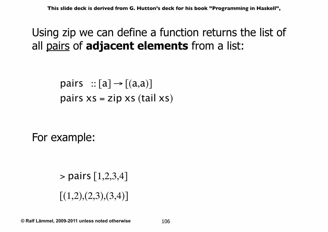
Using zip we can define a function returns the list of all pairs of adjacent elements from a list:
For example:
pairs :: [a] → [(a,a)]
pairs xs = zip xs (tail xs)
> pairs [1,2,3,4]
[(1,2),(2,3),(3,4)]
© Ralf Lämmel, 2009-2011 unless noted otherwise
This slide deck is derived from G. Hutton’s deck for his book ”Programming in Haskell”,
107
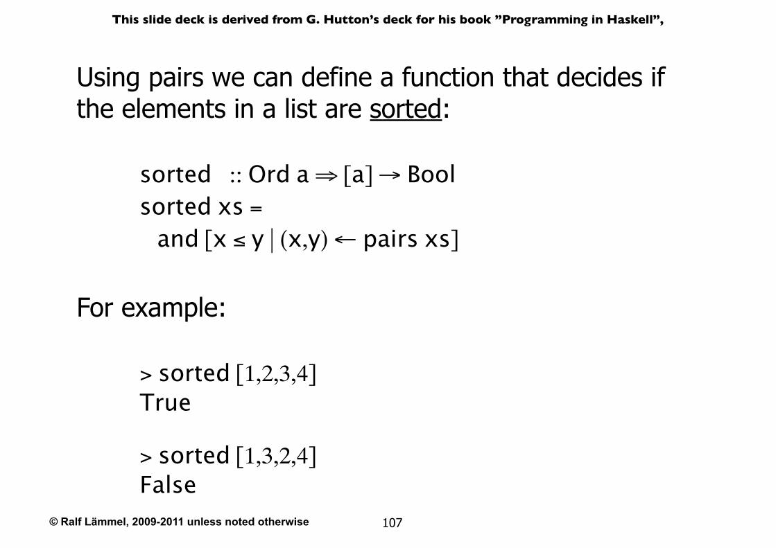
Using pairs we can define a function that decides if the elements in a list are sorted:
For example:
sorted :: Ord a ⇒ [a] → Boolsorted xs = and [x ≤ y | (x,y) ← pairs xs]
> sorted [1,2,3,4]True
> sorted [1,3,2,4]False
© Ralf Lämmel, 2009-2011 unless noted otherwise
This slide deck is derived from G. Hutton’s deck for his book ”Programming in Haskell”,
108
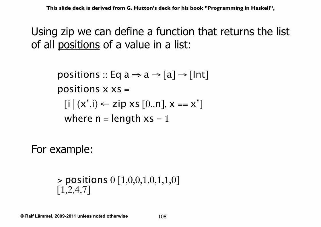
Using zip we can define a function that returns the list of all positions of a value in a list:
positions :: Eq a ⇒ a → [a] → [Int]positions x xs =
[i | (x’,i) ← zip xs [0..n], x == x’] where n = length xs - 1
For example:
> positions 0 [1,0,0,1,0,1,1,0][1,2,4,7]
© Ralf Lämmel, 2009-2011 unless noted otherwise
This slide deck is derived from G. Hutton’s deck for his book ”Programming in Haskell”,
109
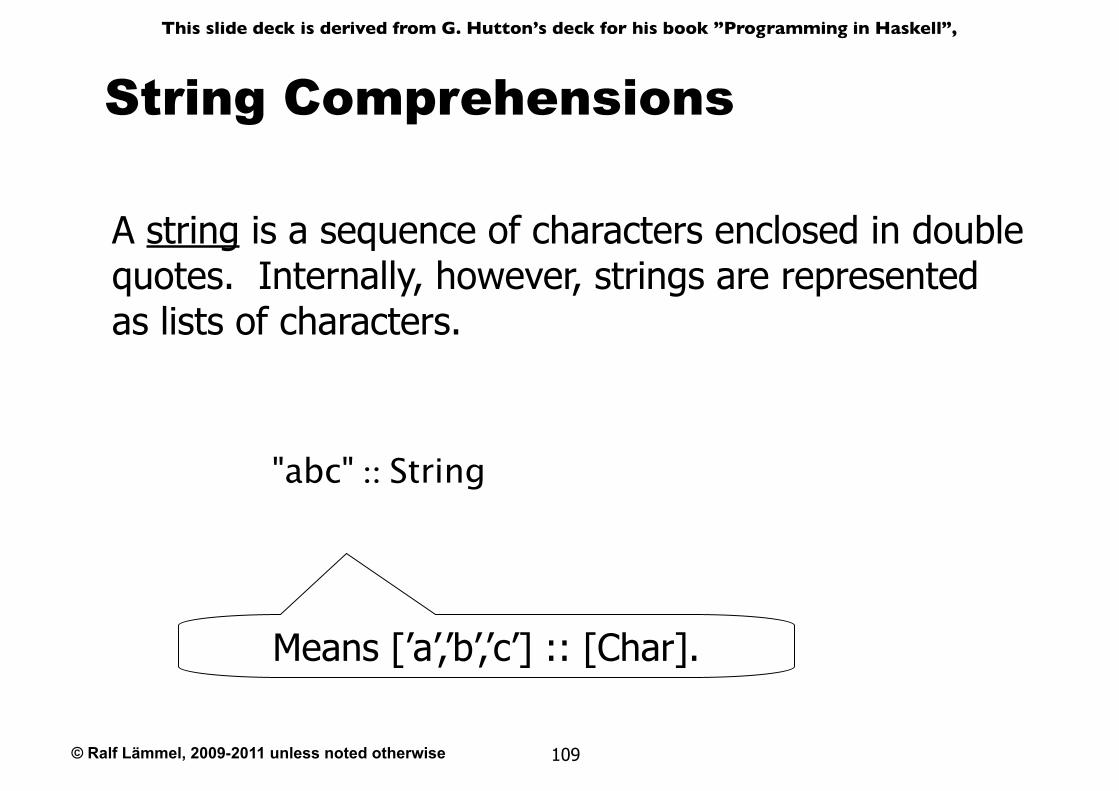
String Comprehensions
A string is a sequence of characters enclosed in double quotes. Internally, however, strings are represented as lists of characters.
"abc" :: String
Means [’a’,’b’,’c’] :: [Char].
© Ralf Lämmel, 2009-2011 unless noted otherwise
This slide deck is derived from G. Hutton’s deck for his book ”Programming in Haskell”,
110
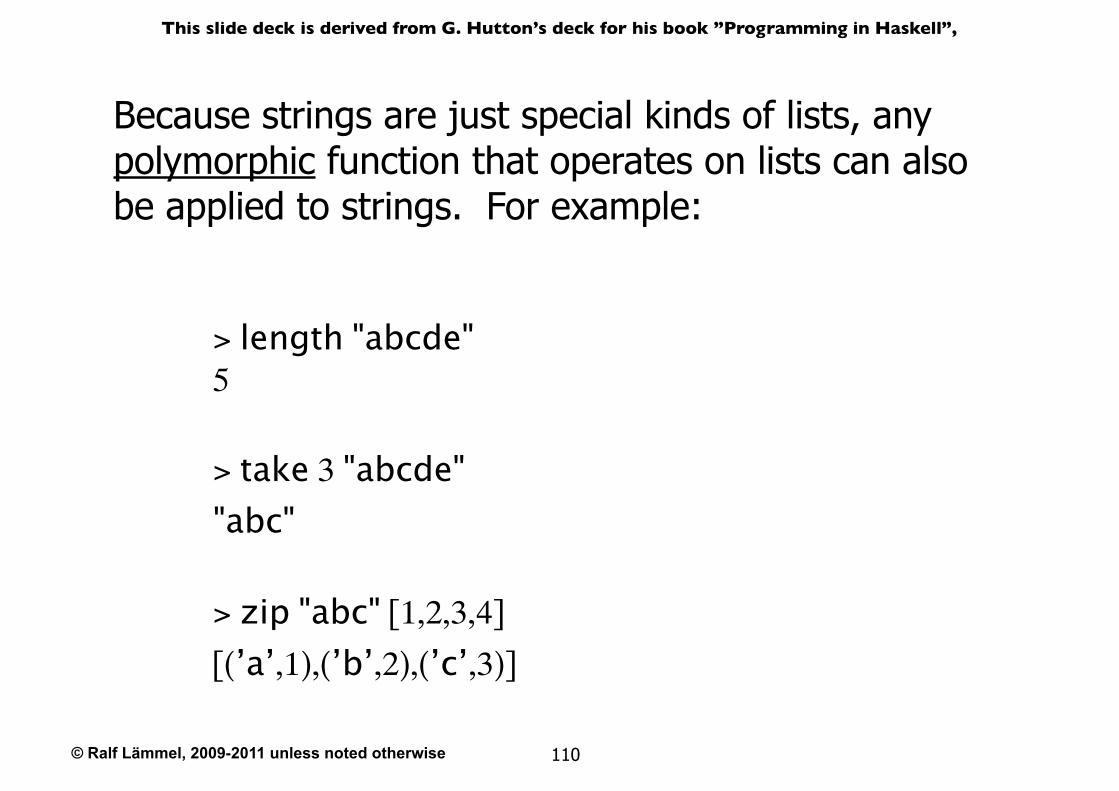
Because strings are just special kinds of lists, any polymorphic function that operates on lists can also be applied to strings. For example:
> length "abcde"5
> take 3 "abcde""abc"
> zip "abc" [1,2,3,4]
[(’a’,1),(’b’,2),(’c’,3)]
© Ralf Lämmel, 2009-2011 unless noted otherwise
This slide deck is derived from G. Hutton’s deck for his book ”Programming in Haskell”,
111
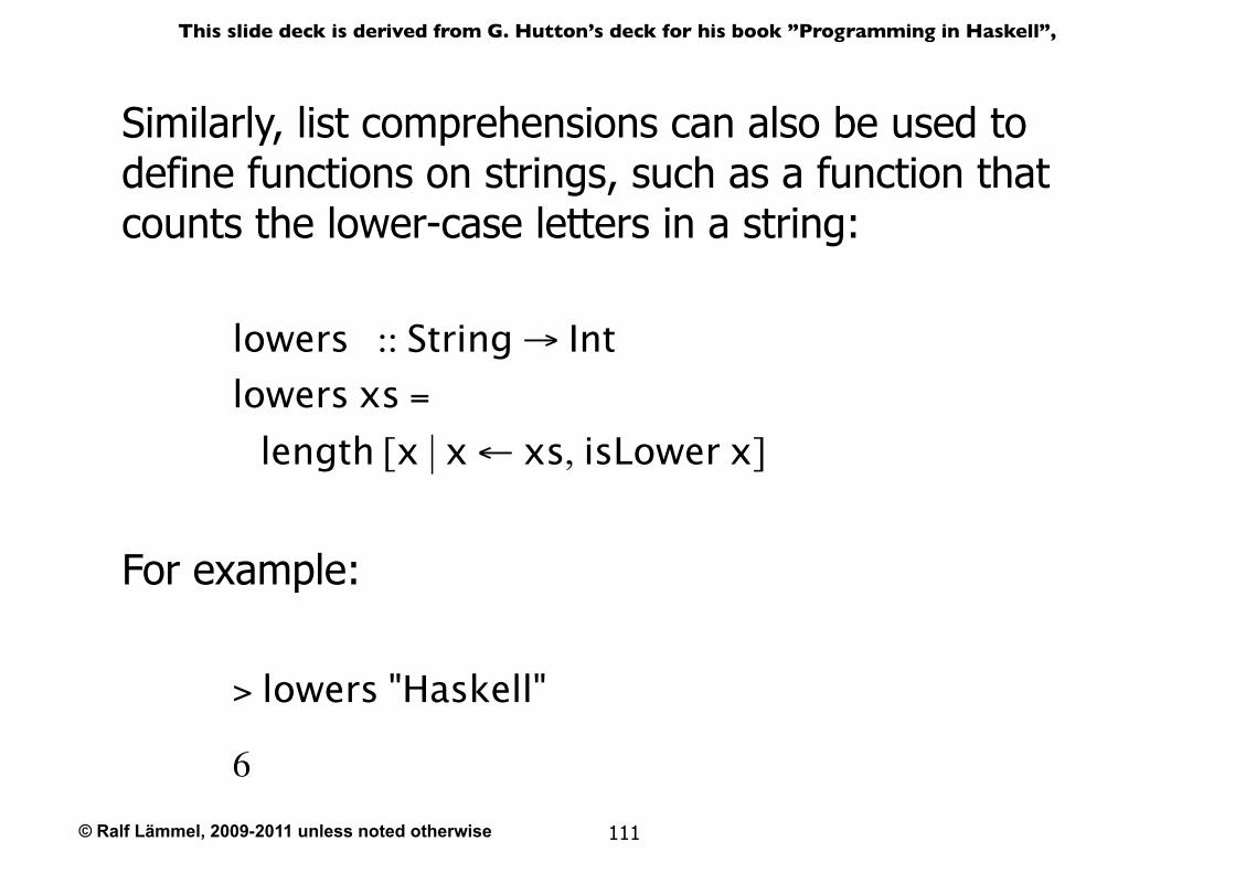
Similarly, list comprehensions can also be used to define functions on strings, such as a function that counts the lower-case letters in a string:
lowers :: String → Intlowers xs =
length [x | x ← xs, isLower x]
For example:
> lowers "Haskell"
6
© Ralf Lämmel, 2009-2011 unless noted otherwise
This slide deck is derived from G. Hutton’s deck for his book ”Programming in Haskell”,
112
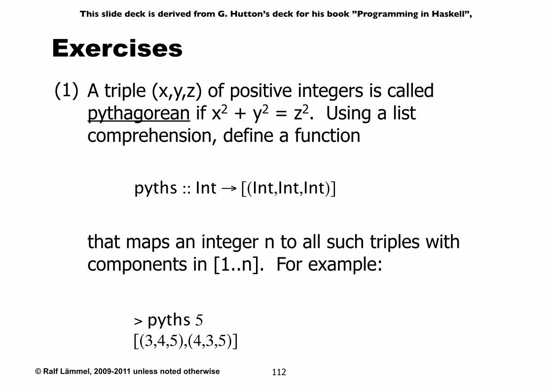
ExercisesA triple (x,y,z) of positive integers is called pythagorean if x2 + y2 = z2. Using a list comprehension, define a function
(1)
pyths :: Int → [(Int,Int,Int)]
that maps an integer n to all such triples with components in [1..n]. For example:
> pyths 5[(3,4,5),(4,3,5)]
© Ralf Lämmel, 2009-2011 unless noted otherwise
This slide deck is derived from G. Hutton’s deck for his book ”Programming in Haskell”,
113
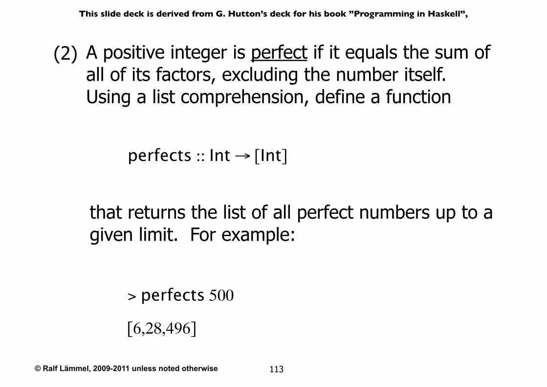
A positive integer is perfect if it equals the sum of all of its factors, excluding the number itself. Using a list comprehension, define a function
(2)
perfects :: Int → [Int]
that returns the list of all perfect numbers up to a given limit. For example:
> perfects 500
[6,28,496]
© Ralf Lämmel, 2009-2011 unless noted otherwise
This slide deck is derived from G. Hutton’s deck for his book ”Programming in Haskell”,
114
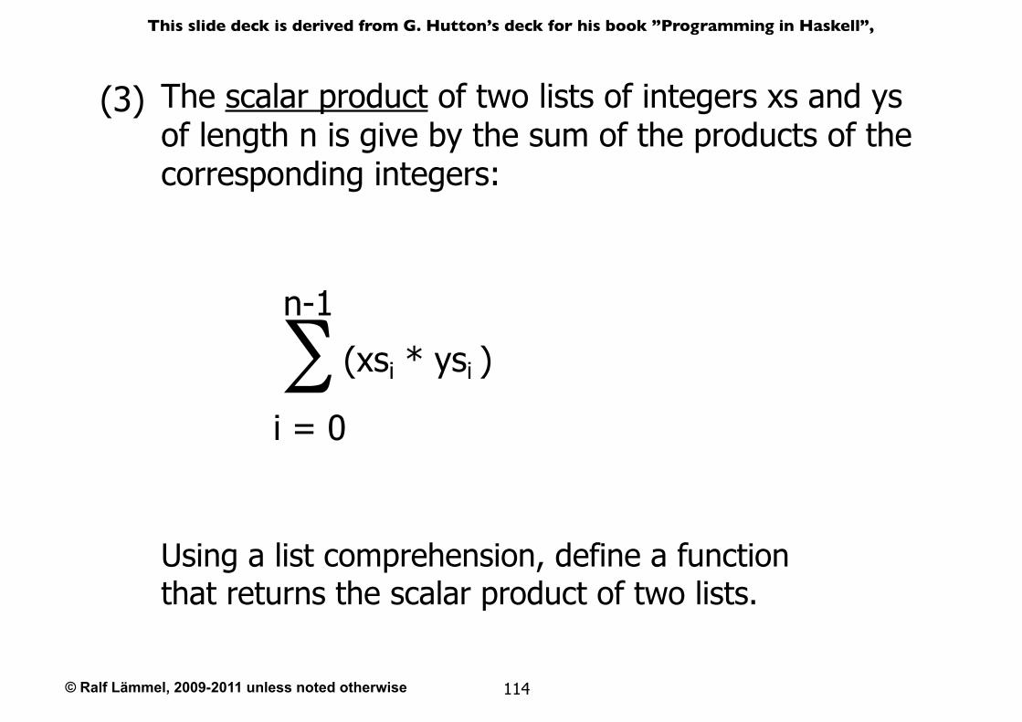
(xsi * ysi )∑i = 0
n-1
Using a list comprehension, define a function that returns the scalar product of two lists.
The scalar product of two lists of integers xs and ys of length n is give by the sum of the products of the corresponding integers:
(3)
© Ralf Lämmel, 2009-2011 unless noted otherwise
This slide deck is derived from G. Hutton’s deck for his book ”Programming in Haskell”,
115
Recursive Functions
© Ralf Lämmel, 2009-2011 unless noted otherwise
This slide deck is derived from G. Hutton’s deck for his book ”Programming in Haskell”,
116
Introduction
As we have seen, many functions can naturally be defined in terms of other functions.
factorial :: Int → Intfactorial n = product [1..n]
factorial maps any integer n to the product of the integers between 1 and n.
© Ralf Lämmel, 2009-2011 unless noted otherwise
This slide deck is derived from G. Hutton’s deck for his book ”Programming in Haskell”,
117
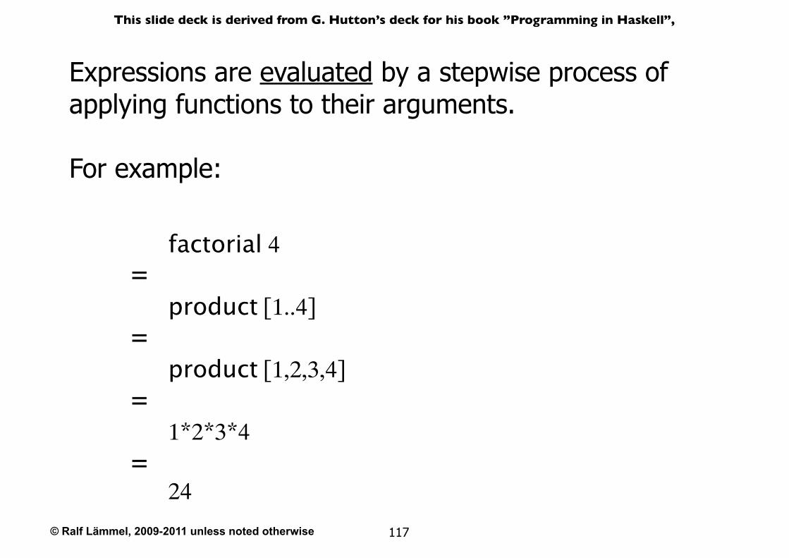
Expressions are evaluated by a stepwise process of applying functions to their arguments.
For example:
factorial 4
product [1..4]=
product [1,2,3,4]=
1*2*3*4=
24=
© Ralf Lämmel, 2009-2011 unless noted otherwise
This slide deck is derived from G. Hutton’s deck for his book ”Programming in Haskell”,
118
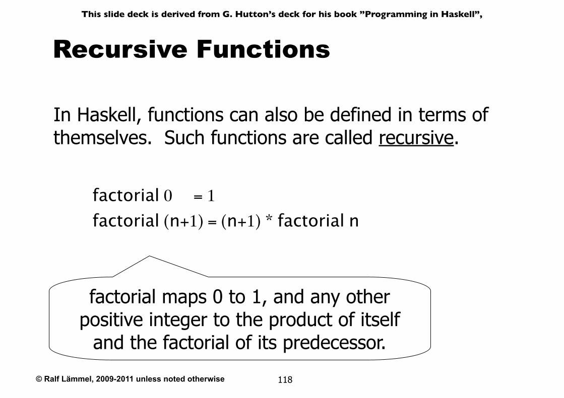
Recursive Functions
In Haskell, functions can also be defined in terms of themselves. Such functions are called recursive.
factorial 0 = 1
factorial (n+1) = (n+1) * factorial n
factorial maps 0 to 1, and any other positive integer to the product of itself
and the factorial of its predecessor.
© Ralf Lämmel, 2009-2011 unless noted otherwise
This slide deck is derived from G. Hutton’s deck for his book ”Programming in Haskell”,
119
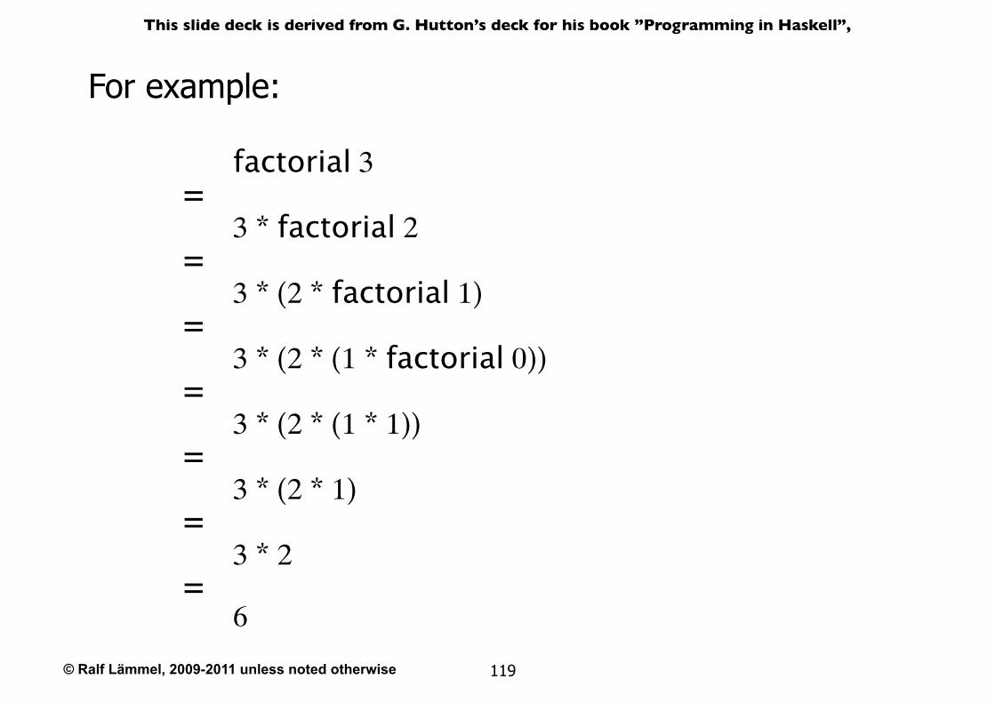
For example:
factorial 3
3 * factorial 2=
3 * (2 * factorial 1)=
3 * (2 * (1 * factorial 0))=
3 * (2 * (1 * 1))=
3 * (2 * 1)=
=6
3 * 2=
© Ralf Lämmel, 2009-2011 unless noted otherwise
This slide deck is derived from G. Hutton’s deck for his book ”Programming in Haskell”,
120
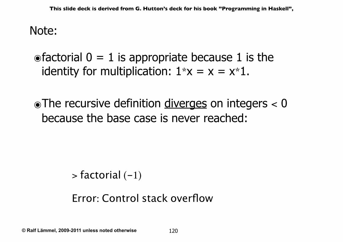
Note:
๏factorial 0 = 1 is appropriate because 1 is the identity for multiplication: 1*x = x = x*1.
๏The recursive definition diverges on integers < 0 because the base case is never reached:
> factorial (-1)
Error: Control stack overflow
© Ralf Lämmel, 2009-2011 unless noted otherwise
This slide deck is derived from G. Hutton’s deck for his book ”Programming in Haskell”,
121
Why is Recursion Useful?
๏Some functions, such as factorial, are simpler to define in terms of other functions.
๏As we shall see, however, many functions can naturally be defined in terms of themselves.
๏Properties of functions defined using recursion can be proved using the simple but powerful mathematical technique of induction.
© Ralf Lämmel, 2009-2011 unless noted otherwise
This slide deck is derived from G. Hutton’s deck for his book ”Programming in Haskell”,
122
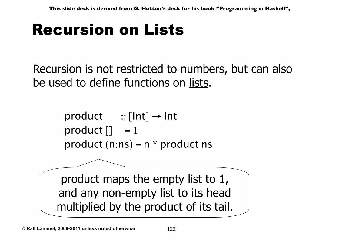
Recursion on Lists
Recursion is not restricted to numbers, but can also be used to define functions on lists.
product :: [Int] → Intproduct [] = 1product (n:ns) = n * product ns
product maps the empty list to 1, and any non-empty list to its head multiplied by the product of its tail.
© Ralf Lämmel, 2009-2011 unless noted otherwise
This slide deck is derived from G. Hutton’s deck for his book ”Programming in Haskell”,
123
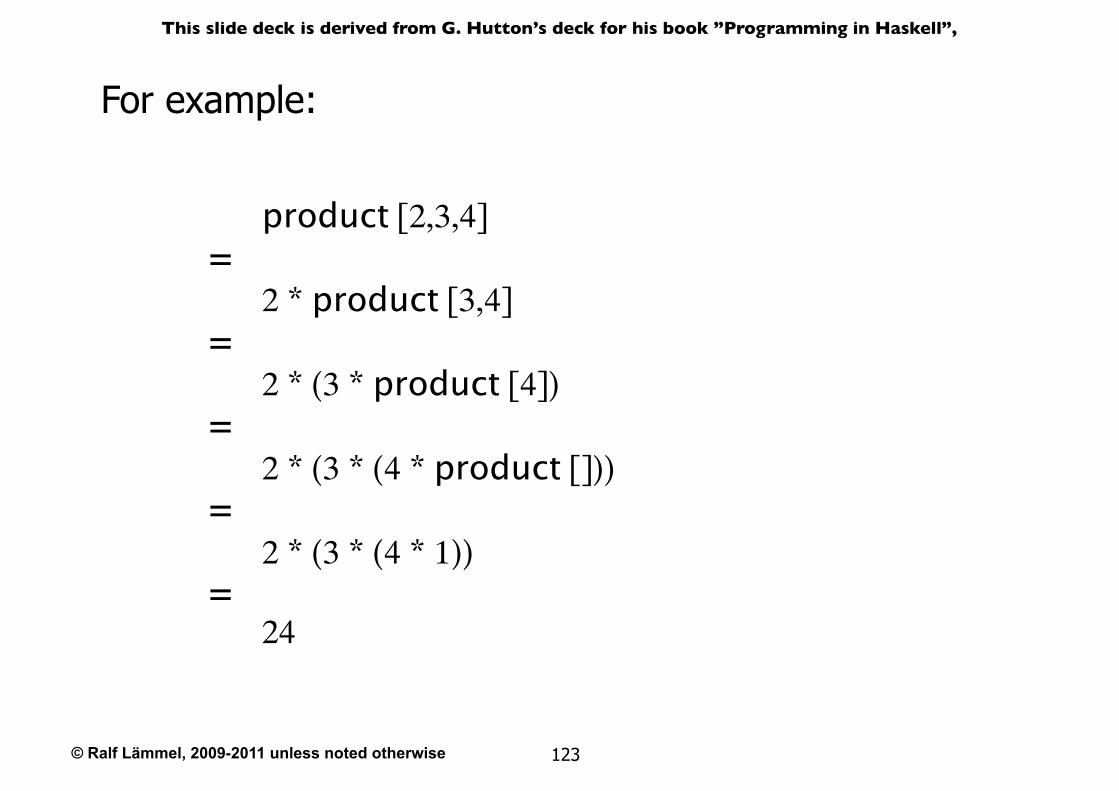
For example:
product [2,3,4]
2 * product [3,4]=
2 * (3 * product [4])=
2 * (3 * (4 * product []))=
2 * (3 * (4 * 1))=
24=
© Ralf Lämmel, 2009-2011 unless noted otherwise
This slide deck is derived from G. Hutton’s deck for his book ”Programming in Haskell”,
124
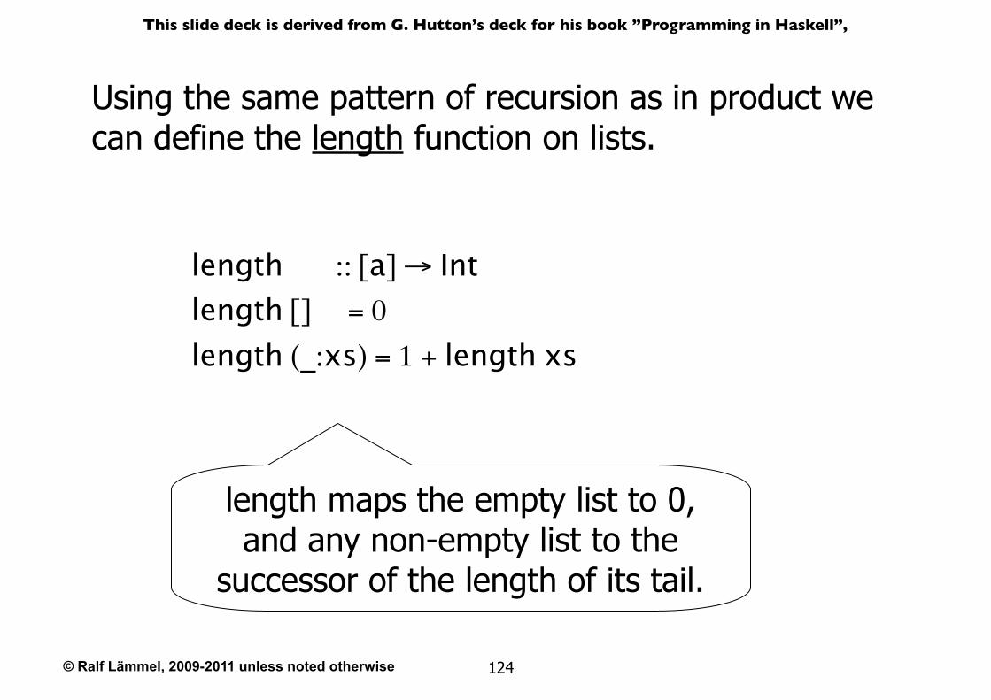
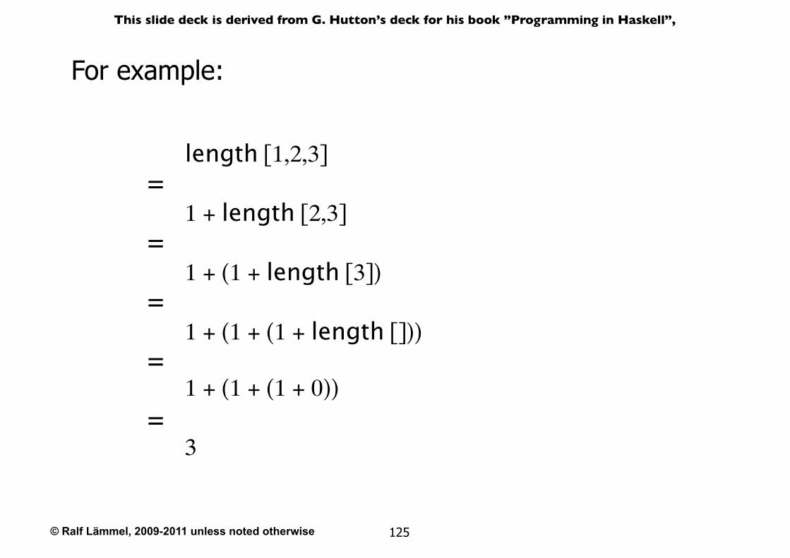
Using the same pattern of recursion as in product we can define the length function on lists.
length :: [a] → Intlength [] = 0
length (_:xs) = 1 + length xs
length maps the empty list to 0, and any non-empty list to the
successor of the length of its tail.
© Ralf Lämmel, 2009-2011 unless noted otherwise
This slide deck is derived from G. Hutton’s deck for his book ”Programming in Haskell”,
125
For example:
length [1,2,3]
1 + length [2,3]=
1 + (1 + length [3])=
1 + (1 + (1 + length []))=
1 + (1 + (1 + 0))=
3=
© Ralf Lämmel, 2009-2011 unless noted otherwise
This slide deck is derived from G. Hutton’s deck for his book ”Programming in Haskell”,
126
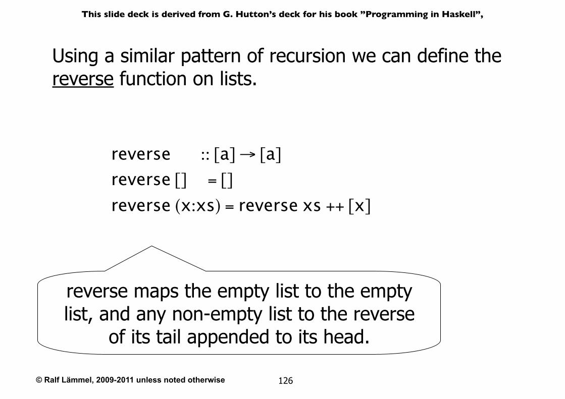
Using a similar pattern of recursion we can define the reverse function on lists.
reverse :: [a] → [a]
reverse [] = []
reverse (x:xs) = reverse xs ++ [x]
reverse maps the empty list to the empty list, and any non-empty list to the reverse
of its tail appended to its head.
© Ralf Lämmel, 2009-2011 unless noted otherwise
This slide deck is derived from G. Hutton’s deck for his book ”Programming in Haskell”,
127
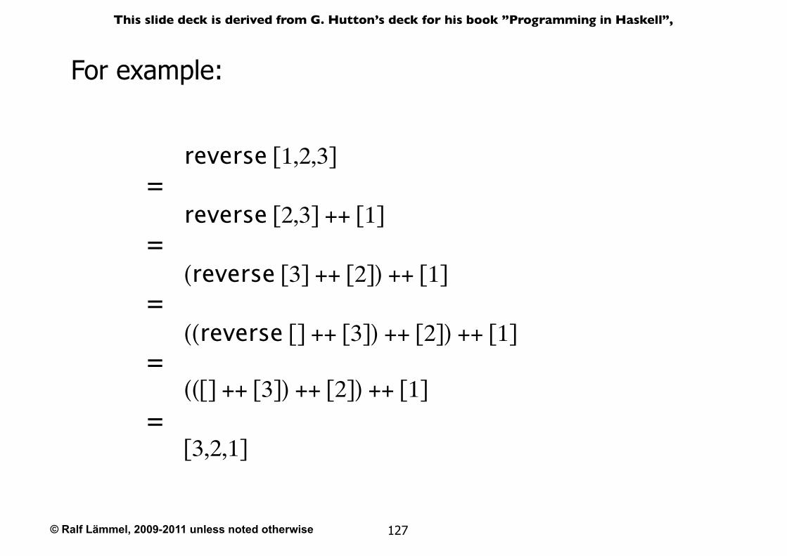
For example:
reverse [1,2,3]
reverse [2,3] ++ [1]=
(reverse [3] ++ [2]) ++ [1]=
((reverse [] ++ [3]) ++ [2]) ++ [1]=
(([] ++ [3]) ++ [2]) ++ [1]=
[3,2,1]=
© Ralf Lämmel, 2009-2011 unless noted otherwise
This slide deck is derived from G. Hutton’s deck for his book ”Programming in Haskell”,
128
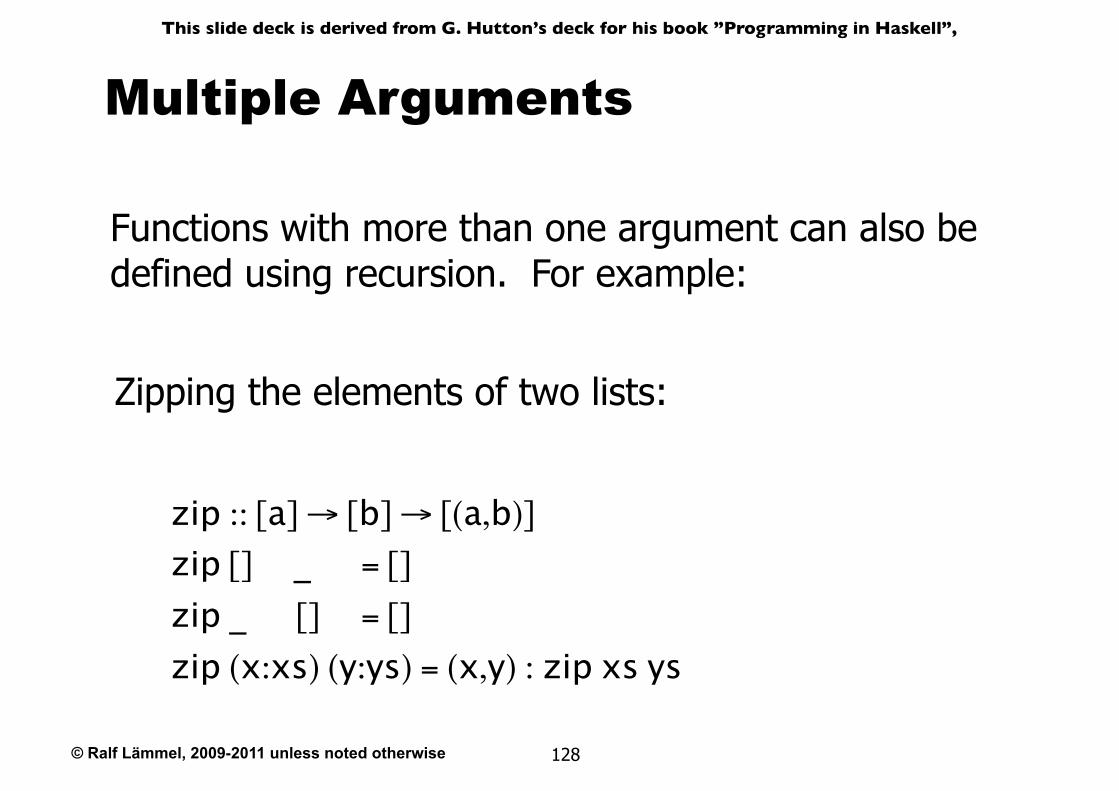
Multiple Arguments
Functions with more than one argument can also be defined using recursion. For example:
Zipping the elements of two lists:
zip :: [a] → [b] → [(a,b)]
zip [] _ = []
zip _ [] = []
zip (x:xs) (y:ys) = (x,y) : zip xs ys
© Ralf Lämmel, 2009-2011 unless noted otherwise
This slide deck is derived from G. Hutton’s deck for his book ”Programming in Haskell”,
129
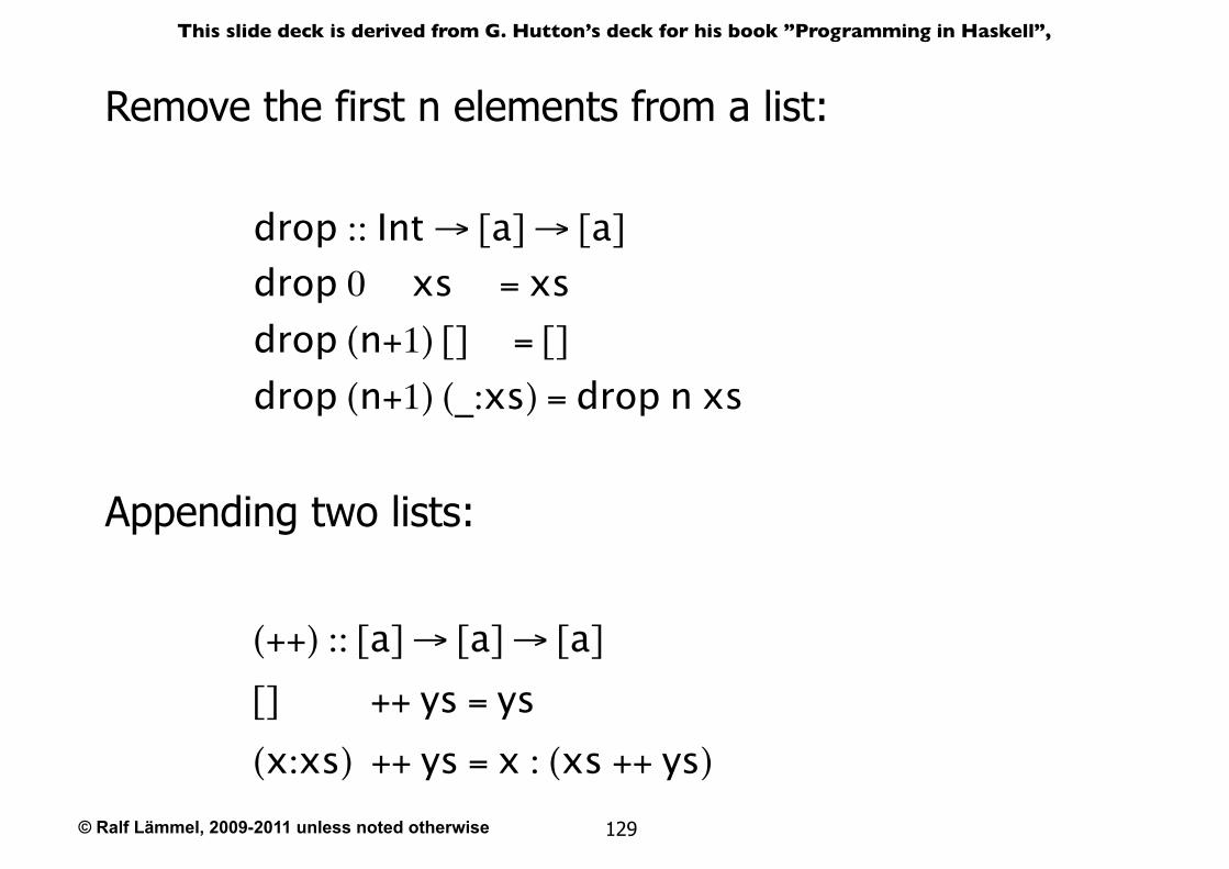
drop :: Int → [a] → [a]
drop 0 xs = xsdrop (n+1) [] = []
drop (n+1) (_:xs) = drop n xs
Remove the first n elements from a list:
(++) :: [a] → [a] → [a]
[] ++ ys = ys(x:xs) ++ ys = x : (xs ++ ys)
Appending two lists:
© Ralf Lämmel, 2009-2011 unless noted otherwise
This slide deck is derived from G. Hutton’s deck for his book ”Programming in Haskell”,
130
Quicksort
The quicksort algorithm for sorting a list of integers can be specified by the following two rules:
The empty list is already sorted;
Non-empty lists can be sorted by sorting the tail values ≤ the head, sorting the tail values > the head, and then appending the resulting lists on either side of the head value.
© Ralf Lämmel, 2009-2011 unless noted otherwise
This slide deck is derived from G. Hutton’s deck for his book ”Programming in Haskell”,
131
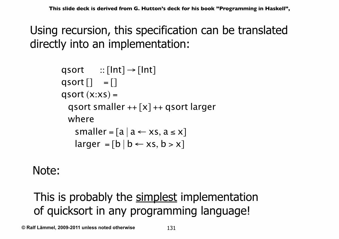
Using recursion, this specification can be translated directly into an implementation:
qsort :: [Int] → [Int]qsort [] = []qsort (x:xs) = qsort smaller ++ [x] ++ qsort larger where smaller = [a | a ← xs, a ≤ x] larger = [b | b ← xs, b > x]
This is probably the simplest implementation of quicksort in any programming language!
Note:
© Ralf Lämmel, 2009-2011 unless noted otherwise
This slide deck is derived from G. Hutton’s deck for his book ”Programming in Haskell”,
132
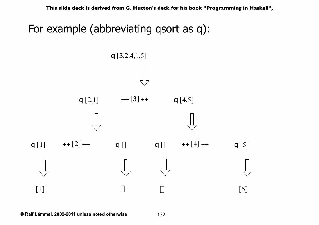
For example (abbreviating qsort as q):
q [3,2,4,1,5]
q [2,1] ++ [3] ++ q [4,5]
q [1] q []++ [2] ++ q [] q [5]++ [4] ++
[1] [] [] [5]
© Ralf Lämmel, 2009-2011 unless noted otherwise
This slide deck is derived from G. Hutton’s deck for his book ”Programming in Haskell”,
133
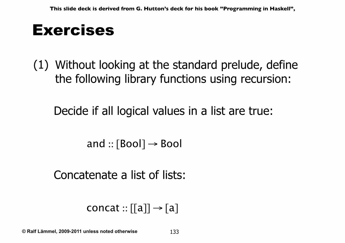
Exercises
(1) Without looking at the standard prelude, define the following library functions using recursion:
and :: [Bool] → Bool
Decide if all logical values in a list are true:
concat :: [[a]] → [a]
Concatenate a list of lists:
© Ralf Lämmel, 2009-2011 unless noted otherwise
This slide deck is derived from G. Hutton’s deck for his book ”Programming in Haskell”,
134
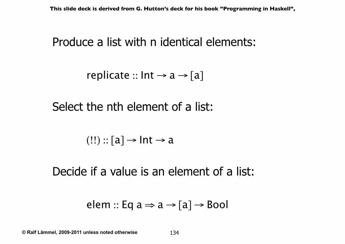
(!!) :: [a] → Int → a
Select the nth element of a list:
elem :: Eq a ⇒ a → [a] → Bool
Decide if a value is an element of a list:
replicate :: Int → a → [a]
Produce a list with n identical elements:
© Ralf Lämmel, 2009-2011 unless noted otherwise
This slide deck is derived from G. Hutton’s deck for his book ”Programming in Haskell”,
135
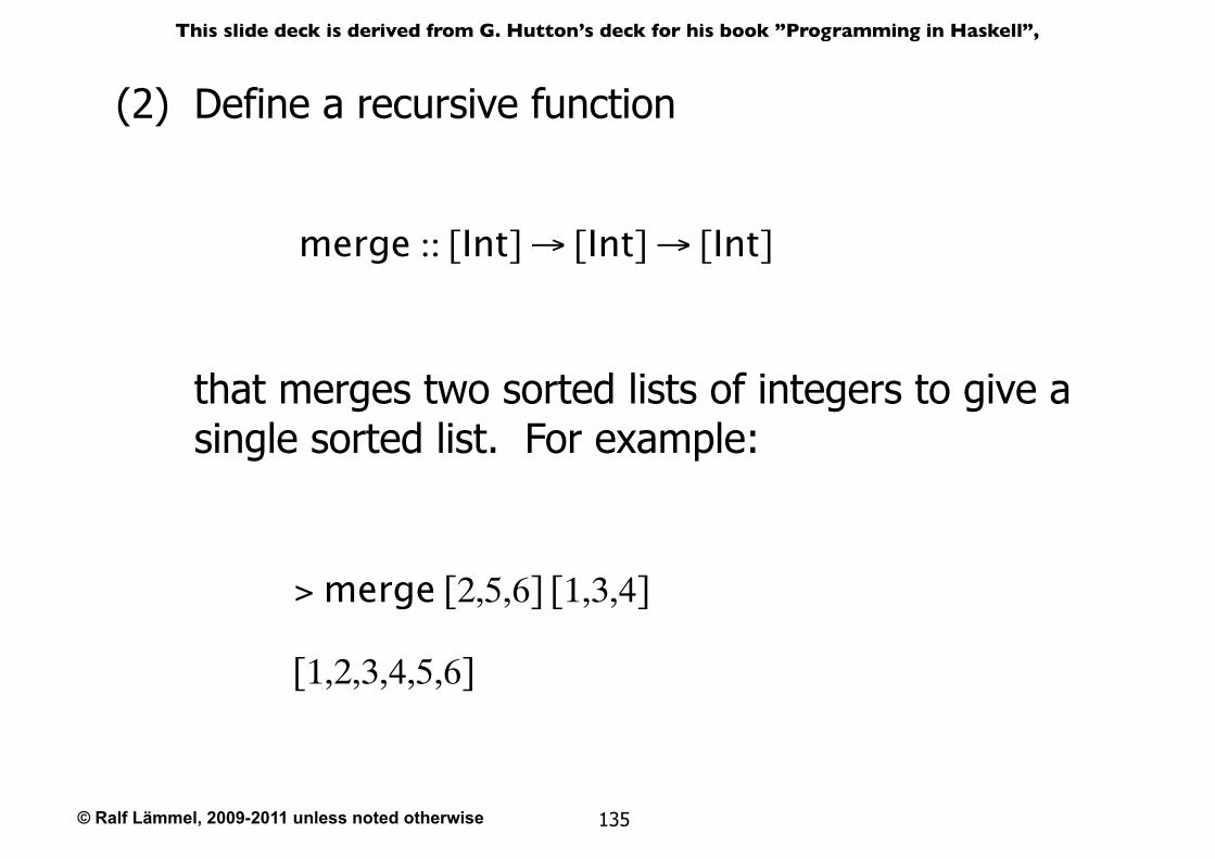
(2) Define a recursive function
merge :: [Int] → [Int] → [Int]
that merges two sorted lists of integers to give a single sorted list. For example:
> merge [2,5,6] [1,3,4]
[1,2,3,4,5,6]
© Ralf Lämmel, 2009-2011 unless noted otherwise
This slide deck is derived from G. Hutton’s deck for his book ”Programming in Haskell”,
136
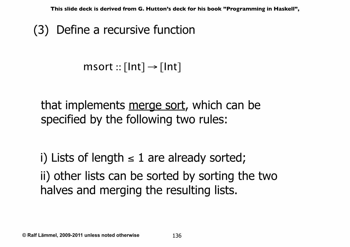
(3) Define a recursive function
i) Lists of length ≤ 1 are already sorted;ii) other lists can be sorted by sorting the two halves and merging the resulting lists.
msort :: [Int] → [Int]
that implements merge sort, which can be specified by the following two rules:
© Ralf Lämmel, 2009-2011 unless noted otherwise
This slide deck is derived from G. Hutton’s deck for his book ”Programming in Haskell”,
137
Higher-Order Functions
© Ralf Lämmel, 2009-2011 unless noted otherwise
This slide deck is derived from G. Hutton’s deck for his book ”Programming in Haskell”,
138
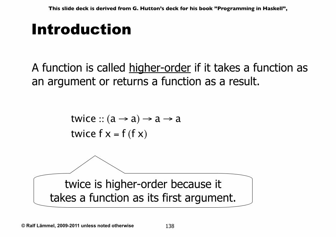
Introduction
A function is called higher-order if it takes a function as an argument or returns a function as a result.
twice :: (a → a) → a → atwice f x = f (f x)
twice is higher-order because ittakes a function as its first argument.
© Ralf Lämmel, 2009-2011 unless noted otherwise
This slide deck is derived from G. Hutton’s deck for his book ”Programming in Haskell”,
139
Why Are They Useful?
๏Common programming idioms can be encoded as functions within the language itself.
๏Domain specific languages can be defined as collections of higher-order functions.
๏Algebraic properties of higher-order functions can be used to reason about programs.
© Ralf Lämmel, 2009-2011 unless noted otherwise
This slide deck is derived from G. Hutton’s deck for his book ”Programming in Haskell”,
140
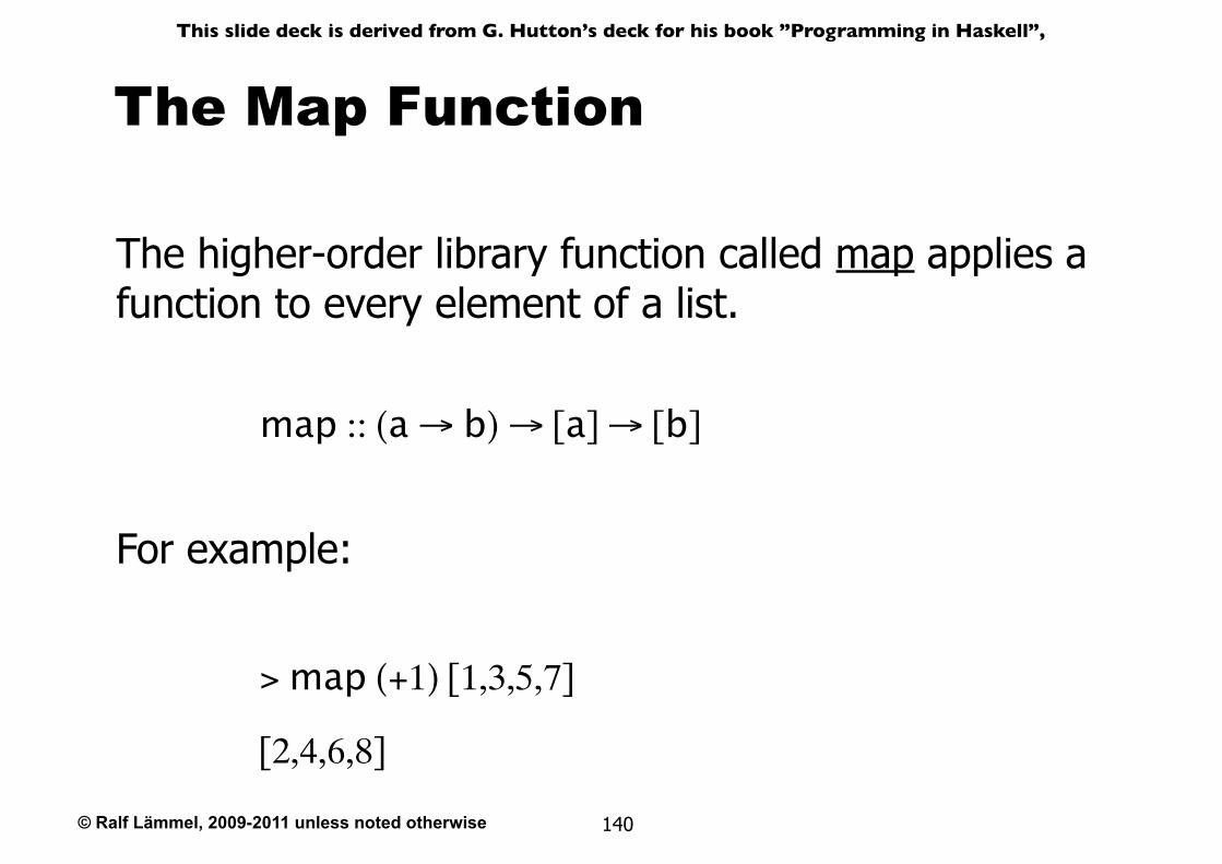
The Map Function
The higher-order library function called map applies a function to every element of a list.
map :: (a → b) → [a] → [b]
For example:
> map (+1) [1,3,5,7]
[2,4,6,8]
© Ralf Lämmel, 2009-2011 unless noted otherwise
This slide deck is derived from G. Hutton’s deck for his book ”Programming in Haskell”,
141
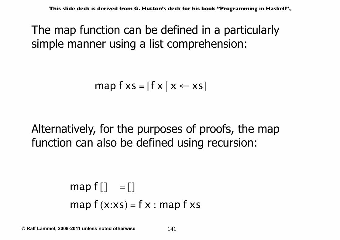
Alternatively, for the purposes of proofs, the map function can also be defined using recursion:
The map function can be defined in a particularly simple manner using a list comprehension:
map f xs = [f x | x ← xs]
map f [] = []
map f (x:xs) = f x : map f xs
© Ralf Lämmel, 2009-2011 unless noted otherwise
This slide deck is derived from G. Hutton’s deck for his book ”Programming in Haskell”,
142
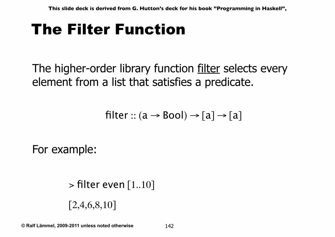
The Filter Function
The higher-order library function filter selects every element from a list that satisfies a predicate.
filter :: (a → Bool) → [a] → [a]
For example:
> filter even [1..10]
[2,4,6,8,10]
© Ralf Lämmel, 2009-2011 unless noted otherwise
This slide deck is derived from G. Hutton’s deck for his book ”Programming in Haskell”,
143
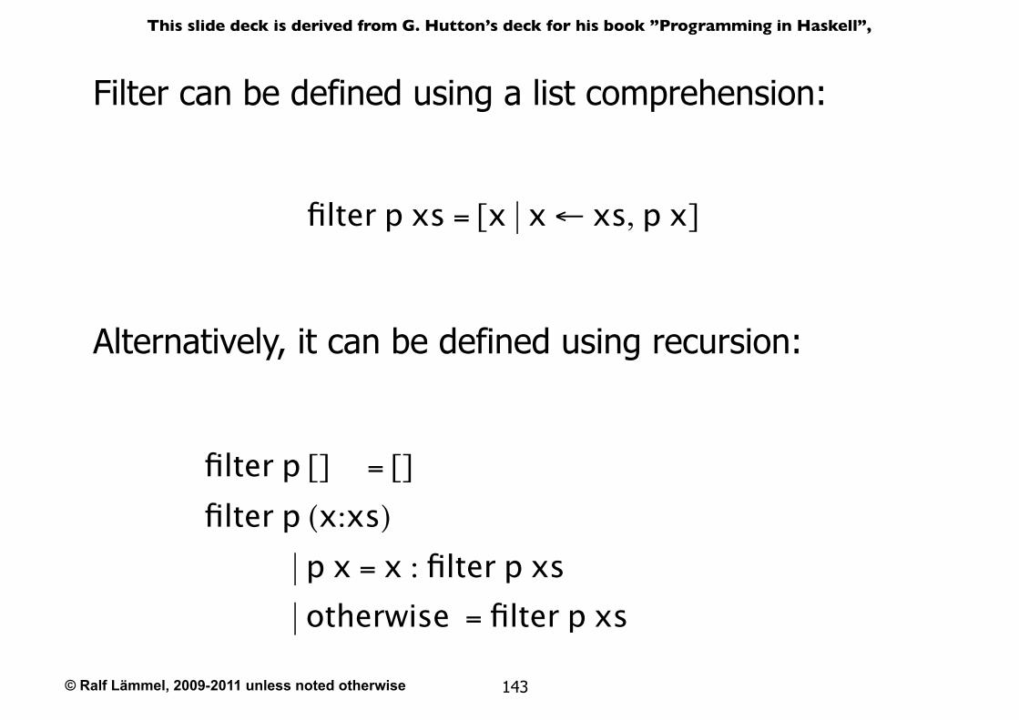
Alternatively, it can be defined using recursion:
Filter can be defined using a list comprehension:
filter p xs = [x | x ← xs, p x]
filter p [] = []
filter p (x:xs)
| p x = x : filter p xs | otherwise = filter p xs
© Ralf Lämmel, 2009-2011 unless noted otherwise
This slide deck is derived from G. Hutton’s deck for his book ”Programming in Haskell”,
144
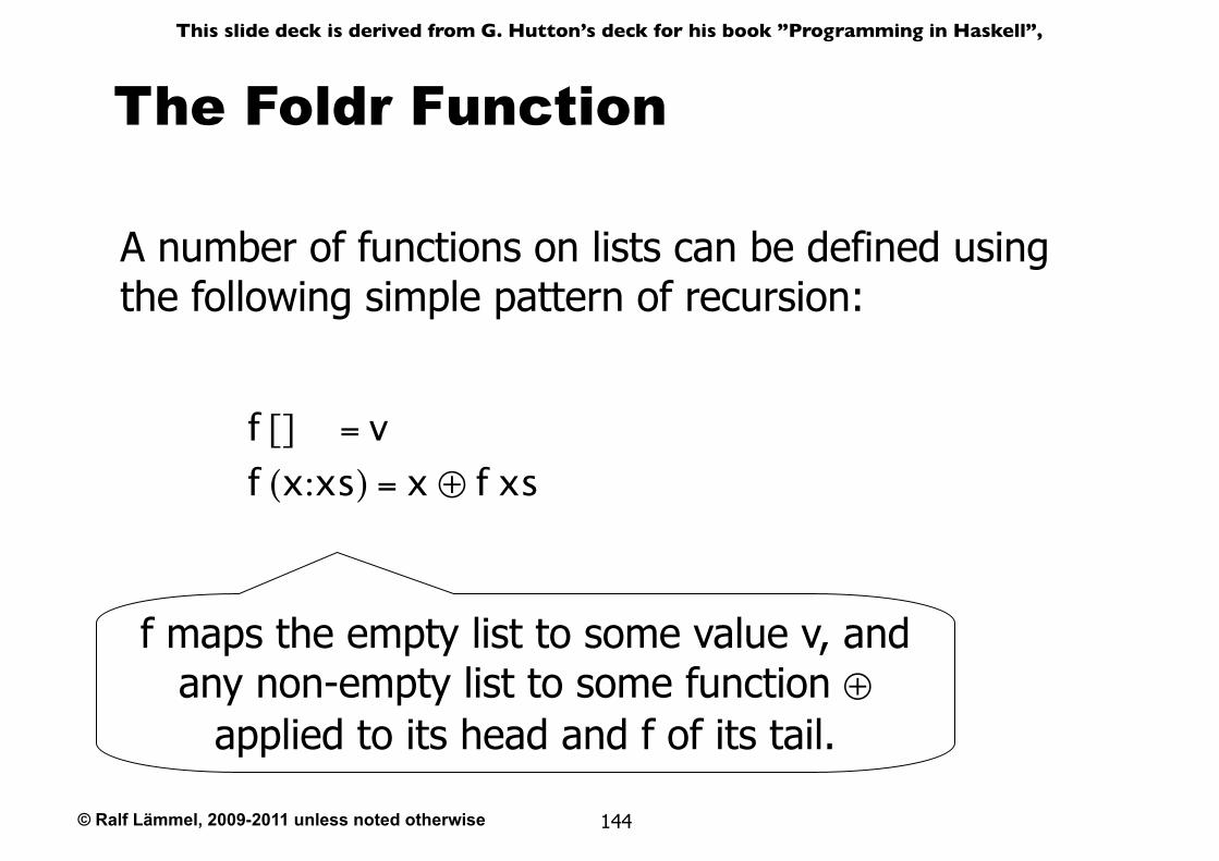
The Foldr Function
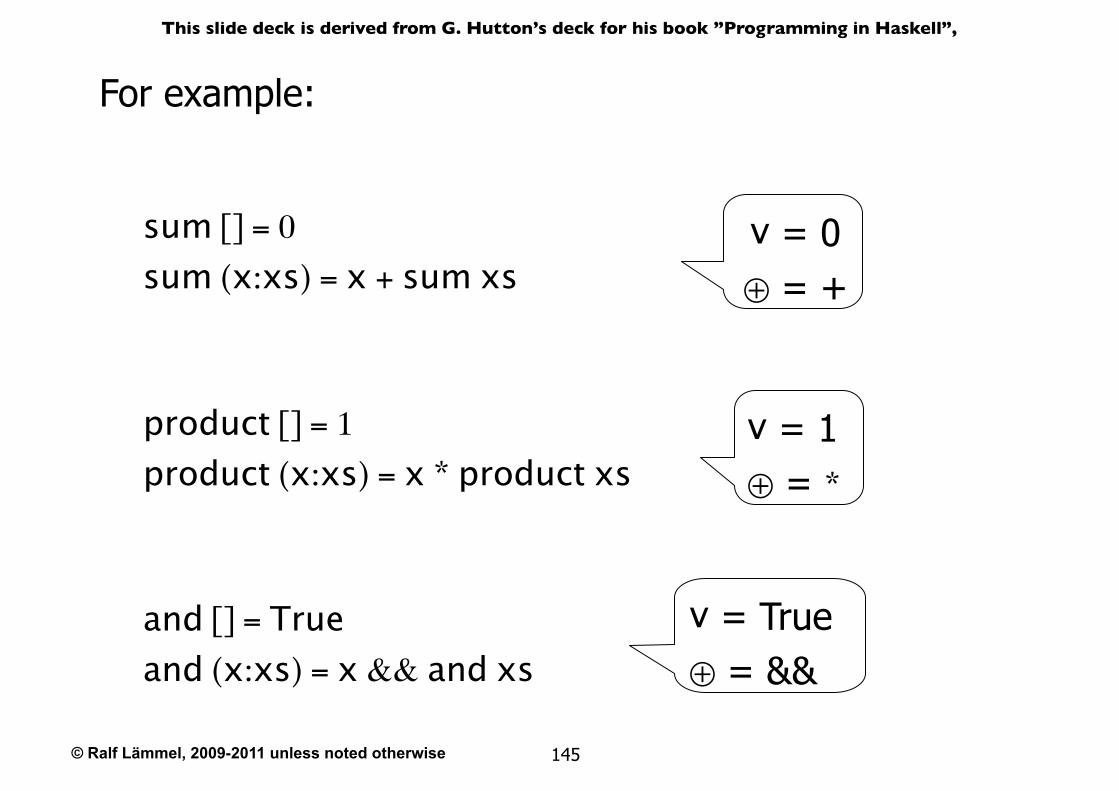
A number of functions on lists can be defined using the following simple pattern of recursion:
f [] = vf (x:xs) = x ⊕ f xs
f maps the empty list to some value v, and any non-empty list to some function ⊕
applied to its head and f of its tail.
© Ralf Lämmel, 2009-2011 unless noted otherwise
This slide deck is derived from G. Hutton’s deck for his book ”Programming in Haskell”,
145
For example:
sum [] = 0
sum (x:xs) = x + sum xs
and [] = Trueand (x:xs) = x && and xs
product [] = 1
product (x:xs) = x * product xs
v = 0⊕ = +
v = 1⊕ = *
v = True⊕ = &&
© Ralf Lämmel, 2009-2011 unless noted otherwise
This slide deck is derived from G. Hutton’s deck for his book ”Programming in Haskell”,
146
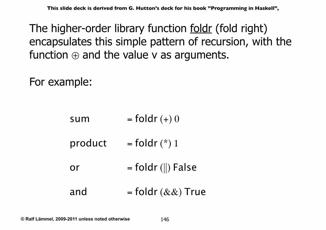
The higher-order library function foldr (fold right) encapsulates this simple pattern of recursion, with the function ⊕ and the value v as arguments.
For example:
sum = foldr (+) 0
product = foldr (*) 1
or = foldr (||) False
and = foldr (&&) True
© Ralf Lämmel, 2009-2011 unless noted otherwise
This slide deck is derived from G. Hutton’s deck for his book ”Programming in Haskell”,
147
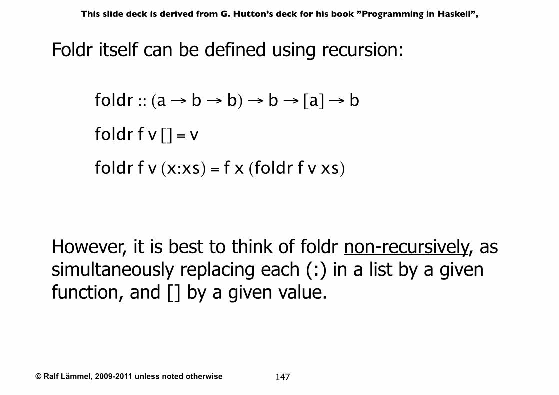
Foldr itself can be defined using recursion:
foldr :: (a → b → b) → b → [a] → b
foldr f v [] = v
foldr f v (x:xs) = f x (foldr f v xs)
However, it is best to think of foldr non-recursively, as simultaneously replacing each (:) in a list by a given function, and [] by a given value.
© Ralf Lämmel, 2009-2011 unless noted otherwise
This slide deck is derived from G. Hutton’s deck for his book ”Programming in Haskell”,
148
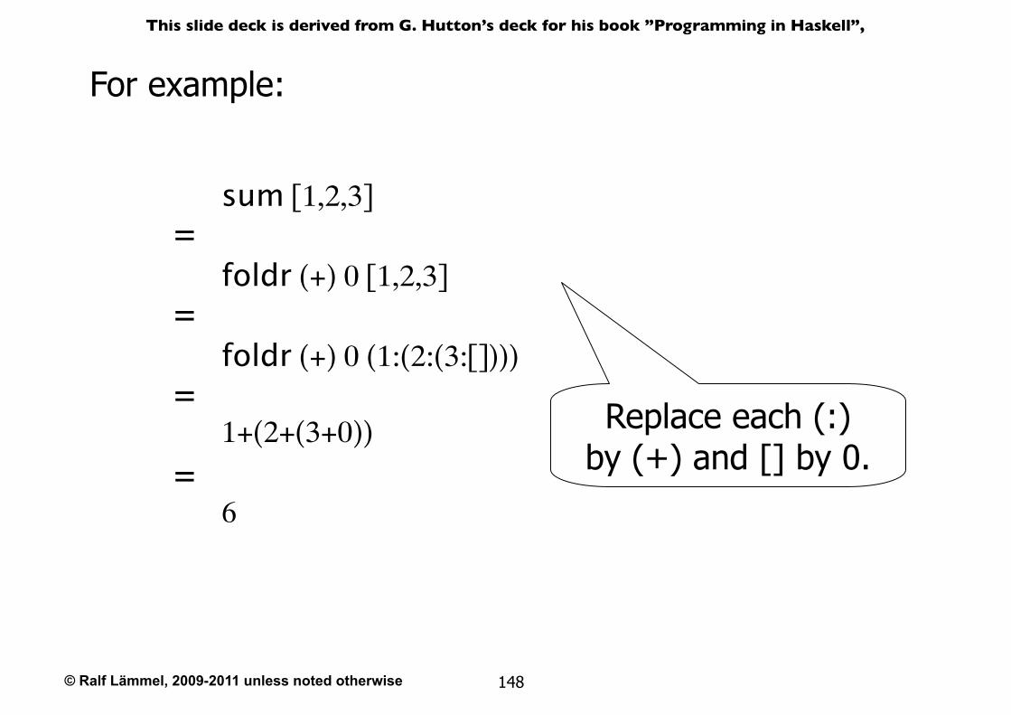
sum [1,2,3]
foldr (+) 0 [1,2,3]=
foldr (+) 0 (1:(2:(3:[])))=
1+(2+(3+0))=
6=
For example:
Replace each (:)by (+) and [] by 0.
© Ralf Lämmel, 2009-2011 unless noted otherwise
This slide deck is derived from G. Hutton’s deck for his book ”Programming in Haskell”,
149
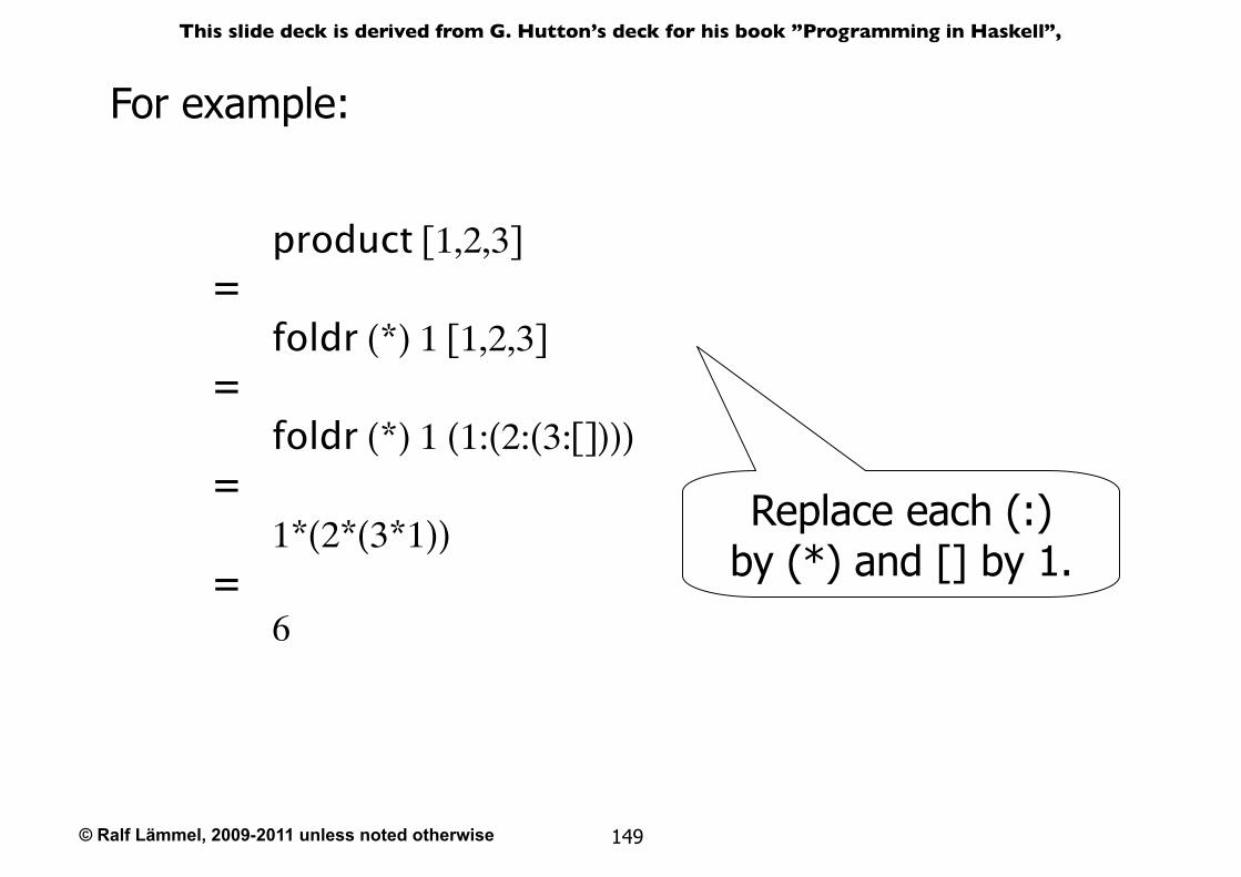
product [1,2,3]
foldr (*) 1 [1,2,3]=
foldr (*) 1 (1:(2:(3:[])))=
1*(2*(3*1))=
6=
For example:
Replace each (:)by (*) and [] by 1.
© Ralf Lämmel, 2009-2011 unless noted otherwise
This slide deck is derived from G. Hutton’s deck for his book ”Programming in Haskell”,
150
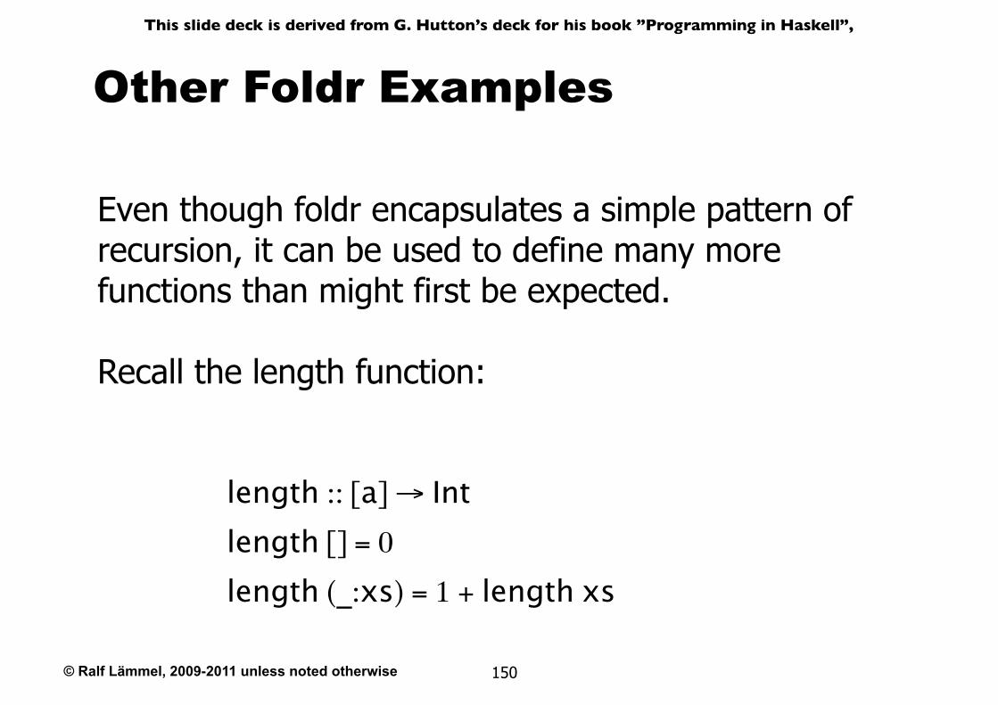
Other Foldr Examples
Even though foldr encapsulates a simple pattern of recursion, it can be used to define many more functions than might first be expected.
Recall the length function:
length :: [a] → Intlength [] = 0
length (_:xs) = 1 + length xs
© Ralf Lämmel, 2009-2011 unless noted otherwise
This slide deck is derived from G. Hutton’s deck for his book ”Programming in Haskell”,
151
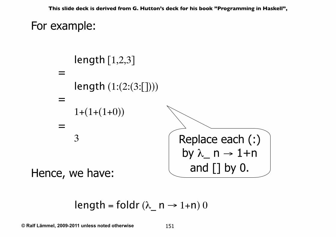
length [1,2,3]
length (1:(2:(3:[])))=
1+(1+(1+0))=
3=
Hence, we have:
length = foldr (λ_ n → 1+n) 0
Replace each (:) by λ_ n → 1+n
and [] by 0.
For example:
© Ralf Lämmel, 2009-2011 unless noted otherwise
This slide deck is derived from G. Hutton’s deck for his book ”Programming in Haskell”,
152
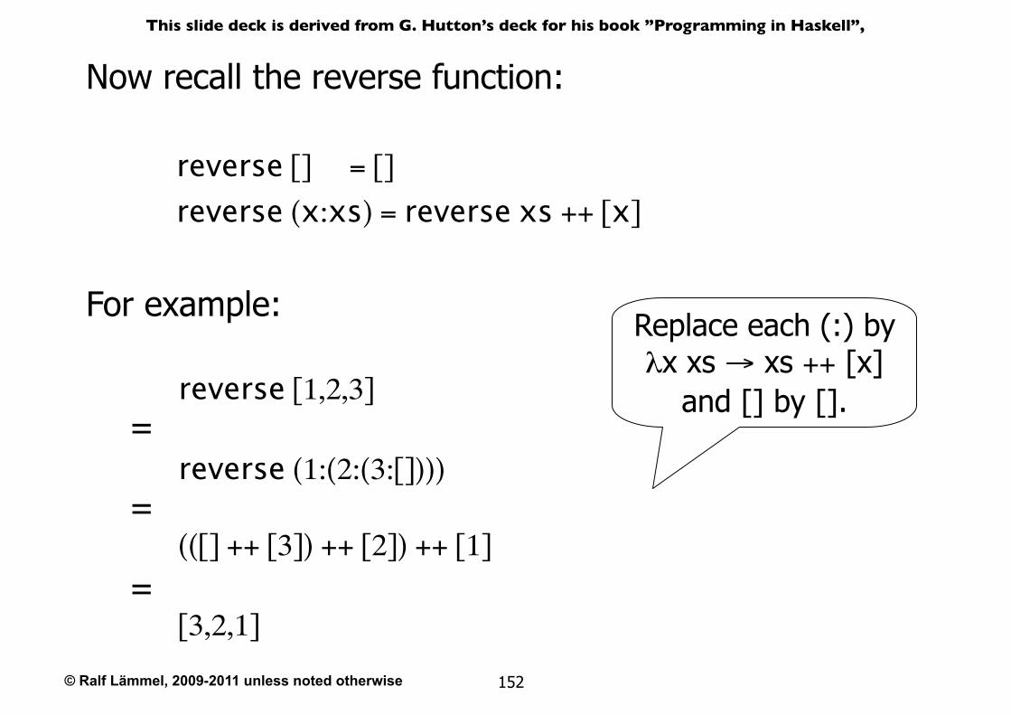
Now recall the reverse function:
reverse [] = []
reverse (x:xs) = reverse xs ++ [x]
reverse [1,2,3]
reverse (1:(2:(3:[])))=
(([] ++ [3]) ++ [2]) ++ [1]=
[3,2,1]=
For example:Replace each (:) by λx xs → xs ++ [x]
and [] by [].
© Ralf Lämmel, 2009-2011 unless noted otherwise
This slide deck is derived from G. Hutton’s deck for his book ”Programming in Haskell”,
153
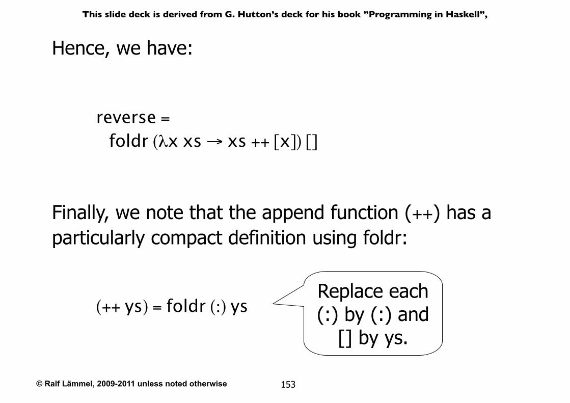
Hence, we have:
reverse = foldr (λx xs → xs ++ [x]) []
Finally, we note that the append function (++) has a particularly compact definition using foldr:
(++ ys) = foldr (:) ysReplace each (:) by (:) and
[] by ys.
© Ralf Lämmel, 2009-2011 unless noted otherwise
This slide deck is derived from G. Hutton’s deck for his book ”Programming in Haskell”,
154
Why Is Foldr Useful?
๏Some recursive functions on lists, such as sum, are simpler to define using foldr.
๏Properties of functions defined using foldr can be proved using algebraic properties of foldr, such as fusion and the banana split rule.
๏Advanced program optimisations can be simpler if foldr is used in place of explicit recursion.
© Ralf Lämmel, 2009-2011 unless noted otherwise
This slide deck is derived from G. Hutton’s deck for his book ”Programming in Haskell”,
155
Other Library Functions
The library function (.) returns the composition of two functions as a single function.
(.) :: (b → c) → (a → b) → (a → c)
f . g = λx → f (g x)
For example:
odd :: Int → Boolodd = not . even
© Ralf Lämmel, 2009-2011 unless noted otherwise
This slide deck is derived from G. Hutton’s deck for his book ”Programming in Haskell”,
156
The library function all decides if every element of a list satisfies a given predicate.
all :: (a → Bool) → [a] → Boolall p xs = and [p x | x ← xs]
For example:
> all even [2,4,6,8,10]
True
© Ralf Lämmel, 2009-2011 unless noted otherwise
This slide deck is derived from G. Hutton’s deck for his book ”Programming in Haskell”,
157
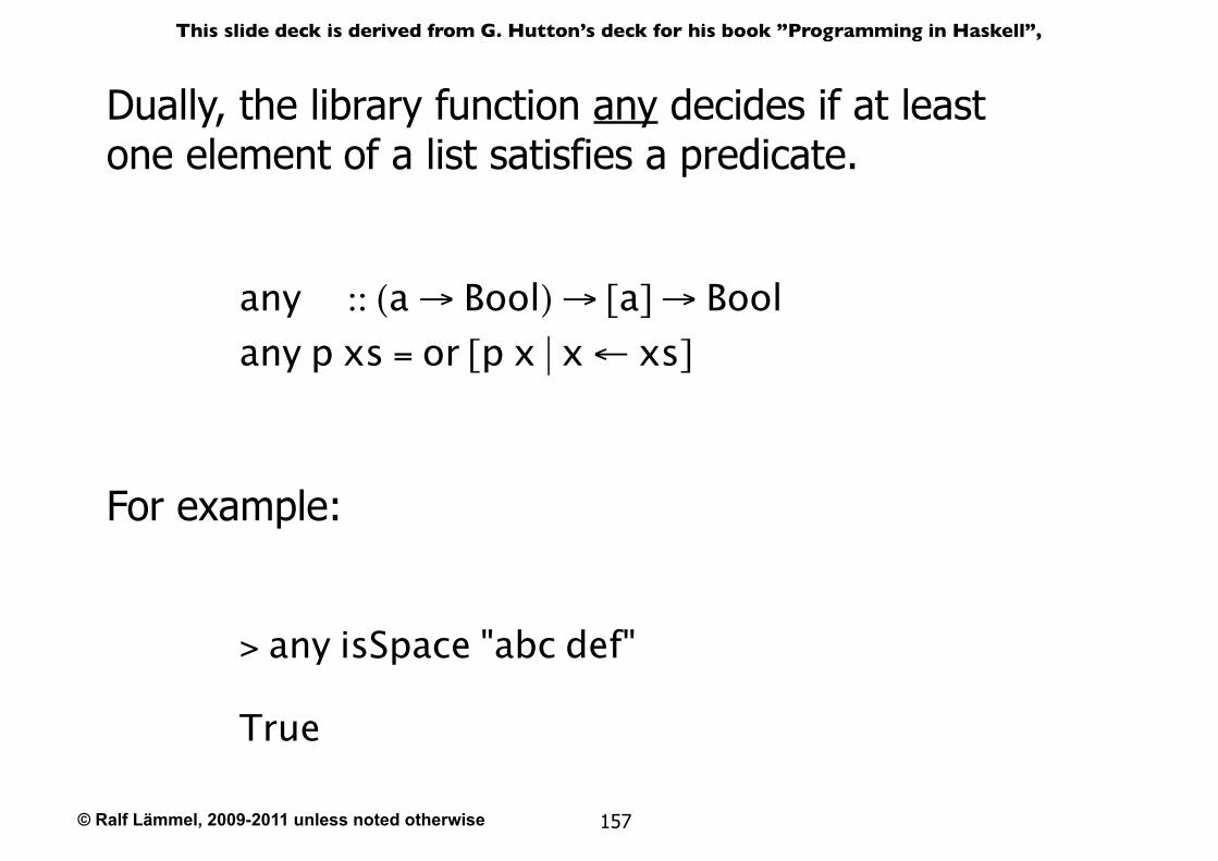
Dually, the library function any decides if at leastone element of a list satisfies a predicate.
any :: (a → Bool) → [a] → Boolany p xs = or [p x | x ← xs]
For example:
> any isSpace "abc def"
True
© Ralf Lämmel, 2009-2011 unless noted otherwise
This slide deck is derived from G. Hutton’s deck for his book ”Programming in Haskell”,
158
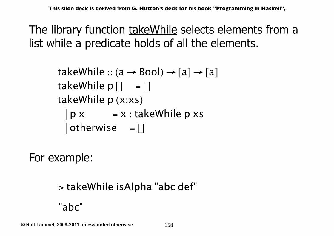
The library function takeWhile selects elements from a list while a predicate holds of all the elements.
takeWhile :: (a → Bool) → [a] → [a]takeWhile p [] = []takeWhile p (x:xs)
| p x = x : takeWhile p xs | otherwise = []
For example:
> takeWhile isAlpha "abc def"
"abc"
© Ralf Lämmel, 2009-2011 unless noted otherwise
This slide deck is derived from G. Hutton’s deck for his book ”Programming in Haskell”,
159
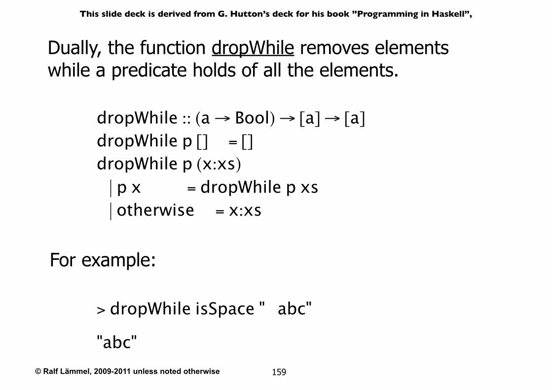
Dually, the function dropWhile removes elements while a predicate holds of all the elements.
dropWhile :: (a → Bool) → [a] → [a]dropWhile p [] = []dropWhile p (x:xs)
| p x = dropWhile p xs | otherwise = x:xs
For example:
> dropWhile isSpace " abc"
"abc"
© Ralf Lämmel, 2009-2011 unless noted otherwise
This slide deck is derived from G. Hutton’s deck for his book ”Programming in Haskell”,
160
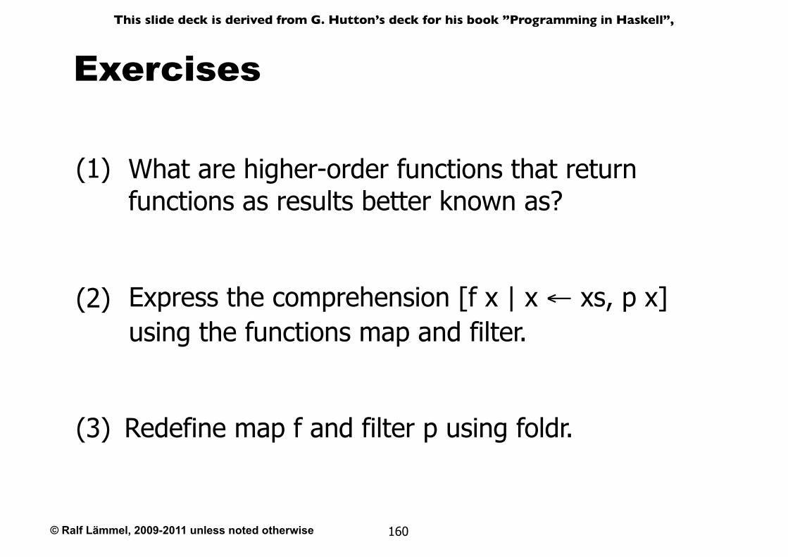
Exercises
(3) Redefine map f and filter p using foldr.
(2) Express the comprehension [f x | x ← xs, p x] using the functions map and filter.
(1) What are higher-order functions that return functions as results better known as?
© Ralf Lämmel, 2009-2011 unless noted otherwise
This slide deck is derived from G. Hutton’s deck for his book ”Programming in Haskell”,
161
Type Declarations
© Ralf Lämmel, 2009-2011 unless noted otherwise
This slide deck is derived from G. Hutton’s deck for his book ”Programming in Haskell”,
162
Type Declarations
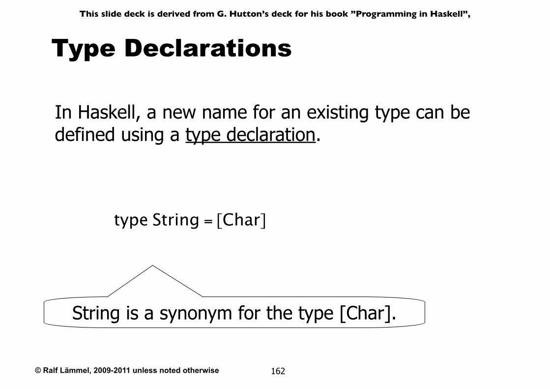
In Haskell, a new name for an existing type can be defined using a type declaration.
type String = [Char]
String is a synonym for the type [Char].
© Ralf Lämmel, 2009-2011 unless noted otherwise
This slide deck is derived from G. Hutton’s deck for his book ”Programming in Haskell”,
163
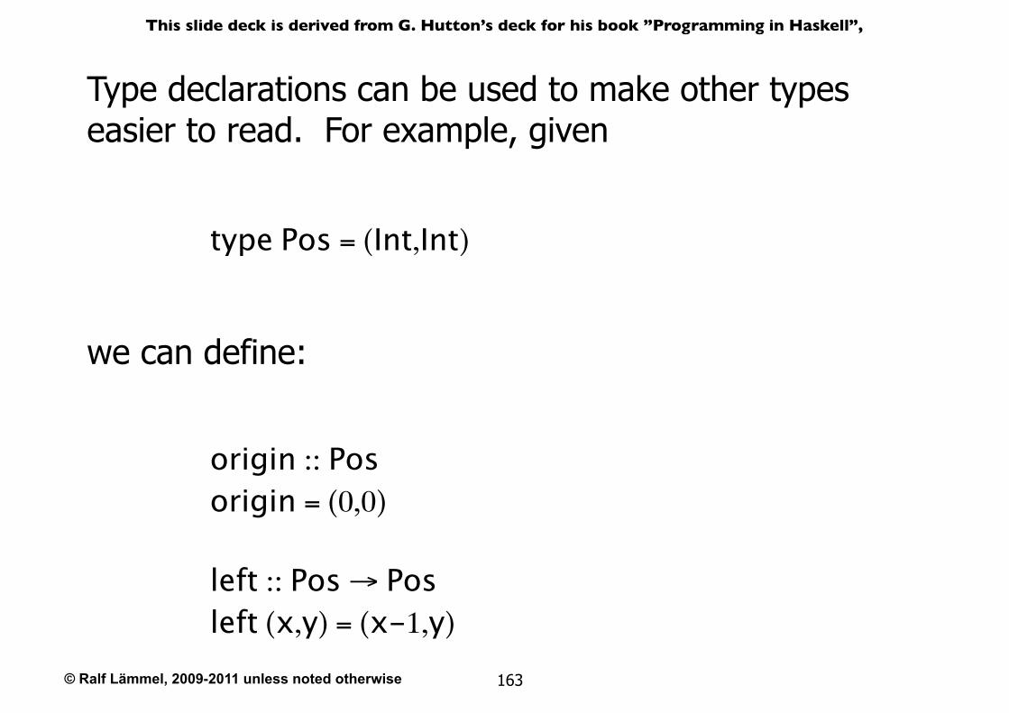
Type declarations can be used to make other types easier to read. For example, given
origin :: Posorigin = (0,0)
left :: Pos → Posleft (x,y) = (x-1,y)
type Pos = (Int,Int)
we can define:
© Ralf Lämmel, 2009-2011 unless noted otherwise
This slide deck is derived from G. Hutton’s deck for his book ”Programming in Haskell”,
164
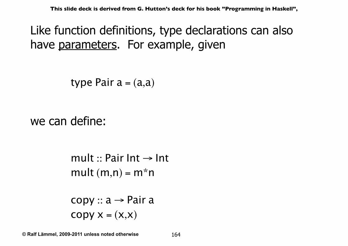
Like function definitions, type declarations can also have parameters. For example, given
type Pair a = (a,a)
we can define:
mult :: Pair Int → Intmult (m,n) = m*n
copy :: a → Pair acopy x = (x,x)
© Ralf Lämmel, 2009-2011 unless noted otherwise
This slide deck is derived from G. Hutton’s deck for his book ”Programming in Haskell”,
165
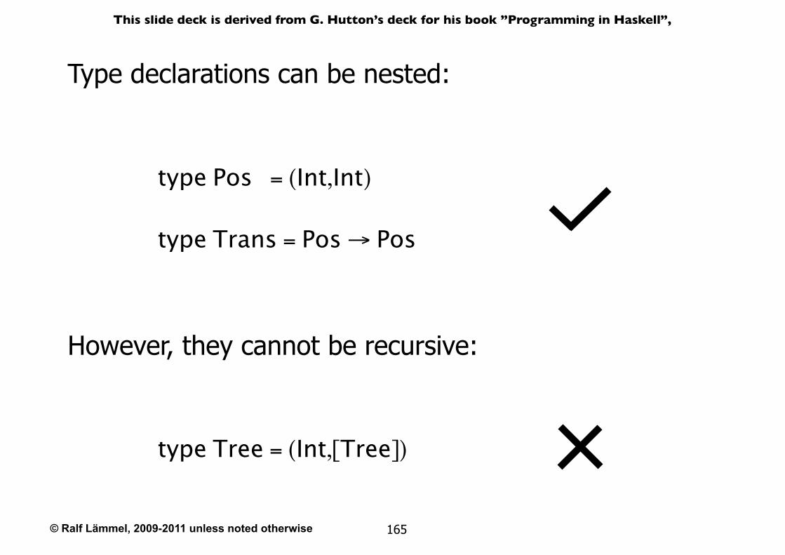
Type declarations can be nested:
type Pos = (Int,Int)
type Trans = Pos → Pos
However, they cannot be recursive:
type Tree = (Int,[Tree])
© Ralf Lämmel, 2009-2011 unless noted otherwise
This slide deck is derived from G. Hutton’s deck for his book ”Programming in Haskell”,
166
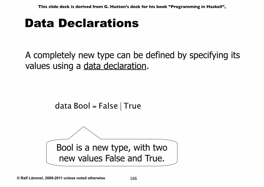
Data Declarations
A completely new type can be defined by specifying its values using a data declaration.
data Bool = False | True
Bool is a new type, with two new values False and True.
© Ralf Lämmel, 2009-2011 unless noted otherwise
This slide deck is derived from G. Hutton’s deck for his book ”Programming in Haskell”,
167
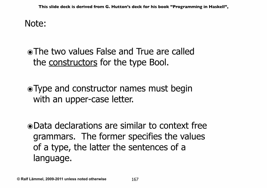
Note:
๏The two values False and True are called the constructors for the type Bool.
๏Type and constructor names must begin with an upper-case letter.
๏Data declarations are similar to context free grammars. The former specifies the values of a type, the latter the sentences of a language.
© Ralf Lämmel, 2009-2011 unless noted otherwise
This slide deck is derived from G. Hutton’s deck for his book ”Programming in Haskell”,
168
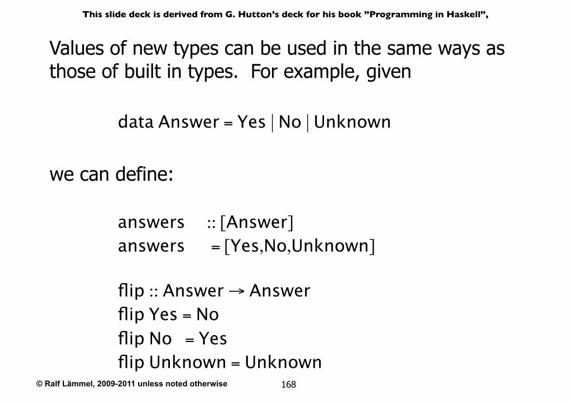
answers :: [Answer]answers = [Yes,No,Unknown]
flip :: Answer → Answerflip Yes = Noflip No = Yesflip Unknown = Unknown
data Answer = Yes | No | Unknown
we can define:
Values of new types can be used in the same ways as those of built in types. For example, given
© Ralf Lämmel, 2009-2011 unless noted otherwise
This slide deck is derived from G. Hutton’s deck for his book ”Programming in Haskell”,
169
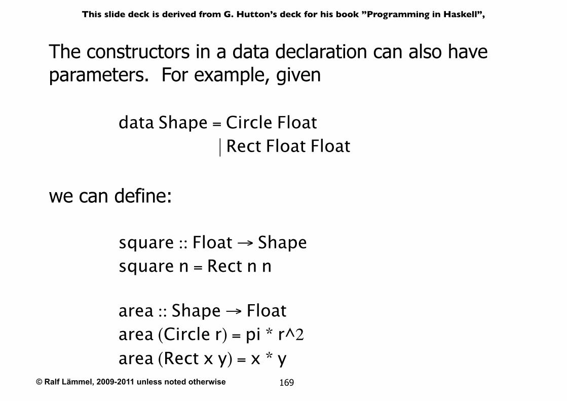
The constructors in a data declaration can also have parameters. For example, given
data Shape = Circle Float | Rect Float Float
square :: Float → Shapesquare n = Rect n n
area :: Shape → Floatarea (Circle r) = pi * r^2
area (Rect x y) = x * y
we can define:
© Ralf Lämmel, 2009-2011 unless noted otherwise
This slide deck is derived from G. Hutton’s deck for his book ”Programming in Haskell”,
170
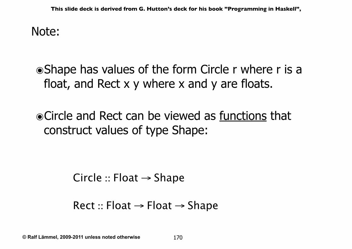
Note:
๏Shape has values of the form Circle r where r is a float, and Rect x y where x and y are floats.
๏Circle and Rect can be viewed as functions that construct values of type Shape:
Circle :: Float → Shape
Rect :: Float → Float → Shape
© Ralf Lämmel, 2009-2011 unless noted otherwise
This slide deck is derived from G. Hutton’s deck for his book ”Programming in Haskell”,
171
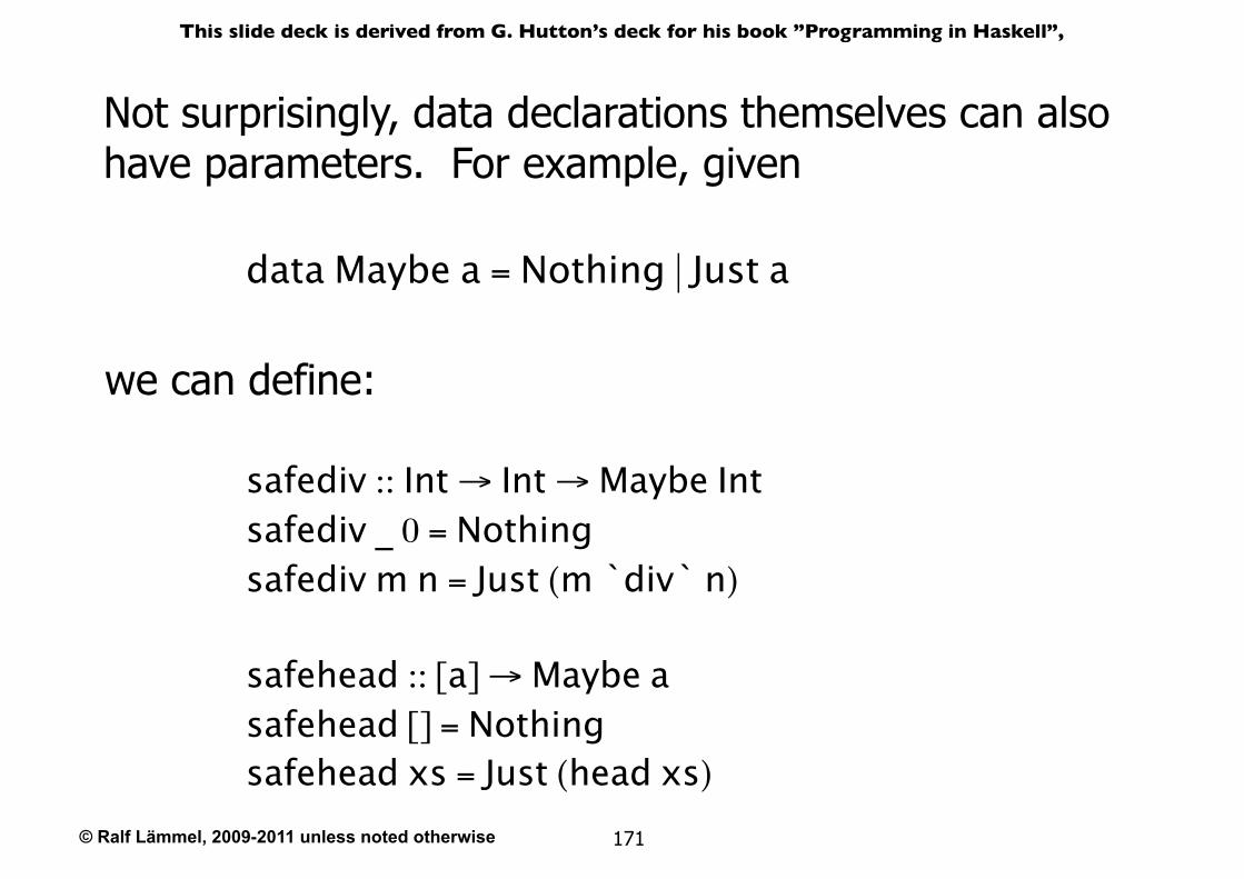
Not surprisingly, data declarations themselves can also have parameters. For example, given
data Maybe a = Nothing | Just a
safediv :: Int → Int → Maybe Intsafediv _ 0 = Nothingsafediv m n = Just (m `div` n)
safehead :: [a] → Maybe asafehead [] = Nothingsafehead xs = Just (head xs)
we can define:
© Ralf Lämmel, 2009-2011 unless noted otherwise
This slide deck is derived from G. Hutton’s deck for his book ”Programming in Haskell”,
172
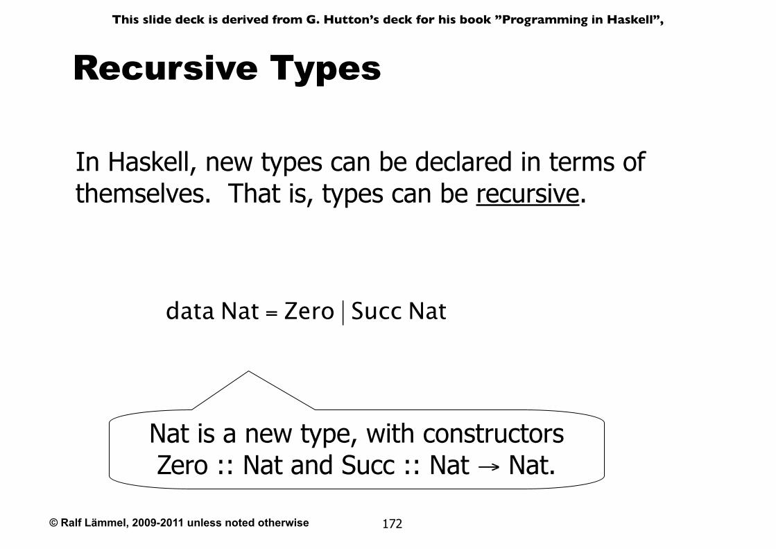
Recursive Types
In Haskell, new types can be declared in terms of themselves. That is, types can be recursive.
data Nat = Zero | Succ Nat
Nat is a new type, with constructors Zero :: Nat and Succ :: Nat → Nat.
© Ralf Lämmel, 2009-2011 unless noted otherwise
This slide deck is derived from G. Hutton’s deck for his book ”Programming in Haskell”,
173
Note:
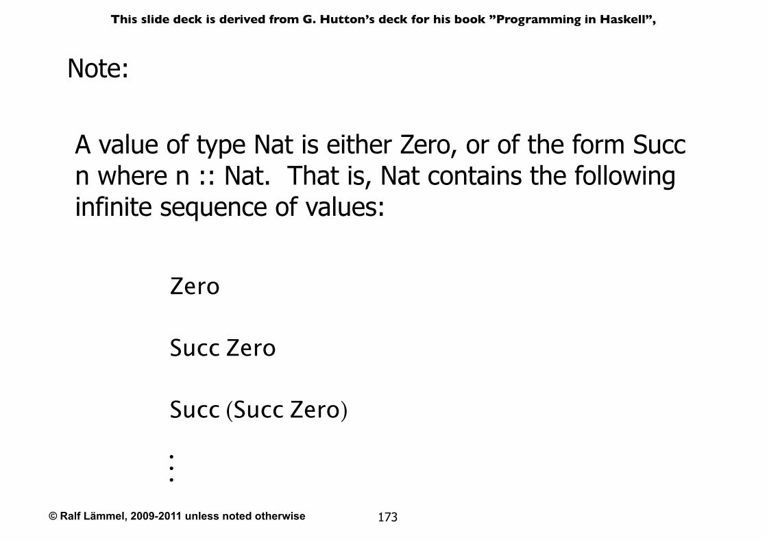
A value of type Nat is either Zero, or of the form Succ n where n :: Nat. That is, Nat contains the following infinite sequence of values:
Zero
Succ Zero
Succ (Succ Zero)
•••
© Ralf Lämmel, 2009-2011 unless noted otherwise
This slide deck is derived from G. Hutton’s deck for his book ”Programming in Haskell”,
174
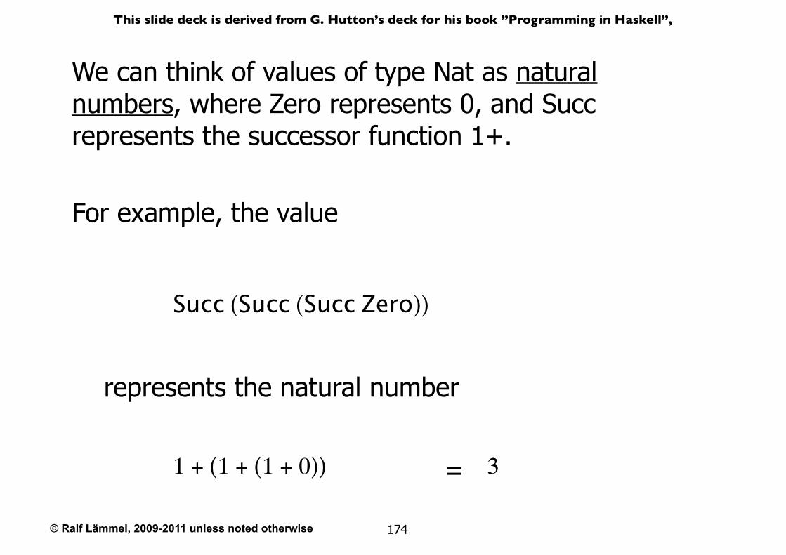
We can think of values of type Nat as natural numbers, where Zero represents 0, and Succ represents the successor function 1+.
For example, the value
Succ (Succ (Succ Zero))
represents the natural number
1 + (1 + (1 + 0)) 3=
© Ralf Lämmel, 2009-2011 unless noted otherwise
This slide deck is derived from G. Hutton’s deck for his book ”Programming in Haskell”,
175
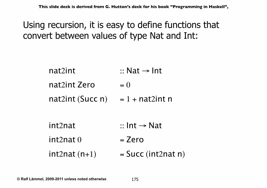
Using recursion, it is easy to define functions that convert between values of type Nat and Int:
nat2int :: Nat → Intnat2int Zero = 0
nat2int (Succ n) = 1 + nat2int n
int2nat :: Int → Natint2nat 0 = Zeroint2nat (n+1) = Succ (int2nat n)
© Ralf Lämmel, 2009-2011 unless noted otherwise
This slide deck is derived from G. Hutton’s deck for his book ”Programming in Haskell”,
176
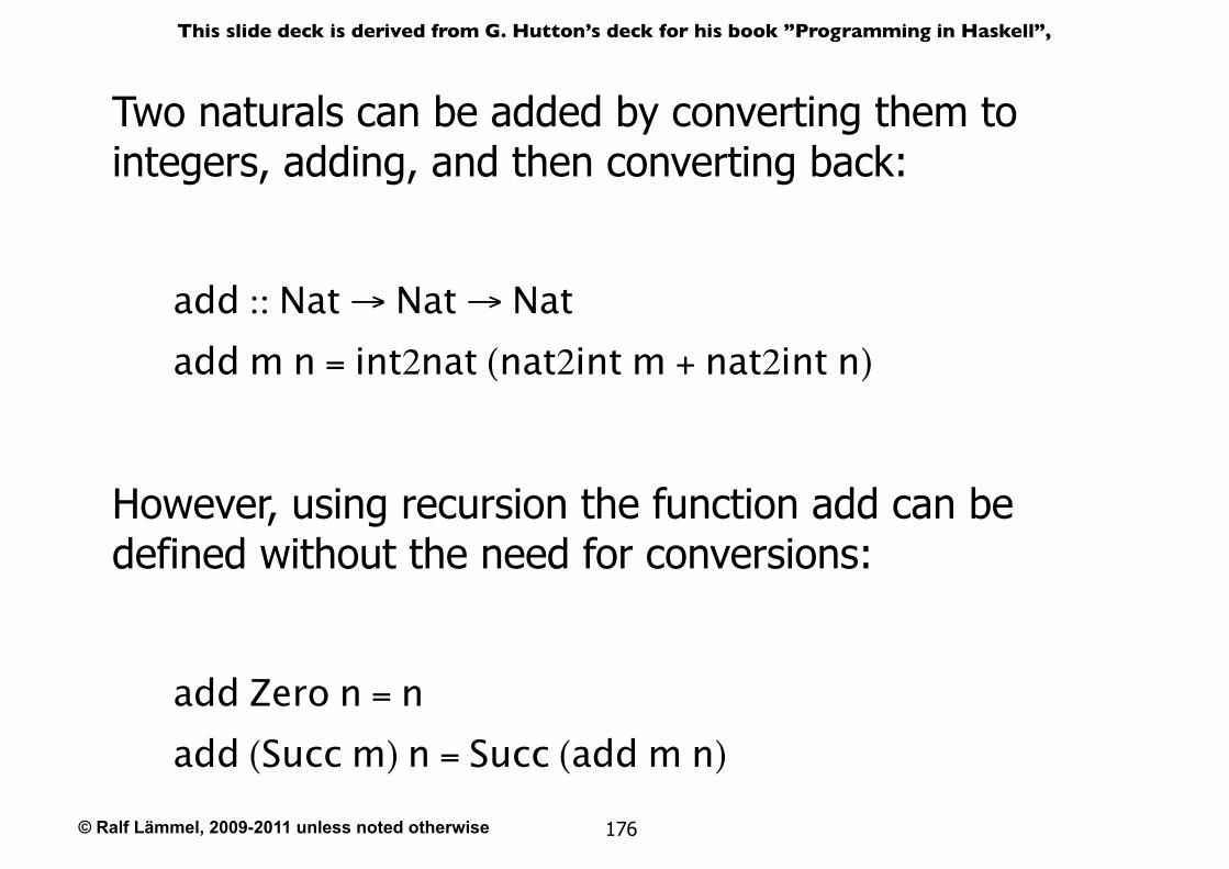
Two naturals can be added by converting them to integers, adding, and then converting back:
However, using recursion the function add can be defined without the need for conversions:
add :: Nat → Nat → Natadd m n = int2nat (nat2int m + nat2int n)
add Zero n = nadd (Succ m) n = Succ (add m n)
© Ralf Lämmel, 2009-2011 unless noted otherwise
This slide deck is derived from G. Hutton’s deck for his book ”Programming in Haskell”,
177
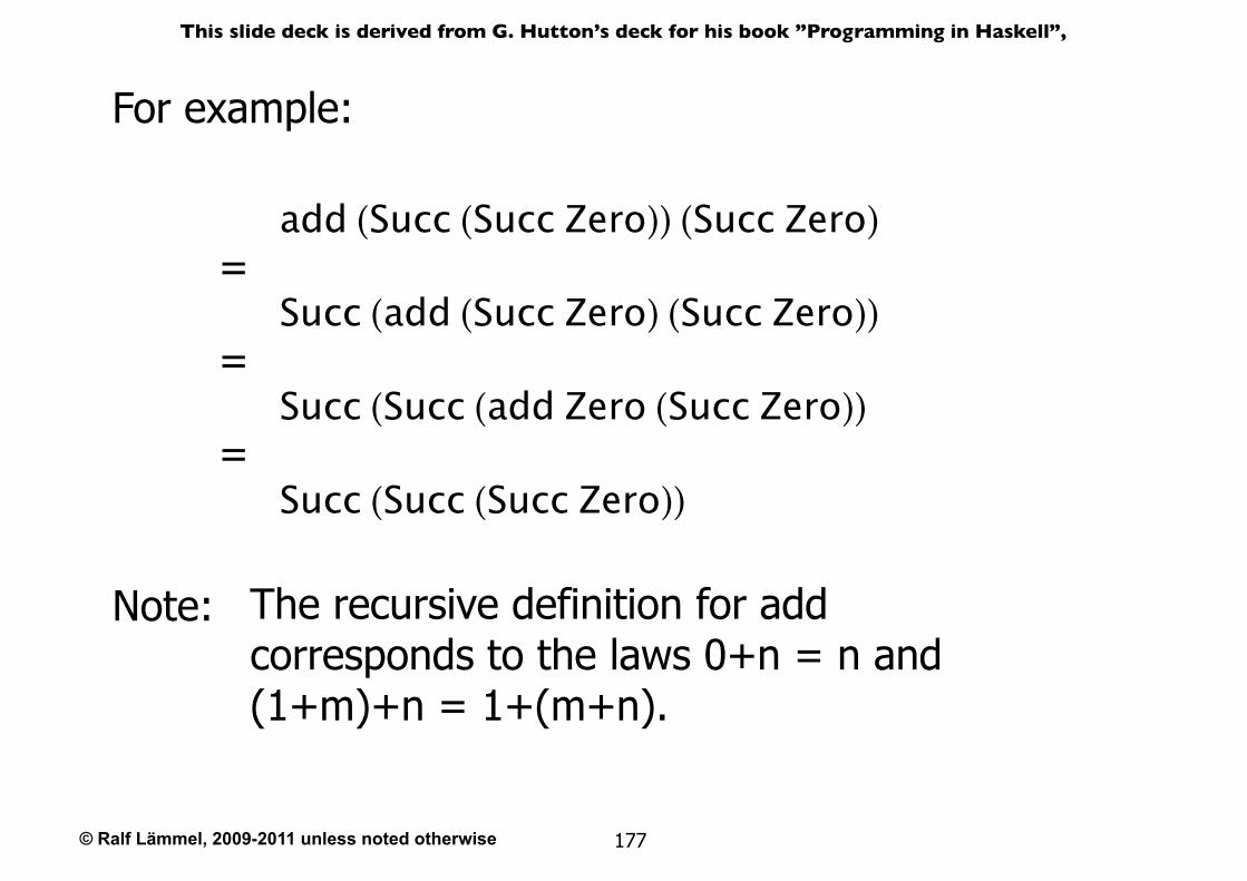
For example:
add (Succ (Succ Zero)) (Succ Zero)
Succ (add (Succ Zero) (Succ Zero))=
Succ (Succ (add Zero (Succ Zero))=
Succ (Succ (Succ Zero))=
Note: The recursive definition for add corresponds to the laws 0+n = n and (1+m)+n = 1+(m+n).
© Ralf Lämmel, 2009-2011 unless noted otherwise
This slide deck is derived from G. Hutton’s deck for his book ”Programming in Haskell”,
178
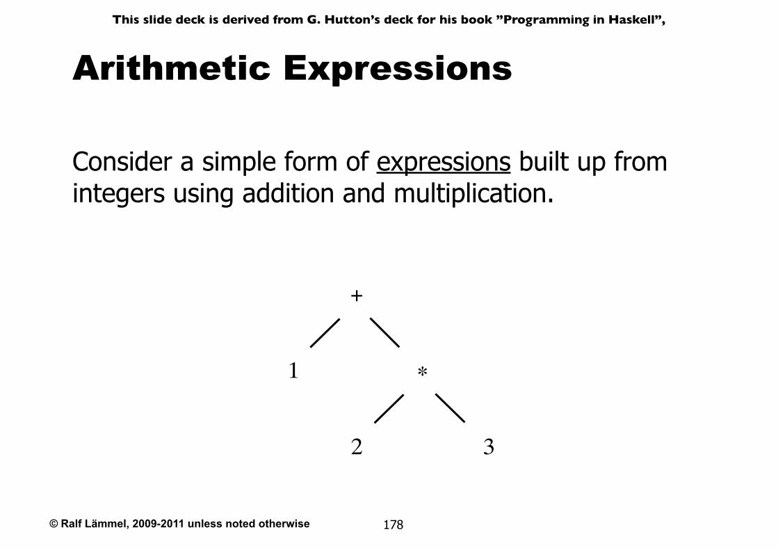
Arithmetic Expressions
Consider a simple form of expressions built up from integers using addition and multiplication.
1
+
∗
32
© Ralf Lämmel, 2009-2011 unless noted otherwise
This slide deck is derived from G. Hutton’s deck for his book ”Programming in Haskell”,
179
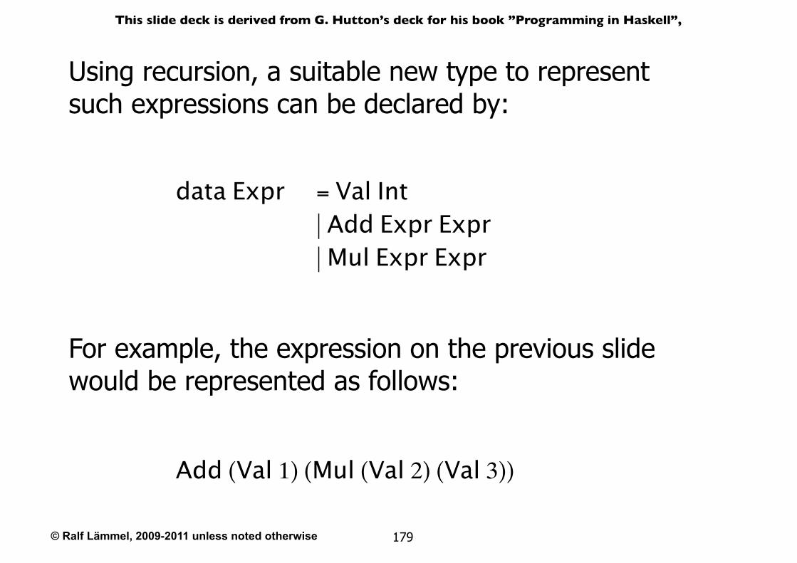
Using recursion, a suitable new type to represent such expressions can be declared by:
For example, the expression on the previous slide would be represented as follows:
data Expr = Val Int | Add Expr Expr | Mul Expr Expr
Add (Val 1) (Mul (Val 2) (Val 3))
© Ralf Lämmel, 2009-2011 unless noted otherwise
This slide deck is derived from G. Hutton’s deck for his book ”Programming in Haskell”,
180
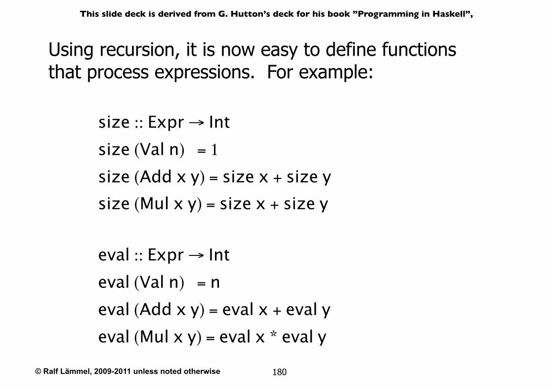
Using recursion, it is now easy to define functions that process expressions. For example:
size :: Expr → Intsize (Val n) = 1
size (Add x y) = size x + size ysize (Mul x y) = size x + size y
eval :: Expr → Inteval (Val n) = neval (Add x y) = eval x + eval yeval (Mul x y) = eval x * eval y
© Ralf Lämmel, 2009-2011 unless noted otherwise
This slide deck is derived from G. Hutton’s deck for his book ”Programming in Haskell”,
181
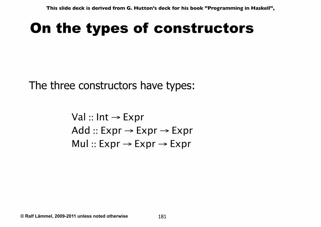
The three constructors have types:
Val :: Int → ExprAdd :: Expr → Expr → ExprMul :: Expr → Expr → Expr
On the types of constructors
© Ralf Lämmel, 2009-2011 unless noted otherwise
This slide deck is derived from G. Hutton’s deck for his book ”Programming in Haskell”,
182
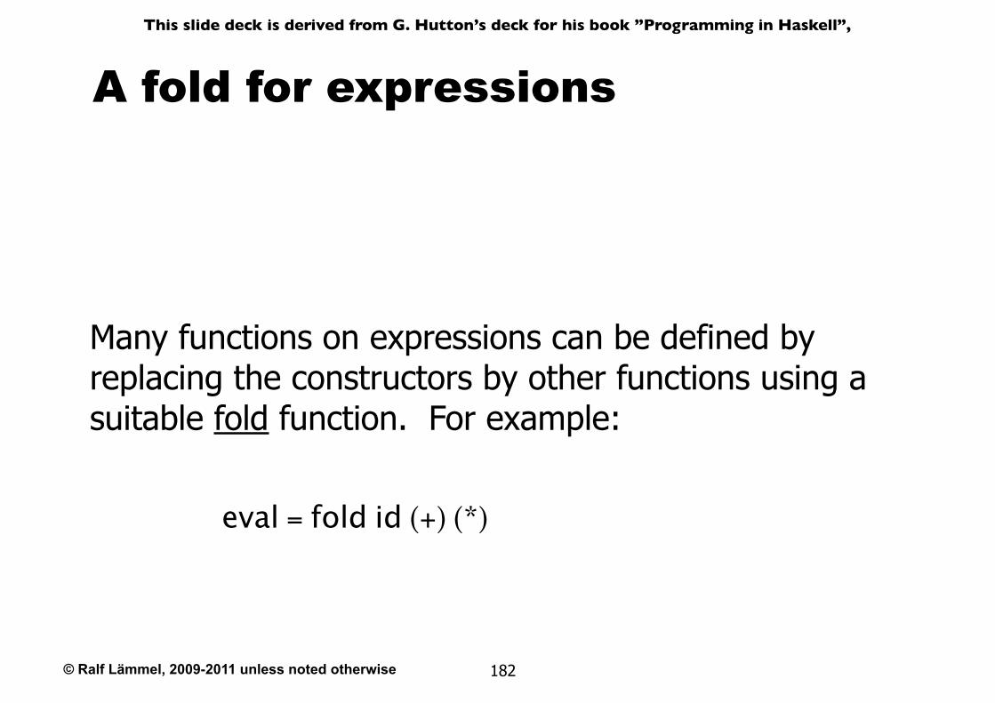
Many functions on expressions can be defined by replacing the constructors by other functions using a suitable fold function. For example:
eval = fold id (+) (*)
A fold for expressions
© Ralf Lämmel, 2009-2011 unless noted otherwise
This slide deck is derived from G. Hutton’s deck for his book ”Programming in Haskell”,
183
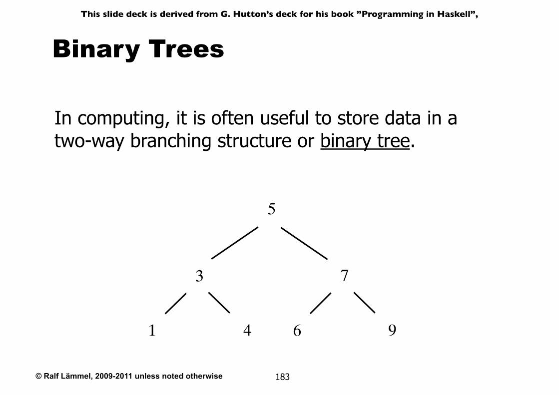
Binary Trees
In computing, it is often useful to store data in a two-way branching structure or binary tree.
5
7
96
3
41
© Ralf Lämmel, 2009-2011 unless noted otherwise
This slide deck is derived from G. Hutton’s deck for his book ”Programming in Haskell”,
184
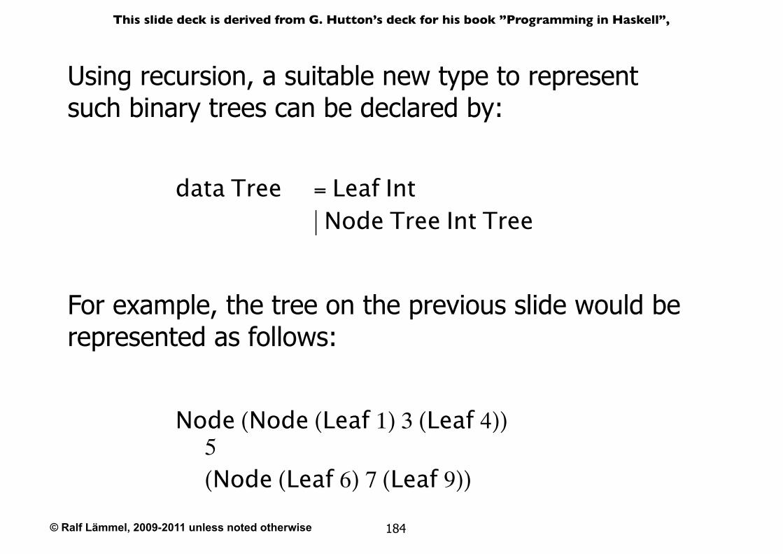
Using recursion, a suitable new type to represent such binary trees can be declared by:
For example, the tree on the previous slide would be represented as follows:
data Tree = Leaf Int | Node Tree Int Tree
Node (Node (Leaf 1) 3 (Leaf 4)) 5 (Node (Leaf 6) 7 (Leaf 9))
© Ralf Lämmel, 2009-2011 unless noted otherwise
This slide deck is derived from G. Hutton’s deck for his book ”Programming in Haskell”,
185
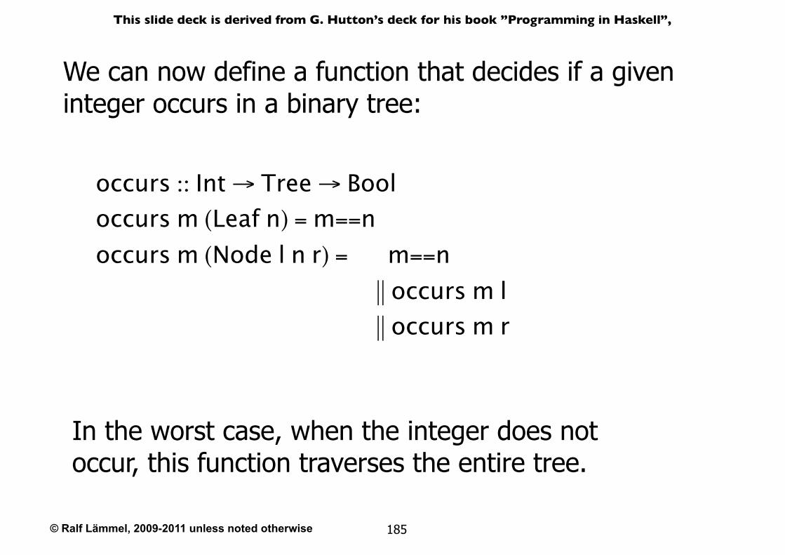
We can now define a function that decides if a given integer occurs in a binary tree:
occurs :: Int → Tree → Booloccurs m (Leaf n) = m==noccurs m (Node l n r) = m==n || occurs m l || occurs m r
In the worst case, when the integer does not occur, this function traverses the entire tree.
© Ralf Lämmel, 2009-2011 unless noted otherwise
This slide deck is derived from G. Hutton’s deck for his book ”Programming in Haskell”,
186
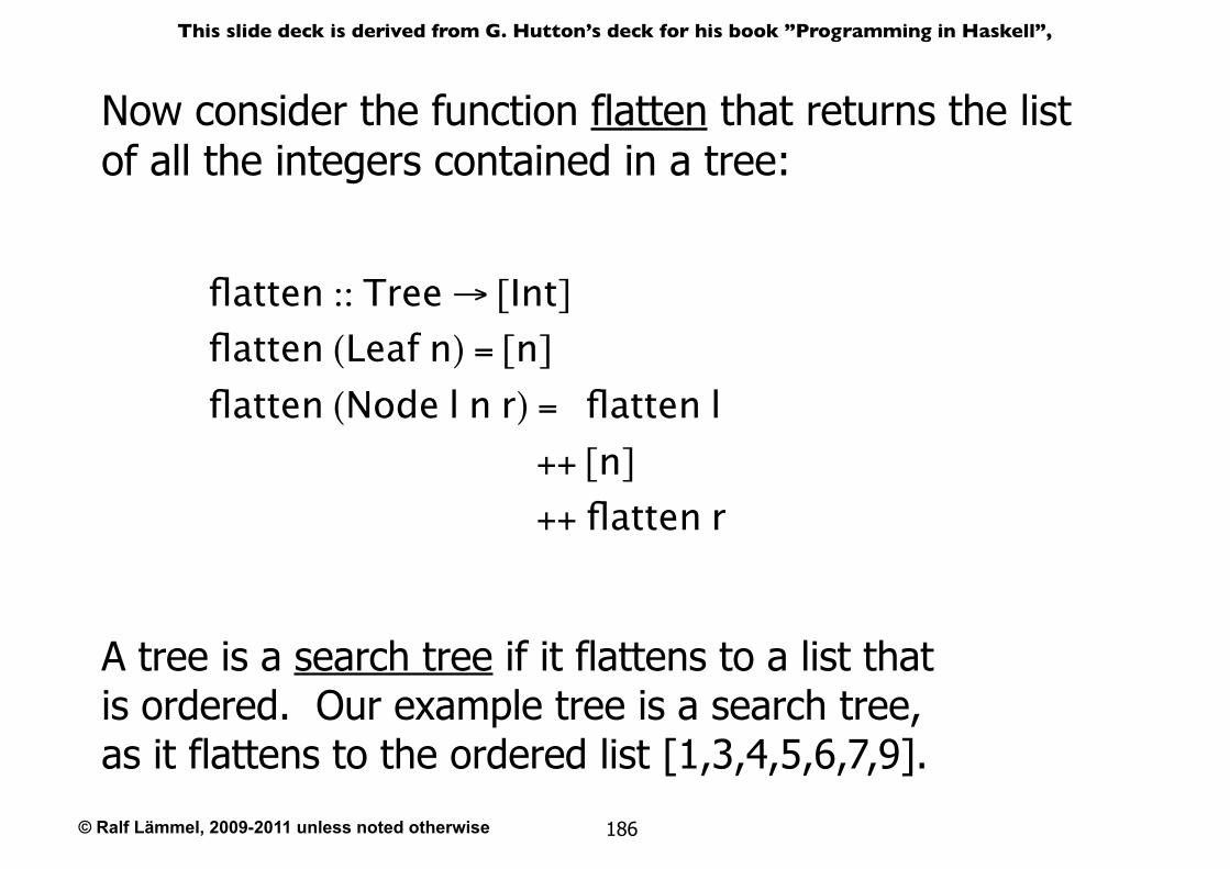
Now consider the function flatten that returns the list of all the integers contained in a tree:
flatten :: Tree → [Int]flatten (Leaf n) = [n]
flatten (Node l n r) = flatten l ++ [n]
++ flatten r
A tree is a search tree if it flattens to a list that is ordered. Our example tree is a search tree, as it flattens to the ordered list [1,3,4,5,6,7,9].
© Ralf Lämmel, 2009-2011 unless noted otherwise
This slide deck is derived from G. Hutton’s deck for his book ”Programming in Haskell”,
187
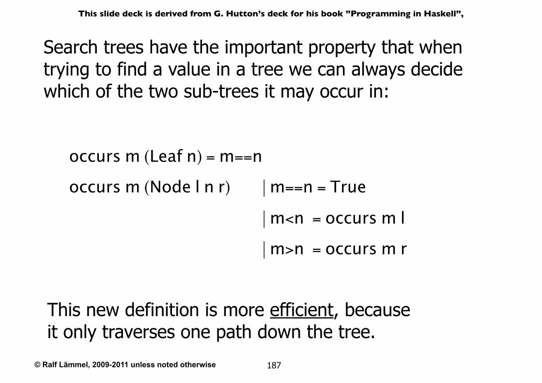
Search trees have the important property that when trying to find a value in a tree we can always decide which of the two sub-trees it may occur in:
This new definition is more efficient, because it only traverses one path down the tree.
occurs m (Leaf n) = m==n
occurs m (Node l n r) | m==n = True
| m<n = occurs m l
| m>n = occurs m r
© Ralf Lämmel, 2009-2011 unless noted otherwise
This slide deck is derived from G. Hutton’s deck for his book ”Programming in Haskell”,
188
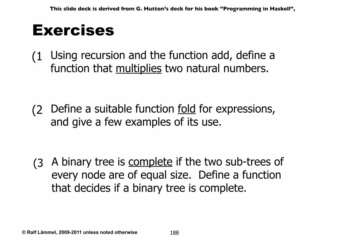
Exercises(1 Using recursion and the function add, define a
function that multiplies two natural numbers.
(2 Define a suitable function fold for expressions, and give a few examples of its use.
(3 A binary tree is complete if the two sub-trees of every node are of equal size. Define a function that decides if a binary tree is complete.
© Ralf Lämmel, 2009-2011 unless noted otherwise
This slide deck is derived from G. Hutton’s deck for his book ”Programming in Haskell”,
189
Functional Parsers
© Ralf Lämmel, 2009-2011 unless noted otherwise
This slide deck is derived from G. Hutton’s deck for his book ”Programming in Haskell”,
190
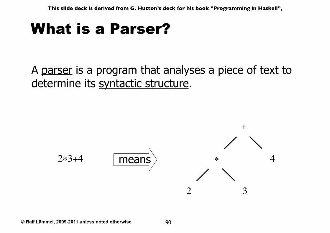
What is a Parser?
A parser is a program that analyses a piece of text to determine its syntactic structure.
2∗3+4 means 4
+
2
∗
32
© Ralf Lämmel, 2009-2011 unless noted otherwise
This slide deck is derived from G. Hutton’s deck for his book ”Programming in Haskell”,
191
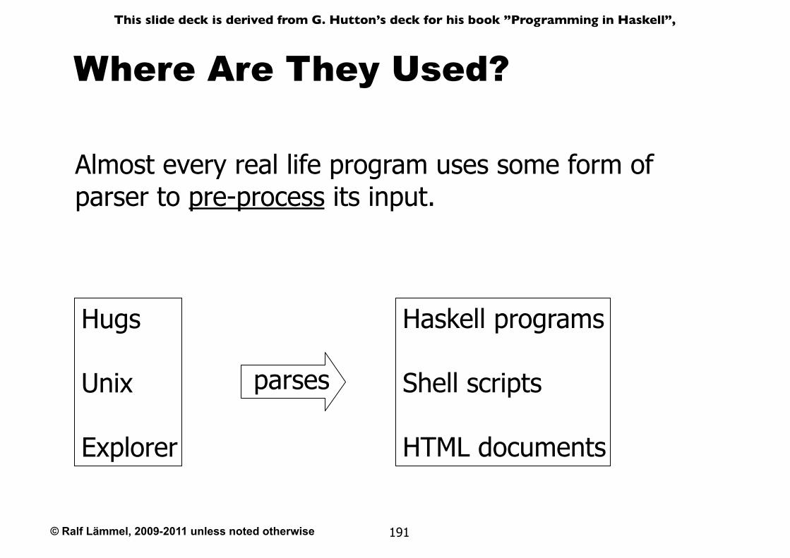
Where Are They Used?
Almost every real life program uses some form of parser to pre-process its input.
Haskell programs
Shell scripts
HTML documents
Hugs
Unix
Explorer
parses
© Ralf Lämmel, 2009-2011 unless noted otherwise
This slide deck is derived from G. Hutton’s deck for his book ”Programming in Haskell”,
192
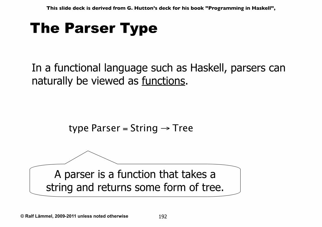
The Parser Type
In a functional language such as Haskell, parsers can naturally be viewed as functions.
type Parser = String → Tree
A parser is a function that takes a string and returns some form of tree.
© Ralf Lämmel, 2009-2011 unless noted otherwise
This slide deck is derived from G. Hutton’s deck for his book ”Programming in Haskell”,
193
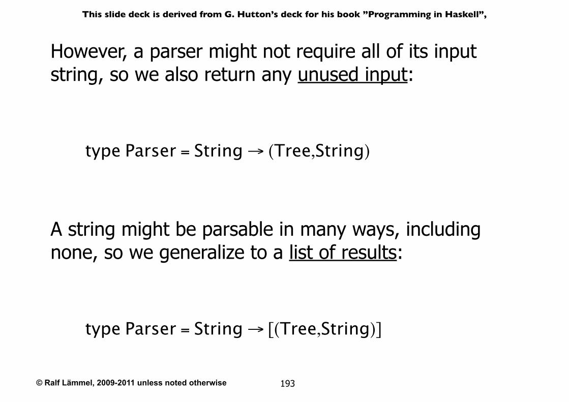
However, a parser might not require all of its input string, so we also return any unused input:
type Parser = String → (Tree,String)
A string might be parsable in many ways, including none, so we generalize to a list of results:
type Parser = String → [(Tree,String)]
© Ralf Lämmel, 2009-2011 unless noted otherwise
This slide deck is derived from G. Hutton’s deck for his book ”Programming in Haskell”,
194
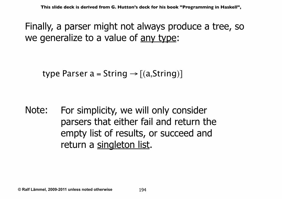
Finally, a parser might not always produce a tree, so we generalize to a value of any type:
type Parser a = String → [(a,String)]
Note: For simplicity, we will only consider parsers that either fail and return the empty list of results, or succeed and return a singleton list.
© Ralf Lämmel, 2009-2011 unless noted otherwise
This slide deck is derived from G. Hutton’s deck for his book ”Programming in Haskell”,
195
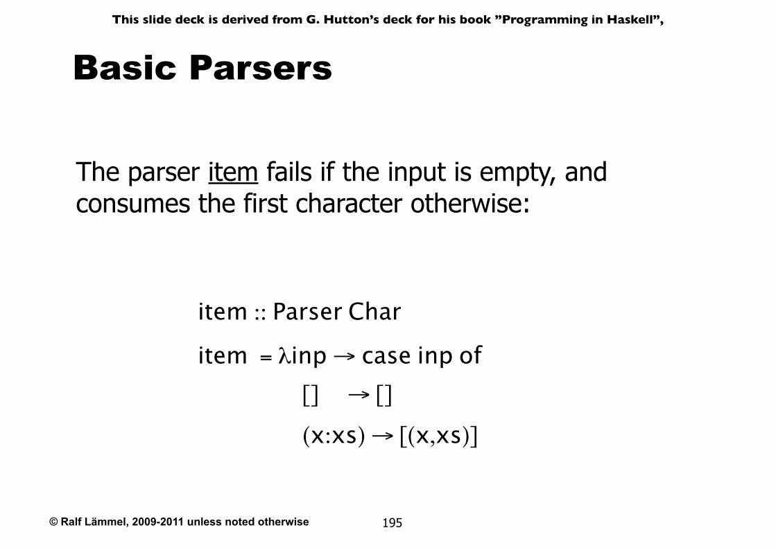
Basic Parsers
The parser item fails if the input is empty, and consumes the first character otherwise:
item :: Parser Char
item = λinp → case inp of [] → []
(x:xs) → [(x,xs)]
© Ralf Lämmel, 2009-2011 unless noted otherwise
This slide deck is derived from G. Hutton’s deck for his book ”Programming in Haskell”,
196
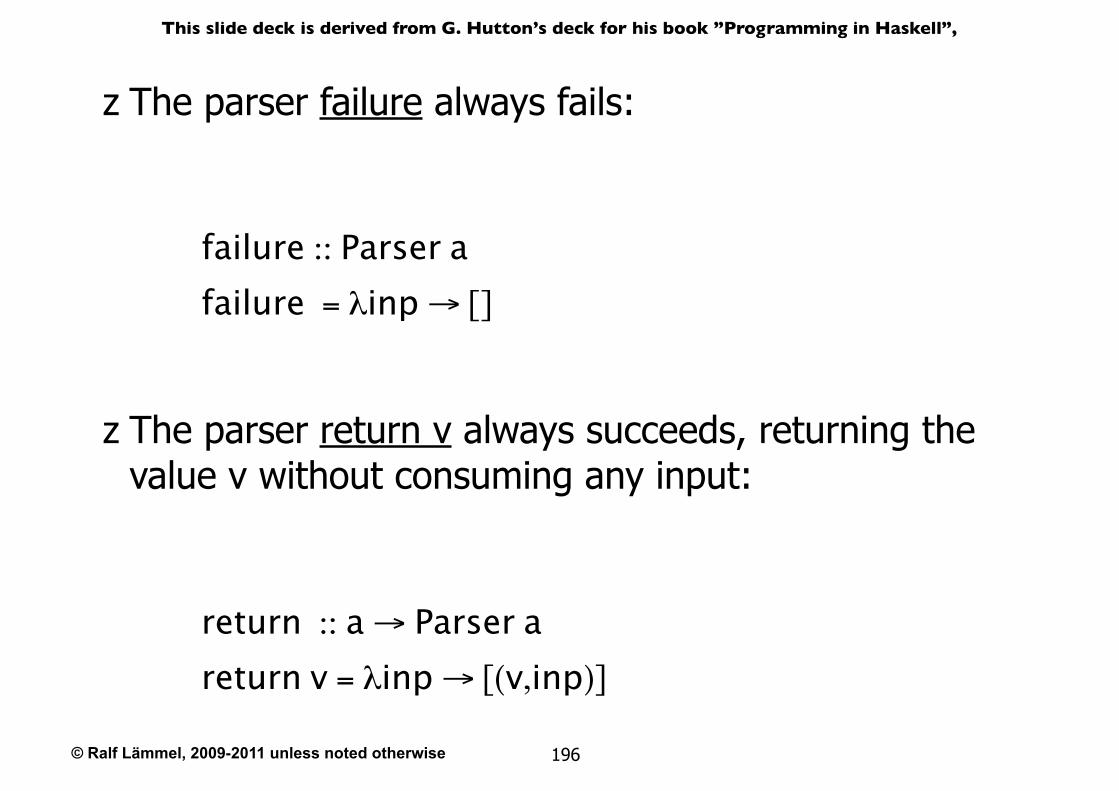
z The parser failure always fails:
failure :: Parser afailure = λinp → []
z The parser return v always succeeds, returning the value v without consuming any input:
return :: a → Parser areturn v = λinp → [(v,inp)]
© Ralf Lämmel, 2009-2011 unless noted otherwise
This slide deck is derived from G. Hutton’s deck for his book ”Programming in Haskell”,
197
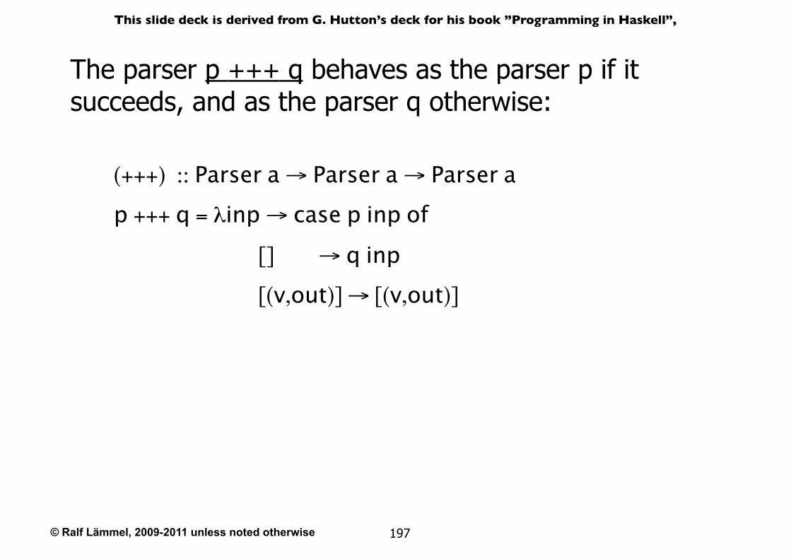
The parser p +++ q behaves as the parser p if it succeeds, and as the parser q otherwise:
(+++) :: Parser a → Parser a → Parser ap +++ q = λinp → case p inp of
[] → q inp [(v,out)] → [(v,out)]
© Ralf Lämmel, 2009-2011 unless noted otherwise
This slide deck is derived from G. Hutton’s deck for his book ”Programming in Haskell”,
198
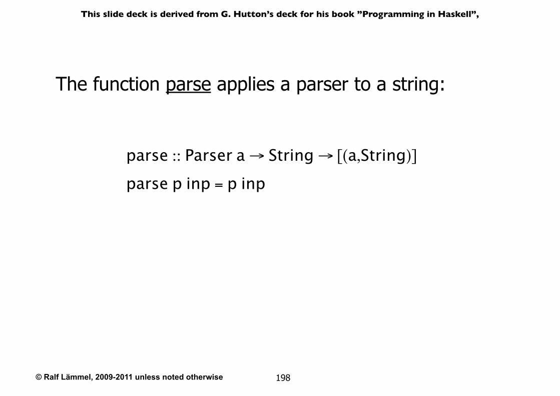
The function parse applies a parser to a string:
parse :: Parser a → String → [(a,String)]
parse p inp = p inp
© Ralf Lämmel, 2009-2011 unless noted otherwise
This slide deck is derived from G. Hutton’s deck for his book ”Programming in Haskell”,
199
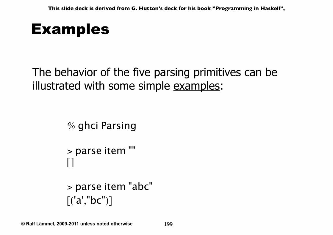
Examples
% ghci Parsing
> parse item ""[]
> parse item "abc"[('a',"bc")]
The behavior of the five parsing primitives can be illustrated with some simple examples:
© Ralf Lämmel, 2009-2011 unless noted otherwise
This slide deck is derived from G. Hutton’s deck for his book ”Programming in Haskell”,
200
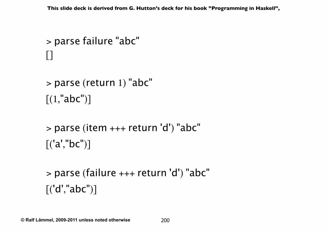
> parse failure "abc"[]
> parse (return 1) "abc"[(1,"abc")]
> parse (item +++ return 'd') "abc"[('a',"bc")]
> parse (failure +++ return 'd') "abc"[('d',"abc")]
© Ralf Lämmel, 2009-2011 unless noted otherwise
This slide deck is derived from G. Hutton’s deck for his book ”Programming in Haskell”,
201
Note:
๏The library file Parsing is available on the web from the Programming in Haskell home page.
๏For technical reasons, the first failure example actually gives an error concerning types, but this does not occur in non-trivial examples.
๏The Parser type is a monad, a mathematical structure that has proved useful for modeling many different kinds of computations.
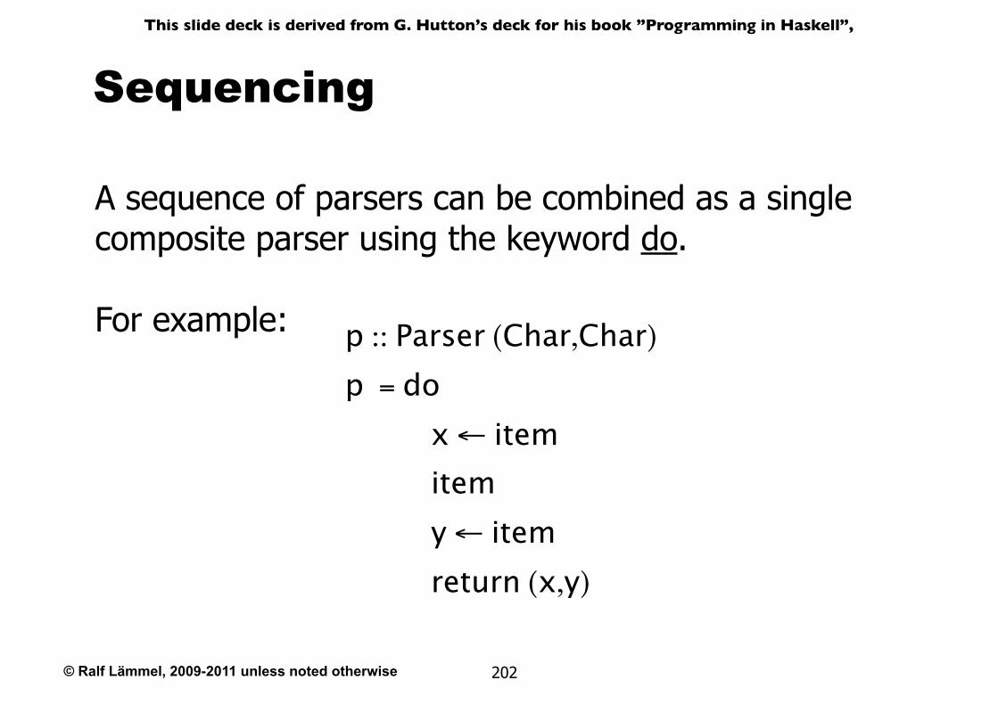
© Ralf Lämmel, 2009-2011 unless noted otherwise
This slide deck is derived from G. Hutton’s deck for his book ”Programming in Haskell”,
202
A sequence of parsers can be combined as a single composite parser using the keyword do.
For example:
Sequencing
p :: Parser (Char,Char)p = do
x ← item item y ← item return (x,y)
© Ralf Lämmel, 2009-2011 unless noted otherwise
This slide deck is derived from G. Hutton’s deck for his book ”Programming in Haskell”,
203
Note:
๏Each parser must begin in precisely the same column. That is, the layout rule applies.
๏The values returned by intermediate parsers are discarded by default, but if required can be named using the ← operator.
๏The value returned by the last parser is the value returned by the sequence as a whole.
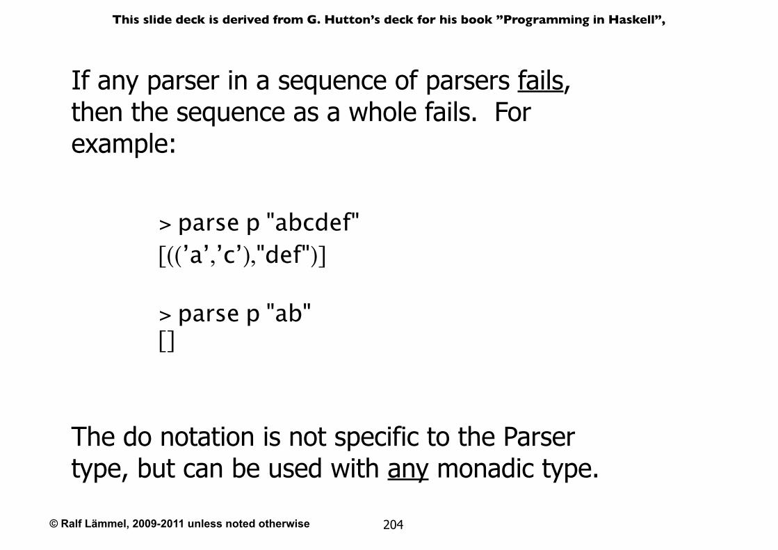
© Ralf Lämmel, 2009-2011 unless noted otherwise
This slide deck is derived from G. Hutton’s deck for his book ”Programming in Haskell”,
204
If any parser in a sequence of parsers fails, then the sequence as a whole fails. For example:
> parse p "abcdef"[((’a’,’c’),"def")]
> parse p "ab"[]
The do notation is not specific to the Parser type, but can be used with any monadic type.
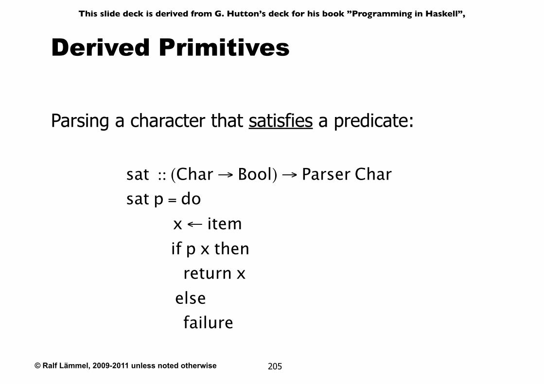
© Ralf Lämmel, 2009-2011 unless noted otherwise
This slide deck is derived from G. Hutton’s deck for his book ”Programming in Haskell”,
205
Derived Primitives
sat :: (Char → Bool) → Parser Charsat p = do
x ← item if p x then return x else failure
Parsing a character that satisfies a predicate:
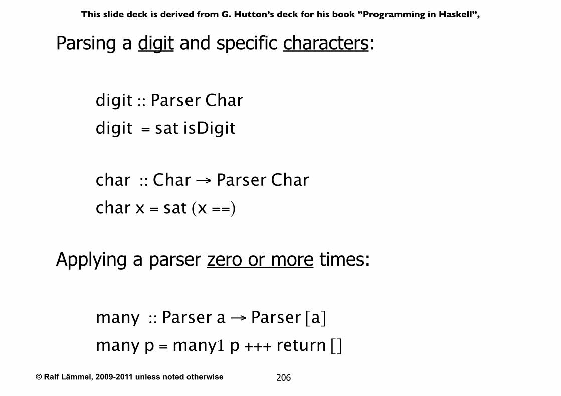
© Ralf Lämmel, 2009-2011 unless noted otherwise
This slide deck is derived from G. Hutton’s deck for his book ”Programming in Haskell”,
206
digit :: Parser Chardigit = sat isDigit
char :: Char → Parser Charchar x = sat (x ==)
Parsing a digit and specific characters:
Applying a parser zero or more times:
many :: Parser a → Parser [a]
many p = many1 p +++ return []
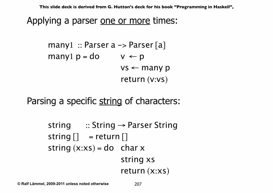
© Ralf Lämmel, 2009-2011 unless noted otherwise
This slide deck is derived from G. Hutton’s deck for his book ”Programming in Haskell”,
207
many1 :: Parser a -> Parser [a]many1 p = do v ← p vs ← many p return (v:vs)
Applying a parser one or more times:
Parsing a specific string of characters:
string :: String → Parser Stringstring [] = return []string (x:xs) = do char x string xs return (x:xs)
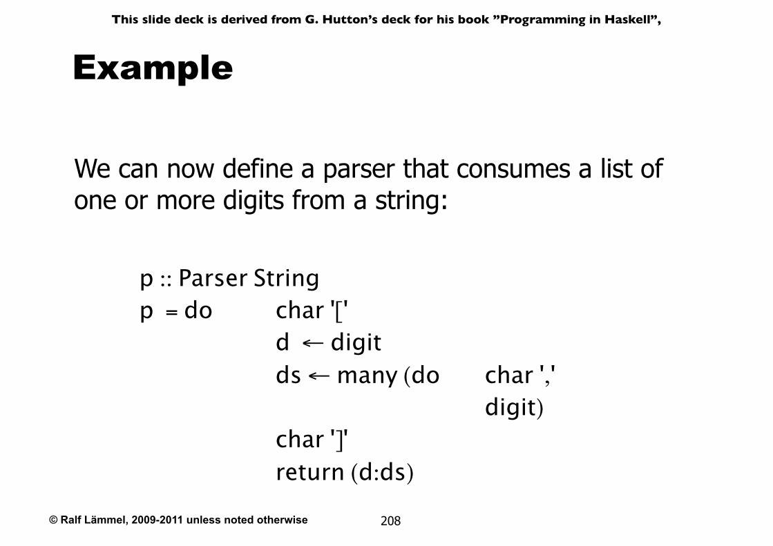
© Ralf Lämmel, 2009-2011 unless noted otherwise
This slide deck is derived from G. Hutton’s deck for his book ”Programming in Haskell”,
208
Example
We can now define a parser that consumes a list of one or more digits from a string:
p :: Parser Stringp = do char '[' d ← digit ds ← many (do char ',' digit) char ']' return (d:ds)
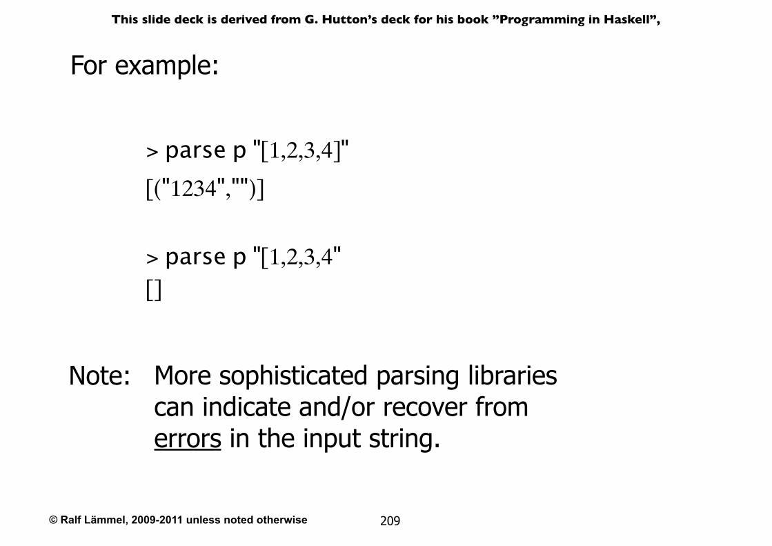
© Ralf Lämmel, 2009-2011 unless noted otherwise
This slide deck is derived from G. Hutton’s deck for his book ”Programming in Haskell”,
209
For example:
> parse p "[1,2,3,4]"[("1234","")]
> parse p "[1,2,3,4"[]
Note: More sophisticated parsing libraries can indicate and/or recover from errors in the input string.
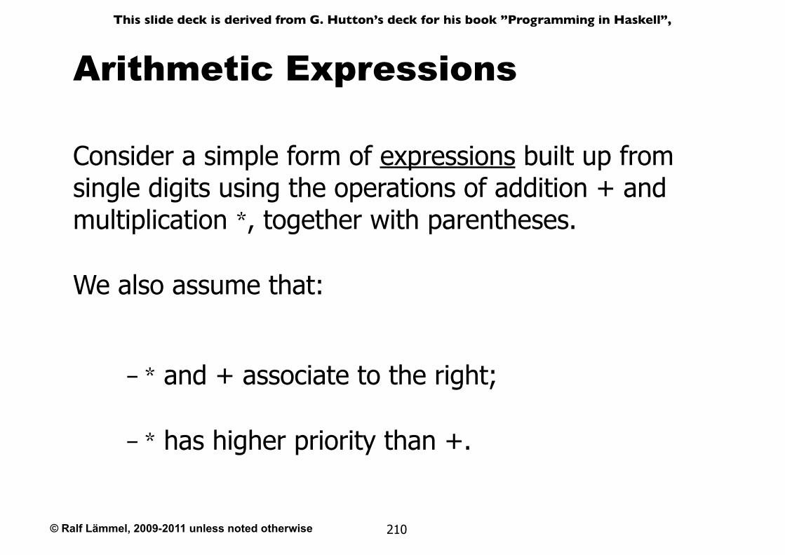
© Ralf Lämmel, 2009-2011 unless noted otherwise
This slide deck is derived from G. Hutton’s deck for his book ”Programming in Haskell”,
210
Arithmetic Expressions
Consider a simple form of expressions built up from single digits using the operations of addition + and multiplication *, together with parentheses.
We also assume that:
- * and + associate to the right;
- * has higher priority than +.
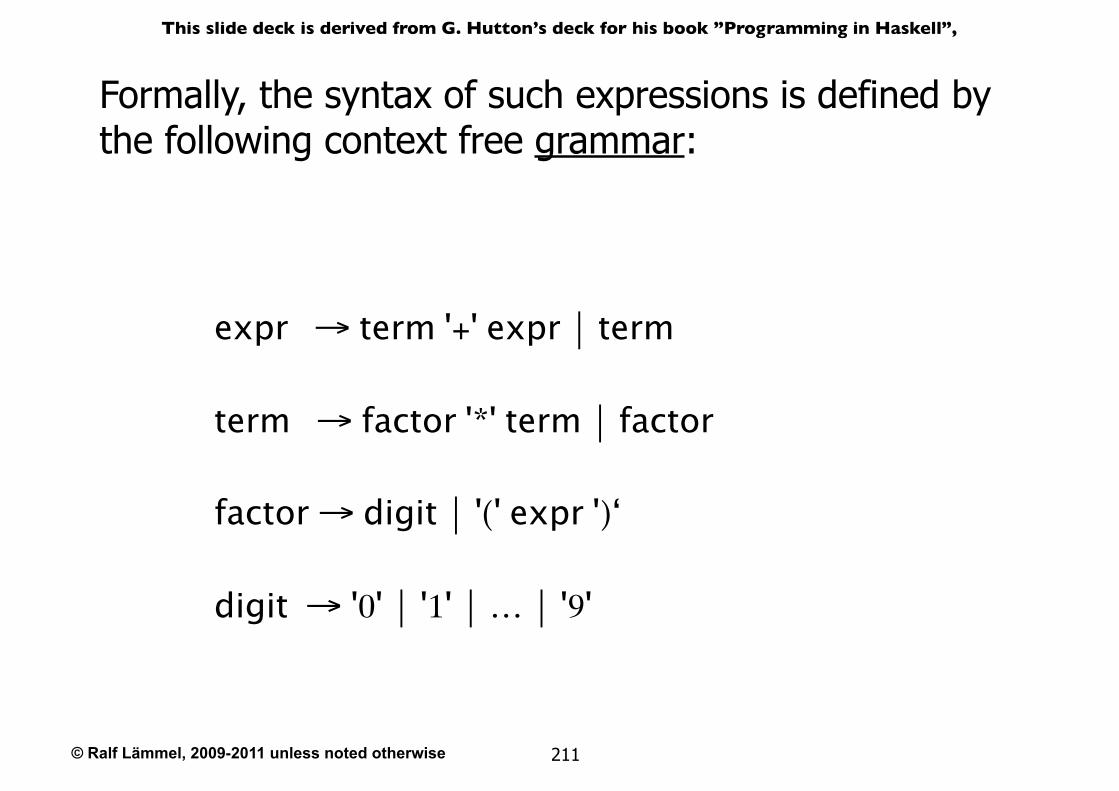
© Ralf Lämmel, 2009-2011 unless noted otherwise
This slide deck is derived from G. Hutton’s deck for his book ”Programming in Haskell”,
211
Formally, the syntax of such expressions is defined by the following context free grammar:
expr → term '+' expr ⏐ term
term → factor '*' term ⏐ factor
factor → digit ⏐ '(' expr ')‘
digit → '0' ⏐ '1' ⏐ … ⏐ '9'
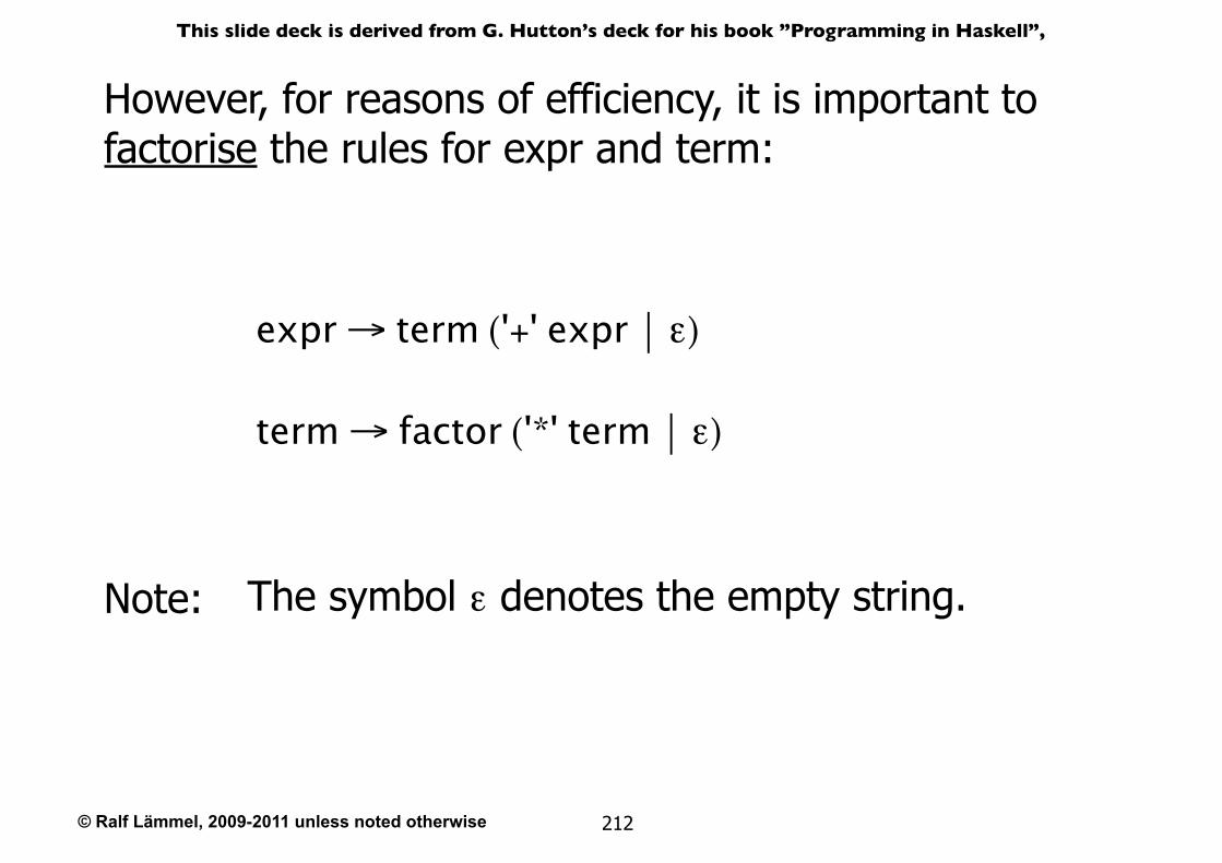
© Ralf Lämmel, 2009-2011 unless noted otherwise
This slide deck is derived from G. Hutton’s deck for his book ”Programming in Haskell”,
212
However, for reasons of efficiency, it is important to factorise the rules for expr and term:
expr → term ('+' expr ⏐ ε)
term → factor ('*' term ⏐ ε)
Note: The symbol ε denotes the empty string.
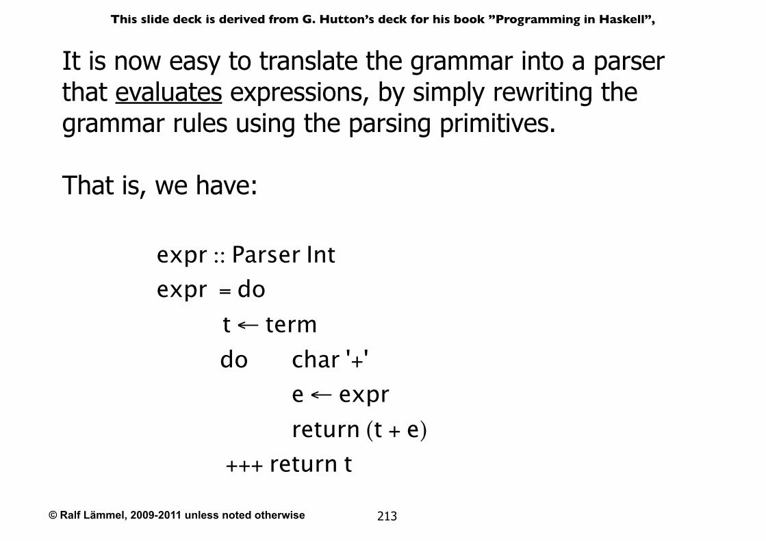
© Ralf Lämmel, 2009-2011 unless noted otherwise
This slide deck is derived from G. Hutton’s deck for his book ”Programming in Haskell”,
213
It is now easy to translate the grammar into a parser that evaluates expressions, by simply rewriting the grammar rules using the parsing primitives.
That is, we have:
expr :: Parser Intexpr = do
t ← term do char '+' e ← expr return (t + e)
+++ return t
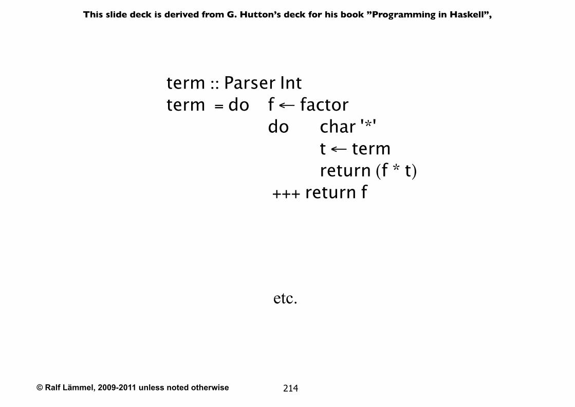
© Ralf Lämmel, 2009-2011 unless noted otherwise
This slide deck is derived from G. Hutton’s deck for his book ”Programming in Haskell”,
214
term :: Parser Intterm = do f ← factor do char '*' t ← term return (f * t) +++ return f
etc.
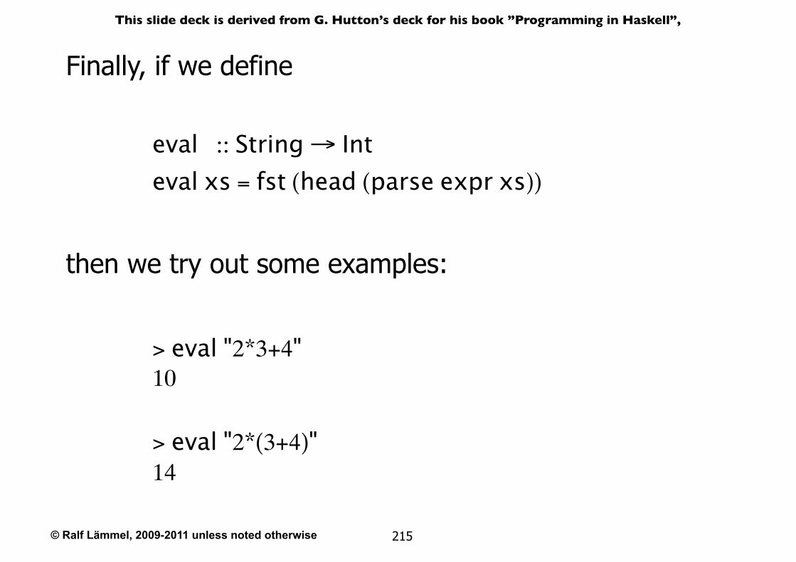
© Ralf Lämmel, 2009-2011 unless noted otherwise
This slide deck is derived from G. Hutton’s deck for his book ”Programming in Haskell”,
215
Finally, if we define
eval :: String → Inteval xs = fst (head (parse expr xs))
then we try out some examples:
> eval "2*3+4"10
> eval "2*(3+4)"14
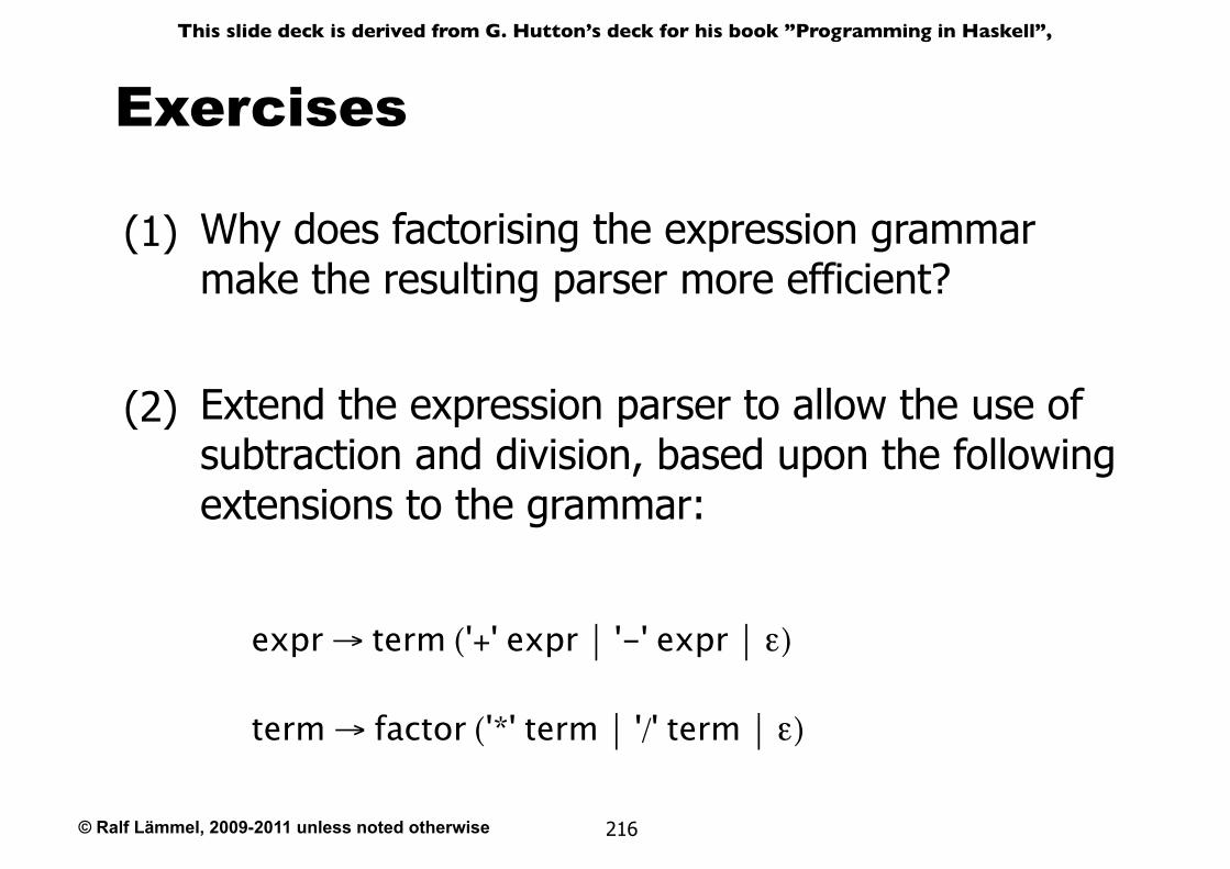
© Ralf Lämmel, 2009-2011 unless noted otherwise
This slide deck is derived from G. Hutton’s deck for his book ”Programming in Haskell”,
216
Exercises
(2) Extend the expression parser to allow the use of subtraction and division, based upon the following extensions to the grammar:
expr → term ('+' expr ⏐ '-' expr ⏐ ε)
term → factor ('*' term ⏐ '/' term ⏐ ε)
(1) Why does factorising the expression grammar make the resulting parser more efficient?
© Ralf Lämmel, 2009-2011 unless noted otherwise
This slide deck is derived from G. Hutton’s deck for his book ”Programming in Haskell”,
217
Interactive Programs

© Ralf Lämmel, 2009-2011 unless noted otherwise
This slide deck is derived from G. Hutton’s deck for his book ”Programming in Haskell”,
218
Introduction
To date, we have seen how Haskell can be used to write batch programs that take all their inputs at the start and give all their outputs at the end.
batchprogram
inputs outputs
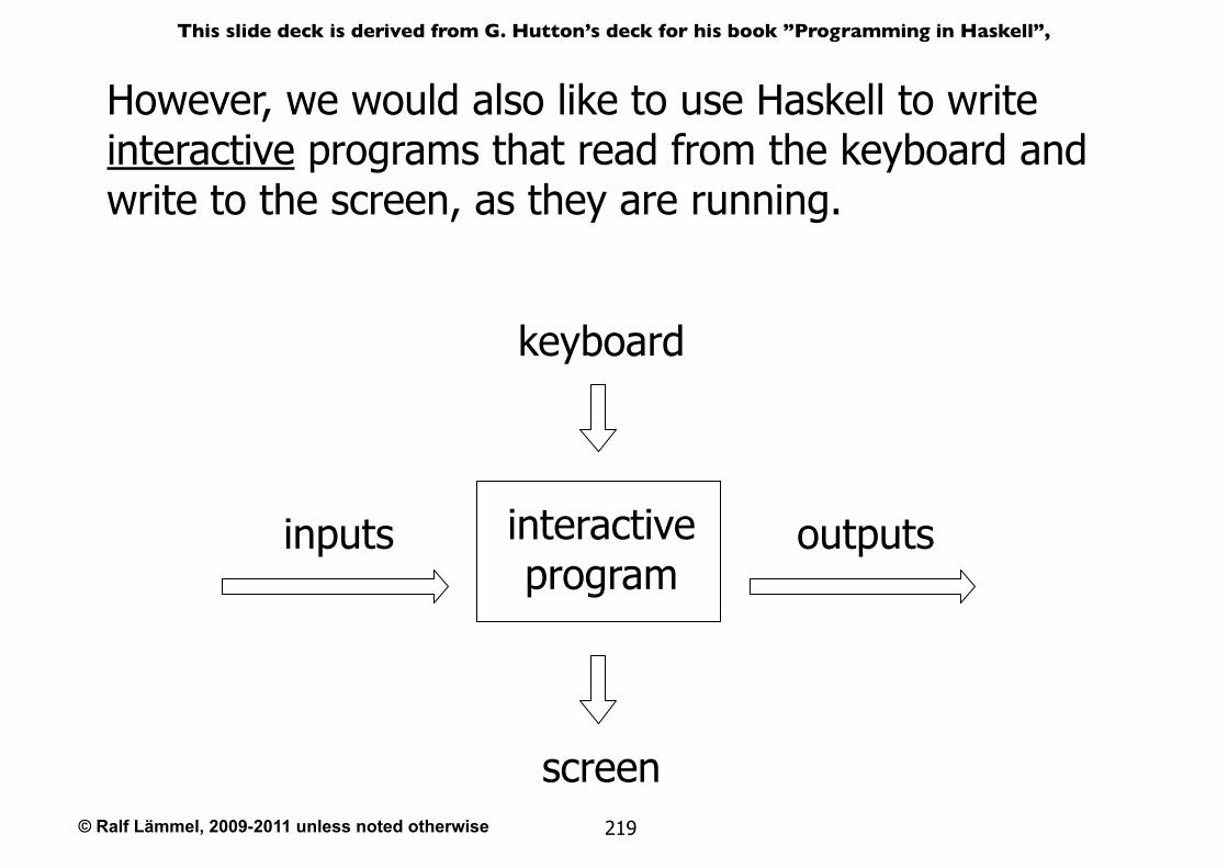
© Ralf Lämmel, 2009-2011 unless noted otherwise
This slide deck is derived from G. Hutton’s deck for his book ”Programming in Haskell”,
219
However, we would also like to use Haskell to write interactive programs that read from the keyboard and write to the screen, as they are running.
interactiveprogram
inputs outputs
keyboard
screen
© Ralf Lämmel, 2009-2011 unless noted otherwise
This slide deck is derived from G. Hutton’s deck for his book ”Programming in Haskell”,
220
The Problem
Haskell programs are pure mathematical functions:
However, reading from the keyboard and writing to the screen are side effects:
Haskell programs have no side effects.
Interactive programs have side effects.
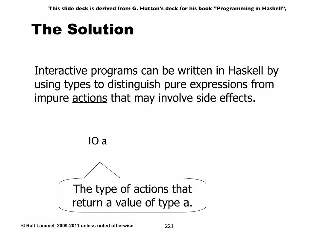
© Ralf Lämmel, 2009-2011 unless noted otherwise
This slide deck is derived from G. Hutton’s deck for his book ”Programming in Haskell”,
221
The Solution
Interactive programs can be written in Haskell by using types to distinguish pure expressions from impure actions that may involve side effects.
IO a
The type of actions that return a value of type a.
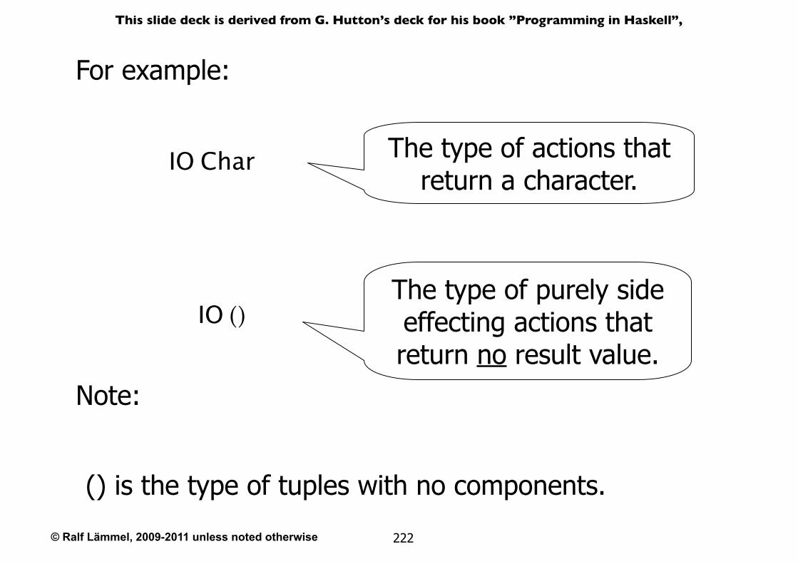
© Ralf Lämmel, 2009-2011 unless noted otherwise
This slide deck is derived from G. Hutton’s deck for his book ”Programming in Haskell”,
222
For example:
IO Char
IO ()
The type of actions that return a character.
The type of purely side effecting actions that return no result value.
() is the type of tuples with no components.
Note:
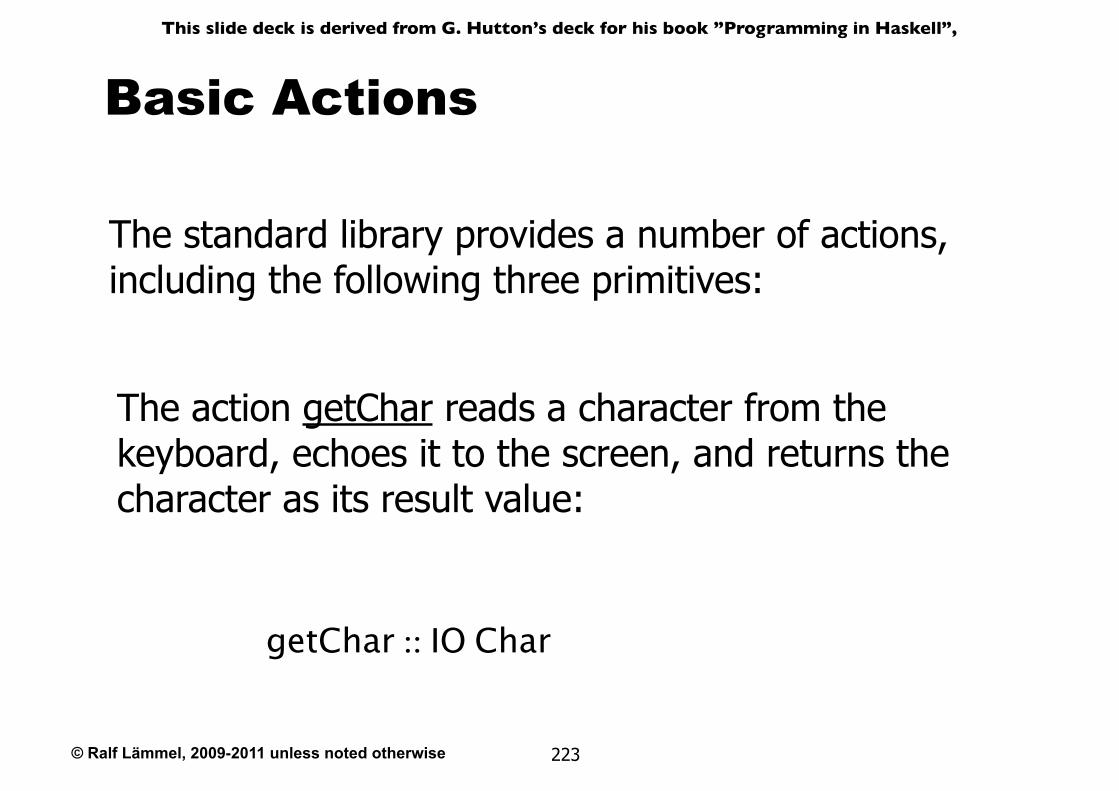
© Ralf Lämmel, 2009-2011 unless noted otherwise
This slide deck is derived from G. Hutton’s deck for his book ”Programming in Haskell”,
223
Basic Actions
The standard library provides a number of actions, including the following three primitives:
getChar :: IO Char
The action getChar reads a character from the keyboard, echoes it to the screen, and returns the character as its result value:
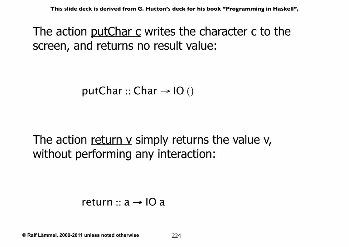
© Ralf Lämmel, 2009-2011 unless noted otherwise
This slide deck is derived from G. Hutton’s deck for his book ”Programming in Haskell”,
224
The action putChar c writes the character c to the screen, and returns no result value:
putChar :: Char → IO ()
The action return v simply returns the value v, without performing any interaction:
return :: a → IO a
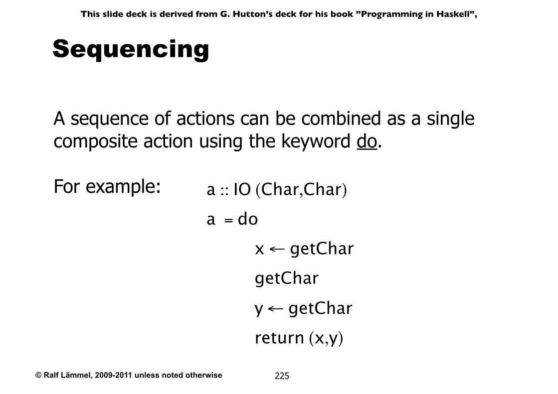
© Ralf Lämmel, 2009-2011 unless noted otherwise
This slide deck is derived from G. Hutton’s deck for his book ”Programming in Haskell”,
225
A sequence of actions can be combined as a single composite action using the keyword do.
For example:
Sequencing
a :: IO (Char,Char)a = do
x ← getChar getChar y ← getChar return (x,y)
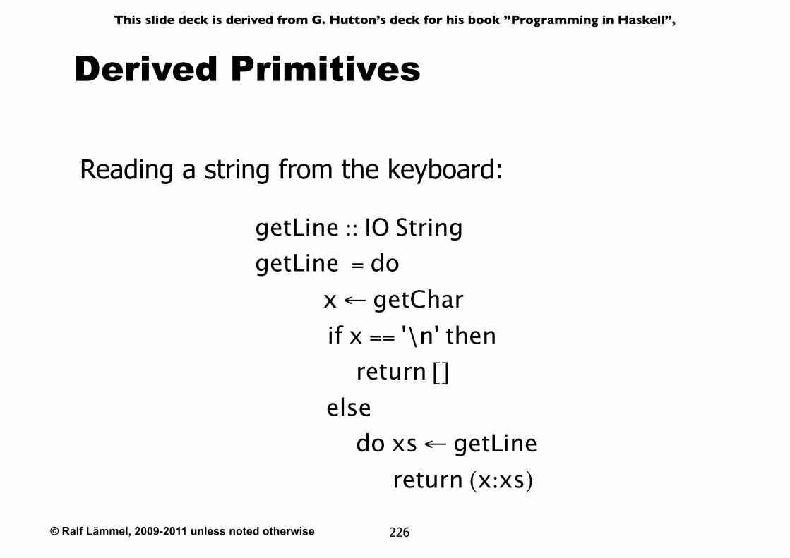
© Ralf Lämmel, 2009-2011 unless noted otherwise
This slide deck is derived from G. Hutton’s deck for his book ”Programming in Haskell”,
226
Derived Primitives
getLine :: IO StringgetLine = do
x ← getChar if x == '\n' then
return []
else do xs ← getLine
return (x:xs)
Reading a string from the keyboard:
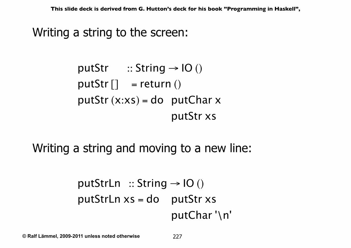
© Ralf Lämmel, 2009-2011 unless noted otherwise
This slide deck is derived from G. Hutton’s deck for his book ”Programming in Haskell”,
227
putStr :: String → IO ()
putStr [] = return ()
putStr (x:xs) = do putChar x putStr xs
Writing a string to the screen:
Writing a string and moving to a new line:
putStrLn :: String → IO ()
putStrLn xs = do putStr xs putChar '\n'
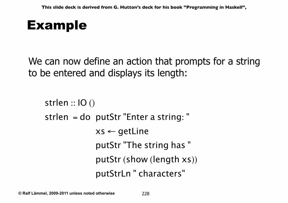
© Ralf Lämmel, 2009-2011 unless noted otherwise
This slide deck is derived from G. Hutton’s deck for his book ”Programming in Haskell”,
228
Example
We can now define an action that prompts for a string to be entered and displays its length:
strlen :: IO ()
strlen = do putStr "Enter a string: " xs ← getLine putStr "The string has " putStr (show (length xs))
putStrLn " characters"
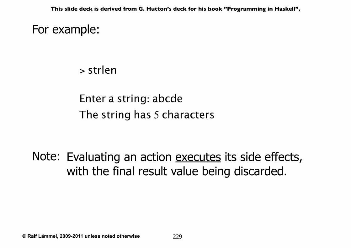
© Ralf Lämmel, 2009-2011 unless noted otherwise
This slide deck is derived from G. Hutton’s deck for his book ”Programming in Haskell”,
229
For example:
> strlen
Enter a string: abcdeThe string has 5 characters
Evaluating an action executes its side effects, with the final result value being discarded.
Note:
© Ralf Lämmel, 2009-2011 unless noted otherwise
This slide deck is derived from G. Hutton’s deck for his book ”Programming in Haskell”,
230
Hangman
Consider the following version of hangman:
๏One player secretly types in a word.
๏The other player tries to deduce the word, by entering a sequence of guesses.
๏For each guess, the computer indicates which letters in the secret word occur in the guess.
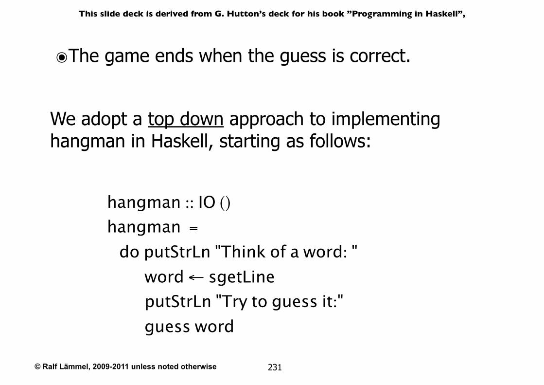
© Ralf Lämmel, 2009-2011 unless noted otherwise
This slide deck is derived from G. Hutton’s deck for his book ”Programming in Haskell”,
231
๏The game ends when the guess is correct.
hangman :: IO ()
hangman =
do putStrLn "Think of a word: " word ← sgetLine putStrLn "Try to guess it:" guess word
We adopt a top down approach to implementing hangman in Haskell, starting as follows:
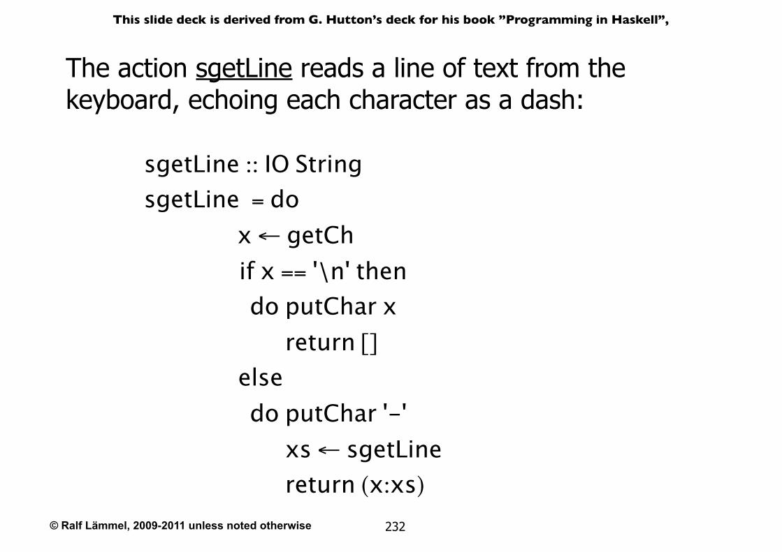
© Ralf Lämmel, 2009-2011 unless noted otherwise
This slide deck is derived from G. Hutton’s deck for his book ”Programming in Haskell”,
232
The action sgetLine reads a line of text from the keyboard, echoing each character as a dash:
sgetLine :: IO StringsgetLine = do
x ← getCh if x == '\n' then
do putChar x return []
else do putChar '-' xs ← sgetLine return (x:xs)
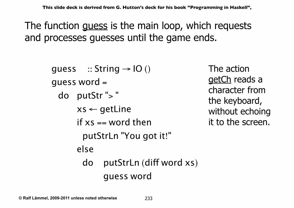
© Ralf Lämmel, 2009-2011 unless noted otherwise
This slide deck is derived from G. Hutton’s deck for his book ”Programming in Haskell”,
233
The function guess is the main loop, which requests and processes guesses until the game ends.
guess :: String → IO ()
guess word =
do putStr "> " xs ← getLine if xs == word then putStrLn "You got it!" else do putStrLn (diff word xs)
guess word
The action getCh reads a character from the keyboard, without echoing it to the screen.
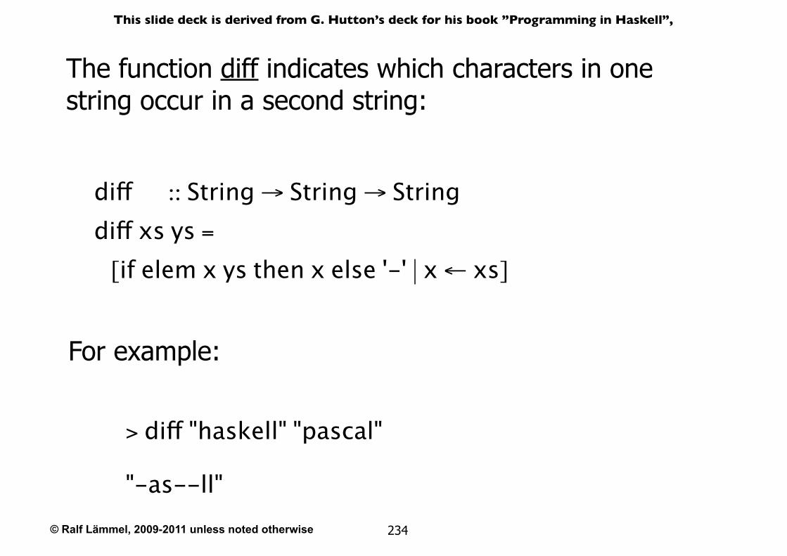
© Ralf Lämmel, 2009-2011 unless noted otherwise
This slide deck is derived from G. Hutton’s deck for his book ”Programming in Haskell”,
234
The function diff indicates which characters in one string occur in a second string:
For example:
> diff "haskell" "pascal" "-as--ll"
diff :: String → String → Stringdiff xs ys =
[if elem x ys then x else '-' | x ← xs]
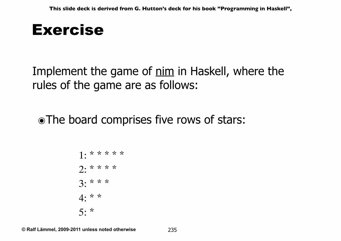
© Ralf Lämmel, 2009-2011 unless noted otherwise
This slide deck is derived from G. Hutton’s deck for his book ”Programming in Haskell”,
235
Exercise
Implement the game of nim in Haskell, where the rules of the game are as follows:
๏The board comprises five rows of stars:
1: * * * * *2: * * * *3: * * *4: * *5: *
© Ralf Lämmel, 2009-2011 unless noted otherwise
This slide deck is derived from G. Hutton’s deck for his book ”Programming in Haskell”,
236
๏Two players take it turn about to remove one or more stars from the end of a single row.
๏The winner is the player who removes the last star or stars from the board.
Hint:
Represent the board as a list of five integers that give the number of stars remaining on each row. For example, the initial board is [5,4,3,2,1].
© Ralf Lämmel, 2009-2011 unless noted otherwise
This slide deck is derived from G. Hutton’s deck for his book ”Programming in Haskell”,
237
The Countdown Problem
© Ralf Lämmel, 2009-2011 unless noted otherwise
This slide deck is derived from G. Hutton’s deck for his book ”Programming in Haskell”,
238
What Is Countdown?
๏A popular quiz programme on British television that has been running since 1982.
๏Based upon an original French version called "Des Chiffres et Des Lettres".
๏Includes a numbers game that we shall refer to as the countdown problem.
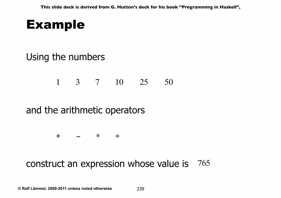
© Ralf Lämmel, 2009-2011 unless noted otherwise
This slide deck is derived from G. Hutton’s deck for his book ”Programming in Haskell”,
239
Example
1 3 7 10 25 50
Using the numbers
and the arithmetic operators
765
+ - ∗ ÷
construct an expression whose value is
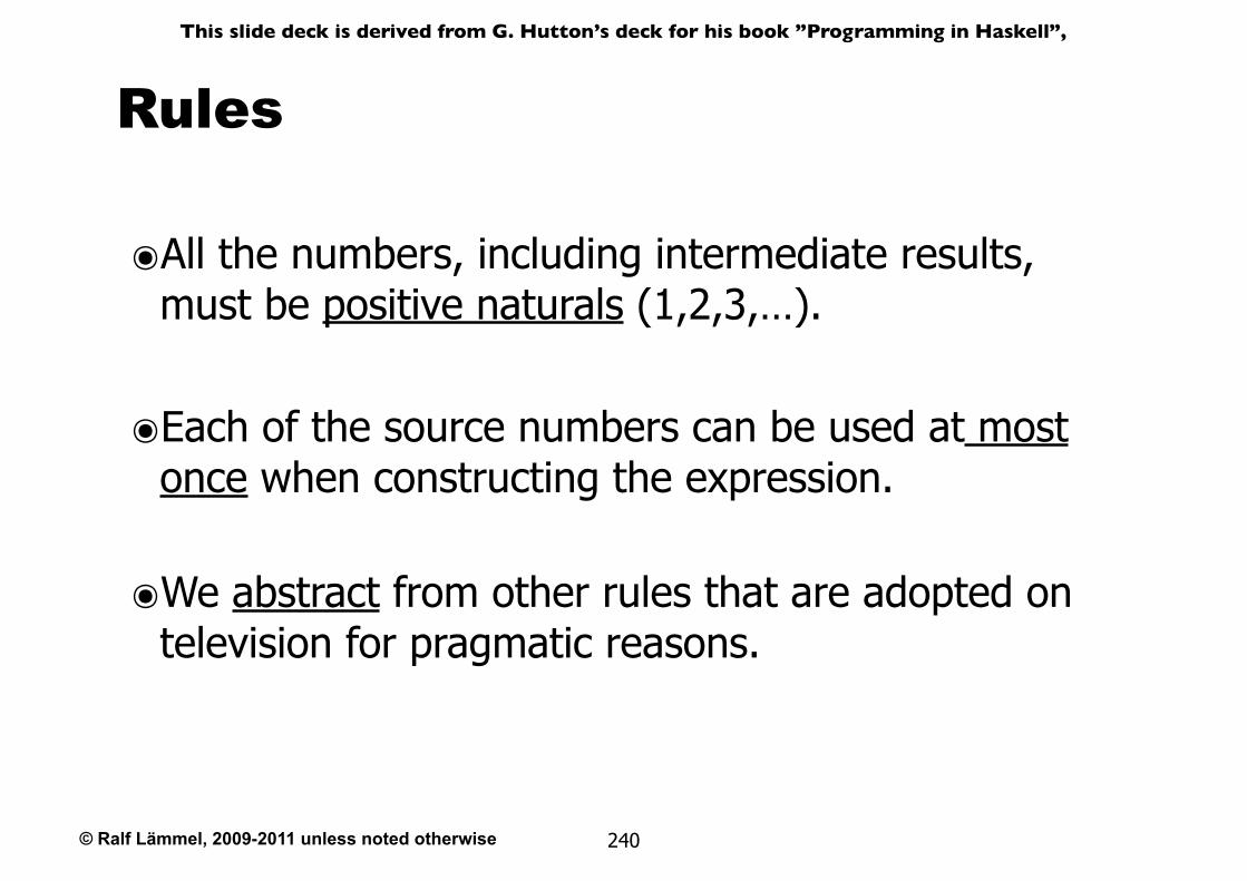
© Ralf Lämmel, 2009-2011 unless noted otherwise
This slide deck is derived from G. Hutton’s deck for his book ”Programming in Haskell”,
240
Rules
๏All the numbers, including intermediate results, must be positive naturals (1,2,3,…).
๏Each of the source numbers can be used at most once when constructing the expression.
๏We abstract from other rules that are adopted on television for pragmatic reasons.
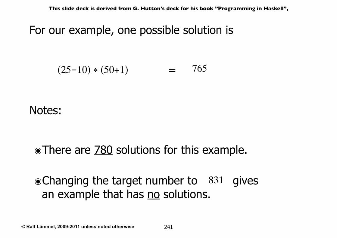
© Ralf Lämmel, 2009-2011 unless noted otherwise
This slide deck is derived from G. Hutton’s deck for his book ”Programming in Haskell”,
241
For our example, one possible solution is
๏There are 780 solutions for this example.
๏Changing the target number to gives an example that has no solutions.
Notes:
831
(25-10) ∗ (50+1) 765=
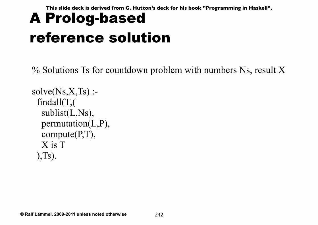
© Ralf Lämmel, 2009-2011 unless noted otherwise
This slide deck is derived from G. Hutton’s deck for his book ”Programming in Haskell”,
A Prolog-basedreference solution
242
% Solutions Ts for countdown problem with numbers Ns, result X
solve(Ns,X,Ts) :- findall(T,( sublist(L,Ns), permutation(L,P), compute(P,T), X is T ),Ts).
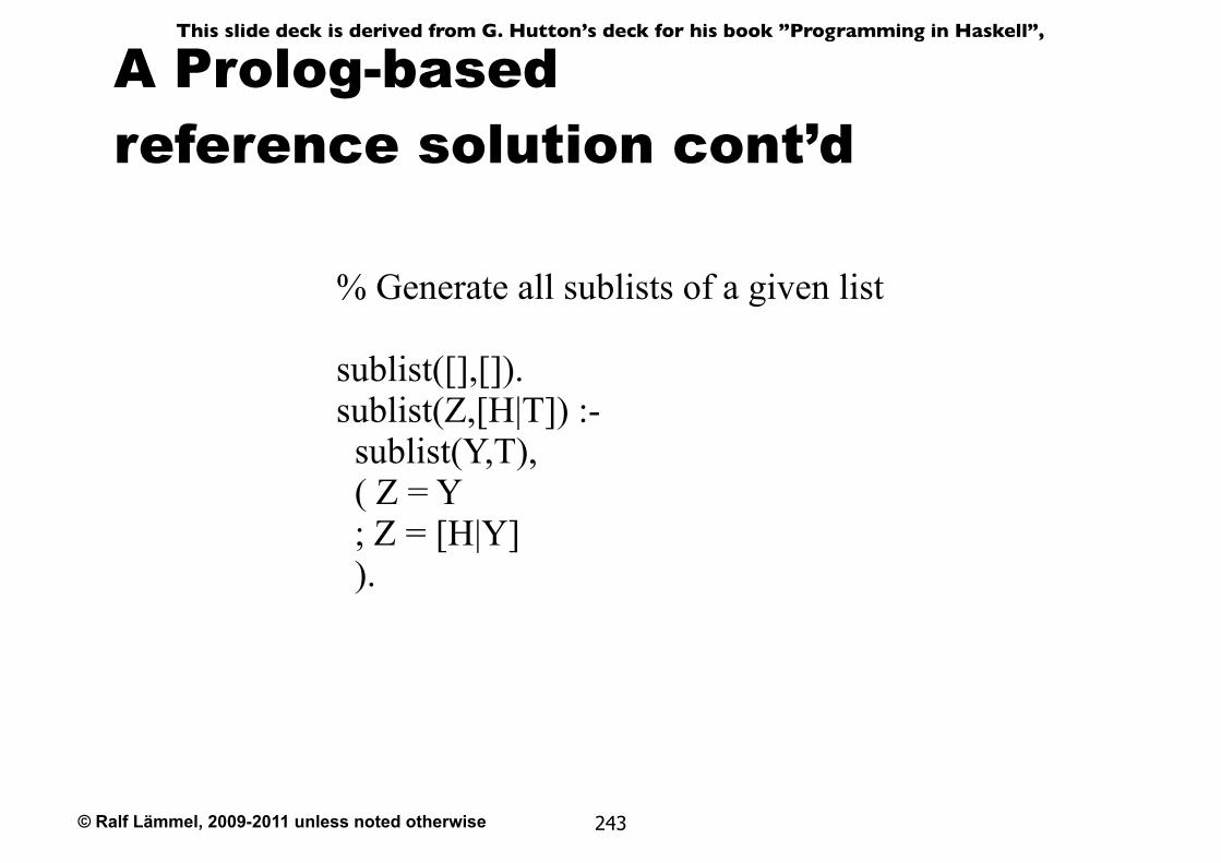
© Ralf Lämmel, 2009-2011 unless noted otherwise
This slide deck is derived from G. Hutton’s deck for his book ”Programming in Haskell”,
A Prolog-basedreference solution cont’d
243
% Generate all sublists of a given list
sublist([],[]).sublist(Z,[H|T]) :- sublist(Y,T), ( Z = Y ; Z = [H|Y] ).
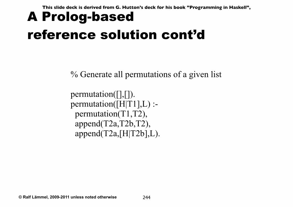
© Ralf Lämmel, 2009-2011 unless noted otherwise
This slide deck is derived from G. Hutton’s deck for his book ”Programming in Haskell”,
A Prolog-basedreference solution cont’d
244
% Generate all permutations of a given list
permutation([],[]).permutation([H|T1],L) :- permutation(T1,T2), append(T2a,T2b,T2), append(T2a,[H|T2b],L).
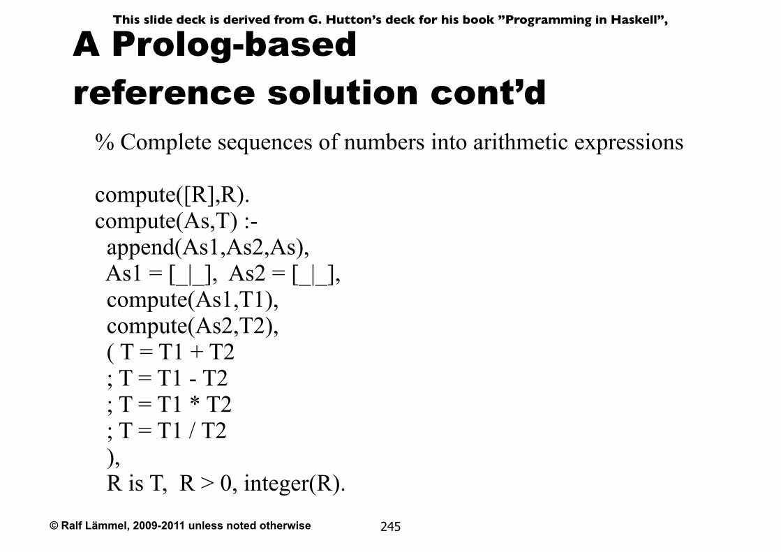
© Ralf Lämmel, 2009-2011 unless noted otherwise
This slide deck is derived from G. Hutton’s deck for his book ”Programming in Haskell”,
A Prolog-basedreference solution cont’d
245
% Complete sequences of numbers into arithmetic expressions
compute([R],R).compute(As,T) :- append(As1,As2,As), As1 = [_|_], As2 = [_|_], compute(As1,T1), compute(As2,T2), ( T = T1 + T2 ; T = T1 - T2 ; T = T1 * T2 ; T = T1 / T2 ), R is T, R > 0, integer(R).
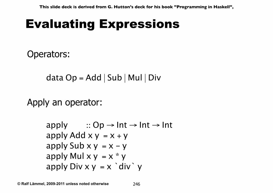
© Ralf Lämmel, 2009-2011 unless noted otherwise
This slide deck is derived from G. Hutton’s deck for his book ”Programming in Haskell”,
246
Evaluating Expressions
Operators:
data Op = Add | Sub | Mul | Div
Apply an operator:
apply :: Op → Int → Int → Intapply Add x y = x + yapply Sub x y = x - yapply Mul x y = x * yapply Div x y = x `div` y
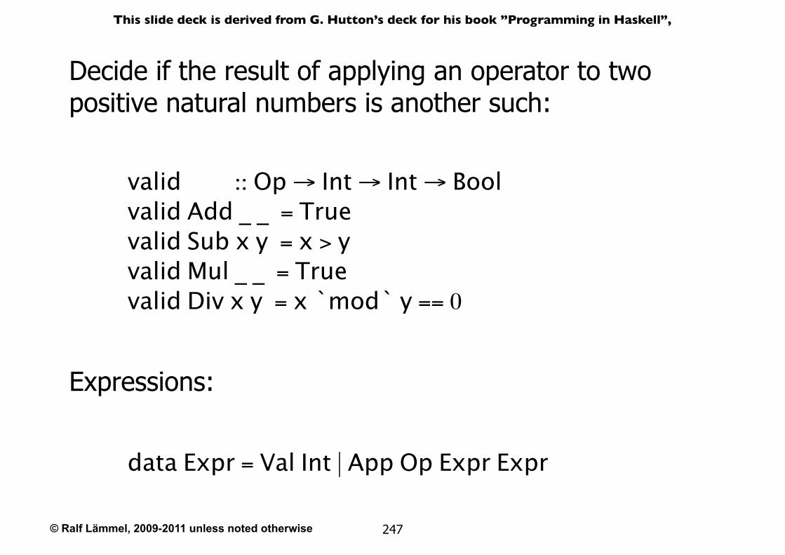
© Ralf Lämmel, 2009-2011 unless noted otherwise
This slide deck is derived from G. Hutton’s deck for his book ”Programming in Haskell”,
247
Decide if the result of applying an operator to two positive natural numbers is another such:
valid :: Op → Int → Int → Boolvalid Add _ _ = Truevalid Sub x y = x > yvalid Mul _ _ = Truevalid Div x y = x `mod` y == 0
Expressions:
data Expr = Val Int | App Op Expr Expr
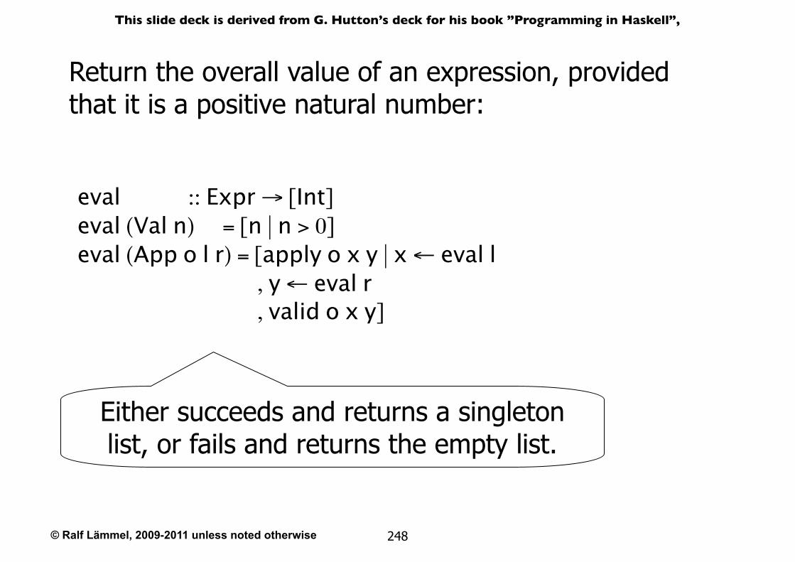
© Ralf Lämmel, 2009-2011 unless noted otherwise
This slide deck is derived from G. Hutton’s deck for his book ”Programming in Haskell”,
248
eval :: Expr → [Int]eval (Val n) = [n | n > 0]eval (App o l r) = [apply o x y | x ← eval l , y ← eval r , valid o x y]
Return the overall value of an expression, provided that it is a positive natural number:
Either succeeds and returns a singleton list, or fails and returns the empty list.
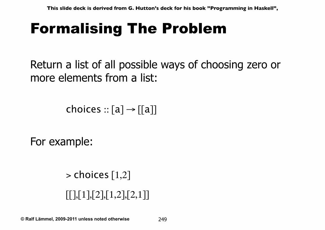
© Ralf Lämmel, 2009-2011 unless noted otherwise
This slide deck is derived from G. Hutton’s deck for his book ”Programming in Haskell”,
249
Formalising The Problem
Return a list of all possible ways of choosing zero or more elements from a list:
choices :: [a] → [[a]]
For example:
> choices [1,2]
[[],[1],[2],[1,2],[2,1]]
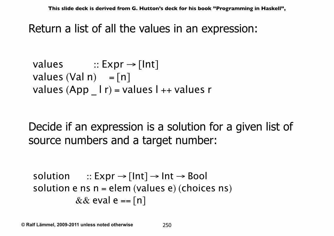
© Ralf Lämmel, 2009-2011 unless noted otherwise
This slide deck is derived from G. Hutton’s deck for his book ”Programming in Haskell”,
250
Return a list of all the values in an expression:
values :: Expr → [Int]values (Val n) = [n]values (App _ l r) = values l ++ values r
Decide if an expression is a solution for a given list of source numbers and a target number:
solution :: Expr → [Int] → Int → Boolsolution e ns n = elem (values e) (choices ns) && eval e == [n]
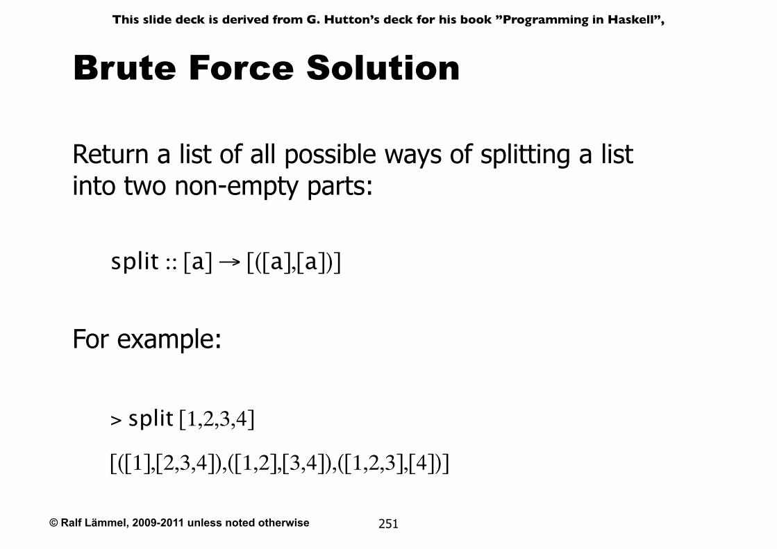
© Ralf Lämmel, 2009-2011 unless noted otherwise
This slide deck is derived from G. Hutton’s deck for his book ”Programming in Haskell”,
251
Brute Force Solution
Return a list of all possible ways of splitting a list into two non-empty parts:
split :: [a] → [([a],[a])]
For example:
> split [1,2,3,4]
[([1],[2,3,4]),([1,2],[3,4]),([1,2,3],[4])]
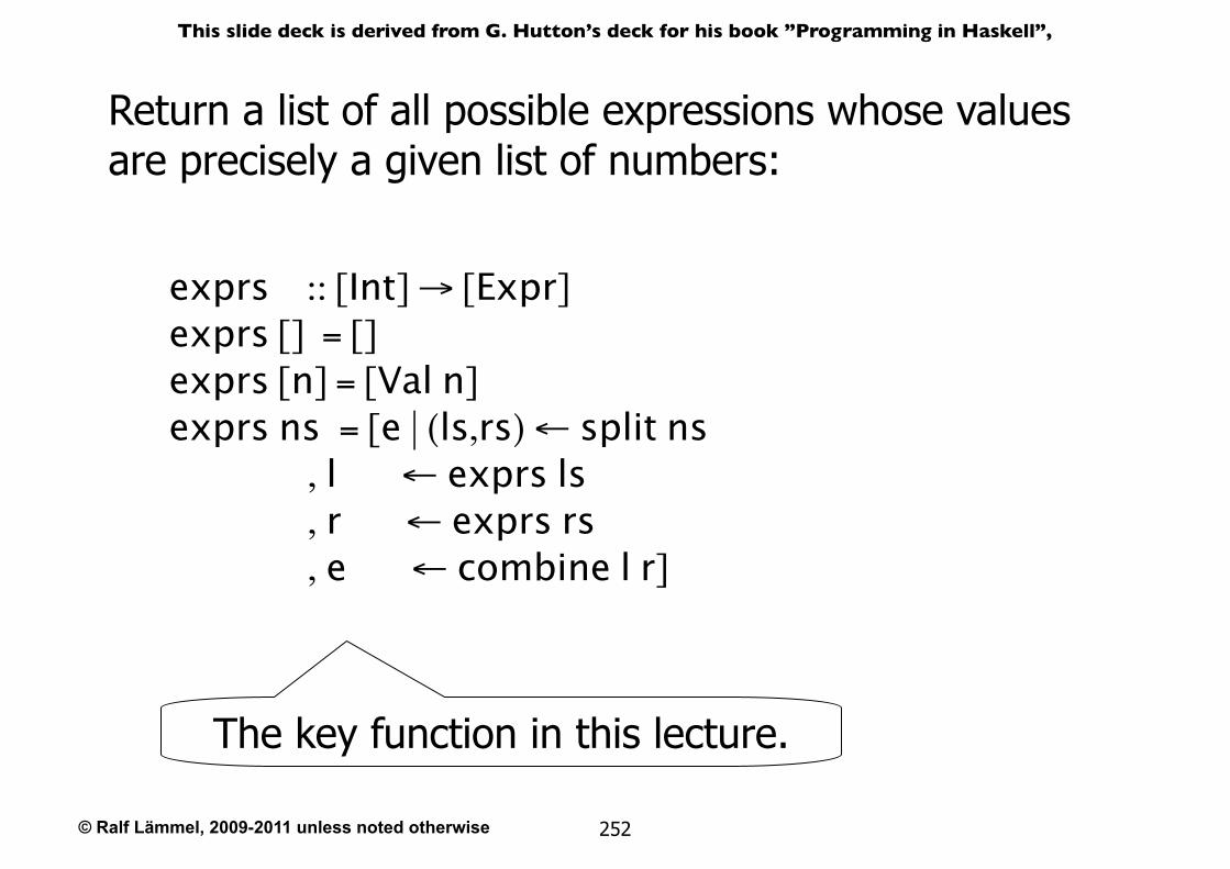
© Ralf Lämmel, 2009-2011 unless noted otherwise
This slide deck is derived from G. Hutton’s deck for his book ”Programming in Haskell”,
252
Return a list of all possible expressions whose values are precisely a given list of numbers:
exprs :: [Int] → [Expr]exprs [] = []exprs [n] = [Val n]exprs ns = [e | (ls,rs) ← split ns , l ← exprs ls , r ← exprs rs , e ← combine l r]
The key function in this lecture.
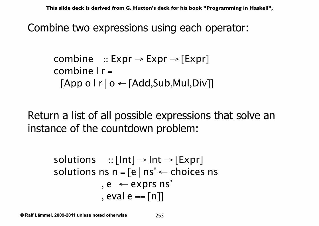
© Ralf Lämmel, 2009-2011 unless noted otherwise
This slide deck is derived from G. Hutton’s deck for his book ”Programming in Haskell”,
253
combine :: Expr → Expr → [Expr]combine l r = [App o l r | o ← [Add,Sub,Mul,Div]]
Combine two expressions using each operator:
solutions :: [Int] → Int → [Expr]solutions ns n = [e | ns' ← choices ns , e ← exprs ns' , eval e == [n]]
Return a list of all possible expressions that solve an instance of the countdown problem:
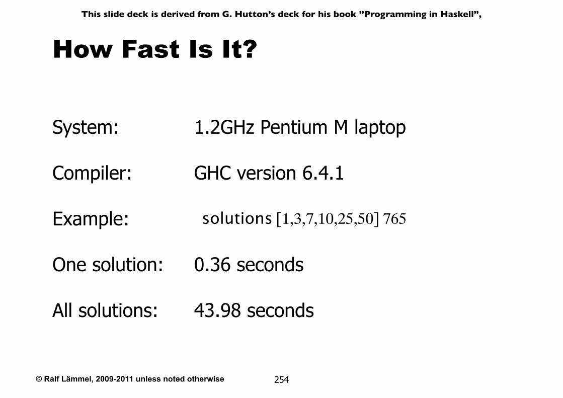
© Ralf Lämmel, 2009-2011 unless noted otherwise
This slide deck is derived from G. Hutton’s deck for his book ”Programming in Haskell”,
254
How Fast Is It?
System:
Compiler:
Example:
One solution:
All solutions:
solutions [1,3,7,10,25,50] 765
1.2GHz Pentium M laptop
GHC version 6.4.1
0.36 seconds
43.98 seconds
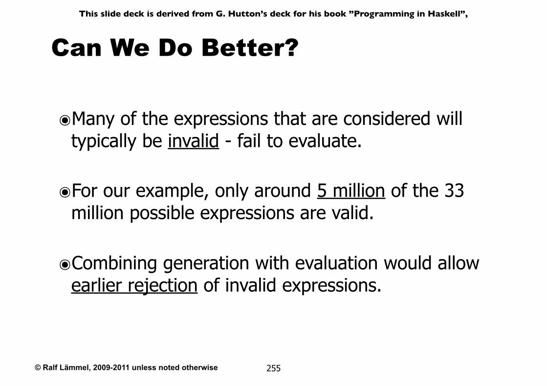
© Ralf Lämmel, 2009-2011 unless noted otherwise
This slide deck is derived from G. Hutton’s deck for his book ”Programming in Haskell”,
255
๏Many of the expressions that are considered will typically be invalid - fail to evaluate.
๏For our example, only around 5 million of the 33 million possible expressions are valid.
๏Combining generation with evaluation would allow earlier rejection of invalid expressions.
Can We Do Better?
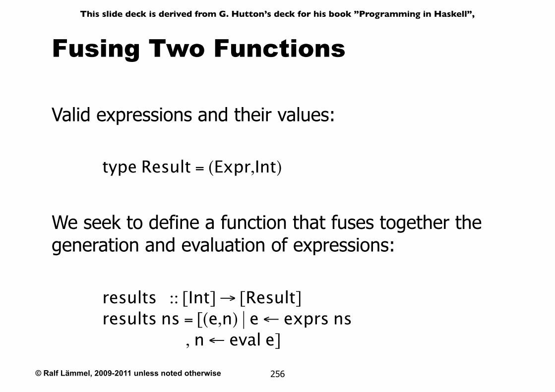
© Ralf Lämmel, 2009-2011 unless noted otherwise
This slide deck is derived from G. Hutton’s deck for his book ”Programming in Haskell”,
256
results :: [Int] → [Result]results ns = [(e,n) | e ← exprs ns , n ← eval e]
type Result = (Expr,Int)
Valid expressions and their values:
We seek to define a function that fuses together the generation and evaluation of expressions:
Fusing Two Functions
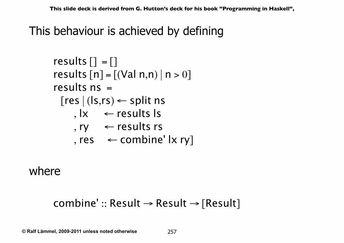
© Ralf Lämmel, 2009-2011 unless noted otherwise
This slide deck is derived from G. Hutton’s deck for his book ”Programming in Haskell”,
257
results [] = []results [n] = [(Val n,n) | n > 0]results ns = [res | (ls,rs) ← split ns , lx ← results ls , ry ← results rs , res ← combine' lx ry]
This behaviour is achieved by defining
combine' :: Result → Result → [Result]
where
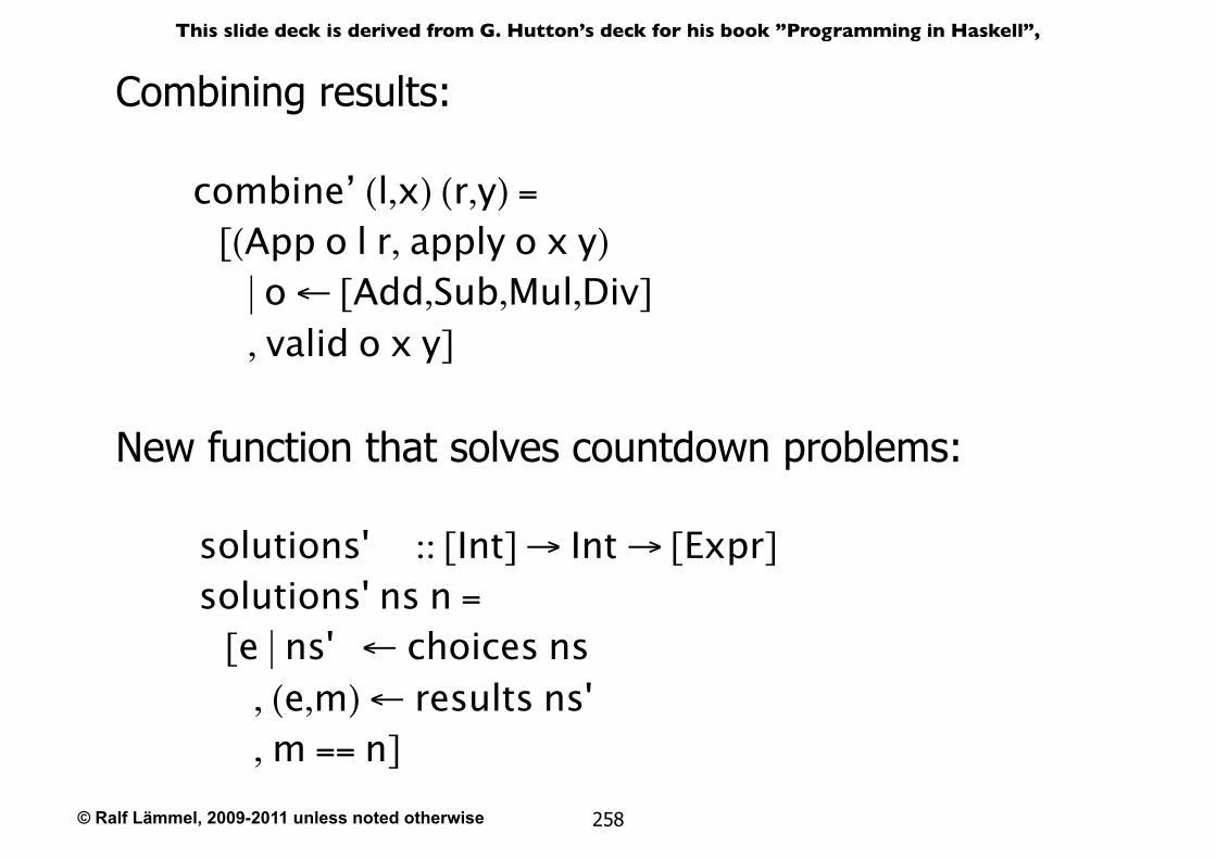
© Ralf Lämmel, 2009-2011 unless noted otherwise
This slide deck is derived from G. Hutton’s deck for his book ”Programming in Haskell”,
258
solutions' :: [Int] → Int → [Expr]solutions' ns n = [e | ns' ← choices ns , (e,m) ← results ns' , m == n]
New function that solves countdown problems:
combine’ (l,x) (r,y) = [(App o l r, apply o x y) | o ← [Add,Sub,Mul,Div]
, valid o x y]
Combining results:
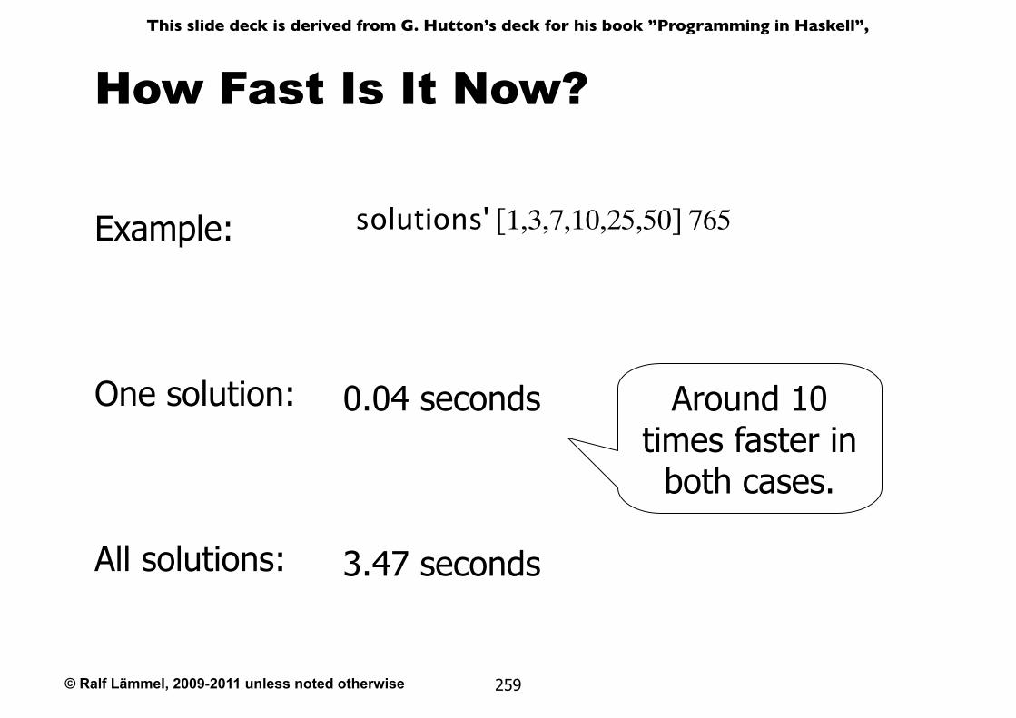
© Ralf Lämmel, 2009-2011 unless noted otherwise
This slide deck is derived from G. Hutton’s deck for his book ”Programming in Haskell”,
259
How Fast Is It Now?
Example:
One solution:
All solutions:
solutions' [1,3,7,10,25,50] 765
0.04 seconds
3.47 seconds
Around 10 times faster in
both cases.
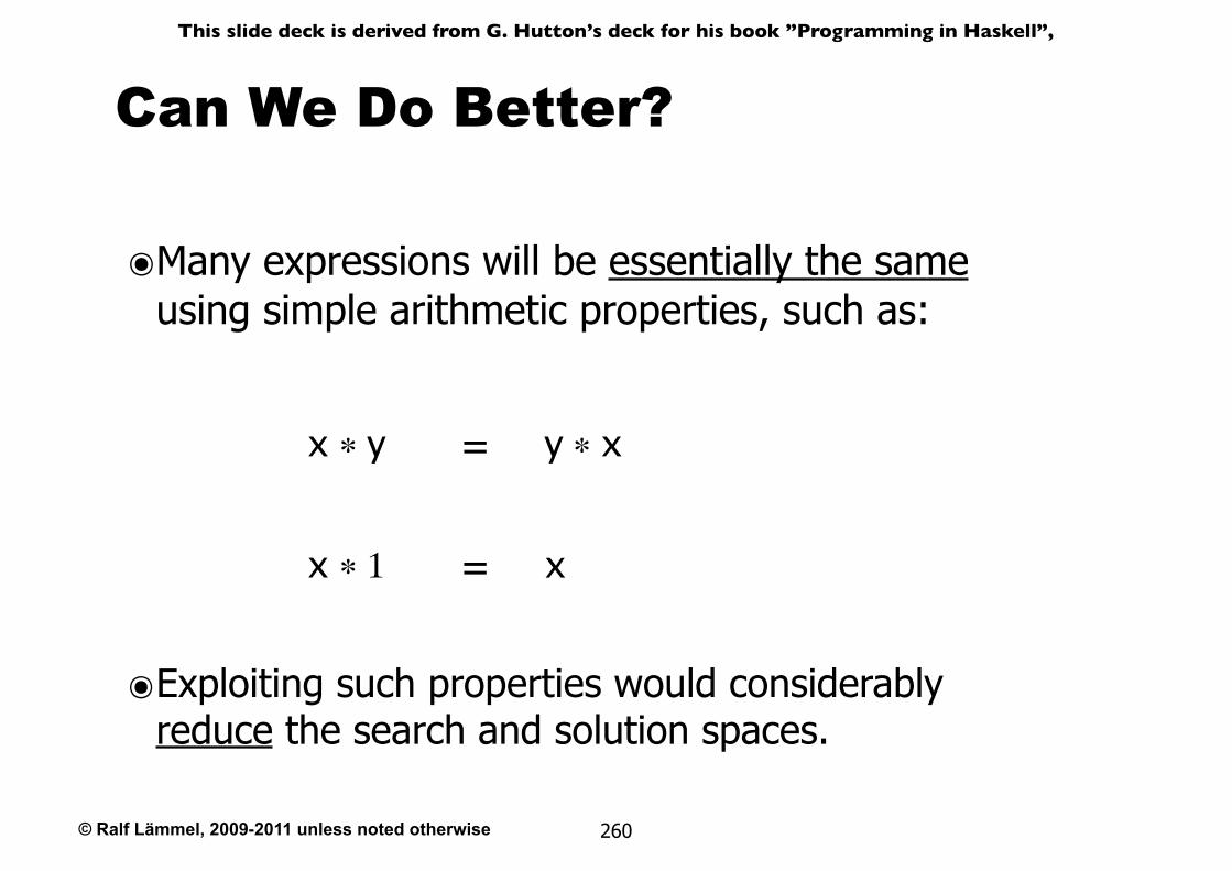
© Ralf Lämmel, 2009-2011 unless noted otherwise
This slide deck is derived from G. Hutton’s deck for his book ”Programming in Haskell”,
260
๏Many expressions will be essentially the same using simple arithmetic properties, such as:
๏Exploiting such properties would considerably reduce the search and solution spaces.
Can We Do Better?
x ∗ y y ∗ x
x ∗ 1 x
=
=
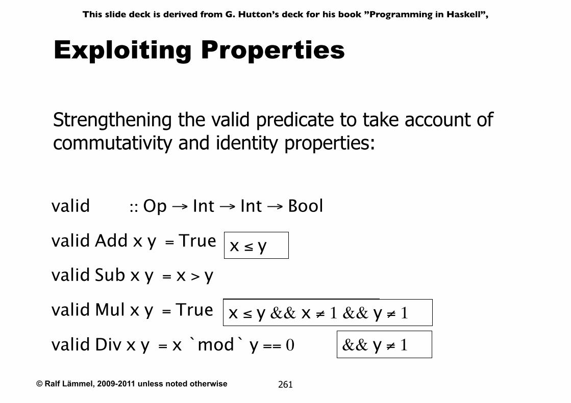
© Ralf Lämmel, 2009-2011 unless noted otherwise
This slide deck is derived from G. Hutton’s deck for his book ”Programming in Haskell”,
261
Exploiting Properties
Strengthening the valid predicate to take account of commutativity and identity properties:
valid :: Op → Int → Int → Bool
valid Add x y = True
valid Sub x y = x > y
valid Mul x y = True
valid Div x y = x `mod` y == 0
x ≤ yx ≤ y && x ≠ 1x ≤ y && x ≠ 1 && y ≠ 1
x ≤ y
&& y ≠ 1
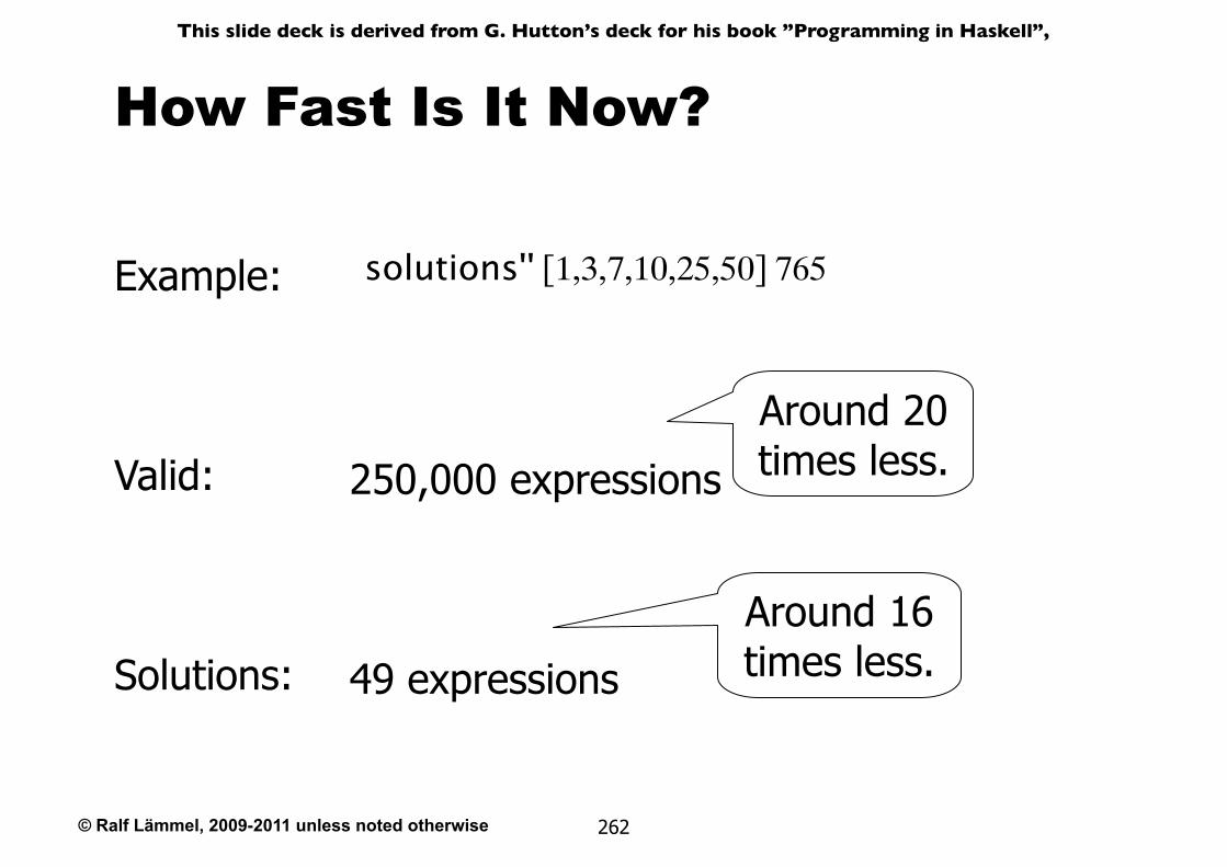
© Ralf Lämmel, 2009-2011 unless noted otherwise
This slide deck is derived from G. Hutton’s deck for his book ”Programming in Haskell”,
262
How Fast Is It Now?
Example:
Valid:
Solutions:
solutions'' [1,3,7,10,25,50] 765
250,000 expressions
49 expressions
Around 20 times less.
Around 16 times less.
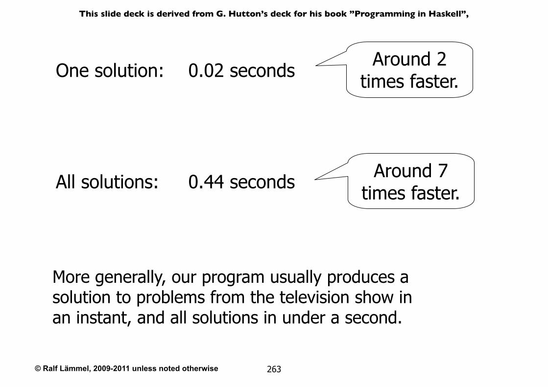
© Ralf Lämmel, 2009-2011 unless noted otherwise
This slide deck is derived from G. Hutton’s deck for his book ”Programming in Haskell”,
263
One solution:
All solutions:
0.02 seconds
0.44 seconds
Around 2 times faster.
Around 7 times faster.
More generally, our program usually produces a solution to problems from the television show in an instant, and all solutions in under a second.
© Ralf Lämmel, 2009-2011 unless noted otherwise
This slide deck is derived from G. Hutton’s deck for his book ”Programming in Haskell”,
264
End of Introduction to Haskell