Embed Size (px)
Citation preview

www.ischool.drexel.edu
INFO 631 Prof. Glenn Booker
Week 9 – Chapters 24-26
1INFO631 Week 9
www.ischool.drexel.edu
Decisions Under Risk
Ch. 24
INFO631 Week 9 2
www.ischool.drexel.edu
Decisions Under Risk
Outline
• Introducing decisions under risk
• Different techniques– Expected value decision making– Expectation variance– Monte Carlo analysis– Decision trees– Expected value of perfect information
3INFO631 Week 9
www.ischool.drexel.edu
Decisions Under Risk
• When you know the probabilities of the different outcomes and will incorporate them– Expected value decision making– Expectation variance– Monte Carlo analysis– Decision trees– Expected value of perfect information
4INFO631 Week 9

www.ischool.drexel.edu
Expected Value Decision Making
• The value of an alternative with multiple outcomes can be thought of as the average of the random individual outcomes that would occur if that alternative were repeated a large number of times– Can use PW(i), FW(i), or AE(i)
5INFO631 Week 9
www.ischool.drexel.edu
Expected Value of a Single Alternative
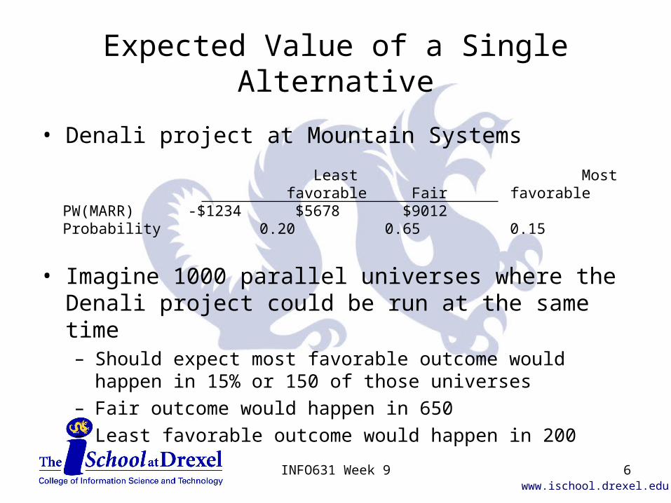
• Denali project at Mountain Systems
• Imagine 1000 parallel universes where the Denali project could be run at the same time– Should expect most favorable outcome would happen in 15% or
150 of those universes– Fair outcome would happen in 650– Least favorable outcome would happen in 200
Least Most favorable Fair favorablePW(MARR) -$1234 $5678 $9012Probability 0.20 0.65 0.15
6INFO631 Week 9
www.ischool.drexel.edu
Expected Value of a Single Alternative
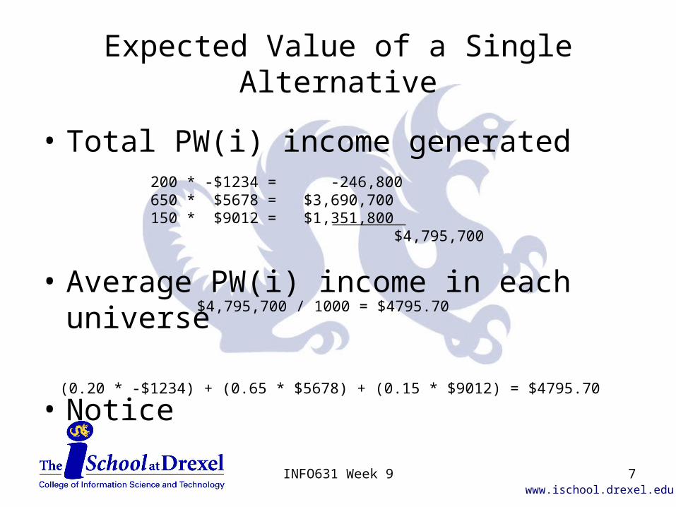
• Total PW(i) income generated
• Average PW(i) income in each universe
• Notice
200 * -$1234 = -246,800650 * $5678 = $3,690,700150 * $9012 = $1,351,800 $4,795,700
$4,795,700 / 1000 = $4795.70
(0.20 * -$1234) + (0.65 * $5678) + (0.15 * $9012) = $4795.70
7INFO631 Week 9
www.ischool.drexel.edu
Expected Value of a Single Alternative
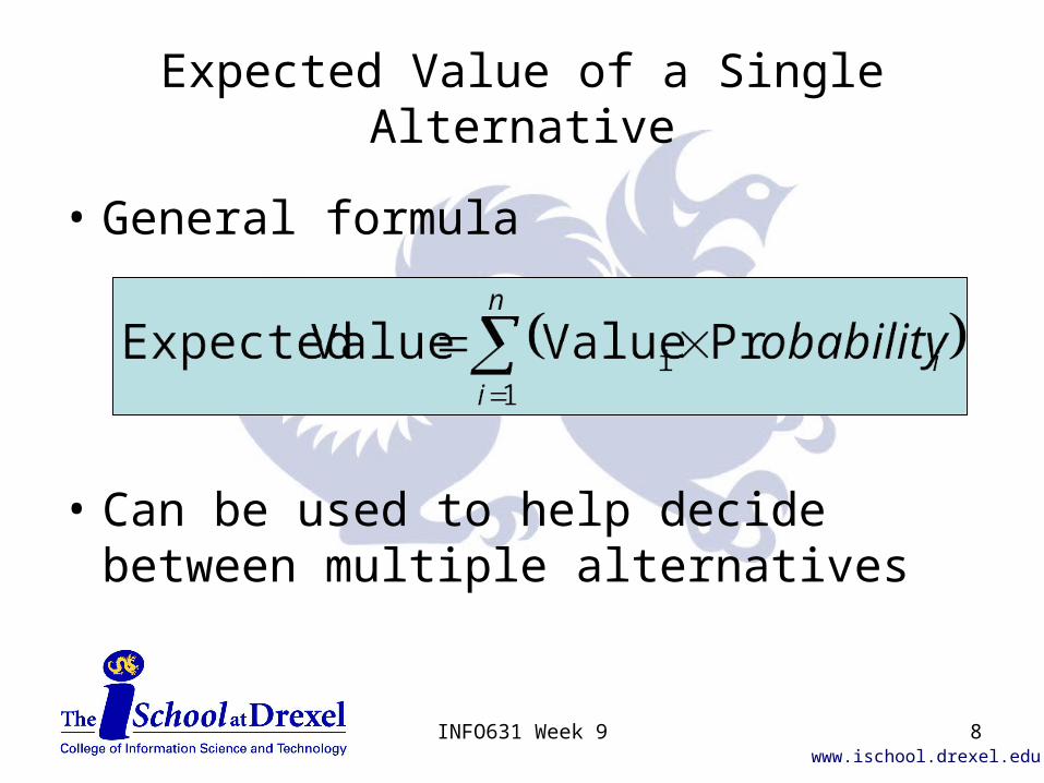
• General formula
• Can be used to help decide between multiple alternatives
8INFO631 Week 9
www.ischool.drexel.edu
Expected Value of Multiple Alternatives
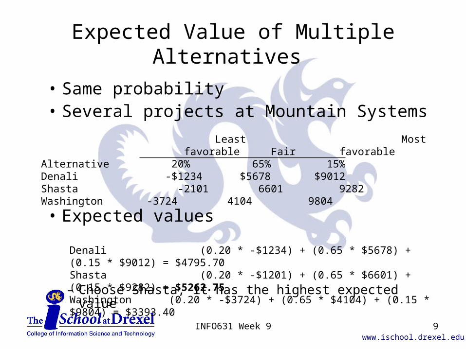
• Same probability• Several projects at Mountain Systems
• Expected values
– Choose Shasta, it has the highest expected value
Least Most favorable Fair favorableAlternative 20% 65% 15%Denali -$1234 $5678 $9012Shasta -2101 6601 9282Washington -3724 4104 9804
Denali (0.20 * -$1234) + (0.65 * $5678) + (0.15 * $9012) = $4795.70Shasta (0.20 * -$1201) + (0.65 * $6601) + (0.15 * $9282) = $5262.75Washington (0.20 * -$3724) + (0.65 * $4104) + (0.15 * $9804) = $3393.40
9INFO631 Week 9
www.ischool.drexel.edu
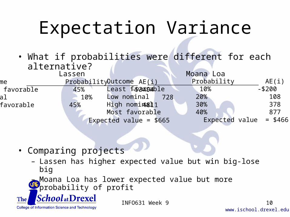
Expectation Variance
• What if probabilities were different for each alternative?
• Comparing projects– Lassen has higher expected value but win big-lose big– Moana Loa has lower expected value but more probability of
profit
Outcome Probability AE(i)Least favorable 45% -$3494Nominal 10% 728Most favorable 45% 4811
Expected value = $665
Outcome Probability AE(i)Least favorable 10% -$200Low nominal 20% 108High nominal 30% 378Most favorable 40% 877 Expected value = $466
Lassen Moana Loa
10INFO631 Week 9

www.ischool.drexel.edu
Monte Carlo Analysis
• Randomly generate combinations of input values and look at distribution of outcomes– Named after gambling resort in Monaco
• Use [a variant of] Zymurgenics project (different data)
Least favorable Fair Most favorable estimate estimate estimateInitial investment $500,000 $400,000 $360,000Operating & maintenance $1500 $1000 $800Development staff cost / month $49,000 $35,000 $24,500Development project duration 15 months 10 months 7 monthsIncome / month $24,000 $40,000 $56,000
11INFO631 Week 9
www.ischool.drexel.edu
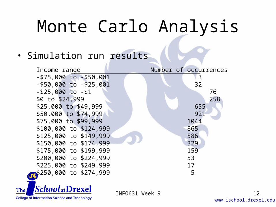
Monte Carlo Analysis
• Simulation run results
Income range Number of occurrences-$75,000 to -$50,001 3-$50,000 to -$25,001 32-$25,000 to -$1 76$0 to $24,999 258$25,000 to $49,999 655$50,000 to $74,999 921$75,000 to $99,999 1044$100,000 to $124,999 865$125,000 to $149,999 586$150,000 to $174,999 329$175,000 to $199,999 159$200,000 to $224,999 53$225,000 to $249,999 17$250,000 to $274,999 5
12INFO631 Week 9
www.ischool.drexel.edu
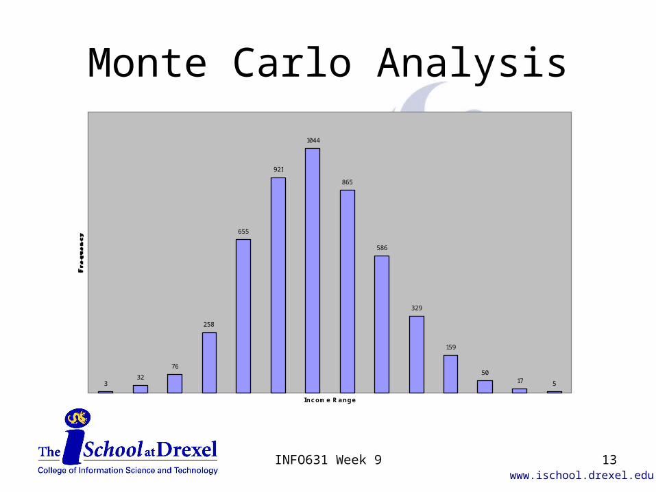
Monte Carlo Analysis
332
76
258
655
921
1044
865
586
329
159
5017 5
Income Range
13INFO631 Week 9
www.ischool.drexel.edu
Decision Trees
• Maps out possible results when there are sequences of decisions and future random events– Useful when decisions can be made in stages
• Basic Elements– Decision nodes – points in time where a decision maker makes
a decision (square)– Chance nodes – points in time where the outcome is outside the
control of the decision maker (circles)– Node sequencing
14INFO631 Week 9

www.ischool.drexel.edu
Sample Decision Tree
Do A
Do B
-$6000
-$4000
$1200/yr
$800/yr
$2848/yr
$1437/yr
$1100/yr
$1000/yr
Do D
Do C
-$5490
$835/yr
$3615/yr
$851/yr
$1526/yr
$1037/yr
$1214/yr
Period 1 2 Years
Period 2 6 Years
15INFO631 Week 9
www.ischool.drexel.edu
Decision Tree Analysis, Part 1
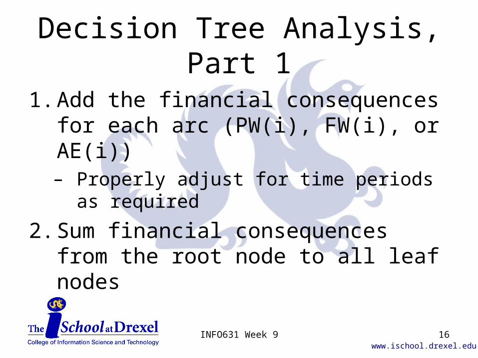
1. Add the financial consequences for each arc (PW(i), FW(i), or AE(i))– Properly adjust for time periods as required
2. Sum financial consequences from the root node to all leaf nodes
16INFO631 Week 9
www.ischool.drexel.edu
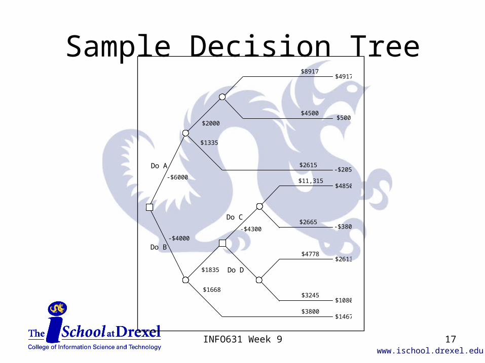
Sample Decision Tree
Do A
Do B
-$6000
-$4000
$2000
$1335
$8917
$4500
$1835
$1668
Do D
Do C
-$4300
$2615
$11,315
$2665
$4778
$3245
$3800
$4917
$500
-$2050
$4850
-$3800
$2613
$1080
$1467
17INFO631 Week 9
www.ischool.drexel.edu
Decision Tree Analysis, Part 2
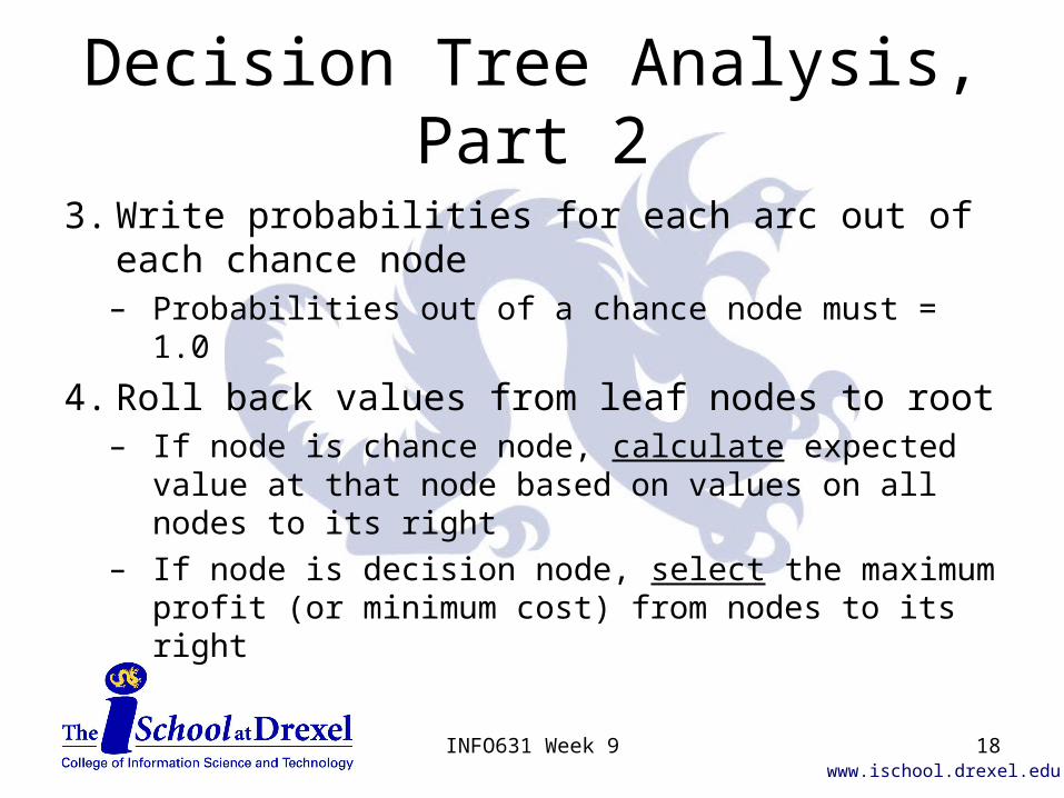
3. Write probabilities for each arc out of each chance node– Probabilities out of a chance node must = 1.0
4. Roll back values from leaf nodes to root– If node is chance node, calculate expected
value at that node based on values on all nodes to its right
– If node is decision node, select the maximum profit (or minimum cost) from nodes to its right
18INFO631 Week 9

www.ischool.drexel.edu
Sample Decision Tree
Do A
Do B
$1200
$3150
$1800
Do D
Do C
$2000
$1390
$4917
$500
-$2050
$4850
-$3800
$2613
$1080
$1467
3/5
2/5
5/8
3/8
3/5
2/5
2/5
3/55/8
3/8$2000
$1800
19INFO631 Week 9
www.ischool.drexel.edu
Expected Value of Perfect Information
• Value at root node is expected value of decision tree based on current information– Current information is known to be imperfect
• Reasonable follow-on question
– Research, experimentation, prototyping, …– Might even be able to eliminate one or more paths through the tree
because you may discover them to be impossible
• Analyzed decision tree provides information that will help answer that question
“Would there be any value in taking actions that would reducethe probability of ending up in an undesirable future state?”
20INFO631 Week 9
www.ischool.drexel.edu
Expected Value of Perfect Information
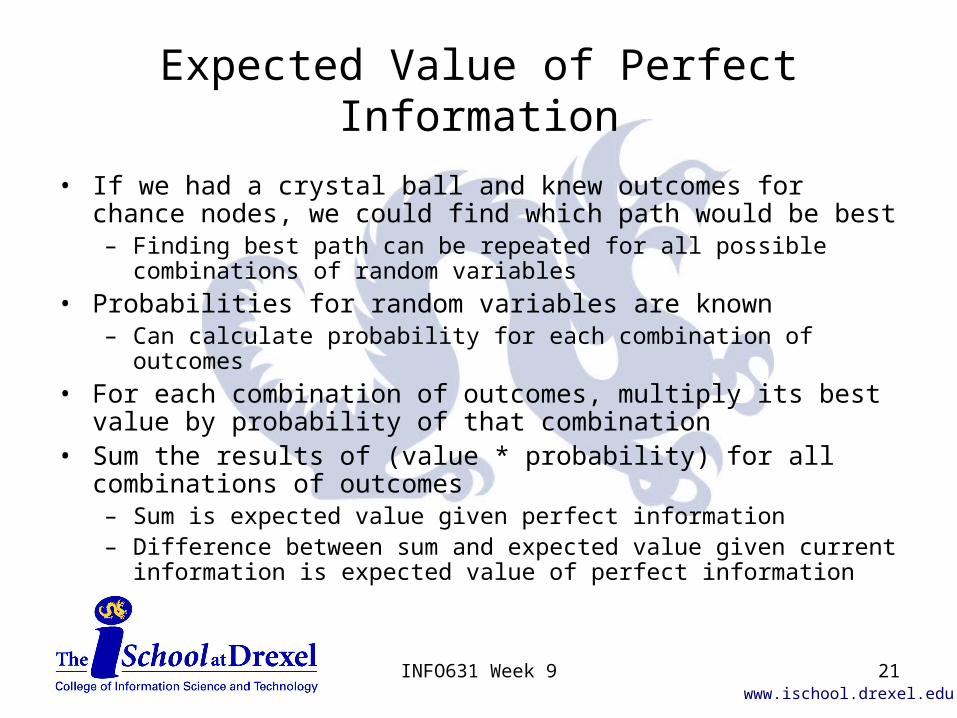
• If we had a crystal ball and knew outcomes for chance nodes, we could find which path would be best– Finding best path can be repeated for all possible combinations of
random variables
• Probabilities for random variables are known– Can calculate probability for each combination of outcomes
• For each combination of outcomes, multiply its best value by probability of that combination
• Sum the results of (value * probability) for all combinations of outcomes– Sum is expected value given perfect information– Difference between sum and expected value given current information is
expected value of perfect information
21INFO631 Week 9

www.ischool.drexel.edu
Expected Value of Perfect Information
• EVPI is upper limit on how much to spend to gain further knowledge– Probably impossible to actually get perfect
information, organization should plan on spending less
22INFO631 Week 9
www.ischool.drexel.edu
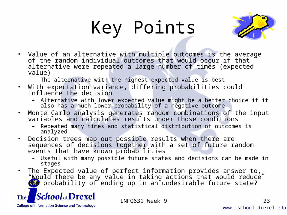
Key Points• Value of an alternative with multiple outcomes is the average of the random individual
outcomes that would occur if that alternative were repeated a large number of times (expected value)
– The alternative with the highest expected value is best• With expectation variance, differing probabilities could influence the decision
– Alternative with lower expected value might be a better choice if it also has a much lower probability of a negative outcome
• Monte Carlo analysis generates random combinations of the input variables and calculates results under those conditions
– Repeated many times and statistical distribution of outcomes is analyzed• Decision trees map out possible results when there are sequences of decisions
together with a set of future random events that have known probabilities– Useful with many possible future states and decisions can be made in stages
• The Expected value of perfect information provides answer to, “Would there be any value in taking actions that would reduce the probability of ending up in an undesirable future state?”
23INFO631 Week 9

www.ischool.drexel.edu
Decisions Under Uncertainty
Ch. 25
INFO631 Week 9
Slides adapted from Steve Tockey – Return on Software
24
www.ischool.drexel.edu
Decisions Under Uncertainty
Outline
• Introducing decisions under uncertainty
• Different Techniques– Payoff matrix– Laplace Rule– Maximin Rule– Maximax Rule– Hurwicz Rule– Minimax Regret Rule
25INFO631 Week 9
www.ischool.drexel.edu
Decisions Under Uncertainty
• Used when impossible to assign probabilities to outcomes– Can also be used when you don’t want to put probabilities on
outcomes, e.g., safety-critical software system where a failure could threaten human life
• People may not react well to an assigned probability of fatality
• If probabilities can be assigned, Decision Making under Risk should be used
26INFO631 Week 9
www.ischool.drexel.edu
Payoff Matrix
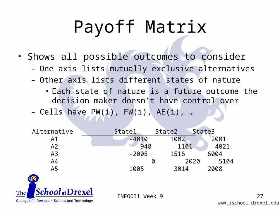
• Shows all possible outcomes to consider– One axis lists mutually exclusive alternatives– Other axis lists different states of nature
• Each state of nature is a future outcome the decision maker doesn’t have control over
– Cells have PW(i), FW(i), AE(i), …
Alternative State1 State2 State3 A1 -4010 1002 2001 A2 948 1101 4021 A3 -2005 1516 6004 A4 0 2020 5104 A5 1005 3014 2008
27INFO631 Week 9
www.ischool.drexel.edu
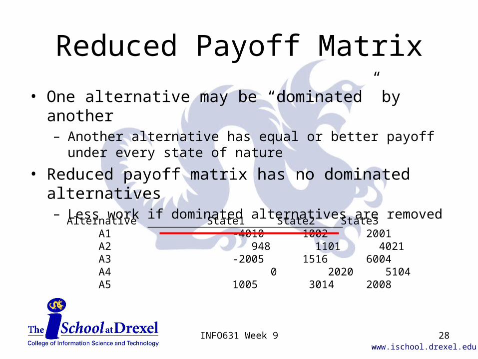
Reduced Payoff Matrix
• One alternative may be “dominated” by another– Another alternative has equal or better payoff under every state
of nature
• Reduced payoff matrix has no dominated alternatives– Less work if dominated alternatives are removed
Alternative State1 State2 State3 A1 -4010 1002 2001 A2 948 1101 4021 A3 -2005 1516 6004 A4 0 2020 5104 A5 1005 3014 2008
28INFO631 Week 9
www.ischool.drexel.edu
Laplace Rule
• Assumes each state of nature is equally likely– Sometimes called “principle of insufficient
reason”
• Calculate average payoff for each alternative across all states of nature– Same as expected value analysis for multiple
alternatives with equal probabilities
29INFO631 Week 9
www.ischool.drexel.edu
Laplace Rule
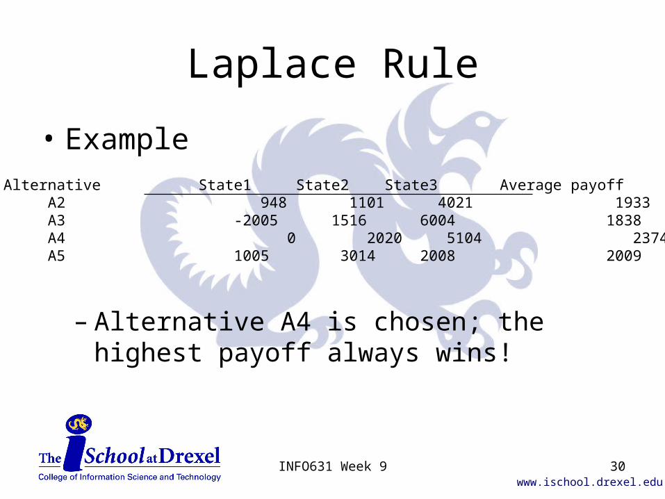
• Example
– Alternative A4 is chosen; the highest payoff always wins!
Alternative State1 State2 State3 Average payoff A2 948 1101 4021 1933 A3 -2005 1516 6004 1838 A4 0 2020 5104 2374 A5 1005 3014 2008 2009
30INFO631 Week 9
www.ischool.drexel.edu
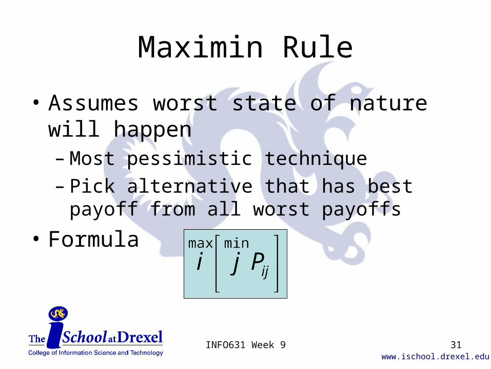
Maximin Rule
• Assumes worst state of nature will happen– Most pessimistic technique– Pick alternative that has best payoff from all
worst payoffs
• Formula
31INFO631 Week 9
www.ischool.drexel.edu
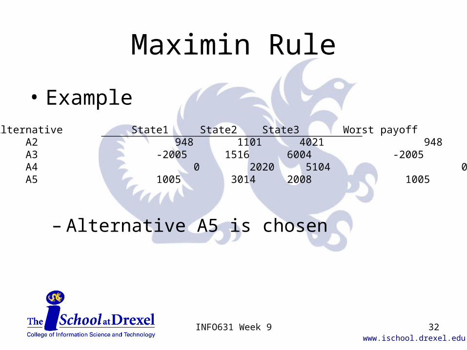
Maximin Rule
• Example
– Alternative A5 is chosen
Alternative State1 State2 State3 Worst payoff A2 948 1101 4021 948 A3 -2005 1516 6004 -2005 A4 0 2020 5104 0 A5 1005 3014 2008 1005
32INFO631 Week 9
www.ischool.drexel.edu
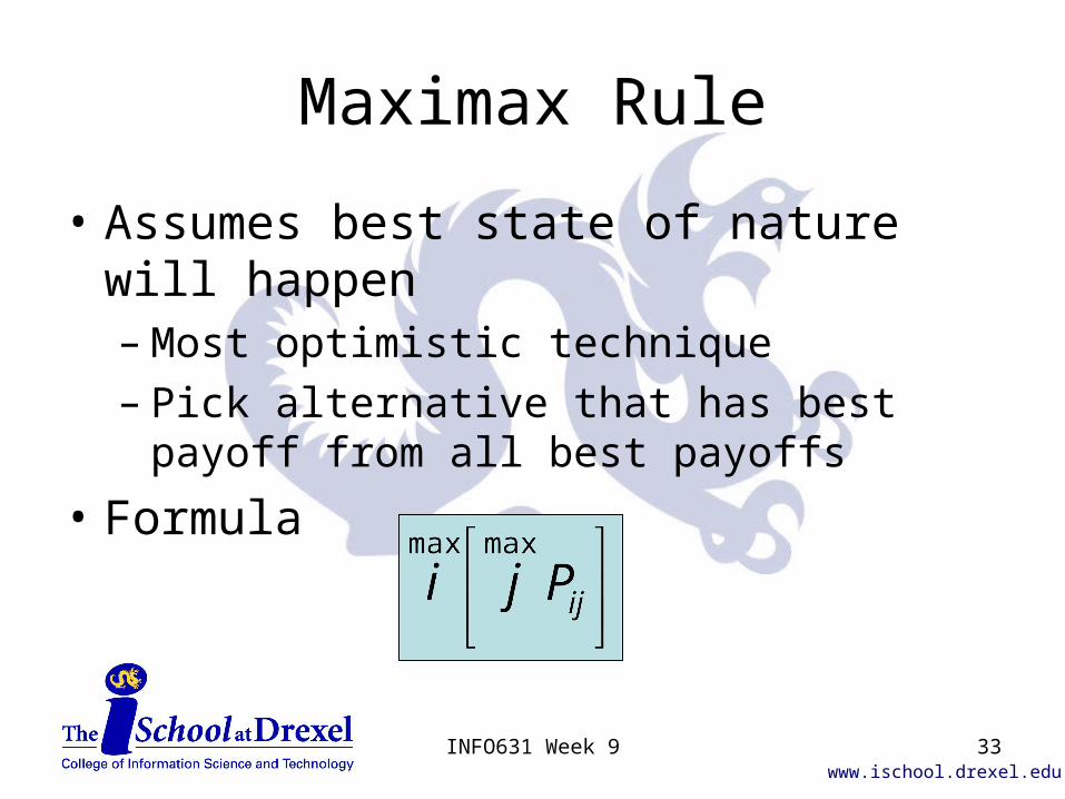
Maximax Rule
• Assumes best state of nature will happen– Most optimistic technique– Pick alternative that has best payoff from all
best payoffs
• Formula
33INFO631 Week 9
www.ischool.drexel.edu
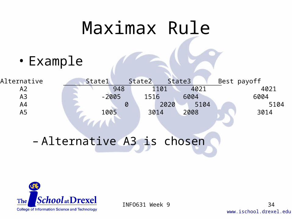
Maximax Rule
• Example
– Alternative A3 is chosen
Alternative State1 State2 State3 Best payoff A2 948 1101 4021 4021 A3 -2005 1516 6004 6004 A4 0 2020 5104 5104 A5 1005 3014 2008 3014
34INFO631 Week 9
www.ischool.drexel.edu
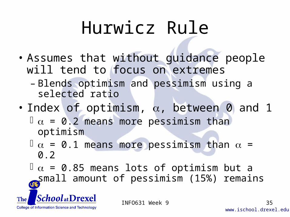
Hurwicz Rule
• Assumes that without guidance people will tend to focus on extremes– Blends optimism and pessimism using a
selected ratio
• Index of optimism, , between 0 and 1 = 0.2 means more pessimism than optimism = 0.1 means more pessimism than = 0.2 = 0.85 means lots of optimism but a small
amount of pessimism (15%) remains
35INFO631 Week 9
www.ischool.drexel.edu
Hurwicz Rule
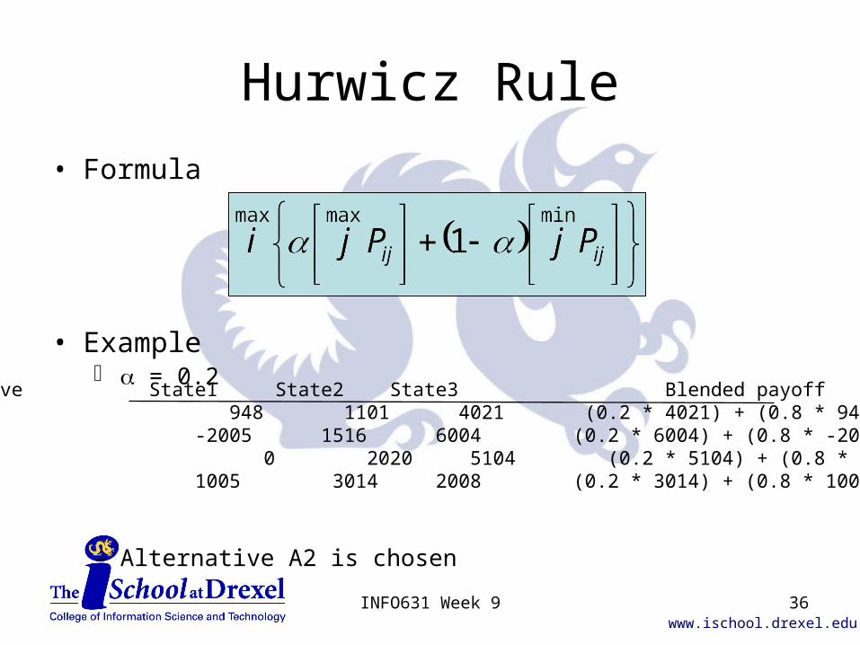
• Formula
• Example = 0.2
– Alternative A2 is chosen
Alternative State1 State2 State3 Blended payoff A2 948 1101 4021 (0.2 * 4021) + (0.8 * 948) = 1563 A3 -2005 1516 6004 (0.2 * 6004) + (0.8 * -2005) = -403 A4 0 2020 5104 (0.2 * 5104) + (0.8 * 0) = 1021 A5 1005 3014 2008 (0.2 * 3014) + (0.8 * 1005) = 1407
36INFO631 Week 9
www.ischool.drexel.edu
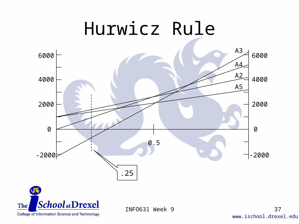
Hurwicz Rule6000
4000
2000
0
-2000
6000
4000
2000
0
-2000
0.5
A2
A3
A4
A5
.25
37INFO631 Week 9
www.ischool.drexel.edu
Minimax Regret Rule
• Minimize regret you would have if you chose wrong alternative under each state of nature– If you selected A1 and state of nature happened where A1 had
the best payoff then you would have no regrets– If you selected A1 and state of nature happened where another
alternative was better, you can quantify regret as difference between payoff you chose and best payoff under that state of nature
• Regret matrix– Need to calculate– Difference between payoff you chose and best payoff under that
state of nature
38INFO631 Week 9
www.ischool.drexel.edu
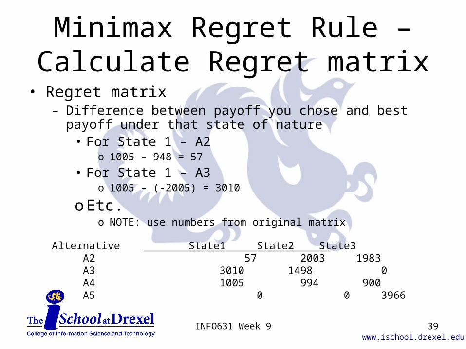
Minimax Regret Rule – Calculate Regret matrix
• Regret matrix– Difference between payoff you chose and best payoff under that
state of nature• For State 1 – A2
o 1005 – 948 = 57
• For State 1 – A3o 1005 – (-2005) = 3010
oEtc.o NOTE: use numbers from original matrix
Alternative State1 State2 State3 A2 57 2003 1983 A3 3010 1498 0 A4 1005 994 900 A5 0 0 3966
39INFO631 Week 9
www.ischool.drexel.edu
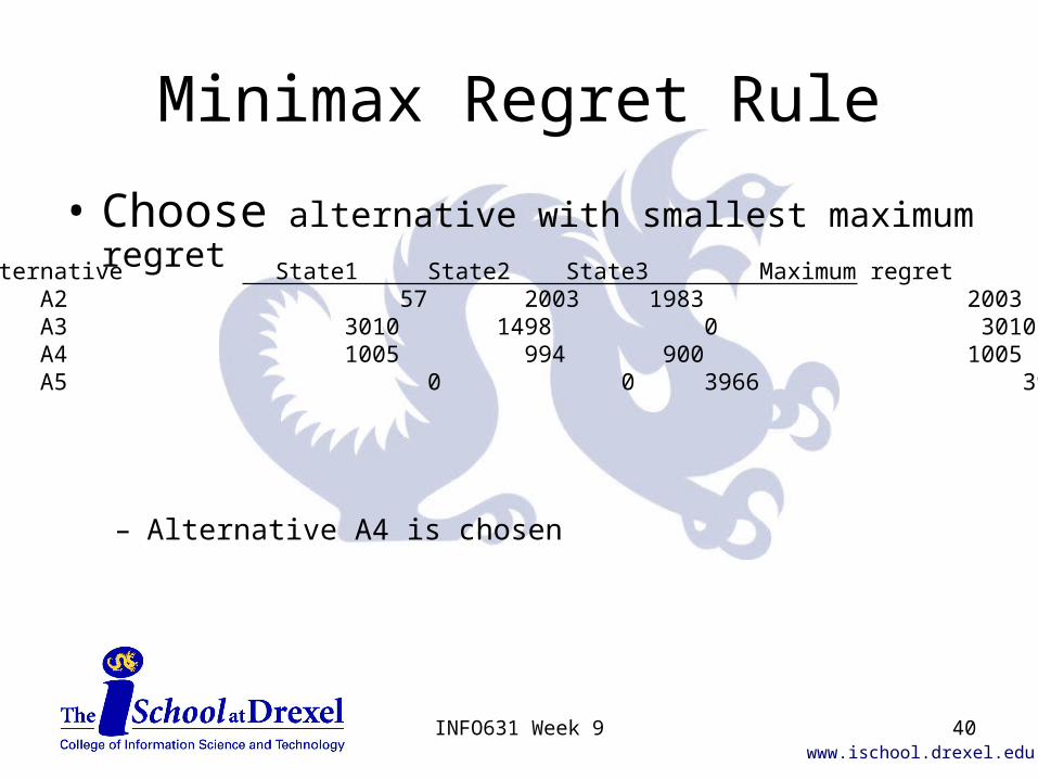
Minimax Regret Rule
• Choose alternative with smallest maximum regret
– Alternative A4 is chosen
Alternative State1 State2 State3 Maximum regret A2 57 2003 1983 2003 A3 3010 1498 0 3010 A4 1005 994 900 1005 A5 0 0 3966 3996
40INFO631 Week 9
www.ischool.drexel.edu
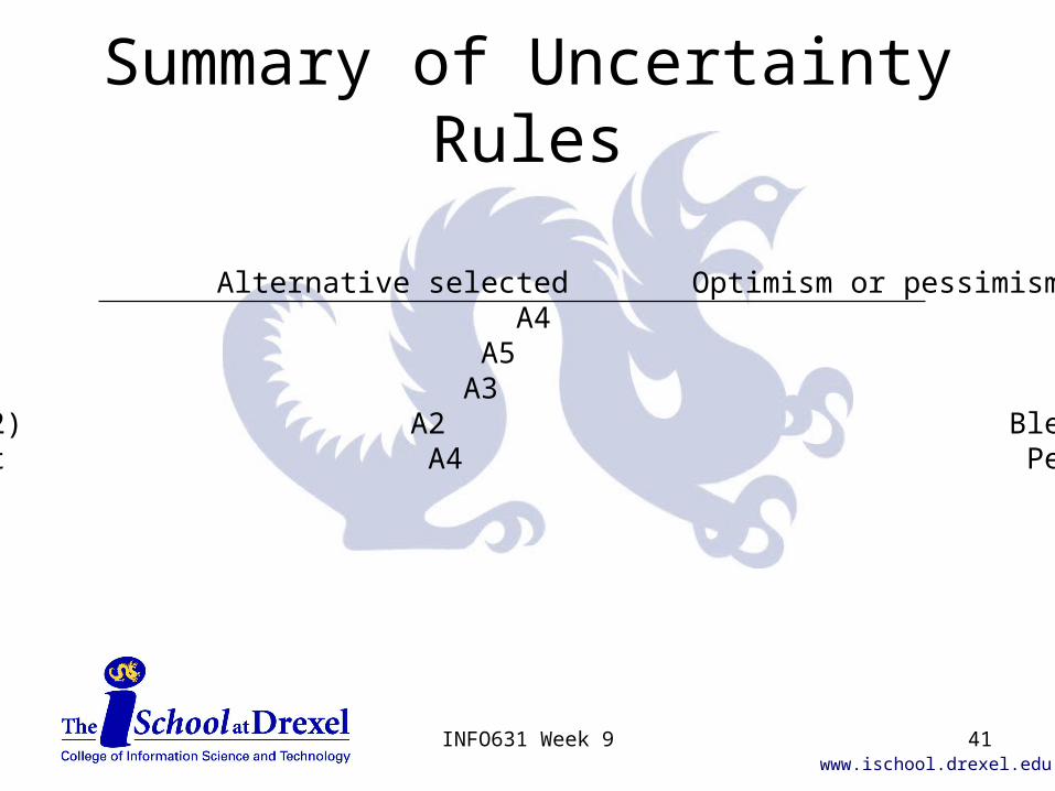
Summary of Uncertainty Rules
Decision rule Alternative selected Optimism or pessimismLaplace A4 NeitherMaximin A5 PessimismMaximax A3 OptimismHurwicz (a=0.2) A2 BlendMinimax regret A4 Pessimism
41INFO631 Week 9
www.ischool.drexel.edu
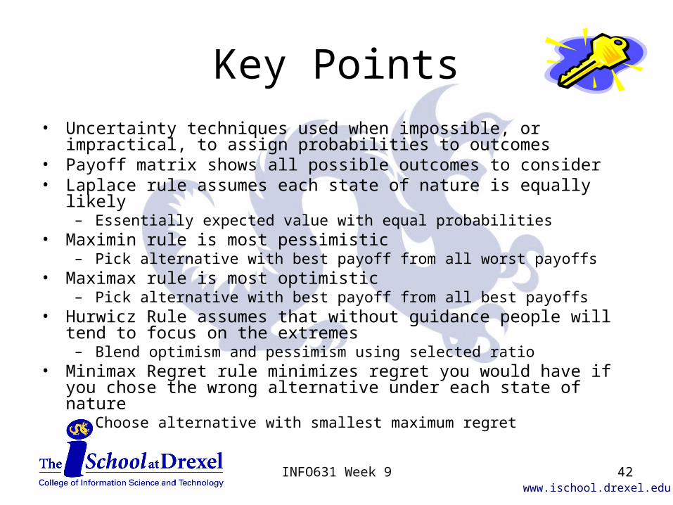
Key Points• Uncertainty techniques used when impossible, or impractical, to assign
probabilities to outcomes• Payoff matrix shows all possible outcomes to consider• Laplace rule assumes each state of nature is equally likely
– Essentially expected value with equal probabilities• Maximin rule is most pessimistic
– Pick alternative with best payoff from all worst payoffs• Maximax rule is most optimistic
– Pick alternative with best payoff from all best payoffs• Hurwicz Rule assumes that without guidance people will tend to focus on
the extremes– Blend optimism and pessimism using selected ratio
• Minimax Regret rule minimizes regret you would have if you chose the wrong alternative under each state of nature
– Choose alternative with smallest maximum regret
42INFO631 Week 9
www.ischool.drexel.edu
Multiple Attribute Decisions
Ch. 26
INFO631 Week 9 43
www.ischool.drexel.edu
Multiple Attribute Decisions
Outline
• Introducing multiple attribute decisions
• Case study: Fly-by-Night Air
• Different kinds of “value”
• Choosing attributes
• Measurement scales
• Non-compensatory techniques
• Compensatory techniques
44INFO631 Week 9
www.ischool.drexel.edu
IntroducingMultiple Attribute Decisions
• Previous chapters explained how to make decisions using a single criterion, money– Alternative with best PW(i), AE(i), incremental IRR, incremental
benefit-cost ratio, etc. is selected
• Aside from technical feasibility, money is almost always the most important decision criterion– But not the only one– Often, other criteria (“attributes”) must be considered and can’t
be cast in terms of money
45INFO631 Week 9
www.ischool.drexel.edu
Case Study: Fly-by-Night (FBN) Airlines
• 10-year old regional airline with above average growth• Moving into nationwide market as no-frills carrier• As part of strategic planning, IT department charged with
examining airline reservations systems– 10 year planning horizon, effective income tax rate=37%,
after-tax MARR=15%• Research has identified five technically-viable
alternatives – Keep existing software– Buy Jupiter commercial system– Buy Sword commercial system– Buy Guppy commercial system– Develop new software in-house– Develop new software offshore
46INFO631 Week 9
www.ischool.drexel.edu
Different Kinds of “Value”
• Decision process is all about maximizing value– Choose from available alternatives the one that
maximizes value• When value is expressed as money, decision
process may be complex but is straightforward– Money isn’t the only kind of value– Money is really only a way to quantify value
• Two kinds of value– Use-value - the ability to get things done, the
properties of the object that cause it to perform– Esteem value - the properties that make it desirable
47INFO631 Week 9
www.ischool.drexel.edu
Choosing Attributes
• Decisions should be based on appropriate attributes– Each attribute should capture a unique dimension of decision– Set of attributes should cover important aspects of decision– Differences in attribute values should be meaningful in
distinguishing among alternatives– Each attribute should distinguish at least two alternatives
• Selection of attributes may be subjective– Too many attributes is unwieldy– Too few attributes gives poor differentiation– Potential for better decisions needs to be balanced with extra
effort of more attributes
48INFO631 Week 9
www.ischool.drexel.edu
FBN Air: Decision Attributes
• Total cost of ownership
• In-service availability
• Liffey performance index– From Liffey Consultancy, Ltd in Dublin,
Ireland
• Alignment with existing business processes
49INFO631 Week 9
www.ischool.drexel.edu
Measurement Scales
• Each alternative will be evaluated on each attribute
• Many ways to measure things– In fact, different “classes” of measurements– Within a class, some manipulations make sense and others
don’t • So it’s important for you to know what the different classes of
measurements are, how to recognize them, and what can and can’t be done with them.
50INFO631 Week 9
www.ischool.drexel.edu
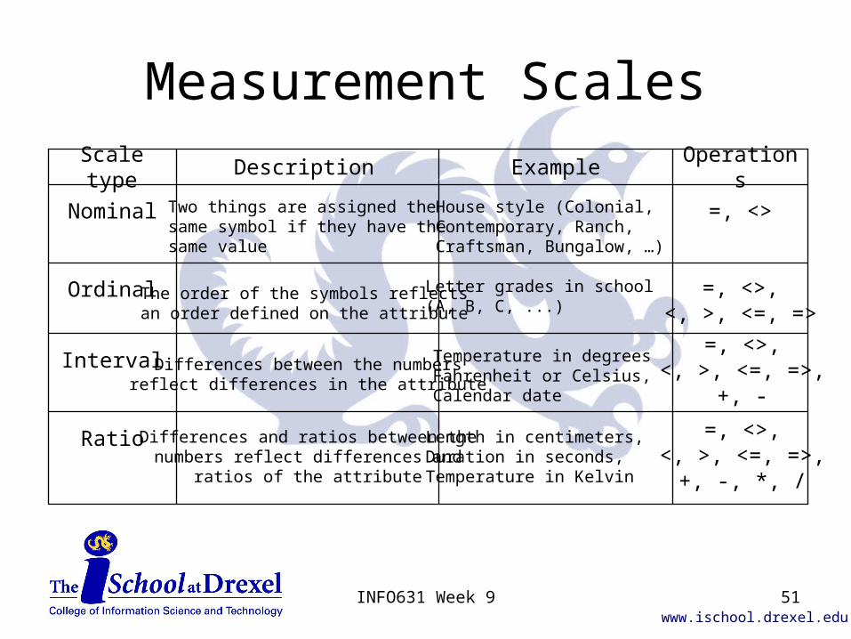
Measurement Scales
Scale type Description Example Operations
Nominal Two things are assigned the same symbol if they have thesame value
House style (Colonial,Contemporary, Ranch,Craftsman, Bungalow, …)
=, <>
Ordinal The order of the symbols reflectsan order defined on the attribute
Letter grades in school(A, B, C, ...)
=, <>,<, >, <=, =>
Interval Differences between the numbersreflect differences in the attribute
Temperature in degreesFahrenheit or Celsius,Calendar date
=, <>,<, >, <=, =>,
+, -
Ratio Differences and ratios between thenumbers reflect differences and
ratios of the attribute
Length in centimeters,Duration in seconds,Temperature in Kelvin
=, <>,<, >, <=, =>,
+, -, *, /
51INFO631 Week 9
www.ischool.drexel.edu
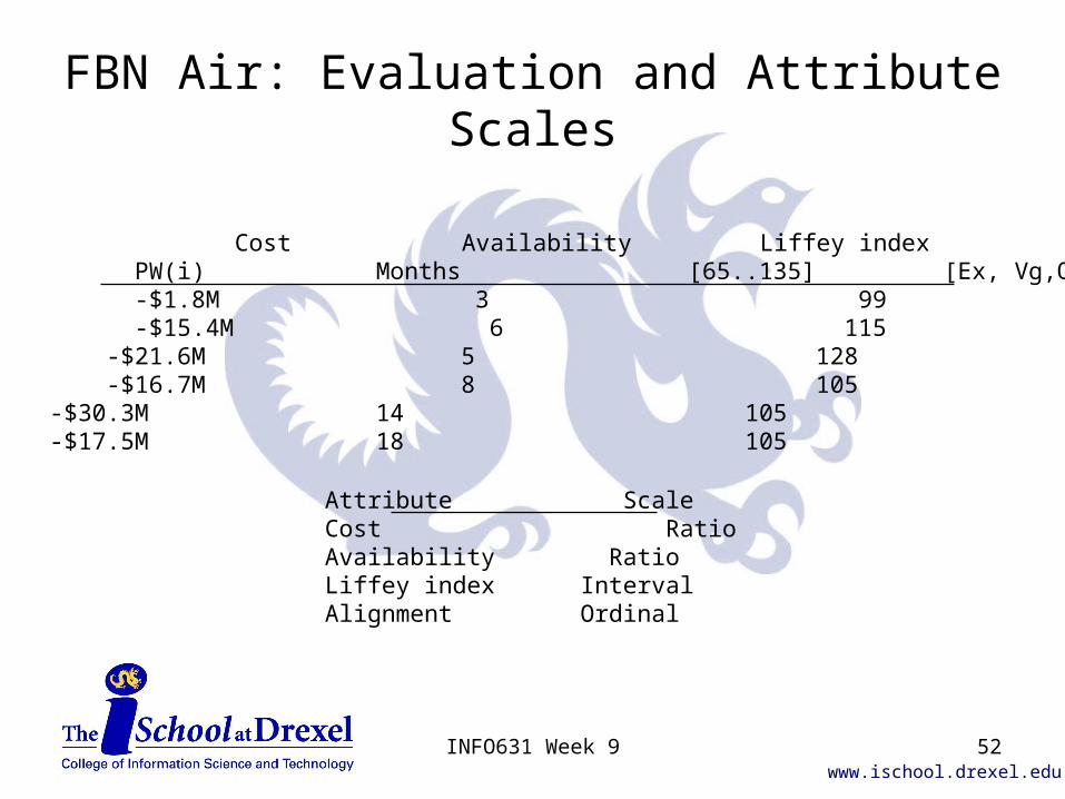
FBN Air: Evaluation and Attribute Scales
Cost Availability Liffey index AlignmentAlternative PW(i) Months [65..135] [Ex, Vg,Ok,Pr, Vpr]Existing -$1.8M 3 99 ExcellentJupiter -$15.4M 6 115 PoorSword -$21.6M 5 128 OkGuppy -$16.7M 8 105 Very poorNew in-house -$30.3M 14 105 ExcellentNew off-shore -$17.5M 18 105 Very good
Attribute ScaleCost RatioAvailability RatioLiffey index IntervalAlignment Ordinal
52INFO631 Week 9
www.ischool.drexel.edu
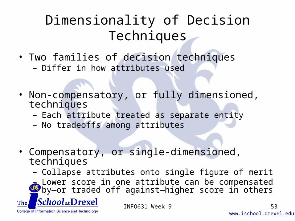
Dimensionality of Decision Techniques
• Two families of decision techniques– Differ in how attributes used
• Non-compensatory, or fully dimensioned, techniques– Each attribute treated as separate entity– No tradeoffs among attributes
• Compensatory, or single-dimensioned, techniques– Collapse attributes onto single figure of merit– Lower score in one attribute can be compensated by—or traded
off against—higher score in others
53INFO631 Week 9
www.ischool.drexel.edu
Non-compensatory Decision Techniques
• Three will be described– Dominance– Satisficing– Lexicography
54INFO631 Week 9
www.ischool.drexel.edu
Dominance• Compare each pair of alternatives on attribute-by-attribute basis
– Look for one alternative to be at least as good in every attribute and better in one or more
• When found, no problem deciding– One alternative is clearly superior to the other, inferior can be discarded
• May not lead to selecting one single alternative– Good for filtering alternatives and reducing work using other techniques
• In FBN Air, Jupiter dominates Guppy
55INFO631 Week 9
www.ischool.drexel.edu
Satisficing
• Sometimes called “method of feasible ranges”– Establish acceptable ranges of attribute
values– Alternatives with any attributes outside
acceptable range are discarded
• May not lead to selecting one single alternative– Good for filtering alternatives and reducing
work using other techniques56INFO631 Week 9
www.ischool.drexel.edu
Satisficing
• Can lead to selecting one alternative when used with an iterative propose-then-evaluate process
• Iterative version is appropriate when satisfactory performance, rather than optimal performance, is good enough– If optimal performance needed, always identify several
alternatives that meet satisficing criteria then do further decision analysis with one of other techniques
Repeat Propose a new solution Evaluate that solution against the decision attributesUntil the solution is within the acceptable range for all decision attributes
Note: Stops when 1st acceptable solution is proposed
57INFO631 Week 9
www.ischool.drexel.edu
Lexicography• Two previous techniques assume attributes have equal importance
– If one attribute is far more important than others, final choice could be made on that one attribute alone
• If alternatives have identical values for most-important attribute, use next-most-important attribute to break tie– If still tied, compare next most important attribute, …– Continue until a single alternative chosen or all alternatives evaluated
• FBN Air– Alignment might be #1, eliminates all but Existing and In-house– Cost might be #2, eliminates in-house
58INFO631 Week 9
www.ischool.drexel.edu
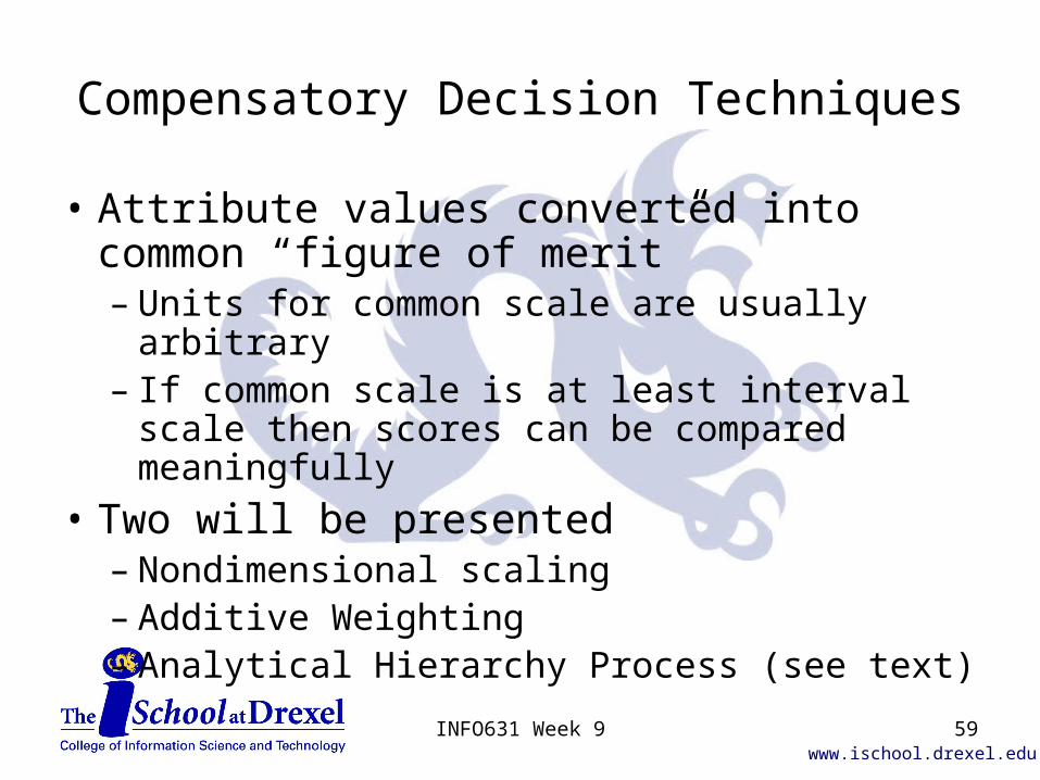
Compensatory Decision Techniques
• Attribute values converted into common “figure of merit”– Units for common scale are usually arbitrary– If common scale is at least interval scale then
scores can be compared meaningfully
• Two will be presented– Nondimensional scaling– Additive Weighting– Analytical Hierarchy Process (see text)
59INFO631 Week 9
www.ischool.drexel.edu
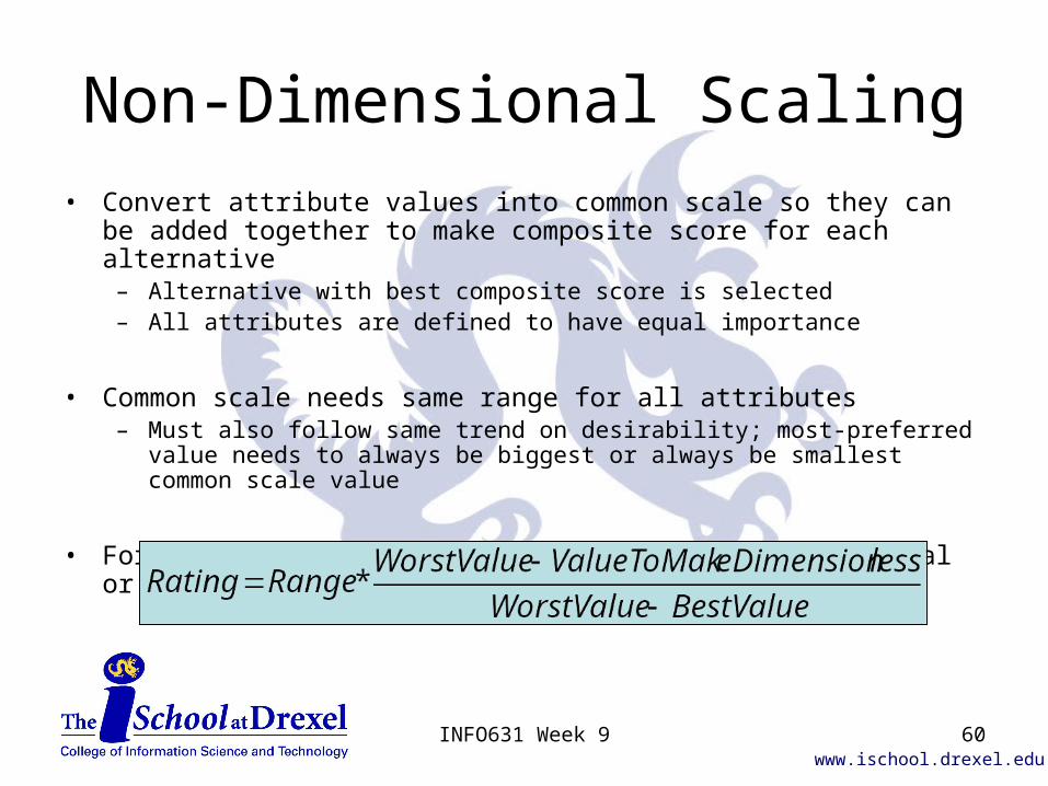
Non-Dimensional Scaling• Convert attribute values into common scale so they can be added together
to make composite score for each alternative– Alternative with best composite score is selected– All attributes are defined to have equal importance
• Common scale needs same range for all attributes– Must also follow same trend on desirability; most-preferred value needs to
always be biggest or always be smallest common scale value
• Formula for converting attributes, as long as interval or ratio-scaled, into the common scale
60INFO631 Week 9
www.ischool.drexel.edu
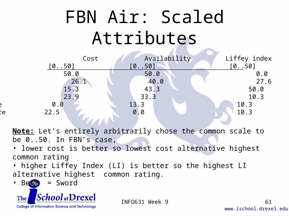
FBN Air: Scaled Attributes
Cost Availability Liffey indexAlternative [0..50] [0..50] [0..50] TotalExisting 50.0 50.0 0.0 100.0Jupiter 26.1 40.0 27.6 93.7Sword 15.3 43.3 50.0 108.6Guppy 23.9 33.3 10.3 67.5New in-house 0.0 13.3 10.3 23.6New off-shore 22.5 0.0 10.3 32.8
Note: Let’s entirely arbitrarily chose the common scale to be 0..50. In FBN’s case, • lower cost is better so lowest cost alternative highest common rating• higher Liffey Index (LI) is better so the highest LI alternative highest common rating.• Best = Sword
61INFO631 Week 9
www.ischool.drexel.edu
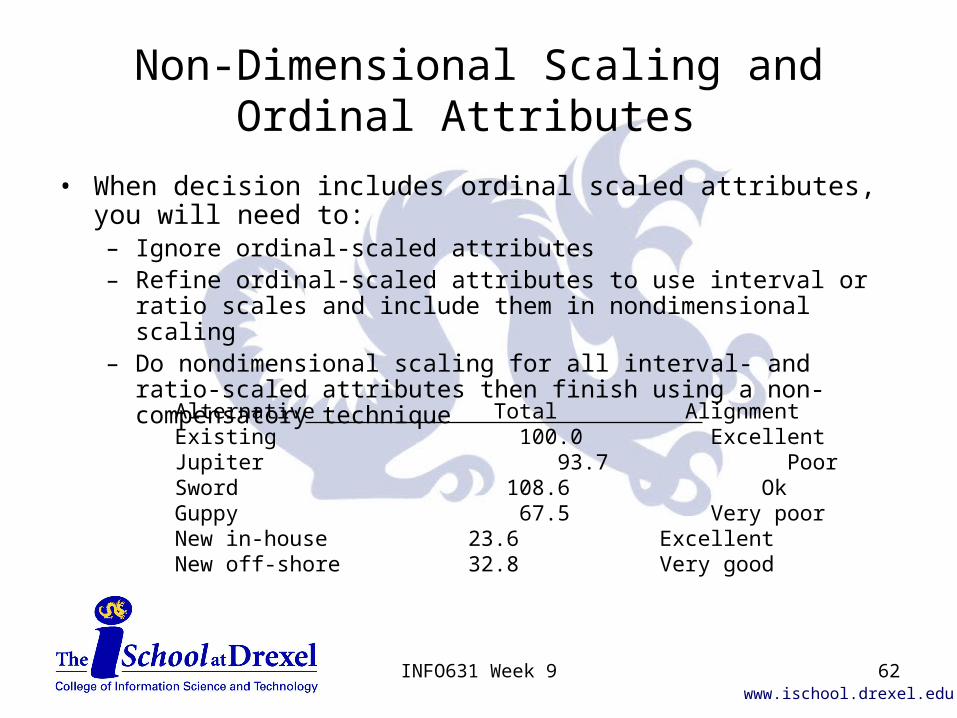
Non-Dimensional Scaling and Ordinal Attributes
• When decision includes ordinal scaled attributes, you will need to:– Ignore ordinal-scaled attributes– Refine ordinal-scaled attributes to use interval or ratio scales and
include them in nondimensional scaling– Do nondimensional scaling for all interval- and ratio-scaled attributes
then finish using a non-compensatory technique
Alternative Total AlignmentExisting 100.0 ExcellentJupiter 93.7 PoorSword 108.6 OkGuppy 67.5 Very poorNew in-house 23.6 ExcellentNew off-shore 32.8 Very good
62INFO631 Week 9
www.ischool.drexel.edu
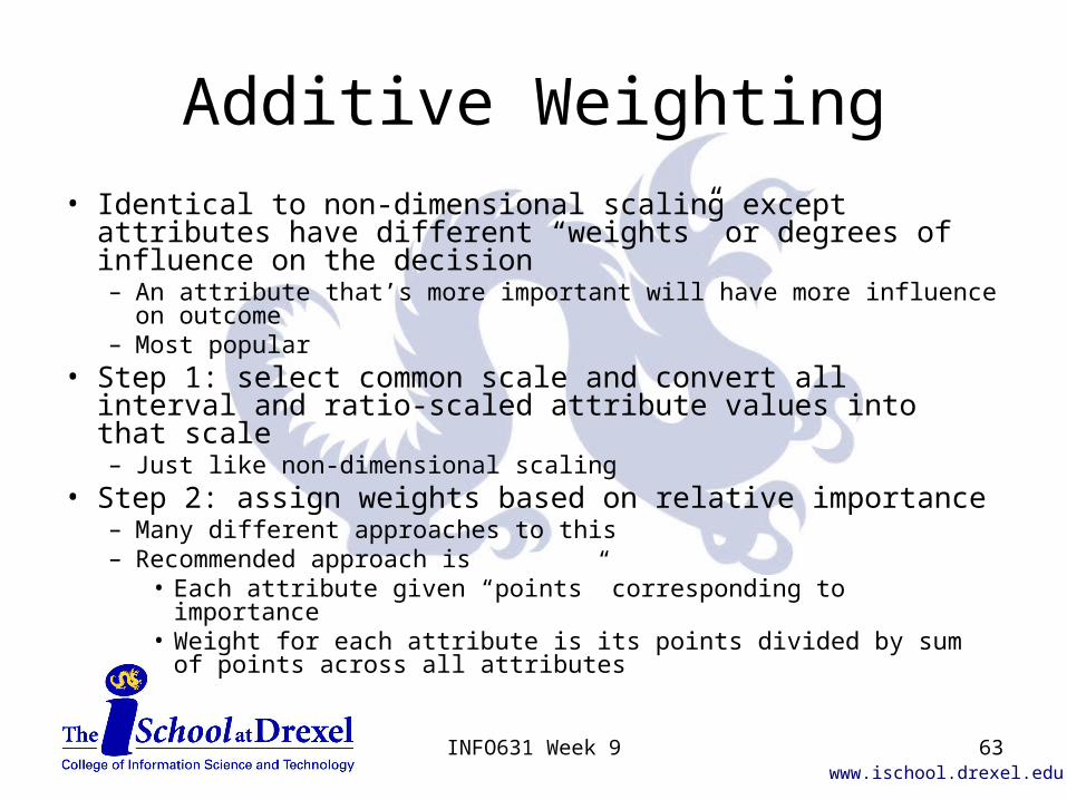
Additive Weighting
• Identical to non-dimensional scaling except attributes have different “weights” or degrees of influence on the decision– An attribute that’s more important will have more influence on
outcome– Most popular
• Step 1: select common scale and convert all interval and ratio-scaled attribute values into that scale– Just like non-dimensional scaling
• Step 2: assign weights based on relative importance– Many different approaches to this– Recommended approach is
• Each attribute given “points” corresponding to importance• Weight for each attribute is its points divided by sum of points
across all attributes63INFO631 Week 9
www.ischool.drexel.edu
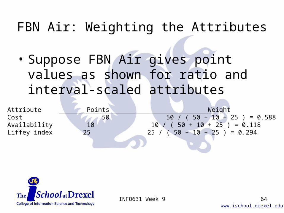
FBN Air: Weighting the Attributes
• Suppose FBN Air gives point values as shown for ratio and interval-scaled attributes
Attribute Points WeightCost 50 50 / ( 50 + 10 + 25 ) = 0.588Availability 10 10 / ( 50 + 10 + 25 ) = 0.118Liffey index 25 25 / ( 50 + 10 + 25 ) = 0.294
64INFO631 Week 9
www.ischool.drexel.edu
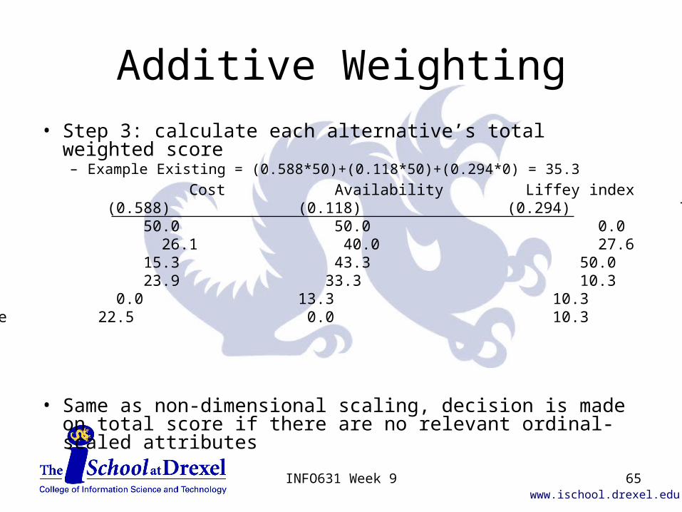
Additive Weighting
• Step 3: calculate each alternative’s total weighted score– Example Existing = (0.588*50)+(0.118*50)+(0.294*0) = 35.3
• Same as non-dimensional scaling, decision is made on total score if there are no relevant ordinal-scaled attributes
Cost Availability Liffey indexAlternative (0.588) (0.118) (0.294) TotalExisting 50.0 50.0 0.0 35.3Jupiter 26.1 40.0 27.6 28.2Sword 15.3 43.3 50.0 28.8Guppy 23.9 33.3 10.3 21.0New in-house 0.0 13.3 10.3 4.6New off-shore 22.5 0.0 10.3 16.3
65INFO631 Week 9
www.ischool.drexel.edu
Key Points• Aside from technical feasibility, money is almost always the most important
decision criterion but it’s not always the only one• Use values can usually be quantified in terms of money• Esteem values can't be quantified in terms of money
– Decisions involving more than one attribute are almost inevitable• Choose decision attributes to cover all relevant use values and esteem
values• Several different classes of measurement
– Nominal, Ordinal, Interval, and Ratio– Within each class, some comparisons will make sense and others won’t
• Non-compensatory techniques treat each attribute as a separate entity– Dominance, Satisficing, Lexicography
• Compensatory techniques allow better performance on one attribute to compensate for poorer performance in another
– Nondimensional Scaling, Additive Weighting
66INFO631 Week 9