Embed Size (px)
Citation preview

Writing Scilab Extensions
Michael Baudin
July 2012
Abstract
In this document, we present methods to use and create Scilab extensions.In the first part, we focus on the use of external modules. We describe
their general organization and how to install a module from ATOMS. Thenwe describe how to build a module from the sources. In the second part, wepresent the management of a toolbox, and the purpose of each directory. Weemphasize the use of simple methods to automatically create the help pagesand to manage the unit tests. Then we present the creation of interfaces,which allows to connect Scilab to a compiled C, C++ or Fortran library.We consider the example of a simple function in the C language and exploreseveral ways to make this function available to Scilab. We consider a simplemethod based on exchanging data by file. We then present a method basedon the call function. Finally, we present the classical, but more advanced,method to create a gateway and how to use the Scilab API. The two lastsections focus on designing issues, such as managing the optional input oroutput arguments or designing examples.
Contents
1 Introduction 5
2 Extending Scilab capabilities 52.1 Introduction . . . . . . . . . . . . . . . . . . . . . . . . . . . . . . . . 52.2 Types of external modules . . . . . . . . . . . . . . . . . . . . . . . . 62.3 Using ATOMS . . . . . . . . . . . . . . . . . . . . . . . . . . . . . . 62.4 The toolbox skeleton . . . . . . . . . . . . . . . . . . . . . . . . . . . 72.5 A sample module . . . . . . . . . . . . . . . . . . . . . . . . . . . . . 82.6 The internal structure of a module . . . . . . . . . . . . . . . . . . . 82.7 Building an external module from the sources . . . . . . . . . . . . . 92.8 Using a module . . . . . . . . . . . . . . . . . . . . . . . . . . . . . . 102.9 Loading the module automatically . . . . . . . . . . . . . . . . . . . . 102.10 Cleaning the module (*) . . . . . . . . . . . . . . . . . . . . . . . . . 112.11 Scilab’s Forge (*) . . . . . . . . . . . . . . . . . . . . . . . . . . . . . 11
1

3 Managing a module 123.1 The tbx module . . . . . . . . . . . . . . . . . . . . . . . . . . . . . . 123.2 The chain of builders . . . . . . . . . . . . . . . . . . . . . . . . . . . 143.3 The main builder . . . . . . . . . . . . . . . . . . . . . . . . . . . . . 143.4 The etc directory . . . . . . . . . . . . . . . . . . . . . . . . . . . . . 153.5 The macros directory . . . . . . . . . . . . . . . . . . . . . . . . . . . 183.6 Creating private functions (*) . . . . . . . . . . . . . . . . . . . . . . 193.7 The help directory . . . . . . . . . . . . . . . . . . . . . . . . . . . . 203.8 Help pages in local languages (*) . . . . . . . . . . . . . . . . . . . . 233.9 Advanced help pages (*) . . . . . . . . . . . . . . . . . . . . . . . . . 243.10 Creating help chapters (*) . . . . . . . . . . . . . . . . . . . . . . . . 263.11 The tests directory . . . . . . . . . . . . . . . . . . . . . . . . . . . 273.12 Executing the unit tests . . . . . . . . . . . . . . . . . . . . . . . . . 283.13 Advanced unit tests (*) . . . . . . . . . . . . . . . . . . . . . . . . . . 303.14 Issues with unit tests . . . . . . . . . . . . . . . . . . . . . . . . . . . 313.15 The assert module . . . . . . . . . . . . . . . . . . . . . . . . . . . . 323.16 Advanced assert use-cases (*) . . . . . . . . . . . . . . . . . . . . . 353.17 Generating the help from the macros . . . . . . . . . . . . . . . . . . 373.18 Using pseudomacros (*) . . . . . . . . . . . . . . . . . . . . . . . . . 393.19 A check-list for the module . . . . . . . . . . . . . . . . . . . . . . . . 39
4 Interfaces (*) 394.1 Overview . . . . . . . . . . . . . . . . . . . . . . . . . . . . . . . . . 404.2 A sample function . . . . . . . . . . . . . . . . . . . . . . . . . . . . . 414.3 By files . . . . . . . . . . . . . . . . . . . . . . . . . . . . . . . . . . . 414.4 With the call function . . . . . . . . . . . . . . . . . . . . . . . . . . 47
4.4.1 The C source code . . . . . . . . . . . . . . . . . . . . . . . . 474.4.2 Debugging with ilib_for_link . . . . . . . . . . . . . . . . . 484.4.3 Using call . . . . . . . . . . . . . . . . . . . . . . . . . . . . 50
4.5 With a gateway . . . . . . . . . . . . . . . . . . . . . . . . . . . . . . 524.5.1 Scilab data structures . . . . . . . . . . . . . . . . . . . . . . 524.5.2 The Scilab API . . . . . . . . . . . . . . . . . . . . . . . . . . 534.5.3 Analysis of a gateway . . . . . . . . . . . . . . . . . . . . . . . 544.5.4 Debugging a gateway . . . . . . . . . . . . . . . . . . . . . . . 59
4.6 A module with gateways . . . . . . . . . . . . . . . . . . . . . . . . . 604.6.1 The src directory . . . . . . . . . . . . . . . . . . . . . . . . . 604.6.2 The src/* subdirectories . . . . . . . . . . . . . . . . . . . . . 614.6.3 The sci_gateway directory . . . . . . . . . . . . . . . . . . . 654.6.4 The sci_gateway/* subdirectories . . . . . . . . . . . . . . . 664.6.5 Solving compilation issues . . . . . . . . . . . . . . . . . . . . 68
5 Designing the module 715.1 Introduction . . . . . . . . . . . . . . . . . . . . . . . . . . . . . . . . 715.2 Avoid function name conflicts . . . . . . . . . . . . . . . . . . . . . . 715.3 Optional input arguments . . . . . . . . . . . . . . . . . . . . . . . . 725.4 Provide as many input arguments as reasonable . . . . . . . . . . . . 735.5 A correct order for optional input arguments . . . . . . . . . . . . . . 73
2

5.6 A correct order for optional output arguments . . . . . . . . . . . . . 745.7 Argument checking . . . . . . . . . . . . . . . . . . . . . . . . . . . . 755.8 Localization of messages (*) . . . . . . . . . . . . . . . . . . . . . . . 765.9 Output messages within functions . . . . . . . . . . . . . . . . . . . . 765.10 Orthogonality between modules (*) . . . . . . . . . . . . . . . . . . . 775.11 Do not stay alone : communicate! . . . . . . . . . . . . . . . . . . . . 785.12 A check-list for the API . . . . . . . . . . . . . . . . . . . . . . . . . 79
6 Designing examples 796.1 Any function has one (or more) example . . . . . . . . . . . . . . . . 796.2 Examples are self-contained . . . . . . . . . . . . . . . . . . . . . . . 80
7 section-sciext-exampleselfcontained 807.1 Only valid statements . . . . . . . . . . . . . . . . . . . . . . . . . . . 807.2 Provide scripts, not sessions . . . . . . . . . . . . . . . . . . . . . . . 807.3 Let the user see the results . . . . . . . . . . . . . . . . . . . . . . . . 817.4 A good example . . . . . . . . . . . . . . . . . . . . . . . . . . . . . . 817.5 A check-list for the examples . . . . . . . . . . . . . . . . . . . . . . . 82
8 Notes and references 82
Bibliography 83
Index 83
3

Copyright c© 2012 - Michael BaudinThis file must be used under the terms of the Creative Commons Attribution-
ShareAlike 3.0 Unported License:
http://creativecommons.org/licenses/by-sa/3.0
4

1 Introduction
This document is an open-source project. The LATEXsources are available on theScilab Forge:
http://forge.scilab.org/index.php/p/docsciextensions/
The LATEXsources are provided under the terms of the Creative Commons Attri-bution-ShareAlike 3.0 Unported License:
http://creativecommons.org/licenses/by-sa/3.0
2 Extending Scilab capabilities
In this section, we present Scilab external modules, a system which allows to extendconsiderably the capabilities of Scilab. In the first part, we present the basic methodto install Scilab modules. In the second part, we present a sample use of the ATOMScomponent, a packaging system for Scilab.
In this document, the sections marked with an asterisk (*) can be considered asoptional and can be skipped in a first reading.
2.1 Introduction
One of the most interesting features of Scilab is that we can use and create exten-sions, which behave as built-in functions. The simplicity of creating these extensionshas make so that there are hundreds of public extensions publicly available. Thiswealth of extensions is already a great source of information to create our own mod-ules. In this document, we present the most common methods to create new basicmodules and some advanced methods to make the creation easier when a lot offunctions are involved, or when a compiled source code is involved.
Although the word toolbox has been used in the past, the word module is nowemployed in the context of Scilab, with two different meanings.
• An internal module is a component which is provided by Scilab itself.
• An external module is a component which is not provided by Scilab, but canbe loaded by Scilab to extend its features.
Fortunately, although they are technically a bit different, internal and external mod-ules have a lot in common so that understanding the latter is an excellent introduc-tion to the former.
The topics that we present in this document are simple, but relatively advanced,in the sense that many users never have to extend Scilab features because they arehappy with the features already provided. Nevertheless, when it comes to extendingScilab features, we have to already master the more regular features that many usersalready know.
We suggest to read the documents [2] and [3] for topics which might be unclearwhen reading the current document.
5

More precisely, we suggest to fully master the sections 2.8 ”ATOMS, the pack-aging system of Scilab” and the section 6 ”Functions” in [2]. This should be a goodbasis for the section 3 of the current document.
The section 4 ”Management of functions” in [3] should be a consistent help forthose searching how to design functions. This should be a good basis for the moreadvanced topics in the section 5 of the current document.
2.2 Types of external modules
A Scilab module is a set of macros, help files and unit tests, which enhance Scilabwith new features. Notice that some modules also contain compiled source code (e.g.in the C language), but most modules are only based on macros. External modulesare meant to be developed and maintained by Scilab users, but some modules aredeveloped or maintained by the Scilab core development team.
Modules can be distinguished on the base of the origin of the features:
• modules based only on macros (i.e. functions),
• modules based only on compiled source code (i.e. Fortran, C or C++),
• modules based both on macros and compiled source code.
This difference is critical, since compiling a library requires a compiler (e.g. gcc onGnu/Linux or Visual Studio on MS Windows). This is generally a non trivial task.In practice, when we get an external module based on compiled source code, it maybe difficult to generate a binary version of this module. The ATOMS system hasbeen designed for that purpose, in order to make the installation of external modulesan easy process. The ATOMS system is reviewed in the next section.
2.3 Using ATOMS
ATOMS is the Scilab tool which allows to search, download, install and load mod-ules. The ATOMS system is available in Scilab since version 5.2. The homepage forthe ATOMS system is the following:
http://atoms.scilab.org
The ATOMS system allows to install and use external modules without the bur-den of compiling the module, a task which is generally difficult and time consuming.Moreover, any external module which is packaged in the ATOMS system is guar-anteed to be loadable in Scilab. We cannot be sure that the functions are bugfree,but, at least, we are sure that the module can be loaded in our current version ofScilab.
In this section, we consider the NISP module, which provide functions to performsensitivity analysis in uncertainty quantification. This is a good example, since theNISP module is based on a C++ library: building this module requires a compiler.Fortunately, the NISP module has been packaged in ATOMS:
http://atoms.scilab.org/toolboxes/NISP
6

The NISP module is available for the following platforms:
• Windows 32 bit, 64 bit,
• Linux 32 bit, 64 bit,
• Mac OS X.
The ATOMS component allows to install and use the NISP module, without havinga compiler installed in the system.
In the following Scilab session, we use the atomsInstall() function to downloadand install the binary version of the module corresponding to the current operatingsystem.
-->atomsInstall("NISP")
ans =
!NISP 2.1 allusers D:\ Programs\SC3623 ~1\ contrib\NISP \2.1 I !
Then we restart Scilab. At the startup, we see the following messages in the console:
Start NISP Toolbox
Load gateways
Load help
Load demos
showing that the module is available. The NISP module has been automaticallyloaded at the start of the Scilab session.
In order to remove the NISP module, we just use the atomsRemove function.More details on ATOMS are available at [11].
2.4 The toolbox skeleton
Developing a new module is designed to be as easy as possible. For this purpose, amodule skeleton is provided within Scilab, in the SCI/contrib/toolbox_skeleton
directory, or in the Git repository:
http://gitweb.scilab.org/?p=scilab.git;a=tree;f=scilab/contrib/
toolbox_skeleton
This module is made of both macros and compiled source code, and presentsseveral methods required to manage a module. One of the interests of the toolboxskeleton is that it allows to separate what are the files which must be edited by thedevelopper, and what are the files which are automatically generated by Scilab.
Notice that a toolbox skeleton for Xcos blocks is also available at:
http://atoms.scilab.org/toolboxes/xcos_toolbox_skeleton
Of course, the toolbox skeleton could be used in this document to present themethods to write Scilab extensions. The difficulty with this skeleton is that it usescompiled sources codes, which is a more advanced topic and is not used by manyusers. The section 4 presents the interfaces in Scilab. Hence, we suggest to read thetoolbox skeleton as a pratical exercise of this document, but after having practicingthe more simple example that we now consider.
The next section presents the number module, which will be used in this docu-ment.
7

2.5 A sample module
An external module must respect standards about its internal organization. Inorder to describe this organization, we will consider the practical case of the numbermodule.
The latest version of this module can be dowloaded at:
http://atoms.scilab.org/toolboxes/number
The module is developed on the Forge at:
http://forge.scilab.org/index.php/p/number
It is easy to download a zip file containing the sources of the number module at:
http://forge.scilab.org/index.php/p/number/downloads
The number module provides several algorithms which are related to numbertheory, for example the greatest common divisor or prime factorization. In thefollowing sections, we assume that we have downloaded a source version of thenumber module, so that we have the associated number.zip file.
The reason why we consider the number module is because it is an example ofa module which only uses Scilab macros. Hence, building this module is relativelysimple.
We now want to make a binary version of this module. Before, analysing themethod to do this, we are going to review the internal structure of a module.
2.6 The internal structure of a module
In this section, we analyze the internal organization of an external module.The following list is an overview of the content of the directories.
• number/demos: demonstration scripts (.sce files),
• number/etc: startup and shutdown scripts for the module,
• number/help: help pages (.xml files),
• number/macros: macros (.sci files),
• number/tests: unit and non regression tests.
These are all the directories required in the number module. But, if the module, saymytoolbox for example, contains compiled source codes, then we should have thefollowing extra directories.
• mytoolbox/sci_gateway: the sources of the gateway (.c or .cpp files),
• mytoolbox/src: the sources of the library (.f, .c or .cpp files).
At the root of the module, the following files are usually located.
• number/builder.sce: the script which ”builds” the module,
8
• number/changelog.txt: the changes from version to version,
• number/licence.txt: the license of the module,
• number/readme.txt: the purpose of the module.
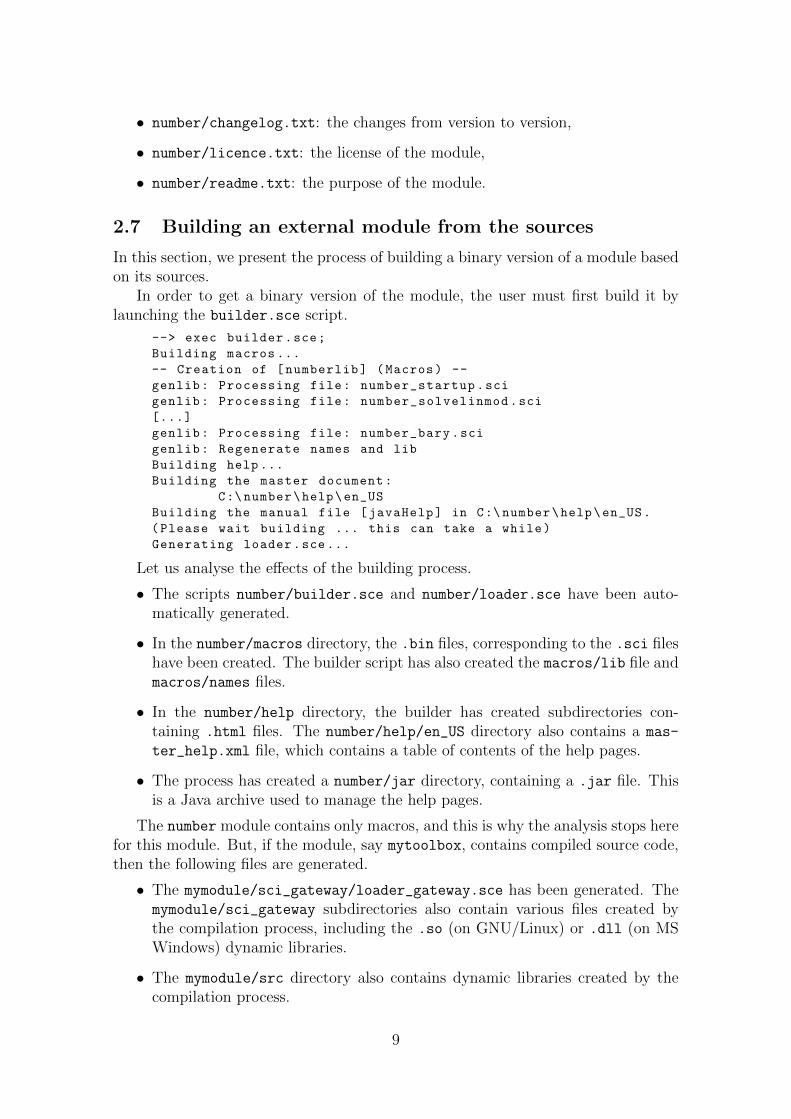
2.7 Building an external module from the sources
In this section, we present the process of building a binary version of a module basedon its sources.
In order to get a binary version of the module, the user must first build it bylaunching the builder.sce script.
--> exec builder.sce;
Building macros ...
-- Creation of [numberlib] (Macros) --
genlib: Processing file: number_startup.sci
genlib: Processing file: number_solvelinmod.sci
[...]
genlib: Processing file: number_bary.sci
genlib: Regenerate names and lib
Building help ...
Building the master document:
C:\ number\help\en_US
Building the manual file [javaHelp] in C:\ number\help\en_US.
(Please wait building ... this can take a while)
Generating loader.sce...
Let us analyse the effects of the building process.
• The scripts number/builder.sce and number/loader.sce have been auto-matically generated.
• In the number/macros directory, the .bin files, corresponding to the .sci fileshave been created. The builder script has also created the macros/lib file andmacros/names files.
• In the number/help directory, the builder has created subdirectories con-taining .html files. The number/help/en_US directory also contains a mas-
ter_help.xml file, which contains a table of contents of the help pages.
• The process has created a number/jar directory, containing a .jar file. Thisis a Java archive used to manage the help pages.
The number module contains only macros, and this is why the analysis stops herefor this module. But, if the module, say mytoolbox, contains compiled source code,then the following files are generated.
• The mymodule/sci_gateway/loader_gateway.sce has been generated. Themymodule/sci_gateway subdirectories also contain various files created bythe compilation process, including the .so (on GNU/Linux) or .dll (on MSWindows) dynamic libraries.
• The mymodule/src directory also contains dynamic libraries created by thecompilation process.
9

2.8 Using a module
In this section, we present how to use a module which has been previously trans-formed into binary form.
After we have built the module, the main directory now contains a number/
loader.sce. In order to load the library, we now execute the loader.sce script.
-->exec C:\ number\loader.sce;
Start Number
Load macros
Load help
Load demos
Type "help number_overview" for quick start.
Type "demo_gui ()" and search for Number
for Demonstrations.
We can now use the module, as if the functions were built in Scilab.
-->number_gcd (4,6)
ans =
2.
The statement
-->help number_gcd
opens the help browser and shows the help page of the number_gcd function.We can also see and execute the demonstrations of this module. In order to do
this, a first method is to open the ”? > Scilab Demonstrations” menu at the rightof the main menu of the console. The second method is to execute the demo_gui
function, as in the following session.
-->demo_gui ()
Both methods open the demonstration browser, where we can find the ”Number”section. When we click on the entries of the ”Number” section, some scripts areexecuted. These scripts either print messages in the console or produce graphics.In some cases, the script containing the demonstration is opened within the editor,which let us see how the functions of the number module were used to produce theseoutputs.
2.9 Loading the module automatically
In this section, we present a method to automatically load a module, thanks toScilab’s startup file.
We can easily configure Scilab so that the module is automatically loaded atstartup. It suffices to add a line in the .scilab file associated with the currentScilab system. In order to locate the directory associated with the automatic startupsystem, we can display the value of the SCIHOME variable.
-->SCIHOME
SCIHOME =
C:\ DOCUME ~1\ Root\APPLIC ~1\ Scilab\scilab -5.2.0 -beta -1
Then, we edit the file
C:\ DOCUME ~1\ Root\APPLIC ~1\ Scilab\scilab -5.2.0 -beta -1\. scilab
10
or we create it if it does not exist. We may also use the editor to directly open thefile, with the following statement:
editor(fullfile(SCIHOME ,".scilab"))
In this file, we write the line
exec("C:\ number\loader.sce");
which executes the loader script associated with the module. Now, if we exit fromScilab and start it again, the module is automatically loaded.
2.10 Cleaning the module (*)
In this section, we present the cleaner script, which can be used to delete the binaryfiles which have been generated by the building process.
The builder script has created a number/cleaner.sce script, which can deleteall the files which have been created by the builder script. In order to use this script,we just have to execute it:
-->exec("C:\ number\cleaner.sce");
In fact, this script is a tool dedicated to the developper of the module. It can beused, for example, after some preliminary builds, to check that the building processexecutes correctly when it starts from zero.
2.11 Scilab’s Forge (*)
Scilab forge is a tool for external modules developers, which can help the develop-ment process.
The main adress of the Scilab Forge is:
http://forge.scilab.org/index.php/projects/
The Scilab Forge is the place where we can share the source code of Scilabprojects. It provides several components to make the development easier. Moreprecisely, it provides
• a source code revision system (SVN or GIT),
• a Download system (to upload and download module releases, documents inpdf form or binaries),
• documentation pages (as a wiki),
• a bug tracker,
and several other features as well. The Forge lets the developers work on a commonsource code as a team, even if the developers are not in the same location.
When we use the Forge as a regular Scilab user, we can
• download the releases,
• report bugs,
11

• browse the source code with a web browser.
When we use the Forge as a developer, it is mandatory to be familiar with versionmanagement systems such as SVN or GIT. For example, the developer can
• update the source code with SVN or GIT,
• manage the bug reports,
• upload the releases.
The Scilab Forge is also a good place to find sources of modules. This can behelpful, for example when we search for a new technical feature.
More details on Scilab’s Forge are presented at:
http://wiki.scilab.org/Scilab%20forge
3 Managing a module
In this section, we present how to manage a module. We analyse the tbx module,which is used in all standard modules to make the building process easier. In theremaining of the section, we present the various scripts and directories of a moduleand analyse their contents.
3.1 The tbx module
The tbx module is a built-in module which let us develop new modules. It providesa set of functions to compile a module and to produce the binary version of themodule.
The figure 1 presents the main functions of the tbx module.In order to understand the tbx module, we must distinguish the various types
of scripts within a module.
• A builder is a script which executes statements which convert a source code(either with .sci, .c, .cpp or .f file extension) into a binary file, and au-tomatically generates the scripts required to load or clean the module. Thebuilder is written by the developper of the module.
• A loader is a script which executes statements to load the binaries in Scilab.These binaries can be the .bin associated with macros, the Java archive (jar)associated with the help or the binaries associated with the source codes orgateways (.so or .dll). The loader is automatically generated by the tbx
module.
• A cleaner is a script which executes statements to delete the files automaticallycreated by the builder. The loader is automatically generated by the tbx
module.
12

Main functionstbx_build_cleaner Generate a cleaner.sce scripttbx_build_loader Generate a loader.sce scriptMacrostbx_build_macros Compile macrostbx_builder_macros Run buildmacros.sce script if it existsHelptbx_build_help Generate help filestbx_build_help_loader Generate a addchapter.sce scripttbx_builder_help Run builder_help.sce script if it existstbx_builder_help_lang Run build_help.sce script if it existsGateways (*)tbx_build_gateway Build a gatewaytbx_build_gateway_clean Generate a cleaner_gateway.sce scripttbx_build_gateway_loader Generate a loader_gateway.sce scripttbx_builder_gateway Run builder_gateway.sce script if it existstbx_builder_gateway_lang Run builder_gateway_(language).sce
script if it existsSources (*)tbx_build_src Build sourcestbx_builder_src Run builder_src.sce script if it existstbx_builder_src_lang Run builder_(language).sce script if it existsXcos (*)tbx_build_blocks Compile blocks
Figure 1: The tbx module. Sections marked with (*) are optional.
13

Thanks to the tbx module, there are very few scripts which must be edited by thedeveloper: most other scripts are automatically generated by the tbx functions.
For each type of directory (i.e. macros, help, sources, gateways and Xcos blocks),the tbx module provides two types of functions:
• the tbx_builder_* functions just executes sub-builders in the correspondingsub-directories,
• the tbx_build_* functions actually converts the sources into binary files orautomatically generates other scripts.
The tbx_builder_* functions will become clearer in the next section, when wediscuss the chain of builders.
3.2 The chain of builders
The builders of a module are a set of scripts, with the .sce file extension. Buildingthe module just consists in executing the main builder.sce, which performs someprocessing and executes, in turn, other sub-builders. For example, we may considerthe following chain of builders.
• number/builder.sce: main builder,
• number/macros/buildmacros.sce: convers the .sci macros into binary files,
• number/help/builder_help.sce: builds the help pages.
When we execute the number/builder.sce script, the tbx functions that we call willexecute first the number/macros/ buildmacros.sce script, then the number/help/
builder_help.sce script. In fact, this is not done directly in the script, but ratherimplicitely by the tbx functions which know what scripts to execute, provided thatwe follow the standards.
3.3 The main builder
The main builder has the role of executing other sub-builders in appropriate sub-directories, and performing other treatments as well. For example, the main builderof the number module is the following.
function buildNumberMain ()
try
getversion("scilab");
catch
error(gettext("Scilab 5.0 or more is required."));
end;
if ~with_module("development_tools") then
error(msprintf (..
gettext("%s module not installed."),..
"development_tools"));
end
TOOLBOX_NAME = "number";
TOOLBOX_TITLE = "Number";
14

toolbox_dir = get_absolute_file_path("builder.sce");
tbx_builder_macros(toolbox_dir );
tbx_builder_help(toolbox_dir );
tbx_build_loader(TOOLBOX_NAME , toolbox_dir );
tbx_build_cleaner(TOOLBOX_NAME , toolbox_dir );
endfunction
buildNumberMain ();
clear buildNumberMain
Let us analyse the previous script in more details.The call to the tbx_builder_macros function has the effect of executing the num-
ber/macros/ buildmacros.sce script. Similarly, the call to the tbx_builder_helpfunction has the effect of executing the number/help/builder_help.sce script.The tbx_build_loader function generates the number/loader.sce script, whichcan be used later to load the module. Finally, the tbx_build_cleaner functiongenerates the number/cleaner.sce script, which can be used later to clean themodule.
The clear buildNumberMain statement prevents the function buildNumber-
Main from being visible from the user. Indeed, this function would have no sensefor a regular user, for whom the building process must, in general, stay invisible.The reason why the body of this builder in inside a function is because it limits thenumber of clear statements to be performed.
The main output of the main builder is the loader.sce script, which allows toload the module.
3.4 The etc directory
The etc directory contains two scripts which are executed when the module is loaded(e.g. when Scilab starts) and when Scilab quits.
• number/etc/number.start: this script is executed when the module starts,
• number/etc/number.quit: this script is executed when Scilab quits.
When we execute the number/loader.sce script, we see the following messagesin the console.
-->exec L:\ mypath\number\loader.sce;
Start Number
Load macros
Load help
Load demos
Type "help number_overview" for quick start.
Type "demo_gui ()" and search for Number
for Demonstrations.
The previous messages are printed by the number/etc/number.start script thatwe are going to analyse.
The content of the number/etc/number.start script is presented below.
function numberlib = loadnumberlib ()
TOOLBOX_NAME = "number"
TOOLBOX_TITLE = "Number"
15

mprintf("Start %s\n",TOOLBOX_TITLE );
etc_tlbx = get_absolute_file_path(TOOLBOX_NAME +..
".start");
etc_tlbx = getshortpathname(etc_tlbx );
root_tlbx = strncpy( etc_tlbx , ..
length(etc_tlbx)-length("\etc\") );
// Load functions library
if ( %t ) then
mprintf("\tLoad macros\n");
pathmacros = pathconvert( root_tlbx ) + ..
"macros" + filesep ();
numberlib = lib(pathmacros );
end
// Load gateways
if ( %f ) then
mprintf("\tLoad gateways\n");
ilib_verbose (0);
exec( pathconvert(root_tlbx +..
"/sci_gateway/loader_gateway.sce",%f));
end
// Load and add help chapter
if or(getscilabmode () == ["NW";"STD"]) then
mprintf("\tLoad help\n");
path_addchapter = pathconvert(root_tlbx+"/jar");
if ( isdir(path_addchapter) <> [] ) then
add_help_chapter(TOOLBOX_TITLE , ..
path_addchapter , %F);
end
end
// Add demos
if or(getscilabmode () == ["NW";"STD"]) then
mprintf("\tLoad demos\n");
demoscript = TOOLBOX_NAME + ".dem.gateway.sce"
pathdemos = pathconvert(fullfile(root_tlbx ,..
"demos",demoscript),%f,%t);
add_demo(TOOLBOX_TITLE ,pathdemos );
end
// A Welcome message.
mprintf("\tType ""help number_overview"" for "+..
"quick start.\n");
mprintf("\tType ""demo_gui ()"" and search for "+..
TOOLBOX_TITLE+" for Demonstrations .\n");
endfunction
if ( isdef("numberlib") ) then
warning("\tLibrary is already loaded (""ulink (); "+..
"clear numberlib;"" to unload .)");
return;
end
16

numberlib = loadnumberlib ();
clear loadnumberlib;
The previous script has been written so that it is easy to customize parts of thescript in order to adapt it to new modules. For example, it is easy to change thecontent of the variables TOOLBOX_NAME and TOOLBOX_TITLE in order to adapt to anew module name.
Let us analyse the script in more detail.The TOOLBOX_NAME variable just contains the lower case name of the module.
It is used to compute automatically file names, such as the number/demos/ num-
ber.dem.gateway.sce script, for example.On the other hand, the TOOLBOX_TITLE variable contains the capitalized module
name, which is used to print messages to the user. For example, the message thatwe see at startup:
Start Number
is generated from the content of the TOOLBOX_TITLE variable. Similarily, the TOOL-
BOX_TITLE variable is used to create the help and demonstrations sections.The call to the get_absolute_file_path function could be expressed as the
statement:
etc_tlbx=get_absolute_file_path("number.start");
This sets the etc_tlbx variable to the string containing the absolute path of thenumber.start script. This allows to compute the variable root_tlbx, which is setto the absolute main directory of the module. The remaining of the script uses thisvariable to compute other relative directories in the module, such as the path to thejar containing the help pages, for example.
The following statement:
if ( %f ) then
is used to disable the block of code corresponding to the loading of the gateways.Indeed, in the particular case of the number module, there is no compiled sourcecode and not gateway. But, if the module was to contain a gateway, we would justreplace the %f by a %t, and the code would then load the gateways automatically.
The variable numberlib plays a particularly important role, because it containsinformations that are used by Scilab to find the functions in the module. Thisvariable is created by the statement:
numberlib = lib(pathmacros );
The numberlib must be a global variable, and this is why it is the output argumentof the loadnumberlib function. We can see the content of this variable, as in thefollowing session.
-->numberlib
numberlib =
Functions files location : L:\ mypath\number\macros \.
number_addgroupmod number_barygui [...]
The variable contains both the path where the functions are located and the list ofall the functions in the library.
17

Hence, if the numberlib variable already exists when the module starts, thismeans that the module has been loaded twice. In this case, an error message isgenerated and the module is not loaded again, as in the following session.
-->exec L:\ mypath\number\loader.sce;
Start Number
Load macros
Load help
Load demos
Type "help number_overview" for quick start.
Type "demo_gui ()" and search for Number for
Demonstrations.
-->exec L:\ mypath\number\loader.sce;
WARNING: Library is already loaded ("ulink ();
clear numberlib;" to unload .)
In the case of the number module, the number/etc/number.quit file is empty,although the file must exist. This file may be used in some particular cases whensome cleanup must be executed when Scilab quits. For example, the quit script maybe used in one of the following situations.
• One or several files must be closed, or deleted.
• Some memory must be deallocated.
3.5 The macros directory
In this section, we present the macros directory, which contains the functions pro-vided in .sci files.
In the macros directory, we find regular .sci files containing function definitions.For example, the content of the number_coprime.sci file could just be the following.This function returns true if the greatest common divisor of the input arguments m
and n is equal to 1.
function arecoprime = number_coprime ( m , n )
d = number_gcd ( m , n )
arecoprime = ( d == 1 )
endfunction
The number of .sci files in the macros directory is not limited.The number/macros/buildmacros.sce file is a script which builds the macros
from the sources. The content of the script is the following.
function buildNumberMacros ()
path = get_absolute_file_path("buildmacros.sce");
tbx_build_macros(TOOLBOX_NAME , path);
endfunction
buildNumberMacros ();
clear buildNumberMacros
The important line in this script is the call to the tbx_build_macros function, whichbuilds the macros.
18

3.6 Creating private functions (*)
In might happen that we want to use private functions inside our module, but donot want to let the user use them. In other words, we may want to create publicfunctions, and private functions, used internally in the module.
There are various situations where we may want to create private functions. Oneof the reasons which explains the need for private functions is that all functions inthe macros directory are public.
For example, we may want to avoid to duplicate an algorithm which is usedby two different functions. To solve this issue, we may create a separate functioncontaining the duplicated part of the code, and call this new function where appro-priate, which removes the duplication. The problem is now that the new function ispublic, since it can be used directly by the user. Hence, we must create an help pageand a unit test. On the other hand, we may want to avoid to make this functionpublic, and would rather keep it private.
In order to do this, we first create a number/macros/internals subdirectory,with private .sci files inside it. Then we create a number/macros/internal-
s/buildmacros.sce script, with the following content.
function buildNumberInternal ()
path = get_absolute_file_path("buildmacros.sce");
genlib("numberinternalslib",path ,%f ,%t);
endfunction
buildNumberInternal ();
clear buildNumberInternal
Secondly, we modify the number/macros/buildmacros.sce script and make sothat it execute the builder in the internals subdirectory.
function buildNumberMacros ()
path = get_absolute_file_path("buildmacros.sce");
tbx_build_macros(TOOLBOX_NAME , path);
exec(fullfile(path ,"internals","buildmacros.sce"));
endfunction
buildNumberMacros ();
clear buildNumberMacros
Thirdly, we must load the internals functions in the main functions that usethem. For example, the number_powermod function in the number/macros/num-
ber_powermod.sci file uses the number_powermodint function from the file num-
ber/macros/internals/number_powermodint.sci. The private number_power-
modint function is not visible to the user. Hence, by default, it is not visible to thethe number_powermod function: we have to make something special. This is done inthe following function, where we use the lib function to manually load the functionsfrom the internals subdirectory.
function x = number_powermod ( a, n, m )
//
// Load Internals lib
path = get_function_path("number_powermod")
path = fullpath(fullfile(fileparts(path )))
numberinternalslib = lib(fullfile(path ,"internals"));
//
// Proceed ...
19

x = number_powermodint ( a, n, m )
endfunction
More details on the lib and genlib functions can be found in the section 6.3”Function librarires” in [2].
3.7 The help directory
The help directory contains files which are used to generate the help pages of themodule.
More precisely, the number/help/en_US directory contains the .xml files whichcontains the help pages in the english language. There is one .xml file for eachfunction in the module.
Each .xml file is formatted with the Docbook schema, which is a tool to formatbooks and papers. The main sections are the following.
• The function name.
• The function purpose: a short description of the goal of the function. Thisdescription should be from 3 to 6 words, at most, to keep the description asshort as possible.
• Calling Sequence: the available calling sequences. These calling sequenceshould take into account the available optional input and output arguments.
• Parameters: a description of the input and output arguments. This descriptionshould present the type, size and the content of the arguments. The defaultvalue of optional input arguments should be described.
• Description : a detailed description of the function. This description may pro-vide a detailed analysis of the output arguments or the mathematical equationssatisfied by the output arguments. It may also provide a detailed descriptionof the behavior of the function with respect to optional input or output ar-guments. The algorithm used by the function may also be described, withdetailed references to the authors of the algorithm or the associated bibliog-raphy. Users might also be interested by the limitations of the algorithm, forexample the cases where the algorithm is slow or not accurate.
• Examples : practical use-cases of the function. These examples should be di-rectly executable by the user, self-consistent and should produce visible results.More details on this topic are given in the section 6.
• Authors : the authors of the function, with the years of the development.
• Bibliography : the references associated with the function.
The following xml file corresponds to the number/help/en_US/number_ulam-
spiral.xml.
20

<?xml version="1.0" encoding="UTF -8"?>
<refentry version="5.0- subset Scilab"
xml:id="number_ulamspiral"
xml:lang="en"
xmlns="http :// docbook.org/ns/docbook"
xmlns:xlink="http ://www.w3.org /1999/ xlink"
xmlns:svg="http :// www.w3.org /2000/ svg"
xmlns:ns3="http :// www.w3.org /1999/ xhtml"
xmlns:mml="http :// www.w3.org /1998/ Math/MathML"
xmlns:db="http :// docbook.org/ns/docbook">
<refnamediv >
<refname >number_ulamspiral </refname >
<refpurpose >Returns the Ulam spiral.</refpurpose >
</refnamediv >
<refsynopsisdiv >
<title >Calling Sequence </title >
<synopsis >
m = number_ulamspiral ( n )
m = number_ulamspiral ( n , keepall )
</synopsis >
</refsynopsisdiv >
<refsection >
<title >Parameters </title >
<variablelist >
<varlistentry >
<term >n :</term >
<listitem >
<para >
a 1-by -1 matrix of floating point integers ,
must be odd and greater than 1
</para >
</listitem >
</varlistentry >
<varlistentry >
<term >keepall :</term >
<listitem >
<para >
a 1-by -1 matrix of booleans , set to %t to keep
all integers , set to %f to keep only
primes (default keep=%f)
</para >
</listitem >
</varlistentry >
<varlistentry >
<term >m :</term >
<listitem >
<para >
a n-by-n matrix of floating point integers
</para >
</listitem >
</varlistentry >
</variablelist >
</refsection >
21

<refsection >
<title >Description </title >
<para >
Returns the Ulam spiral.
</para >
<para >
[...]
</para >
</refsection >
<refsection >
<title >Examples </title >
<programlisting role="example">
<![CDATA[
number_ulamspiral ( 7 )
[...]
]]>
</programlisting >
</refsection >
<refsection >
<title >Authors </title >
<simplelist type="vert">
<member >
Copyright (C) 2010 - DIGITEO - Michael Baudin
</member >
</simplelist >
</refsection >
<refsection >
<title >Bibliography </title >
<para >http://en.wikipedia.org/wiki/Ulam_spiral </para >
</refsection >
</refentry >
One part which is important in the previous xml file is the xml:id line, whichindicates the unique xml identification of the page:
xml:id="number_ulamspiral"
This xml id must be unique, in the sense that the xml page containing this tag mustbe the only one in Scilab. Hence, when we type
help number_ulamspiral
then Scilab knows which help page to open.If several pages contain the same xml id, then an error is generated when building
the help, as in the following session.
-->exec C:\ number\builder.sce;
Building macros ...
-- Creation of [numberlib] (Macros) --
-- Creation of [numberinternalslib] (Macros) --
Building help ...
Building the master document:
C:\ number\help\en_US\
Building the manual file [javaHelp] in
22

en US English (US)fr FR French (France)ja JP Japanese (Japan)pt BR Portuguese (Brazil)ru RU Russian (Russian)
Figure 2: Languages supported by Scilab.
C:\ number\help\en_US\.
An error occured during the conversion:
org.xml.sax.SAXException:
The id number_ulamspiral in file:
/L:/ FORGES ~1/ number/help/en_US/NUMBER ~1.XML was
previously declared in file:
/L:/ FORGES ~1/ number/help/en_US/NU5AB3 ~1.XML
[...]
In the previous xml file, the programlisting tag is used to format examples. Inthe help browser, the example is associated with two buttons, which are automati-cally inserted by the help system.
• A wight triangle button can be used to execute the example.
• A button can be used to edit the example.
The CDATA tag must be used in order to prevent the content of the example tointeract with the xml formatting. Everything which is in the block associated withthe CDATA tag is printed as is, without any Docbook formatting. For example,this avoids errors generated by examples containing the > operator, which could beinterpreted as the end of an xml tag.
The number/help/builder_help.sce script contains a call to the tbx_buil-
der_help_lang function. Its content is the following.
function buildHelp ()
help_dir = get_absolute_file_path("builder_help.sce");
tbx_builder_help_lang("en_US", help_dir );
endfunction
buildHelp ();
clear buildHelp;
More details on the formatting of xml pages can be found in the man help page:
-->help man
3.8 Help pages in local languages (*)
It is possible to provide the help pages in other languages than english. The table 2presents the list of languages that Scilab v5.3.3 supports.
The setdefaultlanguage configures Scilab in the required language. In thefollowing example, we configure Scilab in the Portuguese language.
setdefaultlanguage("pt_BR")
23

The previous statement makes so that the help pages are now in the Portugueselanguage.
In the xml help files, we should set the xml:lang tag accordingly. Anotherimportant point is to use an editor which supports the encoding which correspondsto the encoding tag at the start of the xml file. For example, Japanese help filescan be encoded in UTF-8, provided that the first line of the xml file is:
<?xml version="1.0" encoding="UTF -8"?>
The name of the directory which contains the help pages must be chosen accord-ingly. For example, assume that we want to provide the number_ulamspiral.xml
help page in all currently available languages. In this case, we must create thefollowing files:
• number/help/en_US/number_ulamspiral.xml,
• number/help/fr_FR/number_ulamspiral.xml,
• number/help/ja_JP/number_ulamspiral.xml,
• number/help/pt_BR/number_ulamspiral.xml,
• number/help/ru_RU/number_ulamspiral.xml,
and translate their contents according to the chosen language.More details on help pages are presented in the section 2.7 ”Localization” of [2].
3.9 Advanced help pages (*)
In this section, we present advanced methods to produce xml help pages.It is possible to include a LATEXfragment in an help page. This is a convenient
method to describe, for example, a mathematical function such as the Normal prob-ability distribution function. In order to do this, we just have to use the latex tag,as in the following example.
<refsection >
<para >
The Normal probability distribution function:
</para >
<para >
<latex >
\begin{eqnarray}
f(x,\mu ,\sigma) =
\frac {1}{\ sigma\sqrt {2\pi}}
\exp\left(\frac{-(x-\mu )^2}{2\ sigma ^2}\ right)
\end{eqnarray}
</latex >
</para >
</refsection >
The previous Docbook fragment produces the following output.
The Normal probability distribution function:
f(x, µ, σ) =1
σ√
2πexp
(−(x− µ)2
2σ2
)
24

It is possible to create itemized lists with the itemizedlist and listitem tags.The following Docbook fragment produces an itemized list with two items.
<refsection >
<itemizedlist >
<listitem >
<para >
The first item.
</para >
</listitem >
<listitem >
<para >
The second item.
</para >
</listitem >
</itemizedlist >
</refsection >
The previous Docbook fragment produces an output which is similar to:
• The first item.
• The second item.
It is easy to insert pictures in help pages, with the inlinemediaobject, ima-geobject and imagedata Docbook tags. In the following Docbook fragment, we in-sert the Scilab logo of the puffin from the file number/help/en_US/Scilab_logo.jpginto the help page. This logo is centered horizontally (with the align option) andvertically (with the valign option).
<refsection >
<title >Scilab logo </title >
<para >
<inlinemediaobject >
<imageobject >
<imagedata
fileref="Scilab_logo.jpg"
align="center"
valign="middle"
/>
</imageobject >
</inlinemediaobject >
</para >
</refsection >
Notice that the fileref tag uses a relative path. This is not a problem here,provided that the Scilab_logo.jpg file is in the same directory as the .xml filewhich contains a reference to it. Absolute file path should be avoided here, becausewe cannot make assumptions on the exact directory where this file may be located.
It may be convenient to include a table in the help page. The following Docbookfragment presents a simple table with three rows and three columns.
<refsection >
<title >A sample table </title >
<para >
<informaltable border="1">
25

<tr>
<td>First column </td >
<td>Second column </td>
<td>Third column </td >
</tr>
<tr>
<td>First line </td>
<td>A</td>
<td>B</td>
</tr>
<tr>
<td>Second line </td>
<td>C</td>
<td>D</td>
</tr>
</informaltable >
</para >
</refsection >
The previous Docbook fragment produces a table which is similar to the follow-ing.
First column Second column Third columnFirst line A BSecond line C D
The Docbook formatting is rich and powerful and cannot be described in such asmall document. Interested readers may find the guide [8] useful for improving theirhelp pages.
3.10 Creating help chapters (*)
In this section, we present a simple method to produce help subsections.In the case where the number of help pages is larger than, say, ten, it might be
difficult for us to find the pages that we want. In this case, it is useful to organize thehelp pages into separate subsections. For example, the number module is organizedso that the conversion functions are presented in a separate Conversion subsection.
• number_addgroupmod - Returns the additive group modulo m.
• ...
• Conversion
– number_bin2hex - Converts a binary string into a hexadecimal string.
– ...
To do this, we have created the directory number/help/en_US/conversion sub-directory and we have stored the corresponding help pages in this subdirectory.Moreover, we have created the file number/help/en_US/conversion/CHAPTER withthe following content.
title = Conversion
This makes Scilab use the string ”Conversion” as the title of the subsection in themain help page.
26

3.11 The tests directory
The tests directory contains unit test scripts.The unit tests are regular scripts which are stored into files with the .tst file
extension.For example, the tests directory of the number module may contain the following
sub-directories.
• number/tests/unit_tests : the unit tests of the number module. Thereshould be one .tst for each function in the module, i.e. for each .sci file inthe module. These tests ensure that each function works as expected, and thateach optional input and output argument can be used with consistent results.If we create a new function in the module, we must create an associated unittest in this directory.
• number/tests/nonreg_tests : the non regression tests of the number module.There should be one .tst for each bug report opened by a user of the module.The associated non regression script can be written even if the bug is not fixedyet (we will review this later in this section). When the bug is fixed, then thenon regression test should pass, and the bug report should be closed. No bugreport should be closed without a non regression which pass.
The number/tests/nonreg_tests directory is optional. Indeed, most moduleshave no bug report, which does not imply that there is no bug...
One unit test generally contains
• a call to the function to test, with prescribed inputs,
• a comparison of the computed output to the expected output.
In simple cases, the input is a constant, for example 12 or "a". In more complexcases, the inputs must be prepared with preliminary computations. In general, theoutput should be checked directly, in order to avoid to introduce new errors (forexample, rounding errors).
In order to check the outputs, we can use the assert module, which providesfunctions to check assertions. For example, the statement assert_checkequal(a,b)does nothing if its two inputs a and b are equal. If not, the function assert_check-
equal generates an error. We will review the assert module in more detail in thesection 3.15.
The following is the content of the number/tests/unit_tests/coprime.tst
unit test. This unit test is for the number_coprime function, which returns %t ifthe input arguments are relatively prime, i.e. if the greatest common divisor of theinputs is equal to 1. In this test, we check that 84 and 18 are not coprime (since 6is the greatest common divisor of 84 and 18). Similarily, we check that 17 and 19are relatively prime.
computed = number_coprime ( 84 , 18 );
assert_checkfalse ( computed );
computed = number_coprime ( 17 , 19 );
assert_checktrue ( computed );
27

If any function in this script generates an error, then the unit test fails. This mayhappen, for example, if the assert_checkequal function generates an error becauseits input arguments are different. It may also happen if the number_coprime functionitself generates an error, for example if the algorithm used within the body of thefunction has a bug. More details on the assert module will be given in the 3.15section.
In order to execute this unit test, we can use the test_run function, which ispresented in the next section.
3.12 Executing the unit tests
In this section, we present the test_run function, which searches and executes theunit tests.
The test_run function searches for .tst files in the unit test and non-regressiontest library, execute them, and display a report about success or failures of the tests.The .tst files are searched in the tests/unit_tests and tests/nonreg_tests
directories of the module to test. Whenever a test is executed, a temporary .dia
file is generated, which contains the full list of statements which have been executedalong with the message which appear in the console. This .dia file is comparedwith the .dia.ref reference file which is expected to be in the same directory asthe .tst file. If the two files are equal, then the test pass, and fails otherwise. Inthis comparison, the comments in the script are ignored.
Let us analyse the input arguments of the test_run function. The simplestcalling sequence of the test_run function is:
test_run ()
which executes all the unit tests of Scilab. This may take up to one hour (or more),depending on our computer, because Scilab has thousands of unit tests.
The first argument of the function can be a string containing the name of amodule to test, which restricts the test to the associated module of Scilab. Forexample, the calling sequence
test_run("optimization")
executes the tests in the optimization module of Scilab, that is, all the .tst files inthe subdirectories tests/unit_tests and nonreg_tests of the SCI/modules/op-
timization directory. In the second argument, we can specify the name of the testthat we want to execute. For example, the calling sequence
test_run("optimization","fminsearch")
will execute the SCI/modules/optimization/tests/unit_tests/fminsearch.tstscript, which contains the unit test for the fminsearch optimization function.
The test_run function can be used to check external modules as well. This canbe done because the first argument can also be the absolute path of the moduleto test. In the following session, we perform the unit tests of the number module.In order to do this, we give the absolute path of the number module as the inputargument of the test_run function.
-->test_run("C:\ number")
TMPDIR = C:\[...]\ Temp\SCI_TMP_3924_
28

001/039 - [C:\ number] addgroupmod ..... passed
002/039 - [C:\ number] barygui ......... failed :
premature end of the test script
003/039 - [C:\ number] bin2hex ......... passed
[...]
013/039 - [C:\ number] gcd ............. passed
014/039 - [C:\ number] getfactors ...... failed :
dia and ref are not equal
015/039 - [C:\ number] getprimefactors.passed
[...]
037/039 - [C:\ number] tobary .......... passed
038/039 - [C:\ number] ulamplot ........ failed :
the ref file doesn ’t exist
Use ’no_check_ref ’ option to disable this check.
039/039 - [C:\ number] ulamspiral ...... passed
---------------------------------------------
Summary
tests 39 - 100 %
passed 35 - 89 %
failed 4 - 10 %
skipped 0 - 0 %
length 272.01 sec
---------------------------------------------
Details
TEST : [C:\ number] barygui
failed : premature end of the test script
Check the following file :
- C:\[...]\ Temp\SCI_TMP_3924_\barygui.dia.tmp
Or launch the following command :
- exec("C:\ number\tests\unit_tests\barygui.tst");
TEST : [C:\ number] getfactors
failed : dia and ref are not equal
Compare the following files :
- C:\[...]\ Temp\SCI_TMP_3924_\getfactors.dia
- C:\ number\tests\unit_tests\getfactors.dia.ref
TEST : [C:\ number] ulamplot
failed : the ref file doesn ’t exist
Use ’no_check_ref ’ option to disable this check.
Add or create the following file :
- C:\ number\tests\unit_tests\ulamplot.dia.ref
The previous report indicates that the barygui unit test fails. In order to seewhy, we can just execute the number/test/unit_tests/barygui.tst script andsee what error is generated.
The reference file for the number_ulamplot function does not exist, which gen-erates an error. In order to create the .dia.ref file, we can use the "create_ref"
option of the test_run function, as in the following session.
-->test_run("C:\ number","ulamplot","create_ref")
TMPDIR = C:\[...]\ Temp\SCI_TMP_3924_
001/001 - [C:\ number] ulamplot ... passed :
ref created
29

<- NOT FIXED -> This test will be skipped becauseit is a known, but unfixed bug.
<- NO CHECK REF -> The .dia and the .dia.ref filesare not compared.
<- WINDOWS ONLY -> If the operating system isn’t Windows,the test is skipped.
<- UNIX ONLY -> If the operating system isn’t an Unix OS,the test is skipped.
<- LINUX ONLY -> If the operating system isn’t GNU/Linux,the test is skipped.
<- MACOSX ONLY -> If the operating system isn’t Mac OS X,the test is skipped.
Figure 3: The comments supported by the test_run function.
The previous session has created the file number/tests/unit_tests/ulamplot-
.dia.ref reference file. Once done, we can run this single test to check that thetest now pass.
-->test_run("C:\ number","ulamplot")
TMPDIR = C:\[...]\ Temp\SCI_TMP_3924_
001/001 - [C:\ number] ulamplot ... passed
The report also indicates that the reference file getfactors.dia.ref is differentfrom the getfactors.dia file generated by the test. As suggest by the report, wecan compare manually the two files, or automatically with an advanced text editor,and try to understand the differences. In order to solve the problem, we can eitherfix the bug in the .sci function (if this is possible), update the .tst unit test, orregenerate the getfactors.dia.ref file with the "create_ref" option.
3.13 Advanced unit tests (*)
In this section, we analyse advanced unit tests methods, based on the options of thetest_run function.
In the header of any .tst file, we may add specific comments which are used bythe test_run function and changes the way it executes the test. For example, inthe header of the .tst file, we may add the following comment.
// <-- JVM NOT MANDATORY -->
This makes the test_run function to run Scilab without the Java Virtual Machine,which implies a faster Scilab startup. On the other hand, this can only work if theunit test does not contain graphics statements. When the module contain a largeset of unit tests, the previous option can significantly reduce the global CPU timerequired to execute all the tests.
There are other special comments which are supported by the test_run function,some of which are presented in the figure 3.
If we add the <- NO CHECK REF -> comment in the header of the script, thenthe .ref file is not checked when the test is executed. This option can be used in
30

the cases where the output of the test changes everytime the test is executed, sothat a unique .ref file cannot be created. This may happen, for example, if thescript prints the date of execution of the script. The same situation occurs if weprint the content of the Scilab temporary directory, which changes at every session.This also happens if we print the absolute path of a file, which changes dependingon the directory where we have installed the toolbox or depending on the operatingsystem. In general, it is much better not to use this option, because it makes thetest weaker. In practice, it is more interesting to make so that the .ref file can beused, by adapting the unit test, if necessary.
If the <- NOT FIXED -> comment is used, then the unit test is just skipped.This may be useful if we want to create a unit test which, temporarily, has not beenfixed yet.
The platform specific comment <- WINDOWS ONLY -> can be used, for example,to test the getlongpathname function which does not exist on other platforms.When the test is considered on another platform, it is just skipped.
3.14 Issues with unit tests
In this sections, we discuss some practical issues with unit tests, including the vari-able printings and the portability of the test.
The purpose of the .dia.ref is to test the way Scilab formats the variables andprints them in the console. This is why most statements in a .tst unit test shouldend with a comma ;, so that the variables are not printed in the console. A significantexception to this rule is when we explicitely want to test the printing associated withsome variables. This may happen, for example, when we have created new datatypes(e.g. with a tlist), for which we have defined a specialized printing function.
It may happen that the output of a test depends on the platform on which itis executed. In this case, the .ref file cannot be correct for all platforms and unittests may fail for some platform. In this case, we can create a default .ref andcreate additionnal .ref file for each platform. The various platform-specific .ref
files must have one of the following extensions.
• .unix.dia.ref for Unix platform,
• .linux.dia.ref for GNU/Linux platform,
• .win.dia.ref for Windows platform,
• .macosx.dia.ref for Mac OS X platform.
The algorithm is the following. First, the .ref file is considered. If this filedoes not exist, the platform-specific .ref file is examined depending on the currentplatform.
• on Windows platforms: .win.dia.ref,
• on Max OS X platforms: .unix.dia.ref, .macosx.dia.ref,
• on GNU/Linux platforms: .unix.dia.ref, .linux.dia.ref.
More details can be found in the help page of the test_run function.
31

Comparisonsassert_checktrue Check that condition is true.assert_checkfalse Check that condition is false.assert_checkequal Check that computed and expected are equal.assert_checkalmostequal Check that computed and expected are
numerically close.assert_checkerror Check that an instruction produces
the expected error.assert_checkfilesequal Check that two files are equal.Accuracyassert_computedigits Returns the number of significant
digits in computed result.assert_cond2reltol Suggests a relative error,
computed from the condition number.assert_cond2reqdigits Suggests the number of required digits,
given the condition number.Utilitiesassert_comparecomplex Compare complex numbers with a tolerance.assert_generror Generates an error.
Figure 4: The comments supported by the test_run function.
3.15 The assert module
In this section, we present the assert module, which provides functions to checkthe behavior of some other functions, for example in unit tests.
The assert module was first developped on the Forge:
http://forge.scilab.org/index.php/p/assert
and released as an Atoms module:
http://atoms.scilab.org/toolboxes/assert
It soon appeared that this tool could not only be used by external modules, butthat it would also benefit to the testing of Scilab internal modules. This is why ithas been integrated into Scilab v5.4.
Although the design of the module is not technically dependent on the unit testsof Scilab, the ideas in the module are primarily oriented towards unit testing. Thisis why most new unit tests are using the assert module, as we have seen in thesection 3.11. Indeed, this simplifies the expression of the unit tests, which essentiallycompares computed results with expected results.
The figure 4 presents the main functions of the assert module.The assert_checktrue function allows to check that a matrix of booleans is
true. If all entries are true, the assertion pass, as in the following session.
-->assert_checktrue ([%t %t]);
32

If one entry of the matrix is false, the assertion fails. The following assertion failsand generate an error.
-->assert_checktrue ([%t %f])
!--error 10000
assert_checktrue: Assertion failed:
found false entry in condition = [T ...]
at line 79 of function assert_generror called by :
at line 72 of function assert_checktrue called by :
assert_checktrue ([%t %f])
The assert_checkequal function allows to check that two variables are equal.Obviously, the assertion fails also if the two matrices do not have the same size, asin the following session.
-->assert_checkequal (["a","b"],"a");
!--error 10000
assert_checkequal: Incompatible input arguments #1 and #2:
Same sizes expected.
at line 101 of function assert_checkequal called by :
assert_checkequal (["a","b"],"a");
The assertion pass if all the entries are equal, as in the following session.
-->assert_checkequal (["a","b"],["a","b"]);
The assertion fails if two entries are different.
-->assert_checkequal (["a","b"],["a","c"])
!--error 10000
assert_checkequal: Assertion failed:
expected = [a ...] while computed = [a ...]
at line 79 of function assert_generror called by :
at line 151 of function assert_checkequal called by :
assert_checkequal (["a","b"],["a","c"])
The assert_checkequal function takes into account for the floating point Nannumber, which is a particular IEEE 754 number. Indeed, this number is so that itis different from itself, as shown in the following session.
-->%nan==%nan
ans =
F
This makes the testing of data containing unknown values subtle. Fortunately,the assert_checkequal function takes into account for %nan numbers, so that thefollowing assertion is a success and runs silently.
-->assert_checkequal(%nan ,%nan);
The flagship of this module is the assert_checkalmostequal function, whichchecks that the entries of two matrices are numerically close to each other. Indeed, itis fair to say that Scilab was designed to manage matrices of doubles, which are arrayof floating point numbers. Hence, it is important to be able to test the accuracyof computations involving matrices, by using ideas which are common in numericalanalysis, such as the relative and absolute errors.
The calling sequences of the assert_checkalmostequal function are the follow-ing.
33

flag=assert_checkalmostequal(computed ,expected)
flag=assert_checkalmostequal(computed ,expected ,reltol)
flag=assert_checkalmostequal(computed ,expected ,reltol ,abstol)
where computed and expected are matrices of doubles, reltol is a relative toleranceand abstol is an absolute tolerance. The default value of reltol is sqrt(%eps),which implies that, by default, the function considers that two numbers are almostequal if half of their significant digits are equal. This roughly corresponds to 7 to 8significant decimal digits, since the maximum number is from 15 to 17. The defaultvalue of abstol is zero, since it is not possible to give a default absolute tolerancewhich corresponds to all needs. This means that a user who wants to use the abstoloption consistently has to provide a nonzero value.
In the following script, we check that computed = 1.23456 is close to expected
= 1.23457, with 5 significant digits.
assert_checkalmostequal (1.23456 ,1.23457 ,1.e-5);
Notice that, if we do not set the relative tolerance, the previous comparison fails,since there is less than 7 digits in common.
-->assert_checkalmostequal (1.23456 ,1.23457)
!--error 10000
assert_checkalmostequal: Assertion failed:
expected = 1.23457 while computed = 1.23456
at line 79 of function assert_generror called by :
at line 274 of function assert_checkalmostequal called by :
assert_checkalmostequal (1.23456 ,1.23457)
In general, we should use the default parameters, or, if required, configure therelative tolerance. This situation corresponds to the general case where the referencedata is provided in the scientific notation x.y×10n, with 7 significant decimal digitsafter the decimal point. But there are situations where we need to configure theabsolute tolerance, especially when we use reference datasets which are providedwith fixed format and a limited number of digits, such as the numbers 1234.567 or0.000012. In this case, we may use the abstol parameter and a tolerance dependingon the number of digits after the decimal point.
To illustrate this, let us assume that we found a table in a book, where the valuesof the sine function are printed. We are especially interested in the values of sin(x)for x=1, 22 and 355, for which we have the values in fixed point format with 7 digits,as shown in the following script.
expected =[0.8414710; -0.0088513; -0.0000301];
It may be an error to consider this data, because the scientific notation would havegiven more significant digits. The situation is particularily critical for sin(355), forwhich the value −0.0000301 = 3.01× 10⁻⁵ only has 3 significant digits. This is whywe cannot use the assert_checkalmostequal function with its default parameters,since it fails.
-->computed=sin ([1;22;355]);
-->assert_checkalmostequal(computed ,expected );
!--error 10000
assert_checkalmostequal: Assertion failed:
expected = [0.841471 ...] while computed = [0.8414710 ...]
34
at line 79 of function assert_generror called by :
at line 274 of function assert_checkalmostequal called by :
assert_checkalmostequal(computed ,expected );
Instead, we must configure the absolute tolerance to abstol=1.e-7, and let reltolto its default value. In order to do this, we can set reltol to the empty matrix [],which tells assert_checkalmostequal to use the default value of this parameter.
-->assert_checkalmostequal(computed ,expected ,[],1.e-7);
3.16 Advanced assert use-cases (*)
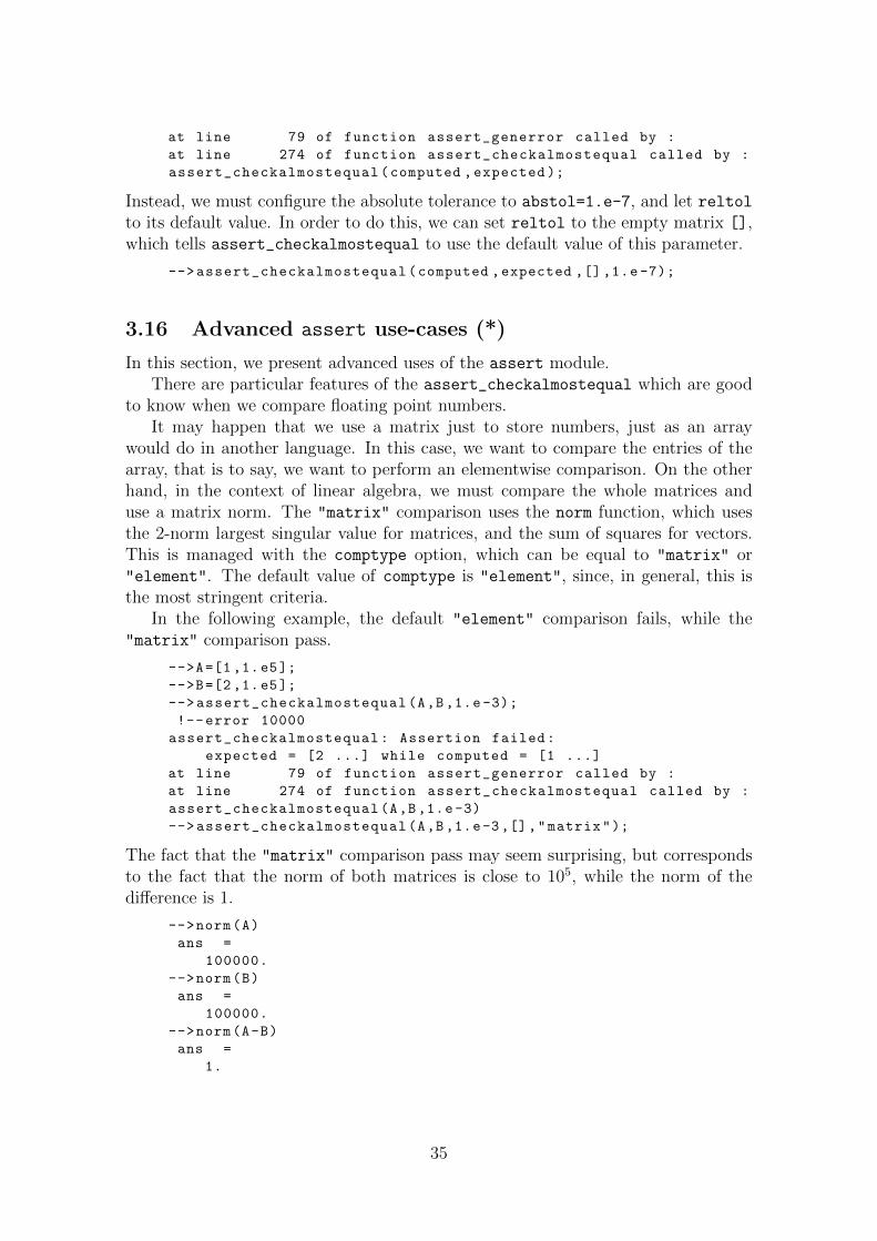
In this section, we present advanced uses of the assert module.There are particular features of the assert_checkalmostequal which are good
to know when we compare floating point numbers.It may happen that we use a matrix just to store numbers, just as an array
would do in another language. In this case, we want to compare the entries of thearray, that is to say, we want to perform an elementwise comparison. On the otherhand, in the context of linear algebra, we must compare the whole matrices anduse a matrix norm. The "matrix" comparison uses the norm function, which usesthe 2-norm largest singular value for matrices, and the sum of squares for vectors.This is managed with the comptype option, which can be equal to "matrix" or"element". The default value of comptype is "element", since, in general, this isthe most stringent criteria.
In the following example, the default "element" comparison fails, while the"matrix" comparison pass.
-->A=[1 ,1.e5];
-->B=[2 ,1.e5];
-->assert_checkalmostequal(A,B,1.e-3);
!--error 10000
assert_checkalmostequal: Assertion failed:
expected = [2 ...] while computed = [1 ...]
at line 79 of function assert_generror called by :
at line 274 of function assert_checkalmostequal called by :
assert_checkalmostequal(A,B,1.e-3)
-->assert_checkalmostequal(A,B,1.e-3,[],"matrix");
The fact that the "matrix" comparison pass may seem surprising, but correspondsto the fact that the norm of both matrices is close to 105, while the norm of thedifference is 1.
-->norm(A)
ans =
100000.
-->norm(B)
ans =
100000.
-->norm(A-B)
ans =
1.
35

Moreover, the function also takes into account for complex numbers, by compar-ing separately the real and imaginary parts. Special IEEE numbers such as %inf,%nan and signed zeros are also taken into account.
A particular feature of the module is that several of the assert functions havethe same output arguments. More precisely, all the functions in the Comparisonscategory of the figure 4 have the optional output arguments flag and errmsg, whereflag is true if the test pass (and false otherwise) and errmsg is an error message(which is the empty string "" if the test pass). This feature allows to get a uniformbehavior and supports a simple management of the errors in the case where anassertion is not satisfied.
For example, consider the function assert_checktrue, which calling sequenceis:
flag=assert_checktrue(condition)
flag=assert_checktrue(condition)
[flag ,errmsg ]= assert_checktrue(condition)
If any entry in condition is false,
• if the errmsg output variable is not used, an error is generated,
• if the errmsg output variable is used, no error is generated, the flag is set tofals and the errmsg variable is a string containing the error message.
The reason of this behavior is to be able to use assertions both in scripts (e.g. unittests) and in functions.
Let us illustrate this with an example. Within a unit test, the statement:
assert_checkequal (1+1 ,12);
will generate an error, as expected. On the other hand, consider the situation wherewe want to use assertions in a function. We might want to manage the case wherethe assertion fails. In this case, the function assert_checkequal generates an error,which interrupts the execution. We may want to avoid this, by catching the errorgenerated by assert_checkequal. To solve this problem, we may use the execstr
function, which leads to the following source code.
function y=myfunction(x)
ierr=execstr("assert_checkequal(x,12)","errcatch");
if ( ierr <> 0 ) then
error(msprintf("%s: Oups!","myfunction"))
end
y=x
endfunction
The following session presents two examples of the previous function.
-->myfunction (12)
ans =
12.
-->myfunction (24)
!--error 10000
myfunction: Oups!
at line 4 of function myfunction called by :
myfunction (24)
36
The previous function works, but is unnecessarily complex. Instead, we suggest touse the calling sequence
[flag ,errmsg ]= assert_checktrue(condition),
which simplifies the processing of the error. The following example presents a simpleuse of this calling sequence within a function.
function y=myfunction2(x)
[flag ,errmsg ]= assert_checktrue(x==12)
if ( ~flag ) then
error(msprintf("%s: %s","myfunction2",errmsg ))
end
y=x
endfunction
The following session presents an example of the myfunction2 function.
-->myfunction2 (24)
!--error 10000
myfunction2: assert_checktrue: Assertion failed:
found false entry in condition = F
at line 4 of function myfunction2 called by :
myfunction2 (24)
3.17 Generating the help from the macros
In general, any public function should be associated with an help page. This canlead to a considerable work when there are many functions in a module. In thissection, we present a method to automate the generation of help pages.
The content of the .xml file associated with the help page may be automaticallyproduced from the .sci file, thanks to the help_from_sci function. This functiongenerates the .xml file depending on the comments in the .sci file.
When we execute the help_from_sci function without input arguments, it opensthe editor with a template function, which comments can be customized.
help_from_sci ()
For example, the following mystery function contains comments which give adescription of the function.
function y = mystery ( x )
// Randomly performs a mysterious computation.
//
// Calling Sequence
// y = mystery ( x )
//
// Parameters
// x : a m-by -n, matrix of doubles
// y : a m-by -n, matrix of doubles , the output.
//
// Description
// Randomly computes results.
//
// Examples
// x = mystery ([1 2 4 5])
37

//
// Authors
// Bill Smith , 2010
x = x(:)
y = grand(1,"prm",x)
endfunction
In the previous function, the special keywords ”Calling Sequence”, ”Parame-ters”, ”Description”, ”Examples” and ”Authors” are automatically recognized bythe help_from_sci function, which creates the associated sections in the .xml file.In this case, the following statement would automatically generate the associatedhelp/en_US/ mystery.xml file, based on the macros/ mystery.sci file.
help_from_sci("macros","help/en_US")
A more complete solution is to use the helptbx module to automate the processof updating the .xml files of a module based on the .sci files. This script sequentiallyuses the help_from_sci function to automatically generate the .xml from the .sci
files in one given directory. Moreover, the .xml files can be automatically updateddepending on the time stamp of the .sci files. This is convenient in the cases wherewe update the comments in the .sci file during the development of the module.
As an example, we can analyse how the help pages of the number module werecreated. In the help/en_US directory of the module, the update_help.sce scriptupdates the .xml help pages from the .sci macros. The helptbx_helpupdate
function takes as input argument a matrix of strings defining the functions to update,the help directory and the macros directory.
helpdir = get_absolute_file_path("update_help.sce");
funmat = [
"number_carmichael"
"number_coprime"
"number_extendedeuclid"
[...]
];
macrosdir = cwd +"../../ macros";
demosdir = [];
modulename = "number";
helptbx_helpupdate(funmat ,helpdir ,macrosdir ,..
demosdir ,modulename ,%t);
When we execute the previous script, it prints the following output.
-->exec C:\ number\help\en_US\update_help.sce;
Working dir = C:\ number\help\en_US\
Updating number
Processing C:\ number\help\en_US \..\..\ macros\number_carmichael.sci
Processing C:\ number\help\en_US \..\..\ macros\number_extendedeuclid.sci
Processing C:\ number\help\en_US \..\..\ macros\number_coprime.sci
XML Changed C:\ number\help\en_US\number_coprime.xml
[...]
As we can see, the content of the number_coprime.sci file has changed, so thatthe associated .xml has to be updated. Since the other files have not changed, theassociated .xml files remains unchanged.
More informations on this topic are available in the help of the helptbx module:
38

http://atoms.scilab.org/toolboxes/helptbx
A specific work related to the help pages is the design of the examples. Moredetails on this topic are presented in the section 6.
3.18 Using pseudomacros (*)
In the case where we have to create the help pages of functions based on gateways(in the C language, for example), then the previous method cannot be used directly.In this case, a possible solution is to create pseudo-macros as .sci files, which onlycontain the comments necessary for the helptbx module.
For example, the accsum module is partly based on gateways. This module isavailable on the Forge at:
http://forge.scilab.org/index.php/p/accsum
The help/en_US/ pseudomacros directory contains a set of .sci files which onlycontains comments: the body of the function is empty, since the actual imple-mentation is done in the C gateways. These .sci files are used in the associatedupdate_help.sce script, which automatically generates the .xml files from the pseu-domacros.
3.19 A check-list for the module
The following list presents some checks that we may use to verify that our moduleis ready for a release.
• Does the module build ?
• Does the module load ?
• Do the unit tests pass ?
• Are the help pages correct ?
• Do the demos execute ?
4 Interfaces (*)
In this section, we describe various methods to let Scilab call a function which isexternal to Scilab. We consider a simple situation where a function is defined as amacro. This situation is used an example, so that we can use three different methodsto make the computation.
We first assume that the external software is provided as a binary executable,and we communicate with it by exchanging data files. In the third section, wedynamically compile and load a C function, and compute the function value withthe call statement. In the final section, we make a gateway toward a C functionand use it as if it was a built-in Scilab function.
39

4.1 Overview
We assume that the simulator is a function f defined by
y = f(x,p), (1)
where
• x ∈ Rnx is a real vector of size nx ≥ 1, which represents the input,
• p ∈ Rnp is a real vector of size np ≥ 1, which represents the parameters,
• y ∈ Rny is a real vector of size ny ≥ 1, which represents the output.
For example, the simulator can be a 3 dimensionnal fluid simulator of the flow in apipe, a finite element model of a bridge or a trajectory software for a spatial vehicle.
In many practical situations, the function f which is used in the numerical sim-ulation is not provided as a macro (or a set of macros), but is an independentsimulator which is completely external to Scilab. For example, the simulator maybe provided
• as a C/C++ or Fortran source code,
• as a binary library (such as a .dll on MS Windows, or a .so on GNU/Linux),
• as an executable which reads an input data file and write an output data file.
Obviously, the Scilab macro is the simplest simulator possible, because it allowsto manage the simulator very easily, using all the tools available to the Scilab de-velopper. Still, in some cases, it is not possible to re-develop the simulator into theScilab language. The following is the list of the two most common reasons for thisissue.
• In the case where the source code implementing the simulator is too large, itwould require too much time to re-develop the software. It is common thatthese tools are associated with hundred of thousands (or more) source codelines and required decades of work by dozens of developers.
• The simulator may not be available in source form, but only in binary form.This is often the case where we buy a scientific library or software from acommercial vendor.
• The performance of the same code in the Scilab language would be unpractical.This is the case, for example, when the algorithm cannot be vectorized. Ofcourse, the vectorization of the algorithm guarantees that the code is entirelyexecuted by a C or Fortran compiled source code, so that the performanceis the best possible in many situations. Moreover, Scilab may use optimized(e.g. multithread) libraries, so that a naive C implementation may be muchslower than Scilab. More details on this topic are presented in the section”Performance” of [3]. However, there are algorithms which cannot be vector-ized, because they are strongly iterative. In this case, a solution is to make aninterface to a compiled source code which performs the same algorithm.
40

In this situation, we need to be able to drive the external software and thissection presents several methods to do so. In order to make the presentation simple,we begin by describing a simple macro which represents the simulator f .
The examples provided in this section assume that we have access to a C compiler.Under Windows, we use Visual C 2010 while under Linux we use gcc version 4.0 orlater.
4.2 A sample function
For the sake of simplicity, we have chosen a extremely reduced model, which allowsto present the complete source codes. We consider here the Ishigami and Hommafunction [9] is often used as a benchmark for sensitivity analysis. We assume thatwe have nx = 3 input variables, np = 2 parameters and we want to compute thefunction
y = f(x,p) = sin(x1) + p1 sin(x2)2 + p2 sin(x1)x
43, (2)
where x ∈ R3, p ∈ R2 and y ∈ R. The following function implements the simulator.
function y = ishigami ( x , p )
a = p(1);
b = p(2);
s1=sin(x(1));
s2=sin(x(2));
y(1) = s1 + a*s2^2 + b*s1*x(3)^4;
endfunction
In the following session, we call the simulator with x = (1, 2, 3) and p = (7, 0.1).
-->x = [1 2 3];
-->p = [7. 0.1];
-->format (25);
-->y = ishigami ( x , p )
y =
13.44513863477450144046
The exact result for this computation has been computed by Wolfram Alpha,thanks to the expression sin(1)+7*sin(2)^2+1/10*sin(1)*3^4. The exact resultis
13.445138634774499911774859767677847231549791441526940562146
which is accurate to the displayed digits. The relative error for this computation is8.09382 · 10−17, which corresponds to the expected accuracy for a double precisioncomputation.
4.3 By files
In this section, we analyze a straightforward implementation of the call from Scilabto an external executable, where the data is exchanged by files. We emphasizeprecision issues related to the floating point representation of Scilab floating pointnumbers.
We consider that we are given an executable which implements our simulator fand which
41

• reads an input data file,
• makes its computation,
• writes an output data file.
It may seem, at first, that exchanging data by files is both too basic and ineffi-cient.
Indeed, the transfer rate between the memory and a typical hard drive is slow,compared to the transfer rate inside the memory. Still, there are pratical situa-tions where the CPU time required by the simulator to perform its computationis greater than 1 minute, and it is not rare that a 3 dimensionnal fluid simulationrequires hours or even days of computations, even with parallel algorithms. In thesesituations, the costs of reading and writing the data is negligible. Obviously, if thesimulation requires less than 1 second, the question needs to be discussed more pre-cisely, including the time required by the system to create the associated process.Anyway, the performance issue should be analyzed with respect to the orders ofmagnitude of the times involved in the particular simulation.
Another issue is the formatting of the files into a language which can be easilyread by the simulator. For example, this language might be particular to spatialmission analysis, to a oil reservoir simulation tool or an .xml data file. In our case, wewill design an external simulator which reads and write simple text files. We couldargue that this will require binary to decimal conversions, which can be inaccurate.Instead, we could use binary files, so that no conversion is performed, which shouldensure a better accuracy. For example, we could use the HDF file format [7] tostore our data as a binary portable data file. When there is a lot of datas to store,text files can be larger than binary files. Still, in practice, binary files are less easyto manage than text files. Indeed, we must use a program to read the binary file,instead of directly reading the file. This is why many scientific programs still worksby exchanging basic text data files. This is the reason why we chose this methodfor our example, which results in a much simpler example.
In order to simplify the discussion, we assume that the external simulator canread and write a basic text data file, formatted with (key,value) pairs. Moreover,we assume that our simulation requires enough CPU time to make the data ex-change and the process creation negligible. Our external simulator will implementthe ishigami function in the C language. Although this computation is obviouslyvery fast, it may represent a complex simulation tool requiring hours of computation.
The input and output data files are presented in the figures 5 and 6. We em-phasize that the decimal to binary conversion for floating point numbers might leadto numerical issues. First, we notice that Scilab stores the real floating point num-bers with IEEE double precision, associated with 64 bits, where 52 bits are usedin the mantissa. Then, it is known that the algorithms which convert the decimalrepresentation of doubles into and from binary floating point numbers are tricky.We can prove that 17 decimal digits are required so that the decimal representationof the floating point number exactly correspond to the binary representation of thebinary floating number[13, 6]. That is, 17 decimal digits is the minimum numberof decimal digits so that a write-read cycle is error-free, when the conversions are
42

NX 3
X
1.00000000000000000e+000
2.00000000000000000e+000
3.00000000000000000e+000
NP 2
P
7.00000000000000000e+000
1.00000000000000010e-001
Figure 5: The input data file
NY 1
Y
1.34451386347745010e+001
Figure 6: The output data file
correctly rounded to nearest. This is why our input and output data files are using17 decimal digits precision. More details on floating point numbers in Scilab can befound in [1]
The following is the content of the source code ishigami.c. In order to use theprogram, we use the command ishigami inputfile.txt outputfile.txt in theterminal.
#include <math.h>
#include <stdio.h>
#include <stdlib.h>
void ishigami(int * nx , double * x, int * np ,
double * p, int * ny , double * y);
/* Usage:
ishigami inputfile.txt outputfile.txt */
int main(int argc , char *argv []) {
char * inputfn , * outputfn;
FILE *fd;
int nx, np, ny, i;
double * x, * p, * y;
char key [10];
if ( argc !=3 ) {
/* Check the number of input arguments */
printf("Wrong number of input arguments .\n");
printf("Usage: ishigami inputfile.txt outputfile.txt\n");
exit (0);
}
/* Get the input and the output files */
inputfn = argv [1];
outputfn = argv [2];
fd=fopen(inputfn ,"r"); /* Read the input file */
fscanf(fd,"%s %d",key ,&nx); /* Read NX */
fscanf(fd,"%s",key); /* Read X */
x = malloc ( nx * sizeof(double) );
43

for (i=0;i<nx;i++) {
fscanf(fd,"%lf",x+i);
}
fscanf(fd,"%s %d",key ,&np); /* Read NP */
fscanf(fd,"%s",key); /* Read P */
p = malloc ( np * sizeof(double) );
for (i=0;i<np;i++) {
fscanf(fd,"%lf",p+i);
}
fclose(fd);
ny = 1; /* Prepare ny, y */
y = malloc ( ny * sizeof(double) );
/* Call the function */
ishigami (&nx , x, &np , p, &ny , y);
/* Write output file */
fd=fopen(outputfn ,"w");
fprintf(fd ,"NY %d\n",ny);
fprintf(fd ,"Y\n");
for (i=0;i<ny;i++) {
fprintf(fd ,"%.17e\n",y[i]);
}
fclose(fd);
free(x); /* Clean -up */
free(p);
free(y);
}
void ishigami(int * nx , double * x, int * np ,
double * p, int * ny , double * y)
{
double a, b, s1, s2;
a = p[0];
b = p[1];
s1=sin(x[0]);
s2=sin(x[1]);
y[0] = s1 + a*s2*s2 + b*x[2]*x[2]*x[2]*x[2]*s1;
}
We now analyze the content of this program. The program first checks the valueof the variable argc, which contains the number of arguments, which is expectedto be equal to 3 (where the argument number 0 is the command name, that is,ishigami). Once this is done, we open the input data file associated with theinputfn variable. The first line contains the number of entries in the array x, whichis associated with the (key,value) pair NX 3. In the current program, we read thevalue 3 and ignore the key NX. In a more complete program, we should check thatthe key which has been read in the data file is equal to the string ”NX”. Then,we allocate the array x to the corresponding size nx. Notice that the x variable isdeclared as a double, which corresponds to the precision which is used by Scilab forthe real matrices. Hence, the precision of the simulator corresponds to the precisionof the floating point numbers used by Scilab. The key X is ignored and the entries ofthe variable x are read, one by one. We use the format ”%lf” for the reading, whichcorresponds to the double format. A similar method is applied for the p variable.Then, we set the variable ny to 1 and allocate the array y. The computation isperformed by the ishigami function, which implements the actual simulator f . We
44

emphasize that this function uses double variables, which exactly correspond to thedata type used by Scilab in its internal representation of floating point numbers.Once the output y of the simulator has been computed, we open the output file andwrite its content. We use the ”%.17e” format for the writing, so that 17 decimaldigits are used.
We compile this source code with usual tools. Under a Windows 32 bits system,we use Visual C++ 2008, where we declared the pre-processing variable
CRT SECURE NO WARNINGS
which allows to avoid the warning messages with respect to the unsafety of thefopen and fscanf functions. Under a Linux 32 bits system (Ubuntu), we use gccversion 4.4.1. We used the command gcc -lm ishigami.c -o ishigami.exe.
The following Scilab ishigami function takes as input arguments the input x,the parameter p, the name of the executable exename, the names of the input andoutput files infile and outfile and returns the output y. The ishigami functionwrites the input data file, calls the executable and reads the output data file. Weemphasize that, when the x variable is written, we use the ”%.17e” format, so that17 decimal digits are written in the input data file. Inversely, when we read the y
variable, we use the ”%lf” format, which corresponds to the double format.
// ishigami
// Compute the Ishigami function.
// Arguments:
// x : input , row matrix , size 3
// p : input , row matrix , size 2
// y : output , size 1
// infile : the name of the input file
// outfile : the name of the output file
function y = ishigami ( x , p , exename , infile , outfile )
nx = size(x,"c");
np = size(p,"c");
// Write the input data file
[fd,err] = mopen(infile , "w" );
mfprintf(fd ,"NX %d\n", nx);
mfprintf(fd ,"X\n");
for i=1:nx
mfprintf(fd ,"%.17e\n",x(i));
end
mfprintf(fd ,"NP %d\n", np);
mfprintf(fd ,"P\n");
for i=1:np
mfprintf(fd ,"%.17e\n",p(i));
end
mclose(fd);
// Call the isghigami.exe executable
cmd = msprintf("%s %s %s",exename , infile , outfile );
stat = unix ( cmd );
if ( stat ==1 ) then
mprintf ("Failed to launch executable.")
end
// Read the output data file
[fd,err] = mopen(outfile , "r" );
45

[ny , key] = mfscanf(fd,"%s %d");
key = mfscanf(fd,"%s");
for i=1:ny
y(i)= mfscanf(fd,"%lf\n");
end
mclose(fd);
endfunction
In order to launch the executable, we have used the unix function. Despite itsname, this function works equally under Linux or Windows operating systems. Theoutput argument stat is equal to 0 if the call performed without error and is equalto 1 if there was an error.
There might be some problems at this stage of the development process. Forexample, there might be a bug in our formats, so that the input or output data filesmight be wrong. In this case, it is convenient to separately launch the Scilab macroor the executable and to check the data file. Some error messages might be writtenin the terminal. Under Linux, we can look at the terminal where Scilab has beenlaunched. Under Windows, we can use the statement
consolebox("on");
which opens the terminal associated with the current Scilab session. In order toclose this concole, we use the statement
consolebox("off");
In the following script, we use the function ishigami in order to compute theoutput of the simulator.
x = [1 2 3];
p = [7. 0.1];
exename = "ishigami.exe";
infile = "input.txt";
outfile = "output.txt";
format (25);
y = ishigami ( x , p , exename , infile , outfile )
The following session presents the result under Windows.
-->y = ishigami ( x , p , exename , infile , outfile )
y =
13.44513863477450144046
The following session presents the result under Linux.
-->y = ishigami ( x , p , exename , infile , outfile )
y =
13.445138634774499664104
We notice that there is a slight discrepancy between the results produced by theprogram under Linux and Windows. The relative error for the Windows result is8.09382 · 10−17 while the relative error for the Linux result is 1.57510 · 10−17. Thereare many possible explanations for this numerical difference [4]. Since the relativeerror of both results correspond to the expected precision of double precision floatingpoint numbers, we consider that both results are consistent and accurate enough.
46

4.4 With the call function
In this section, we use the call function in order to compute the Ishigami andHomma function, provided as a C function.
4.4.1 The C source code
The following C function, stored in the ishigami.c file, implements the Ishigamifunction.
#include <math.h>
void ishigami(int * nx , double * x, int * np , double * p,
int * ny , double * y)
{
double a, b, s1, s2;
a = p[0];
b = p[1];
s1=sin(x[0]);
s2=sin(x[1]);
y[0] = s1 + a*s2*s2 + b*x[2]*x[2]*x[2]*x[2]*s1;
}
We can compile the C source code with Scilab with the ilib_for_link function,as in the following script.
ilib_for_link("ishigami","ishigami.c" ,[],"c");
The first argument of ilib_for_link, i.e. "ishigami" is the name of the symbolwhich is to be created. The second argument, "ishigami.c" is the name of thefile which contains the C source code. We skip the third argument with an emptymatrix [] and we set the fourth argument "c", which corresponds to the languagethat we use (we would have set ”f” for a fortran source code). The ilib_for_link
function creates various files behind the scenes. When everything happens correctly,the following output is produced, for example under Windows.
-->ilib_for_link(’ishigami ’,’ishigami.c’,[],"c");
Generate a loader file
Generate a Makefile
Running the Makefile
Compilation of ishigami.c
Building shared library (be patient)
Generate a cleaner file
Scilab has produced a dynamic library (called libishigami.dll under Windowsand libishigami.so under Linux) which can be loaded into Scilab. Scilab has alsoproduced a loader script, called loader.sce, which contains statements to load thedynamic library. In the following session, we execute the loader script, which loadsthe dynamic library into Scilab.
-->exec loader.sce;
Shared archive loaded.
Link done.
47

4.4.2 Debugging with ilib_for_link
In general, it takes some time to setup a working set of files and options so thatilib_for_link can finally work. When something wrong happens, as in the follow-ing session, we usually have little information about the actual problem, as shownin the following session under Windows, where we have written something wrong inthe source code of ishigami.c.
-->ilib_for_link(’ishigami ’,’ishigami.c’,[],"c")
Generate a loader file
Generate a Makefile
Running the Makefile
Compilation of ishigami.c
Building shared library (be patient)
NMAKE : fatal error U1077: ’"C:\ Program Files\Microsoft
Visual Studio 9.0\VC\bin\cl.EXE"’ : return code ’0x2 ’
Stop.
!--error 10000
unix_s: error during "nmake /Y /nologo /f Makelib.mak all"
execution
at line 34 of function unix_s called by :
at line 67 of function ilib_compile called by :
at line 59 of function ilib_for_link called by :
ilib_for_link(’ishigami ’,’ishigami.c’,[],"c")
In this situation, the debugging method depends on the operating system. In allcases, we must manually launch the Makefile generated by Scilab.
Under Windows, we can begin by opening a terminal with the following state-ment, which launches the start program built in MS Windows.
unix start
The previous statement opens a particular terminal, where all the environment as-sociated with Scilab has been configured. Then, we can launch the makefile with thenmake command, as in the following session, which is performed inside MS Windows’terminal.
F:\usecall >nmake /f Makelib.mak
Microsoft (R) Program Maintenance Utility Version 9.00.21022.08
Copyright (C) Microsoft Corporation. All rights reserved.
------------- Compile file ishigami.c --------------
IF NOT EXIST Debug mkdir Debug
cl -D__MSC__ -DFORDLL -DWIN32 -c [...] ishigami.c
ishigami.c
ishigami.c(6) : error C2065: ’a’ : undeclared identifier
ishigami.c(6) : warning C4244: ’=’ : conversion from ’double ’
to ’int ’, possible loss of data
ishigami.c(10) : error C2065: ’a’ : undeclared identifier
NMAKE : fatal error U1077: ’"C:\ Program Files\Microsoft
Visual Studio 9.0\VC\bin\cl.EXE"’ : return code ’0x2 ’
Stop.
F:\usecall >
We see that the variable ”a” has not been declared. It is then easy to fix the bugand to finally compile the code. It may happen that we get the following message inMS Windows terminal, which states that the dynamic library could not be opened.
48
Creation of dll libishigami.dll and import lib from ...
ishigami.obj
LINK : fatal error LNK1104: cannot open file ’libishigami.dll ’
This happens when the library has already been loaded into Scilab, may be aftera successful compilation. If we modify the source code and compile it again, thecompiler cannot access to the library, because it is already loaded, so that the file islocked. This is why it is always safe to unload all the previously libraries with theulink function, before loading it again, as in the following session.
ulink ();
ilib_for_link("ishigami","ishigami.c" ,[],"c");
exec loader.sce;
The following is the output of the ilib_for_link function under Linux.
-->ilib_for_link("ishigami","ishigami.c" ,[],"c")
Generate a loader file
Generate a Makefile
ilib_gen_Make: configure : Generate Makefile.
ilib_gen_Make: Copy compilation files (Makefile*, libtool ...)
to TMPDIR
ilib_gen_Make: Copy ishigami.c to TMPDIR
ilib_gen_Make: Modification of the Makefile in TMPDIR.
Running the Makefile
Generate a cleaner file
We see that Scilab copies the files into the temporary directory before actuallycompiling them. We now consider a case where the source code in ishigami.c
contains an error. In this case, Scilab produces the following output.
-->ilib_for_link("ishigami","ishigami.c" ,[],"c")
Generate a loader file
Generate a Makefile
ilib_gen_Make: Copy compilation files (Makefile*, libtool ...)
to TMPDIR
ilib_gen_Make: Copy ishigami.c to TMPDIR
ilib_gen_Make: Modification of the Makefile in TMPDIR.
Running the Makefile
ilib_compile: An error occured during the compilation:
!ishigami.c:2: error: expected ’)’ before ’*’ token !
!make: *** [ishigami.lo] Error 1 !
Generate a cleaner file
We first get the value of the TMPDIR variable from Scilab’s console.
-->TMPDIR
TMPDIR =
/tmp/SD_2277_
Now that we know where the temporary directory is, we open a Linux terminal, goto this directory and get the list of files in this directory.
/tmp/SD_2277_$ cd /tmp/SD_2277_
/tmp/SD_2277_$ ls
aclocal.m4
configure
configure.ac
ishigami.loT
49
ishigami.c
libishigami.la
libtool
Makefile.am
Makefile.in
Makefile.orig
Makefile
We see that the ishigami.c source code has been copied there, along the Makefilewhich has been automatically created by Scilab. We can launch the Makefile whichmakes the following messages appear in the terminal.
myname@desktop :/tmp/SD_2277_$ make
/bin/bash ./ libtool --tag=CC --mode=compile gcc -I. -g -O2 -g
-O2 -c -o ishigami.lo ishigami.c
gcc -I. -g -O2 -g -O2 -c ishigami.c -fPIC -DPIC
-o .libs/ishigami.o
ishigami.c:2: error: expected ’)’ before ’*’ token
make: *** [ishigami.lo] Error 1
We can then fix the source code in the original directory (not in the temporarydirectory) and launch the ilib_for_link function until the bug is fixed.
4.4.3 Using call
We assume that the ishigami.c has been correctly compiled by ilib_for_link sothat the loader script was able to load the library into Scilab.
The following ishigami function implements a Scilab macro, which computesthe Ishigami function by using the call function. The ishigami function takes theinput row matrices x and p and returns the output argument y.
function y = ishigami ( x , p )
nx = size(x,"c");
np = size(p,"c");
ny = 1;
y = call("ishigami",nx ,1,"i",x,2,"d",np ,3,"i" ,..
p,4,"d",ny ,5,"i","out" ,[1,ny],6,"d");
endfunction
In the previous function, we used the size function to compute the size number ofcolumns of the input arguments x and p. We also used the call function in orderto use the dynamic library that we loaded earlier in this section.
The call function allows to call a Fortran or C user program from Scilab. Itssyntax is the following.
[y1 ,...,yk]=call("ident",x1,px1 ,"tx1" ,...,xn,pxn ,"txn" ,...
"out",[ny1 ,my1],py1 ,"ty1" ,...,[nyl ,myl],pyl ,"tyl")
The input arguments of the call function are a defining the specification of thearguments of the routine. The first input argument of the call function, that is”ident” in our example, is a string which represents the name of the routine. Then,we must pass sequences of three arguments (x1,px1,tx1), which define the inputarguments of the routine. Each set (x1, px1, tx1) has the following sense:
• x1 is the input argument which is passed to the routine,
50

”r” float”i” int”d” double”c” string
Figure 7: C data types for the call function.
• px1 is an integer representing the position of the input argument (i.e. 1, 2, 3,etc...),
• tx1 is a string representing the type of the input argument.
The figure 7 presents the various data types which are available with the call
function.The "out" string is a mark for the begining of the output variable specification.
We must pass sequences of three arguments ([ny1,my1],py1,ty1) which define theoutput arguments of the routine. Each set ([ny1,my1],py1,ty1) has the followingsense:
• [ny1,my1] is the shape of the matrix associated with the output argumentand ny1 and my1 are positive integers,
• py1 is an integer representing the position of the output argument (i.e. 1, 2,3, etc...),
• ty1 is the type of the output argument.
In our example, we first consider the header of our C function ishigami:
#include <math.h>
void ishigami(int * nx , double * x, int * np , double * p,
int * ny , double * y)
We see that the function takes 6 arguments, where we assume that the arguments1 to 5, i.e. nx to ny, are input arguments and the argument number 6, i.e. y, is theoutput argument. The figure 8 presents the map from the call argument to the Csource code. This leads to the following call statement, where we have expandedthe statements on several lines to make it more clear:
y = call("ishigami" ,..
nx ,1,"i" ,..
x,2,"d" ,..
np ,3,"i" ,..
p,4,"d" ,..
ny ,5,"i" ,..
"out" ,..
[1,ny],6,"d");
The following script shows how to use the ishigami function.
format (25)
x = [1 2 3];
p = [7. 0.1];
y = ishigami ( x , p )
51

Position Type C source code Argument of call
1 input int * nx nx,1,"i"
2 input double * x x,2,"d"
3 input int * np np,3,"i"
4 input double * p p,4,"d"
5 input int * ny ny,5,"i"
6 output double * y [1,ny],6,"d"
Figure 8: Map from the C source code to the call arguments.
Data
Type
Number of rows
Number of columns
IsReal
Header
Figure 9: Structure of a matrix of doubles.
4.5 With a gateway
In this section, we present the method which is used by Scilab developers to createan interface to a library. This type of interface is called a gateway in the contextof Scilab and corresponds to the closest link which can be designed between Scilaband an external library.
4.5.1 Scilab data structures
In order to analyze a gateway, we must first analyze the way that variables aremanaged by Scilab. The figure 9 presents the structure of a matrix of doubles,which is one of the most common data types in Scilab.
Any variable in Scilab is made of a header, which specifies some data. The headeris made of one or more fields. The first field is an integer which identifies the type ofcontent of the matrix. The various values of this field correspond to the various datatypes which are available in Scilab. The map from Scilab types to integer values arepresented in figure 10.
When the variable is a sci matrix, the next fields are the number of rows, thenumber of columns and a boolean which indicates if the matrix contains complexvalues. If the matrix contains real values only, then the data is made of an array ofdouble. If the matrix contains complex values, then two arrays are used, the first
52
Data type Value Data type Valuesci matrix 1 sci u function 11sci poly 2 sci c function 13sci boolean 4 sci lib 14sci sparse 5 sci list 15sci boolean sparse 6 sci tlist 16sci matlab sparse 7 sci mlist 17sci ints 8 sci pointer 128sci handles 9 sci implicit poly 129sci strings 10 sci intrinsic function 130
Figure 10: Map from the C data type name to the integer value.
A11
A21
Am1...
A11
A21
Am1
...
...
A11
A21
Am1
...
Figure 11: Order of the values in a matrix of doubles.
for the real part and the second for the imaginary part.Consider a matrix of doubles with m rows and n columns and real values only.
The values in the array are stored column-by-column, as presented in the figure 11.This corresponds to the order of the matrices in the Fortran language. This facthas not been chosen by chance. It corresponds to the fact that the underlying linearalgebra libraries which are used by Scilab are from the Lapack project, where thesource code is in the Fortran language.
4.5.2 The Scilab API
Assume that we want to design a function ishigami associated with the followingcalling sequence:
y = ishigami ( x , p )
In the following we analyze the management of the input arguments x and p in theright hand side (called RHS in the gateways) and the output argument y (calledLHS in the gateways). When we implement the gateway, we perform the followingsequence of actions :
• read the input argument number 1, named x, and check its type and size (i.e.
53

CheckColumn checks if a parameter is a column vectorCheckDimProp checks the compatibility between 2 argumentsCheckDims checks if a parameter has the required dimensionsCheckLength checks the length of a vectorCheckLhs checks the number of output argumentsCheckRhs checks the number of input argumentsCheckRow checks if a parameter is a row vectorCheckSameDims checks if two parameters have the same sizeCheckScalar checks if a parameter is a scalarCheckSquare checks if a parameter is a square matrixCheckVector checks if a parameter is a vector (column or row)Scierror displays an error message to the usersciprint displays standard messages to the user
Figure 12: General purpose functions of the API Scilab.
its number of rows and columns),
• read the input argument number 2, named p, and check its type and size (i.e.its number of rows and columns),
• allocate the output argument number 1, a matrix of doubles named y,
• call the ishigami function, which writes the content of the y variable.
For each action in the gateway we will call one or several C functions whichare provided by the Scilab C Application Programming Interface (API). Indeed,Scilab v5.2 provides a complete C API which is both consistent and powerful. Thedocumentation for this API is included in the inline help of Scilab, in the ”APIScilab” section. Several general purpose functions of this API are presented in figure12. Some functions related to the management of matrices of doubles are presentedin figure 13.
This API is powerful and cannot be covered completely in this document. In-stead, we chose to focus on the simple management of double matrices, so that wecan get a practical understanding of the matrix of doubles.
4.5.3 Analysis of a gateway
We now analyze the main lines of the source code of the sci_ishigami gateway.The first lines of source code are devoted to the inclusion of the required headers.
#include "stdlib.h"
#include "stack -c.h"
#include "api_scilab.h"
#include "Scierror.h"
#include "localization.h"
The following C source code is the header of the gateway.
int sci_ishigami (char *fname) {
54

getMatrixOfDouble()Get the address of the values of a matrix of double
getComplexMatrixOfDouble()Get the address of the values of a complex matrix of double
createMatrixOfDouble()Create the address from an existing matrix of double
createComplexMatrixOfDouble()reate the address from an existing complex matrix of double
allocMatrixOfDouble()Create the address of a new matrix of double
allocComplexMatrixOfDouble()Create the address of a new complex matrix of double
Figure 13: Functions of the API Scilab to manage matrix of doubles. – The get
functions allow to read the input arguments. The create and alloc functions allowto write the output arguments.
The fname variable contains the name of the function, that is, contains the string"ishigami".
In the first lines of the gateway, presented in the following C source code, wecall the CheckRhs and CheckLhs functions to make sure that the user provided thecorrect number of input and output arguments.
CheckRhs (2,2);
CheckLhs (0,1);
When the user does not provide the correct number of input arguments, an error isgenerated, as in the following session.
-->y = ishigami ( x , p , x )
!--error 77
ishigami: Wrong number of input argument(s): 2 expected.
We now read the input argument x. This corresponds to the following simplifiedsequence of calls.
sciErr=getVarAddressFromPosition(pvApiCtx ,1,& piAddr );
sciErr=getVarType(pvApiCtx ,piAddr ,&iType);
sciErr=getMatrixOfDouble(pvApiCtx ,piAddr ,&nRowsX ,&nColsX ,&x);
We first call the getVarAddressFromPosition function and tell the function thatwe want to get the adress of the input argument #1. As a result, we get the value ofthe integer piAddr variable, which contains the adress of the variable. This adressallows to locate the structure corresponding to the variable in Scilab’s memory androughly corresponds to the whole content of the figure 9, including the header andthe data. Then, we analyze the header and call the getVarType in order to get thetype of input variable in the integer iType. Finally, we call the getMatrixOfDouble
and get the number of rows nRowsX, the number of columns nColsX and the arrayof doubles x.
Each function returns a data structure sciErr, which contains a nonzero field ifthere is an error.
55

if(sciErr.iErr)
{
printError (&sciErr , 0);
return 0;
}
If there is an error, the gateway calls the printError function in order to print anerror message in the console.
The following block of source code corresponds to the case where the inputargument #1 is no a matrix of double. In this case, we call the Scierror functionin order to generate an error message. The underscore sign _ before the string allowsto call a function which translates the string into a localized message, i.e., a messagewhich corresponds to the language configured on the machine.
if(iType != sci_matrix)
{
Scierror (204,_(
"%s: Wrong type for input argument #%d: Matrix expected .\n"),
fname ,1);
return 0;
}
This situation is presented in the following session, where we pass a string insteadof a matrix of doubles.
-->y = ishigami ( "foo" , "foo" )
!--error 204
ishigami: Wrong type for input argument #1: Matrix expected.
In the following C source code, we call the CheckDims function in order to checkthat the input argument #1 is a row matrix, with 1 row and 3 columns.
CheckDims(1,nRowsX ,nColsX ,1 ,3);
In the following Scilab session, we see that if a row matrix with 4 entries is passedo the ishigami function, an error message is generated.
-->y = ishigami ( [1 2 3 4] , p )
!--error 999
ishigami: first argument has wrong dimensions (1,4),
expecting (1,3).
The same operations must be performed for the second argument, so that wefinally get the vector p.
We now allocate a matrix of doubles so that we can later write into the y array.For this purpose, we call the allocMatrixOfDouble function and create the outputvariable, identified by the integer Rhs+1 in Scilab’s memory.
nRowsY =1;
nColsY =1;
sciErr=allocMatrixOfDouble(pvApiCtx ,Rhs+1,nRowsY ,nColsY ,&y);
If we had to create an output variable #2, we would pass the value Rhs+2 instead.We can finally call the ishigami function, as in the following C source code.
ishigami (& nColsX , x, &nColsP , p, &nColsY , y);
The last line before the end of the gateway is presented in the following C sourcecode. It allows to tell Scilab that the output argument #1 is located at index Rhs+1.
56

LhsVar (1) = Rhs+1;
If we had to create an output variable #2, we would write LhsVar(2) = Rhs+2
instead.The following source code is the content of the sci_ishigami.c file which im-
plements the gateway.
#include "stdlib.h"
#include "stack -c.h"
#include "api_scilab.h"
#include "Scierror.h"
#include "localization.h"
int sci_ishigami (char *fname);
void ishigami(int * nx , double * x, int * np , double * p,
int * ny , double * y);
// y = ishigami ( x , p )
// Computes the Ishigami function
int sci_ishigami (char *fname) {
double * x;
double * p;
double * y;
int nRowsX , nColsX;
int nRowsP , nColsP;
int nRowsY , nColsY;
SciErr sciErr;
int *piAddr = NULL;
int iType = 0;
CheckRhs (2,2) ;
CheckLhs (0,1) ;
// Get 1st argument : x
sciErr = getVarAddressFromPosition(pvApiCtx , 1, &piAddr );
if(sciErr.iErr)
{
printError (&sciErr , 0);
return 0;
}
sciErr = getVarType(pvApiCtx , piAddr , &iType);
if(sciErr.iErr)
{
printError (&sciErr , 0);
return 0;
}
if(iType != sci_matrix)
{
Scierror (204,_(
"%s: Wrong type for input argument #%d: Matrix expected .\n"),
fname ,1);
return 0;
}
sciErr=getMatrixOfDouble(pvApiCtx ,piAddr ,&nRowsX ,&nColsX ,&x);
if(sciErr.iErr)
{
printError (&sciErr , 0);
return 0;
}
CheckDims(1,nRowsX ,nColsX ,1 ,3);
57

// Get 2nd argument : p
sciErr = getVarAddressFromPosition(pvApiCtx , 2, &piAddr );
if(sciErr.iErr)
{
printError (&sciErr , 0);
return 0;
}
sciErr = getVarType(pvApiCtx , piAddr , &iType);
if(sciErr.iErr)
{
printError (&sciErr , 0);
return 0;
}
if(iType != sci_matrix)
{
Scierror (204,_(
"%s: Wrong type for input argument #%d: Matrix expected .\n"),
fname ,2);
return 0;
}
sciErr=getMatrixOfDouble(pvApiCtx ,piAddr ,&nRowsP ,&nColsP ,&p);
if(sciErr.iErr)
{
printError (&sciErr , 0);
return 0;
}
CheckDims(2,nRowsP ,nColsP ,1 ,2);
// Create output argument y in Scilab
nRowsY = 1;
nColsY = 1;
sciErr=allocMatrixOfDouble(pvApiCtx ,Rhs+1,nRowsY ,nColsY ,&y);
if(sciErr.iErr)
{
printError (&sciErr , 0);
return 0;
}
// Compute y
ishigami (& nColsX , x, &nColsP , p, &nColsY , y);
// Let Scilab know that Rhs + 1 is the 1st
// (and only) output argument
LhsVar (1) = Rhs+1;
return 0;
}
void ishigami(int * nx , double * x, int * np , double * p,
int * ny , double * y)
{
double a, b, s1, s2;
a = p[0];
b = p[1];
s1=sin(x[0]);
s2=sin(x[1]);
y[0] = s1 + a*s2*s2 + b*x[2]*x[2]*x[2]*x[2]*s1;
}
The following script is the builder.sce script.
gateway_path = get_absolute_file_path("builder.sce");
58

libname = "ishigamigateway";
namelist = [
"ishigami" "sci_ishigami"
];
files = [
"sci_ishigami.c"
];
ldflags = "";
libs = [];
tbx_build_gateway(libname , namelist , files , gateway_path , ..
libs , ldflags , cflags );
clear tbx_build_gateway;
The builder.sce script uses the tbx_build_gateway function in order to compilethe gateway.
The following shows how to use execute the builder, load the dynamic libraryand call the ishigami function.
exec builder.sce;
exec loader.sce;
x = [1 2 3];
p = [7. 0.1];
y = ishigami ( x , p )
4.5.4 Debugging a gateway
It is clear that developping a gateway requires some knowledge of how to compilea program. Nevertheless, some resources are provided in order to make the processmuch easier. The Scilab wiki pages [5, 10] present methods in order to debug Scilabunder Windows and Linux.
On Windows, we may use MS Visual Studio, for example, in order to interactivelydebug the gateway. In order to generate a debug version of the binary, we must setthe DEBUG_SCILAB_DYNAMIC_LINK environment variable to the ”YES” value, whichenables the debug switches of the compiler. The MS Windows operating systemallows to create environment variables through various dialog boxes in the SystemProperties dialog. We can also use the setenv function, as in the following session.
-->setenv("DEBUG_SCILAB_DYNAMIC_LINK","YES")
Once this variable is created, we can launch the builder script and load the library.Finally, we can run MS Visual Studio and connect it to the Scilab binary. This can bedone with the ”Debug> Attach to Process ...”dialog box of MS Visual Studio. Then,we select the ”WScilex.exe” process, which makes the debugger load the dynamiclibraries associated with Scilab. We can then put a breakpoint in the gateway anddebug it interactively.
If the binary we use is a regular, optimized, binary (as one that we have down-loaded from the website), we will be able to debug our gateway, but we will not beable to make interactive steps inside Scilab’s source code. Most of the time, thisdoes not prevent from making very fast progress toward a bug fix. In more complexcases, we need to compile Scilab from the sources, which allows to make interactivesteps in Scilab’s source code.
59
On Linux, we can use gdb or a front-end such as Kgdb to debug the gatewayinteractively. The Scilab main script accept the -debug switch, as in the followingcommand, which is called from the Linux terminal
bin/scilab -debug
The previous command runs Scilab in debug mode under gdb.Whatever the operating system we use, it is not rare that developping new gate-
ways require hours of analysis and bug finding. In this case, we can ask for help inthe various Scilab forums which are designed for this purpose. In this context, anefficient way of communicating is to simplify the source code as much as possibleand to provide a sample script which
4.6 A module with gateways
In this section, we present a module which uses gateways to provide functions basedon a compiled source. In the first part, we present the src directory and then thesci_gateway directory.
To illustrate this section, we use the NISP module that we have used in thesection 2.3. The sources of the module can be downloaded from ATOMS, or fromthe Forge, where the module is developped:
http://forge.scilab.org/index.php/p/nisp/
4.6.1 The src directory
The src directory contains the sources of the library that we want to interface.In general, the name of the src subdirectories should be related to their content:
• src/f, if the code contains a set of Fortran 77 source codes,
• src/c, if the code contains a set of C source codes.
• src/cpp, if the code contains a set of C++ source codes.
But this general rule is flexible, since the actual name can be chosen freely, as weare going to see.
In the case of the NISP module, the src directory contains the sources of theNISP C++ library, and its dependencies. The following is the list of the files andsub-directories which are typically found in this directory.
• NISP/src/builder_src.sce: the builder of the sources. This script launchesthe compilation of the sources.
• NISP/src/cleaner_src.sce: the cleaner of the sources. This script deletesthe files which are generated by the compilation.
• NISP/src/includes: the headers .h of the library. These headers representsthe public API of the library, that is to say, the functions that the users of thelibrary may call, or the objects that that the users of the library may create.
60

• NISP/src/cpp: the sources of the main library. This directory contains theC++ sources of the NISP library, with the builder script required to compilethe library.
• NISP/src/thirdparty: the sources of the libraries required by the NISP C++library. This directory contains the C++ sources of the thirdparty C++ li-braries, with the associated builder script.
The content of the NISP/src/builder_src.sce file is the following.
function nispBuildSrc ()
src_dir = get_absolute_file_path("builder_src.sce");
tbx_builder_src_lang("thirdparty", src_dir );
tbx_builder_src_lang("cpp" , src_dir );
endfunction
nispBuildSrc ();
clear nispBuildSrc
The previous script mainly calls the tbx_builder_src_lang function, which exe-cutes the builders in the associated sub-directories.
The content of the NISP/src/cleaner_src.sce file is the following.
function nispCleanSrc ()
src_path=get_absolute_file_path("cleaner_src.sce");
exec(fullfile(src_path ,"cpp","cleaner.sce"),-1)
exec(fullfile(src_path ,"thirdparty","cleaner.sce"),-1)
endfunction
nispCleanSrc ();
clear nispCleanSrc
This function essentially calls the cleaners in the sub-directories.
4.6.2 The src/* subdirectories
In this section, we present the subdirectories of the src directory.The content of the NISP/src/thirdparty directory is the following.
• NISP/src/thirdparty/builder_thirdparty.sce: the builder of the sourcesof the thirdparty library. This script launches the compilation of the sources.
• NISP/src/thirdparty/*.cpp: the sources of the thirdparty library.
• NISP/src/thirdparty/*.h: the headers of the thirdparty library. Theseheaders are not in the NISP/src/includes directory, since the thirdpartylibrary is not meant to be publicly available outside the module.
The following script is the content of the builder_thirdparty.sce script. Thescript mainly a call to the tbx_build_src function.
function nispBuildThirdparty ()
cpp_dir=get_absolute_file_path("builder_thirdparty.sce");
src_path="c";
linknames =["thirdparty"];
files = [
"utils.cpp"
61

"blas1_d.cpp"
"dcdflib.cpp"
"linpack_d.cpp"
"sobol.cpp"
"smolyak.cpp"
];
ldflags = "";
if ( getos() == "Windows" ) then
cflags = "-DWIN32"+..
" -DLIBTHIRDPARTY_EXPORTS" +..
" -I""..\ includes""";
else
include = "-I""" + cpp_dir + ..
["" "../ includes"] + """ ";
cflags = strcat(include );
end
libs = [];
tbx_build_src(linknames , files , src_path , ..
cpp_dir , libs , ldflags , cflags );
endfunction
nispBuildThirdparty ();
clear nispBuildThirdparty
On Linux, the current directory is not included in the path. Hence, if no specificconfiguration is done, the #include statements in the code which correspond to the.h in the current directory do not work. This is why the include variable is set sothat it contains the directory cpp_dir, which is the current NISP/src/thirdpartydirectory.
On Windows, the -DLIBTHIRDPARTY_EXPORTS option makes so that some specificsymbols are exported out of the dynamic library. This option activates specificstatements in the NISP/src/thirdparty/*.h headers which have symbols whichare used outside the library. For example, here is a fragment of the content of theNISP/src/thirdparty/util.h header.
#ifndef _THIRDPARTY_UTILS_H_
#define _THIRDPARTY_UTILS_H_
#ifdef _MSC_VER
#if LIBTHIRDPARTY_EXPORTS
#define THIRDPARTY_IMPORTEXPORT __declspec (dllexport)
#else
#define THIRDPARTY_IMPORTEXPORT __declspec (dllimport)
#endif
#else
#define THIRDPARTY_IMPORTEXPORT
#endif
#undef __BEGIN_DECLS
#undef __END_DECLS
#ifdef __cplusplus
# define __BEGIN_DECLS extern "C" {
# define __END_DECLS }
#else
# define __BEGIN_DECLS /* empty */
# define __END_DECLS /* empty */
62
#endif
__BEGIN_DECLS
THIRDPARTY_IMPORTEXPORT int i4_log_i4 ( int i4, int j4 );
THIRDPARTY_IMPORTEXPORT int i4_min ( int i1, int i2 );
[...]
__END_DECLS
#endif /* _THIRDPARTY_UTILS_H_ */
In the previous source code, on Windows, the THIRDPARTY_IMPORTEXPORT whichis before the function declarations makes so that the associated functions will becallable from any code using the libthirdparty.dll library. For example, we willbe able to use the i4_log_i4 function from the libnisp.dll dynamic library orfrom the Scilab gateway. In this case, we say that the i4_log_i4 symbol is exportedfrom the dynamic library.
On Windows, the __BEGIN_DECLS and __END_DECLS macros make so that thesymbols exported in the .dll have a special decoration which is so that the dynamiclibrary can be loaded as a basic C library, even if the code itself was developped inC++.
On Windows, after the builder script has been executed, the following files havebeen generated.
• NISP/src/thirdparty/cleaner.sce: the cleaner of the sources of the third-party library. This script deletes the files which are generated by the compi-lation.
• NISP/src/thirdparty/loader.sce: the loader script of the sources.
• NISP/src/thirdparty/libthirdpary.dll: the thirdparty dynamic library.
• NISP/src/thirdparty/Makelib.mak: the Makefile which generates the bina-ries.
On Linux, the behavior is a little bit different, because the binaries are generatedin the temporary directory. Hence, the main output of the compilation process isthe NISP/src/thirdparty/libthirdparty.so dynamic library.
Let us now focus on the building of the NISP/src/cpp directory.The content of the NISP/src/cpp/builder_cpp.sce script is the following.
function nispBuildSrcCpp ()
cpp_dir=get_absolute_file_path("builder_cpp.sce");
src_path="c";
linknames =["nisp"];
files = [
"nisp_gva.cpp"
"nisp_ind.cpp"
[...]
];
ldflags = "";
63

if ( getos() == "Windows" ) then
include1 = "..\ includes";
include2 = "..\ thirdparty";
cflags = "-DWIN32"+ ..
" -DLIBNISP_EXPORTS"+..
" -I""" + include1 + ..
""" -I""" + include2 + """";
libs = ["..\ thirdparty\libthirdparty"];
else
include = "-I""" + cpp_dir + ..
["" "/../ includes" "/../ thirdparty"] + """ ";
cflags = strcat(include );
libs = ["../ thirdparty/libthirdparty"];
end
tbx_build_src(linknames , files , src_path , ..
cpp_dir , libs , ldflags , cflags );
endfunction
nispBuildSrcCpp ();
clear nispBuildSrcCpp
The content of the NISP/src/includes/*.h header files must be prepared sothat the public classes are exported in the dynamic library. But it is somewhatspecial here, since we export not simple functions, but more complex C++ classes.For example, the following is the content of the NISP/src/includes/nisp_va.h
header. In this case, we just have to insert the NISP_IMPORTEXPORT between theclass statement and RandomVariable, which is the name of the class.
#ifndef _NISP_VA_H_
#define _NISP_VA_H_
#ifdef _MSC_VER
#if LIBNISP_EXPORTS
#define NISP_IMPORTEXPORT __declspec (dllexport)
#else
#define NISP_IMPORTEXPORT __declspec (dllimport)
#endif
#else
#define NISP_IMPORTEXPORT
#endif
#undef __BEGIN_DECLS
#undef __END_DECLS
#ifdef __cplusplus
# define __BEGIN_DECLS extern "C" {
# define __END_DECLS }
#else
# define __BEGIN_DECLS /* empty */
# define __END_DECLS /* empty */
#endif
[...]
__BEGIN_DECLS
[...]
64

class NISP_IMPORTEXPORT RandomVariable {
public :
//! Law of the density probability
string type;
//! First parametre of the law
double a;
[...]
};
__END_DECLS
#endif /* _NISP_VA_H_ */
4.6.3 The sci_gateway directory
The sci_gateway directory contains the sources of the gateways of the module.In general, the name of the sci_gateway subdirectories should be related to their
content:
• sci_gateway/c, if the gateway is made of C source codes,
• sci_gateway/cpp, if the gateway is made of C++ source codes.
As for the src directory, this general rule is flexible, since the actual name can bechosen freely.
In the case of the NISP module, the content of the NISP/sci_gateway directoryis the following.
• NISP/sci_gateway/cpp: the directory containing the C++ source codes ofthe gateway.
• NISP/sci_gateway/builder_gateway.sce: the builder script of the gateway.
The content of the builder_gateway.sce script is the following.
function nispBuildGateway ()
sci_gateway_dir=get_absolute_file_path("builder_gateway.sce");
tbx_builder_gateway_lang("cpp",sci_gateway_dir );
tbx_build_gateway_loader("cpp",sci_gateway_dir );
tbx_build_gateway_clean("cpp",sci_gateway_dir );
endfunction
nispBuildGateway ();
clear nispBuildGateway
The three function calls to the tbx functions execute the gateway builder, andgenerate the loader and the cleaner scripts.
If the builder_gateway.sce script is executed, then the directory contains twonew files:
• NISP/sci_gateway/cleaner_gateway.sce: the cleaner script, generated bythe builder.
• NISP/sci_gateway/loader_gateway.sce: the loader script, generated by thebuilder.
65

In the case of the NISP toolbox, there is only one subdirectory, namely, theNISP/sci_gateway/cpp subdirectory. But it may happen that several subdirectoriesare required. For example, this may happen if there is a too large number of functionsin each gateway, so that several gateway subdirectories are required to organize thecompilation.
Assume, for example, that the NISP toolbox has two gateways, say gw1 andgw2, for example. In this case, we should create the two sci_gateway/gw1 andsci_gateway/gw2 subdirectories. In order to manage the building of these gateways,we should use the following hypothetical gateway builder script.
function nispBuildGateway ()
sci_gateway_dir=get_absolute_file_path("builder_gateway.sce");
tbx_builder_gateway_lang (["gw1","gw2"],sci_gateway_dir );
tbx_build_gateway_loader (["gw1","gw2"],sci_gateway_dir );
tbx_build_gateway_clean (["gw1","gw2"],sci_gateway_dir );
endfunction
nispBuildGateway ();
clear nispBuildGateway
As we can see, the tbx_builder_gateway_lang function can take the matrix ofstrings ["gw1","gw2"] as its first argument. These strings represent the name of thesubdirectories which contain the associated gateways. The same feature is availablein the tbx_build_gateway_loader and tbx_build_gateway_clean functions.
In the next section, we review the sci_gateway subdirectories.
4.6.4 The sci_gateway/* subdirectories
The sci_gateway/* subdirectories contains the implementations of the gateways ofthe module.
For example, the NISP/sci_gateway/cpp directory contains the following files.
• sci_gateway/cpp/builder_gateway_cpp.sce: the builder script for the C++gateway.
• sci_gateway/cpp/sci_*.cpp: the sources of the gateways.
• sci_gateway/cpp/*.hxx: the headers of the gateway.
In general, the gateway for the function A should be in the sci_A.cpp sourcecode. For example, the following gateways are available in the NISP module.
• sci_gateway/cpp/sci_nisp_startup.cpp: the gateway of the nisp_startupfunction, which starts the library.
• sci_gateway/cpp/sci_nisp_shutdown.cpp: the gateway of the nisp_shutdownfunction, which stops the library.
The content of the builder_gateway_cpp.sce script is the following.
function nispBuildGatewayCpp ()
gateway_path = get_absolute_file_path("builder_gateway_cpp.sce");
libname = "nispgateway";
namelist = [
66

"nisp_startup" "sci_nisp_startup"
"nisp_shutdown" "sci_nisp_shutdown"
[...]
];
files = [
"sci_nisp_startup.cpp"
"sci_nisp_shutdown.cpp"
[...]
];
ldflags = ""
if ( getos() == "Windows" ) then
include2 = "../../ src/includes";
include3 = SCI+"/modules/output_stream/includes";
cflags = "-DWIN32 -I"""+include2 +..
""" -I"""+include3+"""";
else
include1 = gateway_path;
include2 = gateway_path+"../../ src/includes";
include3 = SCI+"/../../ include/scilab/localization";
include4 = SCI+"/../../ include/scilab/output_stream";
include5 = SCI+"/../../ include/scilab/core";
cflags = "-I"""+include1 +..
""" -I"""+include2 +..
""" -I"""+include3 +...
""" -I"""+include4 +..
""" -I"""+include5+"""";
end
// Caution : the order matters !
libs = [
"../../ src/thirdparty/libthirdparty"
"../../ src/cpp/libnisp"
];
tbx_build_gateway(libname , namelist , files , gateway_path , ..
libs , ldflags , cflags );
endfunction
nispBuildGatewayCpp ();
clear nispBuildGatewayCpp
The previous script contains a call to the tbx_build_gateway function, with spe-cially prepared input arguments.
Let us analyse the variables defined in the previous script.
• The libname variable is a string which contains the name of the generatedlibrary. Hence, on Windows, for example, the compilation process generatesthe nispgateway.dll dynamic library.
• The files variable is a matrix of strings which contains the list of the sourcecodes to compile.
• The namelist variable is the m-by-2 matrix of strings, where m is the numberof functions defined in the gateway. The first column contains the name of thefunction at the interpreter level, while the second column contains the name ofthe C function which implements it. For example, the nisp_startup functionis implemented by the sci_nisp_startup C function.
67
• The libs variable is a matrix of strings which contains the list of the librarieswhich are used by the gateway. The library names do not have the .dll or.so file extension, which is automatically added by Scilab, depending on theoperating system where the building is executed. Moreover, the order of thelibraries in this variable matters, so that libraries which must be loaded first,should appear at the top. In the case of the NISP library, the libthirdparty
should be loaded first.
In order to understand the previous script, we can analyse, for example, theC++ gateway of the nisp_startup function, in the sci_nisp_startup.cpp sourcecode. This gateway is developped with the methods that we have presented in thesection 4.5.
extern "C" {
// From Scilab
#include "stack -c.h"
#include "Scierror.h"
#include "localization.h"
#include "sciprint.h"
// From the gateway
#include "gw_nisp.h"
}
[...]
int sci_nisp_startup (char *fname) {
[...]
return 0;
}
The previous source code defines the sci_nisp_startup C function.The gw_nisp.h header contains the definition of all the C functions correspond-
ing to gateways. This header is included in all the gateways and makes so that thesymbols which are produced in the dynamic libraries can be loaded in Scilab. Thecontent of the gw_nisp.h header is the following.
#ifndef __SCI_GW_NISP_H__
#define __SCI_GW_NISP_H__
extern "C" {
int sci_nisp_startup (char *fname );
int sci_nisp_shutdown (char *fname);
[...]
}
#endif /* !__SCI_GW_NISP_H__ */
Indeed, the extern "C" statement is required on Windows, so that the C++ decora-tions are avoided. This is usually called name mangling in compilation documents.This method produces simple symbols in the dynamic library, which can thereforebe loaded by Scilab.
4.6.5 Solving compilation issues
In this section, we present simple methods to debug compilation problems.It might happen that the compilation of a source code library or a gateway goes
wrong.
68

To illustrate this, we have written an unconsistent code in the C:/NISP/src/cpp/nisp_conf.cppsource code. When we execute the main builder, the following output is produced.
-->exec C:\nisp\builder.sce;
Building sources ...
!------------- Compile file nisp_conf.cpp --------------
!
! IF NOT EXIST Debug mkdir Debug
!nisp_conf.cpp
!nisp_conf.cpp (23) : error C2065: ’ZZZZZZZZZ ’ :
undeclared identifier
!nisp_conf.cpp (23) : error C2143: syntax error :
missing ’;’ before ’}’
!NMAKE : fatal error U1077:
’"C:\ Program Files\Microsoft Visual Studio 10.0\
VC\bin\cl.EXE"’: return code ’0x2’
!Stop.
!--error 10000
ilib_compile: Error while executing Makelib.mak.
at line 76 of function ilib_compile called by :
at line 90 of function ilib_for_link called by :
at line 28 of function tbx_build_src called by :
at line 40 of function nispBuildSrcCpp called by :
nispBuildSrcCpp ();
at line 53 of exec file called by :
at line 13 of function tbx_builder called by :
at line 49 of function tbx_builder_src_lang called by :
at line 4 of function nispBuildSrc called by :
nispBuildSrc ();
at line 16 of exec file called by :
at line 13 of function tbx_builder called by :
at line 32 of function tbx_builder_src called by :
tbx_builder_src(toolbox_dir );
at line 25 of exec file called by :
exec C:\nisp\builder.sce;
The first thing to identify is the name of the builder which failed. In the previouslog, we see that the tbx_builder_src function first appears, clearly indicating thatthis error is associated with the building of the NISP/src directory. Moreover, thenispBuildSrcCpp function appears in the log, clearly indicating that this error isassociated with the building of the NISP/src/cpp directory.
Moreover, the error has failed so that the current directory has changed and staysin the directory which has the error. This is why all we have to do is to execute thepwd function, which returns the current directory.
-->pwd
ans =
L:\nisp\src\cpp
Now that we have the directory, we know that this is the NISP/src/cpp/builder_cpp.scebuilder which fails. To save time, we can directly execute this particular builder,which allows to reproduce the error.
-->exec C:\nisp\src\cpp\builder_cpp.sce;
!------------- Compile file nisp_conf.cpp --------------
!
69

! IF NOT EXIST Debug mkdir Debug
!nisp_conf.cpp
!nisp_conf.cpp (23) : error C2065: ’ZZZZZZZZZ ’ :
undeclared identifier
...
The previous message clearly indicates that the error comes from the nisp_conf.cppsource code, but let’s ignore this fact for the moment.
At this point, we may explore two main types of issues.
• The error may come from a bug in the builder_cpp.sce script. For example,we may have passed a wrong argument to the tbx_build_src function, orpoorly configured a path. This can be easily debugged with the same methodscommonly used for regular Scilab functions.
• The error may come from a bug in the source code.
In the second case, it may be more tricky to find the problem. One of thepotential solution is to directly execute the Makefiles which are generated by Scilabto compile the source code.
On Windows, we can try to debug by opening a terminal and directly executingthe commands. But the terminal should not be directly opened, because it wouldnot contain the same compiling environment used by Scilab. Instead, we can opena terminal by using the unix function, as in the following session.
-->unix start
This opens a Windows terminal. In this terminal, we can execute the Makelib.mak
file which has been generated by Scilab.
C:\nisp\src\cpp >nmake /f Makelib.mak
Microsoft (R) Program Maintenance Utility Version 10.00.30319.01
Copyright (C) Microsoft Corporation. All rights reserved.
------------- Compile file nisp_conf.cpp --------------
IF NOT EXIST Debug mkdir Debug
nisp_conf.cpp
nisp_conf.cpp (23) : error C2065: ’ZZZZZZZZZ ’:
undeclared identifier
nisp_conf.cpp (23) : error C2143: syntax error :
missing ’;’ before ’}’
NMAKE : fatal error U1077:
’"C:\ Program Files\Microsoft Visual Studio 10.0\
VC\bin\cl.EXE"’a: return code ’0x2’
Stop.
The previous message clearly indicates that the error comes from the nisp_conf.cppsource code. Once we have fixed the source code, the previous session correctlyproduces the dynamic library.
C:\nisp\src\cpp >nmake /f Makelib.mak
Microsoft (R) Program Maintenance Utility Version 10.00.30319.01
Copyright (C) Microsoft Corporation. All rights reserved.
------------- Compile file nisp_conf.cpp --------------
IF NOT EXIST Debug mkdir Debug
nisp_conf.cpp
Creation of dll libnisp.dll and import lib from ...
70

nisp_gva.obj nisp_ind.obj nisp_inv.obj nisp_math.obj
[...]
Creation of the library libnisp.lib
and the object libnisp.exp
If we now execute the main builder again, the compilation works without problem.
5 Designing the module
In this section, we provide practical advices on the design of the functions of themodule.
We generally use our function in a specific application. But, when we provideour module as a public module, we have to think differently, so that the functioncan work in a different context, probably a context that we are not used to.
In this section, we give some general principles which can be used when we designa Scilab module. The core idea in this section is to present simple proposals whichare often neglected when we do not think from the point of view of other users.
5.1 Introduction
Creating a module for our personal use or distributing a module for a public useis sometimes completely different and, most of the times, brings new issues andrequires a different point of view. All in all, writing a public set of functions requiresthat we think in terms of Application Programming Interface (API): what publicfunctions this module should provide ?
In this section, we analyse methods that we can use to solve practical issues withthe design of a module. Indeed, not all problems are caused by technical bugs. Theyare some problems which are generated by the design of the module, and which donot appear so clearly. These issues are parts of the module which are missing, whichmakes them not so easy to identify.
5.2 Avoid function name conflicts
We should avoid to name our functions with short names such as euler or dt. Thisis because it may cause name conflicts between our module and other modules.
For example, we may design our external module with Scilab v5.2.2. But, inScilab v5.2.3, a new function named euler may appear. Then our personal modulewill not work anymore, because it interacts with a Scilab’s built-in function.
As another example, we may design our module with Scilab v5.2.2. But, theremight be another module, say MyExtraModule, that we have never used or evenheard of (e.g. an internal project in some other company or university), whichalso provides an euler function. Then, the users who both use our module andthe MyExtraModule module will have trouble with the euler function. They mustchoose which module to use, because they cannot use both, at least at the sametime.
71

It may also happen that users of our module call a function, say foo1, where dt
is a variable. In this case, we may see a warning message about the overwriting ofthe dt function.
There is one simple way to solve this issue. Assume that the name of our moduleis scifoo. A good naming rule is to use underscores to separate the name of themodule and the name of the functions. For example, we may name our functionswith as scifoo_euler, scifoo_dt, etc... The naming rule scifooEuler, scifooDtwould also work.
An additionnal advantage of this naming convention is that the auto-completionin the console will work. That is, if we interactively type scifoo in the console,then type the ”TAB” key, then the list of all functions begining with scifoo will beautomatically displayed graphically by Scilab.
5.3 Optional input arguments
In this section, we analyze and compare several methods to manage optional inputarguments.
This section requires that we know sufficiently how to write a flexible functionwith optional input arguments. More details on this topic are presented in [3], inthe section ”Management of functions”.
The most common methods to manage optional input arguments are:
• using varargin,
• combining varargin and the empty matrix [],
• using the key=value syntax and the exists function.
One of the problems to solve is to be able to ”skip” an input argument, that is, to setthe optional argument #3, while using the default value of the optional argument#2. Hence, we must also compare the methods with respect to this criteria.
Here is a list of drawbacks and advantages for the previous methods.
• Using the varargin variable alone is an interesting method and works verywell in practice. But it does not allow to ”skip” an argument.
• The key=value syntax is a simple method to provide optional arguments toa function. It allows to ”skip” an argument. Still, it has several drawbackswhich make it a difficult programming method. These drawbacks lead todevelopment problems and bugs. More details on this topic are presented in
http://wiki.scilab.org/Why%20using%20key%3Dvalue%20syntax%20to%
20manage%20input%20arguments%20is%20not%20a%20good%20idea
• The method based on combining varargin and the empty matrix is a safeprogramming practice. It allows to ”skip” an argument safely.
72

5.4 Provide as many input arguments as reasonable
In general, we should let the function manage the optional arguments if this ispossible, by providing as many optional input arguments as we can.
For example, these optional arguments may be:
• numerical parameters to stop numerical algorithms, e.g. maximum number ofiterations, relative or absolute tolerances,
• feedback functions to see the progress of an algorithm, e.g. graphics, verbosemessages,
• numerical derivatives of functions, which does not force the user to provideanalytical derivatives,
• etc...
There are several reasons to provide as many optional arguments as we can.
• The user benefits from the experience of the developper. Indeed, one of theadvantages of optional input arguments is that, if the user does not providethe value, then the default value, chosen by the developper of the function, isused. In many situations, the developper of the function was an expert on thenumerical or technical issues associated with the practical use of the function.This is why, in some sense, the default value is a good starting point andprovides an advice implicitely provided by the developper to the user. Hence,when we begin to use a function for the first time, we generally use the defaultvalue of the function, focusing on the mandatory arguments. In practice, mostusers never customize the optional arguments and just use the function withthe minimum number of arguments.
• Optional argument may reduce potential errors. When no argument is op-tional, then the user has to make a choice for all the arguments and this leavesroom for errors. For example, the value of the arguments may have to be con-sistent, i.e. there might be non-trivial choices of the the value of an argumentb depending on the value of an argument a. In this case, the user has to makechoices, which might be unfortunate and may lead to unconsistent results.
• Optional arguments may reduce the learning curve and may increase the pro-ductivity of the user. This may result in a more pleasing work for the user,which is more inclined to continue to use the module and to recommend it toothers.
5.5 A correct order for optional input arguments
In this section, we discuss the way to order the optional arguments, so that theybest fit the user’s need.
Assume that we have a function f with the following calling sequence:
73

y = f(x)
y = f(x,a)
y = f(x,a,b)
where x is a mandatory input argument, y is a mandatory output argument and a
and b are optional input arguments.The choice that we have to make is the following. Should we choose these calling
sequences:
y = f(x,a)
y = f(x,a,b)
or these ones:
y = f(x,b)
y = f(x,b,a)
In other words, how order the optional input arguments?Depending on the situation, there might be several points of view which can help
to decide which calling sequence to choose.In practice, the optional arguments may be ordered by decreasing order of prac-
tical use. For example, the option b may be much more frequent to use than theoption a. In this case, the option b should come before in the calling sequence ofthe optional arguments.
It might also happen that the default value of one argument a depend on theactual value of another argument b. In this case, we may follow the order givenby the dependencies in the computations. This makes the coding of the functionsimpler and clarifies the help page as well.
As an example for a wrong order of the input argument, we may consider thehistplot function in Scilab 5.3.3. This function plots an histogram depending ona matrix of data. Its calling sequences are:
histplot(n,x)
histplot(n,x,graphics_options ...)
where x is the data to plot and n is the number of bins (i.e. classes) in the histogram.This is a very unfortunate choice. Indeed, the calling sequence should be:
histplot(x)
histplot(x,n)
histplot(x,n,graphics_options ...)
With this calling sequence, we can provide the default value n=10 to the user, andthis is impossible with the previous calling sequence. More importantly, statisticaltheory provides several formulas which allows to compute an optimal value of n
depending on the number of entries in x. That is to say, depending on the sizeof the data to plot, there may be more adapted choices on n. For example, wemay consider Sturges’s formula for n. This is not possible with the previous callingsequence, which forces the user to provide n.
5.6 A correct order for optional output arguments
In this section, we discuss how to order the optional output arguments of a function.
74

Assume that we have a function f where x is a mandatory input argument andy and z are optional output arguments.
The choice that we have to make is the following. Should we choose the callingsequence:
y = f(x)
[y,z] = f(x)
or:
z = f(x)
[z,y] = f(x)
In other words, how order the optional output arguments ?The problem is that, if the user wants to get only z only, then the calling sequence
[y,z]=f(x) forces to compute y (i.e. even if y is unnecessary).In order to choose, we might think in terms of computational cost: which argu-
ment cost the most of CPU time?If the cost of z is much lighter than the cost of y, choosing the calling sequence
[y,z]=f(x) is a bad idea. Indeed, if we are in the particular situation where y isunnecessary, we must still compute y to get z. In this case, the calling sequence[z,y]=f(x) is a better choice. In other words, output arguments which are cheapto compute should come first.
We might also think in terms of practical uses. For example, it might happenthat, if z is required, then y is also required. In this case, it is not possible to distin-guish between the calling sequences [y,z]=f(x) and [z,y]=f(x): both argumentsshould be made mandatory (and not optional).
For example, the derivative function, which computes numerical derivatives,has the following calling sequences:
J=derivative(f,x)
[J,H]= derivative(f,x)
where f is a function, x is the current point, J is the Jacobian and H is the Hessianmatrix. In practice, if we need the Hessian matrix, therefore we also need the Jaco-bian matrix. For example, for an optimization problem, we check if the gradient (i.e.Jacobian) is zero first, and then we consider the eigenvalues of the Hessian matrix.Moreover, the cost of H is much larger than the cost of J. In other words, the cheaperargument, J, comes first. This is why the calling sequence [J,H]=derivative(f,x)
is a good choice.On the other hand, in the cases where only H is required, then the derivative
function requires to compute J, so that useless function evaluations are done. Ifwe are really concerned with this issue, we should create two separate functions:derivativeJacobian and derivativeHessian. Fortunately, this situation is rareand this is why the current design of the derivative function is fine.
5.7 Argument checking
Functions should be designed so that they are robust against wrong uses. Thewarning and error functions are the basis of robust functions.
75

For example, a user may set an input argument as a string instead of a function.This might generate an unexpected error. Or the user may inadvertedly exchangetwo input arguments: this might not generate an error, but may produce a com-pletely wrong result.
This is why we often check the input arguments of functions so that the errormessage generated to the user is as clear as possible. In general, we should considerthe following checks:
• number of input/output arguments,
• type of input arguments,
• size of input arguments,
• content of input arguments.
More details on this topic are presented in [3], in the section ”Robust functions”.
5.8 Localization of messages (*)
The gettext function manages the error and warning messages which are producedby Scilab in various languages. More details on this function are presented in [3], inthe section ”The warning and error functions”.
In general, we should write functions which can be localized. In order to make thislocalization easier, we should use the standard error messages which are presentedat:
wiki.scilab.org/Localization%20in%20English%20-%20Standard%20messages
contains a set of .sci files which only contains comments: the body of the functionis empty, since the actual implementation is done in the C gateways. These .sci filesare used in the associated update_help.sce script, which automatically generatesthe .xml files.
Indeed, if we use these standard messages, our function is automatically localized,most of the time, without any work from the developper.
5.9 Output messages within functions
It might happen that we need to print a message or create a plot during the executionof the function. In this case, the default behavior should be silent, but the usershould be able to turn a verbose option on, so that the function can print message.
This is specifically the case for iterative methods, where the algorithms runsthrough a number of steps before reaching the last step, usually when some criterionis met. Since the process can be long, we need to get some feeback during the process.In this case, executing the function may generate the following output.
-->y=myfunction(x0,itermax)
Iteration #1, y=1.0, x=12.0
Iteration #2, y=0.7, x=10.0
Iteration #3, y=0.5, x=8.0
Iteration #4, y=0.3, x=6.0
[...]
76

This is a poor design, because we are forced to see the messages, whether wewant it or not. Even worse is a function which automatically creates a graphics(generally a 2D plot, where the first axis is the iteration number), without anypossibility to disable this feature. A function which displays its licence is, with thisrespect, absolutely evil, as in the following hypothetical session.
-->y=myfunction(x0,itermax)
Copyright (C) 2011 - foo ([email protected])
This function is provided under the FOO licence.
Use at your own risks.
Commercial use is permitted , within the limits
of this licence.
Please contact the support if needed.
Please mention the authors of the function
in any publication
making use of this module.
[...]
Indeed, in most cases, we do not need these messages. Would we be happy ifScilab produced messages when we compute the sine function, as in the followinghypothetical session?
-->y=sin(2)
I am here
I am there
I should go here
But I go there
[...]
If all functions in Scilab did this, we just would not use it...By default, a computational function should stay quiet. To provide messages,
we can provide a verbose option, which is false by default, but can be enabled ifnecessary. The calling sequences of the function can then be
y=myfunction(x0,itermax)
y=myfunction(x0,itermax ,verbose)
where the default value of verbose is false.
5.10 Orthogonality between modules (*)
Our particular module should contain the functions which make our module special,and only these functions. This allows to reduce the development time, increasethe testing, the quality, and reduces the chances of having backward-compatibilityissues.
One common poor practice is to put all our functions in the same module, evenwhen the functions are completely independent.
Assume, for example, that we design a module to model a car: this would bean ”Automotive Toolbox”. In this module, we should not include a general-purposeoptimization algorithm, or statistical functions, or Finite Elements functions, forexample. Indeed, even if the practical use of the module requires an optimizationalgorithm, this is not the purpose of the current module. Here is a short list ofreasons.
77
• Another module may provide the feature. If not, we can create another moduleto provide the optimization feature that we need. This allows to separate thedependencies of the project. It additionally allows other users to use and testthe optimization algorithms that we created, without requiring them to usethe whole ”Automotive module”.
• As a module developer and maintainer, if users actually use this optimizationalgorithm, we will have to maintain this function thoughout the versions. Inthe end, some other module, or even Scilab itself may provide the feature, sothat all our work may be lost. Removing the feature may create backward-compatibility issues.
• Bugs, help and testing issues will have to be performed for this support func-tion, even if this is not the goal of the module. Therefore, developing themodule will take more time and will slow down the release process.
• It may still happen that an algorithm is necessary, but not in the ”core scope”.In this case, we may provide it as a private function (see section 3.6 on thistopic). This particular function is then not part of the public API, but stillused in the private API. Hence, we change the internal details of the modulewithout breaking the backward-compatibility.
This is why, if some of the functions in a module are completely independent ofthe others, we should create two (or more) separate modules.
5.11 Do not stay alone : communicate!
Most of the previous errors can be avoided by communicating sufficiently with theScilab community. Indeed, being able to discuss these technical topics with otherusers is one of the many advantages of using Scilab.
There are many ways to communicate with other users and developers. Some ofthese ways are described at :
http://www.scilab.org/support/technical_support
and
http://www.scilab.org/communities/developer_zone/tools/mailing_list
At any stage of the development of the module, we may communicate withthe community. For example, we may not be aware of similar tools which areindependently developed by other users. In this context, one of the common stepsare the following.
• We begin by writing simple scripts, later gathered in a module.
• This collection of scripts begins a bigger module (perhaps several months oryears later).
• This becomes a public module.
78

• We communicate on the ”new module”.
• A user tells us that another module has (partly or completely) the same feature.
Hence, a simple mail such as : ”We are starting to work on a module to computethis and that.” can generate a lot of interesting connections with other projects andcan save us a lot of time.
5.12 A check-list for the API
The following table is a check-list that we may use to check that a function is readyfor release.
• Optional input arguments. Can we ”skip” arguments safely ?
• A correct order for optional input arguments. Is the order of input argumentscorrect ?
• A correct order for optional output arguments Is the order of output argumentscorrect ?
• Argument checking. Are the argument checked for ”number/type/size/con-tent”.
• Localization of messages. Are the standards messages used ?
• Outputs messages within functions. Can the messages be controlled ?
• Orthogonality between modules. Are the functions complementary ?
6 Designing examples
In this section, we review several methods to design examples in the help pages of amodule.
6.1 Any function has one (or more) example
In the help page of our module, we should consistently provide an example for eachfunction. Indeed, any function in a module should be associated with an example.If a function has no example, then it can be used by the user, but with much moredifficulty. The reason for this is that the example shows particular inputs for whichthe function is designed to be used. This is the basis for the script of the user, whocan then adapt the example to his needs.
This example should work, whatever the context of the user may be, that is, weshould not assume that some variable already exist or some function is defined. Wewill review this topic in the next section.
Including output produces in a typical test case is a good idea, since it gives theuser the typical result that should be produced, without even running the example.
79
In all cases, these sessions should be separate from the example: both have a valuefor the user.
While most of the methods in this section seem obvious at first, we found thatmost modules do not provide consistent examples when they are first released. Themain rule that we may follow is analysed in the next section.
6.2 Examples are self-contained
7 section-sciext-exampleselfcontained
All examples shoud be self-contained, that is, should rely on inputs which are definedin the example.
A typically wrong example is:
plot(x,sin(x))
Indeed, this example works only if the variable x is already defined. Hence, if weexecute this example, we get:
-->plot(x,sin(x))
!--error 4
Undefined variable: x
But the example does not give an example of x value: the user has to guess.A much better example is:
x = linspace(-%pi ,%pi ,1000);
plot(x,sin(x))
In this last example, we know that the input x can be a matrix of doubles.
7.1 Only valid statements
In the examples that we write, we should provide only valid statements, which canbe executed without errors.
To illustrate this, let us consider the following wrong example:
We can plot the sine function with:
plot(linspace(-%pi ,%pi ,100),sin)
This example does not work, because We can plot the sine function with: isnot a valid Scilab statement. If we execute the previous example, we get the error:
-->We can plot the sine function with:
!--error 4
Undefined variable: We
7.2 Provide scripts, not sessions
The examples that we define should be based on scripts that can be executed in-teractively by the user. This is different from sessions, which are the result of theexecution.
Another typically wrong example is the following:
80

-->sin(3)
ans =
0.1411200
which is the result of a session, but not an example.On the other hand, it might be interesting for the user to know what is the
expected output. In this case, we can define the example as:
sin(3)
expected = 0.1411200
7.3 Let the user see the results
When we execute an example, we expect that it will do something. To make thismore obvious, we may let Scilab print the results in the console. For example, whenwe execute the script:
sin(3)
expected = 0.1411200
we get:
-->sin(3)
ans =
0.1411200
-->expected = 0.1411200
expected =
0.14112
so that we know that the computation is performed correctly.On the other hand, the example:
sin (3);
expected = 0.1411200;
is not so user-friendly. If we execute it, nothing visible happens, even if the functionwas correctly called and evaluated. This is because each line in the example endswith the semicolon ”;” character. Hence, the result of the function is not displayedand the user cannot see the result of the function, which is one of the purposes ofthe example.
7.4 A good example
A typically good example for the plot function is the following:
x=linspace(-%pi ,%pi ,200);
scf();
plot(x,sin(x))
This example can be copied by the user and pasted into the console: it directlyworks. Moreover, the first output is not printed because the semicolon was used:this is consistent, since these results do not matter to see the effect of the plot
function.Finally, the example is relatively minimal, in the sense that it contains a relatively
small number of lines, but can still make the plot function work. Indeed, the
81

example would have been much less clearer if the call to the plot function was aftera long sequence of statements. Although these statements can be interesting, thepurpose of the example is just to show how the plot function works, not how theother functions work.
7.5 A check-list for the examples
The following list presents some checks that we may use to verify that our examplesare sufficiently well designed.
• Is there an example?
• Does the example work?
• Is the example close to minimum?
• Does the example do something visible?
8 Notes and references
There are wiki pages which can be useful when creating a new module.The wiki page:
http://wiki.scilab.org/howto/Create_a_toolbox
presents a standard method to create a Scilab module.The sections 5 and 6 were adapted based on a previously published wiki page:
http://wiki.scilab.org/Guidelines%20To%20Design%20a%20Module
The section 3.12 on the test_run function is partly adapted from the test_run
help page [12].The section 3.15 on the assert module is partly adapted from the overview of
the module provided in the help pages of Scilab v5.4:
help assert_overview
82

References
[1] Michael Baudin. Floating point numbers in Scilab. http://forge.scilab.
org/index.php/p/docscifloat/downloads/, 2011.
[2] Michael Baudin. Introduction to Scilab. http://forge.scilab.org/index.
php/p/docintrotoscilab/downloads, 2011.
[3] Michael Baudin. Programming in Scilab. http://forge.scilab.org/index.
php/p/docprogscilab/downloads, 2011.
[4] Martyn J. Corden and David Kreitzer. Consistency of floating-point resultsusing the Intel compiler or Why doesn’t my application always give the sameanswer? Technical report, Intel Corporation, Software Solutions Group, 2009.
[5] Allan Cornet. How to debug an external source code linked to Scilab with Vi-sual Studio. http://wiki.scilab.org/How_to_debug_an_external_source_code_linked_to_scilab_with_Visual_Studio.
[6] David Goldberg. What Every Computer Scientist Should Know About Float-ing Point Arithmetic. Association for Computing Machinery, Inc., March1991. http://www.physics.ohio-state.edu/~dws/grouplinks/floating_
point_math.pdf.
[7] The HDF group. Hdf. http://www.hdfgroup.org.
[8] Richard Hamilton. DocBook 5: The Definitive Guide. O’Reilly, 2011.
[9] Ishigami and Homma. An importance quantification technique in uncertaintyanalysis for computer models. Proc. ISUM A’90, First Internat. Symp. onUncertainty Modelling and Analysis, pages 398–403, 1990.
[10] Sylvestre Ledru. Debugging and profiling Scilab 5. http://wiki.scilab.org/Debugging_and_Profiling_Scilab_5.
[11] Sylvestre Ledru, Pierre Marechal, and Simon Gareste. Atoms. http://wiki.
scilab.org/ATOMS.
[12] Pierre Marechal and Michael Baudin. test_run: Launch tests. help.scilab.org/test_run, 2011.
[13] Jean-Michel Muller, Nicolas Brisebarre, Florent de Dinechin, Claude-PierreJeannerod, Vincent Lefevre, Guillaume Melquiond, Nathalie Revol, DamienStehle, and Serge Torres. Handbook of Floating-Point Arithmetic. BirkhauserBoston, 2010. ACM G.1.0; G.1.2; G.4; B.2.0; B.2.4; F.2.1., ISBN 978-0-8176-4704-9.
83

Index
assert, 31etc, 15helptbx, 37help, 20macros, 18pseudomacros, 38tests, 27call, 46ilib_for_link, 47
API, Scilab, 53ATOMS, 6
Docbook, 20
gateway, 8, 13, 51
Homma, Toshimitsu, 40
Ishigami, T., 40
module, 5
toolbox, 5
xml, 20
84