Embed Size (px)
Citation preview
January 2016 Ian Weaver
The Effects of Time Off Between Games on the FreeThrow Shooting of Professional Basketball Players
A Case Study of when Extra Rest is Detrimental to an Employee’sProductivity of a Particular Task
Ian Weaver
1
January 2016 Ian Weaver
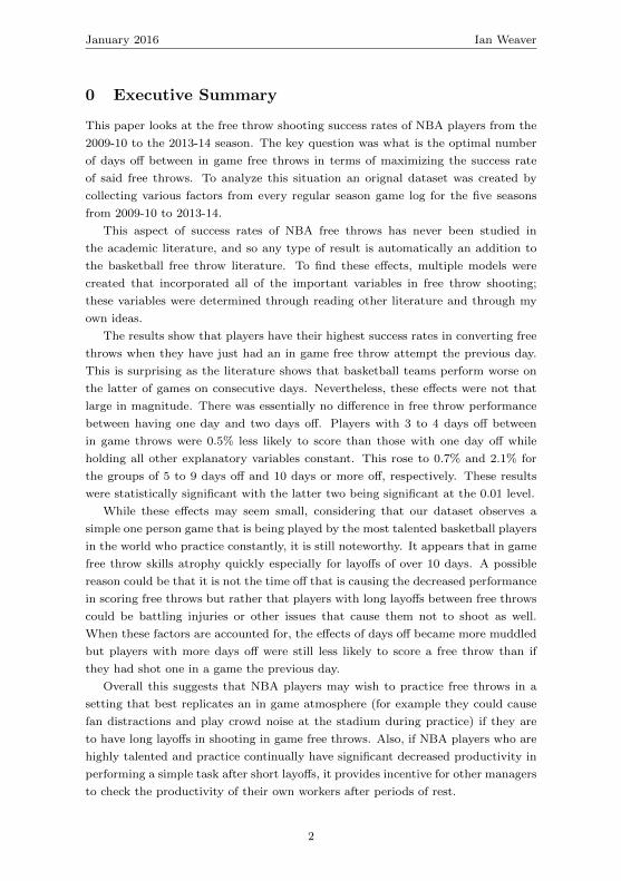
0 Executive Summary
This paper looks at the free throw shooting success rates of NBA players from the
2009-10 to the 2013-14 season. The key question was what is the optimal number
of days off between in game free throws in terms of maximizing the success rate
of said free throws. To analyze this situation an orignal dataset was created by
collecting various factors from every regular season game log for the five seasons
from 2009-10 to 2013-14.
This aspect of success rates of NBA free throws has never been studied in
the academic literature, and so any type of result is automatically an addition to
the basketball free throw literature. To find these effects, multiple models were
created that incorporated all of the important variables in free throw shooting;
these variables were determined through reading other literature and through my
own ideas.
The results show that players have their highest success rates in converting free
throws when they have just had an in game free throw attempt the previous day.
This is surprising as the literature shows that basketball teams perform worse on
the latter of games on consecutive days. Nevertheless, these effects were not that
large in magnitude. There was essentially no difference in free throw performance
between having one day and two days off. Players with 3 to 4 days off between
in game throws were 0.5% less likely to score than those with one day off while
holding all other explanatory variables constant. This rose to 0.7% and 2.1% for
the groups of 5 to 9 days off and 10 days or more off, respectively. These results
were statistically significant with the latter two being significant at the 0.01 level.
While these effects may seem small, considering that our dataset observes a
simple one person game that is being played by the most talented basketball players
in the world who practice constantly, it is still noteworthy. It appears that in game
free throw skills atrophy quickly especially for layoffs of over 10 days. A possible
reason could be that it is not the time off that is causing the decreased performance
in scoring free throws but rather that players with long layoffs between free throws
could be battling injuries or other issues that cause them not to shoot as well.
When these factors are accounted for, the effects of days off became more muddled
but players with more days off were still less likely to score a free throw than if
they had shot one in a game the previous day.
Overall this suggests that NBA players may wish to practice free throws in a
setting that best replicates an in game atmosphere (for example they could cause
fan distractions and play crowd noise at the stadium during practice) if they are
to have long layoffs in shooting in game free throws. Also, if NBA players who are
highly talented and practice continually have significant decreased productivity in
performing a simple task after short layoffs, it provides incentive for other managers
to check the productivity of their own workers after periods of rest.
2

January 2016 Ian Weaver
1 Introduction
1.1 Motivation
A common thought is that rest is a good for the performance of an individual. This
is difficult to refute as one would likely not suggest staying up all night the day
before an exam. Likewise, however, one would not likely suggest to take a few days
off to rest and not study before an exam. This causes a grey area on what type of
rest is best for an individual when they are trying to maximize their productivity.
An interesting question is whether managers get higher performance out of
their employees on Monday after they have gotten time off from work (but have
had their skills atrophy) or on Friday when they are tired of work (but their skills
are sharp from continual practice). Unfortunately, this is a difficult and nuanced
problem to answer. One area that does have a plethora of well documented data
to take a stab at this problem is the world of professional sports. However, sports
are played as one team directly against another which means that the success of
one team is directly related to the success of other team; this means that even if
one performs badly as long as the other team is worse then it is a positive result.
This is not particularly representative of the problem that managers face in getting
the most out of their employees. While their employees may have opponents it
is more likely that their task could be modeled as a one person game under the
exogenous restrictions placed on them by the world. Fortunately, there is one part
of basketball known as the free throw which is a one person game. For this reason,
this paper makes a small step forward in answering how time off between work
affects performance by looking at how well professional basketball players perform
under varying circumstances.
1.2 Outline
More specifically, the question this paper investigates is how does the number of
days between games effect the performance of NBA players in scoring a free throw
shot.1. The free throw is a simple one person game as it has no opposition. It also
something that NBA players will have practiced their entire life on their way to an
NBA career. Considering these are the most skilled players in the world performing
a simple task that they practice regularly, it would not be surprising if an extra
day off between games had no effect on their performance; yet this is not the case.
The way this will be investigated is by creating a binary outcome model where
the result of the free throw is the binary independent variable. Next multiple
specific models will be created by using a plethora of control variables and by
altering the variables that consider the time off between games. The probit model
1A free throw in basketball is an unimpeded shot at the net from a set line 15 feet away andoccurs due to infractions committed by the other team
3
January 2016 Ian Weaver
will be used as it accommodates any pattern of correlation and heteroskedasticity
in the error term.
The result of this paper will be useful in two ways. First, it will be useful to those
interested in sports analytics as it will give a direct result on how the schedule of
the NBA season affects the abilities of an NBA player to score a free throw. Second,
it will provide an interesting case study in how employee performance is affected
due to time off between work even when the task is fairly simple, the employee has
large amounts of practice in the task and the employee is skilled at the task.
2 Literature Review
There is a small section of literature dedicated to the effects of travel and days rest
on the ability of basketball players to perform; a subsection of this is even focused
on the ability to shoot free throws. A technique used in the life sciences is to create
an experiment such as Mah et al. [1] where they considered the effects of sleep
extension on the performance of collegiate basketball players. They discovered
that when the average sleep per night was increased by 2 hours that free throw
shooting percentage increased by 9%. Such a technique is not really applicable
here as these shots are taken in non game situations, and it measures sleep per
night rather than days between free throws (though there may be a correlation
between these).
A more relevant area of literature are econometric approaches which attempt to
ascertain the ability of basketball players to perform given varying schedules dic-
tated to them by the NBA. To the author’s knowledge, there exists no econometric
paper in the literature that examines these effects on the rate of success of players’
in scoring free throws. There are, however, a couple papers that consider the effect
of the NBA schedule on the ability of teams to win [2,3]. Due to the similarity, the
models in these papers will be pertinent in shaping our own models.
In both of these papers regressions are run by using point differential between
the home and away team as the dependent variable; common independent variables
include the strengths of both teams, whether they were home or away team and the
number of days of rest teams had before the game. The Steenland and Deddens
(SD) article also includes independent variables for travel such as distance, time
zones and directions travelled between games [2]. Overall both articles came to the
conclusion that teams did significantly worse when there was no off day between
games as compared to games where they had at least one day off between games.
Further, SD concluded that it was optimal to have two full days of rest between
games. Additional conclusions were that days rest affected the home and away team
equally (ES), and that duration and direction of travel did not have a significant
effect except when travelling from one coast to the other (SD).
4
January 2016 Ian Weaver
ES also repeated the analysis using a binary dependent variable on whether the
team won or not; this method, though, did not lead to any significant results. Part
of the reason for this may be an econometric criticism that I have with that model.
Their proxy variable for team ability was just that season’s team winning percentage
which by itself has a direct linear relationship with the dependent variable. As
a result the effects of rest and home court advantage that they were trying to
determine were partially being included in their variable for ability. For example,
consider a team with a tough schedule in terms of rest days (perhaps they have
more back to back games and then long layoffs than other teams). Their winning
percentage (and thus proxy for ability) will be lower than their actual ability to
win as the effects of the tough schedule are already erroneously being included in
their proxy variable. As a result, when they determined the effects of rest, it was
diminished as it is already being included to a certain degree into the proxy variable
for ability. This is likely why their model resulted in no conclusive results. This is
also something that must be taken into account in determining the proxy variable
for ability in free throw shooting in our own models.
The one econometric/statistical paper that could be found on free throw shoot-
ing was a project on how crowd behaviour affected players’ ability to score free
throws [4]. They showed through some statistical models that the home team was
less likely to score a free throw in a “high pressure” situation in comparison to
the away team. Their reasoning was that fans cheer loudly to try and distract the
away team player when he is shooting and are silent when the home team player is
shooting; however, a stadium full of silent fans creates an environment that makes
it more difficult to score free throws then when everyone is cheering. Regardless,
“high pressure” situations occur almost solely during close games in the final quar-
ter. As a result this research suggests two new control variables for our regressions:
the quarter in which the shot occurs and the score differential at the time of the
shot.
3 Data
3.1 Data Source and Variables
The data for this project comes from NBA game logs that are available at Basket-
ball Reference [5]. Using these game logs, I wrote programs which stripped relevant
information about every free throw that was taken in the regular season in the NBA
between the 2009-2010 season and the 2013-2014 season. These relevant variables
include whether the shot was scored, the ability of the player shooting, the date the
shot was taken, the quarter the shot was taken, the score differential of the game
when the shot was taken, whether the player was home or away when taking the
shot, the days rest the player had before taking the shot, whether the player took
5
January 2016 Ian Weaver
a free throw last game, and the number of time zones the player travelled before
taking the shot. Most of these were inspired by the papers from the literature
section except for a few that I added myself. Variables like height, age, etc. were
not included even though they have an effect on scoring free throws as they are
all encompassed in the variable of ability. The variables are specifically described
below.
score - A binary variable that is 1 if the free throw is scored and 0 if the free throw
is missed
ftability - A measure of the ability of the free throw shooter (will be formulated
in Section 4).
home - A binary variable that is 0 if the game was played away and 1 if the game
was played at home
date - A binary variable that is 0 if the free throw was taken in the first half of the
season and 1 if it was taken in the latter half of the season
quarter - The quarter that the free throw was taken. 1 stands for first quarter, 2
for second quarter etc.
daysrest - The number of days between the game in which the current free throw
was shot and the last game in which he attempted a free throw
playedprev - A binary variable that is 1 if the free throw shooter had a free throw
attempt in the last game that his team played and 0 otherwise
absscorediff - The absolute score difference in the game at the time of the shot
timediff - The difference in time between the time zone that the current free throw
is being taken and the time zone that the team last played in (travelling east to
west is negative and travelling west to east positive)
abstimediff - The absolute value of timediff
As some of these definitions are nuanced, here is an example to illustrate what
is meant. Assume that a team plays on January 1st, 2nd and 4th. A certain player
attempts and scores exactly one free throw on both January 1st and January 4th;
he attempts none on January 2nd. Also, the games on January 1st and 4th are
6
January 2016 Ian Weaver
played in the Eastern Time Zone while the one on January 2nd is played in the
Central Time Zone. So for the shot on January 4th, daysrest = 3 as the last game
he attempted a free throw was January 1st. playedprev is 0 as he did not attempt
a free throw in the last game his team played. timediff is 1 as he is currently in
a time zone that is one hour ahead of the time zone that his team last played.
Here we have chosen daysrest to be the time between in game free throw at-
tempts and not the time between games played in. This is because here we are
interested in measuring the effect on performance of total time off from doing a
task in a work setting as opposed to the effect on performance of total time off
from work. Also we have denoted daysrest to be 5 for free throws shot in season
openers as on average there is 5 days between when a team last plays a pre-season
game and the start of their regular season.
The variable playedprev is of potential interest because it could be that those
players who often do not have a free throw attempt in a game are having their
ability to score affected by things other than the time between in game free throws.
For example they may be battling injuries and this may be affecting their usual free
throw performance in ways we can not observe. If we do not include playedprev
then we will be incorporating some of the effects of the injury into daysrest.
The variable timediff measures the time zone difference between the time zone
of the game in which he currently shot a free throw and the time zone of the game
that his team last played in. This is because it is assumed that the player travels
with the team even when he gets limited playing time, is benched or is injured
(sometimes for larger injuries they do not travel with the team, but there is no way
of tracking their movements so it will be assumed that they at least start travelling
with the team just before their return).
Further, daylight savings was included when applicable in the calculations of
timediff . Interestingly, the state of Arizona does not observe daylight savings
time while every other state with an NBA franchise does. This is only a minor
point for this paper, but may be of use to others who are trying to separate the
effects of distance travelled and time zones travelled.
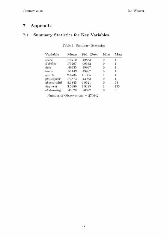
3.2 Summary of Key Statistics
A summary of the key statistics is given in Table 7.1 in the appendix. The main
results were that over the 5 seasons from 2009-10 to 2013-14 there were 276642 free
throws taken and 75.7% of these were scored. Other interesting results are that
51.1% of free throws were for the home team (which suggests either referee bias or
that teams play better at home), more free throws occur in the second half of a
game than the first half (as mean of quarter = 2.67 > 2.5) and that 73.9% of free
throws are taken by players who attempted at least one free throw in the previous
game that their team played in.
7
January 2016 Ian Weaver
4 The Econometric Model
4.1 The Basic Model
To achieve the basic econometric model, all of the free throws from the 2009-10
to 2013-14 season were pooled together into one cross section. This can be done
as time should not be affecting any variables except for ability and we allow this
variable to change every season. Once the other factors in our model have been
accounted, then will use a probit model.
The basic econometric model is described by the following equation:
score = β0 + β1ability + β2daysrest+ control variables+ µ
In this equation the dependent variable is score which is a binary variable that is 1
if the free throw was scored and 0 if it was missed. The main variable is daysrest
as the goal of the paper is to see how the amount of time off between free throws
affects a player’s ability to shoot a free throw. There are also numerous control
variables as listed in section 3.1. Different uses of these variables and variations
of daysrest will provide all of the econometric regressions for this paper. Of the
control variables, ability is not actually observed, which is a problem that will be
dealt with shortly.
A main assumption in this model is that there is no correlation between the
unobservable error variables and the independent variables. This is a reasonable
assumption for two reasons. First there is no issue of simultaneity, as whether the
player scores his free throw is not affecting any of the explanatory variables. For
example, whether he scores or not does not explain which quarter he took the shot,
the score differential of the game, the amount of rest he had before the shot, his
ability to score free throws etc. Second, omitted variable bias will not be a problem
(with the exception of determining ability) as there is a wealth of data available on
any free throw attempt; any omitted variables would be our mistake in identifying
the model and not because we were unable to get data for a certain variable.
At this point, the regression for the basic model can run as soon as it is deter-
mined how to deal with ability which is not observed. Fortunately, a good proxy
variable exists and developing it will be the focus of the next section.
4.2 Finding a Proxy for Ability
4.2.1 Proposing a Proxy for Ability
A very natural proxy for ability would be to use the free throw percentages for
a particular season for the player of interest. Alternatively worded this is the
percentage of free throws that a particular player scored during a particular season.
8
January 2016 Ian Weaver
As an example, if the free throw was taken by Tim Duncan in 2011-12, then we
would use his free throw percentage from that year as a measure of his ability to
score that free throw. Intuitively, this should be a good estimator of the unobserved
ability of a player to score any given free throw.
Unfortunately there is one major problem with this estimator, which was alluded
to in Section 2. The issue is that a player’s free throw percentage for a given season
might not be completely representative of their actual unobserved ability. Each
season that player may have to take more 4th quarter free throws, more free throws
after long periods of not playing, more free throws in close games etc. as compared
to usual. However, we have hypothesized that these factors affect whether a player
will score a free throw, so by using the season free throw percentages as a proxy for
ability we are incorporating the exact effects we are trying to determine into our
proxy for ability.
To help ameliorate these issues, we will propose another proxy variable for play-
ers’ ability to score free throws. This variable is called ftability and it will be
the average free throw percentage of a player for all free throw attempts made by
that player during the season he took that free throw as well as the season before
and after that. This takes advantage of the fact that a player’s free throw ability
should change very little between consecutive seasons while giving more data so
that the estimates for ability will be less governed by randomness. Further, the
free throw percentage calculated over three seasons should be more accurate in
capturing a player’s true ability during the season that the free throw was taken
as it less prone to the particular characteristics of the free throws taken during the
season of interest.
This proxy does not solve all of the issues. Consider that a player may have
certain unobserved traits. For example, each season he may only play in lopsided
games. As a result he does not play often and this means he is placed in a dis-
proportionate amount of situations where he has a lot of time off between in game
free throws. Thus, he is regularly placed in tougher than normal situations to score
a free throw, which means that ftability will be lower than ability. Nevertheless,
these differences should be random among the entire sample and they should also
be very small now that the proxy includes three seasons instead of one.
The reason that we chose only 3 seasons instead of more seasons is because that
a player’s free throw ability can change over time. As evidence for this, consider
the case of Tim Duncan. Over the first 10 seasons of his career he had free throw
percentage of 67.75% while over the last 9 seasons he had a free throw percentage of
73.66%. By the t-test assuming unequal variances we reject the null hypothesis that
the two means are equal at the 5% significance level (p-value of 0.028). Whether
using three seasons is optimal is not known. Solving this problem would require
somehow balancing the issues with changing player ability over time, with the added
9
January 2016 Ian Weaver
benefit of gaining more seasons of data. Above we have intuitively argued for why
three seasons will make a very good estimator.
On a technical note when the player has no free throw information for the season
before or season after the season in which the free throw was taken then only the
data available is used. For example, if a player only played one year in the NBA,
then his ftability is just his free throw percentage for that one season.
4.2.2 Showing that ftability is a Good Proxy
According to Wooldridge [6], any good proxy variable should have certain prop-
erties. First, the assumption that µ is uncorrelated with ftability was already
discussed in section 4.1. The more controversial assumption needed is that
E(ability | explanatory variables) = E(ability | ftability)
This is the case if the average level of ability only changes with ftability and not
home, date, quarter, absscorediff , daysrest and timediff . This also seems a
reasonable assumption as why would a player’s natural ability to score free throws
be affected by variables determining where and when they were playing. Thus, our
proxy variable satisfies the assumptions to be a good proxy.
5 Empirical Results
5.1 Results of Basic Model by Probit Regression
By incorporating the proxy from section 4 into the basic model we get the following
equation, which we will estimate by probit:
score = β0 + β1ftability + β2home+ β3date+ β4absscorediff
+β5abstimediff + β6quarter + β7daysrest+ µ(1)
Note that this model has no interaction between dummy variables and other ex-
planatory variables, which means that it does not allow for a difference of slopes
for the different binary choices. For example, this means that it is assumed that
the return of an extra day off between free throw attempts is the same whether the
player was at home or away.
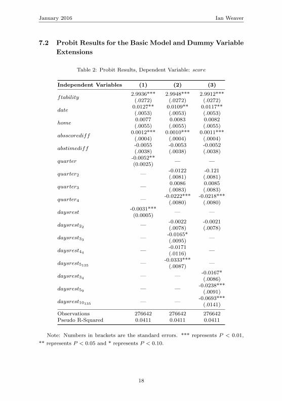
The results are found in Table 2, section 7.2 of the appendix. Using the hy-
pothesis test of H0 : Bi = 0 against H1 : Bi 6= 0 for any i ∈ {1, 2, 3, 4, 5, 6, 7},
almost all of our variables were significant at very small significance levels. The
other two variables (abstimediff and home had p-values under 0.15 which suggest
that they should not be dropped from the regression even if they provide results of
little interest on their own.
10
January 2016 Ian Weaver
The directions of the results are what was expected for almost of these variables.
Players score free throws with higher success rates when they have higher abilities,
when they play at home (home court advantage), when it is the latter half of the
season (more warmed up), when it is in the earlier quarters of a game (less tired),
when the score differential in the game is higher (less pressure), and when they
travel fewer timezones between games (less tired). The one exception is that of
rest between games. If the hypothesis that players do worse when they travel more
because travel is tiring is accepted then one would expect that more days between
free throw shots would improve scores. Nevertheless, it makes it more difficult with
a p-value less than 0.001. There could be a few reasons for this, which will be
explored shortly. For now, the takeaway is that the control variables are all very
reasonable.
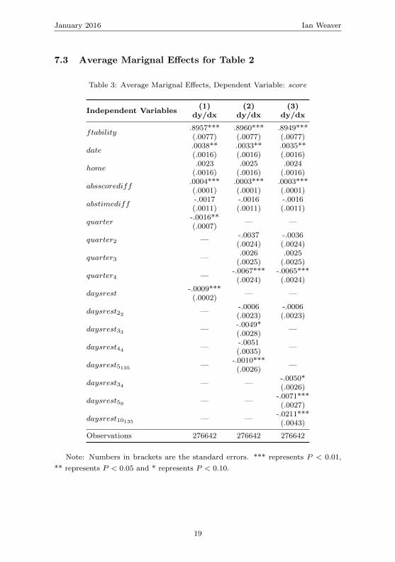
When the average marginal effects are calculated (Table 3 in the appendix) then
the results turn out not to be that drastic. With the exception of ftability all of the
independent variables have very small effects. For example, if the number of days
between games with a free throw is increased by 1 (while holding other independent
variables constant), then the average player is 0.09% less likely to score that free
throw. Despite being significant even at very low p-values, this is a very small effect
that will be of little interest to those with stakes in the game of basketball.
5.2 Probit Results using Dummy Variables for Rest
Part of the reason for the results in the previous section may be that the effects of
the number of days between free throws in games is not linear. To figure this out, a
method similar to Entine and Small (ES) [3] will be used, which is to partition the
daysrest variable into multiple dummy variables. With regards to notation, let us
denote daysrestij as a dummy variable that is 1 if the player had between i and
j days (including boundaries) between the game in which the current free throw
was shot and the last game in which the same player attempted a free throw; it is
0 otherwise.
At this time the basic model will also be altered to consider the effects of each
quarter separately by creating dummy variables. That is quarterk is a dummy
variable that is 1 if the shot was taken in the kth quarter and 0 otherwise.
Two regressions will be run. The first will partition the set of number of
days between in game free throws as {{1}, {2}, {3}, {4}, {5, ...135}} while the sec-
ond will partition the set of number of days between in game free throws as
{{1}, {2}, {3, 4}, {5, 6, 7, 8, 9}, {10, ..., 135}}. This covers the entire data set as daysrest
has a value between 1 and 135 for every observation in our data set. In terms of
equations these are written as follows with the first partition being represented
in equation (2) and the second partition in equation (3). Here our base group is
daysrest11 , so it is not included in the regression equation.
11
January 2016 Ian Weaver
score = β0 + β1ftability + β2home+ β3date+ β4absscorediff+
β5abstimediff +
4∑k=2
αkquarterk +
4∑i=2
γidaysrestii + γ5daysrest5135 + µ(2)
score = β0 + β1ftability + β2home+ β3date+ β4absscorediff+
β5abstimediff +
4∑k=2
αkquarterk + γ2daysrest22 + γ3daysrest34+
γ4daysrest59 + γ5daysrest10135 + µ
(3)
The only difference between our model in equation (1) and those in (2) and (3)
is how quarter and daysrest are partitioned in dummy variables. In both models
(2) and (3), both quarter2 and quarter4 are negative. This means that players
are less likely to score a free throw during the 2nd or 4th quarter than in the 1st
quarter (holding all of the other independent variables constant). As quarter3 is
not statistically significant then overall the negative coefficients of quarter2 and
quarter4 may be because players get tired throughout the game. However, this is
likely not the whole situation as quarter4 is much more significant then quarter2
and has a much larger average marginal effect. Indeed in model (2) the average
player is 0.67 percentage points (0.65 percentage points in model (3)) less likely to
score a free throw in the fourth quarter as compared to the first quarter. While this
is still a small effect, considering how consistent NBA players are this is noteworthy.
The main question is what are the effects of the dummy variables for daysrest.
In the model from equation (2), it is obtained that there is no significant difference
between two days between in game free throws and one day. For the groups of
three days and four days, these both have small negative effects with p-values
around 0.10. In fact, when a regression was run that gave every amount of days
off between in game free throws a separate dummy variable, similar effects and p-
values were obtained for each variable. Part of the problem is a lack of observations
for many of these dummy variables, which is why different grouping is necessary.
Using the results of model (2) as motivation, we obtain the groupings for equa-
tion (3). The difference here is that days off of three and four days have been
grouped into one dummy. Further instead of having 5 or more days off as a one
dummy this has been separated into two dummy variables (5 to 9 days and 10 days
or more). The results were that the average player is 0.5 percentage points less
likely to score a free throw with three or four days between in game free throws
as compared to having one day off between in game free throws (while holding all
other independent variables constant). For the groups of 5 to 9 days and 10 days
12
January 2016 Ian Weaver
or more, the average marginal effects were 0.7% and 2.1% respectively. The latter
of these has a p-value less than 0.001 and 2.1% is actually a fairly large effect.
Nevertheless, it may be expected that after such a large layoff that a decrease in
productivity would be expected.
Perhaps the more interesting result is that even for periods of time of three or
four days (which are fairly normal time periods between games), that players were
0.5 percentage points less likely to score a free throw than if it had only been one
day off. The results in the academic literature [2,3,7] as well as conventional wisdom
suggest that teams play worse on the second of consecutive games as compared to
a larger (though standard) amount of days between games. However, free throws
provide an example where players perform significantly worse and by an appreciable
amount (considering how consistent NBA players are in performing this simple
task).
5.3 How Does Being In and Out of the Lineup Affect Free
Throw Shooting
Possibly the biggest concern to the previous models is that it treats all layoffs
between in game free throws as the same even this may not be the case. For
example, a player coming back from an injury may shoot worse than if he had
not been coming back from an injury (holding days between free throws constant).
Another example is that a coach observes that his player is not playing well and so
he gets less playing time and often goes games without a free throw. He may shoot
worse during these periods than periods where he is playing well and regularly
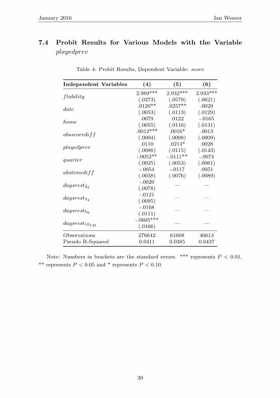
scoring free throws. Whatever the case, to account for this the variable playedprev
will be added to the model given by equation (3). It is a binary variable that is 1 if
the free throw shooter had a free throw attempt in the last game his team played
and 0 otherwise. The updated model is represented by the following equation:
score = β0 + β1ftability + β2home+ β3date+ β4absscorediff+
β5abstimediff + β6playedprev + β7quarter + γ2daysrest22+
γ3daysrest34 + γ4daysrest59 + γ5daysrest10135 + µ
(4)
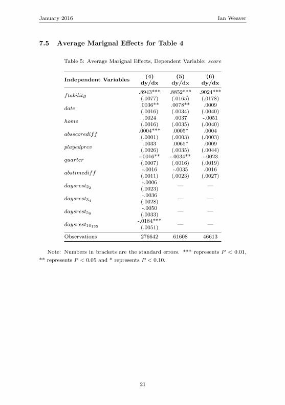
As predicted, playedprev is positive which means that a player that had a free
throw attempt in his team’s last game is more likely to score his free throw than if
he did not have a free throw attempt in his team’s last game (while holding days
off and other independent variables constant). The introduction of playedprev also
decreased the average marginal effects of our dummy variables for daysrest by
about 30%.
Unfortunately, playedprev is not statistically significant and the p-values for
the days off dummy variables have grown greatly rendering many of those results
13
January 2016 Ian Weaver
not statistically significant. This is not that surprising as there is a strong correla-
tion between playedprev and the daysrest. Indeed due to NBA scheduling, when
dayrest is less than or equal to 2 then playedprev must be equal to 1. If daysrest
is greater than or equal to 10 then playedprev must be equal to 0.
To further investigate, two more regressions will be run on models which are
restricted to only observations with 3 or 4 days off between in game free throws or
only observations with 5 to 9 days off separately. In terms of model specification,
both (5) and (6) follow the restricted model represented by the equation below.
The difference is that (5) is restricted to those observations where daysrest34 = 1
and (6) is restricted to those observations where daysrest59 = 1.
score = β0 + β1ftability + β2home+ β3date+ β4absscorediff+
β5abstimediff + β6playedprev + β7quarter + µ
When the data set is restricted to observations where daysrest34 = 1 , playedprev
was statistically significant with a p-value of 0.053. Further, the average player is
0.65% more likely to score a free throw if he had a free throw attempt in his team’s
last game than if he did not have a free throw attempt in his team’s last game
(holding all other independent variables constant). However, when the data set is
restricted to those observations with daysrest59 then playedprev is not statistically
significant (p-value of 0.845) and has an average marginal effect of 0.09%. In other
words, there is no discernible difference in free throw performance between those
who had an attempt in their team’s last game and those who did not.
Overall, the effects of playedprev are still unclear. I believe the problem could
be fixed with an even larger data set to overcome the collinearity issues.2 The
reason I believe this would work is because when the data set is restricted as it was
in (5) and (6), then date, absscorediff and quarter all had large changes in effects
as well as losing significance. The reason they all lost significance is likely due to
the lack of sample size; our trends are so subtle that even sample sizes of 50000 are
not enough. This is further supported by the fact that over the 5 season data set,
free throws are significantly harder to score in the 4th quarter than the 1st with
a very small p-value of 0.005. Yet when the calculations are restricted by season
there was one season where players actually performed better in the 4th quarter.
Thus, data sets of 50000 are not large enough to accurately the effects that we are
interested in.
2This is unfortunately something that I did not have time to do under the time constraintsof this course.
14
January 2016 Ian Weaver
6 Conclusion
This paper looks at the effects of time off between games on the free throw shooting
of professional basketball players. It concludes that players are their best at free
throw shooting when they had an in game free throw attempt the previous day.
This is an interesting result as the current literature and wisdom supports the
notion that players perform worse when they have to play two days in a row and
yet this is one aspect of the game where they perform better.
For the most part, the advantages to having attempted an in game free throw
the previous day are quite small and thus not of much use to those with a stake
in basketball games. For layoffs of over 10 days, though, these effects are over 2%,
which suggest that NBA players with long layoffs may wish to practice free throws
in a setting that best replicates the game atmosphere before they return .
Ignoring the effects on the game of basketball itself, it is a noteworthy result
in that even small amounts of time off from performing this task during a game
can lead to decreased productivity. Considering this is a simple one player task
that is being completed by the most talented players in the world who practice
the task continually in non-game scenarios under the best coaches, it is slightly
surprising that even a few days off between in game performance of the task could
lead to a significant decrease in the ability to perform it. This provides incentive
for other managers to check the productivity of their own workers after periods of
time off as a further research project. They likely have employees with less training
and less dedication, performing tasks that are more complicated than the situation
described in this paper, and so their decrease in productivity may be even larger.
15

January 2016 Ian Weaver
References
[1] Mah, Cheri D. et al. ’The Effects Of Sleep Extension On The Athletic Perfor-
mance Of Collegiate Basketball Players’. SLEEP (2011): n. pag. Web.
[2] Steenland, Kyle, and James Deddens. ’Effect Of Travel And Rest On Perfor-
mance Of Professional Basketball Players’. Sleep 20.5 (1997): 366-369. Print.
[3] Entine, Oliver A, and Dylan S Small. ’The Role Of Rest In The NBA Home-
Court Advantage’. Journal of Quantitative Analysis in Sports 4.2 (2008): n. pag.
Web.
[4] Goldman, Matt and Justin Rao. ’Effort vs. Concentration: The Asymmetric
Impact of Pressure on NBA Performance’. MIT Sloan Sports Analytics Conference
(2012): n. pag. Web.
[5] Basketball-Reference.com,. ’Basketball-Reference.Com’. N.p., 2015. Web. 8
Dec. 2015.
[6] Wooldridge, Jeffrey M. Introductory Econometrics. Australia: South-Western
College Pub., 2003. Print.
[7] Sampaio, Jaime, Eric J. Drinkwater, and Nuno M. Leite. ’Effects Of Season
Period, Team Quality, And Playing Time On Basketball Players’ Game-Related
Statistics’. European Journal of Sport Science 10.2 (2010): 141-149. Web.
16
January 2016 Ian Weaver
7 Appendix
7.1 Summary Statistics for Key Variables
Table 1: Summary Statistics
Variable Mean Std. Dev. Min Max
score .75710 .42883 0 1ftability .75797 .09532 0 1date .49435 .49997 0 1home .51143 .49987 0 1quarter 2.6735 1.1035 1 4playedprev .73873 .43933 0 1absscorediff 8.1845 6.9521 0 54daysrest 3.5380 4.9129 1 135abstimediff .45028 .70622 0 3
Number of Observations = 276642
17
January 2016 Ian Weaver
7.2 Probit Results for the Basic Model and Dummy Variable
Extensions
Table 2: Probit Results, Dependent Variable: score
Independent Variables (1) (2) (3)
ftability2.9936***
(.0272)2.9948***
(.0272)2.9912***
(.0272)
date0.0127**(.0053)
0.0109**(.0053)
0.0117**(.0053)
home0.0077(.0055)
0.0083(.0055)
0.0082(.0055)
absscorediff0.0012***
(.0004)0.0010***
(.0004)0.0011***
(.0004)
abstimediff-0.0055(.0038)
-0.0053(.0038)
-0.0052(.0038)
quarter-0.0052**(0.0025)
— —
quarter2 —-0.0122(.0081)
-0.121(.0081)
quarter3 —0.0086(.0083)
0.0085(.0083)
quarter4 —-0.0222***
(.0080)-0.0218***
(.0080)
daysrest-0.0031***(0.0005)
— —
daysrest22 —-0.0022(.0078)
-0.0021(.0078)
daysrest33 —-0.0165*(.0095)
—
daysrest44 —-0.0171(.0116)
—
daysrest5135 —-0.0333***
(.0087)—
daysrest34 — —-0.0167*(.0086)
daysrest59 — —-0.0238***
(.0091)
daysrest10135 — —-0.0693***
(.0141)
Observations 276642 276642 276642Pseudo R-Squared 0.0411 0.0411 0.0411
Note: Numbers in brackets are the standard errors. *** represents P < 0.01,
** represents P < 0.05 and * represents P < 0.10.
18
January 2016 Ian Weaver
7.3 Average Marignal Effects for Table 2
Table 3: Average Marignal Effects, Dependent Variable: score
Independent Variables(1)
dy/dx(2)
dy/dx(3)
dy/dx
ftability.8957***(.0077)
.8960***(.0077)
.8949***(.0077)
date.0038**(.0016)
.0033**(.0016)
.0035**(.0016)
home.0023
(.0016).0025
(.0016).0024
(.0016)
absscorediff.0004***(.0001)
.0003***(.0001)
.0003***(.0001)
abstimediff-.0017(.0011)
-.0016(.0011)
-.0016(.0011)
quarter-.0016**(.0007)
— —
quarter2 —-.0037(.0024)
-.0036(.0024)
quarter3 —.0026
(.0025).0025
(.0025)
quarter4 —-.0067***(.0024)
-.0065***(.0024)
daysrest-.0009***(.0002)
— —
daysrest22 —-.0006(.0023)
-.0006(.0023)
daysrest33 —-.0049*(.0028)
—
daysrest44 —-.0051(.0035)
—
daysrest5135 —-.0010***(.0026)
—
daysrest34 — —-.0050*(.0026)
daysrest59 — —-.0071***(.0027)
daysrest10135 — —-.0211***(.0043)
Observations 276642 276642 276642
Note: Numbers in brackets are the standard errors. *** represents P < 0.01,
** represents P < 0.05 and * represents P < 0.10.
19
January 2016 Ian Weaver
7.4 Probit Results for Various Models with the Variable
playedprev
Table 4: Probit Results, Dependent Variable: score
Independent Variables (4) (5) (6)
ftability2.989***(.0273)
2.932***(.0579)
2.933***(.0621)
date.0120**(.0053)
.0257**(.0113)
.0029(.0129)
home.0079
(.0055).0122
(.0116)-.0165(.0131)
absscorediff.0012***(.0004)
.0016*(.0008)
.0013(.0009)
playedprev.0110
(.0088).0214*(.0115)
.0028(.0143)
quarter-.0052**(.0025)
-.0111**(.0053)
-.0074(.0061)
abstimediff-.0054(.0038)
-.0117(.0076)
.0051(.0089)
daysrest22-.0020(.0078)
— —
daysrest34-.0121(.0095)
— —
daysrest59-.0168(.0111)
— —
daysrest10135-.0605***(.0166)
— —
Observations 276642 61608 46613Pseudo R-Squared 0.0411 0.0385 0.0437
Note: Numbers in brackets are the standard errors. *** represents P < 0.01,
** represents P < 0.05 and * represents P < 0.10.
20
January 2016 Ian Weaver
7.5 Average Marignal Effects for Table 4
Table 5: Average Marignal Effects, Dependent Variable: score
Independent Variables(4)
dy/dx(5)
dy/dx(6)
dy/dx
ftability.8943***(.0077)
.8852***(.0165)
.9024***(.0178)
date.0036**(.0016)
.0078**(.0034)
.0009(.0040)
home.0024
(.0016).0037
(.0035)-.0051(.0040)
absscorediff.0004***(.0001)
.0005*(.0003)
.0004(.0003)
playedprev.0033
(.0026).0065*(.0035)
.0009(.0044)
quarter-.0016**(.0007)
-.0034**(.0016)
-.0023(.0019)
abstimediff-.0016(.0011)
-.0035(.0023)
.0016(.0027)
daysrest22-.0006(.0023)
— —
daysrest34-.0036(.0028)
— —
daysrest59-.0050(.0033)
— —
daysrest10135-.0184***(.0051)
— —
Observations 276642 61608 46613
Note: Numbers in brackets are the standard errors. *** represents P < 0.01,
** represents P < 0.05 and * represents P < 0.10.
21