Embrace or Eschew? Position Taking on Unpopular Presidents in Senate Elections

Neilan S. ChaturvediAssistant Professor

California Polytechnic University, Pomona

Chris HaynesAssistant Professor

University of New Haven

Prepared for presentation at the Annual Meeting of the Western Political Science Association, San Diego, CA 2016

AbstractWhen faced with an unpopular president, incumbents have the difficult task of deciding whether to eschew the president, embrace him, or find some middle ground of ambiguity. Indeed, political science scholarship finds there are electoral incentives to silence and ambiguity on the campaign trail on salient issues, yet there is little evidence of an optimal strategy when running for reelection with an unpopular president. In this paper, we test the optimal reelection strategy for senators running for reelection when their party’s president is unpopular. Using data from a survey experiment conducted using a national sample, we examine the responses towards three hypothetical Democrats: (i) supportive of Obama (ii.) ambiguous about their attitude towards Obama (iii.) opposed to Obama. Comparing participants exposed to the ambiguous and the supportive Democrat, we find that the level of support and excitement for the candidate were essentially the same. We also find that participants exposed to the Democrat opposed to Obama were not more or less supportive of the Democrat, but were less excited and more negative towards that candidate. We also find that Democrats and Independents were increasingly negative and less excited the less the candidate supported Obama while Republicans were only marginally more excited and positive towards ambiguous or disloyal Democrats. Overall, these findings suggest that the optimal reelection strategy for Democratic candidates given an unpopular same-party president is to remain supportive.

1

Introduction

In 2008, voters ushered in large Democratic majorities in both the House and Senate along with a

newly elected Democratic President in Barack Obama. In the United States Senate, 35 of the 100

seats were contested and with an unpopular, though term-limited Republican president, voters

were eager for the change Obama and his fellow Democrats offered. Indeed, Democrats

expanded their majority in the Senate by winning eight seats. In a handful of those seats,

Democrats beat incumbent Republicans (i.e. Al Franken (D) defeating Norm Coleman (R) in

Minnesota and Jeff Merkley (D) defeating Gordon Smith (R) in Oregon). Additionally, the

Democratic tide was strong enough to elect Democrats in otherwise red Presidential states. For

example, Mark Begich (D) defeated long time incumbent Ted Stevens (R) in Alaska and little

known state senator Kay Hagan (D) defeated Elizabeth Dole (R) in North Carolina.

While much can be said about the effectiveness of campaign strategy and candidate

strength, ties to a popular Democratic presidential candidate and an unpopular outgoing

Republican president should not be dismissed. In North Carolina, Kay Hagan benefitted from

tying her opponent Elizabeth Dole (R) to Bush by running ads claiming that Dole voted with

Bush 92% of the time (Robertson 2014), though she also benefitted from the Obama turnout

machine in which Obama significantly increased turnout among blacks and young voters in

North Carolina (Miller and Chaturvedi 2009). Even Mark Warner, a Democrat running from the

swing State of Virginia spoke as the keynote speaker for Obama at the 2008 Democratic

National Convention, hoping to take advantage of some of the national momentum.

2

However, just two years into Obama’s presidency and as quickly as the Democrats were

swept into office, a counter-wave turned House control back over to the Republicans lost six

seats to the Republicans in the Senate. The debate and eventual partisan passage of Obamacare

alongside the slow economic recovery from the economic collapse of 2007 took its toll on

Obama’s approval rating. Most importantly, during both the 2010 and 2014 election cycles

(Labor Day through Election Day), not once was President Obama’s weekly approval rating

above water (net positive) (Gallup 2016). Thus, with Obama’s approval rating teetering in the

40s, Democrats in 2010 and 2014 were faced with a difficult decision—support an unpopular

president or create distance from him? For senators in liberal states, the decision was fairly easy,

remain supportive and blame the opposition. Indeed, in New Jersey, Cory Booker hosted a

fundraiser with Obama in 2014 (Johnson 2014). Yet those from swing states or from states

traditionally hostile to the Democratic Party had a much more difficult decision: should they

embrace their party’s embattled leader, ignore Obama altogether (ambiguous strategy), or

eschew him and draw a contrast? Clearly there was little agreement on the optimal strategy with

some Democrats like Mark Udall (D-CO) skipping an Obama fundraiser in his own state

(disloyal strategy) and others such as Kay Hagan (D-NC) physically embracing Obama at the

airport in Charlotte (loyal strategy). Indeed, data from the non-partisan Wesleyan Media Project

(WMP), which coded all political media ads used in the 2010 and 2012 elections shows that each

of these strategies were used by Democratic candidates in their U.S. Senate contests during both

election cycles. In particular, we find that five Democrats employed a disloyal strategy, one an

explicitly ambiguous strategy, ten an implicitly ambiguous strategy, and six a loyal strategy1.

1 The Wesleyan Media Project coded all political ads for each of the 2010 and 2012 U.S. Senate contests in terms of whether the ad explicitly mentioned President Obama and if so, if the ad explicitly stated that the candidate supported, opposed, or remained neutral to the President or his policy. We coded each Senate candidate in terms of their electoral strategy vis-à-vis President Obama. The coding strategy for each of the four electoral strategies was as follows: First, if a candidate ran any ads mentioning Obama, which ever type of ad (supportive, opposed, explicitly ambiguous) composed the plurality of the candidate’s ads determined their strategy label. For example,

3

That said, because so many other factors affect electoral outcomes (i.e. candidate quality,

challenger quality, electoral terrain), drawing any conclusions as to the effectiveness of each of

these strategies might be fraught with error.

So can we provide leverage on the question of what is the optimal strategy? Building on

scholarship employing experiments to examine the effectiveness of campaign strategy (Tomz

and Van Houweling 2008; 2009), we examine the optimal strategy for maximizing electoral

chances when running with an unpopular, same-party president. We examine three strategies and

their impact on voter opinions: embracing, eschewing, and offering an ambiguous position. We

find that candidates that embrace the president appeal to their base and independents, but lose

ground with the opposition. Alternatively, offering an ambiguous position or eschewing the

president depresses excitement and appeal among the base and independents. Most importantly,

this lost ground is not made up in the increase of support from the opposition.

This article proceeds as follows. We begin with a discussion about presidential coattails

and their diminishing value over the course of the president’s term. We then turn to the literature

on candidate positioning and messaging in campaigns. Following this section, we discuss our

data and our empirical results. We conclude with implications of our research and suggestions

for further areas of study.

Presidential Coattails

we coded Blanche Lincoln‘s (D-AR) strategy as “disloyal” as she ran 489 ads supporting Obama, 0 explicitly ambiguous ads (mention of Obama, but no indication whether candidate was supportive or opposed), 14,461 implicitly ambiguous ads (no mention of Obama) and 1501 ads opposing Obama. Alternatively, Richard Blumenthal (D-CT) ran 288 ads supporting Obama and 3701 implicitly ambiguous ads. Blumenthal’s strategy was coded as “supportive.” Second, if a candidate failed to run any ads mentioning or featuring Obama, they were assigned the code of “implicitly ambiguous.” For example, Paul Hodes (D-NH) was assigned the code of “implicitly ambiguous” since he only ran 2426 ads, none of which mentioned President Obama.

4

In their study on Senate elections and presidential coattails, James Campbell and Joe Sumners

(1990) aptly assess, “Only presidential elections are better finance are more competitive, involve

more experiences and well known candidates, and receive more media and public attention than

U.S. Senate elections.” Indeed, when compared to Congress’ other chamber, Senate incumbents

and their challengers are generally more recognizable to the electorate and spend much more

money as well (Jacobson 2006). Still, despite being fairly prominent figures on the American

electoral stage, voters still use cues to make voting decisions on Senate elections.

One factor that serves as a prominent cue for voters is the president’s performance. As

numerous studies demonstrate, voters exercise their disapproval of the president’s performance

by voting their co-partisans out of office, especially during midterm elections (Abromowitz

1984; 1985; Abramowitz and Segal 1992; Campbell and Sumners 1990; Cover 1986; Jacobson

1997; Kernell 1977; Marra and Ostrom 1989; Tufte 1975). As mentioned above, evidence from

the 2010 and 2014 elections show that this trend has not diminished in recent history.

In their seminal work on retrospective voting in congressional elections, Hibbing and

Aford (1981) argue that short-term economic performance of the national economy impacts the

Congressional incumbents from the president’s party using analysis from a 1978 survey. They

conclude, “Voters do not simply blame the president’s entire party; rather they seem to assign

blame selective, based on objective responsibility” (Hibbing and Aford 1981, 437). That is to

say, voters assign blame and credit to the “in party” Senators, or those incumbent Senators from

the president’s party. Fiorina (1983) goes on to offer more evidence to this argument using a

different methodology and five more election studies.

Still, others argue that this is only party of the electoral equation determining vote choice

in Senate elections. Fenno’s (1978) book entitled, Homestyle documents how members of

5

Congress create their own brand at home by claiming credit for policies they supported while

distancing themselves from others. This is of course, a key strategy for many members of the

United States Senate. In 2014 for example, Senator Jack Reed, an incumbent from Rhode Island

voted with his party almost 99 percent of the time. Meanwhile, more vulnerable senators like

Mark Pryor and Mary Landrieu voted with their party leadership 89 and 92 percent of the time,

respectively (source: voteview.com). This is, of course, not without reason. Senators from states

that are naturally hostile to the president have more reason to distinguish themselves from the

party and the president. Political science scholarship demonstrates that senators that vote with the

unpopular president are ultimately punished for their loyalty by their constituents, when

compared to their less loyal counterparts (Brady et al. 1996; Brady et al. 2000). Indeed, there is

evidence to suggest that these moderate senators that are perpetually in electoral danger shy

away from giving their opposition fuel by avoiding the political limelight (Chaturvedi 2016).

Gronke et al. (2003) claim that savvy members of Congress alter their voting patterns to

shift their constituent’s views on how supportive they are towards the president and his agenda

which in turn affects how constituents decide to vote for them. Using survey data from the

American National Election Studies from 1993, 1994, and 1996, Gronke et al. find that voters

are capable of accurately measuring their representative’s support for the president, and that they

use this as an effective heuristic for their vote choice. That is to say, voters assess the president

and in turn their representative’s support for the president, using this to determine their vote

choice.

This is where we seek to make our contribution to the literature. As the literature has

demonstrated, presidents do have an effect on the vote share of their co-partisans. Particularly

savvy members of Congress will then seek to manipulate this effect depending on the president’s

6

popularity: embrace the president when he is popular, eschew when he is unpopular. Yet over the

last several election cycles, senators from states that traditionally elect the opposing party or

from swing states have used this strategy to no avail. Indeed, senators like Jim Talent (R-MO),

Mike DeWine (R-OH) and Lincoln Chafee (R-RI) in 2006, and Mark Begich (D-AK), Mark

Pryor (D-AR), Mark Udall (D-CO), Mary Landrieu (D-LA), and Kay Hagan (D-NC) in 2014 all

made several efforts to distance themselves from Presidents Bush and Obama respectively.

Indeed, it is unclear what effect embracing the president has on the base compared to the

opposition’s voters. Furthermore, if the candidate eschews the president, what effect then does

this have on the base, and for that matter, is that enough for independents and the opposition to

then vote for the incumbent? As a result, we seek to answer when the eschew vs. embrace

strategy works and what effect it has on vote choice, excitement, and turnout.

Candidate Positioning

As mentioned in the previous section, senators running for reelection must be keenly aware that

the public will tie their vote with not only the incumbent’s performance, but also the president’s

performance. Savvy senators then, will need to establish a method in which to separate

themselves from their party’s president when that president is unpopular. In the previous section,

we discussed at length methods in which the senator may distance herself through her voting

record. Still, there is evidence to suggest that positioning and rhetoric may be another means to

separate the candidate from the president.

Indeed, in their experimental study examining the effects of tailored explanations for

particular votes and policy views, Grose et al. (2014) find that targeted explanations were

effective in influencing perceptions about the senator in question. Of course, this suggests that

7

such explanations give senators the ability to dismiss unpopular positions, thereby diminishing

their constituents’ ability to punish their representative. Though this may seem to be a cynical

view on representation and democracy, theorists have long argued that this sort of deliberation

with voters is a key to representation in that it forces the representative to engage her constituents

with regards to votes and decisions that are made on their behalf (Mansbridge 2003; Pitkin

1967). Still, it may be easier to offer targeted explanations for votes, but more difficult to offer

similar explanations for support or abandonment of a president.

Much of the work of explaining votes is in response to an opposition candidate.

Candidate positioning has often been studied under the framework of three major theories: the

proximity theory, or the idea that the candidate in the closest proximity to the majority of voters

wins the most votes (Downs 1957); the discounting theory, which argues that voters discount the

promises made by candidates and instead judge the candidates based on policies that are likeliest

to be implemented (Adams et al. 2004; Fiorina 1992; Grofman 1985); and the directional theory

which argues that the voters view issues as two-sided and that the candidate that is closest to

their side and the most intense about the issue are their candidates (Rabinowitz and MacDonald

1989). In their experimental study on how voters react to these strategies, Tomz and Van

Houweling (2008) find that proximity voting is two times more common as discounting and four

times as common as directional voting. This suggests that with regards to presidents, candidates

have an incentive to position themselves closest to their constituent’s approval or disapproval of

the president.

That would suggest that if the senator’s state approves of the president, the senator should

embrace the president and if the senator’s state disapproves of the president, the senator should

eschew the president. But what happens when the state does not have a clear opinion on the

8

president, like public opinion found in swing states. Perhaps even more exasperating for even the

savviest of senators, what is the senator to do when the base is supportive of the president but the

rest of the state isn’t? Another possible option would be to offer an ambiguous answer that limits

the senator’s ties to the president without offering specifics. This option is not without its

benefits. Shepsle (1972) argues that there may be a payoff for ambiguous candidates if the voters

are not risk averse. That is to say, voters who are risk averse may prefer the precise candidate,

but those that are willing to accept risk may buy into the ambiguity, but only if the ambiguity

comes from the challenger as the incumbent’s positions are typically well defined. Others have

found that voters may bias their opinion on ambiguous candidates by assuming that ambiguous

candidates side with them (Irwin 1953; Krosnick 2002; Rosenhan and Messick 1966). Tomz and

Van Howeling (2009) find that candidate ambiguity may have some positive effects on a

candidates vote share, especially in partisan elections.

Despite this, there is a distinction to be made between candidate positioning on the issues

and on an incumbent president. While there may be some payoff of ambiguity or even a

proximity based argument to cross sides on an issue, there may be less of a payoff for using these

strategies for the party’s president. While eschewing the president may help to appease angry

opposition voters, it cannot do much to excite the base of voters that are without doubt

supportive of the president. Indeed, even ambiguity has its faults as Campbell (1983) argues that

ambiguity could demonstrate an evasive or “spineless” persona. In the following sections, using

experimental data, we seek to provide answers as to the effectiveness of strategizing and position

taking on an incumbent president.

Data

9

To test these expectations examining how different Democratic candidate electoral

strategies running against a partisan Republican opponent might shift candidate support, we

conducted an original online Mechanical Turk survey experiment in the summer of 2015.2 The

sample included 1,049 different participants recruited via Amazon’s Mechanical Turk service

and referred to our Qualtrics-based survey-experiment. Participation was restricted to

individuals from U.S. IP addresses. Participants received an incentive of $.50 to take the 8-10

minute survey.

We focus on comparing the typical situation (Democratic candidate aligned with

President Obama) to that involving an ambiguous Democratic candidate OR to that involving a

Democratic candidate explicitly opposed to President Obama. More specifically and similar to

that used by Toms and Van Houweling (2008; 2009), participants were randomly assigned to

receive one of the following visual positioning prompts: typical Democratic candidate with

opposed Republican candidate (N=365), ambiguous Democratic candidate with opposed

Republican candidate (N=349), or disloyal Democratic candidate with opposed Republican

candidate (N=335). Figures 1-3 illustrate the images that were shown to the respective groups.

[Insert Figures 1-3 here]

All participants were then presented three questions used to measure candidate

preference, candidate affect, and candidate excitement. To gauge candidate preference,

participants were asked the following question (and multiple choice responses): “Which

candidate do you prefer?” (Democrat, Republican).

To measure candidate affect, participants were presented the following prompt asking

them to give a thermometer rating for each of the candidates: “Based on this information we

would like you to rate your feelings towards the candidates using a scale that we call a feeling

2 We use the unweighted data for these analyses since we can retain the full sample size.

10

thermometer. Ratings between 0-50 indicate that you don’t feel favorable toward the person and

that you don’t care too much for that person. Ratings between 50-100 indicate that you feel

warm towards that person and are favorable toward them. You would rate them at 50 if you don’t

feel particularly cool or warm towards them.  (Click on the vertical bar and pull it across the

scale to indicate your answer).” See Figure 4.

[Insert Figure 4 Here]

To measure candidate excitement, participants were presented the following prompt

asking them to give a thermometer rating for each of the candidates: “On a scale from one to ten,

where one means that you are not excited at all and ten means that you are very excited.  (Click

on the vertical bar and pull it across the scale to indicate your answer).” See Figure 5.

[Insert Figure 5 Here]

This was followed by two manipulation checks asking participants to separately identify

the positions vis-à-vis President Obama taken by each of the candidates. In short, our

manipulation was successful. The following are the percentages of participants that correctly

identified the position of the Democratic candidate: typical condition=92%, ambiguous

position=90%, disloyal condition=74%. Additionally, what follows are the same statistics for

correctly identifying the Republican candidate: typical condition=94%, ambiguous

position=93%, disloyal condition=94%.3

Finally, participants were asked to provide responses to a standard battery of socio-

political demographic questions. Sample composition was as follows: the average age was 36;

3 The results presented henceforth will be using data from participants that were able to correctly identify the position of the Democrat for their group. We ran our models twice, once with those that were not able to correctly identify the position correctly dropped, and another with them in the model. We found no difference in statistical significance and only a minimal change in the magnitude of the results. As a result, we choose to only present the results of the data with the dropped participants.

11

39% were male, 61% were female; the average education level was an associate’s degree and the

median respondent had a bachelor’s degree; the median respondent earned between $25,001 and

$50,000; the average respondent was midway between a weak liberal and a moderate; 50% said

they were liberal, 23% moderate, 27% conservative; 41% described themselves as Democrats,

20% Republicans, 30% independents; 82% were white, 10% black, 5% Latino, 6% Asian.

Additionally, the randomization process was largely successful given that only gender was not

distributed evenly across conditions. To this end, we ran two separate statistical models when

comparing mean differences between our three conditions (typical, ambiguous, disloyal) on each

of our three dependent variables (preference, affect, excitement), one model accounting for

gender as a balance check and another without. That said, results remain the same regardless of

model.

Results

Candidate Preference

Individuals were asked to select the candidate (Democrat or Republican) that they

supported given the information provided. We expect to see Democrats support the Democrat

regardless since the Democratic candidate will always be closer to their ideal position on

President Obama than an antagonistic Republican. Of more interest is how Republicans and

independents act towards the ambiguous and disloyal treatments. We first present the difference

in mean candidate preference for the Democratic candidate between each of the two conditions

as compared to the control group, respectively. These are presented in Figure 6.

[Insert Figure 6 Here]

12

Between the ambiguous treatment and the Control group, there is no significant difference in

candidate preference for any group. The figure displays large confidence intervals suggesting a

spurious relationship at best. This suggests that ambiguous position taking has no affect on

candidate preference. Indeed, participants, regardless of partisanship or ideology, showed no

significant change in their preference of the Democrat or Republican. On the surface, this

indicates a number of things. First, taking an ambiguous position on President Obama has no

effect on attracting independent, or Republican voters, nor moderate or conservative voters. In

short, ambiguity does not expand a senator’s coalition. Second, taking an ambiguous position on

President Obama also has no effect on Democratic or liberal voters. This lines up with what we

would expect to see. If voters are given a choice between a Democrat that partially supports the

President and a Republican that is antagonistic towards the president, Democratic voters should

still choose the Democrat.

Candidate preference did change when we examine the disloyal treatment in which the

Democratic candidate opposed President Obama. That said, the effects are small. The average

candidate preference shifted towards the Democrat for Independents by .16 and for

Republicans .08. However, once the imbalance between men and women in our sample was

taken into account, the difference in candidate preference for Republicans was no longer

significant. In terms of ideology, average candidate preference shifted towards the Democrat

by .04 for liberals and .14 for conservatives; however, neither difference retained its statistical

significance once the imbalance between men and women was taken into account. This runs

counter to conventional wisdom. If the strategy is to lure Republicans, Independents, moderates,

or conservatives, then the strategy clearly does not work, or does not work well enough to create

an advantage in terms of changing voters’ minds about who to vote for.

13

There was no significant shift for Democrats. Again, this is to be expected as a Democrat

would still support a candidate that has more overlap with their preferences than a Republican

that has very little overlap.

These results suggest that the ambiguity and the disloyalty strategy are both ineffective at

attracting support from voters that otherwise would not vote for them. Nevertheless, it is

premature to dismiss these strategies as ineffective as they may have a greater impact on

candidate affect and candidate excitement.

Candidate Affect

The second two graphs in Figure 6 present the difference in mean thermometer score between

the treatment groups and the control group. When participants were asked to rate their feelings

towards the Democrat, the mean difference between the ambiguous treatment and the control

group was again insignificant. This is somewhat more meaningful than the candidate preference

results and goes against our expectations. Indeed, an ambiguous position should increase the

feeling thermometer scores for independents, Republicans, moderates, and Conservatives.

However, the statistically insignificant differences suggest that ambiguity on the president offers

little to the Democratic candidate.

The disloyal treatment on the other hand does have some of the intended effects that we

would expect to see with Republican participants. For example, taking a position against the

president increases the thermometer scores for Republicans by 14.21 points, on average.

Additionally, for conservatives, the thermometer scores increase by 11.15 points, on average.

Still, Democratic participants did not respond as kindly to the slight against President Obama as

14

the difference between the control group score was -13.18 and for liberals it was -13.86, on

average. There was however, no significant difference for independents or moderates.

On the surface, this suggests that there may be some value in pursuing the strategy of

opposing Obama. However, this requires more context. Figure 7 displays the actual values of the

differences between the two groups.

[Insert Figure 7 here]

While the difference between the two groups of Republicans is large and significant, the points

gained for the Democrat are not nearly enough to create a positive or even indifferent opinion of

the candidate as the disloyal treatment group rated the Democrat at 38.77 on average. More

importantly, the candidate is doing quite a bit of damage with her base as she loses points and

moves closer towards indifference.

Candidate Excitement

Finally, we turn to how excited the participants were about voting for the Democratic candidate.

Figure 6 again shows the results of both the ambiguous treatment as well as the disloyalty

treatment. As with the previous results, there is no significant difference between the treatment

and the control group for the ambiguity experiment. This means that unlike position-taking on

the issues, ambiguity shows no overall change in feeling thermometer score or the respondent’s

excitement to vote for the candidate.

Again, we see significant differences between the disloyal treatment and the control

group. On average, the difference in excitement among Republicans was .99, on a scale running

from 1-10. Similarly, the difference among conservatives was .87, on average. This suggests that

Democratic candidates earn gains in enthusiasm among individuals that would not normally vote

15

for them. Yet, again, the difference between the disloyal treatment group Democrats and the

control group Democrats was negative in which the difference was -1.13. Again, similarly, the

score for liberals was -1.56, on average. Thus, while disloyal Democrats appear to post gains

among Republicans, they suffer even greater losses among co-partisans. To give greater context

to these numbers, Figure 8 shows the actual values between the two groups.

[Insert Figure 8 here]

Again, while the differences are significant, the excitement among Republican voters is not high

enough in the disloyal treatment to merit the strategy. Indeed, the excitement level remains well

below five, suggesting that while Republican voters are more positive and excited about voting

for the Democrat, there is little to suggest that they actually will vote for the Democrat.

Meanwhile, the loss in excitement among Democratic voters drops the excitement level to 5.4.

Even worse for the Democratic candidate, excitement to vote for the candidate amongst liberals

falls to below 5.0 at 4.77, on average. This suggests that the strategy, while successful in

changing opinions in favor of the Democrat for Republican and conservative participants, does

not efficiently add support and actually may do more harm than damage. We discuss the

implications and conclusions of these results in the following section.

Conclusions and Implications

Determining what helps and hurts campaigns is a difficult process as there are many positions

and a number of different problems and issues that can hurt or help campaigns. In this paper, we

examined one aspect of campaigns: position taking on unpopular presidents. Previous studies

based on issue positioning and behavior in the Senate would argue that savvy senators have a

16

greater incentive in using ambiguity to create confusion on particularly controversial issues.

With regards to congressional elections, it may even make sense to distance one’s self from

unpopular presidents as they may be a drag on the ticket.

In this paper, we have sought to find the optimal strategy on taking a position on an

unpopular president. Our results suggest that ambiguity has no significant gains among voters in

terms of vote choice, and does not significantly impact voters’ opinions on the candidate or their

excitement to vote for them. Given that voters are likely to have formed opinions about the

president, taking an ambiguous position on him likely does little to change the voters’ opinions

on the candidate. Furthermore, the base voters will remain indifferent as an ambiguous position

tells the voter little about how their senator will or will not advance the president’s agenda.

However, the strategy of opposing the senator’s party’s president does yield some

expected results. Again, Republicans and conservatives alike viewed the senator more favorably

and displayed a greater excitement to vote for the Democrat when they opposed the president.

Still, the excitement gained is not nearly enough to suggest that Republicans are willing to cross

over and vote for the Democrat or that they would be willing to stay home and not vote against

the Democrat. Independents were not significantly affected by the positioning either, meaning

that the candidate was unsuccessful in attracting a broader coalition. Finally, the negative effects

that Democratic voters demonstrated counterbalanced the positive effects of taking a position

against the president. As a result, we conclude that the optimal strategy for the Democrat is to

simply take a position that is in support of the president.

To be clear, taking a position in support of the president will still bring negative results,

especially for Democrats in state’s that are hostile to them already. Still, the optimal strategy that

does less damage to the candidate’s base support is still to take a position in support of the

17

president. Furthermore, position taking on the president is only one aspect of senate campaigns.

This study has examined the issue in a vacuum, which has its costs and benefits. Most

problematic with this is that it ignores the other aspects of the campaign. Still, isolating opinions

to this one issue allows us to understand the impact of just this particular problem.

References

Abramowitz, Alan. “National Issues, Strategic Politicians, and Voting Behavior in the 1980 and 1982 Congressional Elections.” American Journal of Political Science (1984): 710-721.

---. “Economic Conditions, Presidential Popularity, and Voting Behavior in Midterm Congressional Elections.” The Journal of Politics 47:1 (1985): 31-43.

Abramowitz, Alan and Jeffrey Allan Segal. Senate Elections. Ann Arbor: University of Michigan Press, 1992.

Adams, James, Benjamin G. Bishin and Jay K. Dow. “Representation in Congressional Campaigns: Evidence for Discounting/Directional Voting in the U.S. Senate Elections.” Journal of Politics 66 (2004): 348-73.

Brady, David W., John F. Cogan, Brian J. Gaines, and Douglas Rivers. “the Perils of Presidential Support: How the Republicans Took the House in the 1994 Midterm Elections.” Political Behavior 18 (1996): 345-367.

18

Brady, David W., Brandice Canes-Wrone, and John F. Cogan. "Differences in legislative voting behavior between winning and losing House incumbents." Continuity and change in House Elections (2000): 149-177.

Campbell, James. “The Electoral Consequences of Issue Ambiguity: An Examination of the Presidential Candidates’ Issue Positions from 1968 to 1980.” Political Behavior 5:3 (1983): 277-291.

Campbell, James and Joe Sumners. “Presidential Coattails in Senate Elections,” The American Political Science Review 84:2 (1990): 513-524.

Chaturvedi, Neilan S. “Kings of the Hill: An Examination of Centrist Behavior in the United States Senate.” Social Science Quarterly (2016) forthcoming.

Cover, Albert D. “Presidential Evaluations and Voting for Congress.” The American Journal of Political Science 30 (1986): 786-801.

Downs, Anthony. "An economic theory of political action in a democracy."The journal of political economy (1957): 135-150.

Fenno, Richard. Homestyle: House Members in their Districts Boston: Little, Brown, and Company, 1978.

Fiorina, Morris P. Divided Government. New York: Macmillan, 1992.

---. “Who is Responsible? Further Evidence on the Hibbing-Alford Thesis,” American Journal of Political Science 27:1 (1983): 158-164.

Groman, Bernard. “The Neglected Role of the Status Quo in Models of Issue Voting.” Journal of Politics 47 (1985): 230-237.

Gronke, Paul, Jeffrey Koch, and J. Matthew Wilson. “Follow the Leader? Presidential Approval, Presidential Support, and Representatives’ Electoral Fortunes,” The Journal of Politics 65:3 (2003): 785-808.

Grose, Christian, Neil Malhotra, and Robert Parks Van Houweling. “Explaining Explanations: How Legislators Explain their Policy Positions and How Citizens React.” American Journal of Political Science 59:3 (2014): 724-743.

Hibbing, John R. and John R. Alford. “The Electoral Impact of Economic Conditions: Who is Held Responsible?” American Journal of Political Science 25:3 (1981): 423-439.

Irwin, Francis. “States Expectations as Functions of Probability and Desirability of Outcomes.” Journal of Personality 21:3 (1953): 329-35.

19

Jacobson, Gary C. “Campaign Spending Effects in US Senate Elections: Evidence from the National Annenberg Election Survey.” Electoral Studies 25(2): (2006): 195-226.

---. “Reversal of Fortune: The Transformation of US House Elections in the 1990s.” Legislative Studies Quarterly 22:4 (1997): 586-596.

Johnson, Brent. “Obama visits N.J. Today for Democratic Fundraiser.” True Jersey. (2014).

Kernell, Samuel. “Presidential Popularity and Negative Wording.” American Political Science Review 71 (1977): 44-66.

Krosnick, Jon A. “The Challenges of Political Psychology: Lessons to be Learned from Research on Attitude Perception.” In Thinking about Political Psychology ed. James H. Kuklinski. New York: Cambridge University Press, 2002.

Mansbridge, Jane. "Rethinking representation." American political science review 97, no. 04 (2003): 515-528.

Marra, Robin and Charles W. Ostrom, Jr. “Explaining Seat Change in the U.S. House of Representatives, 1950-86.” American Journal of Political Science 33:3 (1989): 541-569.

Miller, Peter and Neilan S. Chaturvedi. "Get Out the Early Vote: Minority Use of Convenience Voting in 2008." In APSA 2010 Annual Meeting Paper. (2010).

Pitkin, Hanna Fenichel. The concept of representation. Univ of California Press, 1967.

Rabinowitz, George and Stuart Elaine Macdonald. “A Directional Theory of Issue Voting.” American Political Science Review 83 (1989): 93-121.

Robertson, Gary D. “GOP Gives Kay Hagan a Taste of Her Own Medicine.” The Huffington Post (2014).

Rosenhan, David and Samuel Messick. “Affect and Expectation.” Journal of Personality and Social Psychology 3:1 (1966): 38-44.

Shepsle, Kenneth A. “The Strategy of Ambiguity: Uncertainty and Electoral Competition.” American Political Science Review 66:2 (1972): 555-568.

Tomz, Michael and Robert Parks Van Houweling. “Candidate Positioning and Voter Choice.” The American Political Science Review 102:3 (2008): 303-318.

---. “The Electoral Implications of Candidate Ambiguity.” The American Political Science Review 103:1 (2009): 83-98.

Tufte, Edward R. “Determinants of the Outcomes of Midterm Congressional Elections.” American Political Science Review 69 (1975): 812-26.

20

21

Tables and Figures

Figure 1: Normal Condition –Control Group

22

Figure 2: Ambiguous Democrat Condition—Treatment 1

23

Figure 3: Disloyal Democrat Condition—Treatment 2

24

Figure 4: Thermometer rating measuring Candidate Affect

25

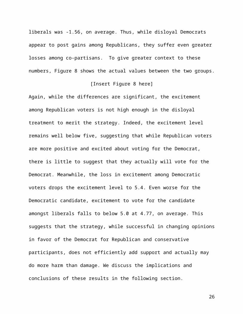
Figure 5: Likert rating measuring Candidate Excitement

26

Figure 6: Difference in Means for Candidate Preference, Thermometer Score, and Excitement Score with 95% Confidence Interval

27

Error bars represent 95% confidence intervals. ** represents statistically significant difference in means P<.05 using two-tailed test

28

29

Figure 7: Difference in Thermometer Scores by Partisanship and Ideology

Democrats Republican0

10

20

30

40

50

60

70

80

90

76.42

24.57

63.24

38.77

Difference in Thermometer Ratings between Treatment 2 and Control

ControlTreatment 2

liberal conservative0

10

20

30

40

50

60

70

8072.27

26.99

58.41

38.14

Difference in Thermometer Ratings Between Treatment 2 and Control

ControlTreatment 2

30

Figure 8: Difference in Excitement Score by Partisanship and Ideology

Democrats Republicans0

1

2

3

4

5

6

7

86.93

1.27

5.4

2.25

Difference in Excitement Ratings Between Treatment 2 and Control

ControlTreatment 2

Liberals Conservatives0

1

2

3

4

5

6

76.34

1.51

4.77

2.38

Difference in Excitement Ratings Between Treatment 2 and Control

ControlTreatment 2

31

Appendix A: Summary of Differences Between The Treatment and Control Groups For Treated Respondents

Treatment 1 (Ambiguity) Treatment 2 (Disloyal)Candidate PreferenceParty IDDemocrat -.02 -.02Independent .03 -.16**Republican -0.01 -.08**IdeologyLiberal -.03 -.04*Moderate .06 -.02Conservative -.03 -.14**State TypeBlue State .09** .06Red State -.12** -.14**Purple State .06 -.08Thermometer RatingParty IDDemocrat -2.09 -13.18**Independent -2.01 -1.92Republican .35 14.21**IdeologyLiberal -2.73 -13.86**Moderate -.71 .96Conservative -.35 11.15**State TypeBlue State -6.26** -10.52**Red State 6.31* 1.31Purple State -7.04* -2.45Excitement ScoreParty IDDemocrat -.32 -1.53**Independent -.48 -.48Republican .13 .99**IdeologyLiberal -.34 -1.57**Moderate -.49 -.44Conservative .11 .87**State TypeBlue State -.65** -1.43**Red State .52 -.07Purple State -.66 -.66* P<.1, **P<.05

32

Appendix B: Summary of Differences Between The Treatment and Control Groups For All RespondentsTreatment 1 (Ambiguity) Treatment 2 (Disloyal)

Candidate PreferenceParty IDDemocrat -.02 -.02Independent .05 -.13**Republican .01 -.03IdeologyLiberal -.03 -.05Moderate .04 -.02Conservative 0 -.11State TypeBlue State .8* .04Red State -.12** -.11**Purple State .04 .07Thermometer RatingParty IDDemocrat -.35 -8.01**Independent -1.98 -1.47Republican -1.05 9.89**IdeologyLiberal -.62 -8.83**Moderate 1.12 -.3Conservative -1.69 9.67**State TypeBlue State -4.16* -7.22**Red State 6.7* 2.4Purple State -5.38 -1.0Excitement ScoreParty IDDemocrat -.06 -.83**Independent -.57 -.4Republican -.14 .65**IdeologyLiberal 0 -.9**Moderate -.37 -.32Conservative -.1 .87**State TypeBlue State -.42 -.94**Red State .65* .19Purple State -.69* -.28* P<.1, **P<.05

33