wp_18279

5/16/2018 wp_18279 - slidepdf.com

http://slidepdf.com/reader/full/wp18279 1/22

WHITE PAPER

Risk Aggregation and Economic Capital

5/16/2018 wp_18279 - slidepdf.com


The content provider or this paper was Jimmy Skoglund, Risk Expert at SAS. [email protected]

5/16/2018 wp_18279 - slidepdf.com

http://slidepdf.com/reader/full/wp18279 3/22i


Table of Contents

Introduction .....................................................................................................2Risk Aggregation Methodologies ....................................................................3

Linear Risk Aggregation ...............................................................................3

Copula-Based Risk Aggregation ..................................................................5

Overview o Copulas ....................................................................................5

Measuring Copula Dependence ...................................................................7

The Normal and t Copulas ...........................................................................9

Normal Mixture Copulas ............................................................................11

Aggregate Risk Using Copulas ...................................................................11

Capital Allocation ..........................................................................................12

Defning Risk Contributions .......................................................................13

Issues in Practical Estimation o Risk Contributions .................................15

Value-Based Management Using Economic Capital ....................................16

Conclusion .....................................................................................................17

Reerences .....................................................................................................18

5/16/2018 wp_18279 - slidepdf.com



Introduction

The ollowing paper discusses challenges aced by fnancial institutions in the areas

o risk aggregation and economic capital. SAS has responded to these challenges

by delivering an integrated risk oering, SAS® Risk Management or Banking. The

solution meets the immediate requirements banks are looking or, while providing a

ramework to support uture business needs.

Risk management or banks involves risk measurement and risk control at the

individual risk level, including market risk or trading books, credit risk or trading

and banking books, operational risks and aggregate risk management. In many

banks, aggregate risk is defned using a rollup or risk aggregation model; capital,

as well as capital allocation, is based on the aggregate risk model. The aggregate

risk is the basis or defning a bank’s economic capital, and is used in value-based

management such as risk-adjusted perormance management.

In practice, dierent approaches to risk aggregation can be considered to be either

one o two types: top-down or bottom-up aggregation. In the top-down aggregation,

risk is measured on the sub-risk level such as market risk, credit risk and operational

risk; subsequently, risk is aggregated and allocated using a model o risk aggregation.

In the bottom-up aggregation model, the sub-risk levels are aggregated bottom-up

using a joint model o risk and correlations between the dierent sub-risks that drive

risk actors. In this method the dierent risk actors or credit, market, operational risk,

etc. are simulated jointly.

While bottom-up risk aggregation may be considered a preerred method orcapturing the correlation between sub-risks, sometimes bottom-up risk aggregation

is difcult to achieve because some risks are observed and measured at dierent

time horizons. For example, trading risk is measured intraday or at least daily while

operational risk is typically measured yearly. The difculty in assigning a common

time horizon or risks that are subject to integration does not necessarily become

easier using a top-down method. Indeed, this method also requires sub-risks

to be measured using a common time horizon. However, a distinctive dierence

between the approaches is that or the top-down method, one is usually concerned

with speciying correlations on a broad basis between the dierent sub-risks (e.g.,

correlation between credit and market risk or correlation between operational risk

and market risk). In contrast, the bottom-up approach requires the specifcation o all

the underlying risk drivers o the sub-risks. Such detailed correlations may be natural

to speciy or some sub-risks such as trading market and credit risk, but not or

others such as operational risk and trading risk. In those cases, the broad correlation

specifcation approach in top-down approaches seems easier than speciying the ull

correlation matrix between all risk drivers or trading risk and operational risk.

Current risk aggregation models in banks range rom very simple models that add

sub-risks together to linear risk aggregation, and in some cases, risk aggregation

using copula models. Also, some banks may use a combination o bottom-up and

top-down approaches to risk integration.

2

5/16/2018 wp_18279 - slidepdf.com



Recently Basel (2008) addressed risk aggregation as one o the more challenging

aspects o banks’ economic capital models. Recognizing that there has been some

evolution in banks’ practices in risk aggregation, Basel noted that banks’ approaches

to risk aggregation are generally less sophisticated than sub-risk measurementmethodology. One o the main concerns in risk aggregation and calculation o

economic capital is their calibration and validation – requiring a substantial amount o

historical time-series data. Most banks do not have the necessary data available and

may have to rely partially on expert judgment in calibration.

Following the importance o risk aggregation in banks’ economic capital models,

there is vast literature on top-down risk aggregation. For example, Kuritzkes,

Schuermann and Weiner (2002) consider a linear risk aggregation in fnancial

conglomerates such as bancassurance. Rosenberg and Schuermann (2004) study

copula-based aggregation o banks’ market, credit and operational risks using a

comparison o the t- and normal copula. See also Dimakos and Aas (2004) and

Cech (2006) or comparison o the properties o dierent copula models in top-down

risk aggregation.

Risk Aggregation Methodologies

Risk aggregation involves the aggregation o individual risk measurements using

a model or aggregation. The model or aggregation can be based on a simple

linear aggregation or using a copula model. The linear aggregation model is

based on aggregating risk, such as value at risk (VaR) or expected shortall (ES),

using correlations and the individual VaR or ES risk measures. The copula model

aggregates risk using a copula or the co-dependence, such as the normal or

t-copula, and the individual risk’s proft and loss simulations. The copula model

allows greater exibility in defning the dependence model than the linear risk

aggregation. Below we review both o these approaches to risk aggregation.

Linear Risk Aggregation

The linear model or risk aggregation takes the individual VaR or ES risks as inputs

and aggregates the risks using the standard ormula or covariance. That is,

3

5/16/2018 wp_18279 - slidepdf.com



where is the correlation between risks i and j and α is the confdence level o

the aggregate VaR. In this model there are two extreme cases. That is, the zero-

correlation aggregate VaR,

and the maximum correlation VaR ( =1 or all i, j)

The maximum correlation model is reerred to as the simple summation model

in Basel (2008). More generally, the linear risk aggregation can be perormed or

economic capital measure, EC, such that or EC risks EC1,..., ECn we have

Table 1 displays an example risk aggregation using the linear risk aggregation model.

The sub-risks are market risk, credit risk, operational risk, unding risk and other risks

(e.g., business risks). In the correlated risk aggregation, we have used the correlation

matrix

between the risks. The independent aggregate risk is obtained using zero

correlations and the additive risk is obtained using correlations equal to unity.

Finally, we also calculate the actual contribution risk as a percentage o total risk.

The contribution is the actual risk contribution rom the sub-risks obtained in the

context o the portolio o total risks1. This risk contribution is oten compared with

standalone risk to obtain a measure o the diversifcation level. For example, the

market risk sub-risk has a standalone risk share o 16,3 percent whereas the risk

contribution share is 11,89 percent. This represents a diversifcation level o about

73 percent compared to the simple summation approach.

Table 1: Risk aggregation using the linear risk aggregation model.

Sub-Risks Aggregated

RiskIndependent

Risk Additive

RiskContribution

Risk (%)

Total Risk 1524,85 1125,70 2013,00 100,0

Market Risk 250 250 250 11,89

Credit Risk 312 312 312 12,37

Operational Risk 119 119 119 3,03

1 In the section on capital allocation, we defne the risk contribution as the derivative o total risk withrespect to the sub-risks. That is, the derivative o with respect to risk exposure i.

4

5/16/2018 wp_18279 - slidepdf.com



Sub-Risks Aggregated

RiskIndependent

Risk Additive

RiskContribution

Risk (%)

Funding Risk 345 345 345 11,31

Other Risks 987 987 987 61,40

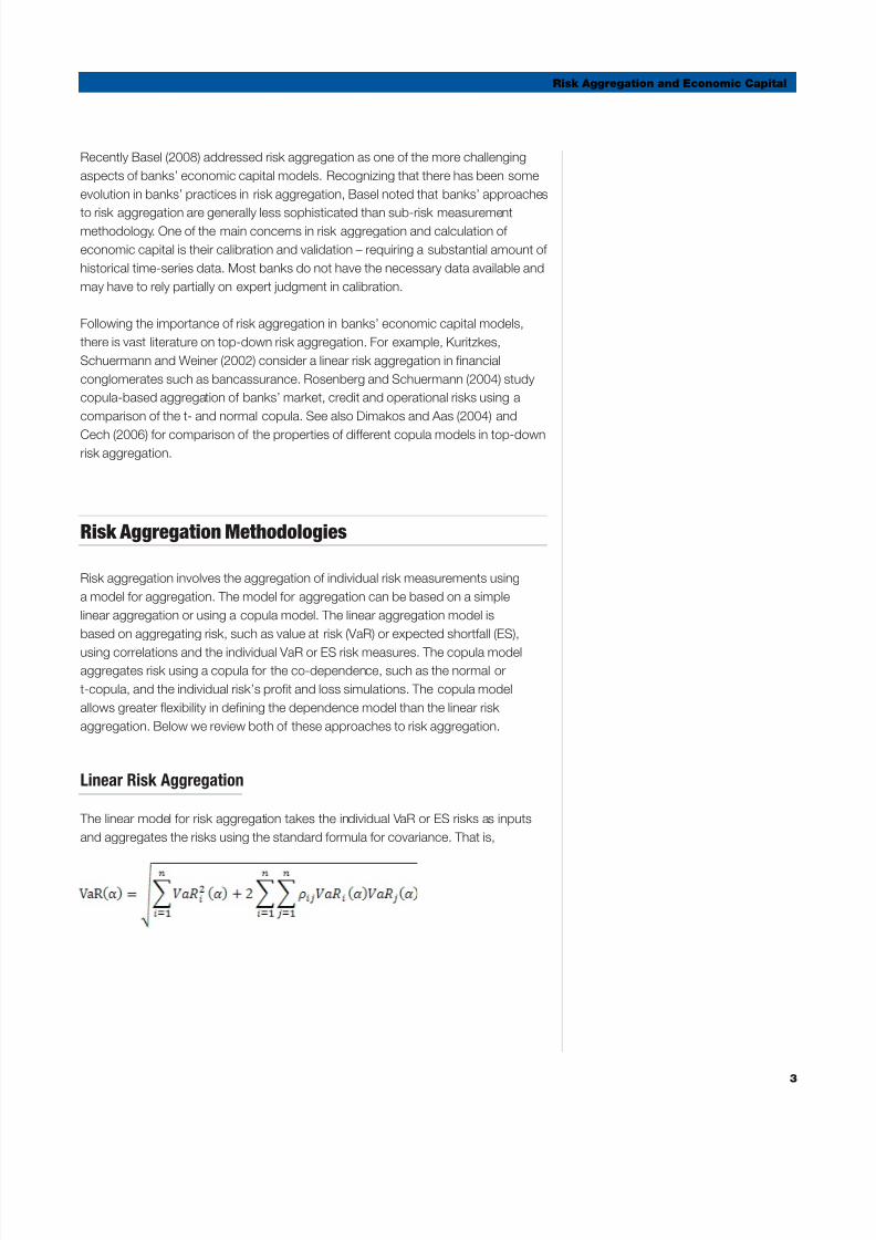
The linear model o risk aggregation is a very convenient model to work with. The only

data required is the estimates o the sub-risks’ economic capital and the correlation

between the sub-risks. However, the model also has some serious drawbacks. For

example, the model has the assumption that quantiles o portolio returns are the same

as quantiles o the individual return – a condition that is satisfed in case the total risks

and the sub-risks come rom the same elliptic density amily 2.

The linear risk aggregation model is the aggregation model used in the new solvency

regulations or the standard approach.

Copula-Based Risk Aggregation

While linear risk aggregation only requires measurement o the sub-risks, copula

methods o aggregation depend on the whole distribution o the sub-risks. One

o the main benefts o copula is that it allows the original shape o the sub-risk

distributions to be retained. Further, the copula also allows or the specifcation

o more general dependence models than the normal dependence model.

Overview o Copulas

To get a rough classifcation o available copulas, divide them into elliptic copulas

(which are based on elliptic distributions), non-elliptic parametric copulas and

copulas consistent with the multivariate extreme value theory. There are also other

constructions based on transormations o copulas, including copulas constructed

by using Bernstein polynomials. (See Embrechts et al. (2001) and Nelsen (1999) or

an overview o dierent copulas.)

Implicit in the use o copulas as a model o co-dependence is the separation o the

univariate marginal distributions modeling and the dependence structure. In this

setting, the model specifcation ramework consists o two components that can be

constructed, analyzed and discussed independently. This gives a clear, clean, exibleand transparent structure to the modeling process.

2 See Rosenberg and Schuermann (2004) or a derivation o the linear aggregation model and itsspecial case o aggregating the multivariate normal distribution.

5

5/16/2018 wp_18279 - slidepdf.com



When introducing copulas, we start with the distribution unction o the variables,

X1,X2,...Xn ,

The copula is then simply the distribution o the uniorms. That is,

For example, this means that a two-dimensional copula, C, is a distribution unction

on the unit square [0,1]´[0,1] with uniorm marginals.

Figure 1 displays three dierent two-dimensional copulas: the perect negative

dependence copula (let panel); the independence copula (middle panel); and the

perect dependence copula (right panel). The perect negative dependence copula

has no mass outside the northeast corner, whereas the perect dependence copula

has no mass outside the diagonal. In contrast, the independence copula has mass

almost everywhere.

Figure 1: Some special copulas: the perect negative dependence (let panel); the

independence copula (middle panel); and the perect dependence copula (right panel).

Since the copula is defned as the distribution o the uniorm margins, the copula or a

multivariate density unction can be obtained using the method o inversion. That is,

where C(u,v) is the copula, u and v are uniorms, Fx,y is the joint cumulative density

unction, and Fx–1

and Fy–1

are the inverse marginal quantile unctions. In the specialcase that the joint and the marginal densities and copula are normal, the relationship

can be written as:

where ϕ is the normal cumulative density and ϕ is the normal marginal density.

6

5/16/2018 wp_18279 - slidepdf.com



7

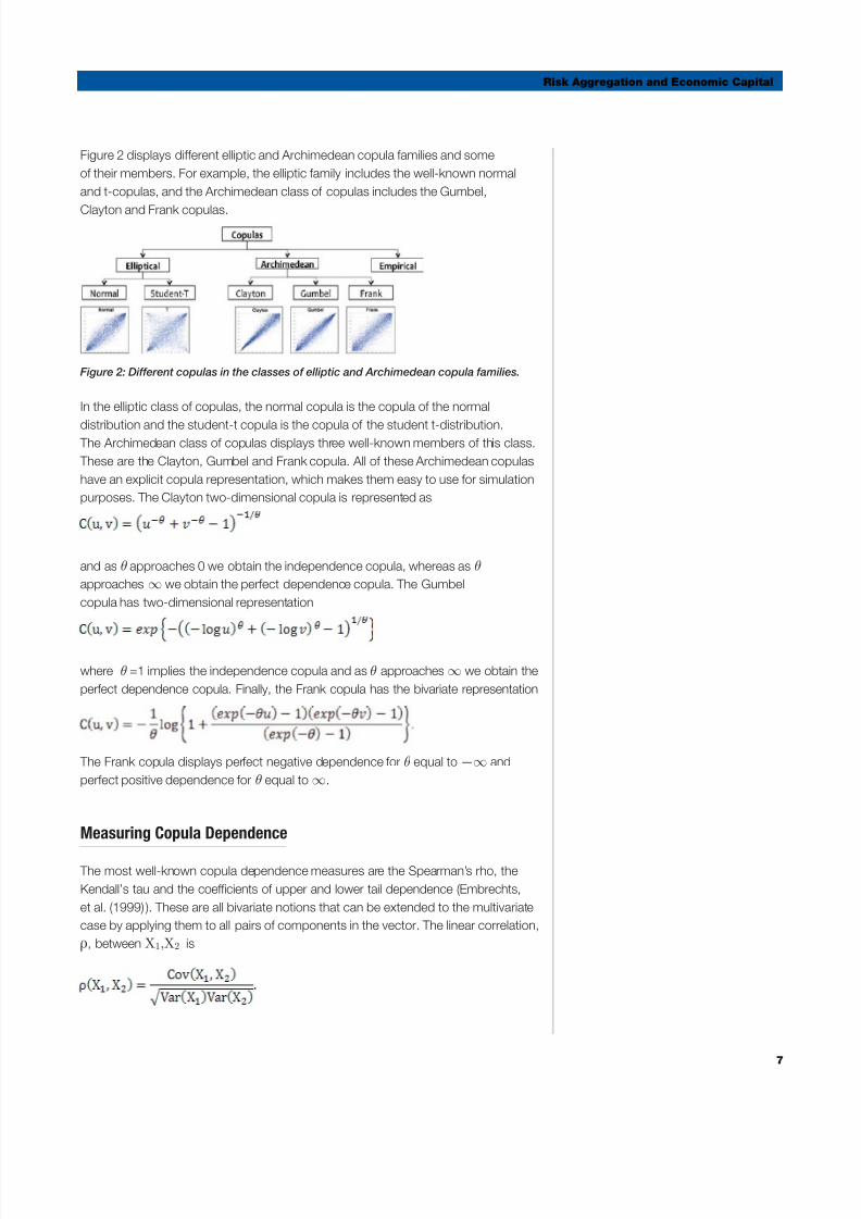
Figure 2 displays dierent elliptic and Archimedean copula amilies and some

o their members. For example, the elliptic amily includes the well-known normal

and t-copulas, and the Archimedean class o copulas includes the Gumbel,

Clayton and Frank copulas.

Figure 2: Dierent copulas in the classes o elliptic and Archimedean copula amilies.

In the elliptic class o copulas, the normal copula is the copula o the normal

distribution and the student-t copula is the copula o the student t-distribution. The Archimedean class o copulas displays three well-known members o this class.

These are the Clayton, Gumbel and Frank copula. All o these Archimedean copulas

have an explicit copula representation, which makes them easy to use or simulation

purposes. The Clayton two-dimensional copula is represented as

and as θ approaches 0 we obtain the independence copula, whereas as θ

approaches ∞ we obtain the perect dependence copula. The Gumbel

copula has two-dimensional representation

where θ =1 implies the independence copula and as θ approaches ∞ we obtain the

perect dependence copula. Finally, the Frank copula has the bivariate representation

The Frank copula displays perect negative dependence or θ equal to —∞ and

perect positive dependence or θ equal to ∞.

Measuring Copula Dependence

The most well-known copula dependence measures are the Spearman’s rho, the

Kendall’s tau and the coefcients o upper and lower tail dependence (Embrechts,

et al. (1999)). These are all bivariate notions that can be extended to the multivariate

case by applying them to all pairs o components in the vector. The linear correlation,

ρ, between X1,X2 is

5/16/2018 wp_18279 - slidepdf.com



8

Linear correlation is, as the word indicates, a linear measure o dependence.

For constants α,β,c1,c2 it has the property that

and hence is invariant under strictly increasing linear transormations. However,

in general

or strictly increasing transormations, F1 and F2 and hence ρ is not a copula

property as it depends on the marginal distributions.

For two independent vectors o random variables with identical distribution unction,

(X1,X2 ) and(X∼

1,X∼

2 ), Kendall’s tau is the probability o concordance minus the

probability o discordance, i.e.,

Kendall’s tau, τ, can be written as

and hence is a copula property. Spearman’s rho is the linear correlation o the

uniorm variables u=F1(X1 ) and v= F1(X2 ) i.e.,

and the Spearman’s rho, ρS, is also a property o only the copula C and not the

marginals. Oten the Spearman’s rho is reerred to as the correlation o ranks. We

note that Spearman’s rho is simply the usual linear correlation, ρ, o the probability-

transormed random variables.

Another important copula quantity is the coefcient o upper and lower tail

dependence. The coefcient o upper tail dependence ΛU(X1,X2 ) is defned by

provided that the limit ΛU(X1,X2 )∈[0,1] exists. The coefcient o lower tail

dependence,ΛU(X1,X2 ), is similarly defned by

5/16/2018 wp_18279 - slidepdf.com



9

provided that the limit ΛL(X1,X2 )∈[0,1] exists. I ΛU(X1,X2 )∈(0,1], then X1 and X2

are said to have asymptotic upper tail dependence. I ΛU(X1,X2 )=0, then X1 and X2

are said to have asymptotic upper tail independence. The obvious interpretation o

the coefcients o upper and lower tail dependence is that these numbers measurethe probability o joint extremes o the copula.

The Normal and t Copulas

The Gaussian copula is the copula o the multivariate normal distribution.

The random vector X=(X1,..., X1 ) is multivariate normal i and only i the

univariate margins F1,..., F1 are Gaussians and the dependence structure

is described by a unique copula unction C, the normal copula, such that

where ϕ is the standard multivariate normal distribution unction with linear

correlation matrix Σ and φ–1 is the inverse o standard univariate Gaussian distribution

unction. For the Gaussian copula there is an explicit relation between the Kendall’s

tau, τ, the Spearman’s rho, ρS, and the linear correlation, ρ, o the random variables

X1,X2. In particular,

The copula o the multivariate student t distribution is the student t copula.Let X be a vector with an n-variate student t distribution with ν degrees o reedom,

mean vector μ (or ν>1) and covariance matrix (ν /(ν-2))Σ (or ν>2). It can be

represented in the ollowing way:

where μ∈Rn,S∼χ²(v) and the random vector Z∼N(0,Σ ) is independent o S. The

copula o the vector X is the student t copula with ν degrees o reedom. It can

be analytically represented as

where tn denotes the multivariate distribution unction o the random vector

and tv–1 denotes the inverse margins o tn. For the bivariate t copula, there is an

explicit relation between the Kendall’s tau and the linear correlation o the random

variables X1,X2. Specifcally,

5/16/2018 wp_18279 - slidepdf.com



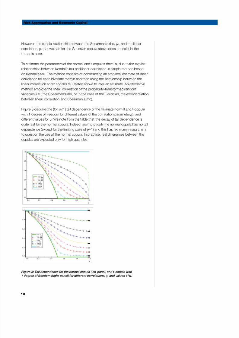
However, the simple relationship between the Spearman’s rho, ρS, and the linear

correlation, ρ, that we had or the Gaussian copula above does not exist in the

t-copula case.

To estimate the parameters o the normal and t-copulas there is, due to the explicit

relationships between Kendall’s tau and linear correlation, a simple method based

on Kendall’s tau. The method consists o constructing an empirical estimate o linear

correlation or each bivariate margin and then using the relationship between the

linear correlation and Kendall’s tau stated above to iner an estimate. An alternative

method employs the linear correlation o the probability-transormed random

variables (i.e., the Spearman’s rho, or in the case o the Gaussian, the explicit relation

between linear correlation and Spearman’s rho).

Figure 3 displays the (or u≤1) tail dependence o the bivariate normal and t-copula

with 1 degree o reedom or dierent values o the correlation parameter, ρ, and

dierent values or u. We note rom the table that the decay o tail dependence is

quite ast or the normal copula. Indeed, asymptotically the normal copula has no tail

dependence (except or the limiting case o ρ=1) and this has led many researchers

to question the use o the normal copula. In practice, real dierences between the

copulas are expected only or high quantiles.

Figure 3: Tail dependence or the normal copula (let panel) and t-copula with

1 degree o reedom (right panel) or dierent correlations, ρ , and values o u.

5/16/2018 wp_18279 - slidepdf.com



11

Normal Mixture Copulas

A normal mixture distribution is the distribution o the random vector

where f(W)∈Rn,W ≥0 is a random variable and the random vector ∼N(0,Σ ) is

independent o W . In particular, i f(W)=μ∈Rn andW is distributed as an inverse

gamma with parameters ((1/2)v,(1/2)v), then X is distributed as a t-distribution.

Another type o normal mixture distribution is the discrete normal mixture distribution,

where f(W)=μ andW is a discrete random variable taking values w1, w2 with

probability p1, p2. By setting w2 large relative to w1 and p1 large relative to p2, one

can interpret this as two states – one ordinary state and one stress state. The normal

mixture distribution where f(W)=μ+W ϒ and γ is dierent among at least one o

the components γ1,...,γ1 is a non-exchangeable normal mixture distribution, and

γ is called an asymmetry parameter. Negative values o γ produce a greater level

o tail dependence or joint negative returns. This is the case that is perceived as

relevant or many fnancial time series where joint negative returns show stronger

dependence than joint positive returns. The copula o a normal mixture distribution

is a normal mixture copula.

Aggregate Risk Using Copulas

When aggregating risk using copulas, the ull proft and loss density o the sub-

risks, as well as the choice o copula and copula parameter(s), is required. This is

only marginally more inormation than is required or the linear aggregation model.

In particular, or the linear risk aggregation model we only needed the risk measureso the sub-risks. Using a copula model or aggregation, additional correlation

parameters may be required (e.g., or the student t-copula we also require a degree

o reedom parameter).

5/16/2018 wp_18279 - slidepdf.com



In Table 2 below, we calculate value at risk (VaR) and expected shortall (ES) copula

aggregations using the normal, t-copula and normal mixture copula or a 99 percent

confdence level. The risk aggregation using the normal mixture copula is evaluated

using a bivariate mixture with parameterization NMIX(p1,p2,x1,x2). Here, p1 andp2 are the probabilities o normal states 1 and 2 respectively and x1, x2 are the

mixing coefcients. The individual risk’s proft and loss distributions are simulated

rom standard normal densities, and the correlated aggregation correlation matrix

is the same as the one used or Table 1 above3. Table 2 shows that the copula risk

aggregation VaR and ES increase when a non-normal copula model, such as the

t-copula or the normal mixture copula, is used or aggregation. For the t-copula, the

aggregate risk generally increases the lower the degrees o reedom parameter, and

or the normal mixture copula, the aggregate risk generally increases with the mixing

coefcient. For a more detailed analysis o these copula models in the context o

bottom-up risk aggregation or market risk, we reer to Skoglund, Erdman and

Chen (2010).

Table 2: Copula value at risk and expected shortfall risk aggregation

using the normal copula, t-copula and the normal mixture copula.

Copula Model Aggregate VaR (99%) Aggregate ES (99%)

Normal 7,74 8,70

T(10) 7,93 9,28

T(5) 8,16 9,67

NMIX(0,9,0.1,1,10) 8,06 9,94

NMIX(0,9,0.1,1,400) 8,91 10,82

Capital Allocation

Having calculated aggregate risk using a method o risk aggregation, the next step is

to allocate risks to the dierent sub-risks. In particular, banks allocate risk/capital or

the purpose o:

• Understanding the risk profle o the portolio.

• Identiying concentrations.

• Assessing the efciency o hedges.

• Perorming risk budgeting.

• Allowing portolio managers to optimize portolios based on risk-adjusted

perormance measures.

3 The act that the individual proft and loss distributions are simulated rom the standard normaldistribution is without loss o generality. In principle, the underlying proft and loss distributionscan be simulated rom any density.

5/16/2018 wp_18279 - slidepdf.com



13

In practice, capital allocation is based on risk contributions to risk measures such

as aggregate economic capital. In order to achieve consistency in risk contributions

when economic capital model risks dier rom actual capital, banks regularly scale

economic capital risk contributions to ensure risk contributions equal the sum o totalcapital held by the bank.

Defning Risk Contributions

Following Litterman (1996) – introducing the risk contributions in the context o the

linear normal model – there has been a ocus on risk contribution development

or general non-linear models. Starting with Hallerbach (1998), Tasche (1999) and

Gourieroux et al. (2000), general value at risk and expected shortall contributions

were introduced. These contributions utilize the concept o the Euler allocation

principle. This is the principle that a unction, ψ, that is homogenous o degree 1

and continuously dierentiable satisfes

That is, the sum o the derivative o the components o the unction, ψ, sum to the

total. I we interpret ψ as a risk measure and wi as the weights on the sub-risk’s,

then the Euler allocation suggests that risk contributions are computed as frst-order

derivatives o the risk with respect to the sub-risk’s.

The Euler allocation is a theoretically appealing method o calculating risk

contributions. In particular, Tasche (1999) shows that this is the only method that

is consistent with local portolio optimization. Moreover, Denault (2001) shows that

the Euler decomposition can be justifed economically as the only “air” allocation in

co-operative game theory (see also Kalkbrener (2005) or an axiomatic approach to

capital allocation and risk contributions). These properties o Euler risk contributions

have led to the Euler allocation as the standard metric or risk; it’s also used by

portolio managers or risk decomposition into subcomponents such as instruments

or sub-risks. Recently, Tasche (2007) summarized the to-date fndings and best-

practice usage o risk contributions based on Euler allocations; Skoglund and Chen

(2009) discussed the relation between Euler risk contributions and so-called risk

actor inormation measures4.

4 Risk actor inormation measures attempt to break down risk into the underlying risk actors suchas equity, oreign exchange and commodity. The risk actor inormation measure is in general not adecomposition in the sense o risk contributions.

5/16/2018 wp_18279 - slidepdf.com



In the copula risk aggregation, the input or the sub-risks is a discrete simulation o

profts and losses. Hence, strictly, the derivative o aggregate risk with respect to

the sub-risks does not exist. How do we defne risk decomposition in this case?

The answer lies in the interpretation o risk contributions as conditional expectations(see Tasche (1999), Gourieroux et al. (2000)). This means that we can estimate

VaR contributions or the copula risk aggregation technique using the conditional

expectation

where this is the risk contribution or sub-risk i, L is the aggregate loss and Li is the

loss o sub-risk i. The expected shortall (ES) risk measure is defned as the average

loss beyond VaR. That is,

Hence, taking the expectation inside the integral, ES risk contributions can be

calculated as conditional expectations o losses beyond VaR.

Table 3 below illustrates the computation o discrete risk contributions using an

example loss matrix. In particular i the tail scenario 5 corresponds to the aggregate

VaR, that is 39,676, then the VaR contributions or the sub-risks correspond to

the realized loss in the sub-risks corresponding VaR scenario. Specifcal ly, the

VaR contribution or sub-risk 1 is then -0,086, the VaR contribution or sub-risk

2 is 44,042 and or sub-risk 3 is -1,975. By defnition these contributions sum to

aggregate VaR. The ES is defned as the expected loss beyond VaR and is hence

the average o aggregate losses beyond VaR. This average is, rom Table 3, 90,9.

The ES contributions are respectively or sub-risk 1, 2 and 3: 0,1107, 90,74, and0,0945. These contributions are obtained by averaging the sub-risks’ corresponding

ES scenarios or tail scenario 1, 2, 3 and 4. Again, as in the VaR case, the sum o ES

contributions equals the aggregate ES.

Table 3: Example loss scenarios or aggregate risk and sub-risks 1, 2 and 3, and the

computation o VaR and ES risk contributions.

TailScenario

Sub-Risk 1Loss

Sub-Risk 2Loss

Sub-Risk 3Loss

AggregateLoss

1 0,701 101,73 0,727 103,158

2 -0,086 101,365 0,453 101,732

3 -0,086 87,150 1,073 88,137

4 -0,086 72,572 -1,875 70,611

5 (VaR) -0,086 44,043 -4,281 39,676

5/16/2018 wp_18279 - slidepdf.com



15

Having calculated risk contributions, the next step is to allocate capital. Since actual

capital may not be equal to aggregated risk, a scaling method is used. That is, the

capital contribution is obtained by scaling the risk contribution by the capital and

aggregate risk ratio.

Issues in Practical Estimation o Risk Contributions

When estimating risk contributions, it is important that the risk contributions are stable

with respect to small changes in risk; otherwise, the inormation about the sub-risks

contribution to aggregate risk will not be meaningul. Indeed, i small changes in risk

yield large changes in risk contributions then the amount o inormation about the

risk contained in the risk contributions is very small. More ormally, we may express

this requirement o risk smoothness by saying that the risk measure must be convex.

Artzner et al. (1999) introduces the concept o coherent risk measures. A coherent risk

measure, m, has the property that:

m(X+Y)<=m(X)+m(Y) (subadditive)

m(tX)=tp(X) (homogenous o degree one)

I X>Y a.e. then m(X)>m(Y) (monotonous)

m(X+a)=m(X)+a (risk-ree condition).

The frst and the second condition together imply that the risk measure is convex.

Unortunately VaR is not a convex risk measure in general; in particular, this implies

that the VaR contributions may be non-smooth and erratic.

Figure 5 displays the VaR measure (y-axis) when the position (x-axis) is changed.

Notice that the VaR curve is non-convex and non-smooth. Considering the

calculations o VaR contributions in this case may be misleading, as the VaR

contributions change wildly even or small changes in underlying risk position.

Figure 5: VaR is in general a non-convex risk measure such that the risk profle

is non-convex (i.e., non-smooth).

5/16/2018 wp_18279 - slidepdf.com



The above properties o VaR contributions have led many practitioners to work

with expected shortall, and in particular, risk contributions to expected shortall. In

contrast to VaR, expected shortall is a coherent risk measure and hence can be

expected to have smooth risk contributions. Alternatively, VaR is used as the riskmeasure while risk contributions are calculated using expected shortall risk and

subsequently scaled down to match aggregate VaR. Other approaches to smoothing

VaR contributions include averaging the losses close to the VaR point, or smoothing

the empirical measure by Kernel estimation (Epperlein and Smillie (2006)).

Risk contributions are also key in a bank’s approach to measuring and managing

risk concentrations. In particular, a bank’s ramework or concentration risk and

limits should be well-defned. In Tasche (2006), Memmel and Wehn (2006); Garcia,

Cespedes et al. (2006); and Tasche (2007), the ratio o Euler risk contribution

to the standalone risk is defned as the diversifcation index. For coherent risk

measures, the diversifcation index measures the degree o concentration such

that a diversifcation index o 100 percent or a sub-risk may be deemed to have ahigh risk concentration. In contrast, a low diversifcation index, say 60 percent, may

be considered to be a well-diversifed sub-risk. Note that the diversifcation index

measures the degree o diversifcation o a sub-risk in the context o a given portolio.

That is, the risk, as seen rom the perspective o a given portolio, may or may not be

diversifed.

Value-Based Management Using Economic Capital

The economic capital and the al location o economic capital is used in a bank’sperormance measurement and management to distribute the right incentives

or risk-based pricing, ensuring that only exposures that contribute to the bank’s

perormance targets are considered or inclusion in the portolio. In principle, banks

add an exposure to a portolio i the new risk-adjusted return is greater than the

existing, i.e.

Here, RCn+1, is the risk contribution o the new exposure with respect to economic

capital and rn+1 is the expected return o the new exposure. Value is created, relative

to the existing portolio, i the above condition is satisfed. For urther discussion

on risk-adjusted perormance management or traditional banking book items,

see the SAS white paper Funds Transfer Pricing and Risk-Adjusted Performance

Measurement.

5/16/2018 wp_18279 - slidepdf.com



17

About SAS® Risk Management for Banking

SAS Risk Management or Banking has been designed as a comprehensive

and integrated suite o quantitative risk management applications, combining

market risk, credit risk, asset and liability management, and frmwide risks into

one solution. The solution leverages the underlying SAS 9.2 platorm and the

SAS Business Analytics Framework, providing users with a exible and modular

approach to risk management. Users can start with one o the predefned

workows and then customize or extend the unctionality to meet ever-changing

risk and business needs. The introduction o SAS Risk Management or Banking

will take the industry’s standards to a higher paradigm o analytics, data

integration and risk reporting.

Conclusion

Risk aggregation and estimation o overall risk is key in banks’ approaches to

economic capital and capital allocation. The resulting capital also orms the basis or

banks’ value-based management o the balance sheet.

When estimating aggregate capital, one typically uses a combination o bottom-up

and top-down risk aggregation approaches. The top-down approach to risk capital

involves the selection o the aggregation model, such as the linear aggregation

or copula aggregation model, and the estimation o the dependence between

aggregate risks using historical and/or expertise data. For the linear risk aggregation

model, the correlations between the risks and the individual risk levels are needed

or risk aggregation. The copula aggregation model, being a more general approach

to risk aggregation, uses inormation about the complete proft and loss density o

the underlying risks and typically requires additional parameters to correlation to ully

capture dependence between risks. In practice, both approaches have their own

drawbacks and benefts. It is thereore advisable to consider multiple approaches to

risk aggregation.

This SAS white paper has presented the linear and copula model approaches to

the calculation o risk aggregations and economic capital. We have also discussed

the use o risk contributions as a basis or allocating economic capital. Finally, we

demonstrated how to integrate economic capital into risk adjusted perormance.

5/16/2018 wp_18279 - slidepdf.com



References

Artzner, P., F. Delbaen, J.-M. Eber and D. Heath, 1999. Coherent Measures o 1.

Risk. Mathematical Finance 9 (3): 203-228.

Cech, C., 2006.2. Copula-Based Top-Down Approaches in Financial Risk

Aggregation. University o Applied Sciences Vienna, Working Paper Series No.

32.

Denault, M., 2001. Coherent Allocation o Risk Capital,3. Journal of Risk , 4(1).

Dimakos, X. and K. Aas, 2004. Integrated Risk Modelling.4. Statistical Modelling

4: 265-277.

Embrechts, P., A. McNeil and D. Straumann, 1999. Correlation and Dependence5.in Risk Management: Properties and Pitalls. Risk Management: Value at Risk

and Beyond . Edited by M. Dempster and H.K. Moatt. Cambridge: Cambridge

University Press.

Embrechts, P., F. Lindskog and A. McNeil, 2001.6. Modelling Dependence with

Copulas and Applications to Risk Management, a working paper. RiskLab,

Zurich.

Epperlein, E. and A. Smillie, 2006. Cracking VaR with Kernels.7. Risk , 70-74.

Garcia, J., J. Herrero, A. Kreinin and D. Rosen, 2006. A Simple Multiactor8.

“Factor Adjustment” or the Treatment o Credit Capital Diversifcation. Journal of Credit Risk 2(3): 57-85.

Gourieroux, C., J.P. Laurent, and O. Scaillet, 2000. Sensitivity Analysis o Values9.

at Risk. Journal of Empirical Finance 7: 225-245.

Hallerbach, W., 1998. Decomposing Portolio Value at Risk: A General Analysis,10.

a working paper. Erasmus University, Rotterdam.

Kalkbrener, M., 2005. An Axiomatic Approach to Capital Allocation.11.

Mathematical Finance.

Kuritzkes, A., T. Schuermann and S. Weiner, 2002. Risk Measurement,12. Risk

Management and Capital Adequacy in Financial Conglomerates, a Wharton

paper.

Litterman, R., 1996. Hot Spots and Hedges.13. The Journal of Portfolio

Management 22: 52-75.

Memmel, C. and C. Wehn, 2005. The Supervisor’s Portolio: The Market Price14.

o Risk o German Banks rom 2001 to 2004 – Analysis and Models or Risk

Aggregation. Journal of Banking Regulation 7: 309-324.

5/16/2018 wp_18279 - slidepdf.com



19

Nelsen, R., 1999.15. An Introduction to Copulas. Springer Verlag.

Rosenberg, J. and T. Schuermann, 2004.16. A General Approach to Integrated

Risk Management with Skewed, Fat-Tailed Risks. Federal Reserve Bank o

New York, Sta Report No. 185.

Skoglund, J. and W. Chen, 2009. Risk Contributions, Inormation and Reverse17.

Stress Testing. Journal of Risk Model Validation 3(2): 40-60.

Skoglund, J., D. Erdman and W. Chen, 2010. The Perormance o Value-at-18.

Risk Models During the Crisis. Journal of Risk Model Validation 4(1): 1-23.

Skoglund, J., 2010.19. Funds Transfer Pricing and Risk-Adjusted Performance

Measurement, a SAS white paper. Available at http://www.sas.com/reg/wp/

corp/17624

Tasche, D., 1999.20. Risk Contributions and Performance Measurement,

a working paper. Technische Universität Munchen.

Tasche, D., 2006. Measuring Sectoral Diversifcation in an Asymptotic21.

Multi-Factor Framework. Journal of Credit Risk 2(3): 33-55.

Tasche, D., 2007.22. Euler Allocation: Theory and Practice. http://www.greta.it/

credit/credit2007/thursday/1_Tasche.pd.

5/16/2018 wp_18279 - slidepdf.com


SAS Institute Inc. World Headquarters +1 919 677 8000

To contact your local SAS ofce, please visit: www.sas.com/ofces

SAS and all other SAS Institute Inc. product or service names are registered trademarks or trademarks o SAS Institute Inc. in the USA

and other countries. ® indicates USA registration. Other brand and product names are trademarks o their respective companies.

Copyright © 2010, SAS Institute Inc. All rights reserved. 104545_S56228_0510

Documents

wp_18279