Embed Size (px)
Citation preview
Centre forComputationalFinance andEconomicAgents
WorkingPaperSeries
www.ccfea.net
WP068-13
Vince Vella andWing Lon Ng
Improving risk-adjustedperformance profile of intraday
trading models withNeuro-Fuzzy techniques and
moving averagehigh-frequency price signals
2013
Improving risk-adjusted performance profile of intraday
trading models with Neuro-Fuzzy techniques and moving
average high-frequency price signals
Vince Vellaa, Wing Lon Nga,∗
aCentre for Computational Finance and Economic Agents (CCFEA), University of Essex,Wivenhoe Park, Colchester CO4 3SQ, UK
Abstract
We present a performance comparison of risk-adjusted intraday trading strategiesbased on dynamic non-linear models using the more traditional Artificial Neu-ral Network, as well as Adaptive Neuro-Fuzzy Systems (ANFIS) and DynamicEvolving Neuro Fuzzy Systems (DENFIS). The model selection process takes intoaccount the risk-return measures together with flexible position holding periodsand a return band filter, employing a dynamic combination of moving averagesignals. Our results show that these models can be successfully applied to supportintraday trading strategies, especially when considering constraints such as trans-action costs and trading hours, which existing approaches in the literature do notaccount for.
Keywords: High-frequency trading, ANFIS, DENFIS, Feed-Forward Network,Dynamic Moving Average
1. Introduction
The profitability of trading rules is an incessant debate. Recent literature how-ever claims that profitability of technical trading rules has possibly moved to higherfrequency prices as a result of more efficient markets and faster algorithmic trading(Schulmeister, 2009). Notwithstanding this, other findings show that aggressivehigh-frequency trading (HFT) does not lead to the expected high excessive returns(Kearns et al., 2010). Whilst many former studies focuses on the application ofmodels solely to predict market movements (e.g. Son et al. (2012)), traders infinancial markets are typically interested in risk-adjusted performance rather than
∗Corresponding author. Tel.:0044-1206-874684Email addresses: [email protected] (Vince Vella), [email protected] (Wing Lon Ng)
Preprint submitted to Elsevier August 28, 2013
just price predictions themselves (Choey and Weigend, 1997; Xufre Casqueiro andRodrigues, 2006).
This paper provides new insights into the risk-adjusted performance of simpletechnical trading rules in an intraday stock trading scenario using high frequencydata with the application of artificial intelligence and soft computing techniques.Our first contribution is to present an analysis of the time-varying risk-adjustedperformance profile of the applied models by focusing on their dynamics over athe entire out-of-sample testing period and their daily cumulative performance.In contrast to common approaches in the literature which evaluates models usingrisk-return measures at an arbitrary single point in time (e.g. the end of thesample period), our goal is to provide a deeper understanding of the time-varyingperformance profile of the applied models.
Our second major contribution is the simple but yet effective extension ofcommon technical trading strategies by considering a ‘portfolio’ of moving averageprediction models controlled by neuro-fuzzy systems. This is further extended byapplying dynamic rules for return bands and trade position times. In line withTsang (2009) our models try to answer questions of the following form: “Willthe price go up (or down) by r% in the next t minutes?” We investigate theprofitability of models on less aggressive HFT, with holding periods between 10minutes and 1 hour, using 5 minute prices of a set of stocks listed on the LondonStock Exchange during the period 2007-2008. An important challenge in this studyis the choice of moving average window length. For example, if the price over aninterval is, in general, trending up, there are also several short-term downtrendsin the price data. Some of them are real trend reversal points and others arejust noise. The trend identifying mechanism should not be overly sensitive toshort-term fluctuations, hence applying a too short moving average, as that wouldresult in falsely reporting a break in trend. On the other hand, choosing a toolong moving average will result in late reaction to price movement. We suggest acombination of multiple moving average rules as input to the prediction models.
As a third contribution in this paper, we extend our trading systems with de-cision rules accounting for transaction costs and trading hours, and compare thetime series of risk adjusted performance measures obtained from different modeloptimisation functions such as risk-return functions, Root Mean Squared Error(RMSE) and models not considering transaction costs. When training and evalu-ating a trading system, most former studies only have very limited view of whatconstitutes successful investment decisions, defining on grounds of forecast accu-racy and win ratios, and often choose to minimise the forecast error of the priceprediction, setting this as the objective function (Alves Portela Santos et al., 2007;de Faria et al., 2009; Enke and Thawornwong, 2005; Medeiros et al., 2006). How-ever, a smaller forecast error does not necessarily translate into increased trading
2
profits (Brabazon and O’Neill, 2006). Recently, Krollner et al. (2010) find thatover 67% of the investigated studies use the forecast error as an evaluation met-ric and identify a lack of literature examining if machine learning techniques canimprove an investor’s risk-return trade-off. They also find that over 80% of thepapers report that their model outperformed the benchmark model, but most ofthem do not consider real world constraints at all (see also Alvarez Dıaz, 2010).
An interesting finding by Schulmeister (2009) was that by examining 30 minuteprices it was identified that beyond the 1990s the profitability of technical tradingrules has moved to higher frequency. He questioned that due to more efficientmarkets this might have moved to even higher frequencies for the more recentperiods.
Another finding in Tsai and Wang (2009) and Krollner et al. (2010) is thatArtificial Neural Networks (ANNs) are identified to be the dominant machinelearning technique in this area. On the downside ANNs are regarded as blackboxes that cannot describe the cause and effect. Moreover hybrid models wereagain found to provide better forecasts compared to ANNs used alone or traditionaltime series models. Following the emergence of Fuzzy Logic (Zadeh, 1975), Neuralnetworks and Fuzzy Inference Systems were brought together as general structuresfor approximating non-linear functions and dynamic processes. A popular citedtechnique in non stationary and chaotic time series prediction is the AdaptiveNeuro-Fuzzy Inference System (ANFIS) by Jang (1993). Successful application ofANFIS in trading applications by predicting stock price was demonstrated in Linet al. (2002); Gradojevic (2007); Kablan and Ng (2011) and many others, with thelatter study the only one identified that is focused on high frequency trading.
Equally important is the fact that to keep a successful trading edge these sys-tems have to adapt, and hence evolve, to address recurring and changing patternsin the intraday environment which are driven by the actions of informed and uni-formed traders. Implementing evolution requires an ability to balance learning andchanging while still respecting the past accumulated knowledge (Marsland, 2009).With a focus on dynamic learning of rules from data Kasabov and Song (2002)introduced pioneering work on evolving neuro fuzzy systems with the introductionof Evolving Neural-Fuzzy Inference System (DENFIS) and its application for time-series prediction. In contrast to ANFIS which optimises the structure by batchlearning, DENFIS evolve through incremental, hybrid (supervised/unsupervised),learning, and accommodate new input data, including new features, new classes,etc., through local element tuning. To our best knowledge DENFIS was not pre-viously applied in a high frequency setting.
With these advances in AI and soft computing techniques this paper presentsand compares the performance of buy-sell signals generated from a combination ofmoving average trading rules with the application of ANNs, ANFIS and DENFIS.
3
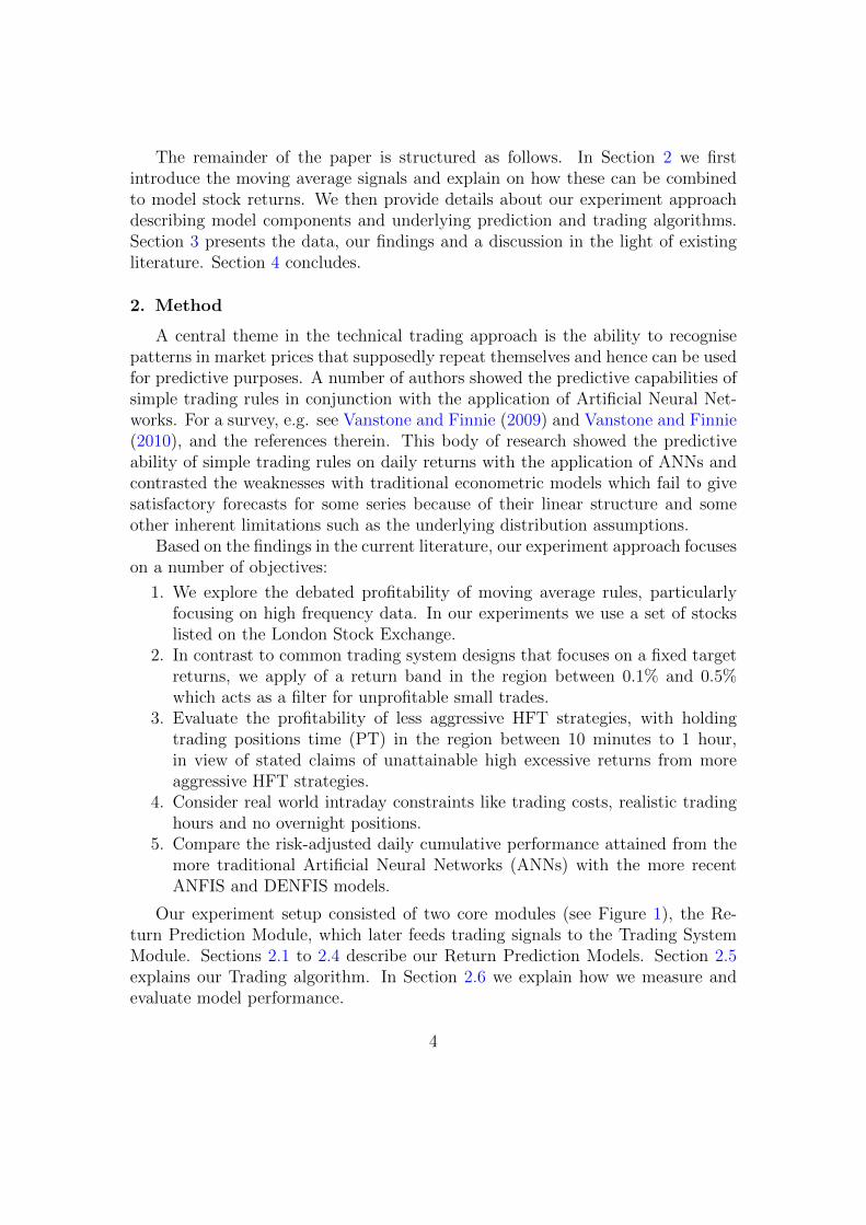
The remainder of the paper is structured as follows. In Section 2 we firstintroduce the moving average signals and explain on how these can be combinedto model stock returns. We then provide details about our experiment approachdescribing model components and underlying prediction and trading algorithms.Section 3 presents the data, our findings and a discussion in the light of existingliterature. Section 4 concludes.
2. Method
A central theme in the technical trading approach is the ability to recognisepatterns in market prices that supposedly repeat themselves and hence can be usedfor predictive purposes. A number of authors showed the predictive capabilities ofsimple trading rules in conjunction with the application of Artificial Neural Net-works. For a survey, e.g. see Vanstone and Finnie (2009) and Vanstone and Finnie(2010), and the references therein. This body of research showed the predictiveability of simple trading rules on daily returns with the application of ANNs andcontrasted the weaknesses with traditional econometric models which fail to givesatisfactory forecasts for some series because of their linear structure and someother inherent limitations such as the underlying distribution assumptions.
Based on the findings in the current literature, our experiment approach focuseson a number of objectives:
1. We explore the debated profitability of moving average rules, particularlyfocusing on high frequency data. In our experiments we use a set of stockslisted on the London Stock Exchange.
2. In contrast to common trading system designs that focuses on a fixed targetreturns, we apply of a return band in the region between 0.1% and 0.5%which acts as a filter for unprofitable small trades.
3. Evaluate the profitability of less aggressive HFT strategies, with holdingtrading positions time (PT) in the region between 10 minutes to 1 hour,in view of stated claims of unattainable high excessive returns from moreaggressive HFT strategies.
4. Consider real world intraday constraints like trading costs, realistic tradinghours and no overnight positions.
5. Compare the risk-adjusted daily cumulative performance attained from themore traditional Artificial Neural Networks (ANNs) with the more recentANFIS and DENFIS models.
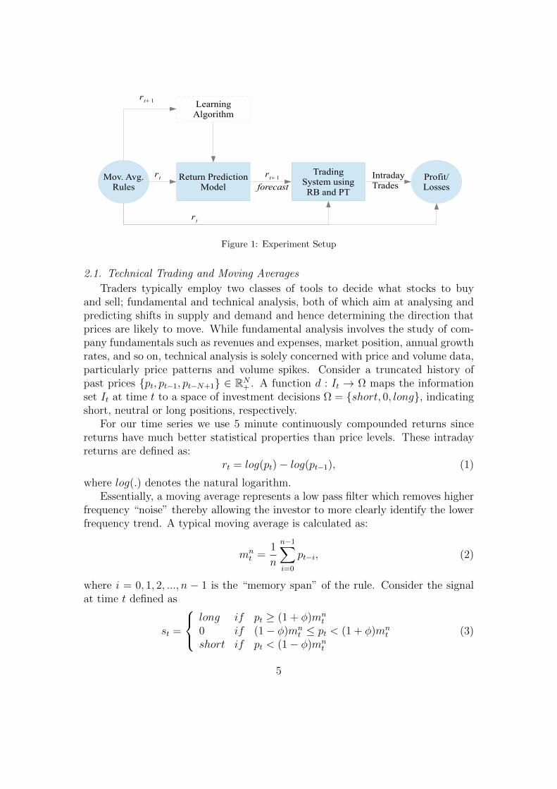
Our experiment setup consisted of two core modules (see Figure 1), the Re-turn Prediction Module, which later feeds trading signals to the Trading SystemModule. Sections 2.1 to 2.4 describe our Return Prediction Models. Section 2.5explains our Trading algorithm. In Section 2.6 we explain how we measure andevaluate model performance.
4
Return PredictionModel
TradingSystem usingRB and PT
Mov. Avg.Rules
LearningAlgorithm
Profit/Losses
IntradayTrades
r t+ 1
rt+ 1
forecast
r t
r t
Figure 1: Experiment Setup
2.1. Technical Trading and Moving Averages
Traders typically employ two classes of tools to decide what stocks to buyand sell; fundamental and technical analysis, both of which aim at analysing andpredicting shifts in supply and demand and hence determining the direction thatprices are likely to move. While fundamental analysis involves the study of com-pany fundamentals such as revenues and expenses, market position, annual growthrates, and so on, technical analysis is solely concerned with price and volume data,particularly price patterns and volume spikes. Consider a truncated history ofpast prices pt, pt−1, pt−N+1 ∈ RN
+ . A function d : It → Ω maps the informationset It at time t to a space of investment decisions Ω = short, 0, long, indicatingshort, neutral or long positions, respectively.
For our time series we use 5 minute continuously compounded returns sincereturns have much better statistical properties than price levels. These intradayreturns are defined as:
rt = log(pt)− log(pt−1), (1)
where log(.) denotes the natural logarithm.Essentially, a moving average represents a low pass filter which removes higher
frequency “noise” thereby allowing the investor to more clearly identify the lowerfrequency trend. A typical moving average is calculated as:
mnt =
1
n
n−1∑i=0
pt−i, (2)
where i = 0, 1, 2, ..., n − 1 is the “memory span” of the rule. Consider the signalat time t defined as
st =
long if pt ≥ (1 + φ)mn
t
0 if (1− φ)mnt ≤ pt < (1 + φ)mn
t
short if pt < (1− φ)mnt
(3)
5
where φ is the bandwidth of the rule for whiplash reduction.Another popular variation of the rule is:
sn1,n2t =
(mn1
t −mn2t ) if |mn1
t −mn2t | > φ
0 else(4)
where n1 and n2 are the short and long moving averages, respectively.We investigate whether intraday high frequency returns can be successfully
predicted by making use of buy and sell signals as inputs and use this informationto build a profitable trading algorithm. In this setting the linear regression modelis
rt = α +
p∑i=1
βisn1,n2
t−i + εt, (5)
where the error term εt is an independent variable with mean 0 and variance σ2t .
Kearns et al. (2010) recently noted that when taking transaction costs into ac-count, aggressive HFT strategies considering holding periods between 10 millisec-onds and 10 seconds can have surprisingly modest profitability. For this reason inour experiment we investigate the effect of applying less aggressive HFT strate-gies. We slow down our trading by investigating (a) longer holding periods rangingfrom 10 minutes to 1 hour, and (b) the application of a return band ranging from0.1% to 0.5%. This approach is more versatile than compared to the commonapproaches in the literature that calibrate their trading systems only based onan arbitrary target return. Brabazon and O’Neill (2006) showed that similar useof extended close in intraday trading scenarios can perform better than standardStop-Loss, Take-Profit and Buy-and-Hold strategies.
We first identify a model that predicts the next five-minute stock return bytaking a series of moving average signals as input variables. The three movingaverage rules utilised are (n1, n2) = [(1,5), (5,10), (10,15)], where n1 and n2 arein 5 minute time bars. In line with eq. (5), by combining these rules the linearspecification of the return prediction model is
rt = α + βis1,5t−i + βis
5,10t−i + βis
10,15t−i + εt, (6)
wheresn1,n2t = mn1
t −mn2t . (7)
In the following, we describe how the ANFIS, DENFIS and feed-forward net-work (FFN) models are adapted for our experiments.
2.2. ANFIS Model
Neuro-Fuzzy techniques synergise ANNs with Fuzzy Logic techniques by com-bining the human-like reasoning style of fuzzy systems with the learning and con-nectionist structure of neural networks. Algorithms for acquisition or tuning of
6
fuzzy models from data typically focus on one or all the following aspects (i) ruleconsequent parameter optimisation, (ii) membership function parameter optimi-sation and (iii) rule induction. The tested systems will be taking input from anumber of moving average rules and predict the stock return.
A popular technique is the Adaptive Neuro-Fuzzy inference system (ANFIS)suggested by Jang (1993). ANFIS presents a Takagi-Sugeno (TS) model in adifferent architecture that albeit the mathematical underpinnings are similar thestructure is formulated to permit ANN learning techniques. Following from thestandard ANFIS model and eq. (5), we apply the ANFIS architecture layers, de-noting the output of the i-th node in layer l as Ol,i, as follows:
Layer 1 The output of each node O1,i is the membership grade for the movingaverage signals s1,5t−1, s
5,10t−1 , s10,15t−1 . Different types and number of input
membership functions, and corresponding premise parameters, are tested inour model calibration process (see Table 1).
Layer 2 Every node in this layer is fixed. In this layer the t-norm is used to“AND” the membership grades, for example the product:
O2,i = wi = µAi(s1,5t−1)µBi
(s5,10t−1 )µCi(s10,15t−1 ). (8)
Layer 3 This layer contains fixed nodes which calculate the normalised firingstrengths of the rules:
O3,i = wi =wi
w1 + w2 + w3
. (9)
Layer 4 The nodes in this layer are adaptive and perform the consequent of therules:
O4,i = wifi = wi(αis1,5t−1 + βis
5,10t−1 + γis
10,15t−1 + δi). (10)
where wi is the normalised firing strength from the previous layer and fi isa linear function of the moving average signals with consequent parametersαi, βi, γi, δi.
Layer 5 This layer consists of a single node that computes the overall output Thenodes in this layer are adaptive and perform the consequent of the rules:
O5,i = rt =∑i
wifi =
∑wifi∑iwi
. (11)
7
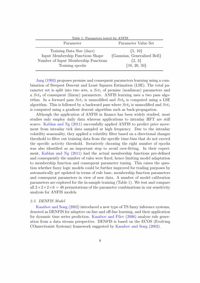
Table 1: Parameters tested for ANFIS
Parameter Parameter Value Set
Training Data Size (days) 5, 10Input Membership Functions Shape Gaussian, Generalised Bell
Number of Input Membership Functions 2, 3Training epochs 10, 20, 50
Jang (1993) proposes premise and consequent parameters learning using a com-bination of Steepest Descent and Least Squares Estimation (LSE). The total pa-rameter set is split into two sets, a Set1 of premise (nonlinear) parameters anda Set2 of consequent (linear) parameters. ANFIS learning uses a two pass algo-rithm. In a forward pass Set1 is unmodified and Set2 is computed using a LSEalgorithm. This is followed by a backward pass where Set2 is unmodified and Set1is computed using a gradient descent algorithm such as back-propagation.
Although the application of ANFIS in finance has been widely studied, moststudies only employ daily data whereas applications to intraday HFT are stillscarce. Kablan and Ng (2011) successfully applied ANFIS to predict price move-ment from intraday tick data sampled at high frequency. Due to the intradayvolatility seasonality, they applied a volatility filter based on a directional changesthreshold to filter out training data from the specific time-bins that do not exceedthe specific activity threshold. Iteratively choosing the right number of epochswas also identified as an important step to avoid over-fitting. In their experi-ment, Kablan and Ng (2011) had the actual membership functions pre-definedand consequently the number of rules were fixed, hence limiting model adaptationto membership function and consequent parameter tuning. This raises the ques-tion whether fuzzy logic models could be further improved for trading purposes byautomatically get updated in terms of rule base, membership function parametersand consequent parameters in view of new data. A number of model calibrationparameters are explored for the in-sample training (Table 1). We test and compareall 2×2×2×6 = 48 permutations of the parameter combinations in our sensitivityanalysis for ANFIS models.
2.3. DENFIS Model
Kasabov and Song (2002) introduced a new type of TS fuzzy inference systems,denoted as DENFIS for adaptive on-line and off-line learning, and their applicationfor dynamic time series prediction. Kasabov and Filev (2006) analyse rule gener-ation from a data stream perspective. DENFIS is based on the ECOS (EvolvingCOnnectionist Systems) framework suggested by Kasabov and Song (2002).
8
In our study, this distance is calculated by using the normalised Euclideandistance of a new sample to the cluster centres:
disti = ||Si − Cci||, (12)
where Si is the current example consisting of a moving average vector [s1,5t−1, s5,10t−1 ,
s10,15t−1 ] and Cci is the centre of cluster i. A threshold value Dthr is defined thatlimits the cluster size. When each data sample arrives, the steps below are carriedout (see also Kasabov and Song, 2002):
1. At the initial step of ECM, the first input data sample is considered as thefirst cluster with the data itself as the first cluster centre and cluster centreset to zero.
2. As a new data sample arrives, the distance dist between the samples and allother existing cluster centres are determined.
3. The cluster with minimum distance distmin is selected. If distmin is less thanthe radius then the sample is associated to the cluster and no updates arerequired.
4. For every existing cluster the respective dist is added to the radius (let thisvalue be range). The cluster with minimum range is selected. If range isless than 2 × Dthr then the sample belongs to the cluster, the radius ofthis cluster is updated to (range/2) and the cluster centre is updated bypositioning it in the line joining the data sample and the cluster centre sothat now the distance between the new centre and the sample is equal to thenew radius value.
5. If range is greater than 2 × Dthr then a new cluster is created as in step1. Each new cluster generates a new rule and evolves the structure of thesystem. As new data samples arrive new rules can be created and existingrules can be updated incrementally.
The inference engine in DENFIS is composed of m fuzzy rules indicated asfollows:
IF (s1,5t−1 is Ri,1) AND (s5,10t−1 is Ri,2) AND (s10,15t−1 is Ri,3)
THEN rt is fi(s1,5t−1, s
5,10t−1 , s
10,15t−1 ),
where i=1,2,...,m and j = 1, 2, 3; (sn1,n2
t−1 is Ri,j) are m× 3 fuzzy propositions as mantecedents for m fuzzy rules; and Ri,j are fuzzy sets defined by their fuzzy mem-bership functions µRi,j
: sn1,n2
t−1 → [0, 1]. In the consequent part, linear functions fi,where i=1,2...,m are employed. In DENFIS, all fuzzy membership functions aretriangular type functions defined by three parameters:
µ(sn1,n2
t−1 , a, b, c) = max
(min
(sn1,n2
t−1 − ab− a
,c− sn1,n2
t−1
c− b
), 0
), (13)
9
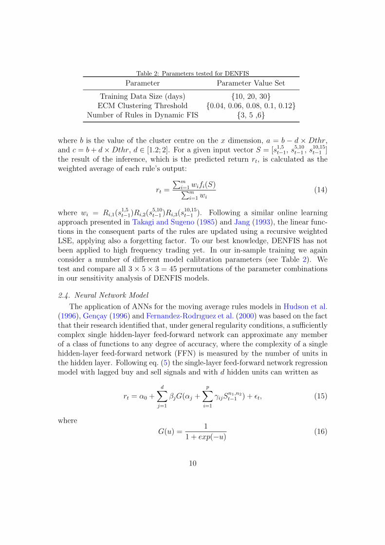
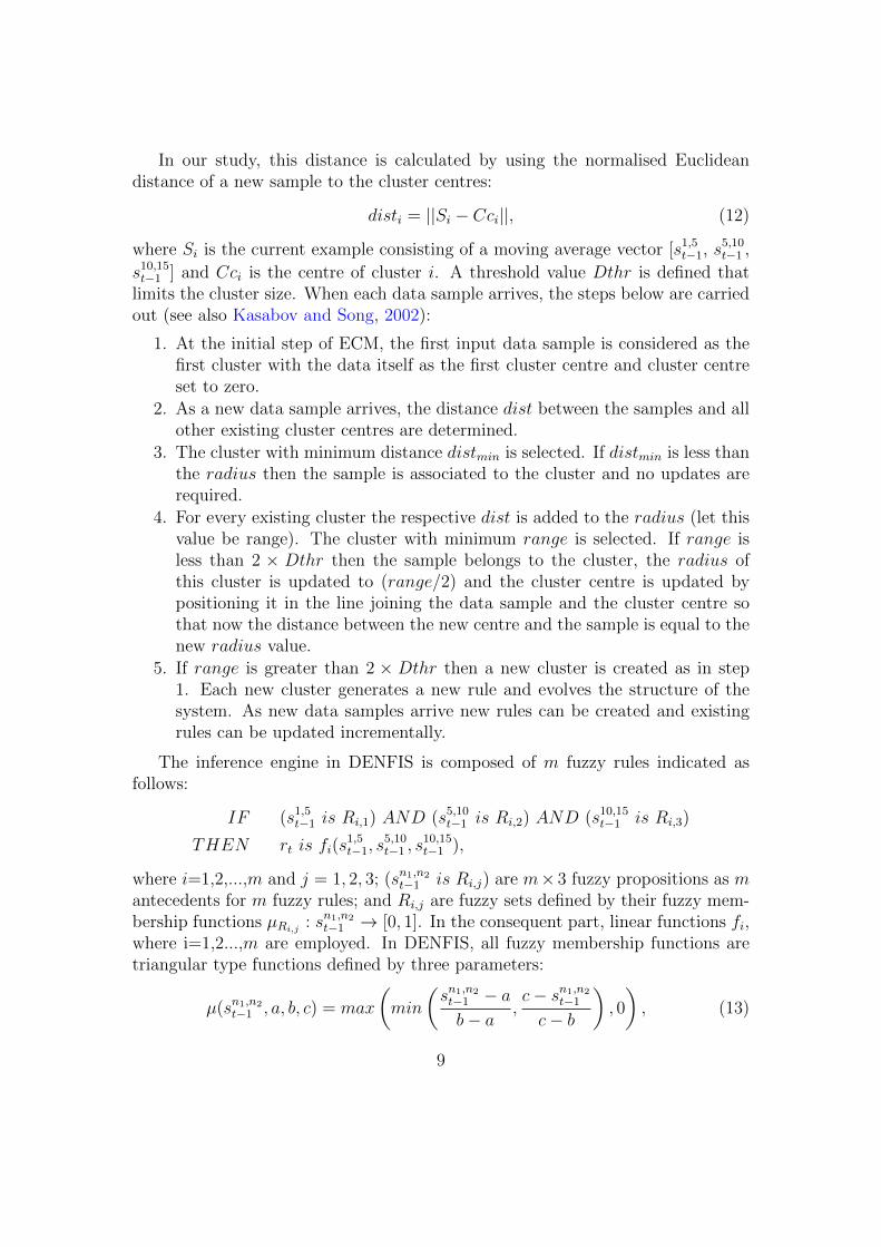
Table 2: Parameters tested for DENFIS
Parameter Parameter Value Set
Training Data Size (days) 10, 20, 30ECM Clustering Threshold 0.04, 0.06, 0.08, 0.1, 0.12
Number of Rules in Dynamic FIS 3, 5 ,6
where b is the value of the cluster centre on the x dimension, a = b − d × Dthr,and c = b+ d×Dthr, d ∈ [1.2; 2]. For a given input vector S = [s1,5t−1, s
5,10t−1 , s10,15t−1 ]
the result of the inference, which is the predicted return rt, is calculated as theweighted average of each rule’s output:
rt =
∑mi=1wifi(S)∑m
i=1wi
(14)
where wi = Ri,1(s1,5t−1)Ri,2(s
5,10t−1 )Ri,3(s
10,15t−1 ). Following a similar online learning
approach presented in Takagi and Sugeno (1985) and Jang (1993), the linear func-tions in the consequent parts of the rules are updated using a recursive weightedLSE, applying also a forgetting factor. To our best knowledge, DENFIS has notbeen applied to high frequency trading yet. In our in-sample training we againconsider a number of different model calibration parameters (see Table 2). Wetest and compare all 3× 5× 3 = 45 permutations of the parameter combinationsin our sensitivity analysis of DENFIS models.
2.4. Neural Network Model
The application of ANNs for the moving average rules models in Hudson et al.(1996), Gencay (1996) and Fernandez-Rodrıguez et al. (2000) was based on the factthat their research identified that, under general regularity conditions, a sufficientlycomplex single hidden-layer feed-forward network can approximate any memberof a class of functions to any degree of accuracy, where the complexity of a singlehidden-layer feed-forward network (FFN) is measured by the number of units inthe hidden layer. Following eq. (5) the single-layer feed-forward network regressionmodel with lagged buy and sell signals and with d hidden units can written as
rt = α0 +d∑
j=1
βjG(αj +
p∑i=1
γijSn1,n2
t−1 ) + εt, (15)
where
G(u) =1
1 + exp(−u)(16)
10
Table 3: Parameters tested for FFN
Parameter Parameter Value Set
Training Data Size (days) 5, 10Number of Hidden Units 5, 10, 20
Max Training epochs 1000
is the activation function in our application. For our model identification a numberof model parameters are considered during the in-sample training (see Table 3).We test and compare all 2×3×1 = 6 permutations of the parameter combinationsin our sensitivity analysis of FFN models.
2.5. Trading Algorithm
The second module of our trading system (see Figure 1) consists of a tradingand money management algorithm that takes the 5 minute return predictions fromthe first module and performs trades based on specific rules (see also Tan et al.,2011; Vanstone and Finnie, 2009, 2010). An HFT algorithm has to automate anumber of decisions: (i) what to buy or sell (markets), (ii) how much to buy orsell (position sizing), (iii) when to buy or sell (entries), (iv) when to go out of alosing position (stops), (v) when to go out of a winning position (exits), and (vi)how to buy or sell (tactics). Our focus in this paper is particularly on decisions(iii) to (v).
The objective of our trading algorithm is to generate buy, sell or do-nothingsignals. For buy or sell signals the predicted return value has to be greater (smaller)than the upper (lower) limits of a specific return band otherwise the trade signal isset to do-nothing. This was introduced in order to filter whiplash effects when theshort and long moving averages are close and also limit the number of small tradeswhich even if profitable would result in a loss due to transaction costs. In contrastto the common approach in the literature focusing on a single target return, weconsider different return bands between 0.1% and 0.5% for each stock to searchfor the optimal return during the in-sample period of 100 trading days. Based onthe selected band size, the position taken at time t is:
positiont =
long : rt > returnbandshort : rt < returnband
0 : otherwise.(17)
In our experiments we train the models on a daily rolling window basis, henceadapting the model on the most recent market scenarios of 100 in-sample days,followed by another 100 out-of-sample days, totalling 10,200 5 minute prices for
11
Algorithm 1 Pseudo code for position time
if position duration > PT thenif position direction = position directionpred then
position state← keep openposition open time← current time
elseposition state← close
end ifelse
position duration← current time− position open timeend if
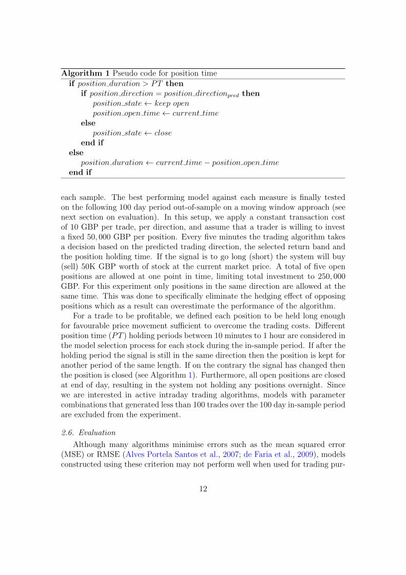
each sample. The best performing model against each measure is finally testedon the following 100 day period out-of-sample on a moving window approach (seenext section on evaluation). In this setup, we apply a constant transaction costof 10 GBP per trade, per direction, and assume that a trader is willing to investa fixed 50, 000 GBP per position. Every five minutes the trading algorithm takesa decision based on the predicted trading direction, the selected return band andthe position holding time. If the signal is to go long (short) the system will buy(sell) 50K GBP worth of stock at the current market price. A total of five openpositions are allowed at one point in time, limiting total investment to 250, 000GBP. For this experiment only positions in the same direction are allowed at thesame time. This was done to specifically eliminate the hedging effect of opposingpositions which as a result can overestimate the performance of the algorithm.
For a trade to be profitable, we defined each position to be held long enoughfor favourable price movement sufficient to overcome the trading costs. Differentposition time (PT ) holding periods between 10 minutes to 1 hour are considered inthe model selection process for each stock during the in-sample period. If after theholding period the signal is still in the same direction then the position is kept foranother period of the same length. If on the contrary the signal has changed thenthe position is closed (see Algorithm 1). Furthermore, all open positions are closedat end of day, resulting in the system not holding any positions overnight. Sincewe are interested in active intraday trading algorithms, models with parametercombinations that generated less than 100 trades over the 100 day in-sample periodare excluded from the experiment.
2.6. Evaluation
Although many algorithms minimise errors such as the mean squared error(MSE) or RMSE (Alves Portela Santos et al., 2007; de Faria et al., 2009), modelsconstructed using these criterion may not perform well when used for trading pur-
12
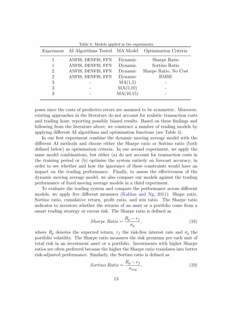
Table 4: Models applied in the experiments
Experiment AI Algorithms Tested MA Model Optimisation Criteria
1 ANFIS, DENFIS, FFN Dynamic Sharpe Ratio1 ANFIS, DENFIS, FFN Dynamic Sortino Ratio2 ANFIS, DENFIS, FFN Dynamic Sharpe Ratio, No Cost2 ANFIS, DENFIS, FFN Dynamic RMSE3 - MA(1,5) -3 - MA(5,10) -3 - MA(10,15) -
poses since the costs of predictive errors are assumed to be symmetric. Moreover,existing approaches in the literature do not account for realistic transaction costsand trading hour, reporting possibly biased results. Based on these findings andfollowing from the literature above, we construct a number of trading models byapplying different AI algorithms and optimisation functions (see Table 4).
In our first experiment combine the dynamic moving average model with thedifferent AI methods and choose either the Sharpe ratio or Sortino ratio (bothdefined below) as optimisation criteria. In our second experiment, we apply thesame model combinations, but either (a) do not account for transaction costs inthe training period or (b) optimise the system entirely on forecast accuracy, inorder to see whether and how the ignorance of these constraints would have animpact on the trading performance. Finally, to assess the effectiveness of thedynamic moving average model, we also compare our models against the tradingperformance of fixed moving average models in a third experiment.
To evaluate the trading system and compare the performance across differentmodels, we apply five different measures (Kablan and Ng, 2011): Shape ratio,Sortino ratio, cumulative return, profit ratio, and win ratio. The Sharpe ratioindicates to investors whether the returns of an asset or a portfolio come from asmart trading strategy or excess risk. The Sharpe ratio is defined as
Sharpe Ratio =Rp − rfσp
, (18)
where Rp denotes the expected return, rf the risk-free interest rate and σp theportfolio volatility. The Sharpe ratio measures the risk premium per each unit oftotal risk in an investment asset or a portfolio. Investments with higher Sharperatios are often preferred because the higher the Sharpe ratio translates into betterrisk-adjusted performance. Similarly, the Sortino ratio is defined as
Sortino Ratio =Rp − rfσneg
, (19)
13
where σneg denotes the standard deviation of only negative asset returns. Thus,the Sortino ratio measures the risk premium per each unit of downside risk inan investment asset or a portfolio. The cumulative return indicates the overallprobability of the strategy since the first trade, similar to a buy-and-hold scenario.
It should also be noted that the choice of performance function determines howoften the system trades and what percentage of its trades are winning trades. Theprofit ratio indicates a system’s ability to generate profits over losses and is definedas
Profit Ratio =Total Gain/Number of winning trades
Total Loss/Number of losing trades(20)
The win ratio is the ratio between the number of winning trades and losing tradesand is defined as
Win Ratio =Total Number of winning trades
Total Number of losing trades(21)
It has to be noted that albeit the profit and win ratios give an indication of thesystem’s performance, however it does not take into consideration the underlyingrisk (a single loss of $100 cannot compensate 99 winning trades of $1). Theseratios are however selected to validate whether the models showing higher riskreflect higher returns or higher number of wins.
Albeit many researchers claim the results of their algorithmic trading modelsby analysing a set of performance measures at a single point in time, covering aspecified number of days in the out-of-sample period, our interest is to validateour models by looking at cumulated risk-return measures on a day by day basis.This method provides a clearer analysis of the models’ behaviour and performancepattern over time. A range of model parameter combinations are tested resultingin∏n
i=1 pseti different models per algorithm, where n is the number of algorithmparameters and pseti is the number of unique discrete values tested for each pa-rameter i. In order to select a model with good generalisation capabilities eachmodel was trained and tested over a 100 day period using a rolling window ap-proach. Each model was trained on dayn−1 − dayn−1−s days of 5 minute returnsand tested on dayn 5 minute returns, where n = 1, 2, . . . , 100 is a day index ands is the training size in days used for the specific model. This requires that thefirst s days from the data set are reserved for training.
Furthermore, we also conduct a sensitivity analysis of the different modelsin order to investigate the uncertainty in the predicted output (see also Resta,2009). By inspecting our 100 day-by-day trading results and analyse these acrossthe regions in the space of input factors, we can utilise a heat map approachto identify areas which maximised the Sharpe ratio criterion (for illustration, seeFigures 2-4 in the next section). In particular, we are interested to see how themodels behave across different levels of position time and return band parameters.
14
3. Empirical Data and Analysis
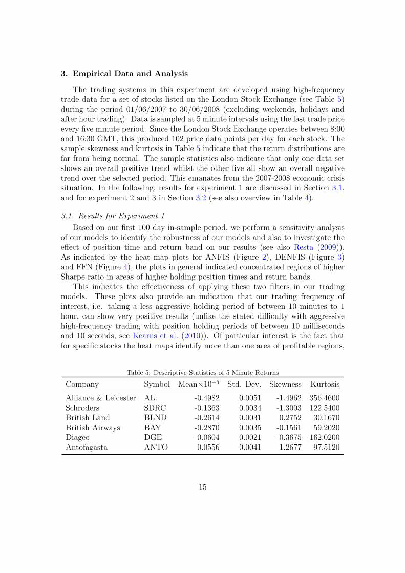
The trading systems in this experiment are developed using high-frequencytrade data for a set of stocks listed on the London Stock Exchange (see Table 5)during the period 01/06/2007 to 30/06/2008 (excluding weekends, holidays andafter hour trading). Data is sampled at 5 minute intervals using the last trade priceevery five minute period. Since the London Stock Exchange operates between 8:00and 16:30 GMT, this produced 102 price data points per day for each stock. Thesample skewness and kurtosis in Table 5 indicate that the return distributions arefar from being normal. The sample statistics also indicate that only one data setshows an overall positive trend whilst the other five all show an overall negativetrend over the selected period. This emanates from the 2007-2008 economic crisissituation. In the following, results for experiment 1 are discussed in Section 3.1,and for experiment 2 and 3 in Section 3.2 (see also overview in Table 4).
3.1. Results for Experiment 1
Based on our first 100 day in-sample period, we perform a sensitivity analysisof our models to identify the robustness of our models and also to investigate theeffect of position time and return band on our results (see also Resta (2009)).As indicated by the heat map plots for ANFIS (Figure 2), DENFIS (Figure 3)and FFN (Figure 4), the plots in general indicated concentrated regions of higherSharpe ratio in areas of higher holding position times and return bands.
This indicates the effectiveness of applying these two filters in our tradingmodels. These plots also provide an indication that our trading frequency ofinterest, i.e. taking a less aggressive holding period of between 10 minutes to 1hour, can show very positive results (unlike the stated difficulty with aggressivehigh-frequency trading with position holding periods of between 10 millisecondsand 10 seconds, see Kearns et al. (2010)). Of particular interest is the fact thatfor specific stocks the heat maps identify more than one area of profitable regions,
Table 5: Descriptive Statistics of 5 Minute Returns
Company Symbol Mean×10−5 Std. Dev. Skewness Kurtosis
Alliance & Leicester AL. -0.4982 0.0051 -1.4962 356.4600Schroders SDRC -0.1363 0.0034 -1.3003 122.5400British Land BLND -0.2614 0.0031 0.2752 30.1670British Airways BAY -0.2870 0.0035 -0.1561 59.2020Diageo DGE -0.0604 0.0021 -0.3675 162.0200Antofagasta ANTO 0.0556 0.0041 1.2677 97.5120
15
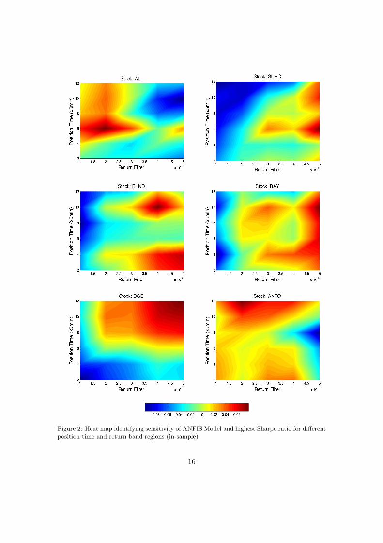
Figure 2: Heat map identifying sensitivity of ANFIS Model and highest Sharpe ratio for differentposition time and return band regions (in-sample)
16
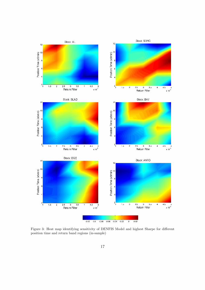
Figure 3: Heat map identifying sensitivity of DENFIS Model and highest Sharpe for differentposition time and return band regions (in-sample)
17
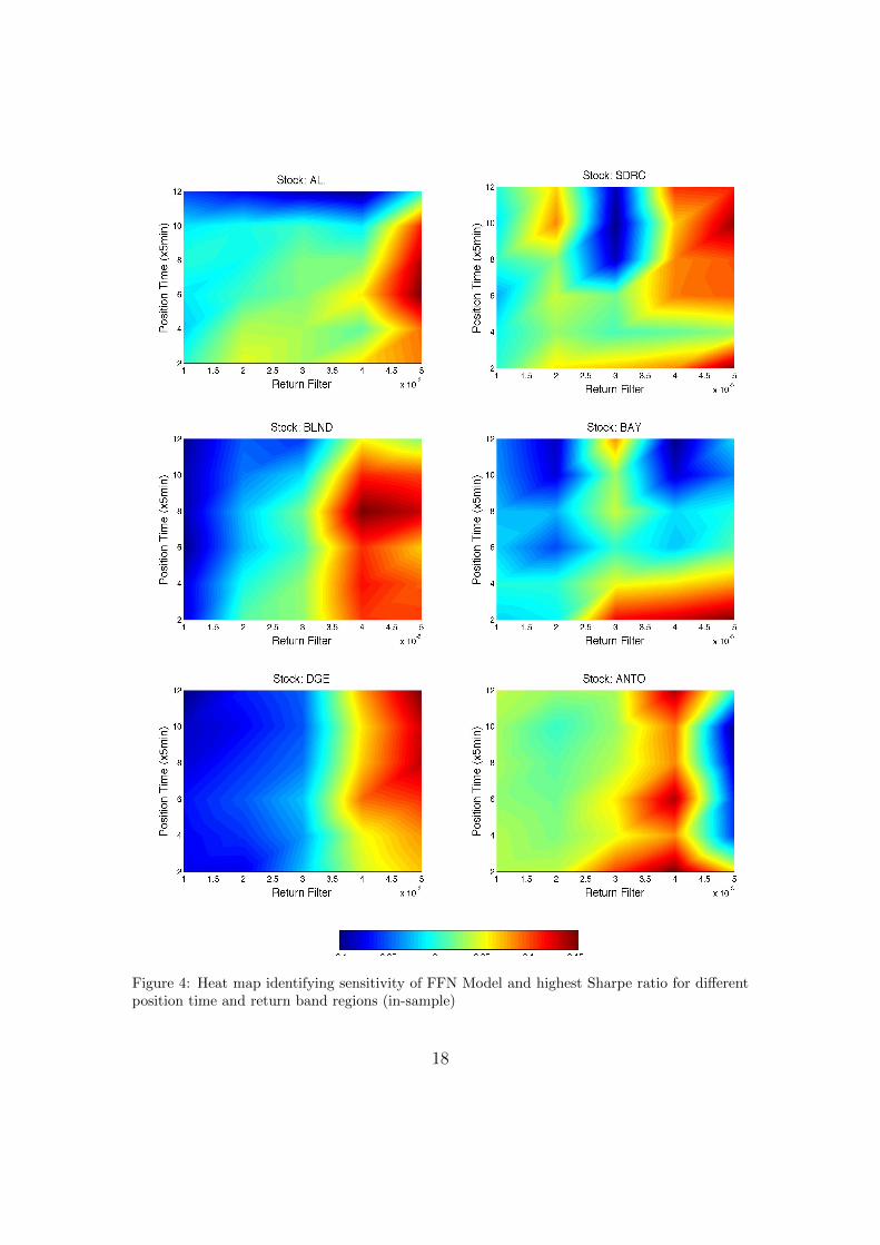
Figure 4: Heat map identifying sensitivity of FFN Model and highest Sharpe ratio for differentposition time and return band regions (in-sample)
18
20 30 40 50 60 70 80 90 100−0.6
−0.5
−0.4
−0.3
−0.2
−0.1
0
0.1
0.2
0.3Stock: AL.
Days
Sh
arp
e R
atio
20 30 40 50 60 70 80 90 100−0.3
−0.2
−0.1
0
0.1
0.2
0.3
0.4
0.5Stock: SDRC
Days
Sh
arp
e R
atio
20 30 40 50 60 70 80 90 100−0.05
0
0.05
0.1
0.15
0.2
0.25
0.3
0.35
0.4Stock: BLND
Days
Sh
arp
e R
atio
20 30 40 50 60 70 80 90 1000.1
0.2
0.3
0.4
0.5
0.6Stock: BAY
Days
Sh
arp
e R
atio
20 30 40 50 60 70 80 90 100−0.4
−0.3
−0.2
−0.1
0
0.1
0.2
0.3Stock: DGE
Days
Sh
arp
e R
atio
20 30 40 50 60 70 80 90 100−0.1
−0.08
−0.06
−0.04
−0.02
0
0.02
0.04Stock: ANTO
Days
Sh
arp
e R
atio
ANFIS DENFIS FFN
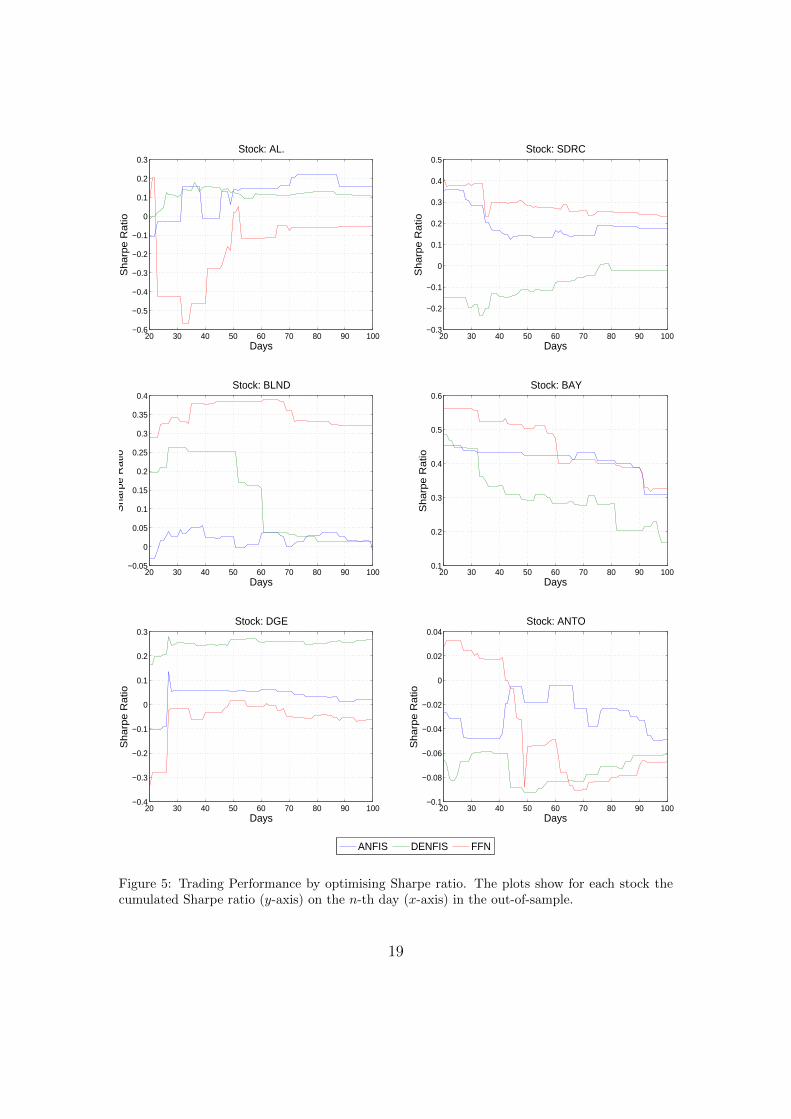
Figure 5: Trading Performance by optimising Sharpe ratio. The plots show for each stock thecumulated Sharpe ratio (y-axis) on the n-th day (x-axis) in the out-of-sample.
19
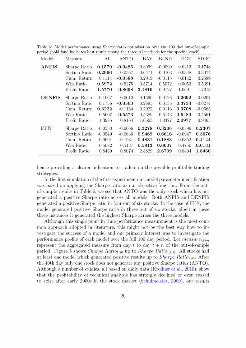
Table 6: Model performance using Sharpe ratio optimisation over the 100 day out-of-sampleperiod (bold fond indicates best result among the three AI methods for the specific stock)
Model Measure AL. ANTO BAY BLND DGE SDRC
ANFIS Sharpe Ratio 0.1579 -0.0485 0.3099 -0.0090 0.0213 0.1748Sortino Ratio 0.2966 -0.0567 0.6471 -0.0103 0.0348 0.3074Cum. Return 0.1114 -0.0588 0.2919 -0.0115 0.0142 0.2589Win Ratio 0.5972 0.5275 0.5714 0.5072 0.5053 0.5391Profit Ratio 1.5770 0.8698 3.1816 0.9727 1.0691 1.7313
DENFIS Sharpe Ratio 0.1067 -0.0610 0.1690 0.0126 0.2692 -0.0207Sortino Ratio 0.1756 -0.0563 0.2895 0.0135 0.3734 -0.0274Cum. Return 0.3222 -0.1154 0.2922 0.0113 0.3708 -0.0565Win Ratio 0.5607 0.5573 0.5389 0.5143 0.6480 0.5561Profit Ratio 1.3985 0.8164 1.6663 1.0377 2.0977 0.9465
FFN Sharpe Ratio -0.0553 -0.0666 0.3278 0.3206 -0.0599 0.2307Sortino Ratio -0.0549 -0.0636 0.9469 0.6616 -0.0947 0.3676Cum. Return -0.0691 -0.1931 0.4831 0.1883 -0.0352 0.4144Win Ratio 0.5082 0.5437 0.5913 0.6607 0.4750 0.6131Profit Ratio 0.8459 0.8074 2.8829 2.6709 0.8494 1.8460
hence providing a clearer indication to traders on the possible profitable tradingstrategies.
In the first simulation of the first experiment our model parameter identificationwas based on applying the Sharpe ratio as our objective function. From the out-of-sample results in Table 6, we see that ANTO was the only stock which has notgenerated a positive Sharpe ratio across all models. Both ANFIS and DENFISgenerated a positive Sharpe ratio in four out of six stocks. In the case of FFN, themodel generated positive Sharpe ratio in three out of six stocks, albeit in thesethree instances it generated the highest Sharpe across the three models.
Although this single point in time performance measurement is the most com-mon approach adopted in literature, this might not be the best way how to in-vestigate the success of a model and our primary interest was to investigate theperformance profile of each model over the full 100 day period. Let measuret,t+n
represent the aggregated measure from day t to day t + n of the out-of-sampleperiod. Figure 5 shows Sharpe Ratio1,20 up to Sharpe Ratio1,100. All stocks hadat least one model which generated positive results up to Sharpe Ratio1,40. Afterthe 40th day only one stock does not generate any positive Sharpe ratios (ANTO).Although a number of studies, all based on daily data (Krollner et al., 2010), showthat the profitability of technical analysis has strongly declined or even ceasedto exist after early 2000s in the stock market (Schulmeister, 2009), our results
20
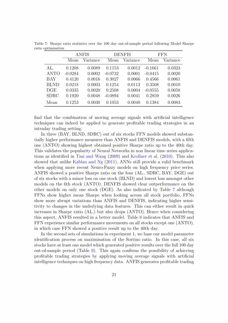
Table 7: Sharpe ratio statistics over the 100 day out-of-sample period following Model Sharperatio optimisation
ANFIS DENFIS FFNMean Variance Mean Variance Mean Variance
AL. 0.1208 0.0089 0.1153 0.0012 -0.1661 0.0323ANTO -0.0284 0.0002 -0.0732 0.0001 -0.0415 0.0020BAY 0.4120 0.0016 0.3027 0.0066 0.4566 0.0061BLND 0.0218 0.0003 0.1254 0.0113 0.3508 0.0010DGE 0.0335 0.0020 0.2508 0.0004 -0.0555 0.0058SDRC 0.1920 0.0048 -0.0894 0.0041 0.2859 0.0026
Mean 0.1253 0.0030 0.1053 0.0040 0.1384 0.0083
find that the combination of moving average signals with artificial intelligencetechniques can indeed be applied to generate profitable trading strategies in anintraday trading setting.
In three (BAY, BLND, SDRC) out of six stocks FFN models showed substan-tially higher performance measures than ANFIS and DENFIS models, with a fifthone (ANTO) showing highest obtained positive Sharpe ratio up to the 40th day.This validates the popularity of Neural Networks in non linear time series applica-tions as identified in Tsai and Wang (2009) and Krollner et al. (2010). This alsoshowed that unlike Kablan and Ng (2011), ANNs still provide a valid benchmarkwhen applying more recent Neuro-Fuzzy models on high frequency price series.ANFIS showed a positive Sharpe ratio on the four (AL., SDRC, BAY, DGE) outof six stocks with a minor loss on one stock (BLND) and lowest loss amongst othermodels on the 6th stock (ANTO). DENFIS showed clear outperformance on theother models on only one stock (DGE). As also indicated by Table 7 althoughFFNs show higher mean Sharpe when looking across all stock portfolio, FFNsshow more abrupt variations than ANFIS and DENFIS, indicating higher sensi-tivity to changes in the underlying data features. This can either result in quickincreases in Sharpe ratio (AL.) but also drops (ANTO). Hence when consideringthis aspect, ANFIS resulted in a better model. Table 8 indicates that ANFIS andFFN experience similar performance movements on all stocks except one (ANTO),in which case FFN showed a positive result up to the 40th day.
In the second sets of simulations in experiment 1, we base our model parameteridentification process on maximisation of the Sortino ratio. In this case, all sixstocks have at least one model which generated positive results over the full 100 dayout-of-sample period (Table 9). This again confirms the possibility of achievingprofitable trading strategies by applying moving average signals with artificialintelligence techniques on high frequency data. ANFIS generates profitable trading
21
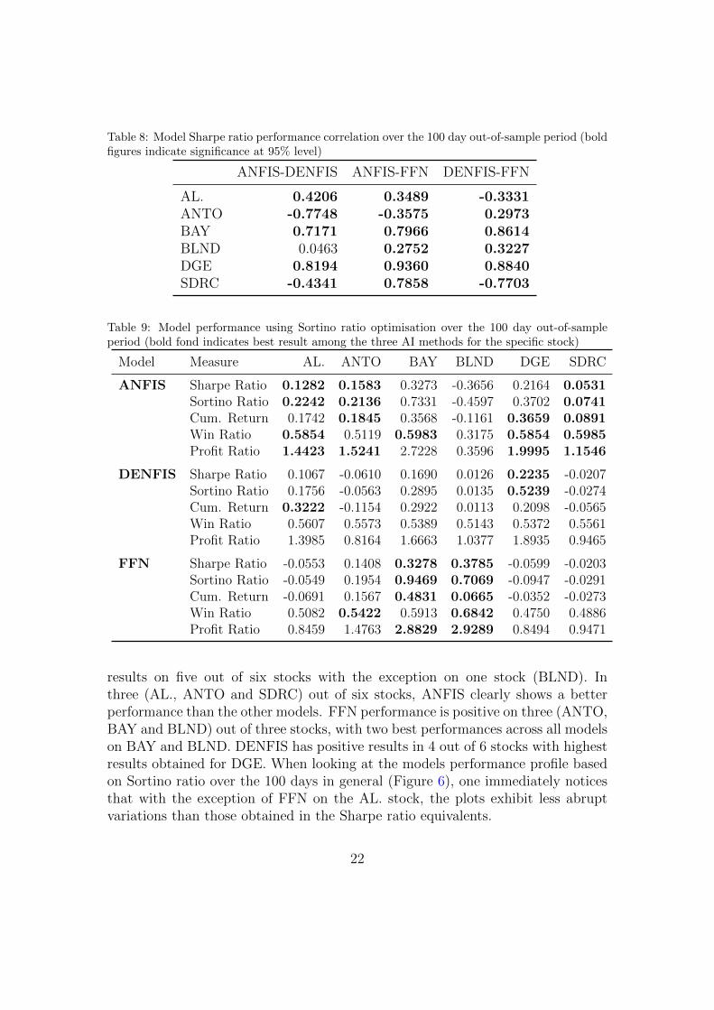
Table 8: Model Sharpe ratio performance correlation over the 100 day out-of-sample period (boldfigures indicate significance at 95% level)
ANFIS-DENFIS ANFIS-FFN DENFIS-FFN
AL. 0.4206 0.3489 -0.3331ANTO -0.7748 -0.3575 0.2973BAY 0.7171 0.7966 0.8614BLND 0.0463 0.2752 0.3227DGE 0.8194 0.9360 0.8840SDRC -0.4341 0.7858 -0.7703
Table 9: Model performance using Sortino ratio optimisation over the 100 day out-of-sampleperiod (bold fond indicates best result among the three AI methods for the specific stock)
Model Measure AL. ANTO BAY BLND DGE SDRC
ANFIS Sharpe Ratio 0.1282 0.1583 0.3273 -0.3656 0.2164 0.0531Sortino Ratio 0.2242 0.2136 0.7331 -0.4597 0.3702 0.0741Cum. Return 0.1742 0.1845 0.3568 -0.1161 0.3659 0.0891Win Ratio 0.5854 0.5119 0.5983 0.3175 0.5854 0.5985Profit Ratio 1.4423 1.5241 2.7228 0.3596 1.9995 1.1546
DENFIS Sharpe Ratio 0.1067 -0.0610 0.1690 0.0126 0.2235 -0.0207Sortino Ratio 0.1756 -0.0563 0.2895 0.0135 0.5239 -0.0274Cum. Return 0.3222 -0.1154 0.2922 0.0113 0.2098 -0.0565Win Ratio 0.5607 0.5573 0.5389 0.5143 0.5372 0.5561Profit Ratio 1.3985 0.8164 1.6663 1.0377 1.8935 0.9465
FFN Sharpe Ratio -0.0553 0.1408 0.3278 0.3785 -0.0599 -0.0203Sortino Ratio -0.0549 0.1954 0.9469 0.7069 -0.0947 -0.0291Cum. Return -0.0691 0.1567 0.4831 0.0665 -0.0352 -0.0273Win Ratio 0.5082 0.5422 0.5913 0.6842 0.4750 0.4886Profit Ratio 0.8459 1.4763 2.8829 2.9289 0.8494 0.9471
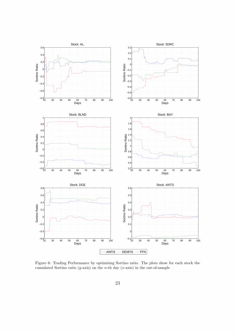
results on five out of six stocks with the exception on one stock (BLND). Inthree (AL., ANTO and SDRC) out of six stocks, ANFIS clearly shows a betterperformance than the other models. FFN performance is positive on three (ANTO,BAY and BLND) out of three stocks, with two best performances across all modelson BAY and BLND. DENFIS has positive results in 4 out of 6 stocks with highestresults obtained for DGE. When looking at the models performance profile basedon Sortino ratio over the 100 days in general (Figure 6), one immediately noticesthat with the exception of FFN on the AL. stock, the plots exhibit less abruptvariations than those obtained in the Sharpe ratio equivalents.
22
20 30 40 50 60 70 80 90 100−0.8
−0.6
−0.4
−0.2
0
0.2
0.4
0.6Stock: AL.
Days
So
rtin
o R
atio
20 30 40 50 60 70 80 90 100−0.6
−0.5
−0.4
−0.3
−0.2
−0.1
0
0.1
0.2
0.3Stock: SDRC
Days
So
rtin
o R
atio
20 30 40 50 60 70 80 90 100−0.6
−0.4
−0.2
0
0.2
0.4
0.6
0.8
1Stock: BLND
Days
So
rtin
o R
atio
20 30 40 50 60 70 80 90 1000.2
0.4
0.6
0.8
1
1.2
1.4
1.6
1.8
2Stock: BAY
Days
So
rtin
o R
atio
20 30 40 50 60 70 80 90 100−0.6
−0.4
−0.2
0
0.2
0.4
0.6
0.8Stock: DGE
Days
So
rtin
o R
atio
20 30 40 50 60 70 80 90 100−0.1
0
0.1
0.2
0.3
0.4
0.5
0.6Stock: ANTO
Days
So
rtin
o R
atio
ANFIS DENFIS FFN
Figure 6: Trading Performance by optimising Sortino ratio. The plots show for each stock thecumulated Sortino ratio (y-axis) on the n-th day (x-axis) in the out-of-sample
23
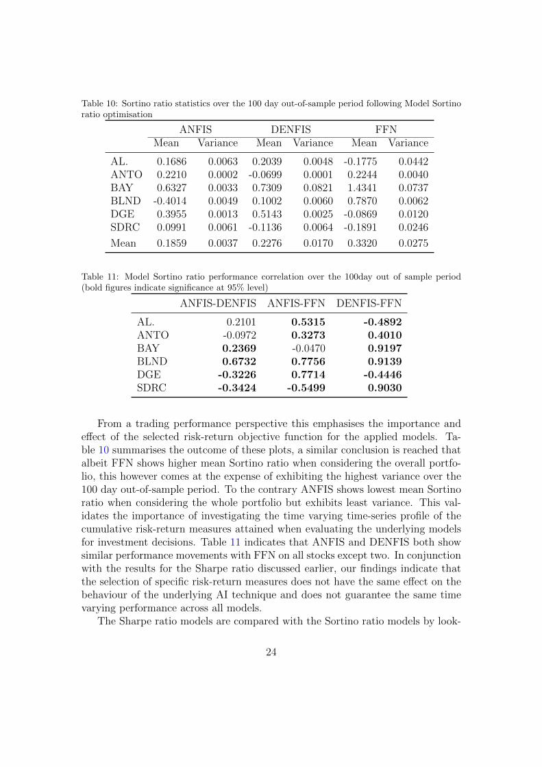
Table 10: Sortino ratio statistics over the 100 day out-of-sample period following Model Sortinoratio optimisation
ANFIS DENFIS FFNMean Variance Mean Variance Mean Variance
AL. 0.1686 0.0063 0.2039 0.0048 -0.1775 0.0442ANTO 0.2210 0.0002 -0.0699 0.0001 0.2244 0.0040BAY 0.6327 0.0033 0.7309 0.0821 1.4341 0.0737BLND -0.4014 0.0049 0.1002 0.0060 0.7870 0.0062DGE 0.3955 0.0013 0.5143 0.0025 -0.0869 0.0120SDRC 0.0991 0.0061 -0.1136 0.0064 -0.1891 0.0246
Mean 0.1859 0.0037 0.2276 0.0170 0.3320 0.0275
Table 11: Model Sortino ratio performance correlation over the 100day out of sample period(bold figures indicate significance at 95% level)
ANFIS-DENFIS ANFIS-FFN DENFIS-FFN
AL. 0.2101 0.5315 -0.4892ANTO -0.0972 0.3273 0.4010BAY 0.2369 -0.0470 0.9197BLND 0.6732 0.7756 0.9139DGE -0.3226 0.7714 -0.4446SDRC -0.3424 -0.5499 0.9030
From a trading performance perspective this emphasises the importance andeffect of the selected risk-return objective function for the applied models. Ta-ble 10 summarises the outcome of these plots, a similar conclusion is reached thatalbeit FFN shows higher mean Sortino ratio when considering the overall portfo-lio, this however comes at the expense of exhibiting the highest variance over the100 day out-of-sample period. To the contrary ANFIS shows lowest mean Sortinoratio when considering the whole portfolio but exhibits least variance. This val-idates the importance of investigating the time varying time-series profile of thecumulative risk-return measures attained when evaluating the underlying modelsfor investment decisions. Table 11 indicates that ANFIS and DENFIS both showsimilar performance movements with FFN on all stocks except two. In conjunctionwith the results for the Sharpe ratio discussed earlier, our findings indicate thatthe selection of specific risk-return measures does not have the same effect on thebehaviour of the underlying AI technique and does not guarantee the same timevarying performance across all models.
The Sharpe ratio models are compared with the Sortino ratio models by look-
24
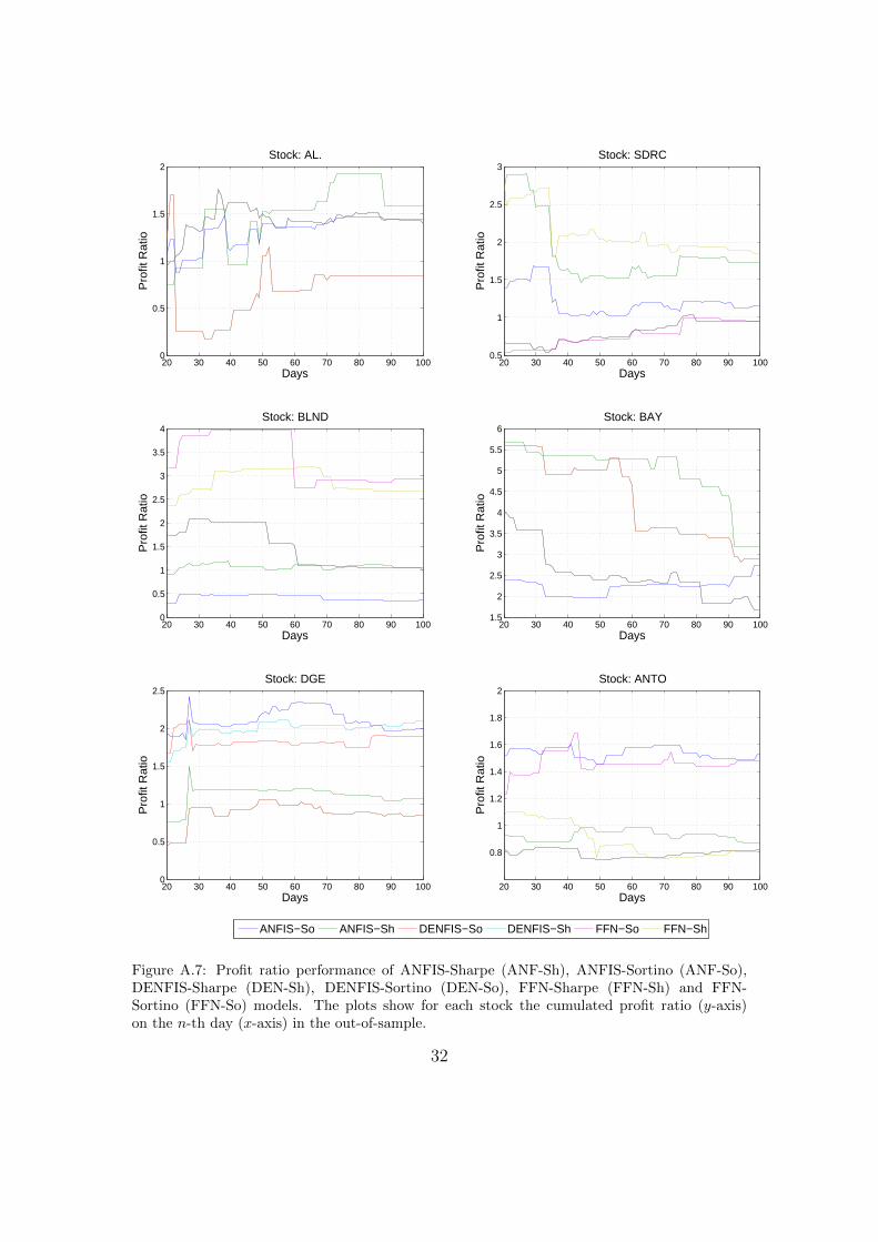
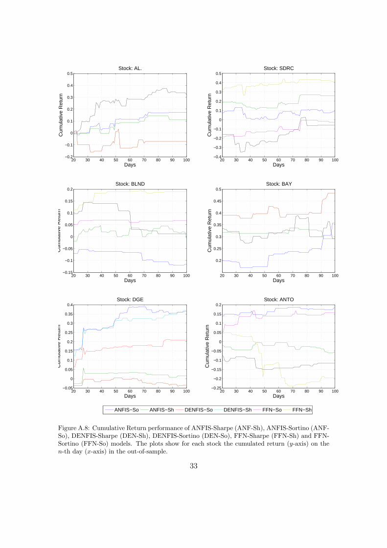
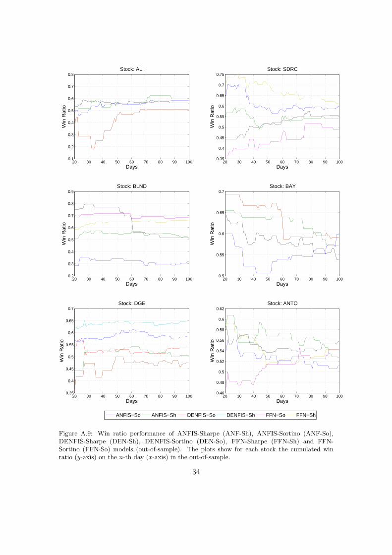
ing at their attained profit ratios (see Figure A.7). In general, the plots show atendency to group into two performance strata across the 100 day period, a closegroup competing on the higher side whilst another group giving similar perfor-mance on the lower side. With the exception of the last part of the DGE timeseries, a better performance for the rest of the stocks is attained by ANFIS orFFN models. For SDRC, BAY, DGE and ANTO the plots show that Sortinoand Sharpe ratio maximisation has a similar effect on ANFIS and FFN modelswhich result in obtaining a profit ratio time series in a higher or lower band fora specific stock. This distinction is less evident in DENFIS. In contrast to Schul-meister (2009) who demonstrated that aggressive HFT exhibit a surprisingly lowprofitability, our results show that the cumulative return (Figure A.8) and winratio (Figure A.9) from a number of models is considerably high. However, in linewith Brabazon and O’Neill (2006), a point worth noting is that although the winratio is a common measure used in literature to measure performance, a higherwin ratio does not necessarily result in a profitable model, hence albeit indicative,it cannot be used as a performance measure on its own. This is shown for examplein DENFIS-ANTO and DENFIS-SDRC results, where the model is successful inattaining high win ratios but still suffers from larger losses (as indicated by theprofit ratio).
3.2. Results for Experiment 2 and 3
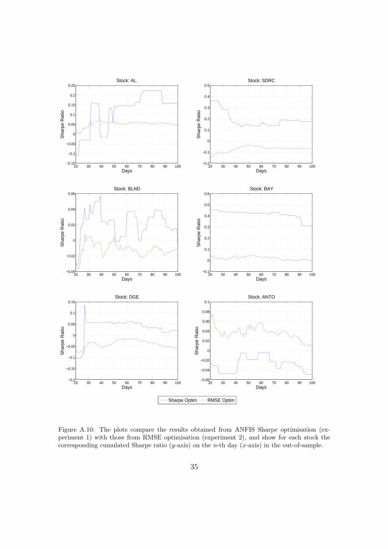
In our final part of this paper we present the results attained from benchmarkmodels that are typically found in literature or used in practice (see overview inTable 4). In the first set of simulations in experiment 2, we applied a RMSEminimisation approach for our model selection process. The results in Table 12show that in the case of ANFIS only two (AL. and ANTO) out of six stocksgenerate positive results; in the case of DENFIS no stock generates a positiveresult; and in the case of FFN only three stocks (AL., BLND and SDRC) generatepositive results. When comparing these results against the results attained by therisk-return based models discussed earlier (in experiment 1), we find that for bothANFIS and DENFIS models the RMSE optimisation provides better results onlyon ANTO. In Figure A.10 we are displaying this for ANFIS over the full out-of-sample period. In the case of FFN, RMSE optimisation clearly outperforms Sharpeoptimisation only in AL. These results are in line with Brabazon and O’Neill (2006)and provide clear indication that trading models based on risk-return selectioncriterion outperform those based on RMSE optimisation.
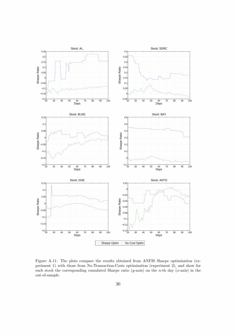
The recent survey by Krollner et al. (2010) identified that most studies do notconsider real world constraints like trading costs (see also Alvarez Dıaz, 2010). Inour second sets of simulations in experiment 2, we base our model selection cri-teria on Sharpe ratio but exclude transaction costs in the training period. In our100 day out-of-sample evaluation, we then apply transaction costs to the selected
25
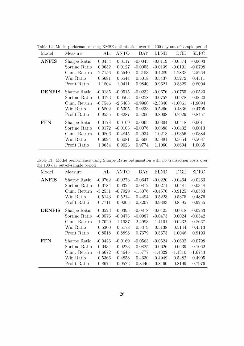
Table 12: Model performance using RMSE optimisation over the 100 day out-of-sample period
Model Measure AL. ANTO BAY BLND DGE SDRC
ANFIS Sharpe Ratio 0.0454 0.0117 -0.0045 -0.0119 -0.0574 -0.0693Sortino Ratio 0.0652 0.0127 -0.0055 -0.0139 -0.0191 -0.0798Cum. Return 2.7156 0.5540 -0.2153 -0.4289 -1.2838 -2.5264Win Ratio 0.5681 0.5544 0.5018 0.5437 0.5272 0.4511Profit Ratio 1.1804 1.0411 0.9840 0.9621 0.8329 0.8004
DENFIS Sharpe Ratio -0.0135 -0.0515 -0.0232 -0.0676 -0.0755 -0.0523Sortino Ratio -0.0123 -0.0503 -0.0258 -0.0752 -0.0978 -0.0620Cum. Return -0.7546 -2.5468 -0.9960 -2.3346 -1.6061 -1.9094Win Ratio 0.5802 0.5305 0.9233 0.5266 0.4836 0.4705Profit Ratio 0.9535 0.8287 0.5206 0.8008 0.7929 0.8457
FFN Sharpe Ratio 0.0178 -0.0109 -0.0065 0.0304 -0.0418 0.0011Sortino Ratio 0.0172 -0.0103 -0.0076 0.0388 -0.0432 0.0013Cum. Return 0.9866 -0.4845 -0.2934 1.0218 -0.9356 0.0384Win Ratio 0.6094 0.6081 0.5606 0.5891 0.5654 0.5087Profit Ratio 1.0654 0.9623 0.9774 1.1060 0.8694 1.0035
Table 13: Model performance using Sharpe Ratio optimisation with no transaction costs overthe 100 day out-of-sample period
Model Measure AL. ANTO BAY BLND DGE SDRC
ANFIS Sharpe Ratio -0.0762 -0.0273 -0.0647 -0.0220 -0.0464 -0.0263Sortino Ratio -0.0784 -0.0325 -0.0872 -0.0271 -0.0481 -0.0348Cum. Return -3.2531 -0.7929 -1.8076 -0.4576 -0.9125 -0.6583Win Ratio 0.5143 0.5214 0.4494 0.5223 0.5375 0.4876Profit Ratio 0.7711 0.9205 0.8207 0.9383 0.8595 0.9255
DENFIS Sharpe Ratio -0.0523 -0.0395 -0.0878 -0.0425 0.0018 -0.0263Sortino Ratio -0.0576 -0.0473 -0.0987 -0.0473 0.0024 -0.0342Cum. Return -1.7020 -1.1937 -2.4993 -1.4101 0.0232 -0.8667Win Ratio 0.5300 0.5178 0.5379 0.5138 0.5144 0.4513Profit Ratio 0.8518 0.8898 0.7679 0.8673 1.0046 0.9193
FFN Sharpe Ratio -0.0426 -0.0169 -0.0563 -0.0524 -0.0602 -0.0798Sortino Ratio -0.0434 -0.0223 -0.0825 -0.0626 -0.0639 -0.1062Cum. Return -1.6672 -0.4645 -1.5777 -1.4322 -1.1810 -1.6743Win Ratio 0.5366 0.4858 0.4630 0.4949 0.5482 0.4905Profit Ratio 0.8674 0.9522 0.8446 0.8460 0.8199 0.7976
26
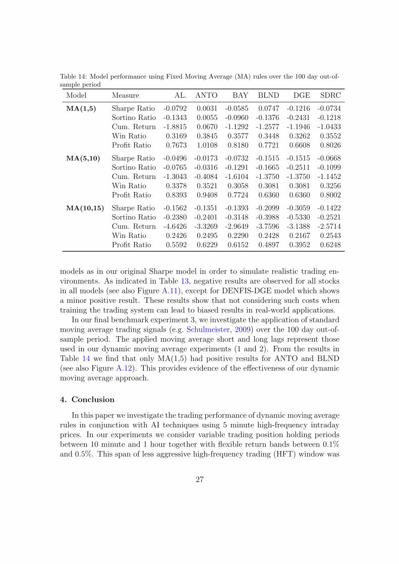
Table 14: Model performance using Fixed Moving Average (MA) rules over the 100 day out-of-sample period
Model Measure AL. ANTO BAY BLND DGE SDRC
MA(1,5) Sharpe Ratio -0.0792 0.0031 -0.0585 0.0747 -0.1216 -0.0734Sortino Ratio -0.1343 0.0055 -0.0960 -0.1376 -0.2431 -0.1218Cum. Return -1.8815 0.0670 -1.1292 -1.2577 -1.1946 -1.0433Win Ratio 0.3169 0.3845 0.3577 0.3448 0.3262 0.3552Profit Ratio 0.7673 1.0108 0.8180 0.7721 0.6608 0.8026
MA(5,10) Sharpe Ratio -0.0496 -0.0173 -0.0732 -0.1515 -0.1515 -0.0668Sortino Ratio -0.0765 -0.0316 -0.1291 -0.1665 -0.2511 -0.1099Cum. Return -1.3043 -0.4084 -1.6104 -1.3750 -1.3750 -1.1452Win Ratio 0.3378 0.3521 0.3058 0.3081 0.3081 0.3256Profit Ratio 0.8393 0.9408 0.7724 0.6360 0.6360 0.8002
MA(10,15) Sharpe Ratio -0.1562 -0.1351 -0.1393 -0.2099 -0.3059 -0.1422Sortino Ratio -0.2380 -0.2401 -0.3148 -0.3988 -0.5330 -0.2521Cum. Return -4.6426 -3.3269 -2.9649 -3.7596 -3.1388 -2.5714Win Ratio 0.2426 0.2495 0.2290 0.2428 0.2167 0.2543Profit Ratio 0.5592 0.6229 0.6152 0.4897 0.3952 0.6248
models as in our original Sharpe model in order to simulate realistic trading en-vironments. As indicated in Table 13, negative results are observed for all stocksin all models (see also Figure A.11), except for DENFIS-DGE model which showsa minor positive result. These results show that not considering such costs whentraining the trading system can lead to biased results in real-world applications.
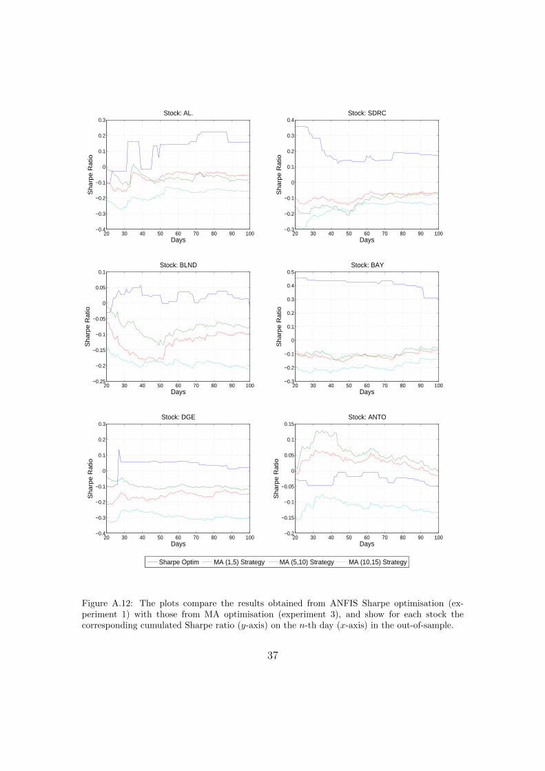
In our final benchmark experiment 3, we investigate the application of standardmoving average trading signals (e.g. Schulmeister, 2009) over the 100 day out-of-sample period. The applied moving average short and long lags represent thoseused in our dynamic moving average experiments (1 and 2). From the results inTable 14 we find that only MA(1,5) had positive results for ANTO and BLND(see also Figure A.12). This provides evidence of the effectiveness of our dynamicmoving average approach.
4. Conclusion
In this paper we investigate the trading performance of dynamic moving averagerules in conjunction with AI techniques using 5 minute high-frequency intradayprices. In our experiments we consider variable trading position holding periodsbetween 10 minute and 1 hour together with flexible return bands between 0.1%and 0.5%. This span of less aggressive high-frequency trading (HFT) window was
27
chosen to gain more insight on the profitability of intraday trading with respect tothe tension created between two literature findings: (i) the view that profitabilityof trading rules has possibly moved to higher frequency prices (Schulmeister, 2009),and on the other hand, (ii) the view that aggressive HFT with position holdingperiods between 10 milliseconds and 10 seconds does not reap the expected excessreturns (Kearns et al., 2010).
We consider the traditional ANN as well as the more recent ANFIS and DEN-FIS models. Our results, based on applying a trading algorithm to a set of stockslisted on the London Stock Exchange, show that the application of these modelscan be used to support profitable trading strategies. The sensitivity analysis of ourmodels with respect to holding position time and return band provide clear indi-cation that financial markets are not fully efficient at less aggressive HFT windowsand there exist temporary “pockets of predictability” which could be exploited forrealising excess returns.
In our out-of-sample evaluation, we show that overall FFN models performwell when compared with the more recent Neuro Fuzzy techniques. However, FFNmodels also show higher sensitivity to the underlying data features. Looking at the100 day aggregated trading performance, we find that ANFIS provides the mostrobust performance measure exhibiting least variance, both in the case of Sharpeand Sortino ratios optimisation. In our experiments, DENFIS did not outperformFFN and ANFIS (see also Tan et al., 2011). Results also show that ANNs stillprovide a valid benchmark when applying more recent Neuro-Fuzzy models onhigh frequency price series.
Our results indicate that the selection of specific risk-return measures does nothave the same effect on the behaviour of the underlying AI technique and doesnot guarantee the same time varying performance across all models. Hence theselection of the risk-return optimisation measure has to be based on the investorrisk profile, the underlying technique being applied and the dynamic nature of theunderlying price distribution.
This validates the importance of investigating the time varying daily time-series profile of the cumulative risk-return measures attained when evaluating theunderlying models for investment decisions rather than just looking at performancemeasures following an arbitrary out of sample period. Simple risk-free metrics usedfrequently in literature such as percentage of successful trades only convey littleinformation on the actual profitability of the algorithm.
We also compare our models with a set of benchmark models commonly foundin literature or used in practice (Krollner et al., 2010). Our results show thattrading models based on risk-return selection criterion outperform those based onRMSE optimisation. In the second comparison we base our model selection criteriaon Sharpe ratio but exclude transaction costs, a feature that most studies do not
28
consider, possibly reporting overestimated profitability. In our final comparison,we investigate the application of fixed moving average trading signals. Again theresults here did not outperform our dynamic moving average approach.
Another area of interesting research is the application of heat maps to identifyregions of profitable areas and how these regions change with time. These findingsalso encourage further research into stacked models which involve the combinationof different AI models in an investment decision portfolio with varying risk-returnfeatures.
Acknowledgement
The authors would like to thank Hani Hagras and Edward Tsang for theirvaluable feedback and helpful discussions.
References
Alvarez Dıaz, M. (2010). Speculative strategies in the foreign exchange mar-ket based on genetic programming predictions. Applied Financial Economics,20(6):465–476.
Alves Portela Santos, A., Carneiro Affonso da Costa, N., and dos Santos Coelho, L.(2007). Computational intelligence approaches and linear models in case studiesof forecasting exchange rates. Expert Systems with Applications, 33(4):816–823.
Brabazon, A. and O’Neill, M. (2006). Biologically inspired algorithms for financialmodelling, volume 20. Springer Berlin.
Choey, M. and Weigend, A. S. (1997). Nonlinear trading models through sharperatio maximization. International Journal of Neural Systems, 8(04):417–431.
de Faria, E., Albuquerque, M. P., Gonzalez, J., Cavalcante, J., and Albuquerque,M. P. (2009). Predicting the Brazilian stock market through neural networksand adaptive exponential smoothing methods. Expert Systems with Applications,36(10):12506–12509.
Enke, D. and Thawornwong, S. (2005). The use of data mining and neural net-works for forecasting stock market returns. Expert Systems with Applications,29(4):927–940.
Fernandez-Rodrıguez, F., Gonzalez-Martel, C., and Sosvilla-Rivero, S. (2000). Onthe profitability of technical trading rules based on artificial neural networks:Evidence from the Madrid stock market. Economics Letters, 69(1):89–94.
29
Gencay, R. (1996). Non-linear prediction of security returns with moving averagerules. Journal of Forecasting, 15(3):165–174.
Gradojevic, N. (2007). Non-linear, hybrid exchange rate modeling and tradingprofitability in the foreign exchange market. Journal of Economic Dynamicsand Control, 31(2):557–574.
Hudson, R., Dempsey, M., and Keasey, K. (1996). A note on the weak formefficiency of capital markets: The application of simple technical trading rulesto UK stock prices-1935 to 1994. Journal of Banking & Finance, 20(6):1121–1132.
Jang, J. (1993). ANFIS: Adaptive-network-based fuzzy inference system. IEEETransactions on Systems, Man and Cybernetics, 23(3):665–685.
Kablan, A. and Ng, W. (2011). Intraday high-frequency FX trading with adaptiveneuro-fuzzy inference systems. International Journal of Financial Markets andDerivatives, 2(1):68–87.
Kasabov, N. and Filev, D. (2006). Evolving intelligent systems: methods, learning,& applications. In 2006 International Symposium on Evolving Fuzzy Systems,pages 8–18. IEEE.
Kasabov, N. and Song, Q. (2002). DENFIS: dynamic evolving neural-fuzzy infer-ence system and its application for time-series prediction. IEEE Transactionson Fuzzy Systems, 10(2):144–154.
Kearns, M., Kulesza, A., and Nevmyvaka, Y. (2010). Empirical limitations onHigh-Frequency Trading Profitability. The Journal of Trading, 5(4):50–62.
Krollner, B., Vanstone, B., and Finnie, G. (2010). Financial time series forecastingwith machine learning techniques: A survey. In 2011 proceedings, Europeansymposium on artificial neural networks: Computational and machine learning,Bruges (Belgium), pages 28–30.
Lin, C., Khan, H., and Huang, C. (2002). Can the neuro fuzzy model predict stockindexes better than its rivals? CIRJE F-Series.
Marsland, S. (2009). Machine Learning: an Algorithmic Perspective. Chapman &Hall/CRC.
Medeiros, M. C., Terasvirta, T., and Rech, G. (2006). Building neural networkmodels for time series: a statistical approach. Journal of Forecasting, 25(1):49–75.
30
Resta, M. (2009). Seize the (intra)day: Features selection and rules extraction fortradings on high-frequency data. Neurocomputing, 72(16-18):3413–3427.
Schulmeister, S. (2009). Profitability of technical stock trading: Has it moved fromdaily to intraday data? Review of Financial Economics, 18(4):190–201.
Son, Y., Noh, D.-j., and Lee, J. (2012). Forecasting trends of high-frequencyKOSPI200 index data using learning classifiers. Expert Systems with Applica-tions, 39(14):11607–11615.
Takagi, T. and Sugeno, M. (1985). Fuzzy identification of systems and its appli-cations to modeling and control. Systems, Man and Cybernetics, IEEE Trans-actions on, (1):116–132.
Tan, Z., Quek, C., and Cheng, P. Y. (2011). Stock trading with cycles: A fi-nancial application of ANFIS and reinforcement learning. Expert Systems withApplications, 38(5):4741–4755.
Tsai, C. and Wang, S. (2009). Stock price forecasting by hybrid machine learningtechniques. In Proceedings of the International MultiConference of Engineersand Computer Scientists, volume 1, pages 755–760.
Tsang, E. (2009). Forecasting where computational intelligence meets the stockmarket. Frontiers of Computer Science in China, 1(3):53–63.
Vanstone, B. and Finnie, G. (2009). An empirical methodology for developingstockmarket trading systems using artificial neural networks. Expert Systemswith Applications, 36(3):6668–6680.
Vanstone, B. and Finnie, G. (2010). Enhancing stockmarket trading performancewith ANNs. Expert Systems with Applications, 37(9):6602–6610.
Xufre Casqueiro, P. and Rodrigues, A. J. (2006). Neuro-dynamic trading methods.European journal of operational research, 175(3):1400–1412.
Zadeh, L. (1975). The concept of a linguistic variable and its application to ap-proximate reasoning – Part I. Information Sciences, 8(3):199–249.
Appendix A. Appendix
31
20 30 40 50 60 70 80 90 1000
0.5
1
1.5
2Stock: AL.
Days
Pro
fit R
atio
20 30 40 50 60 70 80 90 1000.5
1
1.5
2
2.5
3Stock: SDRC
Days
Pro
fit R
atio
20 30 40 50 60 70 80 90 1000
0.5
1
1.5
2
2.5
3
3.5
4Stock: BLND
Days
Pro
fit R
atio
20 30 40 50 60 70 80 90 1001.5
2
2.5
3
3.5
4
4.5
5
5.5
6Stock: BAY
Days
Pro
fit R
atio
20 30 40 50 60 70 80 90 1000
0.5
1
1.5
2
2.5Stock: DGE
Days
Pro
fit R
atio
20 30 40 50 60 70 80 90 100
0.8
1
1.2
1.4
1.6
1.8
2Stock: ANTO
Days
Pro
fit R
atio
ANFIS−So ANFIS−Sh DENFIS−So DENFIS−Sh FFN−So FFN−Sh
Figure A.7: Profit ratio performance of ANFIS-Sharpe (ANF-Sh), ANFIS-Sortino (ANF-So),DENFIS-Sharpe (DEN-Sh), DENFIS-Sortino (DEN-So), FFN-Sharpe (FFN-Sh) and FFN-Sortino (FFN-So) models. The plots show for each stock the cumulated profit ratio (y-axis)on the n-th day (x-axis) in the out-of-sample.
32
20 30 40 50 60 70 80 90 100−0.2
−0.1
0
0.1
0.2
0.3
0.4
0.5Stock: AL.
Days
Cum
ulat
ive
Ret
urn
20 30 40 50 60 70 80 90 100−0.4
−0.3
−0.2
−0.1
0
0.1
0.2
0.3
0.4
0.5Stock: SDRC
Days
Cum
ulat
ive
Ret
urn
20 30 40 50 60 70 80 90 100−0.15
−0.1
−0.05
0
0.05
0.1
0.15
0.2Stock: BLND
Days
Cum
ulat
ive
Ret
urn
20 30 40 50 60 70 80 90 100
0.2
0.25
0.3
0.35
0.4
0.45
0.5Stock: BAY
Days
Cum
ulat
ive
Ret
urn
20 30 40 50 60 70 80 90 100−0.05
0
0.05
0.1
0.15
0.2
0.25
0.3
0.35
0.4Stock: DGE
Days
Cum
ulat
ive
Ret
urn
20 30 40 50 60 70 80 90 100−0.25
−0.2
−0.15
−0.1
−0.05
0
0.05
0.1
0.15
0.2Stock: ANTO
Days
Cum
ulat
ive
Ret
urn
ANFIS−So ANFIS−Sh DENFIS−So DENFIS−Sh FFN−So FFN−Sh
Figure A.8: Cumulative Return performance of ANFIS-Sharpe (ANF-Sh), ANFIS-Sortino (ANF-So), DENFIS-Sharpe (DEN-Sh), DENFIS-Sortino (DEN-So), FFN-Sharpe (FFN-Sh) and FFN-Sortino (FFN-So) models. The plots show for each stock the cumulated return (y-axis) on then-th day (x-axis) in the out-of-sample.
33
20 30 40 50 60 70 80 90 1000.1
0.2
0.3
0.4
0.5
0.6
0.7
0.8Stock: AL.
Days
Win
Rat
io
20 30 40 50 60 70 80 90 1000.35
0.4
0.45
0.5
0.55
0.6
0.65
0.7
0.75Stock: SDRC
Days
Win
Rat
io
20 30 40 50 60 70 80 90 1000.2
0.3
0.4
0.5
0.6
0.7
0.8
0.9Stock: BLND
Days
Win
Rat
io
20 30 40 50 60 70 80 90 1000.5
0.55
0.6
0.65
0.7Stock: BAY
Days
Win
Rat
io
20 30 40 50 60 70 80 90 1000.35
0.4
0.45
0.5
0.55
0.6
0.65
0.7Stock: DGE
Days
Win
Rat
io
20 30 40 50 60 70 80 90 1000.46
0.48
0.5
0.52
0.54
0.56
0.58
0.6
0.62Stock: ANTO
Days
Win
Rat
io
ANFIS−So ANFIS−Sh DENFIS−So DENFIS−Sh FFN−So FFN−Sh
Figure A.9: Win ratio performance of ANFIS-Sharpe (ANF-Sh), ANFIS-Sortino (ANF-So),DENFIS-Sharpe (DEN-Sh), DENFIS-Sortino (DEN-So), FFN-Sharpe (FFN-Sh) and FFN-Sortino (FFN-So) models (out-of-sample). The plots show for each stock the cumulated winratio (y-axis) on the n-th day (x-axis) in the out-of-sample.
34
20 30 40 50 60 70 80 90 100−0.15
−0.1
−0.05
0
0.05
0.1
0.15
0.2
0.25Stock: AL.
Days
Sh
arp
e R
atio
20 30 40 50 60 70 80 90 100−0.2
−0.1
0
0.1
0.2
0.3
0.4
0.5Stock: SDRC
Days
Sh
arp
e R
atio
20 30 40 50 60 70 80 90 100−0.04
−0.02
0
0.02
0.04
0.06Stock: BLND
Days
Sh
arp
e R
atio
20 30 40 50 60 70 80 90 100−0.1
0
0.1
0.2
0.3
0.4
0.5
0.6Stock: BAY
Days
Sh
arp
e R
atio
20 30 40 50 60 70 80 90 100−0.2
−0.15
−0.1
−0.05
0
0.05
0.1
0.15Stock: DGE
Days
Sh
arp
e R
atio
20 30 40 50 60 70 80 90 100−0.06
−0.04
−0.02
0
0.02
0.04
0.06
0.08
0.1Stock: ANTO
Days
Sh
arp
e R
atio
Sharpe Optim RMSE Optim
Figure A.10: The plots compare the results obtained from ANFIS Sharpe optimisation (ex-periment 1) with those from RMSE optimisation (experiment 2), and show for each stock thecorresponding cumulated Sharpe ratio (y-axis) on the n-th day (x-axis) in the out-of-sample.
35
20 30 40 50 60 70 80 90 100−0.2
−0.15
−0.1
−0.05
0
0.05
0.1
0.15
0.2
0.25Stock: AL.
Days
Sh
arp
e R
atio
20 30 40 50 60 70 80 90 100−0.05
0
0.05
0.1
0.15
0.2
0.25
0.3
0.35
0.4Stock: SDRC
Days
Sh
arp
e R
atio
20 30 40 50 60 70 80 90 100−0.2
−0.15
−0.1
−0.05
0
0.05
0.1
0.15Stock: BLND
Days
Sh
arp
e R
atio
20 30 40 50 60 70 80 90 100−0.1
0
0.1
0.2
0.3
0.4
0.5
0.6Stock: BAY
Days
Sh
arp
e R
atio
20 30 40 50 60 70 80 90 100−0.2
−0.15
−0.1
−0.05
0
0.05
0.1
0.15Stock: DGE
Days
Sh
arp
e R
atio
20 30 40 50 60 70 80 90 100−0.14
−0.12
−0.1
−0.08
−0.06
−0.04
−0.02
0
0.02Stock: ANTO
Days
Sh
arp
e R
atio
Sharpe Optim No Cost Optim
Figure A.11: The plots compare the results obtained from ANFIS Sharpe optimisation (ex-periment 1) with those from No-Transaction-Costs optimisation (experiment 2), and show foreach stock the corresponding cumulated Sharpe ratio (y-axis) on the n-th day (x-axis) in theout-of-sample.
36
20 30 40 50 60 70 80 90 100−0.4
−0.3
−0.2
−0.1
0
0.1
0.2
0.3Stock: AL.
Days
Sh
arp
e R
atio
20 30 40 50 60 70 80 90 100−0.3
−0.2
−0.1
0
0.1
0.2
0.3
0.4Stock: SDRC
Days
Sh
arp
e R
atio
20 30 40 50 60 70 80 90 100−0.25
−0.2
−0.15
−0.1
−0.05
0
0.05
0.1Stock: BLND
Days
Sh
arp
e R
atio
20 30 40 50 60 70 80 90 100−0.3
−0.2
−0.1
0
0.1
0.2
0.3
0.4
0.5Stock: BAY
Days
Sh
arp
e R
atio
20 30 40 50 60 70 80 90 100−0.4
−0.3
−0.2
−0.1
0
0.1
0.2
0.3Stock: DGE
Days
Sh
arp
e R
atio
20 30 40 50 60 70 80 90 100−0.2
−0.15
−0.1
−0.05
0
0.05
0.1
0.15Stock: ANTO
Days
Sh
arp
e R
atio
Sharpe Optim MA (1,5) Strategy MA (5,10) Strategy MA (10,15) Strategy
Figure A.12: The plots compare the results obtained from ANFIS Sharpe optimisation (ex-periment 1) with those from MA optimisation (experiment 3), and show for each stock thecorresponding cumulated Sharpe ratio (y-axis) on the n-th day (x-axis) in the out-of-sample.
37