Embed Size (px)
DESCRIPTION
Bank of Portigal: “Unpleasant debt dynamics: Can fiscal consolidations raise debt ratios?”
Citation preview

UNPLEASANT DEBT DYNAMICS: CAN FISCAL CONSOLIDATIONS RAISE DEBT RATIOS?
Working Papers 2015Gabriela Castro | Ricardo M. Félix | Paulo Júlio | José R. Maria
1


UNPLEASANT DEBT DYNAMICS: CAN FISCAL CONSOLIDATIONS RAISE DEBT RATIOS?
Working Papers 2015
Gabriela Castro | Ricardo M. Félix | Paulo Júlio | José R. Maria
Lisbon, 2015 • www.bportugal.pt
1
February 2015The analyses, opinions and findings of these papers represent the views of the authors, they are not necessarily those of the Banco de Portugal or the Eurosystem
Please address correspondence toBanco de Portugal, Economics and Research Department Av. Almirante Reis 71, 1150-012 Lisboa, PortugalT +351 213 130 000 | [email protected]

WORKING PAPERS | Lisbon 2015 • Banco de Portugal Av. Almirante Reis, 71 | 1150-012 Lisboa • www.bportugal.pt •
Edition Economics and Research Department • ISBN 978-989-678-329-7 (online) • ISSN 2182-0422 (online)
Unpleasant debt dynamics:
Can fiscal consolidations raise debt ratios?∗
Gabriela Castro† Ricardo M. Felix† Paulo Julio‡ Jose R. Maria†
February 20, 2015
Abstract
Using PESSOA, a medium-scale DSGE model for a small euro-area economy, we
evaluate how fiscal adjustments impact short- and medium-term debt dynamics and
output for alternative policy options, and budgetary and economic conditions. Fiscal
adjustments may increase the public debt-to-GDP ratio in the short run, even for
consolidations carried out in normal times in economies characterized by moderate
indebtedness levels. Financial turmoils and hikes in the nationwide risk premia, cou-
pled with high indebtedness levels and stiff fiscal measures, boost the output costs of
fiscal consolidations and severely affect their effectiveness in bringing the public debt-
to-GDP ratio down in the short term. In the medium run credible fiscal adjustments
entail a decline in the public debt ratio, though at potentially very large output losses
when carried out under unfavorable budgetary and economic conditions.
JEL Classification: E12, E30, E62, H60
Keywords: Fiscal policy, Fiscal consolidation, Debt ratio, crisis, DSGE model, Euro
Area, Small open economy
1 Introduction
The short-run impact of fiscal policies on the public debt-to-GDP ratio (hereinafter termed
debt ratio) was not considered a key issue in developed countries until the inception of
the Great Recession. Though fiscal consolidation has long been in the political agenda of
European fiscal authorities, the existence of an apparently mechanical negative relationship
between the consolidation effort and the debt ratio dictated the mild relevance of the
topic. The change in the economic environment brought about by the Great Recession
∗We thank the comments of Pietro Cova, Lara Wemans, Hugo Vilares, Luıs Fonseca, and of all par-ticipants in the 2014 Central Bank Macroeconomic Modeling Workshop (Rome, October 2014). PauloJulio is pleased to acknowledge financial support from Fundacao para a Ciencia e a Tecnologia andFEDER/COMPETE (grant PEst-C/EGE/UI4007/2013). The views expressed in this article are thoseof the authors and do not necessarily reflect the views of Banco de Portugal or the Eurosystem. Any errorsand mistakes are ours.†Economics and Research Department, Banco de Portugal.‡Economics and Research Department, Banco de Portugal; and Center for Advanced Studies in Man-
agement and Economics, Portugal. Corresponding author. Address: Rua Francisco Ribeiro, 2, 1150–165Lisboa. E-mail: [email protected]
1

changed the panorama. In an attempt to offset the adverse effects of the 2008 Financial
Crisis on aggregate demand and thus on output, fiscal stimulus programmes were adopted
worldwide. The debt ratio in the European Union increased from 59 percent in 2007
to 80 percent in 2010, and a similar development was experienced in the Euro Area as
a whole, though some peripheral countries presented larger increments. By that time
it was already clear that public debt was approaching an unsustainable level in some
economies according to market participants, as suggested by the hike in sovereign debt
spreads and credit default swaps. Expansionary fiscal policies therefore gave way to harsh
consolidation strategies, aimed at restoring sovereign credibility and bringing down public
debt. The effectiveness of such policies was limited at best, with debt ratios maintaining
an upward trend, particularly in countries characterized by high indebtedness levels and
engaging in harsh and front-loaded consolidation strategies. The prime examples are
Ireland, Greece, and Portugal—countries which registered sharp increases in the debt ratio
between 2010 and 2012, despite the implementation of financial assistance programmes
implying stiff consolidation measures. Such outcome triggered the debate, both in the
economics profession and in the media, about the effectiveness of fiscal adjustments in
turbulent periods.1
Whether fiscal adjustments are able to put an halt to an upward trend in the debt
ratio or even to revert it depends solely on the interaction between the consolidation
effort—specifically the decline in the primary deficit ratio—and the strength of the so-
called snowball effect—the increase in the value of the outstanding debt ratio induced by
the wedge between the nationwide real interest rate and real GDP growth.2 A higher
nominal interest rate raises interest outlays; a decline in GDP inflation boosts the real
value of outstanding debt; and lower real GDP growth brings up the value of outstanding
debt vis-a-vis the economy’s real income.3
Using PESSOA, a medium-scale Dynamic Stochastic General Equilibrium (DSGE)
model for a small euro-area economy encompassing non-Ricardian agents, nominal and
real rigidities, and financial frictions, we study the dynamics of debt and output that follow
credible fiscal consolidations for alternative policy options—namely different instrument
mixes and consolidation paces—and budgetary conditions—viz initial indebtedness and
fiscal effort levels. We address also the role played by changes in the economic environment,
specifically temporary increases in the nationwide risk premia and financially induced
crisis. It is worth emphasizing that our exercise does not aim at discussing whether fiscal
adjustments should be pursued nor addresses the optimal debt target; we assume from
1See, for instance, the debate taking place at the Vox (http://www.voxeu.org).2The long-run effects of fiscal consolidation is a topic with completely different implications, which we
do not discuss here. For the long-run benefits of fiscal consolidation see Rother, Schuknecht, and Stark(2010), Mulas-Granados, Baldacci, and Gupta (2010), Barrios, Langedijk, and Pench (2010) and Almeidaet al. (2013b).
3Fiscal consolidations leading to temporary increases in the debt ratio are often labeled in the literatureas “self-defeating” fiscal consolidations (e.g. Boussard, Castro, and Salto 2013, Berti, De Castro, andSalto 2013, Eyraud and Weber 2013), though we avoid this wording throughout the article. It is ourunderstanding that this expression appeals to the impossibility of bringing the debt ratio down at all, i.e.a defeat of consolidation measures due to unsustainable debt dynamics.
2

the outset that fiscal authorities are forced to carry out a given fiscal consolidation plan.4
Moreover, we address only the case wherein fiscal adjustments are fully credible, i.e. fiscal
authorities commit to lower the debt ratio to a new target level, and this is immediately
taken into account by all economic agents.
We show that the snowball effect—triggered by the decline in real GDP growth and
inflation—can outweigh the consolidation effort and bring about an increase in the debt ra-
tio in the short term. This outcome may hold under regular conditions—for consolidations
carried out in normal times in economies characterized by moderate indebtedness levels—
but it is substantially amplified by the initial outstanding debt ratio and the fiscal effort
level. A higher initial outstanding debt ratio boosts the snowball effect. A larger effort
level triggers a steeper decline in nominal GDP and thus a stronger snowball effect, whose
short-run impact on the debt ratio may outweigh that of the stiffer adjustment. Fiscal
consolidations performed in periods of crisis and preceded by hikes in the nationwide risk
premia place a natural upward pressure in the snowball effect and thus in the debt ratio,
forcing fiscal authorities to enlarge the fiscal package to comply with the new fiscal target.
Stiffer consolidation measures, jointly with the unfavorable economic environment, entail
larger output losses and pressure the debt ratio further upwards. In the medium run,
credible fiscal adjustments successfully lower the debt ratio, though at potentially large
output losses when carried out under unfavorable budgetary and economic conditions.
Output losses can be mitigated if expenditure-side measures and back-loaded adjustments
are used instead of revenue-side measures—which depress output for a protracted time pe-
riod due to important distortionary effects—and front-loaded adjustments—which trigger
more severe slumps. Expenditure-side measures and back-loaded adjustments generally
entail, however, a larger short-run increase in the debt ratio.5
Our conclusions therefore hint that the hike in the nationwide risk premia and the
decline in real GDP growth brought about by the Great Recession, coupled with high
indebtedness levels registered throughout the turmoil and the stiff fiscal retrenchment that
was carried out meanwhile, may have boosted the output losses of fiscal consolidations and
severely affected their effectiveness in bringing the public debt ratio down vis-a-vis the
pre-crisis period.
The article contributes towards the literature in at least two key dimensions. First,
to our best knowledge, no other study explicitly addresses short-run debt dynamics in a
medium-scale DSGE model. There are a few studies on the subject, but they rely solely
on the equation for the law of motion of the debt ratio, an approach often requiring some
assumptions as regards to the output effects of fiscal consolidations (e.g. Boussard, Castro,
and Salto 2013, Eyraud and Weber 2013). Moreover, the role of inflation is often ignored
in these studies, though it affects the real value of (non-contingent) debt and thus the
4The consequences of avoiding or postponing a pressing fiscal adjustment is a completely different topicwhich lies outside the scope of this article.
5Back-loaded fiscal adjustments may entail credibility issues, triggering hikes in the nationwide riskpremia that adversely affect both the debt ratio and output. Under such environment, front-loaded con-solidations may be preferred to back-loaded ones if credibility is at stake. Back-loaded adjustments couldbe made credible through the adoption of multiannual budget plans that enjoy a broad political support.
3

debt ratio. Second, the spectrum of our analysis—encompassing the main drivers of the
law of motion of debt as well as their interactions—captures key changes in economic and
budgetary features brought about by the Great Recession, which, to our best knowledge,
have not yet been jointly addressed elsewhere. The literature focuses mostly on the role
played by the size of fiscal multipliers on debt dynamics, leaving aside other relevant
factors and their interactions.
This article is organized as follows. Section 2 briefly reviews selected literature. Section
3 shortly describes the model. Section 4 presents the law of motion of the debt ratio
within the context of PESSOA, and describes the fiscal consolidation exercise. Section 5
and Section 6 present and discuss the results. Section 7 concludes.
2 Literature overview
The bottom line amongst the articles that address short-run debt dynamics lies on the
size of fiscal multipliers, which are likely to be larger in periods of crisis. Fiscal gains in
crisis times may be wiped out by the decline in output, leading to short-run increases in
the debt ratio that can last for several years, as argued by Boussard, Castro, and Salto
(2013) and Eyraud and Weber (2013). The former study simulates debt paths under
different economic characterizations after pinning down the equations characterizing debt
dynamics. The latter performs a similar exercise, but complements the analysis with an
empirical approach. The impact on the debt ratio is exacerbated if financial markets
focus on short-term performance or are characterized by a substantial degree of myopia.
Berti, De Castro, and Salto (2013) analyze the effects of fiscal consolidation envisaged in
the 2013 Stability and Convergence Programmes presented by European Union Member
States, under different assumptions on the underlying fiscal multipliers. The authors
conclude that large fiscal multipliers entail temporary increases in the debt ratio following
fiscal consolidation measures.
Along similar lines, Padoan, Sila, and van den Noord (2012) argue that some economies
may be trapped in a bad equilibria, characterized by the simultaneous occurrence of high
growing fiscal deficits and debt, high risk premia on sovereign debt, slumping economic
activity, and plummeting confidence, all of which endowed with adverse feedback effects.
In the short run the negative impact on demand may adversely affect market confidence
to the extent that it depresses growth, hence affecting debt sustainability.
The effects on output can be minimized if smooth and gradual consolidations are pre-
ferred to front-loaded or aggressive ones, because sheltering economic activity is key to
success. As a result, implementing fiscal consolidations in more favorable times, during
periods of positive GDP growth, significantly reduces the impact of fiscal tightening mea-
sures on output. This argument is illustrated by Batini, Callegari, and Melina (2012)
and Cherif and Hasanov (2012), the former using a threshold VAR structure to capture
asymmetric macroeconomic developments during expansions and downturns, and the lat-
ter using a modified VAR framework with debt feedback effects, which suggests that the
4

likelihood of a short-run increase in the debt-to-GDP ratio is much higher under weak
economic conditions.
On the theoretical front, the few articles that focus on short-run debt dynamics simply
pin down the equation for the law of motion of the debt ratio, given exogenous param-
eterizations for fiscal multipliers, initial debt, and interest rate developments (Boussard,
Castro, and Salto 2013, Berti, De Castro, and Salto 2013, Eyraud and Weber 2013). This
approach poses an important limitation, since one cannot properly take into account the
feedback effects from the economic environment to the debt ratio, nor the specific design
of fiscal policy measures. In addition, the understanding of the effects at work is rather
limited. Forni, Monteforte, and Sessa (2009) develop and estimate a medium-scale DSGE
model for the Euro Area to analyze the response of macro variables to a wide range of
fiscal shocks. However, they do not focus on the debt dynamics of fiscal consolidations.
To our best knowledge, the effects of fiscal adjustments on short- and medium-term
debt dynamics and output for alternative policy options, and budgetary and economic
conditions, have not yet been addressed in a medium-scale DSGE model, wherein all
effects of fiscal shocks are endogenously determined.
3 A model for a small euro-area economy
PESSOA is a New-Keynesian DSGE model for a monetarily-integrated small open econ-
omy. It features a multi-sectoral production structure, non-Ricardian characteristics, im-
perfect market competition, and a number of nominal and real rigidities that allow for re-
alistic short-run dynamics and create room for welfare improving stabilization policies. In
addition, the model contemplates financial frictions a la Bernanke, Gertler, and Gilchrist
(1999), whereby financial shocks are transmitted and propagated to the real economy.
The economy is composed of nine types of agents: households, labor unions, capital
goods producers, entrepreneurs, banks, intermediate goods producers (manufacturers),
final goods producers (distributors), the government, and foreign agents (the rest of the
monetary union). Figure 1 depicts the interactions between agents in PESSOA. The rest
of the section briefly reviews the main features of the model. Additional details can be
found in Almeida, Castro, and Felix (2010), Almeida et al. (2013b). The model’s complete
analytical solution is presented in Almeida et al. (2013a).
A constant number of households evolves according to the overlapping generations
scheme first proposed in Blanchard (1985). They are subject to stochastic finite lifetimes
and face an identical and constant probability of death, independent of age.6 Households
rent labor services to labor unions, receiving in return a productivity adjusted wage rate,
over which they pay a labor income tax. Labor productivity is assumed to decay over
lifetime at a constant rate. Two types of households coexist in the model: asset holders,
who are able to smooth consumption over lifetime by trading assets; and hand-to-mouth
6The probability of death can be also interpreted as the degree of “myopia” (Blanchard 1985, Frenkeland Razin 1996, Harrison et al. 2005, Bayoumi and Sgherri 2006). In other words, the future is seen as aperiod of lesser economic relevance.
5
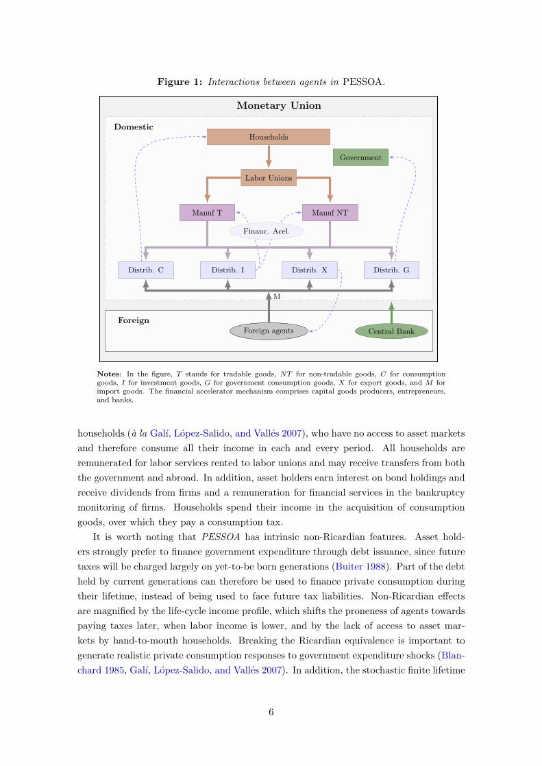
Figure 1: Interactions between agents in PESSOA.
Monetary Union
Domestic
Foreign
Distrib. C Distrib. I Distrib. X Distrib. G
Foreign agents
Manuf T Manuf NT
Labor Unions
Households
Government
Central Bank
M
Financ. Acel.
Notes: In the figure, T stands for tradable goods, NT for non-tradable goods, C for consumptiongoods, I for investment goods, G for government consumption goods, X for export goods, and M forimport goods. The financial accelerator mechanism comprises capital goods producers, entrepreneurs,and banks.
households (a la Galı, Lopez-Salido, and Valles 2007), who have no access to asset markets
and therefore consume all their income in each and every period. All households are
remunerated for labor services rented to labor unions and may receive transfers from both
the government and abroad. In addition, asset holders earn interest on bond holdings and
receive dividends from firms and a remuneration for financial services in the bankruptcy
monitoring of firms. Households spend their income in the acquisition of consumption
goods, over which they pay a consumption tax.
It is worth noting that PESSOA has intrinsic non-Ricardian features. Asset hold-
ers strongly prefer to finance government expenditure through debt issuance, since future
taxes will be charged largely on yet-to-be born generations (Buiter 1988). Part of the debt
held by current generations can therefore be used to finance private consumption during
their lifetime, instead of being used to face future tax liabilities. Non-Ricardian effects
are magnified by the life-cycle income profile, which shifts the proneness of agents towards
paying taxes later, when labor income is lower, and by the lack of access to asset mar-
kets by hand-to-mouth households. Breaking the Ricardian equivalence is important to
generate realistic private consumption responses to government expenditure shocks (Blan-
chard 1985, Galı, Lopez-Salido, and Valles 2007). In addition, the stochastic finite lifetime
6

framework allows for the endogenous determination of the net foreign asset position of the
economy in the steady state, by limiting the amount of assets/debt that households can
accumulate (Harrison et al. 2005). This generates a positive correlation between public
debt and the net foreign debt position, representing thus an appealing feature for the
simulation of permanent fiscal shocks, as is the case of this article.
Labor unions hire labor services from households and sell them to manufacturers op-
erating in the intermediate goods market. They are perfectly competitive in the input
market and monopolistically competitive in the output market, and face adjustment costs
on wage changes. Market power arises from the fact that labor unions supply differenti-
ated, imperfectly substitutable labor services.
Manufacturers combine capital, rented from entrepreneurs, with labor services, hired
from labor unions, to produce an intermediate good, which is thereafter sold to distribu-
tors. There are two types of manufacturers: those producing tradable goods, and those
producing nontradable goods. Manufacturers are perfectly competitive in the input mar-
ket and monopolistically competitive in the output market, and face quadratic adjustment
costs on price changes. They pay social security taxes on their payroll and capital income
taxes on profits.
Distributors combine domestic intermediate goods (both tradable and non-tradable)
with imported goods to produce four types of differentiated final goods. Each type of
final good is acquired by a unique type of costumer: consumption goods are acquired by
households, investment goods by capital goods producers, government consumption goods
by the government, and export goods by foreign distributors. Analogously to manufac-
turers, distributors are perfectly competitive in the input market and monopolistically
competitive in the output market and face quadratic adjustment costs on price changes.
They pay capital income taxes on profits.
Capital goods producers are the exclusive producers of capital. Before each produc-
tion cycle, they buy the undepreciated capital from entrepreneurs and combine it with
investment goods bought from distributors to produce new installed capital, which is
thereafter sold to entrepreneurs. Capital goods producers face quadratic adjustment costs
when changing investment levels and are assumed to operate in a perfectly competitive
environment in both input and output markets.
The baseline model includes a financial transmission mechanism along the lines of
Bernanke, Gertler, and Gilchrist (1999) and Christiano, Motto, and Rostagno (2010),
whereby financial frictions affect the after-tax return on capital and therefore capital de-
mand. The financial accelerator mechanism is composed of two agents, entrepreneurs and
banks. At the end of each period, entrepreneurs buy the new capital stock from capital
goods producers, and rent it, partially or entirely, to manufacturers, for usage in the pro-
duction process. They do not have access to sufficient internal funds to finance desired
capital purchases, but can cover the funding gap by borrowing from banks. Each en-
trepreneur faces an idiosyncratic shock that changes the value of the capital stock after the
balance sheet composition has been decided, creating a risky environment. Entrepreneurs
7

face two key decisions. First, they select the degree of leverage that maximizes the value
of the firm, together with capital purchases. As net worth is taken as given, capital pur-
chases directly determine the balance sheet composition and therefore leverage. Second,
they must select the capital utilization rate that maximizes the present discounted value
of after-tax profits related with the capital renting activity. Entrepreneurs pay a capital
income tax on their profits.
Banks operate in a perfectly competitive environment. They are pure financial in-
termediaries, with the sole mission of borrowing funds from asset holders and lending to
entrepreneurs. If an entrepreneur goes bankrupt, due to an adverse idiosyncratic shock,
the bank must pay monitoring costs—which include all bankruptcy costs, such as audit-
ing costs, asset liquidation or business interruption effects—to asset holders to be able
to recover the value of the firm. Since capital acquisitions are risky, so are the loans of
banks, who therefore charge a spread over the risk free rate to cover for bankruptcy losses.
Even though individual loans are risky, the aggregate banks’ portfolio is risk free since
each bank holds a fully diversified portfolio of loans. The contract celebrated between the
entrepreneur and the bank features a menu of state contingent interest rates, to be applied
in all potential states of the world. Households loans are therefore risk free at all times,
and thus they lend to banks at the risk free rate.
The government buys public consumption goods from distributors and performs lump-
sum transfers to households. These activities are financed through tax levies on wage
income, capital income, and households’ consumption, and eventually through transfers
from abroad. The government may also issue one-period bonds to finance expenditure,
paying an interest rate on public debt. Wage income taxes—henceforth referred to as
labor taxes—include the labor income tax paid by employees and the payroll tax paid by
manufacturers. The government’s budget constraint is
Bt = it−1Bt−1 + P Gt Gt + TRG t − RV t (1)
where Bt denotes outstanding amount government bonds at time t, it is the domestic
interest rate, P Gt Gt is the nominal value of government purchases, TRG t are lump-sum
transfers, and finally, RV t represents total government revenues. These can be expressed
as
RVt =∑x
τxt ·(tax basext
)+ TRE t (2)
where τxt is the tax rate levied on tax basext —households’ consumption, employees’ labor
income, manufacturers’ payroll, and firms’ capital income—at time t and TRE t are trans-
fers from abroad. We assume that all government debt is held by domestic asset holders,
i.e. there is full home bias (markets are incomplete). Households can, however, borrow
from international debt markets to buy domestic government bonds. A fiscal rule, ensuring
that debt follows a nonexplosive path, links the fiscal balance-to-GDP ratio, SGt/GDPt to
a pre-determined target level. Naturally, there is a one-to-one mapping between the target
8

fiscal balance-to-GDP ratio and the target debt ratio, which can be obtained through the
government’s budget constraint. In this article we use transfers and labor taxes as endoge-
nous fiscal instruments for expenditure and revenue-based consolidations, respectively.7
The rest of the world corresponds to the rest of the monetary union, and thus the
nominal effective exchange rate is irrevocably set to unity. The rest of the monetary union
is immune to domestic shocks, a consequence of the small-open economy framework, and
hence domestic interest rates can only deviate from the monetary union’s reference rate
by an exogenous risk premium. The domestic economy interacts with the foreign economy
via the goods market and the financial market. In the goods market, domestic distributors
buy imported goods from abroad to be used in the production of final goods. Likewise for
foreign distributors, who buy export goods from domestic distributors. In the international
financial market, asset holders trade assets to smooth out consumption.
The model is closed by a set of conditions imposing market clearing for each and every
period. PESSOA is calibrated to match Portuguese data. Besides historical data, cali-
bration is based on information from studies on the Portuguese and euro area economies.
Nonfinancial parameters and steady-state key ratios are based on Almeida et al. (2013a),
with minor modifications. Castro et al. (2014) places a special focus on the calibrated of
the entrepreneurial and financial sector. Further details can be found in the appendix.
4 The fiscal consolidation strategy
4.1 The law of motion of the public debt ratio
Fiscal consolidations may generate higher debt ratios in the short run if the reduction
in government expenditures or the increase in government revenues lead to a substantial
decline in economic activity or inflation. The debt-to-GDP ratio, bt, evolves according to
bt =1 + it−1
(1 + πt)(1 + gt)bt−1 − psgt ≈ (1 + it−1 − πt − gt)bt−1 − psgt (3)
where it is the nominal interest rate at time t, πt is the GDP inflation rate, gt is the real
GDP growth rate, and psgt denotes the primary balance-to-GDP ratio. A higher interest
rate increases the government’s interest outlays, thereby placing an upward pressure on the
level of debt. On the opposite direction, higher GDP inflation decreases the real value of
debt, whereas higher real GDP growth decreases the value of debt vis-a-vis the economy’s
output. The element it−1 − πt − gt is often termed the “snowball effect,” to allure for the
fact that past debt ratios place an upward cumulative pressure on the current debt ratio
if the ex-post real interest rate, it−1 − πt, exceeds economy’s growth rate, gt. Subtracting
7The labor income tax rate is commonly selected as the endogenous fiscal policy instrument (Harrisonet al. 2005, Kilponen and Ripatti 2006, Kumhof and Laxton 2007, Kumhof et al. 2010), though otherpossibilities—such as other tax rates, lump-sum transfers to households, government consumption or somecombination of these—are naturally feasible.
9

to (3) the steady-state version of the equation yields8
bt − bt−1 = (it−1 − πt − gt)bt−1︸ ︷︷ ︸Snowball effect
over debt deviation
+ (it−1 − πt − gt)bss︸ ︷︷ ︸
Snowball effectover steady-state debt
− ˆpsgt︸︷︷︸Consolidation
effort
(4)
where xt denotes deviations of xt from initial steady-state values at time t and bss is the
initial steady-state debt-to-GDP ratio. The consolidation effort corresponds to the increase
in primary balance actually implemented by fiscal authorities. The snowball element in
Equation (4) can be decomposed into the effect triggered by the steady-state debt ratio
and the effect triggered by the deviation in the debt ratio vis-a-vis the initial steady state.
The size of the snowball effect is amplified with initial debt, and thus one should expect
stronger debt dynamics in economies with larger outstanding debt amounts relative to
nominal GDP. By feeding themselves into contemporaneous debt, past increases in the
debt ratio relative to the steady-state level amplify the initial snowball effect.
In the short run the snowball effect may temporarily outweigh the consolidation effort
implying bt−bt−1 > 0, mainly if fiscal instruments are extremely recessive or disinflationary
and the initial debt ratio is large. The dynamics of the debt ratio are also influenced by
other economic developments that affect the sovereign interest rate, real GDP growth, or
GDP inflation, such as financial turmoils and hikes in the nationwide risk premia. In the
medium term, as the business cycle effects unwind, changes in the debt ratio become mostly
driven by the adjustment in the primary balance-to-GDP ratio, implying bt − bt−1 < 0.
Equation (4) can be alternatively restated as
bt − bt−1 = −(πt + gt)bt−1 − (πt + gt)bss − sgt (5)
where sgt denotes the overall fiscal balance deviation from the initial steady-state level at
time t. In this article we define the fiscal target in terms of overall fiscal balance, and thus
changes in the sovereign interest rate are completely offset by changes in the primary fiscal
balance-to-GDP ratio, such that the fiscal adjustment, sgt, equals the target adjustment
at all times.
4.2 The benchmark fiscal consolidation strategy and fiscal packages
Our benchmark fiscal consolidation strategy consists in a permanent change in government
expenditures or revenues, with the objective of achieving a 30 percentage points reduction
in the debt-to-GDP ratio, from 90 to 60 percent.9 The permanent fiscal shock corre-
sponds to a 1.2 percentage points increase in the fiscal balance-to-GDP ratio, gradually
implemented over time—50 percent is achieved roughly after 2 quarters and 90 percent
after 2 years. This adjustment is depicted in the left panels of Figure 2. We assume
perfect foresight and full credibility of fiscal authorities. The nationwide risk premium is
8From (3) one can obtain also the steady-state debt-to-GDP ratio, bss = psgss/(iss − πss − gss).9The former value is within the range registered in several advanced economies after the 2008’s financial
turmoil, whereas the latter reflects the target level embodied in the Maastricht convergence criteria.
10

Figure 2: Benchmark fiscal consolidation and fiscal packages
(deviations from initial steady state)
Y1 Y3 Y5 Y7 Y90.0
0.5
1.0
1.5
2.0Fiscal balance (as a % of GDP)
Expenditure-based benchmark package
Government consumption-based package
Transfers-based package
Y1 Y3 Y5 Y7 Y9−8.0
−6.0
−4.0
−2.0
0.0
2.0Government consumption
Y1 Y3 Y5 Y7 Y9−8.0
−6.0
−4.0
−2.0
0.0
2.0Transfers
(a) Expenditure-based packages
Y1 Y3 Y5 Y7 Y90.0
0.5
1.0
1.5
2.0Fiscal balance (as a % of GDP)
Revenue-based benchmark package
Consumption tax-based package
Labor tax-based package
Y1 Y3 Y5 Y7 Y9−1.0
0.0
1.0
2.0
3.0
4.0Consumption taxes
Y1 Y3 Y5 Y7 Y9−1.0
0.0
1.0
2.0
3.0
4.0Labor income taxes
(b) Revenue-based packages
Notes: Values are expressed as percentage deviations from initial steady-state levels, except the fiscal balance,whose deviations are in percentage points. The government consumption-based (consumption tax-based) packageconsists in an exogenous permanent cut (increase) in government consumption (consumption taxes), amounting to100 percent of the consolidation effort in terms of the initial ex-ante steady-state GDP, coupled with the endogenousadjustment of transfers (labor income taxes) required to achieve the new fiscal target. The transfers-based and thelabor income tax-based packages consist respectively in the endogenous adjustment of transfers and of labor incometaxes required to achieve the new fiscal target. The expenditure (revenue) benchmark fiscal package consists in anexogenous permanent cut (increase) in government consumption (consumption taxes), representing 50 percent ofthe adjustment effort in terms of the initial ex-ante steady-state GDP, coupled with the endogenous adjustment oftransfers (labor income taxes).
exogenous and remains unaffected by the consolidation effort in the benchmark scenario.
Thus, changes in the sovereign real interest rate are solely driven by domestic inflation
developments.
We start by designing four distinct consolidation packages, plotted in Figure 2, each
leaning towards a specific policy instrument: government consumption and transfers to
households on the expenditure side; consumption taxes and labor income taxes on the
revenue side. Following common options in the literature, we select transfers as the en-
dogenous fiscal instrument for all expenditure-based adjustments (e.g. Harrison et al.
2005, Christiano, Eichenbaum, and Rebelo 2011), and labor income taxes for all revenue-
based ones (e.g. Kilponen and Ripatti 2006, Kumhof and Laxton 2007, Kumhof et al.
2010).10 The government consumption-based (consumption tax-based) package consists in
an exogenous permanent cut (increase) in government consumption (consumption taxes),
10Setting transfers or lump-sum taxes as endogenous policy tool is however equivalent.
11

Figure 3: Selected macroeconomic impacts and debt dynamics: the instrument mix
(deviations from initial steady state)
Y1 Y3 Y5 Y7 Y9−8.0
−6.0
−4.0
−2.0
0.0
2.0Public debt (% of GDP)
Expenditure-based benchmark package
Government consumption-based package
Transfers-based package
Y1 Y3 Y5 Y7 Y9−3.0
−2.0
−1.0
0.0
1.0GDP
Y1 Y3 Y5 Y7 Y9−2.0
−1.5
−1.0
−0.5
0.0
0.5
1.0GDP inflation
Y1 Y3 Y5 Y7 Y9−2.0
−1.0
0.0
1.0
2.0Change in public debt (% GDP)
Y1 Y3 Y5 Y7 Y9−2.0
−1.0
0.0
1.0
2.0Snowball effect
Y1 Y3 Y5 Y7 Y9−2.0
−1.0
0.0
1.0
2.0Primary deficit (% GDP)
(a) Expenditure-based package
Y1 Y3 Y5 Y7 Y9−8.0
−6.0
−4.0
−2.0
0.0
2.0Public debt (% of GDP)
Revenue-based benchmark package
Consumption tax-based package
Labor tax-based package
Y1 Y3 Y5 Y7 Y9−3.0
−2.0
−1.0
0.0
1.0GDP
Y1 Y3 Y5 Y7 Y9−2.0
−1.5
−1.0
−0.5
0.0
0.5
1.0GDP inflation
Y1 Y3 Y5 Y7 Y9−2.0
−1.0
0.0
1.0
2.0Change in public debt (% GDP)
Y1 Y3 Y5 Y7 Y9−2.0
−1.0
0.0
1.0
2.0Snowball effect
Y1 Y3 Y5 Y7 Y9−2.0
−1.0
0.0
1.0
2.0Primary deficit (% GDP)
(b) Revenue-based package
Notes: See Figure 2.
amounting to 1.2 percentage points of the initial ex-ante steady-state GDP, gradually im-
plemented over time exactly at the pace implied by the fiscal adjustment. Transfers (labor
income taxes) adjust as necessary to achieve the new fiscal target. The transfers-based and
the labor income tax-based packages consist respectively in the endogenous adjustment of
transfers and of labor income taxes required to achieve the new fiscal target.
Figure 3 depicts the selected macroeconomic effects of these four policy options.11
11The snowball effect depicted in the figure comprises both the first and second elements of the right-handside of Equation (4).
12
The government consumption-based consolidation is slightly more recessive vis-a-vis the
transfers-based one, though both show identical inflation dynamics. Debt dynamics are
thus very similar. The former package has a direct effect on aggregate demand, whereas the
latter affects aggregate demand indirectly via disposable income and wealth. This explains
the more sizable GDP downfall for the government consumption-based consolidation. Both
packages have similar second-order effects on aggregate demand. The decline in labor
demand and therefore wages translates into a significant downfall in households’ current
income and wealth, and consequently in private consumption. Lower capital demand
reduces the average return on capital, thereby increasing leverage and the costs of external
financing, and placing more firms under financial distress. As a result, investment is
hindered while firms rebalance their balance sheets. The transfers-based package reveals
an additional channel on aggregate supply though, as households supply more labor to
cope with the larger decline in income and wealth in this case. This extra effect explains
why both consolidation packages display identical inflation dynamics albeit slightly distinct
GDP dynamics. The inflation slowdown leads to price competitiveness gains and therefore
to an improvement in the external account, allowing for a slight recovery in economic
activity after the first year.12
The consumption tax-based adjustment yields a negligible increase in the debt ratio
on impact, as the consolidation effort, together with higher inflation—which diminishes
the real value of debt and thus restrains the snowball effect—largely offset the effects of
lower growth. Higher inflation attenuates the increase in the external finance premium,
thus preventing a sizable fall in the value of net worth and hampering the decline in
capital demand and investment. However, the decline in employment and real wages
pressure households’ disposable income and wealth downwards, leading to a stiff reduction
in private consumption. The growth rate of exported goods’ prices—which is not subject
to consumption taxes—declines, and the economy experiences some price competitiveness
gains that slightly attenuate the negative output effects of fiscal policy. Contrarily, a
labor tax-based adjustment triggers an increase in the debt ratio in the short run, mostly
driven by the sharp decline in real GDP, since inflation remains roughly unchanged due to
offsetting demand and supply-side effects. The demand side effects stem from the reduction
in disposable income and wealth—explained by the sharp fall in wage income—and lower
capital accumulation. The supply side effects stem from the simultaneous decline in labor
supply and labor demand. The former is explained by the distortive nature of labor
taxes, which trigger a substitution effect on the household side from consumption towards
leisure. The latter is a natural consequence of lower demand. The economy experiences
no important price competitiveness gains in this case.
These simulations show that fiscal adjustments may entail a short-run increase in the
public debt ratio even when carried out in normal times. Expenditure-side instruments—
and in particular transfers—are less recessive than revenue-side instruments, though they
12In PESSOA, a cut in transfers shifts labor supply. In practice, however, transfers are to some extenttargeted to pensioners, who do not actively supply labor. This feature is not captured by the model andmay impose limitations on the interpretation of labor supply impacts.
13

yield larger short-run increases in the debt ratio. This trade-off is explained by distinct
inflation dynamics. Expenditure-based fiscal instruments, by depressing mostly aggre-
gate demand, generate on impact large disinflationary pressures. These are absent from
revenue-based consolidations and trigger more sizable snowball effects. Revenue-based ad-
justments impact GDP more strikingly and for a protracted time period, a fact explained
by the time path of the highly distortive labor income taxes—the endogenous fiscal in-
strument in both packages—which increases for several years in order to bring the fiscal
balance-to-GDP ratio up to the new target level before reverting to a downward trajectory.
To keep the analysis tractable while capturing the key features of fiscal adjustments,
the remaining of the article focuses solely on two benchmark fiscal consolidation pack-
ages, also illustrated in Figure 2 and in Figure 3. The expenditure-based consolidation
package consists in a permanent cut in government consumption, representing 50 percent
of the fiscal effort in terms of the initial steady-state GDP, coupled with the endogenous
adjustment of transfers required to achieve the new fiscal target. The revenue-based con-
solidation package comprises a permanent increase in consumption taxes, amounting to
50 percent of the fiscal effort in terms of the initial steady-state GDP, coupled with the
endogenous adjustment of labor income taxes required to achieve the new fiscal target.
Shocks in exogenous instruments are gradually implemented over time at the same pace
as the adjustment in the fiscal balance-to-GDP ratio, i.e. 50 percent of the adjustment is
achieved roughly after 2 quarters and 90 percent after 2 years.
5 Debt dynamics and fiscal consolidation
This section starts by studying how different consolidation paces and distinct budgetary
conditions—namely initial indebtedness and fiscal effort levels—affect the short-run debt
dynamics and the output costs of fiscal consolidations. The role played by changes in the
economic environment, specifically temporary increases in the nationwide risk premia and
financially induced crisis, is addressed thereafter. Results are strongly linked to the size
of the snowball effect.
5.1 The consolidation pace
Figure 4 compares back-loaded fiscal adjustments with front-loaded ones. In the bench-
mark package, 50 percent of the increase in the fiscal balance-to-GDP ratio is achieved
after 2 quarters and 90 percent after 2 years. The back-loaded package assumes that 50
percent of the increase in the fiscal balance-to-GDP ratio is achieved after 2 years and 90
percent after 8 years, whereas the front-loaded one considers that half of the adjustment
in the fiscal balance-to-GDP ratio is carried out almost immediately and 90 percent by
the mid of the first year. All the remaining features, including the change in the fiscal
target, remain identical to the benchmark scenario.
Both the front-loaded and the back-loaded expenditure-side adjustments yield similar
increases in the debt ratio on impact, as the former triggers a faster adjustment in the
14

Figure 4: Selected macroeconomic impacts and debt dynamics: the consolidation pace
(deviations from initial steady state)
Y1 Y3 Y5 Y7 Y9−8.0
−6.0
−4.0
−2.0
0.0
2.0Public debt (% of GDP)
Benchmark package
Back-loaded package
Front-loaded package
Y1 Y3 Y5 Y7 Y9−2.5
−2.0
−1.5
−1.0
−0.5
0.0GDP
Y1 Y3 Y5 Y7 Y9−1.5
−1.0
−0.5
0.0
0.5GDP inflation
Y1 Y3 Y5 Y7 Y9−2.0
−1.0
0.0
1.0
2.0Change in public debt (% GDP)
Y1 Y3 Y5 Y7 Y9−2.0
−1.0
0.0
1.0
2.0Snowball effect
Y1 Y3 Y5 Y7 Y9−2.0
−1.0
0.0
1.0
2.0Primary deficit (% GDP)
(a) Expenditure-based package
Y1 Y3 Y5 Y7 Y9−8.0
−6.0
−4.0
−2.0
0.0
2.0Public debt (% of GDP)
Y1 Y3 Y5 Y7 Y9−2.5
−2.0
−1.5
−1.0
−0.5
0.0GDP
Y1 Y3 Y5 Y7 Y9−1.5
−1.0
−0.5
0.0
0.5GDP inflation
Y1 Y3 Y5 Y7 Y9−2.0
−1.0
0.0
1.0
2.0Change in public debt (% GDP)
Y1 Y3 Y5 Y7 Y9−2.0
−1.0
0.0
1.0
2.0Snowball effect
Y1 Y3 Y5 Y7 Y9−2.0
−1.0
0.0
1.0
2.0Primary deficit (% GDP)
(b) Revenue-based package
Notes: The benchmark scenario considers that 50 percent of the increase in the fiscal balance-to-GDP ratio isachieved roughly after 2 quarters and 90 percent after 2 years. The back-loaded package assumes that 50 percentof the increase in the fiscal balance-to-GDP ratio is carried out after 2 years and 90 percent after 8 years, whereasthe front-loaded package considers that half of the increase in the fiscal balance-to-GDP ratio is undertaken almostimmediately and 90 percent by the mid of the first year.
primary fiscal balance but concomitantly originates a deeper recession and a larger inflation
slowdown when compared with the latter. These business cycle effects place an additional
upward pressure on the debt ratio—through the snowball effect—that offsets the effects
of the larger consolidation effort. Thereafter, with the unwinding of the recessive and
disinflationary effects, the debt ratio declines at a faster rate when fiscal measures are
promptly carried out. Front-loading fiscal measures in a revenue-based package yield a
sharper increase in consumption taxes, placing an additional upward pressure on inflation
that offsets the effects of a deeper recession vis-a-vis the case wherein fiscal measures are
15

back-loaded. The snowball effect is therefore roughly independent of the consolidation
pace. The prompter implementation of revenue-based fiscal measures—implying a larger
effort in the short run—yields a smaller increase in the debt-ratio in the first year and a
faster decline thereafter.
To wrap up, front-loaded adjustments hasten the convergence to the debt target, and
the debt ratio falls down below the initial steady-state value sooner when compared with
back-loaded adjustments. This is however achieved at the cost of a deeper and more
protracted recession, particularly in the case of revenue-based adjustments.
5.2 Initial indebtedness
Higher indebtedness levels—by increasing the size of the snowball effect—trigger larger
short-run increases in the debt ratio for the same consolidation effort. Figure 5 depicts
the benchmark scenario, which considers an initial debt ratio of 90 percent, alongside
with two additional scenarios. One represents a low indebted economy where the initial
steady-state debt is 60 percent of GDP, whereas the other represents a highly indebted
economy with an initial debt ratio of 120 percent.13
Though the effects on real GDP and inflation are identical in all scenarios, in the most
indebted economy the change in the debt ratio on impact is substantially larger than in
the least indebted one. From Equation (4) it is clear that higher initial debt ratios trigger
larger snowball effects whenever the change in the sovereign real interest rate exceeds
the change in real GDP growth, i.e., it−1 − πt − gt > 0. This naturally implies larger
increases in the debt ratio in the very short run, when the effects of fiscal consolidation
on GDP and inflation are more severe. The intuition is that the wedge between the real
interest rate—which determines the growth rate of real interest outlays—and real GDP
growth—which defines how debt evolves relative to the economy’s output—now impacts
a larger outstanding debt amount. In addition, past increases in the debt ratio feed into
forthcoming debt ratios, thus adding to the initial snowball effect. The debt ratio is
brought down below the initial value when the effects of fiscal consolidation on the real
interest rate and on real GDP growth fade out and the snowball effect loses momentum.
While in the least indebted economy this occurs immediately after the first year, in the
most indebted one the initial outcome is only reversed around the second or third year,
for revenue- and expenditure-based consolidations, respectively.
5.3 The fiscal effort level
Figure 6 compares the outcome of three distinct fiscal effort levels. The benchmark sce-
nario assumes a 30 percentage points decline in the debt ratio, from 90 to 60 percent,
corresponding to a permanent medium-run increase in the target fiscal balance ratio of
around 1.2 percentage points. The reduction in the debt ratio in the low effort scenario is
15 percentage points, from 90 to 75 percent, and in the high effort scenario 60 percentage
13The former value is the target debt ratio embodied in the Maastricht treaty, whereas the latter is closerto the debt ratios registered in some euro area economies.
16

Figure 5: Selected macroeconomic impacts and debt dynamics: initial indebtedness
(deviations from initial steady state)
Y1 Y3 Y5 Y7 Y9−8.0
−6.0
−4.0
−2.0
0.0
2.0Public debt (% of GDP)
Benchmark scenario
Low indebtedness
High indebtedness
Y1 Y3 Y5 Y7 Y9−2.5
−2.0
−1.5
−1.0
−0.5
0.0GDP
Y1 Y3 Y5 Y7 Y9−1.0
−0.8
−0.6
−0.4
−0.2
0.0
0.2
0.4
GDP inflation
Y1 Y3 Y5 Y7 Y9−2.0
−1.0
0.0
1.0
2.0Change in public debt (% GDP)
Y1 Y3 Y5 Y7 Y9−2.0
−1.0
0.0
1.0
2.0Snowball effect
Y1 Y3 Y5 Y7 Y9−2.0
−1.0
0.0
1.0
2.0Primary deficit (% GDP)
(a) Expenditure-based package
Y1 Y3 Y5 Y7 Y9−8.0
−6.0
−4.0
−2.0
0.0
2.0Public debt (% of GDP)
Y1 Y3 Y5 Y7 Y9−2.5
−2.0
−1.5
−1.0
−0.5
0.0GDP
Y1 Y3 Y5 Y7 Y9−1.0
−0.8
−0.6
−0.4
−0.2
0.0
0.2
0.4
GDP inflation
Y1 Y3 Y5 Y7 Y9−2.0
−1.0
0.0
1.0
2.0Change in public debt (% GDP)
Y1 Y3 Y5 Y7 Y9−2.0
−1.0
0.0
1.0
2.0Snowball effect
Y1 Y3 Y5 Y7 Y9−2.0
−1.0
0.0
1.0
2.0Primary deficit (% GDP)
(b) Revenue-based package
Notes: The benchmark scenario considers an initial debt ratio of 90 percent. This value is 60 percent in the lowindebtedness case, and 120 percent in the high indebtedness case.
points, from 90 to 30 percent.14 The former implies an increase in the medium-run target
fiscal balance ratio of 0.6 percentage points, and the latter of 2.4 percentage points. All
cases assume that exogenous fiscal instruments account for 50 percent of the fiscal effort in
terms of the initial steady-state GDP and that half of the adjustment in the fiscal balance
ratio is achieved after 2 quarters and 90 percent after 2 years.
Though common sense might suggest that stiffer consolidation strategies should lead to
faster declines in the debt ratio, Figure 6 makes clear that, on impact, exactly the opposite
14What matters here is the effort level—defined as the percentage points reduction in the debt ratio—and not the initial or final debt ratios. Results would be qualitatively identical if one assumes a differentinitial debt ratio.
17

Figure 6: Selected macroeconomic impacts and debt dynamics: the effort level
(deviations from initial steady state)
Y1 Y3 Y5 Y7 Y9−10.0
−8.0
−6.0
−4.0
−2.0
0.0
2.0Public debt (% of GDP)
Benchmark package
Low effort
High effort
Y1 Y3 Y5 Y7 Y9−5.0
−4.0
−3.0
−2.0
−1.0
0.0GDP
Y1 Y3 Y5 Y7 Y9−2.0
−1.5
−1.0
−0.5
0.0
0.5
1.0GDP inflation
Y1 Y3 Y5 Y7 Y9−3.0
−2.0
−1.0
0.0
1.0
2.0
3.0Change in public debt (% GDP)
Y1 Y3 Y5 Y7 Y9−3.0
−2.0
−1.0
0.0
1.0
2.0
3.0Snowball effect
Y1 Y3 Y5 Y7 Y9−3.0
−2.0
−1.0
0.0
1.0
2.0
3.0Primary deficit (% GDP)
(a) Expenditure-based package
Y1 Y3 Y5 Y7 Y9−10.0
−8.0
−6.0
−4.0
−2.0
0.0
2.0Public debt (% of GDP)
Y1 Y3 Y5 Y7 Y9−5.0
−4.0
−3.0
−2.0
−1.0
0.0GDP
Y1 Y3 Y5 Y7 Y9−2.0
−1.5
−1.0
−0.5
0.0
0.5
1.0GDP inflation
Y1 Y3 Y5 Y7 Y9−3.0
−2.0
−1.0
0.0
1.0
2.0
3.0Change in public debt (% GDP)
Y1 Y3 Y5 Y7 Y9−3.0
−2.0
−1.0
0.0
1.0
2.0
3.0Snowball effect
Y1 Y3 Y5 Y7 Y9−3.0
−2.0
−1.0
0.0
1.0
2.0
3.0Primary deficit (% GDP)
(b) Revenue-based package
Notes: The benchmark scenario considers a 30 percentage points reduction in the debt ratio, from 90 to 60 percent.The reduction in the debt ratio in the low effort scenario is 15 percentage points, from 90 to 75 percent, and in thehigh effort scenario 60 percentage points, from 90 to 30 percent.
outcome holds. In the short run, higher effort levels imply stronger adjustments in the debt
level but concomitantly originate more severe recessions and, in the case of expenditure-
driven adjustments, larger inflation slowdowns. The more sizable snowball effect outweighs
the stiffer increase in the fiscal balance, resulting in a more severe increase in the debt
ratio. In other words, the denominator effect dominates and the debt ratio correlates
positively with the effort level on impact. The effects are stronger for expenditure-based
adjustments due to inflation dynamics. In the medium run, with the unwinding of the
snowball effect, the debt ratio declines at a faster rate in the high effort case. The time
18

length wherein the debt ratio remains above the initial steady-state level is independent
of the fiscal effort, due to the faster decline in the debt ratio in the higher effort case after
the first year.
Higher effort levels yield also larger output losses in the medium run. This is a natural
consequence of the more severe fiscal adjustment. The effects are substantially stronger
for revenue-based consolidations, due to the distortive nature of taxation. In particular,
higher labor income taxes heighten the substitution effect on the household side from
consumption towards leisure and strengthen the pace at which manufacturers substitute
away from labor towards capital. The sharp decline in disposable income and wealth
severely depress private consumption, and lower demand prospects outweigh the effects
of the decrease in the relative price of capital, hampering investment. As a result, GDP
experiences a protracted decline.
5.4 The nationwide risk premia
Fiscal consolidations are hindered if carried out in periods characterized by sizable na-
tionwide risk premiums. Figure 7 plots the outcome of the expenditure- and revenue-side
benchmark fiscal packages implemented in two distinct scenarios. In the first one the fiscal
tightening is carried out under an unchanged nationwide risk premia, while in the second
one it is preceded by a hike in the nationwide risk premia of 50 basis points. For sim-
plicity, these events are assumed to take place contemporaneously, albeit sequentially, i.e.
the hike in the nationwide risk premia is observed at the beginning of period t, and the
government starts the fiscal retrenchment later in that same period. The fiscal package is
assumed to be fully credible and triggers a gradual decline in the nationwide risk premia
at a rate of 8 percent per quarter (corresponding to a half-life of 2 years). For reference,
Figure 7 depicts also the impacts driven solely by an ad aeternum 50 basis points increase
in the nationwide risk premia. In this scenario, we switch off the fiscal rule for 20 years,
after which the government implements the required fiscal measures to bring the debt
ratio down to the initial steady-state level.15
The hike in the nationwide risk premia pushes the interest rate on government bonds
upwards, triggering a snowball effect. The policy-maker is forced to implement tighter con-
solidation measures—through the adjustment of endogenous fiscal instruments—to cope
with larger interest outlays and concomitantly attain the new fiscal target. The hike in the
nationwide risk premia per se—i.e. for the same GDP growth rate and inflation—has no
direct impact on debt dynamics, since the fiscal target is set relative to the fiscal balance
instead of the primary balance (recall the discussion on Equation 5).
The sharper short-run increase in the debt ratio registered when the adjustment is
preceded by a hike in the nationwide risk premia stems therefore from the more severe
decline in real GDP and, in the case of expenditure-based consolidations, also from the
15The time profile selected for the nationwide risk premia was calibrated using the percentage pointsdifference in the implicit interest rate on government consolidated gross debt between Portugal and theEuro Area from 2011 onwards.
19

Figure 7: Selected macroeconomic impacts and debt dynamics: the nationwide riskpremia
(deviations from initial steady state)
Y1 Y3 Y5 Y7 Y9−8.0
−6.0
−4.0
−2.0
0.0
2.0
4.0Public debt (% of GDP)
Benchmark package
Hike in nationwide risk premia + benchmark package
Hike in nationwide risk premia + no consolidation
Y1 Y3 Y5 Y7 Y9−3.0
−2.5
−2.0
−1.5
−1.0
−0.5
0.0GDP
Y1 Y3 Y5 Y7 Y9−2.0
−1.5
−1.0
−0.5
0.0
0.5
1.0GDP inflation
Y1 Y3 Y5 Y7 Y9−3.0
−2.0
−1.0
0.0
1.0
2.0
3.0Change in public debt (% GDP)
Y1 Y3 Y5 Y7 Y9−3.0
−2.0
−1.0
0.0
1.0
2.0
3.0Snowball effect
Y1 Y3 Y5 Y7 Y9−3.0
−2.0
−1.0
0.0
1.0
2.0
3.0Primary deficit (% GDP)
(a) Expenditure-based package
Y1 Y3 Y5 Y7 Y9−8.0
−6.0
−4.0
−2.0
0.0
2.0
4.0Public debt (% of GDP)
Y1 Y3 Y5 Y7 Y9−3.0
−2.5
−2.0
−1.5
−1.0
−0.5
0.0GDP
Y1 Y3 Y5 Y7 Y9−2.0
−1.5
−1.0
−0.5
0.0
0.5
1.0GDP inflation
Y1 Y3 Y5 Y7 Y9−3.0
−2.0
−1.0
0.0
1.0
2.0
3.0Change in public debt (% GDP)
Y1 Y3 Y5 Y7 Y9−3.0
−2.0
−1.0
0.0
1.0
2.0
3.0Snowball effect
Y1 Y3 Y5 Y7 Y9−3.0
−2.0
−1.0
0.0
1.0
2.0
3.0Primary deficit (% GDP)
(b) Revenue-based package
Notes: The hike in the nationwide risk premia amounts to 50 basis points. This is assumed to hold ad aeternumin the case wherein no fiscal consolidation is carried out, and to gradually decay at a rate of 8 percent per quarterif followed by a fiscal retrenchment. Fiscal shocks are identical to the benchmark ones.
larger inflation slowdown. These business cycle effects push the snowball effect further
upwards, increasing also the time length wherein the debt ratio remains above the initial
steady-state level. The change in real GDP and inflation dynamics is driven both by the
tighter adjustment, required to cope with larger interest outlays, and directly by the hike
in the domestic interest rate.
Besides the negative effect on disposable income and wealth via lower transfers or
higher taxes, harsher consolidation measures induct a stronger decline in labor demand.
Wage income suffers an additional slump and compounds the effects of fiscal instruments
20

on private consumption in the short run. In addition, the hike in the nationwide risk pre-
mia triggers a substitution effect, insofar as the return from savings—that is, the relative
price of present consumption vis-a-vis future consumption—increases. Households’ con-
sumption is therefore depressed. Moreover, the persistent contraction in economic activity
generates a reduction in the demand for capital and thus investment, depressing domestic
demand.
Output recovers slightly as the nationwide risk premia returns to initial steady-state
values—allowing a relief in fiscal tightening—and investment reverts from its downward
trajectory. The recovery is prompter for the expenditure-based adjustment, as the reces-
sive effects of the fiscal adjustment unwind faster and the economy enjoys price compet-
itiveness gains under the less distortive expenditure-side instruments. For revenue-based
adjustments, the recovery occurs only in the medium run, due to the time path of the
highly distortive labor income taxes.
5.5 Financial crisis
Figure 8 plots the outcome of the expenditure- and revenue-side benchmark fiscal adjust-
ments carried out in normal times and during a financial turmoil. In this latter case, the
fiscal adjustment is preceded by a temporary shock to the degree of financial frictions,
hereinafter termed financial shock. For simplicity, events are assumed to take place con-
temporaneously, albeit sequentially, i.e. the financial shock takes place at the beginning
of period t, and the fiscal retrenchment starts later in that same period. The financial
shock is calibrated such that the entrepreneurs’ leverage ratio increases around 15 percent
in the year of impact, and is assumed to gradually fade out at a rate of 8 percent per
quarter (corresponding to a half-life of 2 years).16 For reference, we plot also the impacts
driven solely by the financial shock. In this scenario, we switch off the fiscal rule for 20
years, after which fiscal authorities implement the required fiscal measures to bring the
debt ratio down to the initial steady-state level.
Financial intermediaries are forced to raise credit spreads to cope with higher agency
costs and larger bankruptcy losses entailed by the turbulence in the financial system.
More expensive credit drives net worth downward, thus increasing leverage and forcing
banks to further increase credit spreads to cover for the additional non-diversifiable risk.
Entrepreneurs start a long-lasting deleveraging process, cutting back on capital acqui-
sitions and slowly replacing external for internal finance while credit spreads remain at
high levels. Investment is therefore hindered for a protracted time period. In addition,
fiscal authorities must implement stiffer fiscal measures to offset the harmful effects of
the financial turmoil on the fiscal balance-to-GDP ratio and attain the new fiscal target.
The tighter adjustment—which adversely affects private consumption—together with the
harmful effects brought about by the financial turmoil on investment, trigger a sharper
16Leverage increased around 23 percent for the Euro Area as a whole and around 60 percent on averageacross distressed euro-area economies (Portugal, Spain, Greece, Italy and Ireland) between 2000–07 and2008–11.
21

Figure 8: Selected macroeconomic impacts and debt dynamics: financial crisis
(deviations from initial steady state)
Y1 Y3 Y5 Y7 Y9−8.0
−6.0
−4.0
−2.0
0.0
2.0
4.0Public debt (% of GDP)
Benchmark package
Financial crisis + benchmark package
Financial crisis + no consolidation
Y1 Y3 Y5 Y7 Y9−4.0
−3.0
−2.0
−1.0
0.0GDP
Y1 Y3 Y5 Y7 Y9−2.0
−1.0
0.0
1.0
2.0GDP inflation
Y1 Y3 Y5 Y7 Y9−3.0
−2.0
−1.0
0.0
1.0
2.0
3.0Change in public debt (% GDP)
Y1 Y3 Y5 Y7 Y9−3.0
−2.0
−1.0
0.0
1.0
2.0
3.0Snowball effect
Y1 Y3 Y5 Y7 Y9−3.0
−2.0
−1.0
0.0
1.0
2.0
3.0Primary deficit (% GDP)
(a) Expenditure-based package
Y1 Y3 Y5 Y7 Y9−8.0
−6.0
−4.0
−2.0
0.0
2.0
4.0Public debt (% of GDP)
Y1 Y3 Y5 Y7 Y9−4.0
−3.0
−2.0
−1.0
0.0GDP
Y1 Y3 Y5 Y7 Y9−2.0
−1.0
0.0
1.0
2.0GDP inflation
Y1 Y3 Y5 Y7 Y9−3.0
−2.0
−1.0
0.0
1.0
2.0
3.0Change in public debt (% GDP)
Y1 Y3 Y5 Y7 Y9−3.0
−2.0
−1.0
0.0
1.0
2.0
3.0Snowball effect
Y1 Y3 Y5 Y7 Y9−3.0
−2.0
−1.0
0.0
1.0
2.0
3.0Primary deficit (% GDP)
(b) Revenue-based package
Notes: The financial shock is calibrated to ensure an increase in the leverage ratio of entrepreneurial firms of around15 percent in the year of impact. The shock gradually fades out at a rate of 8 percent per quarter. Fiscal shocksare identical to the benchmark ones.
decline in aggregate demand and thus output vis-a-vis a scenario in which the same fis-
cal package is implemented in normal times. The debt ratio is therefore more pressured
upwards in the short run in the former scenario, through a larger snowball effect. Notice
that a portion of the increase in the debt ratio is not driven by the fiscal adjustment
per se, but instead by the financial turbulence. Output recovers slightly in the medium
run, particularly for expenditure-based consolidations, reflecting the unwind of financial
frictions and the concomitant slight relief in the fiscal tightening.
22

6 Discussion
Our results suggest that the snowball effect—triggered by the decline in real GDP and
also by disinflation in the case of expenditure-driven adjustments—can outweigh the con-
solidation effort and bring about an increase in the debt ratio in the short run. Though
this result may hold under regular conditions—i.e. for consolidations carried out in normal
times in economies characterized by moderate indebtedness levels—it is severely influenced
by policy options, budgetary conditions, and the economic environment. This section
delves further into the role played by the last two—taken as given by fiscal authorities—in
short-run debt dynamics.
The inception of the Great Recession brought important changes to the budgetary
conditions and to the economic environment faced by several countries, mainly in the euro
area. In an attempt to offset the adverse effects of the 2008 Financial Crisis on aggre-
gate demand and thus output, vast fiscal stimulus were employed worldwide. Debt ratios
increased stiffly, and financial markets became progressively unrest with the financial ca-
pability of some sovereign states to honor the debt service, thus demanding larger credit
spreads over sovereign debt. Expansionary fiscal policies quickly gave way to tight consol-
idation strategies that started to be carried out under extremely unfavorable budgetary
and economic conditions. Debt ratios were at historically high levels and increasing; the
financial crisis was still close to its pinnacle; and nationwide risk premiums reached their
highest level since the inception of the Euro Area. Figure 9 illustrates how this unfavorable
scenario might have affected the effectiveness of fiscal policies in bringing down the public
debt ratio in the short and medium run, as well as the corresponding output losses.
Case I resembles fiscal adjustments in the pre-2008 crisis period. It considers a reduc-
tion in the debt ratio from 75 to 60 percent—a case corresponding to a comparatively low
indebted economy that is able to implement a looser fiscal policy. Case II mimics fiscal
adjustments carried out under unfavorable budgetary conditions, embodying a reduction
in the debt ratio from 120 to 60 percent—a scenario corresponding to a fiscal adjustment in
a highly indebted economy that adopts stiff policy measures. Case III adds an unfavorable
economic environment to Case II, by considering that the fiscal adjustment is carried out
during a financial turmoil and preceded by a hike in the nationwide risk premia. The risk
premia shock and the financial shock are identical to the ones described in Sections 5.4
and 5.5, respectively. The instrument mix and the consolidation pace remain unchanged
vis-a-vis the benchmark scenario in all cases, as these choices reflect policy options. The
target debt ratio of 60 percent reflects the value embodied in the Maastricht treaty.
In the least indebted economy (Case I), both the expenditure- and revenue-based
packages leave the debt ratio roughly unchanged on impact, reflecting the looser fiscal
adjustment. Output losses are modest and inflation remains relatively stable, confining
the size of the snowball effect. On the contrary, in the most indebted economy (Case II)
the tighter fiscal adjustment entails a sharper increase in the debt ratio in the short run,
in addition to a more sizable downfall in output, particularly for revenue-based consolida-
23

Figure 9: Selected macroeconomic impacts and debt dynamics: the role played byunfavorable budgetary and economic conditions
(deviations from initial steady state)
Y1 Y3 Y5 Y7 Y9−15.0
−10.0
−5.0
0.0
5.0
Public debt (% of GDP)
Case I: Low initial indebtedness & low effort
Case II: High initial indebtedness & high effort
Case III: Case II & financial crisis & hike in nationwide risk premia
Y1 Y3 Y5 Y7 Y9−7.0
−6.0
−5.0
−4.0
−3.0
−2.0
−1.0
0.0GDP
Y1 Y3 Y5 Y7 Y9−4.0
−3.0
−2.0
−1.0
0.0
1.0
2.0
3.0GDP inflation
Y1 Y3 Y5 Y7 Y9−6.0
−4.0
−2.0
0.0
2.0
4.0
6.0
8.0Change in public debt (% GDP)
Y1 Y3 Y5 Y7 Y9−6.0
−4.0
−2.0
0.0
2.0
4.0
6.0
8.0Snowball effect
Y1 Y3 Y5 Y7 Y9−6.0
−4.0
−2.0
0.0
2.0
4.0
6.0
8.0Primary deficit (% GDP)
(a) Expenditure-based package
Y1 Y3 Y5 Y7 Y9−15.0
−10.0
−5.0
0.0
5.0
Public debt (% of GDP)
Y1 Y3 Y5 Y7 Y9−7.0
−6.0
−5.0
−4.0
−3.0
−2.0
−1.0
0.0GDP
Y1 Y3 Y5 Y7 Y9−4.0
−3.0
−2.0
−1.0
0.0
1.0
2.0
3.0GDP inflation
Y1 Y3 Y5 Y7 Y9−6.0
−4.0
−2.0
0.0
2.0
4.0
6.0
8.0Change in public debt (% GDP)
Y1 Y3 Y5 Y7 Y9−6.0
−4.0
−2.0
0.0
2.0
4.0
6.0
8.0Snowball effect
Y1 Y3 Y5 Y7 Y9−6.0
−4.0
−2.0
0.0
2.0
4.0
6.0
8.0Primary deficit (% GDP)
(b) Revenue-based package
Notes: Case I considers a reduction in the debt ratio from 75 to 60 percent, and Case II from 120 to 60 percent.Case III is similar to Case II, except that the adjustment is carried out during a financial turmoil and preceded bya hike in the nationwide risk premia.
tions. The snowball effect—reflecting the decline in nominal GDP and magnified by the
initial indebtedness level—strongly outweighs the lower primary deficit ratio in the first
year. The snowball effect dissipates swiftly with the unwinding of the recessive effects, and
thus the consolidation effort largely determines the change in the debt ratio thereafter.
When the fiscal adjustment is carried out during a financial turmoil and preceded by a
hike in the nationwide risk premia (Case III), the debt ratio increases steeply in the first
year and output losses become more severe. This outcome results from the recessive effects
brought about by the adverse economic environment and by the sharper fiscal adjustment
24

required to attain the new fiscal target under such conditions. Both heighten the size of
the snowball effect and depress output considerably.
In the medium run the change in the debt ratio becomes primarily driven by the consol-
idation effort, as the snowball effect is short-lived. Hence, fiscal adjustments—even those
requiring stiff policy measures—are always effective in bringing the public debt ratio down
in this time span, though at potentially very large output losses. Fiscal consolidations car-
ried out during a financial turmoil and preceded by hikes in the nationwide risk premia
further contribute to depress output, though they are still effective in the medium run.
Output losses can be mitigated if expenditure-side measures and back-loaded adjustments
are preferred to revenue-side measures—which depress output for a protracted time pe-
riod due to important distortionary effects—and front-loaded adjustments—which trigger
more severe slumps. Expenditure-side measures and back-loaded adjustments generally
entail, however, a larger short-run increase in the debt ratio.
7 Concluding remarks
Our simulations, performed with PESSOA—a DSGE model for a small euro-area economy—
shed light on some observed facts during the Great Recession, namely the apparent diffi-
culty in bringing the public debt ratio down despite the stiff consolidation strategies that
have been implemented in some countries.
The analysis suggests that fiscal adjustments may increase, rather than decrease,
the public debt ratio in the short run. Though this outcome may hold under regular
conditions—i.e. for consolidations carried out in normal times in economies characterized
by moderate indebtedness levels—it is severely influenced by policy options, budgetary
conditions, and the economic environment. These features determine the interaction be-
tween the consolidation effort—the change in the primary government deficit ratio—and
the snowball effect—the change in the value of the outstanding debt ratio induced by
changes in the difference between the sovereign real interest rate and real GDP growth. In
addition, an unfavorable economic environment pushes the debt ratio upwards per se, hin-
dering the fiscal adjustment and increasing the time span wherein the debt ratio remains
above the initial steady-state level. Fiscal consolidations that trigger positive correlations
between the debt ratio and the fiscal effort in the short run should thus not be regarded
as unsuccessful or self-defeating, since this is a regular phenomenon. Only in the medium
run, with the unwinding of the recessive and disinflationary effects, the snowball effect
dissipates and the debt ratio becomes primarily driven by the consolidation effort.
Our exercise is not without some caveats. Results cannot be generalized to larger
economies nor to the euro-area as a whole, since fiscal retrenchments in these cases will
most likely trigger a monetary policy reaction from monetary authorities—implying in-
terest and exchange rate adjustments. The dynamics of debt could be quite different,
depending on the size of the interest rate change (which may be affected by the zero-lower
bound). Trade channels would also play a role, since a fiscal retrenchment in a large euro-
25

area economy would necessarily impact the external demand in the rest of the euro-area,
with a negative impact on output. Moreover, the nationwide risk premia is treated as
exogenous and thus independent of debt dynamics. Treating the nationwide risk premia
as endogenous in a perfect foresight DSGE model is not a straightforward task, and usu-
ally requires some ad hoc, non-microfounded specification, that we chose not to perform.
In particular, we leave outside the scope of the analysis the important case wherein the
nationwide risk premia endogenously responds to the fiscal effort level or to public debt
ratio. These are relevant directions for future research.
References
Almeida, Vanda, Gabriela Castro, Ricardo M. Felix, Paulo Julio, and Jose R. Maria. 2013a.“Inside PESSOA—A detailed description of the model.” Working Paper 16/2013, Bancode Portugal.
Almeida, Vanda, Gabriela Castro, Ricardo M. Felix, and Jose R. Maria. 2013b. “Fiscalconsolidation in a small euro area economy.” International Journal of Central Banking9 (4):1–38.
Almeida, Vanda, Gabriela Castro, and Ricardo Mourinho Felix. 2010. “Improving compe-tition in the non-tradable goods and labour markets: the Portuguese case.” PortugueseEconomic Journal 9 (3):163–193.
Almeida, Vanda and Ricardo Felix. 2006. “Computing potential output and the output-gap for the Portuguese economy.” Economic Bulletin Autumn:73–88.
Barrios, Salvador, Sven Langedijk, and Lucio Pench. 2010. “EU fiscal consolidation afterthe financial crisis. Lessons from past experiences.” Economic Paper 418, DirectorateGeneral Economic and Monetary Affairs, European Commission.
Batini, Nicoletta, Giovanni Callegari, and Giovanni Melina. 2012. “Successful austerity inthe United States, Europe and Japan.” Working Paper 12/190, International MonetaryFund.
Bayoumi, T. and S. Sgherri. 2006. “Mr Ricardo’s great adventure: Estimating fiscal multi-pliers in a truly intertemporal model.” Working Paper 06/168, International MonetaryFund.
Bernanke, B.S., M. Gertler, and S. Gilchrist. 1999. “The financial accelerator in a quan-titative business cycle framework.” Handbook of macroeconomics 1:1341–1393.
Berti, Katia, Francisco De Castro, and Matteo Salto. 2013. “Effects of fiscal consolidationenvisaged in the 2013 Stability and Convergence Programmes on public debt dynamics inEU Member States.” Economic Paper 504, Directorate General Economic and MonetaryAffairs, European Commission.
Blanchard, Olivier. 1985. “Debts, deficits and finite horizons.” Journal of Political Econ-omy 93 (2):223–247.
Boussard, Jocelyn, Francisco Castro, and Matteo Salto. 2013. “Fiscal multipliers and pub-lic debt dynamics in consolidations.” In Public Debt, Global Governance and EconomicDynamism, edited by Luigi Paganetto. Springer Milan, 167–211.
26

Buiter, Willem. 1988. “Death, birth, productivity growth and debt neutrality.” TheEconomic Journal 98 (391):279–293.
Castro, Gabriela. 2006. “Consumption, disposable income and liquidity constraints.” Eco-nomic Bulletin Summer:75–84.
Castro, Gabriela, Ricardo M. Felix, Paulo Julio, and Jose R. Maria. 2014. “FinancialSegmentation Shocks.” Mimeo, Banco de Portugal.
Cherif, Reda and Fuad Hasanov. 2012. “Public debt dynamics: The effects of austerity,inflation, and growth shocks.” Working Paper 12/230, International Monetary Fund.
Christiano, Lawrence, Martin Eichenbaum, and Sergio Rebelo. 2011. “When is the gov-ernment spending multiplier large?” Journal of Political Economy 119 (1):78–121.
Christiano, Lawrence, Roberto Motto, and Massimo Rostagno. 2010. “Financial factorsin economic fluctuations.” Working Paper 1192, European Central Bank.
Coenen, Gunther, Peter McAdam, and Roland Straub. 2007. “Tax reform and labour-market performance in the euro area: a simulation-based analysis using the New Area-Wide Model.” Working Paper 747, European Central Bank.
Erceg, Christopher J., Dale W. Henderson, and Andrew T. Levin. 2000. “Optimal mone-tary policy with staggered wage and price contracts.” Journal of Monetary Economics46 (2):281–313.
Eyraud, Luc and Anke Weber. 2013. “The challenge of debt reduction during fiscal con-solidation.” Working Paper 13/67, International Monetary Fund.
Fagan, Gabriel, Vıtor Gaspar, and Alfredo Pereira. 2004. “Macroeconomic adjustmentto structural change.” In Monetary strategies for joining the euro, edited by GyorgySzapary and Jurgen von Hagen. Edward Elgar, 168–217.
Forni, Lorenzo, Libero Monteforte, and Luca Sessa. 2009. “The general equilibrium effectsof fiscal policy: Estimates for the euro area.” Journal of Public Economics 93 (3):559–585.
Frenkel, Jacob and Assaf Razin. 1996. Fiscal Policies and growth in the world economy.The MIT Press, 3rd ed.
Galı, Jordi, J David Lopez-Salido, and Javier Valles. 2007. “Understanding the effects ofgovernment spending on consumption.” Journal of the European Economic Association5 (1):227–270.
Harrison, Richard, Kalin Nikolov, Meghan Quinn, Gareth Ramsay, Alasdaur Scott, andRyland Thomas. 2005. The Bank of England Quarterly Model. Bank of England.
Høj, Jens, Miguel Jimenez, Maria Maher, Giuseppe Nicoletti, and Mikael Wise. 2007.“Product market competition in OECD countries: Taking stock and moving forward.”Economics Department Working Paper 575, Organisation for Economic Co-operationand Development.
Kilponen, Juha and Antti Ripatti. 2006. “Labour and product market competition in asmall open economy: Simulation results using a DGE model of the Finnish economy.”Discussion Paper 5/2006, Bank of Finland.
27

Kumhof, Michael and Douglas Laxton. 2007. “A party without a hangover? On the effectsof U.S. government deficits.” Working Paper 07/202, International Monetary Fund.
Kumhof, Michael, Dirk Muir, Susanna Mursula, and Douglas Laxton. 2010. “The GlobalIntegrated Monetary and Fiscal Model (GIMF)—Theoretical structure.” Working Paper10/34, International Monetary Fund.
Mata, Jose, Antonio Antunes, and Pedro Portugal. 2010. “Borrowing patterns, bankruptcyand voluntary liquidation.” Working Paper 27, Banco de Portugal.
Mulas-Granados, Carlos, Emanuele Baldacci, and Sanjeev Gupta. 2010. “Restoring debtsustainability after crises: Implications for the fiscal mix.” Working Paper 10/232,International Monetary Fund.
Musso, Alberto and Thomas Westermann. 2005. “Assessing potential output growth in theeuro area: A growth accounting perspective.” Occasional Paper 22, European CentralBank.
Padoan, Pier, Urban Sila, and Paul van den Noord. 2012. “Avoiding debt traps: Financialbackstops and structural reforms.” Working Papers 976, Organization for EconomicCooperation and Development.
Proietti, Tommaso and Alberto Musso. 2007. “Growth accounting for the euro area: Astructural approach.” Working Paper 804, European Central Bank.
Rother, Philipp, Ludger Schuknecht, and Jurgen Stark. 2010. “The benefits of fiscalconsolidation in uncharted waters.” Occasional Paper 121, European Central Bank.
28

Appendices
A Calibration
PESSOA is calibrated to match data for the Portuguese and euro-area economies. Some
parameters are exogenously set by taking into consideration common options in the lit-
erature, available historical data, or empirical evidence. Others are endogenously deter-
mined within the model, with the objective of matching desired features, for instance the
consumption- or investment-to-GDP ratios.
The annual growth rate of the labor-augmenting productivity is set to 2 percent,
which is a plausible estimate for potential output growth in both Portugal and the euro
area (Almeida and Felix 2006, Musso and Westermann 2005, Proietti and Musso 2007).
Steady-state inflation stands at 2 percent per year and the euro area nominal interest rate
at 4.5 percent (Coenen, McAdam, and Straub 2007). Steady-state tax rates, transfers
from the rest of the euro area, government consumption, and government transfers are
calibrated to match actual data.
Households parameters are largely based on Fagan, Gaspar, and Pereira (2004), Har-
rison et al. (2005), Kumhof and Laxton (2007) and Kumhof et al. (2010). Consumption
shares are calibrated to ensure a unitary elasticity of labor supply to real wage. The instant
probability of death and the productivity decay rate are assumed to be identical, implying
an average lifetime and an expected working life of 25 years. The share of hand-to-mouth
households is broadly in line with the estimates for Portugal presented in Castro (2006).
The depreciation rate of capital is calibrated by taking into account actual data on the
investment-to-GDP ratio. The unitary elasticity of substitution between capital and labor
in the production function takes into account the actual labor income share. The steady-
state price markup of tradable and non-tradable goods is calibrated using OECD product
market regulation indicators, as well as the correlation between tradable and non-tradable
goods markups and product market regulation indicators found in Høj et al. (2007). The
elasticity of substitution between domestic tradable goods and imported goods is assumed
to be identical across firms and set above unity (Coenen, McAdam, and Straub 2007,
Harrison et al. 2005, Erceg, Henderson, and Levin 2000, Kumhof et al. 2010). The degree
of monopolistic competition amongst distributors is lower than among manufacturers.
The leverage ratio of entrepreneurs, the probability of default, and the return on
capital—assumed identical for the tradable and non-tradable sectors—are approximated
with aggregate Portuguese historical features. The leverage ratio is 100 percent. The same
value is used in Bernanke, Gertler, and Gilchrist (1999) and Kumhof et al. (2010). The
probability of default—8 percent—is relatively close to the exit rates reported in Mata,
Antunes, and Portugal (2010), and in line with the value found in Kumhof et al. (2010).
The loan rate spread of 175 basis points is close to the average value for the 2000-07 period.
Further details on the calibration can be found in Almeida et al. (2013a). Castro et al.
(2014) places a special focus on the calibration of the financial sector.
29

I
01|13 Macroeconomic forecasting using low-frequency filters
João Valle | Azevedo, Ana Pereira
02|13 Everything you always wanted to know about sex discrimination
Ana Rute Cardoso | Paulo Guimarães | Pedro Portugal
03|13 Is there a role for domestic demand pres-sure on export performance?
Paulo Soares Esteves | António Rua
04|13 Ageing and fiscal sustainability in a small euro area economy
Gabriela Castro | José R. Maria | Ricardo Mourinho Félix | Cláudia Rodrigues Braz
05|13 Mind the gap! The relative wages of immi-grants in the Portuguese labour market
Sónia Cabral | Cláudia Duarte
06|13 Foreign direct investment and institution-al reform: Evidence and an application to Portugal
Paulo Júlio | Ricardo Pinheiro-Alves | José Tavares
07|13 Monetary policy shocks: We got news!
Sandra Gomes | Nikolay Iskrev | Caterina Mendicino
08|13 Competition in the Portuguese Economy: Estimated price-cost margins under im-perfect labour markets
João Amador | Ana Cristina Soares
09|13 The sources of wage variation: a three-way high-dimensional fixed effects regres-sion model
Sonia Torres | Pedro Portugal | John T. Addison | Paulo Guimarães
10|13 The output effects of (non-separable) gov-ernment consumption at the zero lower bound
Valerio Ercolani | João Valle e Azevedo
11|13 Fiscal multipliers in a small euro area economy: How big can they get in crisis times?
Gabriela Castro | Ricardo M. Felix | Paulo Julio | Jose R. Maria
12|13 Survey evidence on price and wage rigidi-ties in Portugal
Fernando Martins
13|13 Characterizing economic growth paths based on new structural change tests
Nuno Sobreira | Luis C. Nunes | Paulo M. M. Rodrigues
14|13 Catastrophic job destruction
Anabela Carneiro | Pedro Portugal | José Varejão
15|13 Output effects of a measure of tax shocks based on changes in legislation for Portugal
Manuel Coutinho Pereira | Lara Wemans
16|13 Inside PESSOA - A detailed description of the model
Vanda Almeida | Gabriela Castro | Ricardo M. Félix | Paulo Júlio | José R. Maria
17|13 Macroprudential regulation and macro-economic activity
Sudipto Karmakar
18|13 Bank capital and lending: An analysis of commercial banks in the United States
Sudipto Karmakar | Junghwan Mok
WORKING PAPERS
2013
Working Papers | 2015

II Banco de Portugal • Working Papers
20141|14 Autoregressive augmentation of MIDAS
regressions
Cláudia Duarte
2|14 The risk-taking channel of monetary policy – exploring all avenues
DianaBonfim|CarlaSoares
3|14 Global value chains: Surveying drivers, measures and impacts
João Amador | Sónia Cabral
4|14 Has US household deleveraging ended? a model-based estimate of equilibrium debt
Bruno Albuquerque | Ursel Baumann | Georgi Krustev
5|14 The weather effect: estimating the effect of voter turnout on electoral outcomes in italy
Alessandro Sforza
6|14 Persistence in the banking industry: frac-tional integration and breaks in memory
Uwe Hassler, Paulo M.M. Rodrigues, Antonio Rubia
7|14 Financial integration and the great leveraging
Daniel Carvalho
8|14 Euro area structural reforms in times of a global crisis
Sandra Gomes
9|14 Labour demand research: towards a bet-ter match between better theory and bet-ter data
John T. Addison, Pedro Portugal, José Varejão
10|14 Capital inflows and euro area long-term interest rates
Daniel Carvalho | Michael Fidora
11|14 Misallocation and productivity in the lead up to the Eurozone crisis
Daniel A. Dias | Carlos Robalo Marquesz | Christine Richmond
12|14 Global value chains: a view from the euro area
João Amador | Rita Cappariello | Robert Stehrer
13|14 A dynamic quantitative macroeconomic model of bank runs
Elena Mattana | Ettore Panetti
14|14 Fiscal devaluation in the euro area: a model-based analysis
S. Gomes | P. Jacquinot | M. Pisani
15|14 Exports and domestic demand pressure: a dynamic panel data model for the euro area countries
Elena Bobeica | Paulo Soares Esteves | António Rua | Karsten Staehr
16|14 Real-time nowcasting the US output gap: singular spectrum analysis at work
Miguel de Carvalho | António Rua

III
2015
1|15 Unpleasant debt dynamics: can fiscal consolidations raise debt ratios?
Gabriela Castro | Ricardo M. Félix | Paulo Júlio | José R. Maria
Working Papers | 2015


![ch00 알고리즘 설계와 분석의 기초.ppt [호환 모드]mclab.silla.ac.kr/lecture/201501/algorithm/ag_lecture_00.pdf · •알고리즘의수행시간을좌우하는기준은다양](https://img.pdfslide.us/doc/110x75/5e51897c8c725b0d071882c3/ch00-oeee-e-e-eppt-eeoemclabsillaackrlecture201501algorithmaglecture00pdf.jpg)
![1Page [outline]201501改定4 · OJAI CO O JA ICO . Title: 1Page [outline]201501改定4 Created Date: 1/15/2015 11:47:11 AM](https://img.pdfslide.us/doc/110x75/60dfd102107f4b4af8445e0c/1page-outline2015014-ojai-co-o-ja-ico-title-1page-outline2015014.jpg)