Embed Size (px)
Citation preview

TR-l~~~~~~~~~~~~~~~~~~~~~~~~~~~~~~~~~~~~~~~~~~~~~~~¶S@E WoRL BAIU TK
A SYMPOSIUM ON EDUCATION REFORMS
Evaluating Education Reforms: Four Cases in Developing CountriesElizabeth M. King and Peter F. Orazem
Do Community-Managed Schools Work?An Evaluation of El Salvador's EDUCO Program
Emmanuel Jimenez and Yasuyuki Sawada
Can Private School Subsidies Increase Schooling for the Poor?The Quetta Urban Fellowship Program
Jooseop Kim, Harold Alderman, and Peter F. Orazem
Central Mandates and Local Initiatives:The Colombia Education Voucher Program
Elizabeth M. King, Peter F. Orazem, and Darin Wohlgemuth
Outcomes in Philippine Elementary Schools:An Evaluation of Four Experiments
Jee-Peng Tan, Julia Lane, and Gerard Lassibille
Calm After the Storms: Income Distribution in Chile, 1987-94Francisco H. G. Ferreira and Julie A. Litchfield
Changes in the Perception of the Poverty Line During theDepression in Russia, 1993-96
Branko Milanovic and Branko Jovanovic
Labor Market Analysis and Public Policy: The Case of MoroccoJulia Lane, Guillermo Hakim, and Javier Miranda
Pub
lic D
iscl
osur
e A
utho
rized
Pub
lic D
iscl
osur
e A
utho
rized
Pub
lic D
iscl
osur
e A
utho
rized
Pub
lic D
iscl
osur
e A
utho
rized
Pub
lic D
iscl
osur
e A
utho
rized
Pub
lic D
iscl
osur
e A
utho
rized
Pub
lic D
iscl
osur
e A
utho
rized
Pub
lic D
iscl
osur
e A
utho
rized

THE WORLD BANKECONOMIC REVIEW
EDITOR
Francois Bourguignon
CONSULTING EDITOR
llyse Zable
EDITORIAL BOARD
IKaushik Basu, Cornell University and University of Delhi Stijn ClaessensCarmen Reinhart, University of Maryland David DollarMark R. Rosenzweig, University of Pennsylvania Gregory K. IngramL. Alan Winters, University of Sussex i'viartin Ravalion
The World Bank Economic Reviewu is a professional journal for the dissemination of World Bank-sponsored research that informs policy analyses and choices. It is durected to an international readershipamong economists and social scientists in government, business, and internarional agencies, as well as inuniversities and development research institutionis. The Review emphasizes policy relevance and opera-tional aspects of economics, rather than primarily theoretical and methodological issues. It is intended forreaders familiar with economic theory and analysis but not necessarily proficient in advanced mathemati-cal or econo.metric l-echnilques. Articles wi!!I!ura o prfsi_na ___achca shed light on policychoices. Inconsistency with Banik policy will not be grounds for rejection of an article.
Articles will be drawn primarily from work conducted by World Bank staff and consultants. Before beingaccepted for publication by the Editorial Board, all articles are reviewed by two referees who are not mem-bersof the Bank's staff and onlC World Bank staff member; articles must also be recommended by at least oneextermal member of the Editorial Board.
The Review may on occasion publish articles on specified topics by non-Bank coiitributors. Any readerinterested in preparing such an article is invited to submit a proposal of not more than two pages in lengthto the Editor.
The views and interpretations expressed in this journal are those of the authors and do not necessarilyrepresent the views and policies of rhe World Bank or of irs Execurive uirecrors or rhe countries theyrepresent. The World Bank does not guarantee the accuracy of the data included in this publication and.accepts no responsibility whatsoever for any consequences of their use. When maps are used, the bound-an -- A -nnmrir-nc md n,I-,r - inr tn-,n- Ar1 n,r imp-ly on the,, flrt ot flt Worlrl Banlc Grni-n - vjudgment on the legal status of any territory or the endorsement or acceptance of such boundaries.
Comments or brief notes responding to Review articles are welcome and will be considered for publica-tion to the extent that space permits. Please direct all editorial correspondence to the Editor, The WorldBanik Econiomic Review, The World Bank, Washingron, D.C. 20433, U.S.A.
T he World Bank Economic Review is published three times a year (January, May, and September) by theWorld Bank. Sngl copies may be pur-chased-at 512.95C C.A_ nratsaesfol
In dividiuals Inszitutionis
1-year subscription US$30 US$502-year subscription US$55 US$953-year subscription US$70 US$13.0L.
Orders should be sent to: World Bank Publications, Box 7247-7956, Philadelphia, PA 19170-7956,U.S.A. Subscriptionls are available without charge to readers with mailing addresses in developing countriesand in socialist economics in transition. Written request is required every two years to renew suchsubscriptions.
© 1999 The International Bank for Reconstruction and Development / THE WORLD BANK1818 H Street, N.W., Washington, D.C. 20433, U.S.A.
All rI~ight reserveu
Manufactured in the United States of AmericaISBN 0-8213-4362-9; ISSN 0258-6770
Material in thlis journal is copyrighted. Requests to reproduce portions of it should be sent to the Officeof the Publisher at the address in the copyright notice above. The World Bank encourages dissemination ofits work and will iiormally give permission promptly and, when the reproduction is for noncommercialpurposes, without asking a fee. Permission to makC photocopies is grantea tnrougn tne Copyrighr learanceCenter, Suite 910, 222 Rosewood Drive, Danvers, MA 01923, U.S.A.
This journal is indexed regularly in Current Contents/Social & Bebavioral Sciences, Index to Internia-tional Stat;slttcs, Journal of Economic Lterature P-bic, Afairs; I r--lo Ser:c andSoc;a!SceneCitation IndexO. It is available in microform through University Microfilms, Inc., 300 North Zeeb Road,Ann Arbor, MI 48106, U.S.A.
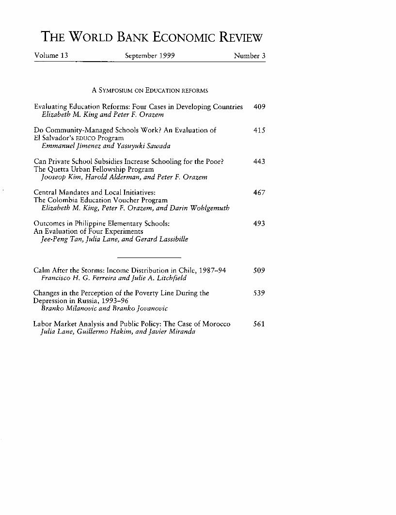
THE WORLD BANK ECONOMIC REVIEWVolume 13 September 1999 Number 3
A SYMPOSIUM ON EDUCATION REFORMS
Evaluating Education Reforms: Four Cases in Developing Countries 409Elizabeth M. King and Peter F. Orazem
Do Community-Managed Schools Work? An Evaluation of 415El Salvador's EDUCO Program
Emmanuel Jimenez and Yasuyuki Sawada
Can Private School Subsidies Increase Schooling for the Poor? 443The Quetta Urban Fellowship Program
Jooseop Kim, Harold Alderman, and Peter F. Orazem
Central Mandates and Local Initiatives: 467The Colombia Education Voucher Program
Elizabeth M. King, Peter F. Orazem, and Darin Wohlgemuth
Outcomes in Philippine Elementary Schools: 493An Evaluation of Four Experiments
Jee-Peng Tan, Julia Lane, and Gerard Lassibille
Calm After the Storms: Income Distribution in Chile, 1987-94 509Francisco H. G. Ferreira and Julie A. Litchfield
Changes in the Perception of the Poverty Line During the 539Depression in Russia, 1993-96
Branko Milanovic and Branko Jovanovic
Labor Market Analysis and Public Policy: The Case of Morocco 561Julia Lane, Guillermo Hakim, and Javier Miranda


THE WORLD BANK ECONOMIC REVIEW, VOL. 13, NO. 3: 409-13
Evaluating Education Reforms: Four Cases inDeveloping Countries
Elizabeth M. King and Peter F. Orazem
This symposium features four studies of education reforms and their impact onenrollment and learning. Three are part of a research project funded by the WorldBank's Development Research Group and its Research Support Budget to evalu-ate innovations in the education systems of selected developing countries. Two ofthe articles focus on Latin America, where decentralization reforms have been inplace since the early 1990s. El Salvador has implemented a program that involvescommunity education councils in the operation of public schools, and Colombiaran a voucher program that subsidized poor students, enabling them to attendprivate secondary schools. The third article analyzes a government subsidy pro-gram in Pakistan that encourages communities to establish nongovernmentalschools that enroll girls. The symposium's fourth study evaluates a pilot projectin the Philippines that uses different school inputs to improve student enrollmentand performance in primary school.
Together, these four studies make an important point for development: byevaluating ongoing policies and programs, policymakers can learn what worksand what does not work under specific circumstances. Learning requires someplanning on the part of program managers and policymakers. It involves system-atically collecting and analyzing information on communities, schools, andstudents, so as to identify changes in outcomes that can be attributed to theprogram.
In most developing countries the central government provides basic educa-tion. The frequently cited reasons for central control are that the technical exper-tise to establish and enforce educational standards, to plan and manage budgets,and to hire and train teachers is not broadly available. Further, local capacity tofinance and operate schools is uneven across communities. Central funding, withcentralized management and centralized norms, is believed to ensure better qual-ity education and more equal access to education. Yet centralized managementhas its own blind spots: learning occurs behind classrbom doors and away fromthe direct gaze of government officials. Consequently, at the risk of losing someof the advantages of centralized control, a growing number of countries have
Elizabeth M. King is with the Development Research Group at the World Bank, and Peter F. Orazem iswith the Department of Economics at Iowa State University. Their e-mail addresses are [email protected] [email protected].
©) 1999 The International Bank for Reconstruction and Development/THE WORLD BANK
409

410 THE WORLD BANK ECONOMIC REVIEW, VOL. 13, NO. 3
been experimenting with ways to transfer responsibility and authority away fromthe center. Fiske (1996:v) describes this movement as a global phenomenon:
Nations as large as India and as tiny as Burkina Faso are doing it. Decen-tralization has been fostered by democratic governments in Australia andSpain and by an autocratic military regime in Argentina. It takes formsranging from elected school boards in Chicago to school clusters in Cambo-dia to vouchers in Chile.
One type of decentralization reform is school autonomy reform, which shiftsmanagement responsibility and resources directly to the school. The hope is thatbringing decisionmaking power and accountability closer to those who teachand manage schools will make schools more efficient in allocating and usingresources and more effective in instructing students. The hope is also that makingthose who teach and manage schools more directly accountable to students, par-ents, and communities will, in turn, establish local incentives that reduce theneed for centralized control and supervision. The reform must change the rela-tionships among the actors in the education system-government officials, schoolprincipals, teachers, parents, and even students-and must affect what teachersdo in the classroom.
El Salvador's Community-Managed Schools Program (Educaci6n con Parti-cipaci6n de la Comunidad, EDUCO) has been expanding education in rural areasby enlisting and financing community management teams to operate schools.These teams are made up of parents, who are elected by the community. They arerequired to follow a centrally mandated curriculum and maintain a minimumstudent enrollment, but they have the power to hire and fire teachers and toequip and maintain the schools. In this issue Jimenez and Sawada examine theimpact of this program on several educational outcomes. They find that, com-pared with traditionally managed schools, EDUCO schools have lower teacher andstudent absenteeism and comparable student achievement, holding the charac-teristics of students constant.
When publicly funded schools rely on nongovernmental management or whenprivate schools receive public funding, the separation between public and privateeducation becomes blurred. Increasingly, governments are relying on partner-ships with the private sector to meet educational needs for which governmentresources alone are inadequate. Private schools already enroll a large number ofstudents in many developing countries, often with the assistance of governmentsubsidies. Governments have pushed private schools to increase their capacity inseveral ways-by paying for construction but relying on private groups to buildand manage private schools (as in the Philippines), by subsidizing part of theconstruction and maintenance costs of private schools and assigning some publicschool teachers to teach in private schools (as in Indonesia), by financing a largeproportion of the salaries of private school teachers (as in Bangladesh), by pro-viding tax incentives to private education foundations (as in Colombia and the

King and Orazem 411
Philippines), and by establishing a student voucher scheme (as in Chile andColombia).
If the government wants to induce private schools to locate in areas that havefew schools, directly funding communities, nongovernmental organizations, oreducation foundations to build schools that will be privately managed may bemore effective than indirectly funding schools through student vouchers. Howprivate schools and communities respond to these incentives depends on the elas-ticity of school supply in the target area. The more elastic is the private supply ofeducational services, the more attractive is it for the government to expand edu-cational services by subsidizing private schools. To our knowledge, no one hasestimated such elasticities. However, supply seems to be more elastic in urbanareas than in rural areas, implying that a larger government subsidy is needed toinduce private investment in rural areas than in urban areas. Even so, unless.theelasticity is zero, private school subsidies represent a potential strategy for ex-panding school capacity.
In the city of Quetta in Balochistan, Pakistan, the government has initiated apilot project that subsidizes the establishment of private girls' schools. Parents inten neighborhoods were given the financial resources and technical assistance tocontract a school operator to open aprivate school in their neighborhood. Theamount of financial resources available was tied to the number of girls that thenew school could attract. This financial assistance proved to be much less thanthe cost of opening and operating a government school in the area. In their analy-sis of this program Kim, Alderman, and Orazem find that all ten neighborhoodsattracted bids from school operators and that the enrollment of both girls andboys rose significantly in response to the creation of the new private schools. Thesuccess of this program bodes well for expanding primary schooling by directlysubsidizing private schools.
Several countries have been experimenting with voucher programs, which trans-fer resources directly to parents to help pay private school tuition. The pro-voucherliterature argues that since school resources are tied to parental demand, whichpresumably responds to school quality, voucher programs force public and pri-vate schools to provide quality education efficiently. Schools that offer poor-quality education or use resources inefficiently will have to improve or face bank-ruptcy. Opponents of voucher programs dispute the efficiency and quality claims,suggesting that vouchers further segregate access to schools by wealth. To date,there is limited empirical evidence to guide the debate over which view is correct.
For developing countries the efficiency concerns may be secondary to the morebasic problem. that demand for schooling exceeds supply. When poor studentsare prevented from continuing in school because of overcrowded public schoolsor the lack of schools, the private sector may offer a way to expand school capac-ity. Vouchers can be targeted to the poor to prevent benefits from leaking to thewealthy and to induce private schools to locate or expand in areas that cater tothe poor. In this issue King, Orazem, and Wohlgemuth examine how schools andmunicipalities responded to Colombia's national voucher system. They demon-
412 THE WORLD BANK ECONOMIC REVIEW, VOL. 13, NO. 3
strate that municipalities were more likely to participate if excess demand forschooling was present but modest and if local private schools already had thecapacity to absorb additional students. The schools that accepted voucher stu-dents tended to have fees and average student test scores that were in the lowerrange among private schools, although the design of the voucher program mayhave prevented the lowest-price and lowest-quality schools from participating.Most important, the targeted vouchers appear to have increased secondary schoolenrollment among poor children, allowing very little leakage to rich householdsor to schools catering to the wealthy.
Although many countries are reforming their education systems, few are sys-tematically evaluating the impact of those reforms. This is the case in both indus-trial and developing countries. Yet impact evaluations are powerful tools forpolicymakers. They provide the information needed to terminate or improve in-effective policies or programs. And this information may be especially importantfor evaluating innovative reforms or programs that do not have well-chartedhistories.
Often the impact of a specific reform or program cannot be isolated from theimpact of coincident changes in the policy or economic environment. We canmeasure the impact if we know how the participants (or treatment population)would have fared without the program. This is the counterfactual state, and theselection and observation of appropriate control populations to characterize thisstate are important features of evaluation strategies.
The Philippine study demonstrates the benefits of monitoring and evaluatingeducation programs when the use of randomized control designs is feasible. Inthe Philippines the central government continues to play a key role in supplyingprimary education, as decentralization has not yet progressed to the extent that ithas in the other countries. This article illustrates that even within the public sec-tor, the government can benefit from routine monitoring and evaluation activi-ties. Tan, Lane, and Lassibille examine four experimental interventions in se-lected low-income areas, using pre- and post-intervention data collected fromprogram and control schools. The authors find that providing teachers with learn-ing materials and encouraging parents to get more involved in the schooling oftheir children were more effective than a school feeding program in reducingdropout rates and increasing learning.
The four articles in this symposium illustrate that it is not always easy, how-ever, to determine whether or not a particular policy or program has attained itsobjectives. The authors apply a variety of impact evaluation strategies dependingon the nature of the reform, the stage at which the evaluation began, and theavailability of appropriate data. Although developing an evaluation strategy atthe inception of the reform or program makes evaluation a little easier, doingso is often not possible. In the absence of baseline surveys, evaluations may haveto rely on more advanced statistical methods that may be more difficult fornonstatisticians to understand and undertake.

King and Orazem 413
The ability to rank interventions is a valuable policy tool, as countries searchfor effective strategies to improve schooling outcomes within constrained educa-tion budgets. For the World Bank the practice of evaluating the most innovativecomponents of its investment projects both improves the quality of its portfolioand enriches the knowledge base that it can share with its member countries.
REFERENCES
Fiske, Edward. 1996. Decentralization of Education: Politics and Consensus. Washing-ton D.C.: World Bank.


THE WORLD BANK ECONOMIC REVIEW, VOL. 13, NO. 3: 415-41
Do Community-Managed Schools Work? AnEvaluation of El Salvador's EDUCO Program
Emmanuel Jimenez and Yasuyuki Sawada
This article examines how decentralizing educational responsibility to communities andschools affects student outcomes. It uses the example of El Salvador's Community-Managed Schools Program (Educaci6n con Participaci6n de la Comunidad, EDUCO),
which was designed to expand rural education rapidly following El Salvador's civil war.Achievement on standardized tests and attendance are compared for students in EDUCO
schools and students in traditional schools. The analysis controls for student character-istics, school and classroom inputs, and endogeneity, using the proportion of EDUCO
schools and traditional schools in a municipality as identifying instrumental variables.The article finds that enhanced community and parental involvement in EDUCO schoolshas improved students' language skills and diminished student absences, which mayhave long-term effects on achievement.
Central governments in developing countries usually play a major role in allocat-ing educational resources. Even when authority is delegated to subnational lev-els, such as provinces or municipalities, individual school administrators andparents play only a limited part. This kind of centralized structure may work bestfor regulating and administering large systems uniformly, but it may also be in-effective and expensive when school needs differ widely across communities andwhen there are diseconomies of scale. Moreover, a centralized system can stiflethe initiative of those who are most critical in affecting school outcomes-teachers, principals, and parents.
Despite the compelling case for school-based management, there is relativelylittle empirical evidence documenting its merits in developing countries.' Themain reason is that these administrative arrangements have only recently been
1. Two exceptions are James, King, and Suryadi (1996) for Indonesia, and Jimenez and Paqueo (1996)for the Philippines. Both studies conclude that community-based involvement improves efficiency.
Emmanuel Jimenez is with the Development Research Group at the World Bank, and Yasuyuki Sawadais with the Department of Advanced Social and International Studies at the University of Tokyo. Their e-mail addresses are [email protected] and [email protected]. This project has beenfinancially supported by the Development Research Group and the Research Support Budget (RPo 679-18and 682-08) of the World Bank. The authors gratefully acknowledge the comments and support from theEvaluation Unit of the Ministry of Education of El Salvador, which collected the data. They also thankMarcel Fafchamps, Paul Glewwe, Elizabeth King, Takashi Kurosaki, Martin Ravallion, Laura Rawlings,Fernando Reimers, Diane Steele, the anonymous referees and editors, and participants in seminars at theWorld Bank, Stanford University, the University of the Philippines, International Child Development Centre(United Nation's Children's Fund, Florence), and the Institute of Developing Economies Uapan) for usefuldiscussions and comments.
© 1999 The International Bank for Reconstruction and Development/THE WORLD BANK
415

416 THE WORLD BANK ECONOMIC REVIEW, VOL. 13, NO. 3
implemented (World Bank 1994, 1995, 1996). One celebrated example is ElSalvador's Community-Managed Schools Program (Educaci6n con Participaci6nde la Comunidad, EDUCO). EDUCO is an innovative program for both preprimaryand primary school designed to decentralize education by strengthening the di-rect involvement and participation of parents and community groups.
A prototype of today's EDUCO schools emerged in the 1980s, when public schoolscould not be extended to rural areas because of El Salvador's civil war. Some com-munities took the initiative to organize their own schools, which an association ofhouseholds administered and supported financially. Although these early attemptswere constrained by the low income base in rural areas, they demonstrated com-munities' strong inherent demand for education and desire to participate in thegovernance of their schools. In 1991 El Salvador's Ministry of Education (MINED),
supported by aid agencies such as the World Bank, decided to use the prototypethat communities themselves had developed as the basis of the EDUCO program.
Today, EDUCO schools are managed autonomously by community educationassociations (asociaciones comunales para la educaci6n, ACEs), whose electedmembers are parents of the students. Reimers (1997) describes community asso-ciations as being composed of literate members of the community who are givenbasic training in school management. These associations meet periodically withteachers and also provide them with teaching materials. In EDUCO schools theACEs are in charge of administration and management; MINED contracts them todeliver a given curriculum to an agreed number of students. The ACES are thenresponsible for hiring (and firing) teachers, closely monitoring teachers' perfor-mance, and equipping and maintaining the schools. The partnership betweenMINED and the ACES is expected to improve school administration and manage-ment in that the ACES can better gauge local demand. In the future MINED intendsto introduce community management to all traditional schools.
The EDUCO program was conceived as a way to expand educational access quicklyto remote rural areas. Initial evidence indicates that it has accomplished this goal(El Salvador, MINED 1995; Reimers 1997). The question that remains is whetherthis expansion has come at the expense of learning. Professional administrators inthe center are less involved in the day-to-day running of schools, which are now inthe hands of local communities. But many of the parents in these communities havean inadequate education themselves. Thus it remains to be seen whether movingaway from traditional, centralized programs and toward greater community andparental involvement also improves students' learning.
This article assesses the impact of EDUCO schools. We estimate school produc-tion functions using three measures of educational outcomes for third-grade stu-dents.2 Two of the measures are standardized test scores in mathematics and
2. This study is part of a larger effort by the World Bank to distill the lessons of decentralized education(see World Bank 1996). Eventually, we want to determine whether all students in EDUCO schools achievebetter educational outcomes at comparable costs relative to their counterparts in traditional public schools.This article has a more limited objective: it uses school production functions to compare three measures ofeducational outcomes among third-grade students only.

Jimenez and Sawada 417
language. These may be good indicators of educational outcomes. However, theymay also be relatively unresponsive in the short run to changes in school gover-nance. Thus we also use an indicator that can be considered more of an interven-ing variable in determining student achievement but is likely to exhibit a short-run response: the number of school days that a student has missed.
As with all comparisons of educational achievement, the key is to quantifyhow much of the differential in academic achievement can be explained by differ-ences in household background, the schools' quantitative inputs, and, most im-portant, organizational factors attributable to intangible differences in the waythat traditional and decentralized schools are run.3 We also address parents' en-dogenous school choice by explicitly considering how the government selectedwhich municipalities would be the first to have EDUCO schools.
I. THE CONCEPTUAL AND EMPIRICAL FRAMEWORK
Educational outcomes are products of the complex interactions of agents whoparticipate in the schooling process. Students' characteristics and motivation arekey, but so are the actions of individual parents, parent groups (such as parent-teacher associations), teachers, and administrators from the school level up tothe education ministry. In addition, agents not directly connected to the educa-tional system can affect educational outcomes if they influence the environmentin which students learn. For example, decisions about road infrastructure in alocality could afford access to certain types of schools, or the provision of elec-tricity in a municipality could enable students to study at night.
The Basic Model
It would be impossible to model the structural relationships that capture thebehavior of each relevant agent.4 Instead, we postulate a simple reduced-formmodel of educational outcomes (Y). Most studies measure educational output byusing students' achievement scores, attendance rates, repetition rates, decision tocontinue in school, or dropout rates. These variables are thought to capture pros-pects of future earnings in the labor market. In this article we focus on two com-ponents of Y: scores on standardized achievement tests (S) and days absent fromschool (A).
Studies of education production functions have had mixed success in explain-ing S.5 Aside from measurement and estimation issues, outcomes may be deter-mined by endogenous choices. For example, some of the explanatory policy vari-ables that determine S, such as type of school, may be systematically related tounobservable characteristics, which themselves may not be random across obser-vations. This could lead to bias. As explained below, we attempt to correct for
3. See Levin (1997) for a good review of these intangibles.4. McMillan (1999) presents an interesting model of the interaction of parental and school preferences
in determining educational outcomes.5. See Hanushek (1995) for a review.

418 THE WORLD BANK ECONOMIC REVIEW, VOL 13, NO 3
this problem by modeling and estimating the choice of school type and thenusing that estimate in the production function to control for participation. It isoften difficult to identify such models. But we are able to use the participationrule that the Salvadoran authorities used in choosing where to place EDUCO schoolsas the identifying restriction that directly affects choice but not outcomes.
It may take time for a policy change such as decentralization to affect schoolperformance, which tends to be a cumulative measure. We thus also consider animportant intervening variable that eventually influences student outcomes: ab-sence from school (A). Students may be absent for a number of reasons, some ofwhich, such as illness, have nothing to do with decentralization. But other rea-sons may be tied to school organization and management. Students (or theirparents) may not be motivated to ensure regular attendance because the qualityof schooling is poor or because parents do not feel involved in the educationprocess. Also contributing to student absence is teacher absence, an importantreason why students do not attend school in El Salvador. If teachers are absent,classes are usually canceled, since there is no tradition of using substitute teach-ers. Although teachers are sometimes absent for legitimate reasons, such as sick-ness, more often they are simply not fulfilling their duty. Teacher absence is anissue in many countries besides El Salvador:
Lack of motivation and professional commitment produce poor attendanceand unprofessional attitudes towards students. Teacher absenteeism andtardiness are prevalent in many developing countries . . . absenteeism isespecially acute in rural areas. Students obviously cannot learn from a teacherwho is not present, and absenteeism among teachers encourages similarbehavior among students. In some countries . . . parents react to high ratesof teacher absenteeism by refusing to enroll their children in school.(Lockheed and Vespoor 1991: 101.)
Teacher absence could be minimized if teachers were appropriately monitored.We would expect that, in a decentralized school, parental involvement wouldmitigate such behavior.
We assume that the components of Y = [S A] can be independently estimated.A will likely affect S, and we assume an implicit recursive process S = S(A), inwhich the residuals from the different equations are independent of each other,and the matrix of coefficients of endogenous variables is triangular. Each struc-tural equation can thus be estimated by ordinary least squares (OLS), equation byequation (Greene 1997).
A simple model for the ith student in the nth school in the mth community is
(1) Y'jn = f(X,,, ... , Cm ,..t.)
where X is a vector of student and household characteristics, C is a vector ofcommunity variables for municipality m, and D is the type of school, either adecentralized EDUCO school or a traditional school. In this model the type ofschool is assumed to determine most of the school characteristics that affect stu-
Jimenez and Sawada 419
dent outcomes. This model is the ultimate reduced form-it assumes that theeffect that a school's observed characteristics, such as class size and teacher char-acteristics, have on achievement is fully determined by the school's managementstructure (that is, whether it is a decentralized EDUCO school or a traditionalschool) and the characteristics of the students and parents who participate indecisions concerning the school.
We can often observe the effects of management structure through differencesin school and classroom inputs, such as teacher-pupil ratios, teacher remunera-tion, or the educational background of teachers and administrators. But even ifwe were to enter as many observable school characteristics as we could in equa-tion 1, the type of school may still be significant because it captures unobservedmanagerial inputs (Levin 1997). Indeed, in reviewing 96- studies on the effects offive educational inputs on student performance in developing countries, Hanushek(1995) concludes that there are no clear and robust technical relationships be-tween key school inputs and student performance.6 Thus differences in resourcesmight not be important determinants of school outputs, implying that schools indeveloping countries are paying for inputs that have little consistent effect onstudent performance. We distinguish the unobserved effect of community par-ticipation from the other unobserved effects of management by explicitly takinginto account differences in the level of community involvement. Accordingly, wealso derive an alternative model:
(2) Yi,,m = f(X)m,J Cm, Di..m. Zflfli PJ-nm)
where Z is a vector of observed school and classroom characteristics, and P is theintensity of community participation. Since Z and P vary by school rather thanby student, equation 2 expresses the achievement of the ith student in the nthschool. To simplify notation, we drop the school and community subscripts inthe rest of this article.
Empirical Specification
Linearizing and adding a stochastic term, which represents a well-behavedmeasurement error term, to equation 1, we derive the following regressionformula:
(3) Y, = X,+ C+ D,a + u, .
D takes a value of 1 if the ith student attends a decentralized EDUCO school and 0if the student attends a traditional, centralized school. By assumption, E(u,) = 0and Var(u,) = 02. We add school and classroom characteristics and the intensityof community participation to derive the empirical version of equation 2.7
6. Hanushek (1995) does, however, suggest that a minimal level of basic school resources, such astextbooks and facilities, is important to student achievement.
7. To simplify notation, we do not add the error terms associated with the school and municipal-levelvariables. We handle the school variables by using a program participation model and the municipal-levelvariables by using a municipality-level fixed-effects model.

420 THE WORLD BANK ECONOMIC REVIEW, VOL. 13, NO. 3
Observed household and student characteristics reflect the ability of parentsto provide a supportive environment for their children. If capital markets wereperfect, then life-cycle consumption and human capital investments could bedetermined independently. Parents would simply borrow to finance the homeinputs needed to maximize their children's learning. But since credit markets arefar from perfect in El Salvador, the economic circumstances of the householdbecome important. In this article we use asset variables to control for the at-tributes that are hypothesized to be positively correlated with schooling out-comes (homeownership and the availability of electricity, sanitary services, andpiped water). In addition, we control for parents' education, which may alsodirectly affect living standards and preferences for children's education.
We cannot measure students' innate ability directly. However, student charac-teristics that may be important include gender, since parents or teachers my treatboys and girls differently; age, since older students, while more mature and morelikely to score higher, may be self-selected as underachievers and left behind bytheir cohort; and number of siblings, since the greater the number, the less timeparents have to devote to any one child, that is, there are resource competitioneffects.
We capture community characteristics, C, by municipality-level fixed effects.In El Salvador municipalities are the next administrative level below the depart-ment level. There is substantial variance in the distribution of resources acrossmunicipalities, which could affect students' access to ancillary services, such asthe availability of electricity needed to study, which, in turn, could affect school-ing outcomes.
Endogenous Program Participation
A key. estimation issue is endogenous program participation. Endogeneity mayarise because parents choose which type of school their children attend (condi-tional on their choosing to send them to school, since we do not have informa-tion on children who are not in school).8 If attendance at an EDUCO school issystematically based on unobserved characteristics that could also influence stu-dent achievement, then the OLS estimates of the effect of EDUCO would be biased.That is, oa in equation 3 may not accurately measure the value of attending anEDUCO school.
The direction of the bias is ambiguous. If the important unobserved character-istics are students' motivation to learn and parents' commitment to education,and these variables are positively correlated with participation in EDUCO, thencomparing outcomes, even after holding constant for observed characteristics,
8. Although EDUCO schools were targeted to areas with limited primary school coverage, parents wouldstill have had a choice of whether or not to send their children to school. They could have had theirchildren commute, albeit over long distances (child fosterage for schooling is not uncommon in developingcountries; see Ainsworth 1992 and Glewwe and Jacoby 1994). Or, they could have changed residences(Salvadoran migration rates are high). Unfortunately, the school-based nature of the sample prevents usfrom including nonattendance as an option.

Jimenez and Sawada 421
would overestimate the effect of EDUCO. This bias, however, may be mitigated bythe fact that EDUCO targets economically disadvantaged communities.
To take the possibility of bias into account, we explicitly model program par-ticipation (that is, whether or not a student enrolls in an EDUCO school ratherthan in a traditional school). Using a familiar method for obtaining so-calledtreatment effects, we then estimate this model to obtain the parameters needed tocorrect equation 3.9
WHAT DETERMINES PROGRAM PARTICIIPATION? We assume that governments setpriorities regarding which municipalities will receive an EDUCO school. Householdsthen use that information to choose the type of school that maximizes their indirectlifetime utility, V. Parents make this choice by weighing the benefits and costs ofan EDUCO school relative to other types of schools. The benefits of EDUCO dependon households' perceptions of the virtues of a decentralized program. Some ofthese preferences can be captured by measurable household characteristics, X,but others are unobserved.
The cost of an EDUCO school relative to a traditional school depends on rela-tive direct costs, such as tuition payments, books, and other fees. The most im-portant components of cost are largely the same for both types of schools: allschools and books are free in first through sixth grade. But there are differencesin the other direct costs. EDUCO students do not pay a registration fee, do not buyuniforms, and receive a basic package of school supplies, such as pencils, rulers,and markers. Students in traditional rural schools must bear all of these costs."0
However, EDUCO parents must devote a substantial amount of time to the schoolby providing school meals and by building, maintaining, and administering theschool."
The principal cost differential between EDUCO and traditional schools comesfrom differences in access, given the relative paucity of schools in rural areas. Wedo not have information on households' schooling options (such as the distancefrom households to feasible EDUCO or traditional schools) because our data areschool-based, not household-based. However, we assume that a household ismore likely to choose an EDUCO school if the government considers the munici-pality a priority for the program and thus an EDUCO school is available in thecommunity. The government gives priority to municipalities considered to beneediest according to a classification system developed by MINED and the Minis-try of Health.
Municipalities' uneven access to social services has always been a serious issuein El Salvador. However, poverty is more widespread in smaller municipalities,
9. See Greene (1997: 981-82) for a clear discussion of this estimation strategy.10. We are grateful to Diane Steele of the World Bank for this information, which she received from a
phone interview with MINED staff.11. We do not have data on the magnitudes of these costs. We assume in this article that these cost
differentials are roughly offsetting for decentralized and traditional schools. We will verify this assumptionwith data from surveys that were fielded only in 1999.

422 THE WORLD BANK ECONOMIC REVIEW, VOL. 13, NO 3
which usually lack the financial and institutional capacity to administer andmanage social services. The EDUCO program was developed in 78 of the country'spoorest municipalities. It started in 1991 with six ACES in three departments; bythe end of 1992, the program had extended to all 14 departments.
The key variables in the targeting system are the incidence of severe malnutri-tion (the percentage of undersize children in the municipality), the repetition rate,the percentage of overage students, and the net enrollment rate. Higher valuesfor the first three variables, and a lower value for the last, make a municipality ahigher priority. In the next section we discuss how this prioritization affects ourchoice of instruments.
THE FORMAL MODEL OF PROGRAM PARTICIPATION. In the model a householdchooses the type of school that yields the highest level of indirect utility, VJ.'2
There are two options: j = D if the household chooses a decentralized EDUCO
school or j = T if the household chooses a traditional rural school. V, depends onthe relative benefits and costs of attending an EDUCO school as perceived by parents.Parents choose EDUCO if, for the ith student:
(4) D,* = VDj- VTj > °
where D* is a latent variable that describes the likelihood that a child is in anEDUCO school. It is determined by:
(5) 'Di*=Wi.+E,
D, = 1 if Di* > 0; 0 otherwise.
In equation 5, E(s,) = 0, Var(E,) = Cy2J 0) = [3 'ir']', and W; = [X, R,j, which is avector capturing the benefits and costs of attending an EDUCO school. These ben-efits and costs are proxied by household characteristics and R, a vector of schooldensity variables (the percentages of EDUCO and traditional schools in all primaryschools in a municipality). Equation 5 can be estimated as a probit model underthe assumption that £, is normally distributed.
The essence of the endogenous participation problem is that the errors in equa-tions 3 and 5 are correlated, that is, Cov(ui, E,)X 0, leading to bias.'3 If we assumethat u, and £; are jointly normally distributed, the expected value of the outcomevariable for EDUCO and traditional schools would be:
(6) E(YiID, = 1) = Xij3 + CmY+ X+ouFkDi
(7) E(Y,I D, = 0) = X,, + Cmy -O-T,
12. The basic structure of the model follows the standard treatment of program participation (Greene1997: 981-82). It is also closely related to the econometric model of self-selection (Willis and Rosen 1979and Cox andJimenez 1991). Readers who are not interested in the technical discussion of EDuco participationcan proceed to the next section.
13. Note that E(u, l D,* > 0) = E(u, l W, o- + E, > 0) • 0.

Jimenez and Sawada 423
where XD, and XT, are selection terms estimated from Mills ratios.14 The differencein expected performance between EDUCO participants and nonparticipants, con-ditional on having chosen a type of school, can be obtained by subtracting equa-tion 7 from equation 6:
(8) E(Y, I D, = 1) - E(Y, I Di = O) =a + CF (XD, + XT,)
where cx is the coefficient of the EDUCO intercept and is usually referred to as the"true" program effect (see Maddala 1983).
Thus if we define e, = u, - (7OuXD, D, + au,XTi (1 - Di), a term whose expectationis O for each of the cases D = (1, 0), the following regression would yield unbiasedestimators:
(9) Yi = XP + C, y + D, a + CU [D, Di -XT, (1 -D,)i] + e,.
If we omitted the selection correction terms (in brackets) from this regression, thedifference in equation 8 would be equal to what is usually estimated as the leastsquares coefficient on the treatment dummy variable. But this expression wouldoverestimate or underestimate the treatment effect, depending on the direction ofthe participation bias.
To estimate this model, we employ a two-step method.'5 In the first step weestimate equation 5 as a probit model and then use the results to calculate theinverse Mills ratios XD and XT. In the second step we use the estimated inverseMills ratios to form the participation terms in equation 9. We then estimate equa-tion 9 with municipal dummies to capture regional fixed effects.
If the error terms in the probit and outcome equations are negatively corre-lated, that is, if Y,, < 0 (this would occur if an unobserved variable, such asstudent motivation, negatively affected the likelihood of attending an EDUCO schoolbut positively affected student achievement), then equation 6 implies that thepredicted score of a student drawn randomly from the population would be un-derestimated in the case of EDUCO schools if we use sample mean scores. This canbe easily verified by the relationship, E(Yi I D, = 1) < X,f3 + C,,,y + ax if 4%, < 0. Asimilar calculation can be done for equation 7 in the case of traditional schools.
In a linear model, estimation and parameter identification are possible only ifthe vectors [X Cm] and W have no elements in common and are linearly indepen-dent. However, in the model above, even if [X C,,,] and W are identical, equation9 is estimable. This is because the first-stage estimation results are entered as anonlinear function in the second stage (equation 9). The nonlinearity helps toidentify the model.
14. Assuming joint normality between u, and e,, E(u,l Wc+e,>0) =E(u,lD* >0)= au,, whereXD = O(W, t)/ 4)(W.()), the inverse Mills ratio. Similarly, E(u, I D* <0) = E(u, IW, o+e,<0) •0, which wecan rewrite as E(u, I D* < 0) = - oXT, where T, = 4(W, w) / [ 1 - (D(W w)]
15. An alternative way to estimate program participation on unobservables is to use a maximumlikelihood method without focusing on Mills ratios. However, this method is more burdensomecomputationally.

424 THE WORLD BANK ECONOMIC REVIEW, VOL. 13, NO. 3
II. DATA DESCRIPTION
MINED collected the data in October 1996 with the assistance of the WorldBank and the U.S. Agency for International Development (USAID). The surveycovered 162 of the country's 262 municipalities. These municipalities share re-sponsibility with the central government for delivering social services.
Since EDUCO was introduced only in 1991, it was not possible to compare thescores on achievement tests given in 1996-only five years later-of EDUCO stu-dents who were about to finish their primary education and students in tradi-tional schools. Instead, MINED decided to compare outcomes for third graders.MINED designed the sampling scheme so that the survey was nationally represen-tative. Moreover, the sample was selected so as to consider four types of schools:pure EDUCO, pure traditional, mixed, and private. We dropped students fromprivate schools and traditional public urban schools from the sample, since theyare not comparable to EDUCO students. Mixed schools have both EDUCO sectionsrun by ACES and traditional sections. Some EDUCO programs rented space fromtraditional schools. The small number of students in these mixed schools attendeither EDUCO or non-EDUCO classes located in traditional schools. Since the ad-ministration and management of mixed schools are different from the adminis-tration and management of pure EDUCO and traditional schools, and thus weshould control for unknown management and school-level cross-effects, we couldnot include mixed schools in pure school samples. Nor could we isolate them asa separate category because of the small sample size. To ensure the robustness ofour results, we based our estimations on pure schools only.16 This left us with605 students in 30 EDUCO schools and 101 traditional schools.
The survey comprises five questionnaires, one each for students, parents, schooldirectors, teachers, and parent associations. The students' questionnaire requestsinformation about students' relationship with their guardians, type of school,gender, and achievement test results. The parents' data include information onfamily background and living standards, such as parents' education level, thehousehold's living standard, and asset ownership, as well as detailed socioeco-nomic information on students, including age, schooling, and health status. Thequestionnaire for the school director consists of questions about the director,student enrollment, the quality and quantity of teachers, school facilities, andfinances. The data collected from teachers include their educational background,years of experience, and salaries, as well as information about the -classroom,such as the availability of school materials and frequency with which members ofthe community association visit the classroom. Lastly, the community and par-ent association questionnaire contains qualitative information on how the asso-ciation is organized and how members participate in administration and man-agement of the school. The information on EDUCO schools was collected from
16. The results with both mixed and pure samples, which are not reported here, are consistent with theresults for pure schools only.
Jimenez and Sawada 425
ACES, and the information on traditional schools was collected from a counter-part parent organization, the Sociedad de Padres de Familia.
Dependent Variables
MINED administered the achievement tests in October 1996 with the assistanceof the Intercultural Center for Research in Education (El Salvador, MINED 1997).The tests were given nationally in the third, fourth, and sixth grades, but becauseEDUCO students had reached only the third grade when the data were collected,we use only the third-grade results in the analysis. Also, we focus only on scoresfor the mathematics and language tests, ignoring the social studies, science, health,and environment components.
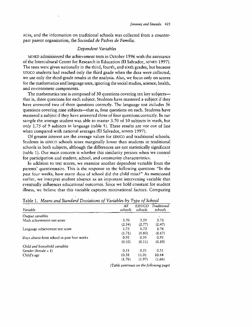
The mathematics test is composed of 30 questions covering ten key subjects-that is, three questions for each subject. Students have mastered a subject if theyhave answered two of three questions correctly. The language test includes 36questions covering nine subjects-that is, four questions on each. Students havemastered a subject if they have answered three of four questions correctly. In oursample the average student was able to master 3.70 of 10 subjects in math, butonly 1.75 of 9 subjects in language (table 1). These results are not out of linewhen compared with national averages (El Salvador, MINED 1997).
Of greater interest are the average values for EDUCO and traditional schools.Students in EDUCO schools score marginally lower than students in traditionalschools in both subjects, although the differences are not statistically significant(table 1). Our main concern is whether this similarity persists when we controlfor participation and student, school, and community characteristics.
In addition to test scores, we examine another dependent variable from theparents' questionnaire. This is the response to the following question: "In thepast four weeks, how many days of school did the child miss?" As mentionedearlier, we interpret student absence as an important intervening variable thateventually influences educational outcomes. Since we hold constant for studentillness, we believe that this variable captures motivational factors. Comparing
Table 1. Means and Standard Deviations of Variables by Type of SchoolAll EDUCO Traditional
Variable schools schools schools
Output variablesMath achievement test score 3.70 3.59 3.73
(2.54) (2.77) (2.47)Language achievement test score 1.75 1.73 1.76
(1.71) (1.85) (1.67)Days absent from school in past four weeks 0.95 0.95 0.95
(0.10) (0.11) (0.10)Child and household variablesGender (female = 1) 0.51 0.51 0.51Child's age 10.58 11.01 10.44
(1.76) (1.97) (1.66)
(Table continues on the following page)

426 THE WORLD BANK ECONOMIC REVIEW, VOL. 13, NO. 3
Table 1 (continued)All EDUCO Traditional
Variable schools schools schoolsChild lives without parent(s)" 0.14 0.16 0.13Child had respiratory illness or flu in the past two weeksa 0.60 0.63 0.59Number of siblings (ages 4-15) 2.01 2.11 1.98
(1.54) (1.50) (1.56)Mother began basic education' 0.53 0.50 0.54Mother's education missing3 0.08 0.06 0.09Father began basic educationa 0.39 0.38 0.40Father's education missinga 0.04 0.03 0.04Own housea 0.72 0.68 0.73Electricity availablea 0.58 0.28 0.67Sanitary service availablea 0.18 0.06 0.22Water availablea 0.06 0.01 0.08
School variablesTeacher-pupil ratio (school level) 0.04 0.05 0.03
(0.056) (0.09) (0.041)Sanitation or latrine available at school, 0.93 0.89 0.94Electricity available at schoola 0.68 0.30 0.80Piped water available at schoola 0.32 0.12 0.38
Teacher and classroonm variablesTeacher finished university education" 0.46 0.75 0.37Years of teacher experience 7.83 4.37 8.89
(6.44) (2.71) (6.87)Monthly base salary of teacher (thousands of colones) 3,035.21 2,919.23 3,070.71
(523.38) (269.40) (574.84)Teacher receives bonusa 0.64 0.74 0.61All students have math textbooka 0.61 0.58 0.62Math textbook information missing" 0.11 0.25 0.07All students have language textbooka 0.59 0.59 0.59Language textbook information missinga 0.12 0.28 0.07Teacher instructs multigrade classrooma 0.24 0.39 0.20Multigrade information missing' 0.01 0.04 0.00Number of books in classroom library 74.32 114.63 61.98
(197.59) (272.84) (166.42)Classroom library information missing, 0.47 0.24 0.54
Comniunity participation variableNumber of parent association visits to classroom in
the past month 2.52 5.65 1.56(4.82) (6.59) (3.63)
Regional school distributionPercentage of pure EDUCO schools in all primary schools
within municipality 0.21 0.75 0.04(0.34) (0.29) (0.11)
Percentage of pure traditional schools in all primary schoolswithin municipality 0.69 0.15 0.86
(0.37) (0.28) (0.20)Inverse Mills ratio 0.00 0.24 0.07
(0.33) (0.47) (0.22)Number of observations 605 142 463
Note: Standard deviations are in parentheses.a. Binary variable equals 1 if response is "yes," 0 otherwise.

jin2enez and Satvada 427
sample means themselves indicates that, on average, students in both EDUCO andtraditional schools missed 0.95 days in the four weeks before the survey.
Explanatory Variables
The means of the explanatory variables show the following. Both EDUCO andtraditional schools have an equal number of girls and boys. A fairly large portionof students live without their parents, the proportion being slightly higher forEDUCO students. EDUCO students also have more siblings and are older, althoughthe differences are not significant.
Parents of traditional school students have more education than parents ofEDUCO students. Fifty-four percent of mothers or female guardians of traditionalstudents have had some basic education compared with 50 percent for EDUCO
students. The gap also holds for fathers (40 and 38 percent). These differences ineducation are reflected in the asset variables. Fewer EDUCO parents are homeownersor have access to electricity, sanitary services, and running water, suggesting thatEDUCO students come from poorer backgrounds than traditional school students.
The socioeconomic characteristics of students are consistent with the charac-teristics of schools. While teacher-pupil ratios, access to textbooks, and the avail-ability of sanitary facilities are similar in both types of school, fewer EDUCO schoolshave access to electricity or piped water. However, more EDUCO teachers havefinished university education, although they have less teaching experience. TheEDUCO teaching corps consists of relatively young recent graduates who receive abonus for teaching in the program. Another difference is that EDUCO parent asso-ciations visit classrooms more than once a week, which is three to four timesmore often than their traditional counterparts.
The overall picture, then, is one of poor communities that have succeeded inmobilizing parents to become more involved in their children's education, de-spite their lower standard of living. What we want to know is how much of thedifferences in outcomes are due to EDUCO.
Identification
We account for possible program endogeneity by explicitly modeling the like-lihood of participation in EDUCO and using that information to correct the pro-duction function. The main challenge with such corrections is specifying the iden-tifying restriction that allows us to estimate the model.
We include the percentages of EDUCO and traditional schools in all primaryschools in each municipality to capture the relative cost of access to each type ofschool. Arguably, these percentages affect the likelihood that a student will at-tend an EDUCO school without directly affecting the education production func-tions at the student level. To isolate general community effects on achievementfrom the cost-of-access effect, we also include municipal fixed effects in the edu-cational output equation (equation 3). Although the percentages of EDUCO schoolsare linear combinations of these municipal.dummies, we achieve identificationbecause the probit participation equation has a nonlinear functional form.

428 THE WORLD BANK ECONOMIC REVIEW, VOL. 13, NO. 3
In order to test the robustness of our results, we also estimate specificationsthat do not rely exclusively on functional form for identification. For example,instead of using the proportion of EDUCO schools in each municipality, we in-clude the variables that the government uses to prioritize program placement: theextent of malnutrition, the proportion of overage students, repetition rates, andnet enrollment rates. Because the government exogenously determines theprioritization formula, the variables included can be used to identify the partici-pation equation. We do not include them in the achievement equations, since, tothe extent that local geographic conditions affect achievement, the municipalfixed effects capture their influence. Because our basic qualitative results do notchange with these specifications, and to conserve space, we do not report theresults here. They are, however, available from the authors.
III. EMPIRICAL RESULTS: STUDENT ACHIEVEMENT
The first step of the analysis is to estimate the determinants of participating inEDUCO to correct for possible endogeneity. The most significant variables aremother's education, household assets, and the geographical variables that cap-ture the cost of EDUCO schools relative to that of traditional schools. Mother'seducation, homeownership, and the availability of water are negatively corre-lated with EDUCO participation (table 2). Students from households that are bet-ter off have a higher likelihood of attending a traditional school. As expected, theavailability of an EDUCO school within each municipality significantly increasesthe probability of enrolling in an EDUCO school.
The next question is whether an EDUCO student (captured by an EDUCO dummyvariable) achieves different test scores than a traditional school student. The re-gressions, which include the participation correction, use math and languageachievement as dependent variables, and student and community characteristics(the latter captured by municipality fixed effects) as explanatory variables (table3). The negative coefficient of the Mills ratio indicates that the error terms of theparticipation and achievement equations are negatively correlated. This meansthat EDUCO students have unobserved characteristics that are negatively corre-lated with achievement test scores.
EDUCO's unconditional effect on language test scores is positive and signifi-cant, while its effect on math performance is positive and not significant (table4). Thus the program has not lessened child learning (after correcting for partici-pation). In fact, it has improved performance in language. However, our measureof EDUCO's advantage in language may be imprecise. The estimate of the EDUCO
coefficient is sensitive to the specification of the participation equation-it be-comes insignificant when we use in the first stage the municipal prioritizationvariables instead of the proportion of EDUCO schools in each municipality."7
17. However, the qualitative results described in the text hold. The results are available from theauthors.

Jimnenez and Sawada 429
Table 2. Probit Analysis of School ChoiceVariable Coefficient
Child and household variablesGender (female = 1) -0.14
(0.54)Child's age 0.11
(1.39)Child lives without parent(s)a 0.05
(0.12)Child had respiratory illness or flu in the past two weeksa -0.47
(1.72)*Number of siblings (ages 4-15) 0.04
(0.43)Mother began basic educationa -0.54
(1.75)*Mother's education missinga -1.29
(2.07)*Father began basic educationa -0.37
(1.18)Father's education missinga -0.48
(0.63)Own house, -0.59
(2.08)**Electricity availablea -0.17
(0.61)Sanitary service availablea 0.19
(0.46)Water availablea -3.00
(1.88)*Regional school distribution (proxies for cost variables)Percentage of pure EDUCO schools in all primary schools within municipality 5.96
(7.14) ***
Percentage of pure traditional schools in all primary schools within municipality -1.66(2.63) -
Constant -1.19(1.11)
Log likelihood -62.42Pseudo R2 0.81
Significant at the 10 percent level.Significant at the 5 percent level.* Significant at the 1 percent level.
Note: School choice is the dependent variable, which equals 1 for an EDUCO school and 0 for a traditionalschool. t-statistics are in parentheses.
a. Binary variable equals 1 if response is "yes," 0 otherwise.
Some of EDUCO'S effects can be explained by observed differences in schoolinputs and community participation. In order to see the extent of these differ-ences, we estimate a model that includes school, classroom, and community par-ticipation effects (table 5). EDUCO's impact is lessened with the addition of theseindependent variables, indicating that some of the differences in test scores canbe explained by differences in school inputs and the degree of community in-

430 THE WORLD BANK ECONOMIC REVIEW, VOL. 13, NO. 3
Table 3. Municipality Fixed-Effects Regressions of Student AchievementMathematics Language
Variable (1) (2) (1) (2)
EDUCO variablesEDUCO school present' 0.45 2.17
(0.33) (2.32)**EDUCO school built in 1991-94a 0.74 2.16
(0.46) (1.91)*EDUCO school built in 1995a 1.68 2.91
(1.05) (2.62)***EDUCO school built in 1996a -0.37 1.73
(0.26) (1.72)*Year missing, -0.64 2.27
(0.35) (1.77)*Child and household variablesGender (female = 1) -0.69 -0.69 0.01 0.02
(3.19)*** (3.18)*** (0.08) (0.12)Child's age 0.19 0.19 0.04 0.04
(2.91)*.. (2.88)*.. (0.80) (0.80)Child lives without parent(s)a 0.38 0.35 0.43 0.42
(1.04) (0.97) (1.73) (1.68)Child had respiratory illness or flu in
the past two weeks 0.33 0.32 0.16 0.14(1.42) (1.39) (0.98) (0.90)
Number of siblings (age of 4-15) -0.05 -0.05 -0.02 -0.02(0.65) (0.65) (0.40) (0.37)
Mother began basic educationa -0.09 -0.05 0.06 0.07(0.35) (0.20) (0.32) (0.39)
Mother's education missinga -0.06 -0.06 0.33 0.30(0.13) (0.14) (1.11) (1.01)
Father began basic education- -0.05 -0.04 0.19 0.20(0. 19) (0.16) (1.16) (1.21)
Father's education missing- 0.54 0.43 -0.46 -0.49(0.91) (0.72) (1.10) (1.19)
Own housea -0.14 -0.17 0.13 0.13(0.53) (0.65) (0.72) (0.70)
Electricity availablea 0.07 0.06 0.01 0.006(0.24) (0.21) (0.03) (0.03)
Sanitary service available- 0.55 0.49 0.25 0.22(1.76)* (1.56) (1.13) (0.99)
Water availablea -0.31 -0.25 -0.35 -0.32(0.61) (0.50) (1.01) (0.91)
Inverse Mills ratio -0.46 -0.27 -1.16 -1.05(0.56) (0.33) (2.03)** (1.80)*
Constant 1.82 1.85 0.51 0.50(2.17)** (2.18)*z (0.88) (0.84)
Number of observations 605 605 605 605Number of municipalities 90 90 90 90R2 0.0242 0.0126 0.0002 0.0001
* Significant at the 10 percent level.* Significant at the 5 percent level.* Significant at the 1 percent level.
Note: Dependent variable is score on mathematics or language test. t-statistics are in parentheses.a. Binary variable equals I if response is "yes," 0 otherwise.

Jimenez and Sawada 431
Table 4. Summary of EDUCO Effects on Student AchievementWithout school With school inputs but With school inputs
inputs or community without community and communitySubject participation variables participation variables participation variables
Mathematics 0.45 0.40 -0.77(0.33) (0.27) (0.47)
Language 2.17 1.57 0.74(2.32)** (1.51) (0.65)
-Significant at the 5 percent level.Note: t-statistics are in parentheses.
volvement. Community involvement is captured by the coefficient on the num-ber of visits that members of the parent association made to classrooms. Thecoefficient is consistently positive and significant for the basic model with EDUCO
dummy variables. This suggests that active community participation is crucialfor improving students' achievement in EDUCO schools. An additional classroomvisit per week could increase mathematics and language test scores 3.8 and 5.7percent, respectively.' 8 Teacher monitoring by members of parent associationscould also improve the quality of education, particularly in EDUCO schools.
We try to distinguish between cohort years by including dummy variables forwhen the EDUCO program began: prior to 1995, in 1995, or in 1996. Our hypoth-esis is that the EDUCO effect may be stronger for schools that were built earlier,since they may have learned how to operate the system better. An alternativehypothesis is that newer schools would have better outcomes if there were a"Hawthorne" effect-that is, if the staff and students of newer schools weremore motivated and ready to undertake reforms, the kind of enthusiasm thatmay wane over time. The coefficients for EDUCO are greater for entrants in 1995and, in fact, are significant and positive for specifications without the communityparticipation variable. This result is consistent with a Hawthorne effect. Still,most of the coefficients are not statistically significant. We can conclude from theOLS results, then, that the EDUCO program has not had a deleterious effect onstudent achievement, despite its rapid expansion.
Looking at household background, we find that girls perform significantlyworse than boys on the mathematics test. In contrast, there are no differencesacross gender in language. The coefficients on parents' education are not statisti-cally significant, possibly because this variable is likely to be highly correlatedwith some of the asset variables, and children from households with greater as-sets or access to infrastructure tend to have better outcomes. For example, per-formance in mathematics increases almost 15 percent of the mean if studentscome from households where sanitation is available. It is not surprising thathomeownership is not significant-even poor rural families tend to own theirown homes in El Salvador.
18. By estimating separate regressions, we find that there are significanteffects when the EDuco dummyis interacted with the participation variable. We do not present these results here.

Table 5. Municipality Fixed-Effects Regressions of Student Achievement with School Inputs and ParticipationMathematics Language
Variable (1) (2) (3) (4) (1) (2) (3) (4)
EDUCO variablesEDUCO school presenP 0.40 -0.77 1.57 0.74
(0.27) (0.47) (1.51) (0.65)EDUCO school built in 1991-943 -1.93 -1.87 0.82 0.83
(0.97) (0.94) (0.59) (0.60)EDUCO school built in 19953 3.21 5.50 3.26 3.85
(1.75)* (1.59) (2.55) (1.59)EDUCO school built in 1996a -0.49 -0.11 0.43 0.53
(0.28) (0.06) (0.35) (0.42)Year missingW -4.41 -4.82 0.45 0.34
(1.49) (1.60) (0.22) (0.16)Child and household variablesGender (female = 1) -0.57 -0.53 -0.51 -0.51 0.07 0.10 0.11 0.10
(2.61).*. (2.40)** (2.31)*- (2.33)** (0.47) (0.67) (0.69) (0.68)Child's age 0.17 0.17 0.18 0.18 0.02 0.02 0.02 0.02
(2.57)** (2.62).*. (2.66) - (2.65)**. (0.45) (0.50) (0.52) (0.52)Child lives without parent(s), 0.42 0.42 0.40 0.39 0.46 0.46 0.44 0.43
(1.17) (1.17) (1.11) (1.08) (1.85)* (1.85)* (1.73)* (1.72)'Child had respiratory illness
or flu in past two weekse 0.23 0.22 0.20 0.20 0.09 0.08 0.06 0.06(1.01) (0.94) (0.88) (0.86) (0.56) (0.48) (0.39) (0.38)
Number of siblings (ages 4-15)a -0.04 -0.03 -0.02 -0.02 -0.02 -0.01 -0.01 -0.01(0.57) (0.38) (0.29) (0.33) (0.34) (0.14) (0.16) (0.17)
Mother began basic educationa -0.02 -0.02 -0.02 -0.02 0.07 0.08 0.08 0.08(0.09) (0.09) (0.07) (0.06) (0.43) (0.43) (0.46) (0.47)
Mother's education missing3 -0.14 -0.12 -0.07 -0.07 0.34 0.35 0.33 0.33(0.32) (0.28) (0.15) (0.16) (1.09) (1.13) (1.06) (1.05)
Father began basic educationa -0.07 -0.07 -0.06 -0.05 0.15 0.15 0.16 0.16(0.31) (0.30) (0.25) (0.23) (0.90) (0.92) (0.96) (0.97)

Father's education missing, 0.57 0.55 0.54 0.53 -0.37 -0.38 -0.42 -0.42(0.94) (0.92) (0.89) (0.89) (0.89) (0.92) (1.00) (1.00)
Own house, -0.19 -0.21 -0.23 -0.23 0.05 0.04 0.04 0.04(0.74) (0.80) (0.89) (0.88) (0.26) (0.19) (0.21) (0.21)
Electricity available' -0.02 -0.06 -0.15 -0.18 -0.01 -0.03 -0.06 -0.07(0.07) (0.18) (0.50) (0.57) (0.03) (0.15) (0.28) (0.31)
Sanitary service availablea 0.59 0.54 0.55 0.57 0.28 0.24 0.24 0.24(1.84)* (1.68)* (1.73)* (1.78)* (1.25) (1.09) (1.05) (1.07)
Water availablea -0.26 -0.24 -0.24 -0.24 -0.39 -0.38 -0.36 -0.36(0.50) (0.47) (0.48) (0.47) (1.10) (1.07) (1.01) (1.01)
School variablesTeacher-pupil ratio -27.39 -19.66 -28.18 -33.42 5.77 11.30 9.84 8.50
(1.16) (0.82) (1.17) (1.33) (0.35) (0.68) (0.59) (0.49)Sanitation or latrine availablea 0.42 0.38 0.32 0.35 0.18 0.15 0.24 0.25
(0.52) (0.47) (0.39) (0.42) (0.31) (0.26) (0.42) (0.43)Electricity available' 0.16 0.34 0.95 1.09 0.27 0.39 0.57 0.60
(0.30) (0.60) (1.48) (1.64)* (0.69) (1.00) (1.27) (1.30)Piped water available, -0.19 -0.22 -0.13 -0.09 -0.21 -0.23 -0.19 -0.18
(0.37) (0.43) (0.24) (0.18) (0.58) (0.64) (0.50) (0.47)
Teacher and classroom variablesTeacher finished university
education, -0.57 -0.80 -0.66 -0.48 -0.15 -0.31 -0.06 -0.02(1.33) (1.79)' (1.29) (0.87) (0.50) (1.00) (0.17) (0.04)
Years of teacher experience 0.06 0.05 0.05 0.05 0.03 0.02 0.03 0.03(1.35) (1.16) (1.15) (1.27) (1.07) (0.87) (1.08) (1.11)
Monthly base salary of teacher(thousands of colones) -0.78 -0.72 -0.81 -0.87 -0.53 -0.49 -0.58 -0.59
(1.71)' (1.56) (1.70) F (1.80)- (1.67)-F (1.52) (1.75)- (1.77)'Teacher receives bonus, 0.53 0.51 0.53 0.55 0.49 0.48 0.46 0.47
(1.16) (1.12) (1.09) (1.13) (1.54) (1.51) (1.36) (1.37)
(Table continues on the following page)
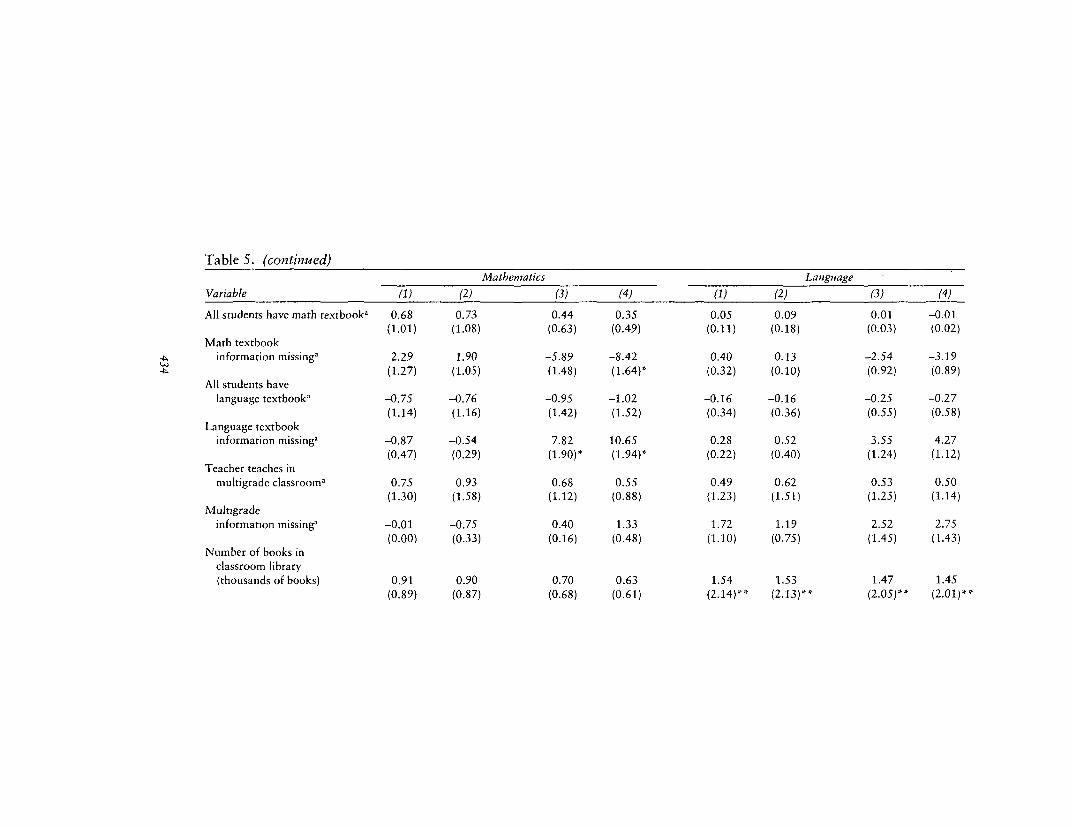
Table 5. (continued)Mathenmatics Langutage
Variable (1) (2) (3) (4) (1) (2) (3) (4)
All students have math textbooka 0.68 0.73 0.44 0.35 0.05 0.09 0.01 -0.01(1.01) (1.08) (0.63) (0.49) (0.11) (0.18) (0.03) (0.02)
Math textbookinformation missinga 2.29 1.90 -5.89 -8.42 0.40 0.13 -2.54 -3.19
(1.27) (1.05) (1.48) (1.64)' (0.32) (0.10) (0.92) (0.89)All students have
language textbooka -0.75 -0.76 -0.95 -1.02 -0.16 -0.16 -0.25 -0.27(1.14) (1.16) (1.42) (1.52) (0.34) (0.36) (0.55) (0.58)
Language textbookinformation missinga -0.87 -0.54 7.82 10.65 0.28 0.52 3.55 4.27
(0.47) (0.29) (1.90)* (1.94)' (0.22) (0.40) (1.24) (1.12)Teacher teaches in
multigrade classroom, 0.75 0.93 0.68 0.55 0.49 0.62 0.53 0.50(1.30) (1.58) (1.12) (0.88) (1.23) (1.51) (1.25) (1.14)
Multogradeinformation missinga -0.01 -0.75 0.40 1.33 1.72 1.19 2.52 2.75
(0.00) (0.33) (0.16) (0.48) (1.10) (0.75) (1.45) (1.43)Number of books in
classroom library(thousands of books) 0.91 0.90 0.70 0.63 1.54 1.53 1.47 1.45
(0.89) (0.87) (0.68) (0.61) (2.14)** (2.13)** (2.05)*$ (2.01)*

Classroom libraryinformation missing, 0.40 0.36 0.40 0.45 0.30 0.27 0.40 0.42
(0.73) (0.67) (0.69) (0.76) (0.79) (0.73) (0.99) (1.01)
Community participation variableNumber of parent association visits
to classroom in past month 0.14 -0.11 0.10 -0.03(1.72)' (0.78) (1.77)* (0.29)
Inverse Mills ratio -0.58 -0.20 -0.05 -0.12 -1.09 -0.82 -0.73 -0.75(0.68) (0.22) (0.06) (0.13) (1.84)* (1.34) (1.20) (1.22)
Constant 3.97 3.45 4.13 4.47 1.12 0.74 0.83 0.92(1.71)* (1.47) (1.75)* (1.87)* (0.69) (0.45) (0.51) (0.55)
Number of observations 605 605 605 605 605 605 605 605Number of municipalities 90 90 90 90 90 90 90 90Overall R2 0.0153 0.0129 0.0173 0.0175 0.0186 0.0010 0.0108 0.0077
* Significant at the 10 percent level.* Significant at the 5 percent level.
* Significant at the 1 percent level.Note: Dependent variable is mathematics or language test score. t-statistics are in parentheses.

436 THE WORLD BANK ECONOMIC REVIEW, VOL. 13, NO. 3
Children with more siblings perform worse on both math and language tests,although the coefficients are not statistically significant. This result may indicatethat parents devote less time to their children's individual needs. Older childrendo better in math than younger ones, even though they are in the same grade.However, age does not matter in determining language scores.
The EDUCO effect can be mediated through school and classroom-level indica-tors and through the intensive involvement of parent associations. To capturethese effects, we include school and classroom-level characteristics and a com-munity participation variable in the regressions."9 The EDUCO effect is less thanthat in regressions without school-level variables, indicating that a significantportion of the difference between EDUCO and traditional schools can be capturedby differences in observable school characteristics and differences in communityinvolvement (see table 4). The EDUCO coefficient, however, is still statisticallyinsignificant. The basic results for the effects of socioeconomic characteristics donot change.
Most of the school-level variables are not significantly different from zero.The two exceptions are teachers' base salary, which has a negative coefficient,and the availability of a classroom library, which is positively related to languageachievement scores. EDUCO teachers receive a piece-wage rate, which the ACES
determine, while teachers in traditional schools have a fixed-wage scheme (WorldBank 1995). The results for teachers' base salary might capture the inefficiencyof fixed wage schemes in traditional schools. The positive effect on languagescores of having a classroom library is also consistent with past evaluation ofEDUCO (World Bank 1995: 19-20). It may be that classroom libraries help teach-ers to complete their lesson plans and stimulate students' interest and readinghabits, both of which improve language scores.
Most notably, the community participation variable has a positive and statis-tically significant coefficient for the basic specification with the EDUCO dummyvariable (see column 2 of table 5). This finding indicates that the intensity ofcommunity involvement is significantly related to students' academic achieve-ments. Community participation might have a positive peer effect or work tomonitor teachers.
IV. EMPIRICAL RESULTS: STUDENT ABSENCE
Parents' negative perceptions of education are an important issue, and this istrue not only in El Salvador. In many rural areas throughout the developing worlduneducated parents underestimate the value of education and thus do not sendtheir children to school. The reasons may be cultural, social, or economic. Themain problem, however, seems to be that parents are given poor incentives or poorinformation. Teacher absenteeism is also a chronic problem in the public schools
19. We enter them linearly and interact them with the EDUCO dummy, since EDUCO may change schoolcharacteristics. We do not report the regressions with the interaction terms here. They are available onrequest.

Jimenez and Sawada 437
of many developing countries. Although excuses are sometimes legitimate, such assickness, more often teachers are simply derelict. When teachers are absent, classesare usually canceled, since there is no tradition of using substitute teachers.
Our hypothesis is that in a decentralized setting parents are better able andmotivated to send children to school and to monitor teacher behavior. In fact,parents are more likely to send their children to school if they attend an EDUCOschool, and teacher absenteeism is less prevalent in EDUCO schools, further reduc-ing student absence (World Bank 1997).
The dependent variable in our regressions is the number of school days that thechild missed in the past month. To control for student absence because of healthproblems, we add an additional indicator variable that equals 1 if a child sufferedfrom a respiratory illness or flu in the past two weeks and 0 otherwise. The princi-pal result is that the coefficients on the EDUCO dummy variable are consistentlynegative and statistically significant, especially if we control for participation bias(table 6). A student in an EDUCO school is less likely to be absent even after we holdconstant household, school, and participation characteristics.20
An important finding is that mother's education has a negative and statisti-cally significant coefficient in all specifications. Having an educated mother re-duces student absence approximately 70 percent. This implies that the mother'spositive perception of education drawn from her own experiences contributes tobetter child attendance.
We also differentiate the EDUCO dummy variables by year. The dummy vari-able for 1991-94 is insignificant-a third-grade student attending an EDUCO schoolduring those years is just as likely to be absent as a student from a traditionalschool (table 6). However, the EDUCO coefficients are negative and significant forschools that were built in 1996 in the regressions with the participation correc-tion. The EDUCO effect is stronger for newer schools, which is consistent with theHawthorne effect described earlier. Thus the negative effect of a decay in earlyenthusiasm of staff and students seems to dominate the positive effect of experi-ence on performance.
The coefficient of the participation correction term is positive, although notsignificant. This means that unobserved characteristics of EDUCO students makethem more likely to miss school.
V. CONCLUSIONS
El Salvador's EDUCO program has been remarkably successful in expandingeducational opportunities for the poor living in rural areas. Decentralization has
20. Teachers are absent more days in traditional schools (1.4 days a month) than in EDUCO schools(1.16 days a month), implying that parent association monitoring works. This finding contrasts with thatof Reimers (1997), who conducted interviews in 140 schools in 1993. That study was done on a earliervintage than the schools in this study and did not correct for other variables that may affect outcomes.Sawada (1998) also extensively investigates the transmission mechanism from community participation tobetter educational outcomes in EDUCO schools by estimating teacher compensation and effort functions, aswell as input demand functions.

438 THE WORLD BANK ECONOMIC REVIEW, VOL. 13, NO 3
Table 6. Municipality Fixed-Effects Regressions of Student AbsenceVariable (1) (2) (3) (4)
EDUCO variablesEDUCO school presenta -3.01 -3.93
(1.79)* (1.91)*EDUCO built in 1991-94a -3.11 -3.55
(1.53) (1.41)EDUCO built in 19953 -2.64 -0.93
(1.32) (0.21)EDUCO built in 1996a -3.20 -4.23
(1.76)* (1.84)*Year missing, -3.89 -5.89
(1.69)* (1.55)Child and household variablesGender (female = 1) -0.08 -0.08 -0.03 -0.03
(0.29) (0.30) (0.10) (0.13)Child's age 0.17 0.17 0.16 0.17
(2.10)** (2.07)** (1.98)** (2.04)**Child lives without parent(s)' -0.12 -0.12 -0.16 -0.21
(0.27) (0.28) (0.36) (0.46)Child had respiratory illness or flu in past
two weeks, -0.29 -0.29 -0.26 -0.26(1.02) (1.02) (0.89) (0.90)
Number of siblings (ages 4-15) -0.11 -0.11 -0.08 -0.08(1.23) (1.23) (0.86) (0.86)
Mother began basic educationa -0.70 -0.68 -0.67 -0.66(2.24)* (2.17)'* (2.13)** (2.09)**
Mother's education missinga -0.23 -0.22 0.13 0.16(0.44) (0.40) (0.23) (0.28)
Father began basic educationa 0.41 0.41 0.36 0.35(1.38) (1.38) (1.21) (1.18)
Father's education missinga -0.58 -0.61 -0.68 -0.75(0.79) (0.81) (0.91) (0.99)
Own housea -0.17 -0.20 -0.24 -0.26(0.53) (0.60) (0.74) (0.79)
Electricity availablea -0.39 -0.39 -0.75 -0.79(1.07) (1.08) (1.93)* (2.02)**
Sanitary service availablea -0.20 -0.22 -0.29 -0.29(0.52) (0.56) (0.71) (0.72)
Water availablea -0.58 -0.57 -0.68 -0.68(0.93) (0.90) (1.06) (1.06)
School variablesTeacher-pupil ratio 27.18 23.95
(0.90) (0.76)Sanitation or latrine available3 -1.87 -1.79
(1.84)-' (1.73)'Electricity availablea 1.38 1.73
(1.95)* (2.06)*'Piped water available- 0.09 0.25
(0.13) (0.37)

Jimenez and Sawada 439
Table 6. (continued)Variable (1) (2) (3) (4)
Teacher and classroom variablesTeacher finished university education3 0.63 1.03
(1.13) (1.48)Years of teacher experience 0.001 0.004
(0.03) (0.08)Monthly base salary of teacher (thousands of colones) 1.08 0.90
(1.88)* (1.47)Teacher receives bonusa -0.17 -0.29
(0.29) (0.48)All students have math textbooka 1.31 1.09
(1.S4) (1.23)Math textbook information missinga 1.50 -3.55
(0.66) (0.55)All students have language textbooka -0.73 -0.82
(0.88) (0.96)Language textbook information missinga -0.23 5.21
(0.10) (0.76)Teacher teaches in multigrade classroom, 0.88 0.60
(1.19) (0.76)Multigrade information missinga -2.93 -0.98
(1.02) (0.28)Number of books in classroom library
(thousands of books) -0.24 -0.30(0.19) (0.23)
Classroom library information missinga -0.50 -0.26(0.74) (0.35)
Community participation variableNumber of parent association visits to classroom 0.07 -0.05
(0.74) (0.26)Inverse Mills ratio 0.96 1.02 1.48 1.59
(0.93) (0.98) (1.34) (1.43)Constant 1.62 1.68 -2.30 -1.89
(1.55) (1.59) (0.78) (0.63)Number of observations 605 605 605 605Number of municipalities 90 90 90 90R2 0.0022 0.0024 0.0067 0.0074
* Significant at the 10 percent level.e* Significant at the 5 percent level.
* Significant at the 1 percent level.Note: Dependent variable is the number of school days student missed in past month. t-statistics are in
parentheses.a. Binary variable equals 1 if response is "yes," 0 otherwise.
also been instrumental in getting families and communities more involved in theirchildren's schooling. But has the program delivered more? This article has evalu-ated EDUCO by determining if it has raised achievement scores and lowered stu-dent absence.
The average scores of EDUCO students on standardized mathematics and lan-guage tests are lower than those of students attending traditional schools. This is

440 THE WORLD BANK ECONOMIC REVIEW, VOL. 3, NO. 3
not surprising since EDUCO students come from disadvantaged backgrounds. Whatis interesting is that, after we control for background and correct for participa-tion bias in the samples, these differences disappear. In fact, the average perfor-mance of EDUCO students on language tests is slightly better than that of tradi-tional school students. The similarity in outcomes holds regardless of how long aschool has participated in the EDUCO program, although newer schools do showan advantage that is not significantly different from zero.
There is considerable variance in performance even after holding constant fortype of school. The most important socioeconomic variables that have a positiveeffect on student achievement are being male, coming from a family with accessto sanitary services, being older, and having fewer siblings. At the school level,the availability of a classroom library has a positive effect on achievement. Mostimportant, coefficients of the parent participation variable are positive and sta-tistically significant in the two specifications that include an EDUCO dummy vari-able. Test results are significantly and positively related to the number of visits byACES or their equivalent.
The number of days students miss is negatively related to intangible EDUCO
effects. In a decentralized setting parents are more motivated to send children toschool and better able to monitor teachers. Parents' education, especially mother'seducation, has a positive impact on student attendance. Moreover, teachers tendto miss fewer days when monitored by parent associations. This, in turn, impliesthat students miss fewer days.
We conclude that the rapid expansion of rural education through EDUCO's
decentralized mechanism has not lowered achievement levels in El Salvador, evenin the most needy parts of the country. In fact, it has improved language scores.The important transmission mechanism is likely to be the community monitor-ing system. Parents' deeper involvement in their children's education may resultin improved attendance and pressure providers to deliver observable inputs. Al-though teachers, parents, and parent associations are not given direct incentivesto raise standardized test scores in mathematics and language, the EDUCO pro-gram has had an overall positive impact. Thus parents' participation in school-based management seems to be an appropriate way of improving education inpoor communities.
REFERENCES
The word "processed" describes informally reproduced works that may not be com-monly available through library systems.
Ainsworth, Martha. 1992. "Economic Aspects of Child Fostering in C6te d'Ivoire." Liv-ing Standard Measurement Study Working Paper 92. World Bank, Washington, D.C.Processed.
Cox, Donald, and Emmanuel Jimenez. 1991. "The Relative Effectiveness of Private andPublic Schools: Evidence from Two Developing Countries." Journal of DevelopmentEconomics 34(1):99-121.

Jimenez and Sawada 441
El Salvador, MINED (Ministerio de Educaci6n). 1995. EDUCO Learns and Teaches. SanSalvador: Algier's Impresores.
.1997. "Informe de evaluaci6n del rendimiento en 3O, 4o, 6o grado de educaci6nbisica en lenguaje, matemitica, estudios sociales, y ciencia, salud, y medio ambientebasado en la aplicaci6n nacional de pruebas de octubre de 1996." Direcci6n Nacionalde Evaluaci6n e Investigaci6n, San Salvador, February. Processed.
Glewwe, Paul, and Hanan Jacoby. 1994. "Student Achievement and Schooling Choice inLow-Income Countries: Evidence from Ghana." Journal of Human Resources29(3):841-64.
Greene, William H. 1997. Econometric Analysis. 3d ed. Upper Saddle River, New Jersey:Prentice Hall.
Hanushek, Eric A. 1995. "Interpreting Recent Research on Schooling in Developing Coun-tries." The World Bank Research Observer 10(2):227-46.
James, Estelle, Elizabeth King, and Ace Suryadi. 1996. "Finance, Management, andCosts of Public and Private Schools in Indonesia." Economics of Education Review15(4):387-98.
Jimenez, Emmanuel, and Vicente Paqueo. 1996. "Do Local Contributions Affect the Ef-ficiency of Public Primary Schools?" Economics of Education Review I5(4):377-86.
Levin, Henry M. 1997. "Raising School Productivity: An X-efficiency Approach." Eco-nomics of Education Review 16(3):303-11.
Lockheed, Marlaine, and Adriaan Verspoor. 1991. Improving Education in DevelopingCountries. New York: Oxford University Press for the World Bank.
Maddala, G. S. 1983. Limited-Dependent and Qualitative Variables in Econometrics.Cambridge, U.K.: Cambridge University Press.
McMillan, Robert. 1999. "Parental Pressure and Competition: An Empirical Analysis ofPublic School Quality." Department of Economics, Stanford University, Stanford, Calif.Processed.
Reimers, Fernando. 1997. "The Role of the Community in Expanding Educational Op-portunities: The EDUCO Schools in El Salvador." In James Lynch, Celia Modgil, andSohan Modgil, eds., Education and Development: Tradition and Innovation, Equityand Excellence. vol. 2. London: Cassell.
Sawada, Yasuyuki. 1998. "Community Participation, Teacher Effort, and EducationalOutcomes: A Case Study of El Salvador's EDUCO Program." Department of Econom-ics, Stanford University, Stanford, Calif. Processed.
Willis, Robert, and Sherwin Rosen. 1979. "Education and Self-Selection." Journal ofPolitical Economy 87(5):57-36.
World Bank. 1994. "El Salvador: Community Education Strategy: Decentralized SchoolManagement." Country Report 13502-ES. Washington, D.C. Processed.
- . 1995. "Staff Appraisal Report: El Salvador Basic Education ModernizationProject." IBRD Report 14129-ES. Washington, D.C. Processed.
.1996. "Impact Evaluation of Education Projects Involving Decentralization andPrivatization." Working Paper on Impact Evaluation of Education Reforms 0. El Sal-vador Evaluation Team, Washington, D.C. Processed.
.1997. "El Salvador's EDUCO Program: A First Report on Parents' Participation inSchool-based Management." Working Paper on Impact Evaluation of Education Re-forms 4. El Salvador Evaluation Team, Washington, D.C. Processed.


THE WORLD BANK ECONOMIC REVIEW, VOL. 13, NO. 3: 443-65
Can Private School Subsidies Increase Enrollment forthe Poor? The Quetta Urban Fellowship Program
Jooseop Kim, Harold Alderman, and Peter F. Orazem
This study evaluates a program designed to stimulate girls' schooling through the cre-ation of private girls' schools in poor urban neighborhoods of Quetta, Pakistan. Enroll-mentgrowth in these randomly selected neighborhoods is cempared to enrollment growthin otherwise similar neighborhoods that were randomly assigned to a control group.The analysis indicates that the program increased girls' enrollment around 33 percent-age points. Boys' enrollment rose as well, partly because boys were allowed to attendthe new schools and partly because parents would not send their girls to school withoutalso educating their boys. This outcome suggests that programs targeted at girls can alsoinduce parents to invest more in their boys. The success of the program varied acrossneighborhoods, although success was not clearly related to the relative wealth of a neigh-borhood or to parents' level of education. Thus the program offers tremendous promisefor increasing enrollment rates in other poor urban areas.
Private schooling, often postulated to improve school quality, may also be a meansto leverage public funds in order to provide access to schooling at rates fasterthan are possible with public funds alone. This article measures the impact onenrollment of a program designed to encourage the creation of new private girls'schools in Quetta, the capital city of Balochistan Province in Pakistan. The analy-sis represents a unique opportunity to apply experimental design methods toevaluate an educational policy innovation. By randomizing the implementationof the pilot program, we are able to generate robust estimates of the impact of theprogram on enrollment. We avoid the bias that often arises in such assessments
Jooseop Kim is senior researcher at the Korea Institute for Vocational Education and Training, Peter F.Orazem is with the Department of Economics at Iowa State University, and Harold Alderman is with theDevelopment Research Group at the World Bank. Their e-mail addresses are [email protected],[email protected], and [email protected]. This study was supported by the research project ImpactEvaluation of Education Projects Involving Decentralization and Privatization under RPO 679-18 of theWorld Bank, supervised by Elizabeth King. The authors are indebted to current and past members of theBalochistan Primary Education Directorate, including Ijaz Ahmed Malik, Mohammed Ishaque, QuaratulAm, and Bill Darnell, for their kind hospitality and research support. They are also grateful to SultanMahmood Niazi of the Balochistan Education Foundation and to Brian Spicer and Fahim Akbar of theBalochistan Management Information System for their help in designing and implementing the datacollection. Finally, the authors thank their task managers from the South Asia Division, Mae Chu Chang,Guilherme Sedlacek, and Ivar Andersen, for offering many helpful comments and providing an unusuallysupportive research environment amid ongoing operational support; the referees for making valuablesuggestions; and Donna Otto for preparing the final manuscript.
(© 1999 The International Bank for Reconstruction and Development/ THE WORLD BANK
443

444 THE WORLD BANK ECONOMIC REVIEW, VOL 13, NO. 3
when individuals or groups who participate in a program are those who are bestsuited to benefit from it.
I. THE QUETTA GIRLS FELLOWSHIP PROGRAM
Primary school enrollment rates in Pakistan are lower than in other countriesat the same level of economic development, including Bangladesh, India, andNepal. Nationally, the gross enrollment rate is 58 percent: 69 percent for boysand 42 percent for girls. This gender gap is even wider in the province ofBalochistan, where 62 percent of boys and only 29 percent of girls are enrolled inschool.' The government of Pakistan has set a target of achieving universal pri-mary enrollment by 2006. Meeting this goal would require girls' enrollment tomore than double nationally and more than triple in Balochistan.
There is evidence that supply constraints partially account for low school en-rollment and achievement in Pakistan, especially in rural areas and in poor urbanneighborhoods.2 However, in Pakistan, as in many other countries, the govern-ment's ability to increase school capacity is constrained by inadequate publicbudgets. Expansion is also circumscribed because the government generally con-structs, rather than rents, school capacity and requires recipient neighborhoodsto provide land for their new government schools. Many poor urban neighbor-hoods have developed as squatter communities that have poorly defined prop-erty rights, limiting their ability to donate land.
In the case of educating girls, the problem is not the lack of schools per se.Cultural prohibitions in many communities mean that educational opportuni-ties for girls are frequently restricted in the absence of gender-specific programs.If Pakistan is to achieve universal primary enrollment for girls, more segregatedgirls schools or coeducational schools with female teachers will be needed. Giventhe limitations on increased government provision, one strategy is to make pri-vate girls schools more available in poor neighborhoods. Private schools do notface the same problem of land acquisition and may be less constrained finan-cially than government schools. Consequently, the government may devote lesstime and expense to increasing school capacity for girls if it partially funds theexpansion of private schools rather than fully funds the expansion of govern-ment schools.
Recognizing these concerns, the Balochistan Education Foundation launchedthe Urban Fellowship Program in Quetta in February 1995. The purpose ofthis pilot project was to determine whether establishing private schools in poorneighborhoods was a cost-effective means of expanding primary education for
1. These statistics are based on 1996 data provided by the Pakistan Education Management InformationSystem.
2. Alderman and others (1996) find that differences in school availability account for 30-40 percent ofthe gap in cognitive skills between boys and girls in rural Pakistan.

Kim, Alderman, and Oraze7n 445
girls in Quetta's lower-income neighborhoods. Recent evidence from the Paki-stan Integrated Household Survey suggests that about 77 percent of girls whostart school finish the primary cycle. It was thought that if the program couldget these poor girls to start school, many would persist long enough to attainliteracy.
The Urban Fellowship Program encouraged private schools, which were con-trolled by the community, to establish new facilities by paying subsidies directlyto the schools. Schools were assured of government support for three years. Theinitial subsidy was 100 rupees (about $3) per month per girl enrolled. There wasan upper scholarship limit of 10,000 rupees (100 girls at 100 rupees per girl) permonth. This subsidy was sufficient to cover typical tuition at the lowest-pricedprivate schools. In addition, each school received 200 rupees per girl to defraystart-up costs. The subsidy was reduced in the second year and again in the thirdyear. By the fourth year schools were expected to be largely self-sufficient throughfees and private support, although they would still be eligible to apply to theBalochistan Education Foundation for additional grants. It is possible that un-certainty regarding the schools' long-term sustainability discouraged some par-ents from enrolling their children. Nevertheless, even if the results presented hereare a lower bound, they are substantial. We discuss the issue of sustainability inthe concluding section.
Fellowship schools were allowed to admit boys provided that they made upless than half of total enrollment. Boys had to pay tuition at least equal to, andoften greater than, that of girls. The grant was calculated only for enrolled girls;schools received no additional subsidy for enrolling boys. Schools were requiredto keep class sizes at or below 50 boys and girls per classroom and had to hire atleast one teacher for each classroom.
To implement the program, the Balochistan Education Foundation contractedthe Society for Community Support of Primary Education in Balochistan (SCSPEB),
a nongovernmental organization (NGO), to conduct an initial census of each siteto ensure that there were a sufficient number of girls in the target age range (fourto eight years) and to inform parents of the program. The SCSPEB had severalyears of experience in implementing primary school projects, particularly schoolpromotion efforts in rural communities. The goal was to create a partnershipbetween neighborhood parents and the school operator. The SCSPEB first con-ducted a meeting of parents to see if they were interested in attracting a privateschool to their neighborhood. The parents were asked to form a committee, whichwould represent the neighborhood in negotiations with potential school opera-tors. With the assistance of the SCSPEB, the parent committee developed a pro-posal detailing the neighborhood's need for a school, the resources it was willingto provide the school (land, buildings, equipment), and any other requirementsan operator was expected to satisfy. Experienced school operators were invitedto submit proposals in response. The parent committees were allowed to selecttheir school operator from among the proposals or to choose to run the schoolthemselves.
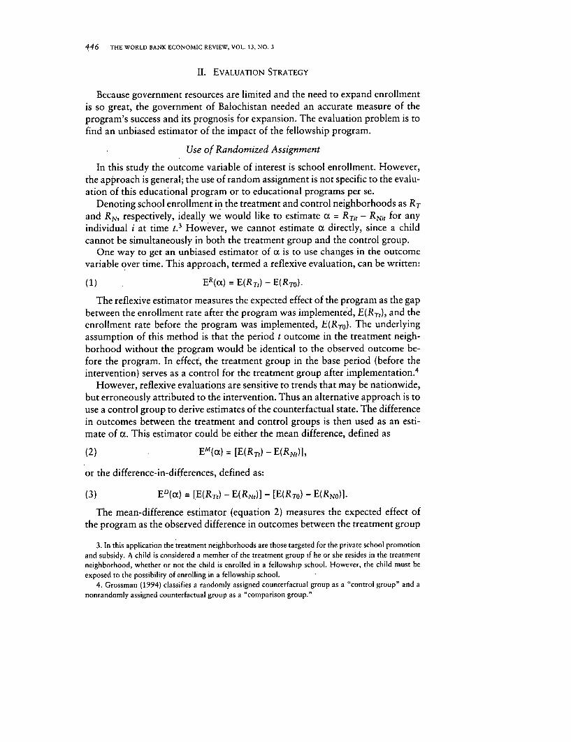
446 THE WORLD BANK ECONOMIC REVIEW, VOL. 13, NO. 3
II. EVALUATION STRATEGY
Because government resources are limited and the need to expand enrollmentis so great, the government of Balochistan needed an accurate measure of theprogram's success and its prognosis for expansion. The evaluation problem is tofind an unbiased estimator of the impact of the fellowship program.
Use of Randomized Assignment
In this study the outcome variable of interest is school enrollment. However,the approach is general; the use of random assignment is not specific to the evalu-ation of this educational program or to educational programs per se.
Denoting school enrollment in the treatment and control neighborhoods as RT
and RN, respectively, ideally we would like to estimate a = RTi, - RN,t for anyindividual i at time t.3 However, we cannot estimate a directly, since a childcannot be simultaneously in both the treatment group and the control group.
One way to get an unbiased estimator of a is to use changes in the outcomevariable over time. This approach, termed a reflexive evaluation, can be written:
(1) , ER(Ct) = E(RTt) - E(Rmo).
The reflexive estimator measures the expected effect of the program as the gapbetween the enrollment rate after the program was implemented, E(RT,), and theenrollment rate before the program was implemented, E(RTO). The underlyingassumption of this method is that the period t outcome in the treatment neigh-borhood without the program would be identical to the observed outcome be-fore the program. In effect, the treatment group in the base period (before theintervention) serves as a control for the treatment group after implementation.4
However, reflexive evaluations are sensitive to trends that may be nationwide,but erroneously attributed to the intervention. Thus an alternative approach is touse a control group to derive estimates of the counterfactual state. The differencein outcomes between the treatment and control groups is then used as an esti-mate of a. This estimator could be either the mean difference, defined as
(2) EM(a) = [E(RTt) - E(RNd)]
or the difference-in-differences, defined as:
(3) ED(a) = [E(RTt) - E(RNt)] - [E(RTO) - E(RNO)1-
The mean-difference estimator (equation 2) measures the expected effect ofthe program as the observed difference in outcomes between the treatment group
3. In this application the treatment neighborhoods are those targeted for the private school promotionand subsidy. A child is.considered a member of the treatment group if he or she resides in the treatmentneighborhood, whether or not the child is enrolled in a fellowship school. However, the child must beexposed to the possibility of enrolling in a fellowship school.
4. Grossman (1994) classifies a randomly assigned counterfactual group as a "control group" and anonrandomly assigned counterfactual group as a 'comparison group."
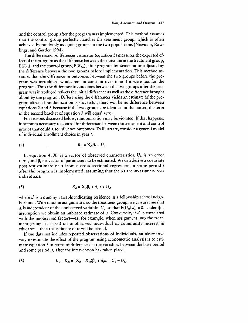
Kim, Alderman, and Orazem 447
and the control group after the program was implemented. This method assumesthat the control group perfectly matches the treatment group, which is oftenachieved by randomly assigning groups to the two populations (Newman, Raw-lings, and Gertler 1994).
The difference-in-differences estimator (equation 3) measures the expected ef-fect of the program as the difference between the outcome in the treatment group,E(RT,), and the control group, E(RNt), after program implementation adjusted bythe difference between the two groups before implementation. This method as-sumes that the difference in outcomes between the two groups before the pro-gram was introduced would remain constant over time if it were not for theprogram. Thus the difference in outcomes between the two groups after the pro-gram was introduced reflects the initial difference as well as the difference broughtabout by the program. Differencing the differences yields an estimate of the pro-gram effect. If randomization is successful, there will be no difference betweenequations 2 and 3 because if the two groups are identical at the outset, the termin the second bracket of equation 3 will equal zero.
For reasons discussed below, randomization may be violated. If that happens,it becomes necessary to control for differences between the treatment and controlgroups that could also influence outcomes. To illustrate, consider a general modelof individual enrollment choice in year t:
(4) Ri,,,: t + U,,
In equation 4, Xi, is a vector of observed characteristics, Uit is an errorterm, and p,is a vector of parameters to be estimated. We can derive a covariatepost-test estimate of a from a cross-sectional regression in some period tafter the program is implemented, assuming that the as are invariant acrossindividuals:
(5) R,= Xitt + d,a+ U+t
where d, is a dummy variable indicating residence in a fellowship school neigh-borhood. With random assignment into the treatment group, we can assume thatd, is independent of the unobserved variables U,,, so that E( U,t I d,) = 0. Under thisassumption we obtain an unbiased estimate of cc. Conversely, if d, is correlatedwith the unobserved factors-as, for example, when assignment into the treat-ment groups is based on unobserved individual or community interest in'educaton-then the estimate of a will be biased.
If the data set includes repeated observations of individuals, an alternativeway to estimate the effect of the program using econometric analysis is to esti-mate equation 5 in terms of differences in the variables between the base periodand some period, t, after the intervention has taken place.
(6) R,t- R,o = (X,, - XiO)PO + d,a + U,, - U1o.
448 THE WORLD BANK ECONOMIC REVIEW, VOL. 13, NO. 3
Gender Differences in Enrollment Response
Parents may make different schooling investments in girls and boys either be-cause costs differ or because parents obtain different benefits from educatinggirls and boys. Differences in costs may not just be differences in fees. Gender-specific costs may reflect differences in school access, the opportunity cost of aboy's or girl's time, or any disutility parents suffer because of cultural pressuresagainst sending their daughters to school.
International experience indicates that returns in terms of proportional in-creases to household and wage productivity generally do not differ appreciablyby gender even when average wages or patterns of labor participation do (Behrmanand Deolalikar 1995; Schultz 1995). However, differences in how parents assessreturns to schooling may also reflect how they benefit from the human capital oftheir daughters. Their assessment may reflect marriage and residency patterns aswell as gender differences in remittances across generations. Nevertheless, Alder-man and King (1998) indicate that for many purposes, including that of the presentstudy, reduced-form models of investment in schooling are identical, regardlessof whether the gender difference in education reflects differences in costs or dif-ferences in how parents value the gains from schooling boys and girls.
The girls fellowship program raises the cost of schooling in terms of fees (ru-pees) but lowers it in terms of travel time. In addition, it may also lower thecultural disutility of educating girls, which has the same impact as lowering therupee price. Since all of the preexisting schooling options are still available to thefamily, the net impact of adding the new choice should be an increase in school-ing for girls.5
The impact of the fellowship program on boys' enrollment is, however, am-biguous. Lowering the price of girls' schooling may lead to a substitution of girls'time for boys' time, with girls spending more time outside the home and boysdevoting more time to home production. But there are at least two reasons whythe fellowship program may have a positive impact on boys' schooling. First, theprogram creates a new low-priced private school that can accept boys. Second,boys' education may -increase as their sisters go to school for a very practicalreason: parents may want their sons to escort their sisters to and from school.Thus boys' and girls' education may be complementary goods.
If factors that affect enrollment, such as income, the cost of schooling, and thedisutility of sending girls to school, differ systematically across treatment andcontrol neighborhoods, they may affect the apparent impact of the program.Thus the econometric specification of equations 5 and 6 includes three measuresof schooling costs: the fees charged in the preexisting neighborhood schools; av-
5. Becker (1981: ch. 6) develops a model of human capital investment in children that highlightsparents' incentives to equalize wealth among their children. His model suggests that neutral parents investmore in less fortunate children so that all of their children are equally well off. Of course, there is considerableevidence that parents favor boys over girls. Kim, Alderman, and Orazem (1998) analyze the impact ofreducing the price of girls' schooling on boys' and girls' enrollment when parents favor hoys over girls atequal schooling prices.

Kim, Alderman, and Orazem 449
erage distance to schools, measured in minutes of travel time (a proxy for trans-port costs); and the child's age, which may determine the opportunity cost of thechild's time. The specification also includes the father's and mother's education,which are assumed to influence how a household values returns to schooling. Inaddition, the preference for education may depend on the child's birth order(parents may have a preference for educating the eldest child, particularly theeldest boy) and on citizenship (refugees may have different expectations of re-turns to education).6 These variables, along with household income and the child'sgender, make up the vector of exogenous variables we use in our analysis.
III. DATA
Only a modest number of treatment groups was available because only 10pilot sites were initially funded. For political expediency the government opted toplace one neighborhood school in each of 10 urban slum areas of Quetta, ensur-ing that all major ethnic groups received at least one school. To accommodatethis plan, the sample includes a degree of stratification, under which randomiza-tion is based on neighborhoods within each slum area.
A second problem is that no recent census of the population had been con-ducted from which to define treatment and control populations. The most recentcensus was 14 years old. The population of Quetta is estimated to have grown atabout 7 percent a year since then, mainly within the neighborhoods that made upthe target population. Consequently, the designers of the program chose an areaframe sampling strategy to define the treatment and control neighborhoods.
They designed the area frame as follows. On a map of Quetta they outlinedeach of the 10 slum areas, selecting three sites in each, literally points on the map.They then randomly chose one of these areas to be the treatment neighborhoodfor the creation of a private school. Because all neighborhoods selected to partici-pate accepted the invitation, the issue of self-selection was moot. The other neigh-borhoods became controls. The only criterion for the treatment neighborhoodwas that it could not already have a government girls' school. Although the con-trol sites could have had a government girls' school, none of them did.
Given the small number of pilot sites, it is useful to see if the treatment andcontrol populations differ in the factors that might also cause enrollment out-comes to differ. Such tests also help to determine which household characteristicscontribute to program participation.
The baseline data collected in the treatment and control sites include informa-tion on households' socioeconomic characteristics, parents' education, and theeducational attainment and current enrollment status of all children in the house-hold. All of the households in treatment neighborhoods were surveyed in thesummer of 1994, when the scholarship program was being promoted and before
6. Intrahousehold allocation of schooling is discussed in Parish and Willis (1993) and Butcher andCase (1994).

450 THE WORLD BANK ECONOMIC REVIEW, VOL. 13, NO. 3
any fellowship schools were opened. The baseline survey of households in thecontrol neighborhoods was conducted in July 1995. Because most of the data onhousehold socioeconomic status do not change over a short period-no majoreconomic transformation occurred in 1994 or 1995-the difference in the timingof the surveys should not be problematic. Information on the enrollment statusof children in control neighborhoods was obtained for 1995 and retrospectivelyfor the previous year.' Enrollment data were subsequently collected in 1996 inboth treatment and control neighborhoods. The Balochistan Education Manage-ment Information System supervised all data collection and training of surveyorsto ensure comparability of the data.
In this article we measure the program's impact using the estimators describedin equations 1-6. By doing so, we can ascertain whether the results are robust.Moreover, we apply each of these estimators in two ways. First, we measure thechange in enrollment for children in the target range of five to eight years. Sec-ond, we measure enrollment rates longitudinally for children ages four to sevenin the initial year of the fellowship program.
IV. RESULTS
The treatment sample includes 1,310 children, 781 girls and 529 boys (table1). The control sample includes 1,358 children, 697 girls and 661 boys. Thedependent variable in table 1 is a dummy variable that equals 1 if the child wasenrolled in school. The other variables are exogenous variables believed to affectparents' enrollment choices for their children. Most of the variables come di-rectly from the questionnaire. However, distance to school and annual fees areneighborhood averages 'of the children in school. We estimate household incomeusing the number of adults in the household, their educational attainment, and aset of household assets. Details on the estimate of household income are con-tained in the appendix.
We test for statistical significance of the differences between the treatment andthe control groups in two ways.8 First, in order to determine if the randomizationyielded observationally equivalent treatment and control populations, we test forthe equality of means of the endogenous and exogenous variables. Second, weestimate enrollment equations using the baseline data. These equations test thenull hypothesis of the equality of behavioral coefficients in the enrollment choicemodels for the treatment and control neighborhoods.
7. Collecting data retrospectively raises the possibility of recall bias, although parents should be able toremember whether their children were in school a year earlier. To verify this, we use multiple methods toevaluate the change in enrollment in the treatment neighborhoods. We find that the conclusions are notsensitive to differences in evaluation method.
8. Newman, Rawlings, and Gertler (1994) point out that researchers rarely test for statistical significanceof the differences, so that probabilities of receiving a program may not be equal for individuals orcommunities in many of the evaluation studies in developing countries, especially those with few observationsin the treatment group.

Kim, Alderman, and Orazem 451
Table 1. Summary Statistics of Baseline Data and Tests of the Equality ofMeans between Treatment and Control Groups
Girls Boys
Variable Treatment Control t-value' Treatment Control t-value'
EndogenousEnrollment rate 0.366 0.300 2.67 0.486 0.398 3.03
(0.482) (0.459) [1,468] (0.500) (0.490) [1,180]
ExogenousHousehold income 7,108 6,808 1.03 7,005 6,592 1.41
(7,157) (3,011) [1,476] (6,815) (2,847) [1,188]Age 6.026 6.001 0.19 6.040 6.003 0.44
(1.403) (1.429) [1,476] (1.426) (1.444) [1,188]Mother's highest grade 0.619 0.395 2.08 0.623 0.414 1.74
(2.243) (1.844) [1,466] (2.208) (1.918) [1,183]Father's highest grade 3.405 3.079 1.27 3.635 2.723 3.38
(4.745) (4.882) [1,417] (4.579) (4.548) [1,162]Birth order 2.832 3.004 2.21 3.074 2.965 1.27
(1.474) (1.510) [1,476] (1.447) (1.482) [1,188]Citizenship 0.868 0.835 1.79 0.877 0.814 2.98
(0.339) (0.371) [1,476] (0.329) (0.389) [1,188]Distance to school 17.77 17.81 0.05 16.93 16.42 0.62
(9.443) (9.991) [491] (9.338) (9.394) [515]Annual fees 244.3 187.0 1.19 531.3 391.7 1.73
(536.0) (502.5) [480] (1,036.8) (765.1) [505]Joint testb 9.0 27.2Number of observations 781 697 529 661
Note: Sample includes girls and boys ages four to eight in the baseline year. The baseline data werecollected in 1994 for the treatment group and in 1995 for the control group. The numbers in parenthesesare the standard deviations corrected for cluster effects using Huber's method. The numbers in squarebrackets are the degrees of freedom. The degrees of freedom differ because of missing information in thesurveys.
a. The null hypothesis is that the mean of the variable in the treatment group is equal to that in thecontrol group. if the z-value is smaller than 1.96, the null hypothesis caniot be rejected at the 5 percentsignificance level.
b. Corrected F-statistics with degrees of freedom (8, 1,376) for girls and (8, 1,149) for boys. The nullhypothesis is that the means of the eight exogenous variables are jointly equal across the treatment andcontrol neighborhoods. For both boys and girls the test statistic exceeds the critical value of 1.94 at the 5percent significance level.
Source: Authors' calculations.
Baseline enrollment rates for both sexes are significantly higher in the treat-ment group than in the control group (columns 4 and 7 of table 1).9 In addition,birth order and mother's education differ significantly between girls in the treat-ment and control neighborhoods, although the differences in means are smallnumerically. For boys, citizenship and father's education are significantly higher
9. It is unclear why girls' enrollment rates are 6 percentage points higher in the treatment neighborhoods,although we do not believe that the 10 fellowship school sites were strategically selected. Of the girls inschool, 39 percent attended private school and 61 percent attended government boys' schools. The largeproportion in private school is not unusual, especially given the limited availability of government schools.Alderman, Orazem, and Paterno (1996) also find that poor households in Lahore, Pakistan, used privateschools extensively.

Table 2. Baseline Probit Analysis of the Probability of EnrollmentGirls and boys Girls Boys
Variable Treatment Control Difference, Treatment Control Differencea Treatment Control Difference'
Household income per10,000 rupees 0.138 0.422 2.03 0.171 0.572 2.58 0.037 0.218 0.25
(2.362) - (2.879) (2.377) (2.870) (0.346) (0.954)Age 1.820 2.235 0.09 1.611 2.623 0.02 2.176 1.927 0.14
(5.226) (6.323) (3.612) (4.864) (3.674) (3.986)Age squared -0.101 -0.140 0.89 -0.089 -0.174 0.47 -0.119 -0.119 0.99
(3.621) (5.014) (2.508) (4.127) (2.513) (2.884)Mother's highest grade 0.051 0.094 1.50 0.067 0.118 0.73 0.007 0.072 1.95
(2.443) (3.422) (2.500) (2.649) (0.197) (1.963)Father's highest grade 0.023 0.065 7.68 0.027 0.084 6.88 0.025 0.050 1.09
(2.369) (6.634) (2.271) (5.997) (1.498) (3.500)Birth order -0.029 -0.036 0.07 -0.017 -0.020 0.00 -0.036 -0.053 0.04
(0.918) (1.214) (0.416) (0.461) (0.717) (1.251)Citizenship 0.693 0.335 1.20 0.628 0.214 1.36 0.762 0.538 0.00
(5.207) (2.556) (3.590) (1.079) (3.545) (2.888)Girl -0.419 -0.541 0.05
(4.878) (5.340)Number of observations 1,231 1,324 725 677 506 647Joint testb 29.9 23.3 13.7Pseudo R2 0.277 0.295 0.230 0.331 0.358 0.293
Note: The numbers shown in parentheses are z-values corrected for cluster effects using Huber's method.a. Test of the difference in coefficients between treatment and control neighborhoods, corrected for cluster effects using Huber's method.b. Joint chi-square test of the null hypothesis of equality of coefficients across treatment and control neighborhoods. All results reject the null hypothesis of equality.Source: Authors' calculations.
Kim, Alderman, and Orazem 453
in the treatment group, although, again, the differences in means are small nu-merically. The joint test that the means of the exogenous variables are equalacross all variables is easily rejected for both boys and girls. Therefore, we canreach a statistical conclusion that the treatment and control samples are not iden-tical, a problem that we address in the analysis below.
A second way in which the treatment and control neighborhoods may differ isin parents' decisionmaking processes. To check this, we estimate a probit model ofschool enrollment based on equations 8-9 (table 2). The estimated parameters forthe control and treatment groups exhibit the same signs and are qualitatively simi-lar to results obtained in other studies of enrollment. The coefficient on householdincome is positive in both samples. Mother's and father's educational attainmentpositively influence their children's enrollment. Enrollment increases with age, butat a diminishing rate. First-born children have a higher probability of enrollingthan their younger siblings, but the coefficient is not significant. Native Pakistanisalso have a higher probability of enrolling than noncitizens. After pooling the treat-ment and control data, we can also estimate the effects of the average distance toschool and average annual fees. Both have negative coefficients, except for a posi-tive but insignificant effect of annual fees on boys' schooling.
The coefficients for the two groups are not statistically different, except forfather's educational level in the girls' enrollment equation.1 ' This result suggeststhat parents' decisions about education are similar in the treatment and controlneighborhoods. Despite significant differences in characteristics between the con-trol and treatment groups (as reported in table 1), we can still measure the changein enrollment due to the program by measuring the difference in enrollment ratesbetween treatment and control groups, holding constant the differences in theexogenous variables.
Comparisons of Mean Enrollment Rates
Using enrollment rates for boys and girls before and after the program inter-vention (table 3), we can apply the three methods based on equations 1-3 (table4). We report both age-specific and cohort-specific effects. The age-specific analysislooks at the enrollment of children ages five to eight in a specific year, while thecohort-specific analysis follows the enrollment of a fixed group of children agesfour to seven in 1994.11
The age-specific results are similar for the three methods. All imply that thefellowship program had a positive effect on the enrollment of girls in the targetage group as well as on that of boys. Applying the same methods to two years ofdata yields even larger estimates of the enrollment effects.
10. See Kim, Alderman, and Orazem (1998) for details of the statistical tests.11. The cohort-specific enrollment rates in 1994 are lower than the 1994 average for the age-specific
enrollment rates. The reason is that the age-specific groups are on average one year older in 1994. By 1996the enrollment rates in the cohort-specific groups are higher than in the age-specific groups because, bythen, the cohort-specific groups are on average one year older than the age-specific groups.
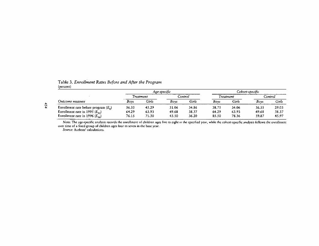
Table 3. Enrollment Rates Before and After the Program(percent)
Age-specific Cohort-specificTreatment Control Treatment Control
Outcome measure Boys Girls Boys Girls Boys Girls Boys Girls
Enrollment rate before program (E0) 56.33 45.29 51.06 34.86 38.75 34.06 36.55 29.03Enrollment rate in 1995 (Eg5) 64.29 63.93 49.68 38.37 64.29 63.93 49.68 38.37Enrollment rate in 1996 (E96) 76.15 71.30 43.50 36.20 85.50 78.36 59.87 45.97
Note: The age-specific analysis records the enrollment of children ages five to eight in the specified year, while the cohort-specific analysis follows the enrollmentover time of a fixed group of children ages four to seven in the base year.
Source: Authors' calculations.

Table 4. Age- and Cohort-Specific Effects of the Fellowship Program on Enrollment RatesAge-specific Cohort-specific
Estimation method Mathematical expression Boys Girls Boys Girls
Measure of effect using meansReflexive (1994-95) ER (a) = E(RT,) - E(Ro). 8.0 18.6 25.5 29.9
(0.42) (0.44) (0.43) (0.44)Reflexive (1994-96) ER (a) = E(RT,) - E(R,). 19.8 26.0 46.8 44.3
(0.51) (0.53) (0.52) (0.54)Difference-in-differences (1994-95) ED (a) = [E(RT,) - E(RN,)I - [E(Rr) - E(RNO)]. 9.3 15.1 12.4 20.5
(0.53) (0.54) (0.54) (0.54)Difference-in-differences (1994-96) ED (a) = [E(RT,) - E(RN,)] - [E(RT,) - E(RNO)]. 27.4 24.8 23.4 27.4
(0.73) (0.70) (0.74) (0.71)Mean-difference (1994-95) EM (a) = [E(Rr,) - E(RNt)]. 14.6 25.6 14.6 25.6
(0.65) (0.67) (0.65) (0.67)Mean-difference (1994-96) EM (a) = [E(RT,) - E(RN,)]. 32.7 35.1 25.6 32.4
(0.59) (0.65) (0.60) (0.66)
Measure of effect using regressionCovariate post-test (1995 cross-sectional) R,, = X,, P, + d,a, + U., 22.4 33.4 22.4 33.4
(0.04) (0.03) (0.04) (0.03)Covariate post-test (1996 cross-sectional) R,, = Xj, , + d,a, + U,, 38.4 42.7 26.8 39.9
(0.07) (0.05) (0.05) (0.04)First-difference, time-invariant j (1994-95) R,, - Ro = d,cx, + U,, - U,O 29.2 36.7
(0.08) (0.07)First-difference, time-invariant 1 (1994-96) R,,- Rro= da,+ U,, - U,O 8.8 26.4
(0.10) (0.08)First-difference, time-varying 1 (1994-95) R,,- R,0 = X,(P,- P,.>) + d,a,+ U,,0- U, 42.8 46.9
(0.11) (0.08)First-difference, time-varying 1 (1994-96) R,,- R,O= X,(0,- -2) + d,a,+ U,,- U,O 24.2 28.1
(0.14) (0.10)
Note: Numbers in parentheses are standard errors corrected for cluster effects using Huber's method.Source: Authors' calculations.

456 THE WORLD BANK ECONOMIC REVIEW, VOL. 13, NO. 3
The cohort-specific analysis has the advantage of enabling us to control forunobservable effects that are specific to the individual and that might also becorrelated with program outcomes. However, because enrollment increases withage, at least initially, some of the enrollment growth in the cohort-specific analy-sis will reflect a maturity effect. This effect will bias the reflexive method esti-mates upward. Indeed, the implied 46.8 percent increase in boys' enrollment,and 44.3 percent increase in girls' enrollment between 1994 and 1996 (the lasttwo columns of table 4) are much higher than the corresponding estimates in theage-specific analysis.
The estimates generated from the difference-in-differences and mean-difference methods eliminate the maturity effect by assuming that it is commonacross neighborhoods. Consequently, the measured program effects using thesemethods are smaller than the reflexive estimates and are more comparable to theestimates generated with the age-specific sample. All of the results show largegains in both boys' and girls' enrollment following the opening of the fellowshipschools. Most estimates show slightly higher enrollment gains for girls than forboys. Looking across the age-specific and cohort-specific estimates, we can con-clude that girls' enrollment rose 25-35 percent as a result of the program andthat boys' enrollment rose a few percentage points less.
Comparisons Using Regression Analysis
Because the treatment and control neighborhoods have different characteris-tics that are believed to affect parents' educational choices, a simple comparisonof unconditional means could yield biased estimates of the program effect. Weuse an alternative method based on equation 5 on the same samples.' 2 The pro-gram effects based on the covariate post-test using cross-sectional data are re-ported in table 4; the full probit regression results are in table 5. The enrollmentrate in fellowship neighborhoods rose 33.4 percent for girls and 22.4 percent forboys in the first year of the program (table 4). After two years enrollment in thefellowship neighborhoods had risen 42.7 percent for girls and 38.4 percent forboys using the age-specific analysis. The gain was slightly less using the cohortanalysis. These results are consistent with the results based on community means.
Considering that the fellowship schools were established in February 1995and that survey data were collected in July of that year, the response of parents intarget areas was nearly instantaneous. This supports the view that there wasexcess demand for primary education in these poor areas. Moreover, the fellow-ship program grew more successful year by year. For girls the estimated programeffect increased almost 10 percent in 1996 relative to the effect in 1995. Boys'enrollment rates grew 16 percent in the year after implementation.
Another possible source of bias in our.estimates of the program's effect isunobserved heterogeneity in children that is correlated with the program's out-
12. We cannot use first-difference methods for the age-specific analysis because enrollment decisionsfor younger cohorts can be observed only after the fellowship schools are in existence.
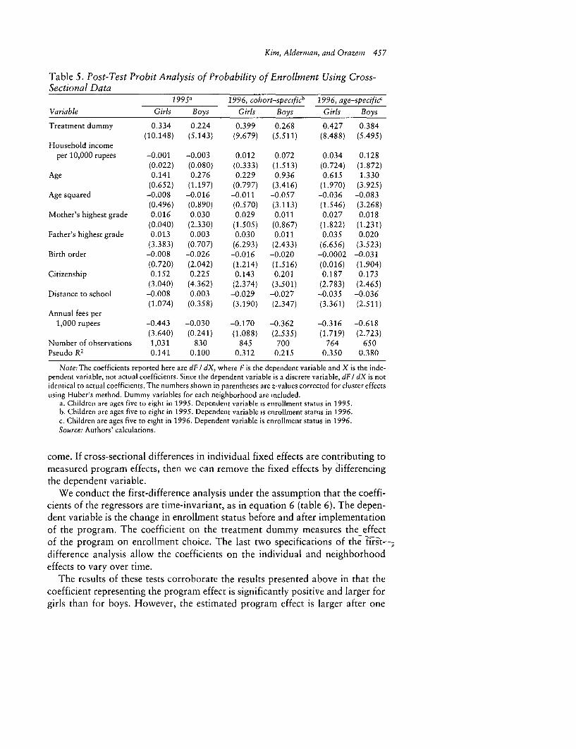
Kim, Aldermian, and Orazem 457
Table 5. Post-Test Probit Analysis of Probability of Enrollment Using Cross-Sectional Data
1995a 1996, cobort-spec,ficb 1996, age-specific'
Variable Girls Boys Girls Boys Girls Boys
Treatment dummy 0.334 0.224 0.399 0.268 0.427 0.384(10.148) (5.143) (9.679) (5.511) (8.488) (5.495)
Household incomeper 10,000 rupees -0.001 -0.003 0.012 0.072 0.034 0.128
(0.022) (0.080) (0.333) (1.513) (0.724) (1.872)Age 0.141 0.276 0.229 0.936 0.615 1.330
(0.652) (1.197) (0.797) (3.416) (1.970) (3.925)Age squared -0.008 -0.016 -0.011 -0.057 -0.036 -0.083
(0.496) (0.890) (0.570) (3.113) (1.546) (3.268)Mother's highest grade 0.016 0.030 0.029 0.011 0.027 0.018
(0.040) (2.330) (1.505) (0.867) (1.822) (1.231)Father's highest grade 0.013 0.003 0.030 0.011 0.035 0.020
(3.383) (0.707) (6.293) (2.433) (6.656) (3.523)Birth order -0.008 -0.026 -0.016 -0.020 -0.0002 -0.031
(0.720) (2.042) (1.214) (1.516) (0.016) (1.904)Citizenship 0.152 0.225 0.143 0.201 0.187 0.173
(3.040) (4.362) (2.374) (3.501) (2.783) (2.465)Distance to school -0.008 0.003 -0.029 -0.027 -0.035 -0.036
(1.074) (0.358) (3.190) (2.347) (3.361) (2.511)Annual fees per
1,000 rupees -0.443 -0.030 -0.170 -0.362 -0.316 -0.618(3.640) (0.241) (1.088) (2.535) (1.719) (2.723)
Number of observations 1,031 830 845 700 764 650Pseudo R2 0.141 0.100 0.312 0.215 0.350 0.380
Note: The coefficients reported here are dF I dX, where F is the dependent variable and X is the inde-pendent variable, not actual coefficients. Since the dependent variable is a discrete variable, dF / dX is notidentical to actual coefficients. The numbers shown in parentheses are z-values corrected for cluster effectsusing Huber's method. Dummy variables for each neighborhood are included.
a. Children are ages five to eight in 1995. Dependent variable is enrollment status in 1995.b. Children are ages five to eight in 1995. Dependent variable is enrollment status in 1996.c. Children are ages five to eight in 1996. Dependent variable is enrollment status in 1996.Source: Authors' calculations.
come. If cross-sectional differences in individual fixed effects are contributing tomeasured program effects, then we can remove the fixed effects by differencingthe dependent variable.
We conduct the first-difference analysis under the assumption that the coeffi-cients of the regressors are time-invariant, as in equation 6 (table 6). The depen-dent variable is the change in enrollment status before and after implementationof the program. The coefficient on the treatment dummy measures the effectof the program on enrollment choice. The last two specifications of the frst-difference analysis allow the coefficients on the individual and neighborhoodeffects to vary over time.
The results of these tests corroborate the results presented above in that thecoefficient representing the program effect is significantly positive and larger forgirls than for boys. However, the estimated program effect is larger after one

Table 6. First-Difference Probits for the Change in Enrollment Decision1994-95 1994-96 1994-1995 1994-96
Variable Girls Boys Girls Boys Girls Boys Girls Boys
Treatment dummy 0.367 0.292 0.264 0.088 0.469 0.428 0.281 0.242(5.518) (3.591) (3.165) (0.909) (5.833) (3.755) (2.931) (1.723)
Change in age squared -0.077 -0.082 -0.047 -0.046 -0.071 0.032 0.079 0.073(4.785) (4.447) (5.006) (4.502) (0.343) (0.137) (0.641) (1.323)
Age in 1994 squared -0.001 -0.022 -0.047 -0.080(0.040) (0.525) (1.055) (1.686)
Income per 10,000 rupees -0.151 -0.009 -0.009 -0.005(2.680) (0.122) (1.309) (0.588)
Mother's highest grade -0.007 0.016 -0.009 -0.030(0.374) (0.652) (0.380) (1.020)
Father's highest grade 0.004 -0.028 0.043 0.014(0.458) (2.751) (4.561) (1.226)
Birth order -0.029 -o.oso -0.008 -0.021(1.152) (1.667) (0.250) (0.616)
Citizenship 0.006 0.093 0.243 0.212(0.047) (0.717) (1.515) (1.318)
Distance to school -0.001 0.027 -0.054 0.029(0.051) (1.407) (1.936) (1.272)
Annual fees per 1,000 rupees -0.755 -0.103 -0.588 0.76s(2.424) (0.299) (1.623) (1.813)
Number of observations 1,055 861 863 725Pseudo R2 0.04 0.04 0.09 0.05
Note: The coefficients reported here are dF I dX, not actual coefficients. Children in the sample were ages four to seven in 1994.Source: Authors' calculations.

Kinm, Alderman, and Orazeem 459
year than after two years, in contrast to the cross-sectional results. The reasonfor this discrepancy is unclear, although it may be related to the fact that first-difference regressions control for fixed effects. Enrollment rates were initiallyhigher in the fellowship neighborhoods, and children who were in school beforethe fellowship schools opened do not contribute to the measured enrollment ef-fect in the first-difference analysis.
Also, the opening of the fellowship schools may have encouraged parents tosend their children to school at a younger age, and the smaller effect over timereflects the first-time enrollment of older children in the control neighborhoods.In fact, some of the later enrollment growth in control neighborhoods may havebeen related to the fellowship program if the promotion of children's educationin fellowship neighborhoods spilled over to control neighborhoods. Neverthe-less, the estimated two-year effect on enrollment growth is still large. Controllingfor fixed effects lowers the estimated effect 12 to 30 percent, leaving the esti-mated enrollment impact at 24.2 percent for boys and 28.1 percent for girls.
Given the apparent success of the fellowship schools in increasing enrollment,the question remains as to how much the children are learning. Assessment ef-forts are in their infancy in Balochistan, but the Balochistan Education Manage-ment Information System did pilot an achievement test to several third-gradeclasses, including some from fellowship schools. The results are not definitivebecause the samples were small, but they show no significant differences in out-come between fellowship and government schools. Still, any concrete assessmentof the relative quality of fellowship and government schools will require furthertests.
V. DISCUSSION
The fellowship program certainly increases enrollment. But is it cost-effectivewhen compared with alternative policy options? One way to look at this ques-tion is in terms of the cost per student enrolled. In 1996 the recurrent cost perstudent in government primary schools in Balochistan was 2,500 rupees (WorldBank 1997). This amount is nearly twice the subsidy per girl offered to the fel-lowship schools in the first year of operation and is far more than three times thesubsidy per student.13 The disparity is not due to cost recovery from students,since in the first year of operation students were asked to pay only between 10and 25 rupees per month. The difference comes mainly from lower teachersalaries.
In addition to these recurrent costs, the Primary Education Department spentapproximately 1,500 rupees per student in contracting a local NGO to help com-munities establish schools and train teachers. This amount also covered the moni-toring of schools during their first two years. Since the fellowship program did
13. Ideally, we would want to evaluate the cost of educating a student until graduation, but the projectis too new to ascertain this.

460 THE WORLD BANK ECONOMIC REVIEW, VOL. 13, NO 3
not build schools, these costs were its main start-up expenses. In the future NGO
costs will be lower, since the cost of monitoring activities necessary to conductthis evaluation will not be needed in expanding the pilot program. Nevertheless,even the upper-bound estimated start-up cost of 1,500 rupees per student is farless than the estimated cost of 600,000 rupees for the construction of a govern-ment primary school, which typically has two classrooms. Assuming 50 studentsper classroom, this represents an initial investment of 6,000 rupees per student.Thus there is a substantial difference in the cost of establishing a governmentschool relative to a fellowship school.
Instead of looking at the average cost per student, we can look at the marginalcost of increasing enrollment. We consider two alternative policies needed tomatch the enrollment increase that resulted from the fellowship program: in-come transfers to poor households and construction of new schools. Our esti-mates are based on estimated elasticities of enrollment choice with respect toincome and distance to school.
Income has only a moderate impact on participation in the program. Conse-quently, the benefits of the program are not strongly skewed to upper-incomehouseholds. The moderate income response also implies that it would take asizable income transfer to achieve the same impact on enrollment as the pro-gram. In particular, the income response in our estimates implies that a directsubsidy of 3,471 rupees per household would be needed to raise the probabilityof girls' enrollment 25 percent (table 7). This is roughly 2.5 times the initialrecurrent cost of a fellowship school-1,400 rupees a year per girl. As boys'enrollment is less income-sensitive, a similar increase in the probability of boys'enrollment would require an income transfer of 15,030 rupees, compared withthe negligible marginal cost of increasing boys' enrollment through the girls' fel-lowship program.' 4
The overall impact of the fellowship program might also be influenced by thefact that it reduces the distance to schools. Unfortunately, in our sample there isinsufficient variance in distance to schools to directly estimate this influence.Using the 1996 coefficient of distance for girls, -0.03 (see table 5), we estimatethat the distance to private schools would have to be cut in half to increase en-rollment by the same amount as the project. Halving the distance to schools in atwo-dimensional environment implies a fourfold increase in the number of schools.
An additional question is whether the success of the fellowship program de-pended on the attributes of the neighborhoods in which the new schools wereinstituted. There are large differences in success rates across neighborhoods, withthe increase in girls' enrollment varying from 8 to 67 percentage points. Increasesin boys' enrollment also differ across neighborhoods, from a drop of 2 percent-
14. The result for Quetta is similar to results for both sexes in low-income neighborhoods of Lahore,where a 10 percent increase in household income causes a 1.2 percent increase in the enrollment rate inprivate schools (Alderman, Orazem, and Paterno 1996). Thus in Lahore, a city in which overall primaryschool enrollment rates are more than 90 percent, an income transfer of 14,808 rupees would be requiredto raise enrollment 25 percent for both sexes.

Kmni, Alderman, and Orazenm 461
Table 7. Estimates of Alternative Ways to Raise Enrollmentto the Target Level
Change required toElasticities meet target level (25 percent)
Alternatives Girls Boys Girls Boys
Direct subsidy to household 0.503 0.115 3,471 rupees per 15,030 rupees perhousehold household(50 percent) (150 percent)
Decrease distance to school 0.320 0.732 13.48 minutes 5.71 minutes(78 percent) (34 percent)
Note: Children in the sample were ages 4 to 7. The numbers in parentheses are the amount as apercentage needed to meet target effect. For example, a direct subsidy to the household that leads to a 50percent increase in household income may raise girls' enrollment rates 25 percent.
Source: Authors' calculations.
age points to an increase of 61 percentage points. Are the fellowship schoolsmore successful in neighborhoods where households are not as poor, better edu-cated, or unique in other observable ways? For the most part success appears tobe unrelated to neighborhood attributes."5 The attributes of neighborhoods withabove-average enrollment gains do not differ much from those with below-average gains. For example, average parental education levels are similar in themost and least successful neighborhoods, and average income levels are actuallylower in the more successful neighborhoods. One intriguing result is that neigh-borhoods with the largest increases in girls' enrollment also have the largest in-creases in boys' enrollment, which is consistent with our presumption that boys'and girls' schooling are complementary goods.
To the extent that the schools benefit some types of children more or less thanothers, it appears that enrollment of younger children rises more than that ofolder children. This is a natural consequence of the fact that older children aremore likely to be at an age at which parents planned to remove them from schoolanyway. First-born children are more positively affected, presumably becauseparents favor the eldest child. Nevertheless, the joint test of uniform effects acrossall children cannot be rejected at standard significance levels, suggesting a highprobability of success from expanding the program to other poor neighborhoods,regardless of residents' socioeconomic attributes.
A final concern is whether these schools are sustainable. Ideally, we would liketo know if they will continue to operate for a generation or more. Unfortunately,we cannot answer this question given the time frame of our research. There are,however, encouraging indications that the program is viable. First, there is ademand for such schools from urban neighborhoods, including other cities in theprovince. The program has expanded from 11 schools with slightly more than2,000 students to 40 schools with 10,000 students. All of the schools that openedin urban areas between 1995 and 1998 remain open. Moreover, the enrollment
15. This discussion is based on Kim, Alderman, and Orazem (1998: 21-22, app. 3).

462 THE WORLD BANK ECONOMIC REVIEW, VOL. 13, NO. 3
of girls in the original schools covered in this study increased 15 percent between1996 (the last year in our household sample) and 1997, despite a nominal in-crease in fees of 15 percent-a small real increase of about 3 percent.16
Still, the schools are not financially independent. The Balochistan EducationFoundation provides about 20 percent of the subsidy given to these schools intheir first year of operation. This commitment-financed from an endowmentthat is distinct from the Primary Education Department's budget-may be in-tended to address the issue of equity. There is no direct indication that it is neededto ensure the viability of the schools.
VI. SUMMARY
We have used several evaluation methods based on experimental design tomeasure the effect of the Quetta Urban Fellowship Program on the enrollment ofboys and girls in poor neighborhoods. Regardless of how the impact is measured,we find that the fellowship program raised enrollment for both boys and girls(see table 3). Most estimates show that the effect was larger for girls than forboys. We can conclude that the estimated program effects are, robust to differ-ences in assumptions about possible biases arising from measured and unmea-sured differences between treatment and control neighborhoods.
Before the project was implemented, it was not clear whether girls' low en-rollment rates were due to cultural barriers that cause parents to keep theirdaughters out of school or to an inadequate supply of girls' schools. The urbanfellowship experiment provides strong evidence that subsidizing the establish-ment of primary schools for girls can sharply increase girfs' enrollment. In addi-tion, even though the fellowship was given only to girls, boys' enrollment inthose neighborhoods also increased sharply. This suggests that boys' educationand girls' education are complementary goods: by encouraging parents to sendtheir girls to school, the program had collateral benefits of raising boys' enroll-ment rates.
The measured change over two years yields mixed evidence on whether theadvantage for enrollment growth in fellowship neighborhoods relative to controlneighborhoods continued to increase. However, even if the initial enrollmentgain decreased in subsequent years, the increase in enrollment after two yearswas still around 25 percentage points. This is a substantial improvement over thebaseline enrollment rate of 45 percent for girls who are five to eight years old.School success appears not to depend on neighborhood income or other observ-able socioeconomic variables, suggesting that expanding the program to otherpoor neighborhoods is also likely to be successful.
Future work will be required to assess the long-term effects of the fellowshipprogram. In particular, the sustainability of the schools and the enrollment ef-
16. The school with the largest fee increase has the largest percentage increase in enrollment, perhapsreflecting the endogeneity of fee structures.

Kim, Alderman, and Orazem 463
fects after the subsidies expire must be evaluated. The short-term success of thefellowship program does not guarantee long-term success when the financialburden of supporting the schools is fully borne by the neighborhoods. Schooloutcomes must also be assessed. The ultimate success of the fellowship programdepends on whether children attain literacy.
APPENDIX. DETAILS ON THE ESTIMATES OF HOUSEHOLD INCOME
It is difficult to derive income estimates for households in Pakistan. The rela-tive importance of production for home consumption, informal labor marketarrangements, barter trade, and other economic activity occurring outside for-mal markets complicate efforts to measure income. The budget for this projectdid not include resources sufficient to carry out a careful analysis of income foreach household. However, the Pakistan Integrated Household Survey (PIHS) con-ducted such a detailed survey of household income and socioeconomic attributesin 1991. The PIHS allows us to predict household income based on a regression ofincome on easily observed household attributes. In this study we collected infor-mation on these attributes and then used the PIHS estimates to generate predictedincome.
The PIHS income equation is reported in table A-1. The specification followsAlderman and Garcia (1996), who estimate income and expenditure equationsfor 217 households in a single district in Balochistan. Their estimates can serveas independent validation of the income estimates we derive from the PIHS
data. They are less useful for our purpose than is the PIHS because their dataare from 1986 and include only rural households. The PIHS has sufficient ur-ban observations to estimate an income equation for urban households, and itis closer to our 1994 base period. The variables in the income equation includethe number of adult men and women, the number of men and women withprimary-, secondary-, and tertiary-level schooling, and the value of householdassets. Alderman and Garcia find that this income specification generates pre-dicted values that perform well in explaining household savings, loans, andnutrition status.
In general, the PIHS income estimates are sensible. Households with more capi-tal assets, more human capital, and more adult males have higher incomes. Theresults correspond reasonably well in sign with those in Alderman and Garcia.More important, the two studies generate equivalent estimates of relative house-hold income. The correlation in predicted income based on the PIHS comparedwith the Alderman-Garcia estimates is 0.82. The higher variance in income in thetreatment neighborhoods is a result of three wealthy households residing in thoseneighborhoods. When those households are removed, the treatment and controlneighborhoods have similar means and variances in estimated income.

464 THE WORLD BANK ECONOMIC REVIEW, VOL. 13, NO. 3
Table A-1. Income EquationsAlderman Pakistan Integrated
Variable and Garcia Household Survey
Intercept 5,999 3,303(2.61) (4.64)
Number of males ages 16 or older 938 1,219(0.92) (3.73)
Number of males ages 6-16 1,691(2.09)
Number of females ages 16 or more -709 -188(-0.54) (-0.57)
Number of females ages 6-16 1,009(0.64)
Number of children age 5 or younger 2,820(2.99)
Number of males with primary schooling 6,140 -1,171(2.95) (-2.55)
Number of males with secondary schooling 2,279 -364(1.69) (-0.92)
Number of males with more than secondary schooling 6,435 147(1.41) (0.96)
Number of females with primary schooling 6,707 -406(1.85) (-0.69)
Number of females with middle schooling or more 7,758 889(1.35) (3.68)
Rainfed land 110 n.a.(2.34)
Irrigated land 665 n.a.(4.93)
Acres of orchards 4,065 n.a.(2.57)
Value of livestock 0.335 n.a.(1.05)
Value of vehicles 0.171 0.012(8.55) (2.48)
Value of machinery and tools 0.125 0.007(1.27) (1.88)
R2 0.747 0.03Number of observations 217 2,112
- Not available.n.a. Not applicable.Note: Numbers in parentheses are standard errors.Source: Authors' calculations.
REFERENCES
The word "processed" describes informally reproduced works that may not be com-monly available through library systems.
Alderman, Harold, Jere Behrman, David Ross, and Richard Sabot. 1996. "Decomposingthe Gender Gap in Cognitive Skills in a Poor Rural Economy." Journal of HumanResources 32(1):229-54.

Kim, Alderman, and Orazem 465
Alderman, Harold, and Marito Garcia. 1996. Poverty, Household Food Security, andNutrition in Rural Pakistan. Research Report 96. Washington, D.C.: InternationalFood Policy Research Institute.
Alderman, Harold, and Elizabeth King. 1998. "Gender Differences in Parental Invest-ment in Education." Structural Change and Economic Dynamics 9(4):453-68.
Alderman, Harold, Peter Orazem, and Elizabeth M. Paterno. 1996. "School Quality,School Cost, and the Public/Private School Choices of Low-Income Households inPakistan." Impact Evaluation of Education Reform Working Paper 2. World Bank,Development Research Group, Washington, D.C. Processed.
Becker, Gary S. 1981. A Treatise on the Family. Cambridge, Mass.: Harvard UniversityPress.
Behrman, Jere, and Anil Deolalikar. 1995. "Are There Differential Returns to Schoolingby Gender? The Case of Indonesian Labor Markets." Oxford Bulletin of Economicsand Statistics 57(1):97-117.
Butcher, Kristen, and Anne Case. 1994. "The Effect of Sibling Sex Composition onWomen's Education and Earnings." Quarterly Journal of Economics 109(3):531-62.
Grossman, Jean Baldwin. 1994. "Evaluating Social Policies: Principles and U.S. Experi-ence." The World Bank Research Observer 9(2):159-80.
Kim, Jooseop, Harold Alderman, and Peter Orazem. 1998. "Can Private School Subsi-dies Increase Schooling for the Poor? The Quetta Urban Fellowship Program." ImpactEvaluation of Education Reforms Working Paper 11. World Bank, Development Re-search Group, Washington, D.C. Processed.
Newman, John, Laura Rawlings, and Paul Gertler. 1994. "Using Randomized ControlDesigns in Evaluating Social Sector Programs in Developing Countries." The WorldBank Research Observer 9(2):181-201.
Parish, William, and Robert Willis. 1993. "Daughters, Education, and Family Budgets:Taiwan Experiences." Journal of Human Resources 28(4):863-98.
Schultz, T. Paul. 1995. Investment in Women's Human Capital. Chicago: University ofChicago Press.
World Bank. 1997. "Pakistan: Toward a Strategy for Elementary Education." Report16670-PAK. World Bank, South Asia Region, Washington, D.C. Processed.


THE WORLD BANK ECONOMIC REVIEW, VOL. 13, NO. 3: 467-91
Central Mandates and Local Incentives:The Colombia Education Voucher Program
Elizabeth M. King, Peter F. Orazem, and Darin Wohlgemuth
In decentralized education systems programs that promote central mandates may haveto be devolved to local governments, communities, and providers. When participationby local governments and providers is voluntary rather than compulsory, the determi-nants of program placement are important in predicting potential benefits to individu-als. This article analyzes incentives for municipalities and private schools to participatein Colombia's voucher program. It finds that the demand for secondary education rela-tive to the capacity of public schools and the availability of spaces in private schools inthe municipality were key predictors of municipal participation, whereas the number ofunderserved students had a nonlinear effect on participation. Schools whose educationalquality was moderate and charged moderate tuition fees were the most likely to partici-pate; the program was less attractive to schools whose quality and fees were high and toschools whose quality and fees were low.
The debate regarding the use of vouchers for private schools, whether in indus-trial or developing countries, centers on issues of equity and efficiency (seeLevin 1991, 1992; Henig 1994; and CERI, OECD 1994 for a summary of thearguments). Proponents claim that vouchers provide the poor with a way outof overcrowded or low-quality schools by allowing them to enroll in privateschools that they would otherwise not be able to attend. Furthermore, if com-petition for voucher students impels both private and public schools to im-prove, then vouchers make the delivery of education per public dollar spentmore efficient.' Proponents also see vouchers as a means of transferring somecontrol over educational resources from the central or local government to par-ents and students. In countries where educational policy decisions are heavily
1. Moreover, there is consistent evidence that children perform better in private schools than in publicschools in developing countries, even when accounting for selection. See Jimenez, Lockheed, and Paqueo(1991) and Lockheed and Jimenez (1994) for reviews of this literature.
Elizabeth M. King is with the Development Research Group at the World Bank, and Peter F. Orazemand Darin Wohlgemuth are with the Department of Economics at Iowa State University. The authors' e-mail addresses are [email protected], [email protected], and [email protected]. The authors are gratefulto Marybell Gutierrez, Martha Laverde, Carlos Pardo, Laura Rawlings, Carlos Torres, and Fabio SanchezTorres for assistance in locating and accessing data. They also thank the referees for numerous helpfulcomments and suggestions, Berk Ozler and Dan Levy for expert assistance in organizing the data, andDonna Otto and Diana McLaughlin for preparing the manuscript. This study was funded jointly by theWorld Bank's Development Research Group and Research Support Budget under RPO 679-18.
C) 1999 The International Bank for Reconstruction and Development/THE WORLD BANK
467

468 THE WORLD BANK ECONOMIC REVIEW, VOL. 13, NO. 3
centralized, vouchers represent a dramatic shift in the locus of decisionmaking,with great potential to improve efficiency.
Opponents counter that vouchers rob public schools of much-needed resources,that vouchers are used by richer students who would have paid for private schoolanyway, and that private schools can pick and choose among students, leavingpublic schools with the worst students. Winkler and Rounds (1993) find thatparents select private schools based on the characteristics of the students alreadyenrolled. As a result private schools tend to have a continuing advantage in at-tracting students with higher socioeconomic status. Opponents also counter thatunless an efficient information system is developed to publicize the relative qual-ity of different private schools, parents and students will make uninformedchoices-a situation not likely to induce schools to improve their performance.
These efficiency issues are important for assessing the role of vouchers in in-dustrial countries; however, they may be only secondarily so in developing coun-tries, where the education choice is not whether to attend public school or pri-vate school, but whether or not to attend school at all, given the absence of anearby school. Expanding access to any school-not widening the choice ofschool-is probably the best argument in favor of vouchers in these countries.Partnerships with the private sector, which could lead to huge gains in enroll-ment, are a pragmatic response to strained or inadequate public school capacity,especially in poor rural areas or in overpopulated cities. High population growthrates will only exacerbate the problem over time. Without private schools, manychildren will not be able to attend school at all. Indeed, the proportion of second-ary students in private schools in developing countries is roughly double the me-dian in industrial economies (James 1993).
Previous research on vouchers has concentrated almost exclusively on evalu-ating the benefits of giving parents and students greater choice by comparingstudents' performance in public and private schools. Witte's (1996) review of theliterature contends that there is no evidence of increased achievement in privateschools, once we control for private schools' nonrandom selection of studentswith potentially higher abilities. In fact, Hoxby (1996), simulating the effect ofvouchers on student achievement, argues that vouchers would improve test scoresaveraged across all schools, but would lower test scores in private schools. Aver-age scores would rise because of improved public school efficiency, necessitatedby greater competition for students. However, Murnane, Newstead, and Olsen(1985), Sander (1996), Neal (1997), Sander and Krautmann (1995), and Witte(1996) find that attending Catholic school improves student achievement, evenafter controlling for selection, and raises the probability of attending college.Hoxby's (1996) and Lankford and Wyckoff's (1992) simulations based on schoolchoice models predict that vouchers would increase private school enrollment,but would not affect private school students who were poor or whose parentshad less education.
The evaluation of Chile's voucher program, one of the oldest voucher pro-grams in the developing world, has been the subject of debate as well. Winkler
King, Orazem, and Wohlgemuth 469
and Rounds (1996) and Gauri (1998) find that students with higher socioeco-nomic status were significantly more likely to enroll in better-performing schoolsthan were students from lower-income families. Rodriguez (1988, as cited byGauri) concludes that private subsidized or voucher schools in Santiago outper-formed the public centralized schools that still existed at that time. Parry (1993,as cited by Gauri) regresses schools' average scores in a national standardizedtest on average characteristics of the students and finds that, although municipalschools scored higher than voucher schools when parents had relatively littleeducation, voucher schools scored higher when parents were relatively moreeducated.
This research, however, generally ignores the supply response of providers,assuming that students are able to find space in a private school with attributesequal to those of the average private school. In reality, private schools may refuseto participate in a voucher program, as may local school boards, if participationis voluntary. Hence, the subset of participating providers may differ significantlyfrom the full population of.private schools. The potential benefits of the pro-gram, whether in terms of enrollment or student learning, will then depend onthe willingness of local communities and schools to participate. 2
In this article we examine the extent to which a central government is able toattain a national goal of expanding enrollment, especially among the poor, evenas it transfers power to local governments and private providers. Voluntary pro-gram participation and cost-sharing schemes between the central governmentand local governments are gaining currency in developing countries and areconsistent with shifts toward more decentralized delivery systems. We studyColombia's national voucher program for secondary education, which the gov-ernment launched in late 1991 and terminated in 1997.
True to Colombia's broad decentralization reforms of the early 1990s(Montenegro 1995; Hanson 1995), municipalities and schools participated inthis voucher program voluntarily, and municipalities assumed part of the cost ofthe program. Two key assumptions of the program were that public schools,especially those in large cities, were overcrowded and that private schools hadexcess capacity. Vouchers for use in private schools were viewed as a means toexpand enrollment in secondary schools at relatively low cost, while reducing the
2. The absence of a broad-based voucher program has made it impossible to estimate the supplyresponse of private schools and municipalities to such a system. Witte (1996: 170) argues, 'Nearly allquantitative estimates of [voucher effects onl school selection and the effects of school choice on performanceare based on extrapolations from the current system of education. However, a broad based voucher system... might create such a different market for education that estimates based on the current arrangementswould be meaningless."
To develop reasonable estimates of the effects of a voucher program, it is important to observe howschools respond to the existence of a voucher program, but "current experiments with vouchers ... aresimply too small to provide evidence of market reactions by either the public or private sectors" (Witte1996: 172). Witte contends that the crucial information on how schools respond to vouchers will beavailable only when a large-scale voucher program is implemented. Until then, researchers will not be ableto establish the validity of simulations based on existing schools.

470 THE WORLD BANK ECONOMIC REVIEW, VOL. 13, NO. 3
enrollment pressure on public schools.3 In addition, encouraging more privateprovision without directly subsidizing specific schools was seen as a way to elicitbetter performance from private schools. Vouchers could also improve the qual-ity of public schools by reducing overcrowding, thereby easing the pressure onresources in public schools.
We examine whether the decision of municipalities and private schools toparticipate in Columbia's voucher program was consistent with stated nationalobjectives. In particular, did municipalities' excess demand for secondary edu-cation or private schools' desire to reach poorer households significantly influ-ence participation?
I. COLOMBIA'S VOUCHER PROGRAM
Colombia launched its national voucher program near the end of 1991 as partof a broader transformation, begun in the late 1980s, to decentralize the organi-zation and management of its education system. Hanson (1995) traces the impe-tus for decentralization to the growing awareness among Colombia's elite of theneed to establish the legitimacy of the government and its institutions as a meansto deal with the country's increasing violence. The strategy for establishing legiti-macy hinged on giving people participatory control over public institutions. Bythe late 1980s several government institutions, including the educational system,had begun to decentralize. The new constitution of 1991 codified and integratedthese initiatives.
Together with other reforms, the voucher program was meant to address defi-ciencies in the performance of the public education system, especially the lowtransition rate from.primary to secondary school among the poor. In 1992 only51 percent of 13-19-year-old urban youths belonging to the poorest quintilewere enrolled in school, compared with 75 percent of those in the richest quintile(World Bank 1994). The shortage of space in public schools, especially in largecities, where demand was thought to be greatest, was seen as a real problem.
The Ministry of Education initially targeted the country's 10 largest cities forparticipation in the program. Adoption was ultimately voluntary, although theMinistry may. have pressured cities to join. In 1991 the Ministry of Educationheld a meeting with the heads of departments (states) to announce the program.The meeting elicited subsequent letters of intention to participate from depart-ments and municipalities, as well as statements about which municipalities werenot able or likely to join. The program grew nationally and during its most activeyear, 1995, had 217 participating municipalities in 27 of the country's 30 depart-ments. In 1995 the government awarded about 90,000 vouchers to students in1,800 private schools. Voucher students made up 8 percent of all students in
3. Limited evidence supports the conclusion that vouchers raise enrollment. Ribero and Tenjo (1997)find that in Bogota, where there were too few vouchers to meet demand, enrollment rates for students whoreceived vouchers were 12 percentage points higher than for students who qualified for but did not receivevouchers.
King, Orazem, and Wohlgemuth 471
private secondary schools. Student applicants had to have graduated from pri-mary school (completed fifth grade) and been admitted to a participating privateschool. Awardees could renew their vouchers in the subsequent year only if theywere promoted to the next grade. Dropouts and repeaters automatically lost theirvouchers.
Although participation in the program was widespread, most of the voucherswere issued in large urban areas, where private schools are concentrated. Tendepartments absorbed more than 70 percent of all vouchers issued, with the capi-tal city of Bogota alone taking 13 percent. 4 Participation was contingent on themunicipality's willingness to cofinance and administer the program. The munici-pality provided 20 percent of the funds for the vouchers issued in its area, and thecentral government provided the remaining 80 percent. 5
By design, Colombia's program avoided two common criticisms of voucherprograms. First, the program did not threaten the resources available to existingpublic schools. The government assured public schools that current levels of fund-ing would not decrease. This promise eliminated competition over finances, al-though public and private schools still had to compete for voucher students,especially because municipalities were able or willing to fund only a limited num-ber of vouchers. In fact, each year the demand for vouchers exceeded the supplyin nearly all participating municipalities. Conversations with officers from theadministering agency, the Colombian Institute for Education Credit and Train-ing Abroad (ICETEX), suggested that anywhere from 20 percent (in the depart-ment of Atlantico) to 90 percent (in Antioquia) of qualifying applicants receivedvouchers. In many cases where supply exceeded demand, a lottery was used toselect beneficiaries. Because this lottery randomized the selection of students forthe program, it provided a valuable mechanism for assessing the program's im-pact on individual students. Angrist and others (1999) examine this.
Second, only the poor qualified for vouchers, countering the claim that vouch-ers amount to a net subsidy for the wealthy at the expense of the poor. Thetargeting criterion used was based on a neighborhood stratification scheme thatranks neighborhoods on a scale of 1-6, from poorest to richest. A national pov-erty map, derived from five poverty indicators and used to distribute other trans-fers, established the socioeconomic status of different neighborhoods.6 Only stu-
4. See King and others (1997) for more details about the program.5. The agreement included additional conditions that did not relate directly to the program but were
part of the decentralization reform. Municipalities had to agree to the terms of Law 160, which transferredresponsibility for maintaining public schools from the central to the municipal government, and had to
maintain a system of accounts that satisfied nationally prescribed standards.6. The poverty map index, Necesidades Bdsicas Insatisfechas, was computed on the basis of five
indicators: the proportion of households living in inadequate homes (such as homes without walls), theproportion of households without an adequate water supply or sanitation services, the proportion ofhouseholds living in overcrowded quarters (defined as an average of more than three people per room), theproportion of households with high economic dependency (defined using the ratio of all household membersto employed household members and the educational attainment of the household head), and the proportionof households with children between the ages of 6 and 12 years who were not enrolled in school (Colombia,Department of National Planning 1994).

472 THE WORLD BANK ECONOMI4C REVIEW, VOL 13, NO. 3
dents residing in neighborhoods ranked 1 or 2 were eligible to receive a voucher.Morales-Cobo (1993) and Ribero and Tenjo (1997) conclude that the program'sgeographical targeting mechanism was accurate in delivering vouchers to poorstudents.7 In order to establish a student's socioeconomic status, and thus eligi-bility, the program required that each applicant present a national identificationcard or utility bills to verify residence.
The voucher covered the cost of tuition-the yearly entrance fee plus monthlyfees-for students in sixth to eleventh grade, subject to an upper limit. ICETEX,
which administered the program for the Ministry of Education, set the maximumvalue of the voucher each year. In 1995 the voucher was worth a maximum valueof Col$145,307 (Colombian pesos) or about $180 (U.S. dollars), with the actualvalue of each voucher depending on the prevailing tuition fee in the school inwhich the voucher was to be used.8 This upper limit met or exceeded the annualfees of lower-priced schools, but covered less than half of the cost of the highest-priced schools.
Since the voucher did not make all private schools affordable to poor parents,interest was greatest in the lower-cost schools. In our sample of schools the vouchercovered only one-fifth of the annual fees of the highest-priced private school. Intheory, parents could have used the voucher to pay for part of the fee and paidthe balance themselves. However, ICETEX administrators discouraged this prac-tice, fearing that private schools might raise their fees in response, thus transfer-ring part of the effective subsidy from the students to the schools.
II. MUNICIPAL PROGRAM PARTICIPATION
In this section we introduce a model that estimates the probability that amunicipality will participate in the voucher program. Underlying the model is theassumption that the municipality is responsible for providing secondary school-ing, subject to a fiscal constraint. To fulfill this responsibility, the municipalitycan build public schools or subsidize private schools.
In 1991 Colombia's central government transferred the responsibility for main-taining school facilities to departments and municipalities (Hanson 1995). Eachmunicipality thus inherited a supply gap in secondary schooling, which we callunderserved students, Su = SD - SS, where SD is demand for secondary schooling
7. Morales-Cobo (1993) finds that, at least in Bogota, the program reached its intended beneficiaries.Ribero and Tenjo (1997) find similar success, except that students in neighborhoods ranked 3 received 9-17 percent of the vouchers, depending on the particular municipality. Because residents of theseneighborhoods still had below-average incomes, Ribero and Tenjo confirm that the program was relativelywell targeted. Under this system of geographical targeting, leakage to unintended beneficiaries is likely,since low-income neighborhoods may have better-off residents. The higher cost of finer targeting, however,justifies a certain degree of leakage.
8. The voucher's maximum value was adjusted annually according to the estimated national inflationrate. The same adjustment was made to the voucher for each participating school, irrespective of changesin fees in those schools. In 1994, for example, the mean value of the voucher ranged from Col$59,700 inthe department of Choco to Col$119,100 in Quindio.
King, Orazem, and Wohlgemuth 473
and Ss is the sum of secondary enrollment capacity in public and private schools.If Su < 0, then secondary schooling capacity exceeds demand, and there is noneed to expand supply. If Su > 0, then the municipality must decide how to ex-pand secondary school capacity, conditional on having the funds to finance thatexpansion. 9
Model
If the municipality chooses to participate in the voucher program, it faces acost, v, per student for the voucher plus administration and advertising costs ofa(t) per student. We assume that these administrative and advertising costs de-crease in the taste for private school, t, because there would be less need to moti-vate parents of underserved students to participate in the voucher program ifthere were a strong tradition of private education in the municipality. As analternative to the voucher system, the municipality has the option of increasingpublic school capacity.10 This strategy has very high fixed costs relative to thevoucher program. However, as the number of underserved students increases,the average cost of this option, C(Su), declines. If it falls below v + a(t) over therange (0, Su), the municipality's cost-minimizing choice would be to increasepublic school capacity.
The municipal choice is illustrated in figure 1. Assume initially that the aver-age cost of providing a voucher is v + a(to). The average cost of expanding publicschool capacity is given by C(Su). If the number of underserved students is posi-tive but below Sou, and there is no capacity constraint on private schools, themunicipality will opt for the voucher program, it being the least-cost means ofadding secondary school capacity. Beyond So and up to Sb , the municipality willreject the voucher program in favor of providing additional space in public schools.But municipal choices are not limited to one or the other. If Su > Sb , the munici-pality will provide more public schools up to capacity Su and then vouchers forSu - Su
Thus far we have assumed that the municipality knows v + a(t) and C(Su) withcertainty. More realistically, there will be uncertainty regarding the average costof expanding capacity. Let uv be a random additive error to the average cost ofthe voucher, and let uc be a random additive error to the average cost of schoolconstruction. Let VG be the number of vouchers issued by the municipal govern-ment. The probability that the municipality will participate in the voucher pro-gram is
(1) P(VG > 0) = P[(SU > 0) A ([v + a(t) - C(Su)] < (u, - uv)l]
9. Ministry of Education and departmental officials informed us that the central government hadtargeted some municipalities for participation, but targeted municipalities could and did turn down theinvitation. Furthermore, municipalities that the central government did not target could and did enter theprogram. Therefore, it is reasonable to model municipal choice as a local decision.
10. Of course, municipalities could reject vouchers and any other role in secondary education. Thusmunicipalities that opted not to participate in the voucher program did not necessarily expand secondaryschool capacity by other means.
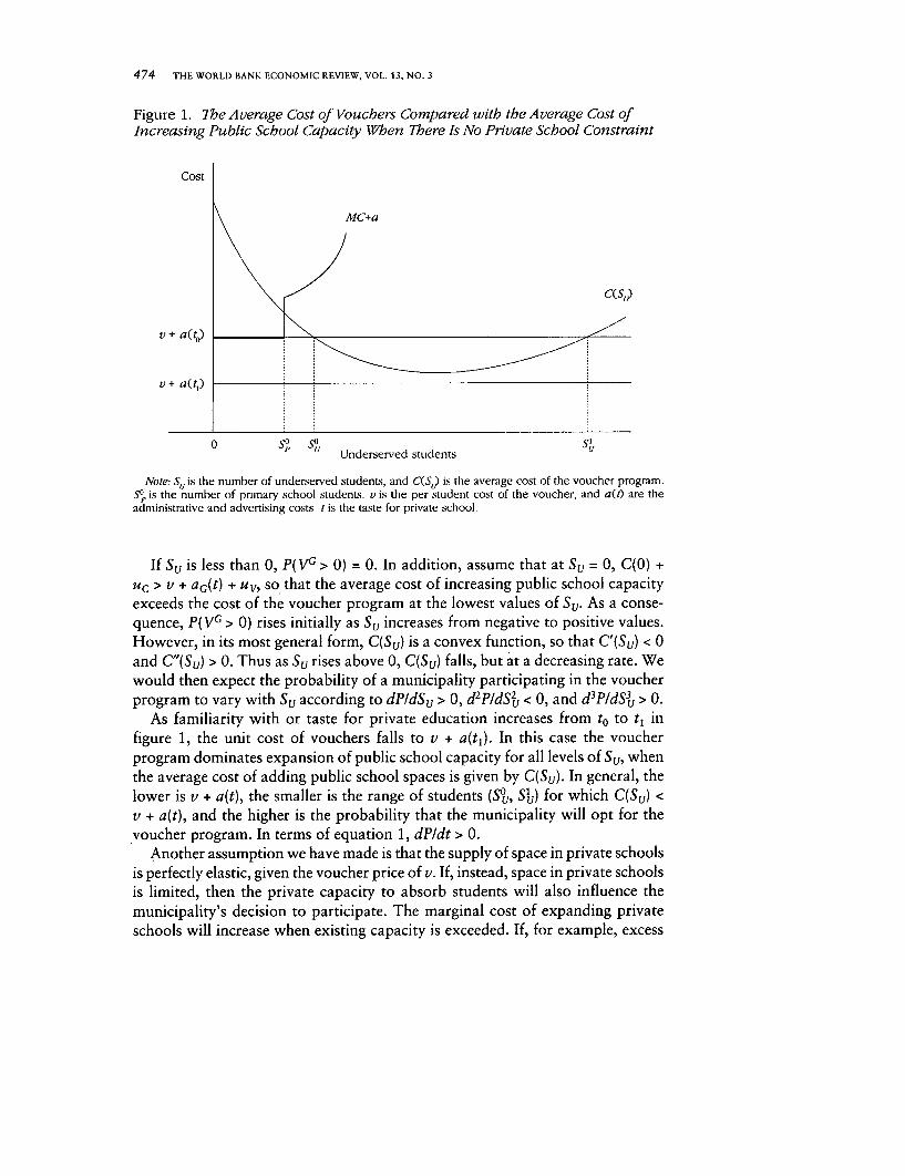
474 THE WORLD BANK ECONOMIC REVIEW, VOL. 13, NO. 3
Figure 1. The Average Cost of Vouchers Compared witb the Average Cost ofIncreasing Public School Capacity When There Is No Private School Constraint
Cost
MC+a
C(S,)
v+ a(t)
v + a(t)
O Underserved students SI1
Note: -Suis the number of underserved students, and C(S5) is the average cost of the voucher program.5sp is the number of primary school students. v is the per student cost of the voucher, and a(l) are theadministrative and advertising costs t is the taste for private school.
If Su is less than 0, P(VG > 0) = 0. In addition, assume that at Su = 0, C(0) +UC > v + aG(t) + uv, so that the average cost of increasing public school capacityexceeds the cost of the voucher program at the lowest values of Su. As a conse-quence, P(VG > 0) rises initially as Su increases from negative to positive values.However, in its most general form, C(Su) is a convex function, so that C'(Su) < 0and C'(Su) > 0. Thus as Su rises above 0, C(Su) falls, but at a decreasing rate. Wewould then expect the probability of a municipality participating in the voucherprogram to vary with Su according to dPIdSu > 0, d2PIdS2 < 0, and d3 PldS3 > 0.
As familiarity with or taste for private education increases from to to t1 infigure 1, the unit cost of vouchers falls to v + a(tl). In this case the voucherprogram dominates expansion of public school capacity for all levels of Su, whenthe average cost of adding public school spaces is given by C(Su). In general, thelower is v + a(t), the smaller is the range of students (SO , SIb) for which C(Su) <v + a(t), and the higher is the probability that the municipality will opt for thevoucher program. In terms of equation 1, dPldt > 0.
Another assumption we have made is that the supply of space in private schoolsis perfectly elastic, given the voucher price of v. If, instead, space in private schoolsis limited, then the private capacity to absorb students will also influence themunicipality's decision to participate. The marginal cost of expanding privateschools will increase when existing capacity is exceeded. If, for example, excess

King, Orazem, and Wohlgemuth 475
capacity of existing private schools is Sp, the supply curve will have a discontinu-ous jump at that point, and the number of vouchers offered by the municipalitywill be less than if supply were perfectly elastic. Therefore, if Sp is excess capacityin existing private schools, we expect dPIdSp > 0.
We have also assumed thus far that municipalities do not face budget con-straints. However, as a condition of participation, municipalities had to demon-strate that they had the fiscal capacity to take over the maintenance of publicschools. Municipalities with little ability to raise public revenues, B, would beconstrained from participating, so that dP/dB > 0.
The model of a municipality that minimizes costs suggests that the probabilityof participation in the voucher program as defined by equation 1 can be opera-tionalized as:
(2) P(VG > 0) = f[C(SU), Sp, t,B, v, £]+ + + + _
where E = Uc - UV, and the expected signs of the partial derivatives of P(VG > 0)with respect to the explanatory variables are indicated.
Data
We estimate equation 2 using data for 923 municipalities in Colombia,208 (or 23 percent) of which opted to participate in the program. The 923represent all of the municipalities in the 28 of 30 departments for which wehad the necessary data. We collected program administrative data from ICETEX
central and regional offices over 1995-97, and we found data on the charac-teristics of municipalities from other existing databases (table 1). Since thevariables that we are treating as exogenous in the equation could themselveschange in response to a municipality's decision to participate or not in theprogram, we measure all such variables as of 1991, before the voucher pro-gram was implemented.
The number of underserved students is the difference between the number ofprimary school students, S- 5, and the number of secondary school students,S6-11, measured before implementation of the voucher program. Given the goalof universal secondary enrollment, primary enrollment measures the populationof potential secondary students. The total number of private and public second-ary school students is a measure of existing secondary school capacity. We dividethe difference between the number of potential secondary school students andthe number of current secondary school students by the number of public sec-ondary school teachers. This measure suggests how many additional studentswould need to be placed per public classroom in order to cover all potentiallyunderserved students. The resulting measure is
(3) Su = - S

476 THE WORLD BANK ECONOMIC REVIEW, VOL. 13, NO. 3
Table 1. Sample Statistics for Participating and NonparticipatingMunicipalitiesVariable Total Nonparticipants Participants
Endogenous variableParticipation decision 0.22 0 1
(0.41)Exogenous variablesUnderserved students (SU)a 12.16 11.27 15.31
(24.84) (23.60) (28.65)Basic needs index (N) 0.60 0.63 0.51
(0.21) (0.20) (0.20)Underserved students interacted with basic
needs index (Su * N) 8.03 7.72 9.14(17.93) (17.64) (18.93)
Ratio of secondary private teachers toprimary students 0.0052 0.0025 0.015
(0.012) (0.0097) (0.015)Proportion of private primary students 0.052 0.028 0.14
(0.10) (0.07) (0.13)Per capita taxes paid (Col$10,000) 0.29 0.22 0.44
(0.67) (0.39) (0.66)Proportion of primary schools that are rural 0.30 0.31 0.29
(0.34) (0.35) (0.31)
General informationPupil-teacher ratio
Private secondary 15.16 13.06 16.42Public secondary 18.46 17.49 21.90
Number of studentsPrimary 3,537 1,131 12,107Secondary 3,022 792 10,963
Number of municipalities 923 715 208
Note: Values given are means. Standard deviations are in parentheses.a. Underserved students = (number of primary students - number of secondary students)/number of
secondary public teachers.Source: Authors' calculations based on program administrative data from ICETEX central and regional
offices, 1995-97, and SABER data, 1992-93.
where r6-11 is the number of full-time public secondary school teachers. Largervalues of Su will make it harder for existing public schools to absorb the addi-tional students. Consistent with that presumption, measured Su was 36 percenthigher in participating than in nonparticipating municipalities.
Because vouchers were targeted toward poor students, we use the basic needsindex (see footnote 6). This index, N, measures the proportion of the municipalpopulation that is considered poor according to five different poverty indicators.Fifty-one percent of the population in participating municipalities was consid-ered poor, compared to 63 percent in nonparticipating municipalities.
It is possible that existing public schools may have been to provide spaces forpoor children in some municipalities. Thus we interact N with Su to generate aproxy measure of needy underserved students per public secondary school teacher.This measure is 18 percent higher on average in participating than in nonpartici-

King, Orazem, and Wohbgemuth 477
pating municipalities. Consequently, before the voucher program began, partici-pating municipalities had a smaller proportion of needy households but a largerproportion of needy underserved students relative to existing public schoolcapacity.
We measure the capacity of private schools to absorb additional students byT6-11 / S1-5, where Tp1 I is the number of secondary school teachers (and, presum-ably, classrooms) in existing private schools. Before the voucher program wasestablished, this ratio was six times higher in participating than in nonparticipat-ing municipalities. In addition, the proportion of primary school students in pri-vate school was 0.14 in participating municipalities, five times higher than theproportion in nonparticipating municipalities.
We use two measures of government capacity to raise revenue. The first is theproportion of poor people in the municipality, as measured by the needs index.Poorer municipalities have less capacity to raise revenue, although the averagepoverty indexes for participating and nonparticipating municipalities were virtu-ally identical. The second measure is 1991 per capita income taxes paid in themunicipality. This was two times higher in participating than in nonparticipatingmunicipalities. Participating municipalities also had larger populations of schoolchildren. Primary enrollment was nearly 11 times higher in participating munici-palities. However, the proportion of rural schools, as designated by the Ministryof Education, was nearly identical across the two groups.
Estimation and Results
The most important parameters in the probit model of voucher participation(equation 2) pertain to the measure of underserved students (table 2). We expectSu to affect participation in a nonlinear fashion, initially raising and then lower-ing the probability of participating. We first include a cubic form of Su. Althoughthe sign pattern corresponds to our expectations, the third-order term is not sig-nificant. The results reported in table 2 use a quadratic approximation of Su. Atsample means the marginal effect of this variable is positive. The elasticity im-plies that a 10 percent increase in the number of underserved students per sec-ondary school teacher would increase the probability of municipal participationby 2.8 percent.
We also trace out the nonlinear effect of Su using a spline function. The coef-ficients on the dummy variables representing whether the measure of underservedstudents was positive, in the upper 50 percent, upper 30 percent, upper 20 per-cent, and upper 10 percent of the distribution of Su or NSu are cumulative (col-umns 2 and 4 of table 2).11 That is, other things constant, the total effect of beingin the upper 30 percent of the distribution of Su is the sum of the coefficients on
11. Municipalities that attracted students from surrounding towns show negative values of SU. Thedistributional information on Su and NS, (table 1) shows that they both turn positive at the thirtiethpercentile, so the first dummy variable represents the upper 70 percent of the distribution of underservedstudents.

478 THE WORLD BANK ECONOMIC REVIEW, VOL. 13, NO. 3
Table 2. Probit Estimates for Municipal Participation in the Voucher ProgramVariable 1 2 3a 4a
SU/100 1.779*** 2.667***(3.800) (3.503)[0.285] [0.285]
(SU/100)2 -0.743*** -1.600**(-2.436) (-2.277)
SU>2 0 -0.0288 -0.034(-0.174) (-0.206)[-0.001] [0.0004]
Municipality is in the fiftiethpercentile of Sudistribution 0.327 0.368
(1.900) (2.109)[0.040] [0.239]
Municipality is in the seventiethpercentile of S. distribution 0.268 0.249
(1.360) (1.262)[0.066] [0.0371
Municipality is in the eightiethpercentile of Sudistribution 0.196 0.103
(0.922) (0.472)[0.075] [0.025]
Municipality is in the top ninetiethpercentile of Su distribution -0.105 0.058
(-0.486) (0.262)[-0.082] [-0.0311
Secondary private teachers/primarystudents/100 0.342*** 0.341*** 0.341*** 0.343**
(8.718) (8.651) (8.691) (8.687)[0.265] [0.264] [0.264] [0.268]
Proportion of private primary students 4.091*** 4.011*** 4.061*** 4.006***(7.476) (7.291) (7.384) (7.251)[0.315] [0.309] [0.313] [0.311]
Proportion of primary schoolsthat are rural -0.125 -0.161 -0.093 -0.124
(-0.634) (-0.797) (-0.481) (-0.633)[-0.056] [-0.072] [-0.042] [-0.056]
Per capita taxes paid (Col$10,000) 0.0363 0.0566 0.0272 0.024(0.448) (0.640) (0.340) (0.296)[0.015] [0.024] [0.012] [0.010]
Needs index -0.966* * -0.960*** -1.224*v* -1.368***(-3.642) (-3.577) (-4.278) (-4.445)[-0.856] [-0.853] [-1.087] [-1.222]
Constant -0.87** * -0.963** -0.716** -0.736* * *(-4.856) (-4.732) (-3.837) (-3.315)
Sample size 923 923 923 923Log-likelihood -358.097 -355.594 -358.196 -355.195Pseudo R-squared 0.2729 0.2780 0.2727 0.2766
** Significant at the 5 percent level.Significant at the 1 percent level.
Note: S., the number of underserved students, equals (number of primary students - number of secondarystudents)/number of secondary public teachers. z-statistics are in parentheses. Elasticities are in bracketsand are computed at the median of the range for the dummy variables.
a. Su is interacted with the needs index.Source: Authors' calculations based on program administrative data from ICETEX central and regional
offices, 1995-97, and SABER data, 1992-93.

King, Orazem, and Wohlgemuth 479
Su when Su is positive, in the upper 50 percent of the distribution, and in theupper 30 percent of the distribution. The results suggest a rising probability ofparticipation between the fiftieth and ninetieth percentiles.
The relationship between P(VG > 0) and Su as captured by the equations incolumns 1 and 2 are shown in figures 2 and 3. In the quadratic representation(figure 2) the probability rises throughout the sample range of underserved stu-dents. The spline function (figure 3) peaks at just over 20 underserved studentsper teacher, although we cannot reject the hypothesis that the probability ofparticipation is equal for municipalities that fall in the upper half of the range ofunderserved students.
The model of program participation suggests that municipalities would bemore likely to participate if private schools had excess capacity and if the popu-lation were already familiar with private schools. Both of these predictions areborne out by the estimates. In all four specifications the ratio of private second-ary school teachers to current primary students (a measure of the number ofclassrooms available for future secondary students) has a strong positive effecton municipal participation. The elasticity suggests that a 10 percent increase inprivate capacity raises the probability of municipal participation by about 2.6percent. The elasticity of municipal participation with respect to private schools'share of primary students is 0.32. We speculate that municipalities whose popu-lations are already familiar with private schools would need to exert less effort topromote voucher applications.
We anticipate that municipalities with more limited fiscal resources would beunable to meet the financial requirements of the voucher program. Our resultsshow that higher per capita tax payments increase the probability of voucherparticipation, although the coefficients are never precisely estimated and implyvery small elasticities. Municipalities with a higher proportion of poor people (asmeasured by the needs index) are significantly less likely to participate, with anelasticity of -0.86. We also expect that the proportion of primary schools thatare rural would be associated with lower costs of building new schools and thusa weaker incentive to participate in the voucher program. All four specificationsshow a smaller probability of participation in more rural municipalities, but theelasticities are extremely low.
Overall, the results in table 2 are strongly consistent with a model of munici-pal cost minimization given an obligation to provide secondary schooling tounderserved students. To determine if participation was influenced by centralgovernment pressure on certain municipalities, we estimate the equation againafter eliminating the 10 largest municipalities that were initially invited to par-ticipate. The coefficients and significance levels change very little, and signs donot change at all. Thus it seems that municipalities were in fact most likely to usevouchers to address the needs of their students if private schools had excess ca-pacity and if the cost of the voucher program was lower than the cost of expand-ing public secondary schools.
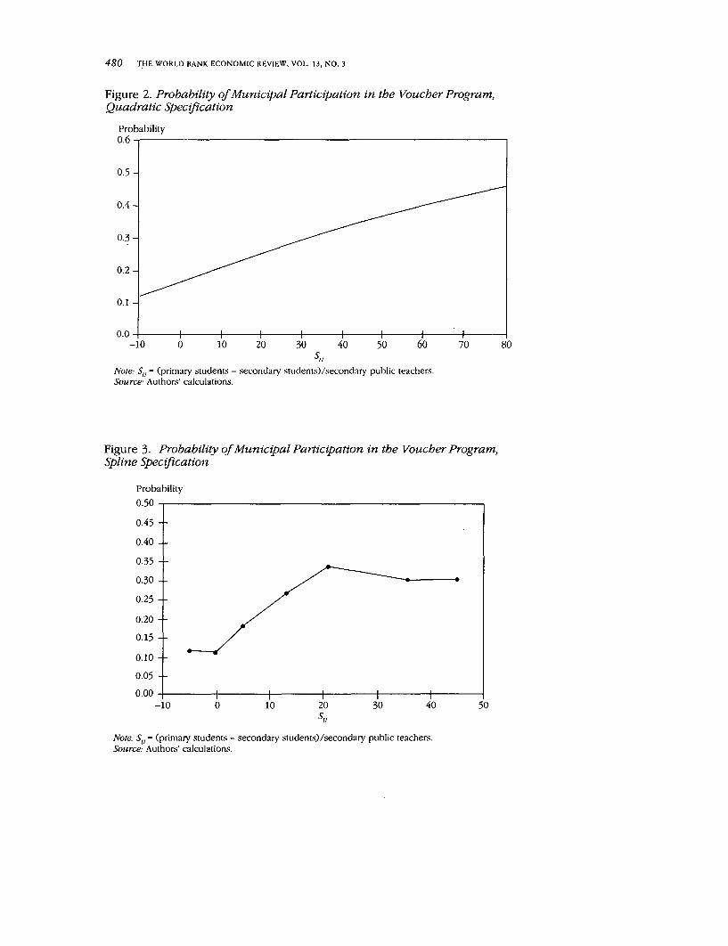
480 THE WORLD BANK ECONOMIC REVIEW, VOL. 13, NO. 3
Figure 2. Probability of Municipal Participation in the Voucher Program,Quadratic Specification
Probability0.6 -
0.5-
0.4-
0.3-
0.2-
0.1
0.0- I l l l I-10 0 10 20 30 40 50 60 70 80
SINote: S,} = (primary studenLs - secondary stuclents)/secondary public teachers.Source Authors' calculations.
Figure 3. Probability ofMunicipal Participation in the Voucher Program,Spline Specification
Probability0.50
0.45
0.40
0.35
0.30
0.25
0.20
0.15
0.10
0.05
0.00--10 0 10 20 30 40 50
St,
Note. Su = (primary students - secondary students)/seconclary public teachers.Source: Authors' calculations.

King, Orazem, and Wohigemuth 481
III. SCHOOL PROGRAM PARTICIPATION
A school could participate in the voucher program only if its municipalityagreed to participate. All private schools were eligible to join. The number ofprivate schools that participated increased steadily between 1992 and 1997.By mid-1995, 1,795 private schools were accepting voucher students. In thissection we examine the school's participation decision both theoretically andempirically.
Model
We assume that private schools compete on both quality, q, and price, f, butthat public schools offer uniform quality, qc at near-zero cost, fG.12 Given theavailable public school, parents will select the ith private school when
(4) U(qi, f,; Z) > U(qG, fG; Z)
where U(.) is parents' indirect utility, and Z are factors that enter utility and areseparable from school quality and price. We assume that school quality raisesutility (Uq > 0), school fees lower utility (U/ < 0), and private school fees exceedpublic school fees (f, > fc). Therefore, parents must believe that the quality ofprivate schools exceeds that of public schools (qi > qG) for the condition in equa-tion 4 to hold.
Since barriers to entry for new private schools appear to be low, we assumethat private schools will earn no economic profits in the long run. Thus f, =AC(qj), the school's average cost of producing quality qi. Consequently, schoolfees must increase with school quality to enable the school to break even."3 Therewill be a level of school quality, qo, and fees, fo, = AC(qo), that will satisfy condi-tion 4 with equality. These levels will define the competitive fringe of privateschools. For competitive schools; fo and qo are dictated by the market, condi-tional on the availability of public schools of quality qG charging fG.
We illustrate the private school market in figure 4. Competitive fringe schoolsmust provide at least quality qo to lure parents away from public schools andmust charge fees of fo to break even (the right panel of figure 4). Schools couldalso offer quality above qo and then compete on both price and quality as in amonopolistically competitive market. In equilibrium such a school offers qualityq, > qo (the left panel of figure 4). Enrollment demand increases as the schoollowers its fees and becomes perfectly elastic as the fees approach fo. However, the
12. This specification contrasts with Manski's (1992) simulation model, which assumes that all privateschools charged the same price and offered the same quality. However, Manski (1992: 360) points outthat his assumption is too restrictive and that "a more realistic model would permit private schools to setdifferent tuition levels, with associated differences in the quality of the schooling that they offer."
13. In Colombia the correlation coefficients between private tuition fees and average mastery levels inmath and language examinations of ninth-grade students are 0.55 and 0.52, respectively. Presumably,there are other school products, such as students' civic awareness or physical safety, that distinguishschools and are not captured by these test scores.

Figure 4. Representative School Demand and Cost Curves for Minimum- and Intermediate-Quality Private Schools
Monopolistically Competitive Schools Competitive Fringe Schools-Monetary unit Monetary unit
X MC(ql)~~~~~~~~~~~C(l
00
AC(qd
m \\X X _ ~~~~~~~ ~ ~~~~~~~~MC(qd,
z fo / D(qG'gG)~~~~~~~f
el en, e,' Enrollment eo Enrollment
ANote f represenLs school fees, and q represents school quality.

King, Orazem, and Wohigemuth 483
school's optimum fee is fl. Because entry is easy, the school cannot earn eco-nomic profits in the long run, so f1 = AC(ql) at an enrollment level of el. Ifall schools decide to offer quality above qo, then all will be monopolisticallycompetitive.
The voucher program may alter school incentives, depending on school qual-ity and fees. Let VM represent the maximum value of the voucher allowed. IfVM < fo, no private school could recoup its marginal cost if it offered the minimumquality.14 If VM = fo, fringe schools would be indifferent between participating andnot participating. Because they can enroll as many students as they want at fothey have no need to acquire additional students through the voucher program.In fact, schools on the minimum-quality fringe have no capacity to absorb addi-tional students. Voucher students would have to displace nonvoucher students toleave the school with enrollment eo and no economic profits.
Even if VM > fo, schools in existence when the program was initiated could notbenefit from the program. Rules prevented schools from raising fees in the firstyear of participation. In subsequent years schools were allowed to raise fees onlyaccording to an officially sanctioned adjustment for inflation. Thus minimum-quality schools could not raise fees above fo, which meant that they could notprofitably raise enrollment beyond eo.
For the monopolistically competitive schools whose quality is higher than q0,the voucher program may provide an incentive to add students. These schoolshave excess capacity because they can lower their average costs by enrolling morestudents. If the voucher is equal to fl, such a school will expand enrollment to el'and earn higher economic profits than it did before the voucher program. Even ifvM < fl, the school could profit from the voucher program by lowering its fees toVM and expanding enrollment according to VM = MC(ql), provided VM is higherthan fm = min AC(ql). If this school participates, it will increase its enrollment toat least em.lS
Monopolistically competitive schools will not participate if VM < fm(q). Be-cause fm increases as quality increases, the highest-quality schools will be thosefor which VM < fi. For these schools the marginal cost of adding a student ex-ceeds the maximum value of the voucher. Of course, high-quality private schoolsthat already offer need-based scholarships might still participate. The voucherprogram would allow these private schools to admit poor students using acofinancing scheme that reduces the burden to their own scholarship program.
14. We assume that schools were not allowed to charge parents more than the amount of the voucher,and, in fact, schools were discouraged from demanding that parents "top up" the voucher. Since voucherswere targeted to the poorest segments of the population, many families did not have much more to offer.
15. In the long run schools will not be able to earn positive economic profits from the vouchers. Newschools will enter. If parents can easily obtain and understand information on school quality, a new set ofvoucher schools will emerge that select quality such that vM = min AC(q) > f0. Therefore, in the long runthe voucher program should increase the number of intermediate-quality schools. However, the poorest-quality schools will exit because they are nlow inferior to voucher schools and are excluded from thevoucher subsidy.

484 THE WORLD BANK ECONOMIC REVIEW, VOL. 13, NO. 3
The simple model illustrated in figure 4 can incorporate cofinancing. Costs ofmany private schools are partially offset by monetary or in-kind assistance fromsponsoring religious or nonsectarian organizations. These transfers lower theschools' average costs by the value of the donation, d, per student. We can alsoadjust the model to incorporate school administrative costs, as. In order to par-ticipate in the voucher program, schools had to attract students, elicit applica-tions from families in the lowest income groups, and cooperate with the regionalprogram agency to verify the continued attendance of each voucher student.
The donations and administrative costs are observed with error, us. The prob-ability that a school offers a positive number of vouchers is
(5) P(V¾ > O) = P{[vm-fm(q,)-aS + d> uJ A [f > fo])
Equation 5 states that the ith private school will participate when the maximumvalue of the voucher plus any per-pupil external support covers the average costof a voucher student, provided that the school is not a minimum-quality privateschool charging fo.
Equation 5 can be operationalized by noting the implied participation incen-tives for a continuum of schools sorted according to fees and quality from lowestto highest. Schools that offer the lowest quality, q0, and charge the lowest feescannot profit from expanding enrollment because rules prevent them from rais-ing their fees in response to the voucher program. Schools that offer intermediatequality and fees can profitably expand enrollment as long as the value of thevoucher exceeds their minimum average costs. Eventually, as we move to schoolswith progressively higher fees and quality, the voucher will fail to cover the mar-ginal cost of an additional student. This suggests a probit equation of the form
(6) p(Vt, >0) = q(fj, fi2 qi, q2, d, a., uJ)+ -+ -+-
where the expected signs are included below the explanatory variables.'" Thetheory suggests a nonlinear relationship between participation and school fees orquality so that schools with intermediate fees and quality will be the most likelyto participate. Because fees and measured quality are not perfectly correlated, weincorporate both in the analysis. Holding the two constant, schools will be morelikely to participate if they have access to external support and if they face lowercosts of administering the voucher program.
Data
The Ministry of Education collected data on schools and students as part of itsSistema Nacional de Evaluaci6n de la Calidad de la Educaci6n (SABER). The Min-istry collected the data in late 1992 or early 1993, the first year in which it was
16. Note that vM is the same for all schools, and so it cannot explain variatioin in thie probabilitv ofparticipation across schools. Its influence is captured in the constant term.

King, Orazem, and Wohlgemuth 485
expanding the voucher system nationally. At that time municipalities could havebeen participating in the program for one year, but most had not yet adopted theprogram. The data on students cover only seventh and ninth graders, none ofwhom qualified to receive the vouchers, since the program was restricted to newsixth graders in 1992-93. Since schools were not allowed to change their fees inthe first year of the program, the data on schools and students predate the influ-ence of the vouchers on school or household attributes.
The sample consists of 71 participating private schools and 77 nonparticipat-ing private schools. The ratio of participation is larger in our sample than in thepopulation of private schools overall because the SABER sampling design is skewedtoward more urban areas.' 7 Consequently, the results should be interpreted asreflecting the decision process of private urban schools.
Monthly fees for schools that participated in the voucher program averagedabout 60 percent of the fees in nonparticipating private schools (table 3). Thenonparticipating schools were also of higher quality, as indicated by higher aver-age scores on the nationwide school-leaving exam given to eleventh-grade stu-dents. Average test scores in the public schools were also higher than those inparticipating private schools, albeit by only a small and insignificant margin.There were other indications that the quality of program schools was lower onaverage than that of nonprogram schools. Participating schools were more likelyto offer nonacademic (vocational or technical) tracks and had higher pupil-teacherratios than did nonparticipating schools. In terms of quality, participating pri-vate schools were more similar to public schools than to nonparticipating privateschools.
Promotional costs of administering the voucher program are likely to differacross schools. Schools that cater to poorer families will have an advantage inidentifying potential voucher recipients. Using counts of household durable goodsto measure household wealth, we find that the wealthiest households tended tobe in nonparticipating schools. Public schools had the lowest average value ofthis indicator.
Estimation and Results
Table 4 reports three sets of probit estimates of the school participation func-tion. Since only schools in participating municipalities could join the voucherprogram, we first investigate whether a school's participation decision was re-lated to the municipality's participation decision. We introduce a correction forpossible selection bias in equation 6, using the inverse Mills ratio derived fromthe estimated municipal participation equation (see table 2). The results, whichwe do not report here, indicate that the probability of municipal participation is
17. Also, the SABER sample includes only schools that educate students through eleventh grade, theterminal year of secondary education. Many schools, primarily in rural areas, educate students only throughninth grade.

486 THE WORLD BANK ECONOMIC REVIEW, VOL. 13, NO. 3
Table 3. Means and Standard Deviations of Variables Used in SchoolParticipation Function
Participating Nonparticipating PublicVariable private schools private schools schools
Monthly fee per student (Colombian pesos) 7,777.1 13,161.5 626.9(4,643.1) (11,140.29) (1,582.8)
Average school-leaving test score 47.6 52.8 49.2(5.1) (7.4) (5.1)
Nonprofit school 0.51 0.53 n.a.(0.50) (0.50) n.a.
Offers academic education 0.75 0.92 0.71(0.44) (0.27) (0.46)
Pupil-teacher ratio 21.9 17.6 20.5(9.7) (8.8) (7.5)
Household assets of students 9.9 10.9 9.1(1.3) (1.6) (1.2)
Sample size 71 77 112
n.a. Not applicable.Note: Standard deviations are in parentheses.Source: Authors' calculations based on program administrative data from ICETEX central and regional
offices, 1995-97, and SABER data, 1992-93.
not correlated with the regressors in the school participation equation.18 Thus wecan interpret the results of the school participation equation as holding for pri-vate schools generally and not just for those in participating municipalities.
The main variables of interest are tuition fees and average test scores. Bothhave the predicted quadratic sign pattern: the probability of participation firstrises and then falls as the variables increase in value. This pattern holds regard-less of whether fees and test scores enter the specification jointly or separately.We take this result as.strong support for the presumption that schools makeparticipation decisions at least partially according to the profit-maximizing modeldescribed above.
The implied impact of fees and test scores on school participation is traced outin figure 5. Participation is highest in the lower half of the range of values forboth fees and test scores. The peak for fees corresponds almost exactly to themaximum value of the voucher and drops off sharply thereafter. Almost no schoolswith fees in the upper half of the tuition range opted to participate. Participationwas more broadly dispersed across school quality as measured by test scores,with many schools in the upper half of the range participating.
These results suggest that the participation decision was tied to a school'sprior fee structure, so that higher-quality schools still participated if they charged
18. The corresponding probit coefficients (and z-statistics) for the inverse Mills ratio for two specificationssimilar to those shown in table 4 are 0.332 (0.92) and 0.218 (0.60). We also employ an alternative procedure,using the variables in table 2 as instruments for the unknown selection process. None of the schoolparticipation coefficients was sensitive to alternative specifications in terms of sign, significance, ormagnitude.
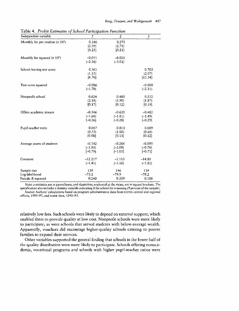
King, Orazeni, and Wohigemuth 487
Table 4. Probit Estimates of School Participation FunctionIndependent variable 1 2 3
Monthly fee per student (x 103) 0.240 0.275(2.39) (2.71)[0.25] [0.21]
Monthly fee squared (x 106) -0.011 -0.021(-2.56) (-3.01)
School-leaving test score 0.561 0.703(1.55) (2.07)[6.76] [11.34]
Test score squared -0.006 -0.008(-1.70) (-2.31)
Nonprofit school 0.624 0.480 0.512(2.18) (1.90) (1.87)[0.17] [0.12] [0.19]
Offers academic stream -0.546 -0.620 -0.482(-1.60) (-1.81) (-1.49)[-0.26] [-0.28] [-0.29]
Pupil-teacher ratio 0.007 0.013 0.009(0.53) (1.00) (0.66)[0.08] [0.13] [0.12]
Average assets of students -0.142 -0.206 -0.095(-1.03) (-2.08) (-0.76)[-0.79] [-1.05] [-0.71]
Constant -12.217 -1.115 -14.81(-1.41) (-1.16) (-1.81)
Sample size 139 146 139Log-likelihood -73.2 -79.9 -78.2Pseudo R-squared 0.240 0.209 0.188
Note: z-statistics are in parentheses, and elasticities, evaluated at the mean, are in square brackets. Thespecification also includes a dummy variable indicating if the school fee is missing (9 percent of the sample).
Source: Authors' calculations based on program administrative data from ICETEX central and regionaloffices, 1995-97, and SABER data, 1992-93.
relatively low fees. Such schools were likely to depend on external support, whichenabled them to provide quality at low cost. Nonprofit schools were more likelyto participate, as were schools that served students with below-average wealth.Apparently, vouchers did encourage higher-quality schools catering to poorerfamilies to expand their services.
Other variables supported the general finding that schools in the lower half ofthe quality distribution were more likely to participate. Schools offering nonaca-demic, vocational programs and schools with higher pupil-teacher ratios were

488 THE WORLD BANK ECONOMIC REVIEW, VOL. 13, NO. 3
Figure 5. Estimated Probability of School Participation over the Range of SchoolFees and Test Scores
Probability
0.7
0.6 Fe
0.5
0.4 Tt scores
0.3
0.2
0.1
00.00 0.10 0.20 0.30 0.40 0.50 0.60 0.70 0.80 0 90 1.00
Index value
Note: The horizontal axis is normnalized to range from 0 to 1 where I corresponds to the highest test scoreor fees in the sample and 0 corresponds to the smallest. lf is the largest fee in the sample and f,,,,, thesmallest, the fee index is defined as (f, ~ j,.Similarly, the test score index is (q, - q~~A, -
q,,,.The probabilities are estimnated with all other variables fixed at their Sample means.Source. Authors' calculations.
more likely to admit vou'cher students. These coefficients were not-precisely esti-mated, however.
The results show that the attributes of participating schools did not reflect theaverage of all private schools. Peak participation occurred in schools at the twen-tieth percentile in the range of fees and at the thirty-fifth percentile in the range oftest scores. Therefore, assuming that private school averages apply to voucherstudents generally overstates the potential gains of the program.
IV. CONCLUSIONS
Colombia's national voucher program demonstrates how a central govern-ment can effectively mobilize local government resources and private providersto alleviate constraints to public provision of education. At the end of five yearsthe program had given vouchers to more than 100,000 secondary school stu-dents throughout the country. However, even with financial incentives from thecentral government, national programs do not necessarily beget universal adop-tion. Only 25 percent of Colombia's municipalities joined the voucher program.Adoption was most likely in municipalities where existing private schools couldexpand capacity, where a large proportion of students were already enrolled inprivate school, and where there was a limited number of underserved students.Municipalities with a very large number of underserved students or whose exist-ing private schools had relatively little capacity opted not to participate in the
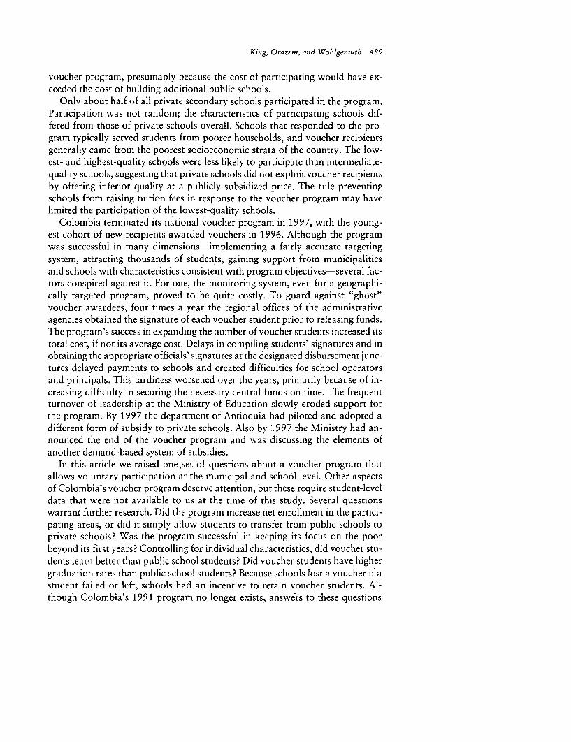
King, Orazem, and Wohigemuth 489
voucher program, presumably because the cost of participating would have ex-ceeded the cost of building additional public schools.
Only about half of all private secondary schools participated in the program.Participation was not random; the characteristics of participating schools dif-fered from those of private schools overall. Schools that responded to the pro-gram typically served students from poorer households, and voucher recipientsgenerally came from the poorest socioeconomic strata of the country. The low-est- and highest-quality schools were less likely to participate than intermediate-quality schools, suggesting that private schools did not exploit voucher recipientsby offering inferior quality at a publicly subsidized price. The rule preventingschools from raising tuition fees in response to the voucher program may havelimited the participation of the lowest-quality schools.
Colombia terminated its national voucher program in 1997, with the young-est cohort of new recipients awarded vouchers in 1996. Although the programwas successful in many dimensions-implementing a fairly accurate targetingsystem, attracting thousands of students, gaining support from municipalitiesand schools with characteristics consistent with program objectives-several fac-tors conspired against it. For one, the monitoring system, even for a geographi-cally targeted program, proved to be quite costly. To guard against "ghost"voucher awardees, four times a year the regional offices of the administrativeagencies obtained the signature of each voucher student prior to releasing funds.The program's success in expanding the number of voucher students increased itstotal cost, if not its average cost. Delays in compiling students' signatures and inobtaining the appropriate officials' signatures at the designated disbursement junc-tures delayed payments to schools and created difficulties for school operatorsand principals. This tardiness worsened over the years, primarily because of in-creasing difficulty in securing the necessary central funds on time. The frequentturnover of leadership at the Ministry of Education slowly eroded support forthe program. By 1997 the department of Antioquia had piloted and adopted adifferent form of subsidy to private schools. Also by 1997 the Ministry had an-nounced the end of the voucher program and was discussing the elements ofanother demand-based system of subsidies.
In this article we raised one set of questions about a voucher program thatallows voluntary participation at the municipal and school level. Other aspectsof Colombia's voucher program deserve attention, but these require student-leveldata that were not available to us at the time of this study. Several questionswarrant further research. Did the program increase net enrollment in the partici-pating areas, or did it simply allow students to transfer from public schools toprivate schools? Was the program successful in keeping its focus on the poorbeyond its first years? Controlling for individual characteristics, did voucher stu-dents learn better than public school students? Did voucher students have highergraduation rates than public school students? Because schools lost a voucher if astudent failed or left, schools had an incentive to retain voucher students. Al-though Colombia's 1991 program no longer exists, answers to these questions

490 THE WORLD BANK ECONOMIC REVIEW, VOL. 13, NO. 3
would provide useful (and rare) evidence about the potential benefits-as well asthe pitfalls-of similar programs in the future.
REFERENCES
The word "processed" describes informally reproduced works that may not be com-monly available through library systems.
Angrist, Joshua, Eric Bettinger, Erik Bloom, Elizabeth M. King, and Michael Kremer.1999. "Vouchers for Private Schooling in Colombia: Evidence from a RandomizedNatural Experiment." Massachusetts Institute of Technology, Harvard University, andthe World Bank. Processed.
CERI, OECD (Centre for Educational Research and Innovation, Organisation for EconomicCo-operation and Development). 1994. School: A Matter of Choice. Paris.
Colombia, Department of National Planning. 1994. "Sistemas de indicadores socio-demograficos para Colombia: Pobreza en el pais y por departamentos." Boletin 5.Bogota. Processed.
Gauri, Varun. 1998. School Choice in Chile: Two Decades of Educational Reform. Pitts-burgh: University of Pittsburgh Press.
Hanson, Mark. 1995. "Democratization and Decentralization in Colombian Education."Comparative Education Review 39(1):101-19.
Henig, Jeffrey R. 1994. Rethinking School Choice: The Limits of the Market Metaphor.Princeton: Princeton University Press.
Hoxby, Caroline M. 1996. "The Effects of Private School Vouchers on Schools and Stu-dents." In H. F. Ladd, ed., Holding Schools Accountable: Performance-Based Reformin Education. Washington, D.C.: Brookings Institution.
James, Estelle. 1993. "Why Do Different Countries Choose a Different Public-PrivateMix of Educational Services?" Journal of Human Resources 28(Summer):571-92.
Jimenez, Emmanuel, Marlaine E. Lockheed, and Vicente Paqueo. 1991. "The RelativeEfficiency of Private and Public Schools in Developing Countries." The World BankResearch Observer 6(July):205-18.
King, Elizabeth M., Laura Rawlings, Marybell Guti6rrez, Carlos Pardo, and Carlos Torres.1997. "Colombia's Targeted Education Voucher Program: Features, Coverage, andParticipation." Impact Evaluation of Educational Reforms Working Paper 3. WorldBank, Washington D.C. Processed.
Lankford, Hamilton, and James Wyckoff. 1992. "Primary and Secondary School Choiceamong Public and Religious Alternatives." Economics of Education Review 11(De-cember):317-37.
Levin, Henry M. 1991. "The Economics of Educational Choice." Economics and Educa-tion Review 10(2):137-58.
. 1992. "Market Approaches to Education: Vouchers and School Choice." Eco-nomics of Education Review 11(4):279-85.
Lockheed, Marlaine, and Emmanuel Jimenez. 1994. "Public and Private Secondary Schoolsin Developing Countries." HRO Working Paper 43. Human Resources and OperationsPolicy Vice Presidency, World Bank, Washington, D.C. Processed.
Manski, Charles F. 1992. "Educational Choice (Vouchers) and Social Mobility." Eco-nomics of Education Review 11(December):3S1-69.

King, Orazem, and Wohlgemith 491
Montenegro, Armando. 1995. "An Incomplete Educational Reform: The Case of Colom-bia." HCO Working Paper 60. Human Capital Development and Operations PolicyVice Presidency, World Bank, Washington, D.C. Processed.
Morales-Cobo, Patricia. 1993. "Demand Subsidies: A Case Study of the PACES VoucherProgram." Department of Economics, University of the Andes, Bogota.
Murnane, Richard J., Stuart Newstead, and Randall J. Olsen. 1985. "Comparing Publicand Private Schools: The Puzzling Role of Selectivity Bias." Journal of Business andEconomic Statistics 3(January):23-35.
Neal, Derek. 1997. "The Effects of Catholic Secondary Schooling on Educational Attain-ment." Journal of Labor Economics 15(January):98-123.
Parry, Taryn Rounds. 1993. "Theory Meets Reality in the Great Voucher Debate." Uni-versity of Georgia. Processed.
Ribero, Rocio M., and Jaime G. Tenjo. 1997. "Evaluaci6n del programa de becas paces."University of the Andes, Bogota. Processed.
Rodriguez, Jorge G. 1988. "School Achievement and Decentralization Policy: The Chil-ean Case." Revista de Andlisis Econ6mico 3(1):1.
Sander, William. 1996. "Catholic Grade Schools and Academic Achievement." Journalof Human Resources 31(Summer):540-48.
Sander, William, and Anthony C. Krautmann. 1995. "Catholic Schools, Dropout Rates,and Educational Attainment." Economic Inquiry 33(April):217-33.
West, Edwin G. 1996. "Education Vouchers in Practice and Principle: A World Survey."Human Capital Development Working Paper 64. World Bank, Washington, D.C.Processed.
Winkler, Donald, and Taryn Rounds. 1996. "Municipal and Private Sector Response toDecentralization and School Choice." Economics of Education Review 15(4):365-76.
Witte, John F. 1996. "School Choice and Student Performance." In Helen F. Ladd, ed.,Holding Schools Accountable: Performance-Based Reform in Education. Washing-ton, D.C.: Brookings Institution.
World Bank. 1994. Poverty in Colombia. Washington, D.C.


THE WORLD BANK ECONOMIC REVIEW, VOL. 13, NO. 3: 493-508
Student Outcomes in Philippine ElementarySchools: An Evaluation of Four Experiments
Jee-Peng Tan, Julia Lane, and Gerard Lassibille
Policymakers in most developinig countries are concerned about high dropout rates andpoor student learning in primary education. The governmenit of the Philippines initiatedthe Dropout Intervention Program in 1990-92 as part of its effort to address theseissues. Under this program, four experimental interventions were randomly assigned to20 schools in selected low-income areas. Pre- and post-intervention data were collectedfrom these schools, as well as from 10 control schools, in order to evaluate the program'simpact on dropout behavior and student learning. The economic justification for repli-cation appears to be strongest for the interventions that provided teachers with learningmaterials, which helped them to pace lessons according to students' differing abilities,and that initiated parent-teacher partnerships, which involved parents in the schoolingof their children. The justification was weakest for the school feeding intervention. Inaddition to the results specific to the Philippines, this research demonstrates the feasibil-ity of monitoring and evaluating interventions in the education sector in other develop-ing countries, including the use of randomized control designs.
Most developing countries now recognize that investing in education, particularlyprimary education, provides an essential bedrock for economic and social develop-ment. In past decades governments emphasized expanding enrollment, but as cov-erage rose, the problems of low completion rates and inadequate student learningcame to the fore (see Lockheed and Verspoor 1991 for a comprehensive treatmentof these issues). Policymakers need information on the costs as well as on the im-pact of different methods of improving schooling outcomes. Unfortunately, how-ever, the literature on the quantitative relationship between inputs and outcomesin education is sparse, and most developing countries have only a nascent capacityto conduct their own context-specific research and evaluation.'
1. See Harbison and Hanusihek (1992) for a summary of results from 96 studies on the relationshipbetween school inputs and learning based on data from developing countries. Quantitative studies on therelationship between school inputs and dropout behavior and between school inputs and grade repetitionare much more rare. Recent examples include Hanushek and Lavy (1994), Gomes-Neto and Hanushek(1994), and Chuard and Mingat (1996).
Jee-Peng Tan is with the Human Development Network at the World Bank, Julia Lane is with the UrbanInstitute, and Gerard Lassibille is with the Centre National de Ia Rccherche Scientifique in Dijon, France. T heauthors' e-mail addresses are [email protected], [email protected], and [email protected] authors thank Ms. Lidi Santos and her staff at the Bureau of Elementary Education of the PhilippinesDepartment of Education, Culture, and Sports for facilitating access to the data, the World Bank's ResearchDepartment for partial financial support, Alain Mingat for helpful discussions on the analytical method, andthree anonymous referees for comments and suggestions on earlier drafts.
©) 1999 The International Bank for Reconstruction and Development/THE WORI.D BANK
493

494 THE WORLD BANK ECONOMIC REVIEW, VOL. 13, NO. 3
This article documents an evaluation effort in the Philippines intended to guidepolicymaking in primary education. Almost all children in the country enter firstgrade, but not all of them reach the end of the primary school cycle. Data for theearly 1990s suggest that noncompleters represent about 25 percent of each enter-ing cohort of first graders. Further, many children leave school having learnedonly a fraction of the primary school curriculum (Miguel 1993). Achievementtests administered in the 1991 Household and School Matching Survey, for ex-ample, show that pupils in grades two to six mastered less than half of the cur-riculum they were taught (Tan, Lane, and Coustere 1997).
As part of its strategy to improve primary education, the Philippine govern-ment implemented the Dropout Intervention Program (DIP) in the context of aWorld Bank-financed elementary education project. The program comprised fourexperimental interventions. Each of these was implemented in five schools dur-ing the 1991-92 academic year, for a total of 20 schools. As its name suggests,the DIP focused primarily on reducing dropout rates, but it was also expected toimprove student learning.
To determine whether or not the pilot interventions should be replicated, thegovernment randomly assigned them to schools in select low-income communi-ties and collected both pre- and post-intervention data over two school years.The government also collected data on schools that were not part of the programto provide a benchmark for assessing the impact of the interventions. The result-ing data set is rare in a developing country.2 Thus while one goal of this paper isto shed light on elementary education policy in the Philippines, a broader aim isto demonstrate that project evaluation in developing countries is both feasibleand worthwhile.
I. THE DIP INTERVENTIONS
The DIP consisted of four experimental interventions: school feeding; multi-level learning materials, which are pedagogical materials for teachers; school feed-ing combined with parent-teacher partnerships; and multi-level learning materi-als combined with parent-teacher partnerships.3 On a per-student basis schoolfeeding is very expensive, the use of multi-level learning materials is considerablycheaper, and parent-teacher partnerships entail minimal additional costs becausethey involve mostly an adjustment in the way parents interact with teachers. Thesubstantial differences in costs of the three interventions make it especially im-portant to compare them in terms of both benefits and costs.
2. For recent examples of the evaluation of social sector programs based on randomized control designs,see Newman, Rawlings, and Gertler (1994). See Glewwe, Kremer, and Moulin (1997) for a recent applicationto education.
3. Parent-teacher partnerships envision a more active role for parents than they are commonly assigned,especially in developing countries. See Epstein (1991) for a discussion of how teachers' interactions withparents can improve student achievement.

Tan, Lane, and Lassibille 495
Under the school feeding intervention all pupils in beneficiary schools receiveda free school meal while classes were in session. Because of substitution effects,this intervention may not increase pupils' food intake, as Jacoby (1997a, 1997b),for example, suggests. This problem is inherent to all feeding programs. Since wehave no way to quantify the amount of substitution between food provided athome and food provided under the DIP, any change associated with the interven-tion must necessarily be interpreted as its net rather than its gross impact.
Under the multi-level learning materials intervention, all teachers in the ben-eficiary schools received pedagogical materials designed to help them pace theirteaching according to the differing abilities of their students. Prior to implemen-tation of the DIP, teachers attended a week-long training course on the use of thematerials. Parent-teacher partnerships comprised a series of regular (usuallymonthly) group meetings throughout the school year between school staff andparents. The authorities chose to implement parent-teacher partnerships in com-bination with one of the other two interventions (rather than on its own) becausethe other interventions provided a way to attract parents to the meetings andprovided the substantive focus for meetings.
The DIP project team, which was part of the Bureau of Elementary Education,followed a three-stage procedure in selecting schools for the interventions. Theyfirst identified five regions of the country and, within each region, two districtsthat met the official definition of a low-income municipality (the municipalityhad to meet at least three of five poverty criteria relating to education, health,housing, unemployment, and household consumption). The sample schools werelocated in 10 provinces: Mindoro Oriental and Palawan in Southern Luzon Re-gion, Camarines Sur and Sorsogon in Bicol Region, Ilioilo and Negros Occiden-tal in Western Visayas Region, Northern Samar and Western Samar in EasternVisayas Region, and North Cotabato and Maguindanao in Central MindanaoRegion. In one district the treatment choices were packaged as no intervention,multi-level learning materials, or multi-level learning materials combined withparent-teacher partnerships, while in the other district they were packaged as nointervention, school feeding, or school feeding combined with parent-teacherpartnerships. The decision of which of the two intervention packages to assign toeach site in the region was made by the toss of a coin.
Next, in each district the project team selected three schools that met the fol-lowing criteria: each school offered all grades of instruction in the elementarycycle, with one class of pupils per grade; had a high dropout rate, based on ad-ministrative records; was not located in an area with security risks; and did notoffer any school feeding services. Each school was typically the only school in itslocality. Finally, by random drawing, the three schools in each district were as-signed to the control group or to one of the two intervention options. The pro-cess generated a sample of 20 intervention schools and 10 control schools. Oneschool from the control group was eventually dropped because of logistical diffi-culties in collecting data.
496 TfiE WORLI) BANK ECONOMIC REVIEW, VOL. 13, NO. 3
The use of random assignment yields evaluation results that are both convinc-ing to researchers and easy for policymakers to understand (Burtless 1995).Heckman and Smith (1995) point out that selection bias may remain a problemin randomized trials because people in treatment groups may opt out of the treat-ment and those in the control group may compensate for their exclusion from theexperiment. In the DIP evaluation, schools in the treatment group could not selectinto or out of the assigned interventions, and schools in the control group couldnot substitute other types of educational interventions to compensate for notbeing in the treatment group. However, because resources were scarce, the projectteam found it necessary to strike a balance between the priority of addressingpressing needs in poor schools and the advantage for program-evaluation of hav-ing complete randomization in the placement of interventions. In the end theprogram team decided to target the interventions to needy districts and schools.Although randomized selection was not used to identify the two districts in eachregion nor the schools in each district, it was the basis for assigning the twointervention packages to the sites in each region and for assigning treatment orcontrol status to schools.
II. DATA COLLECTION
The interventions were implemented in the 1991-92 school year, but datacollection began in 1990-91 to generate baseline information (table 1). Datawere collected from all pupils in all grades in each sample school. Because theschools had only one section per grade, being poor rural schools, the resultingdata set has information on the full population of students.4
The data include the characteristics of the schools and the classroom environ-ment (including teacher characteristics), as well as information about the pupils:family and personal background; scores on grade-specific tests in mathematics,English, and Filipino, with one set of tests administered at the start of the schoolyear and a second set administered at the end; and transition to the next schoolyear. The survey also attempted to record students' daily attendance throughoutthe school year, but the data proved unreliable because of poor record-keeping.The data on transition to the next grade comprised two kinds of information: theschool management's year-end decision to promote the pupil to the next grade orretain him or her in the same grade, and whether or not the pupil actually re-turned the next school year.
The data are two-year records of pupils' transition through school for thosewho remained in the sample for both years of the study-that is, those whoentered first through fifth grade in year one and who did not drop out. (Therewere very few transfers to other schools because most of the schools in the projectsites were the only ones in their locality). The transition record is truncated for
4. We account for this feature of the sampling procedure in the multivariate regression analyses belowby allowing for a school- or teacher-level structure in the variance-covariance error term.

Tan, Lane, and Lassibille 497
Table 1. Sample Composition in the Philippine Dropout InterventionProgram, 1990-92
Number of Number of pupils'Intervention schools 1990-91 1991-92
Full sample 29 4,267 3,953
Program interventionNo intervention 9 1,356 1,279School feeding
Alone 5 751 695
With parent-teacher partnership 5 858 792Multi-level learning materials
Alone 5 673 634With parent-teacher partnership 5 629 553
a. Includes only pupils in grades one to five with data on personal and family background who advancedto the next school year.
Source: Survey data from the 1990-92 Dropout Intervention Program.
sixth graders in year one and first graders in year two. Sixth graders had leftprimary school by the second year, and their schooling career was not tracked; asa result, their data are for year one only. First graders in year two have no datafor year one, since they were not yet in primary school.
As with any complicated effort to collect data that involves many actors, thedata that eventually became available had some shortcomings. Unlike the drop-out and transition data, the data on student performance were collected for oneyear only. The original intention was to gather longitudinal data, but unforeseencoding problems prevented that. 5 Thus only the achievement data for year one-comprising scores at the start and at the end of the year-could be linked to thedata on student background. Fortuitously, in year two the same achievementtests were administered to the new cohort of entering first graders. Adding thesepupils to the first graders from year one produced a data set containing the infor-mation needed to evaluate the impact of the interventions on student learningamong first graders. Since schooling outcomes in first grade turn out to be espe-cially relevant to elementary education policy in the Philippines-that is, the drop-out problem is concentrated in the first grade-the lack of suitable data for theother grades proved to be a less serious flaw than appeared at first sight.
To confirm that the DIP interventions were in fact randomly assigned acrossschools, we compared dropout rates and student learning as well as students'socioeconomic background in treatment schools and control schools prior to theimplementation of DIP. The results suggest that in terms of the outcome vari-ables-dropout rates and year-end test scores-the treatment schools are notsignificantly different from the control schools (table 2). The random assignment
5. The identification codes on the achievement files from the second year lacked sufficient detail topermit secure matches to the data from the first year. The files on attendance and transition status werecollected using a separate procedure and did not suffer from this flaw.

498 THE WORLD BANK ECONOMIC REVIEW, VOL. 13, NO. 3
Table 2. Pupils in Control and Treatment Schools Prior to Implementing theDropout Intervention Program
Schools thatSchools that received the multi-levelreceived the learning materials
school feeding intervention interventionWith parent- With parent-
Control teacher teacherVariable schools Alone partnership Alone partnership
Outcome variablesMean dropout rate
(percent) 9.56 8.58 7.02** 9.29 10.01Mean z-score on year-
end testa 0.02 0.01 0.07 -0.10 -0.10
Student characteristicsPercent repeating current
grade 0.21 0.28* 0.23 0.24 0.27Percent attended preschool 19.8 14.6* 10.6** 21.1 13.5**Percent whose father is
a farmer 47.2 53.6* 47.9 36.2** 44.9Percent from non-Tagalog-
speaking homes 48.9 52.4* 57.1** 33.1** 32.0**Mean years of mother's
schooling 6.0 5.8* 5.5** 6.3** 6.1Mean number of brothers
and sisters 5.2 5.1 4.7** 5.4 4.7*Mean z-score on entering
test' 0.06 -0.14* 0.19** 0.15 -0.41*
Deviation from the control group is statistically significant at the 5 percent level.** Deviation from the control group is statistically significant at the 1 percent level.a. Test scores are for first graders only. They are expressed in units of standard deviation from the
sample mean.Source: Authors' calculations.
process thus appears to have been valid, implying that a simple analysis of thedifferences between the mean impacts on the control and treatment groups wouldcapture average treatment effects.
The schools are less similar, however, with regard to pupil characteristics. Inparticular, children in schools that received the school feeding program appear tobe systematically less well off than children in the control schools. The presenceof such differences is not surprising, given the relatively small number of schoolsin the sample. Below we use multivariate methods to control for these differencesin evaluating the impact of the DIP interventions.
III. THE IMPACT OF THE DIP INTERVENTIONS
Dropout rates decline in all sample schools between the pre- and post-treat-merit years (table 3). However, the decline is statistically significant only in theschools that received multi-level learning materials, with or without parent-teacher
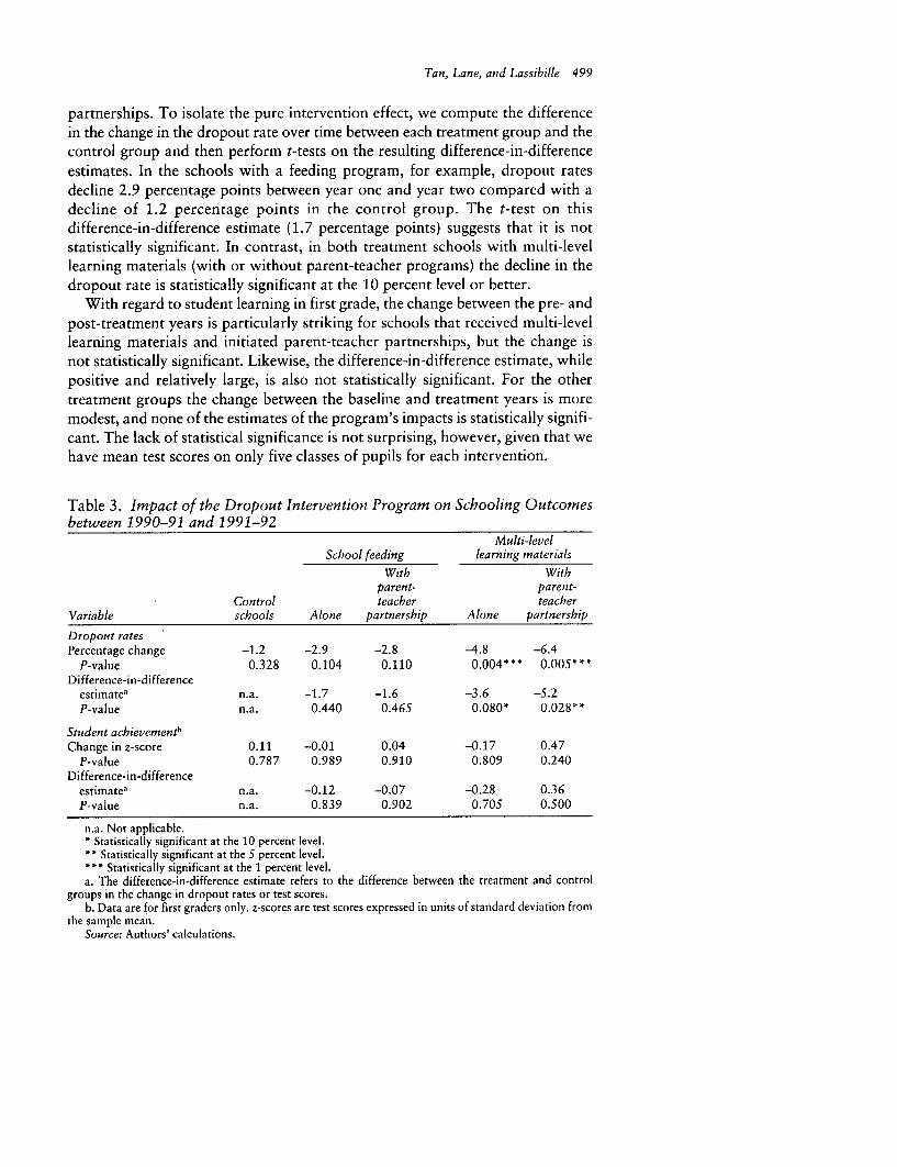
Tan, Lane, and Lassibille 499
partnerships. To isolate the pure intervention effect, we compute the differencein the change in the dropout rate over time between each treatment group and thecontrol group and then perform t-tests on the resulting difference-in-differenceestimates. In the schools with a feeding program, for example, dropout ratesdecline 2.9 percentage points between year one and year two compared with adecline of 1.2 percentage points in the control group. The t-test on thisdifference-in-difference estimate (1.7 percentage points) suggests that it is notstatistically significant. In contrast, in both treatment schools with multi-levellearning materials (with or without parent-teacher programs) the decline in thedropout rate is statistically significant at the 10 percent level or better.
With regard to student learning in first grade, the change between the pre- andpost-treatment years is particularly striking for schools that received multi-levellearning materials and initiated parent-teacher partnerships, but the change isnot statistically significant. Likewise, the difference-in-difference estimate, whilepositive and relatively large, is also not statistically significant. For the othertreatment groups the change between the baseline and treatment years is moremodest, and none of the estimates of the program's impacts is statistically signifi-cant. The lack of statistical significance is not surprising, however, given that wehave mean test scores on only five classes of pupils for each intervention.
Table 3. Impact of the Dropout Intervention Program on Schooling Outcomesbetween 1990-91 and 1991-92
Multi-levelSchool feeding learning materials
With Withparent- parent-
Control teacher teacherVariable schools Alone partnership Alone partnership
Dropout ratesPercentage change -1.2 -2.9 -2.8 -4.8 -6.4
P-value 0.328 0.104 0.110 0.004*** 0.005***Difference-in-difference
estimate' n.a. -1.7 -1.6 -3.6 -5.2P-value n.a. 0.440 0.465 0.080* 0.028**
Student achievementbChange in z-score 0.11 -0.01 0.04 -0.17 0.47
P-value 0.787 0.989 0.910 0.809 0.240Difference-in-difference
estimate3 n.a. -0.12 -0.07 -0.28 0.36P-value n.a. 0.839 0.902 0.705 0.500
n.a. Not applicable.* Statistically significant at the 10 percent level.* * Statistically significant at the 5 percent level.
* Statistically significant at the 1 percent level.a. The difference-in-difference estimate refers to the difference between the treatment and control
groups in the change in dropout rates or test scores.b. Data are for first graders only. z-scores are test scores expressed in units of standard deviation from
the sample mean.Source: Authors' calculations.

500 THE WORLD BANK ECONOMIC REVIEW, VOL. 13, NO. 3
These results suggest that the impact of the DIP interventions is ambiguous,positively affecting dropout behavior, but not influencing student learning. Giventhe systematic differences in student characteristics between the treatment andcontrol groups, as well as the small samples involved, such a pattern is expected.Including more test sites for each of the DIP interventions would have broughtmore clarity, but it also would have required many more resources than the gov-ernment was willing or able to allocate to the exercise. Indeed, in most develop-ing countries large-scale experiments are rarely affordable as routine proceduresfor policy analysis. We can nonetheless exploit the data generated from the DIP'S
experimental design by conducting a multivariate analysis to control for the sys-tematic differences between the control and intervention groups. For this analy-sis we use pupils rather than schools as the unit of observation.
Multivariate Analysis
As above, we focus on dropout behavior and student learning as the relevantoutcomes for evaluating the DIP interventions. Following the literature (for ex-ample, Hanushek and Lavy 1994), we postulate that the probability that child idrops out of school s at time t (DP,,,) depends on the child's personal character-istics (PC,) and family background (FB,), the learning environment (LE,,), andthe characteristics of the community (CCi).in which he or she lives. Each DIP
intervention j (INTER,) can affect both dropout behavior and student learning.The school feeding intervention, for example, lowers the cost of schooling, thusboosting the incentives for parents to keep children in school. At the same time,it can improve children's geiieral health and attentiveness, thereby stimulatingacademic progress and lowering the chances of dropping out. The provision ofmulti-level learning materials aims to improve the effectiveness of the pedagogi-cal process. Thus it could potentially heighten children's interest in school as wellas enhance their learning. Both would reduce the probability of dropping out.Finally, parent-teacher partnerships expand parents' involvement in the school-ing of their children, thereby minimizing the influence of adverse social and aca-demic factors on dropout behavior.
More formally,
(1) DP,,, = P + jlPCi + f 2FB, + P3LE,, + P4CCi + ,B5INTER,, + S
In measuring the impact of the DIP on student learning, we again follow theliterature (for example, Harbison and Hanushek 1992) in postulating that childi's academic performance in school s at time t, AP,,,, is a function of his or herinitial achievement, APis, 1, personal characteristics (PCj), and family background(FB,), as well as the learning environment (LE,,), and community characteristics(CC,):
(2) AP,, = o+ 8,APiS, 1, + 32PC,+ 63FB,+8 64LE,, + 85CC, + 56 INTER,, + £
Two important econometric issues-discussed fully in Angrist and Krueger(1999) and Vella (1998)-arise in the estimation of equation 2. The first is the

Tan, Lane, and Lassibille 501
presence of a lagged dependent variable, which, while providing an importantcontrol factor, may be correlated with the error term. This problem can be ad-dressed by choosing instrumental variables that are correlated with the laggedvariable but not with the error term. We choose the lagged values of scores onother tests as instruments. Of course, the reduction in bias comes at the expenseof a loss of efficiency, and the reliability of this approach depends on the validityof the instruments. In our case the r-squared values of the correlation betweenthe instruments and the lagged values range from 0.43 to 0.50, suggesting someloss of efficiency and a consequent downward bias in the t-statistics.
The second econometric issue is that of selection bias associated with drop-ping out. Since the weakest students are those who are most likely to drop out,the analysis of student learning is performed on a censored sample. Although thedominant method of correcting for this problem is to apply a Heckman two-stepcorrection by constructing an index based on the probability of censoring, thereis some dissatisfaction with this approach, as Hamermesh (1999) describes.6 Theindex is based on the assumption of a normal distribution, and, as Hamermeshnotes, the results are extremely sensitive to distributional assumptions. Furtherconcerns are often raised about the choice and adequacy of identifying variablesin the first step, although in our case we are fortunate in having detailed informa-tion on variables in equation 1 that affect the cost of education but are not di-rectly associated with a child's academic performance. In particular, we havedata on the distance to school, whether or not the father is a farmer (since animportant opportunity cost of schooling in poor rural communities is children'scontribution to farm work), and whether or not the student is the oldest child inthe family.
A number of alternative approaches have been proposed to deal with selectionbias-nonparametric and semiparametric methods, as well as nonindex-orientedmodels-although no consensus has yet emerged as to which is preferred. Conse-quently, we estimate and report the results from three separate procedures.' As abasis for comparison, we first report the results of a simple regression of year-endtest scores against the intervention variables and control factors, with no correc-tion for selection bias. Then we use a nonindex instrumental variable approach,following Krueger (1997), in which we simply assign to students who have droppedout their academic ranking based on their initial test score. Finally, we follow theconventional Heckman approach, which includes the Mills ratio as an additionalregressor in equation 2. It should be noted that in the Heckman approach thestandard errors are biased because it is impossible to estimate them correctlywhen simultaneously applying that procedure and using instrumental variablesto correct for the problem of lagged dependent variables.
6. Noteworthy, however, is Vella's (1998) finding that the Heckman approach performs quite wellcompared with other approaches.
7. In all three approaches we correct for the problem of having a lagged dependent variable by usingthe instrumental variables procedure described above.
502 THE WORLD BANK ECONOMIC REVIEW, VOL. 13, NO. 3
To estimate equation 1 we use data for pupils from the first to fifth grades inorder to increase the sample size for analyzing what in statistical terms is still arelatively rare event. We could not include pupils from the sixth grade becausetheir dropout record is incomplete for reasons explained earlier. We represent apupil's characteristics and family background as a vector of commonly used vari-ables, such as the child's sex and mother's education. 8
Regression Results
The full dropout regression model, with controls for the complete range of back-ground factors, achieves a reasonable overall goodness-of-fit, with a Hosmer-Lemeshow chi-squared statistic of 13.28 (column 2 of table 4). We also estimate asimplified model using only the interventions as regressors in order to see whetherthe interventions were correlated with the background variables (column 3 of table4).9 Not surprisingly, the simplified regression model as a whole has no explana-tory power; it is nonetheless noteworthy that all of the coefficient estimates arecomparable to the corresponding estimates in the full model. Moreover, in bothregressions only the intervention involving the use of multi-level learning materialshas a measurable effect on dropout behavior. The positive impact of this interven-tion is consistent with the results based on sample means (see table 3). Those re-sults also suggest that interventions combining the use of multi-level learning mate-rials with parent-teacher partnerships have a positive impact.
We then estimate equation 2 for the three different subjects-mathematics,Filipino, and English. Students were given tests in these subjects at both the startand end of the school year (table 4).10 The first feature of the results is that nointervention consistently improves student learning across all three subjects, afinding that jibes with the data in table 3, which are based on average perfor-mance across the three subjects. For both Filipino and English the coefficients onthe intervention involving multi-level learning materials combined with parent-teacher partnerships are statistically significant in all three regressions. The coef-ficients are comparable in magnitude, especially in the regressions for English.
For English the coefficients on the school feeding intervention, whether aloneor combined with the parent-teacher partnerships, are statistically significant onlyin the two regressions that control for selection bias (the second and third col-umns in each subject block). For mathematics the coefficient on school feedingcombined with parent-teacher partnerships is also statistically significant in bothregressions adjusted for selection bias. Overall, the findings suggest that the DIP
interventions are better at helping students learn languages than mathematics.Further, the interventions involving the use of multi-level learning materials, as
8. Father's education is almost perfectly collinear with mother's; we use the latter because the motheris more likely to provide help with homework.
9. We thank an anonymous referee for suggesting this specification.10. In addition to the variables mentioned above, we also include teacher and school fixed effects. For
each subject we use incoming test scores on the other two subjects to instrument the incoming test score.

Tan, Lane, and Lassibille 503
currently designed and implemented, appear to produce more consistent resultsthan do the other components.
IV. POLICY IMPLICATIONS
To assess the policy implications of the DIP, we need to consider both its costand impact. We can assess these qualitatively with available cost data and ourinterpretation of the regression results discussed above (table 5). The underlyingcost data are drawn from implementation records kept by the Bureau of Elemen-tary Education. The school feeding program costs an average of P946 (pesos)per beneficiary, with a range between P621 and P1,054. The multi-level learningmaterials program involved only pedagogical materials, which cost an average ofP90 per child, and the parent-teacher partnerships involved monthly meetingsthat cost an average of about P33 per child (in direct costs). To be perfectlycomparable, these costs should be adjusted for the opportunity cost of time-that of teachers supervising the school feeding program, that of parents and teach-ers in parent-teacher partnerships, and that of people who train teachers to usethe multi-level learning materials. The cost of the multi-level learning materialsprogram should also be adjusted to reflect the fact that the pedagogical resourcesit provides have a typical lifetime of more than one year. Without making theadjustments explicit, however, the existing cost data already point to an obviousranking of the interventions, with school feeding at the high end, followed bymulti-level learning materials and parent-teacher partnerships at the low end.
The impact of the interventions on dropout behavior and student learningrange from nonexistent (0) to promising (++++). The ranking reflects our inter-pretation of the results from the difference-in-difference estimates and the regres-sion analysis. If none of the analyses shows an appreciable impact, we categorizethe intervention as having zero impact; if the results are consistently positiveacross all or most of the estimation methods and the magnitude of the impact isrelatively large, we label the intervention promising and assign it three or fourpluses to reflect the degree of consistency; and if the results are sporadically posi-tive, we categorize the intervention as having a weak impact, assigning it onlyone or two plus signs.
Given these cost and benefit criteria, the combination of multi-level learn-ing materials and parent-teacher partnerships appears to be the most cost-effective. In contrast, the school feeding intervention, at least in the form imple-mented in DIP, seems to be a weak candidate for replication. This does notimply that a more targeted program-directed, for example, at only the mostmalnourished and underprivileged children-would not be cost-effective. Thatpossibility cannot be confirmed, however, with the data available here. Note,though, that the impact on student learning of multi-level learning materials incombination with parent-teacher partnerships is probably limited to instruc-tion in languages.

Table 4. Regression Results of the Impact of the Dropout Intervention ProgramYear-end test scores (first graders only)
Math Filipino EnglishCorrection for Correction for Correction forselection bias selection bias selection bias
Probability No Using No Using No Usingof dropping correction nonindex correction nonindex correction nonindexout (first to for instrumental Using for instrumental Using for instrumental Using
fifth graders) selection variable Heckman's selection variable Heckman's selection variable Heckman'sIndependent variable (1) (2) bias approach approach bias approach approach bias approach approachIntervention variables.School feeding -0.254 -0.255 0.241 0.248 0.121 0.317 0.160 0.031 0.317 0.323 0.009
(0.56) (1.26) (0.77) (2.72)** (1.36) (1.80) (1.82) (0.32) (1.80) (3.63)** (3.73)**Multi-level materials -0.428 -0.458 -0.092 -0.045 -0.008 0.647 0.234 0.178 0.647 0.548 0.543
(1.71) * (1.99)* (0.18) (0.38) (0.07) (1.66) (2.05)* (1.42) (1.66) (4.71)** (0.66)School feeding with
parent-teacherpartnerships -0.311 -0.319 0.370 0.347 0.277 0.458 0.114 0.058 0.458 0.442 0.544
(1.40) (1.63) (0.84) (3.74)** (3.08)** (1.63) (1.28) (3.31) " (1.63) (4.89)** (1.66)*Multi-level materials
with parent-teacherpartnerships -0.410 -0.367 0.217 0.210 0.081 0.870 0.225 0.309 0.870 0.754 1.048
(1.15) (1.56) (1.50) (1.83) (0.76) (3.12)** (2.02)* (2.65)** (3.12)** (6.64)** (8.83)**Initial test scores
(instrumented)b 0.510 0.607 0.520 0.373 0.618 0.473 0.373 0.485 0.341(8.69)** (18.07)** (1S.16)** (5.11)** (18.51)** (13.98)** (5.11)** (13.83)** (9.99)**
Pupil is a girl -0.172 0.153 0.116 0.171 0.290 0.224 0.246 0.290 0.240 0.181(1.61) (2.64)* (2.95)** (4.43)** (4.57)* * (5.89)** (4.46)*t (4.57)** (6.24)** (2.08)*
Attended preschool -0.211 -0.151 -0.173 -0.096 -0.014 -0.045 0.468 -0.014 -0.039 0.500(1.08) (2.12)* (2.96)** (1.61) (0.25) (0.79) (3.57)** (0.25) (0.69) (1.18)
Mother's years ofeducation -0.072 0.013 0.016 0.007 0.001 0.010 0.004 0.001 0.000 -0.006
(3.22)** (1.16) (2.11)* (0.87) (0.15) (1.32) (0.44) (0.15) (0.03) (2.22)*Father is a farmer -0.070 0.026 0.024 -0.035 -0.103 -0.002 0.143 -0.103 -0.122 -0.081
(0.52) (0.26) (0.47) (0.74) (0.86) (0.04) (1.28) (0.86) (2.44)* (1.52)Non-Tagalog speaker -0.140 -0.031 0.000 0.028 -0.005 0.183 0.014 -0.005 0.009 0.034
(0.86) (0.26) (0.01) (1.04) (0.03) (3.33)** (2.85)** (0.03) (0.16) (0.54)

Eldest child 0.092(0.70)
Repeated previous grade 0.327(2.68)**
Child has activepersonalityc -0.133
(0.62)Family income
(pesos per year) -0.109(1.24)
Distance to school(kilometers) 0.450
(0.88)Distance squared -0.125
(0.97)Hosmer-Lemeshow x2 13.28 0.00
(p-value) (10.25) (1.00)Inverse Mills ratio -0.087 -0.351 -0.471
(standard errors) (0,178) (0.122) (0.099)Number of observations 8,229 8,229 1,676 1,676 1,676 1,676 1,676 1,676 1,676 1,676 1,676R-squared 0.41 0.41 0.43 0.45 0.42 0.44
* Statistically significant at the 10 percent level.* * Statistically significant at the 5 percent level.
* Statistically significant at the 1 percent level.Note: The t-statistics (in parentheses) are consistent with standard errors adjusted for group-specific heteroskedasticity using the Huber-White correction procedure. For
the dropout regression the standard errors are adjusted for clustering on schools. For the test score regressions the standard errors are adjusted for clustering on teachers. Thedropout regressions include dummy variables for grades.
a. The intervention variables are defined as dummy variables that take on the value of 1 when the school attended by the child is a recipient of the indicated interventionand zero otherwise.
b. Tests scores at start of the school year, instrumented by scores on the other two subjects.c. As assessed by pupil's teachers.Source: Authors' calculations.
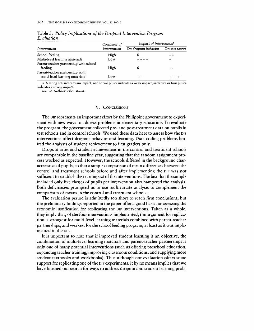
506 THE WORLD BANK ECONOMIC REVIEW, VOL. 13, NO. 3
Table 5. Policy Implications of the Dropout Intervention ProgramEvaluation
Costliness of Impact of interventionaIntervention intervention On dropout behavior On test scores
School feeding High 0 + +Multi-level learning materials Low +.+ + + +Parent-teacher partnership with school
feeding High 0 + +Parent-teacher partnership with
multi-level learning materials Low + + . . . .
a. A rating of 0 indicates no impact, one or two pluses indicates a weak impact, and three or four plusesindicates a strong impact.
Source: Authors' calculations.
V. CONCLUSIONS
The DIP represents an important effort by the Philippine government to experi-ment with new ways to address problems in elementary education. To evaluatethe program, the government collected pre- and post-treatment data on pupils intest schools and in control schools. We used these data here to assess how the DIP
interventions affect dropout behavior and learning. Data coding problems lim-ited the analysis of student achievement to first graders only.
Dropout rates and student achievement in the control and treatment schoolsare comparable in the baseline year, suggesting that the random assignment pro-cess worked as expected. However, the schools differed in the background char-acteristics of pupils, so that a simple comparison of mean differences between thecontrol and treatment schools before and after implementing the DIP was notsufficient to establish the true impact of the interventions. The fact that the sampleincluded only five classes of pupils per intervention also hampered the analysis.Both deficiencies prompted us to use multivariate analysis to complement thecomparison of means in the control and treatment schools.
The evaluation period is admittedly too short to reach firm conclusions, butthe preliminary findings reported in the paper offer a good basis for assessing theeconomic justification for replicating the DIP interventions. Taken as a whole,they imply that, of the four interventions implemented, the argument for replica-tion is strongest for multi-level learning materials combined with parent-teacherpartnerships, and weakest for the school feeding program, at least as it was imple-mented in the DIP.
It is important to note that if improved student learning is an objective, thecombination of multi-level learning materials and parent-teacher partnerships isonly one of many potential interventions (such as offering preschool education,expanding teacher training, improving classroom conditions, and supplying morestudent textbooks and workbooks). Thus although our evaluation offers somesupport for replicating one of the DIP experiments, it by no means implies that wehave finished our search for ways to address dropout and student learning prob-

Tan, Lane, and Lassibille 507
lems in the Philippines. Further, given that the experiment was effective mainly inpromoting student performance in Filipino and English, other measures clearlyneed to be considered if improved performance in mathematics is also desired.
The search for cost-effective strategies to improve schooling outcomes is anissue in all countries. Often, however, such work is hampered by the absence of aroutine system for assessing alternative investment options. The fact that the DIP
was implemented and evaluated augurs well for the future, the problems encoun-tered notwithstanding. It shows that the institutional capacity to evaluate socialexperiments properly exists or can be nurtured within ministries of education orrelated agencies. The task of building research capacity, particularly when theinstitutions involved are outside of academia, is undeniably difficult. The ben-efits are probably worth the effort, however, because the scope for mistakes inthe choice of investment decisions is wide in the absence of quantitative informa-tion about education processes. And these mistakes are costly, not only in finan-cial terms, but also in terms of hindering children's education.
REFERENCES
The word "processed" describes informally reproduced works that may not be com-monly available through library systems.
Angrist, Joshua, and Alan Krueger. 1999. "Empirical Strategies in Labor Economics." InOrley Ashenfelter and David Card, eds., Handbook of Labor Economics. Amsterdam:North-Holland Press.
Burtless, Gary. 1995. "The Case for Randomized Field Trials in Economic and PolicyResearch." Journal of Economic Perspectives 9(2):63-84.
Chuard, Dominique, and Alain Mingat. 1996. "Analysis of Dropout and Student Learn-ing in Primary Education in South Asia." Asian Development Bank, Manila. Processed.
Epstein, Joyce L. 1991. "Effects on Student Achievement of Teacher Practices of ParentInvolvement." In Steven Silvern, ed., Advances in Reading/Language Research. Vol. 5:Literacy through Family, Community, and School Interaction. Greenwich, Conn.: JAIPress.
Glewwe, Paul, Michael Kremer, and Sylvie Moulin. 1997. "Textbooks and Test Scores:Evidence from a Prospective Evaluation in Kenya." Development Economics ResearchGroup, World Bank, Washington, D.C. Processed.
Gomes-Neto, Joao Batista, and Eric A. Hanushek. 1994. "The Causes and Consequencesof Grade Repetition: Evidence from Brazil." Economic Development and CulturalChange 43(1):117-48.
Hamermesh, 'Daniel S. 1999. "The Art of Labormetrics." In Orley Ashenfelter and DavidCard, eds., Handbook of Labor Economics. Amsterdam: North-Holland Press.
Hanushek, Eric A., and Victor Lavy. 1994. "Schooling Quality, Achievement Bias, andDropout Behavior in Egypt." Living Standards Measurement Study Working Paper 107.Development Economics Research Group, World Bank, Washington, D.C. Processed.
Harbison, Ralph W., and Eric A. Hanushek. 1992. Educational Performance of the Poor:Lessons from Rural Northeast Brazil. New York: Oxford University Press.
Heckman, James J., and Jeffrey A. Smith. 1995. "Assessing the Case for Social Experi-ments." Journal of Economic Perspectives 9(2):85-110.

508 THE WORLD BANK ECONOMIC REVIEW, VOL. 13, NO. 3
Jacoby, Hanan. 1997a. "Is There an Intrahousehold 'Flypaper Effect'? Evidence from aSchool Feeding Program." Jamaica School Feeding Program. Processed.
.1997b. "Self-Selection and the Redistributive Impact of In-Kind Transfers." Journalof Human Resources 32(2):233-49.
Krueger, Alan. 1997. "Experimental Estimates of Educational Production Functions."NBER Working Paper 6051. National Bureau of Economic Research, Cambridge, Mass.Processed.
Lockheed, E. Marlaine and Adriaan M. Verspoor. 1991. Improving Primary Educationin Developing Countries. Washington D.C.: Oxford University Press for the WorldBank.
Miguel, Marcelina M. 1993. "Variables That Affect Student Achievement in the Philip-pines." Bureau of Elementary Education, Department of Education, Culture, and Sports,Manila. Processed.
Newman, John, Laura Rawlings, and Paul Gertler. 1994. "Using Randomized ControlDesigns in Evaluating Social Sector Programs in Developing Countries." The WorldBank Research Observer 9(2):181-201.
Tan, Jee-Peng, Julia Lane, and Paul Coustere. 1997. "Putting Inputs to Work in Elemen-tary Education: What Can Be Done in the Philippines?" Economic Development andCultural Change 45(4):857-79.
Vella, Francis. 1998. "Estimating Models with Sample Selection Bias: A Survey." Journalof Human Resources 33(1):127-69.

THE WORLD BANK ECONOMIC REVIEW, VOL. 13, NO 3: 509-38
Calm After the Storms:Income Distribution and Welfare in Chile,
1987-94
Francisco H. G. Ferreira and Julie A. Litchfield
After rising during most-but not all-of the 1960-85 period, inequality in Chile seemsto have stabilized since around 1987. Following the stormy period of economic andpolitical reforms of the 1970s and 1980s, no statistically significant Lorenz dominanceresults could be detected since 1987. Scalar measures of inequality confirm this pictureof stability, but suggest a slight change in the shape of the density function, with somecompression at the bottom being "compensated for" by a stretching at the top. As in-equality remained broadly stable, sustained economic growth led to substantial welfareimprovements and poverty reduction, according to a range of measures and with respectto three different poverty lines. Poverty mixed stochastic donminance tests confirm thisresult. All of these findings are robust to different choices of equivalence scales.
Two "storms" have recently raged over the distribution of income in Chile. Thefirst, and most important, was caused by a series of structural reforms of theeconomy-which started in 1974 and were largely completed by the late 1980s-and by successive changes in political regime-which had important implicationsfor, among other things, the regulation of labor markets. The economic reformsincluded trade liberalization, privatization of state-owned assets, deregulation ofvarious markets, and reforms in the structure of taxes, subsidies, and benefits.They have been extensively discussed elsewhere, and are well beyond the scopeof this paper. (See Edwards and Edwards 1987 and Scott 1996 for excellentsummaries.) The political changes were fundamentally the military coup d'etatof 1973, which installed General Pinochet as president, and the restoration ofdemocracy in 1990, with the election of President Aylwin.
The second storm, closer to the "tea cup" variety, has raged in academic andpolicy circles, as the effects of the Chilean model on poverty and inequality havebeen hotly debated. This storm also had two separable components that, for
Francisco H. G. Ferreira is with the Economics Department at the Catholic University of Rio de Janeiro,and Julie A. Litchfield is with the Economics Department at the University of Sussex. Their e-mail addressesare [email protected] and [email protected]. The authors are grateful to Dante Contreras,Indermit Gill, Jesko Hentschel, Osvaldo Larranaga, Chris Scott, Tony Shorrocks, Miguel Szekely, AlbertoValdes, Michael Walton, two anonymous referees, and participants at conferences in Santiago and Londonfor their very useful comments and contributions. The authors particularly wish to thank Iris Delgado atMIDEPLAN and Juan Carlos Feres at CEPAL for being so generous with their vast knowledge of the details ofthe CASEN data.
© 1999 The International Bank for Reconstruction and Development/ TI-E WORLD BANK
509
510 THE WORLD BANK ECONOMIC REVIEW, VOL. 13, NO. 3
convenience, we will name "Chile versus Stolper-Samuelson" and "See, All isNot Well After All." The former component originates from the finding that, asChile liberalized its trade regime, the ratio of the wages of skilled workers tothose of unskilled workers rose, rather than fell (Robbins 1994). If the Chileanand the world economies could be approximated by a model in which unskilledand skilled labor were the only two factors of production, and the other Hecksher-Ohlin assumptions held (notably constant technology and the absence of non-tradable goods), then this finding would violate the predictions of the Stolper-Samuelson theorem, which establishes the link between goods and factor pricesin a Hecksher-Ohlin world. If Chile, like other developing countries, had rela-tively abundant supplies of unskilled labor, opening the country to trade shouldhave increased the returns to this factor relative to the returns to skilled labor-the opposite of what Professor Robbins finds.
The second strand, "See, All is Not Well After All," draws on Robbins's find-ings, but percolates beyond academia to Chilean politics and society more broadly.The Concertacion governments of Presidents Aylwin and Frei made "growthwith equity" their paramount objective. Failure to promote equity-indeed, theobservation of actual increases in inequality-can be seized on as evidence oftheir failure to deliver on their stated objectives. Income distribution statisticsbecame increasingly important in the Chilean political and social debate of themid-1990s, to the point where the Catholic Church's Conferencia Episcopal deChile issued an open letter in January 1996 entitled, "Is Chile an Equitable Coun-try?" Its concluding section began by stating that, "The current distribution ofincome in our country should be cause for scandal among Christians ... Thedistance between the rich and the poor has grown in Chile in an alarming fash-ion. A caring nation cannot accept this reality. Neither can a modern countrytolerate these differences." (Comision Nacional de justicia y Paz 1996:24).
Indeed, although there was no single national household survey that regularlycollected detailed information on incomes from all sources prior to 1985, the domi-nant view is that inequality in Chile did rise substantially throughout the 1960s,1970s, and 1980s (except for a brief decline in 1970-73).' This information islargely based on the long time series of the Universidad de Chile Household Surveydata, which covers only Greater Santiago. Riveros (1983) was the first to note therising trend in the Gini coefficient, focusing on the period from 1958 to 1982. Thiswas corroborated by Robbins (1994), and by Montenegro (1996), for wage in-comes, although both authors find that the trend changed in 1990. More recently,using the only national data available, Londono and Szekely (1997) confirm thesefindings for total household income across the entire country. Data points satisfy-ing these requirements prior to 1990 are available only for 1971, 1980, and 1989.Londono and Szekely (1997) report that the Gini coefficient rose over those threeyears from 0.47 in 1971, to 0.53 in 1980, and to 0.59 in 1989. They, too, find areversal beginning in 1990, with the Gini falling to 0.57 in 1994.
1. For a dissenting view see Marcel and Solimano (1994), who emphasize the limited variation inincome distribution across different presidential mandates in Chile since the 1 950s.

Ferreiraand Litchfield 511
Nevertheless-although Robbins (1994) finds a decline in the skilled-unskilledwage ratio from 1990 to 1992, Montenegro (1996) finds that the wage Gini forgreater Santiago fell from 0.57 in 1987 to 0.46 in 1996, and Londono and Szekely(1997) report the aforementioned small decline in the national total income Ginibetween 1989 and 1994-there does not yet seem to be a consensus on the post-1990 part of the story. Robbins (1995) himself plays down the post-1990 de-cline, attributing it to the rise in the number of graduates from "low-quality"private universities. The bishops who wrote the 1996 letter also clearly doubtthat there has been an improvement since the turn of the decade. Having becomeaccustomed to three decades of rising inequality, it is as if Chilean society (andsome foreign economists) refuse to believe that a reversal is possible, and wonderwhat economic mechanisms might underlie it. Meller (1996) suggests that a re-duction in wage disparities might be due, after all, to Stolper-Samuelson at work.Robbins (1996) and Wood (1997) remain unconvinced.
In part, room for this controversy is generated by the absence of a thorough,definitive analysis of the best available data since 1987. Such an approach shouldbe based on as solid a treatment of the data as possible, taking into accountissues such as regional price variations and differences in family composition. Itshould also overcome the ambiguity inherent to inequality analysis based on sca-lar measures: income share ratios might fall, while Ginis rise; coefficients of varia-tion might suggest increasing dispersion, while the mean log deviation suggestsdeclines. And it should deal explicitly with the statistical nature of inequalityanalysis: some of the changes observed, particularly in the 1990s, have been sosmall that one wonders whether or not they are statistically significant.
This article aims to fill that gap, and to contribute to the debate on the dynam-ics of personal income distribution in Chile, by establishing which facts and con-clusions are indeed empirically robust. It provides a comprehensive descriptionof the levels of and changes in poverty and inequality in Chile from 1987 to1994, drawing primarily on a detailed analysis of four household survey microdatasets-the Caracterizaci6n Socioecon6mica Nacional (CASEN) surveys of 1987,1990, 1992, and 1994 (these are discussed briefly in section I below, and de-scribed in more detail in appendix A). We address the ambiguity of scalar mea-surement of welfare, poverty, and inequality by relying on stochastic dominancetechniques. The article incorporates the need for statistical testing of hypothesesabout changes in income distribution by applying the Howes (1993) intersection-union test for statistical significance of stochastic dominance. It also addressesthe issue of robustness with respect to the assumptions made about differentneeds across households and economies of scale within households, by present-ing all results for equivalized income, as well as for per capita income.
I. CONCEPTS, DATA, AND METHODOLOGY
In studying the evolution of the Chilean distribution of income during 1987-94, this article presents results concerning three distinct, but related concepts:

512 THE WORLD BANK ECONOMIC REVIEW, VOL. 13, NO. 3
social welfare, poverty, and inequality. Social welfare is perhaps the vaguest ofthe three: it seeks to capture the level of well-being of a society or population.Because of information constraints, it is usually proxied in household surveystudies by income or by consumption expenditures.2 Many have argued for moreencompassing measures, which would include a value for leisure or other non-monetary dimensions of quality of life, such as the availability of public goods,whether environmental in nature or not.3 Although including these dimensionswould be ideal in principle, we are constrained in practice-by data availabilityand reliability-to relying on either consumption expenditures or income fordetailed distributional analysis.
Since the CASEN surveys-widely regarded in Chile as the best available sourcesof information on households since their creation in 1985-use income as thewelfare concept, we will here as well. Hence, the social welfare measures we willbe concerned with are nondecreasing functions of current income and are sym-metric (they do not discriminate among recipients along any dimension otherthan income). We will not present values for any specific social welfare measuresin this study, relying instead on the theorems of stochastic dominance (discussedbelow) to investigate changes in social welfare.
In seeking to measure welfare, whose current income should one consider?The income distributions conventionally studied in the Chilean literature arehousehold income per capita per household distributions; which is to say that theincome unit is household income per capita, and the recipient unit is the house-hold. Using this recipient unit creates a number of inconveniences. For example,higher deciles have smaller shares of the population than lower deciles becausehousehold size declines with household income per capita in Chile (see MIDEPLAN
1992:34).4 Or, the headcount poverty measure is less than the proportion of the
2. There are two reasons why consumption expenditures are usually preferred to income as a welfareindicator. First, if capital markets work at all, expenditures are a better proxy for permanent income.Second, there is a growing consensus among practitioners that income data from household surveys areless reliable than expenditure data because of a number of problems related to misreporting andmismeasurement. See Deaton (1997) and Chauduri and Ravallion (1994) for discussions. Chile's lastavailable expenditure survey, however, is the Encuesta de Presupuestos Familiares of 1987-88. Apartfrom being old and unable to provide any information on changes during the recent high-growth period,it covered only the Metropolitan Region of Santiago.
3. Becker (1965) proposes a "full income" concept that includes an imputed value for leisure. Sen(1981) proposes a concept of entitlements that aims to capture some of the benefits of public goods, inaddition to the value of income. Since 1990, the United Nations Development Programme (UNDP) has beencomputing a Human Development Index (HDI), which is meant to complement income-based indicators byincorporating life expectancy, adult literacy, and median years of schooling, in addition to per capitaincome. In Chile life expectancy at birth rose from 71.0 to 72.0 years between 1982 and 1992. Over thesame period adult literacy rose from 91.1 percent to 94.6 percent; median years of schooling rose from 5.7to 7.6. Combining all of these improvements in non-money-metric dimensions of welfare with the incomeincreases discussed below, Chile's HDI registered a 13.5 percent increase from 1982 to 1992, to 0.851. Thisplaces the country in the UNDP'S "high human development" category. For details see UNDP (1996).
4. Strictly speaking, a decile is a separator. There are nine deciles, and decile i is the income thatseparates tenth i from tenth i+1 in the distribution. Like other quantiles (such as percentiles or quintiles),decile is widely misused to refer to the actual tenth (or hundredth, or fifth) of the distribution. Rather than

Ferreira and Litchfield 513
population (in persons) that is poor. We therefore adopt the individual as therecipient unit throughout: all of our distributions are vectors of individuals. Theirimputed income is one of two income concepts that we adopt: household incomeper capita, to allow for comparisons with previous studies and for ease of directinterpretation, and household income per equivalent adult, to take account ofdifferences in needs arising from distinct household sizes and compositions. Be-low we discuss the specific equivalence scale that we use.
Poverty can be thought of as the negative of a welfare function defined over acensored distribution. It is negative in the sense that a rise in poverty, everythingelse remaining constant, is a decline in welfare. More important, poverty mea-sures are defined over a censored distribution in the sense that they measure thewelfare of those below a certain threshold in the overall distribution. 5 That thresh-old is the poverty line, which, in this article, as in many others, is defined as anabsolute income level (fixed over time in real terms) that is judged just sufficientto provide an individual with minimum nutritional and other requirements. De-tails are discussed in section III.
Inequality, like welfare, is defined over complete distributions of an indicator.Unlike welfare, however, it is independent of the mean of those distributions,concerning itself only with their second moment. Inequality measures are definedover mean-normalized income distributions. They are generally required to sat-isfy the Pigou-Dalton transfer principle, which demands that the measure rise (orat least not fall) in response to a mean-preserving spread.
There are, of course, many such inequality measures, which may validly rankthe same two distributions in opposite ways, if the measures are more or lesssensitive to distances in different parts of the distribution. The best remedy tothis ambiguity is to rely on stochastic dominance, which is discussed below. Butwe will also present four different inequality measures, to provide informationon changes in inequality from a number of different perspectives. These measuresare the Gini coefficient (which is most sensitive to incomes in the middle of thedistribution), the mean log deviation (which is most sensitive to incomes at thebottom of the distribution), the Theil index (whose sensitivity is constant acrossthe distribution), and a transform of the coefficient of variation (which is mostsensitive to incomes at the top of the distribution). Their formulas are given insection II.
We now turn briefly to the CASEN data sets for the years 1987, 1990, 1992,and 1994, on which the analysis below is based.6 The CASEN surveys are nation-ally and regionally representative household surveys, conducted by the ChileanMinistry of Planning (MIDEPLAN), through the Department of Economics of the
confuse the reader by departing from the usual misnomer, decile (and its finer and coarser analogues) willbe used to mean tenth (or hundredth, or fifth) in this article.
5. Most poverty measures, including all those used in this study, satisfy the focus axiom, which requiresthem to be invariant with respect to any change in income levels above the poverty line.
6. A first CASEN survey was conducted in 1985, but it is widely reported to be less comparable withsubsequent surveys, in addition to being less reliable and of inferior quality.

514 THE WORLD BANK ECONOMIC REVIEW, VOL. 13, NO. 3
Universidad de Chile. They have the dual objectives of generating a reliable por-trait of socioeconomic conditions across the country and monitoring the inci-dence and effectiveness of the government's social programs and expenditures.Given these ends, questions are asked pertaining both to the household and tothe individuals within the household. Topics covered include demographics; char-acteristics of the dwelling; access to utilities and public services; educational at-tainment (if currently enrolled, detailed questions are asked about the school,method of education financing, benefits, and so on); health conditions; healthinsurance; health services used and benefits received; occupation and employ-ment; and income. The questions on income are designed to permit the distinctionbetween labor income in cash, labor income in kind (agricultural and nonagri-cultural), income from capital, rental income, imputed rent, employment-relatedtransfers (such as occupational, invalidity, or widow's pensions), and entitle-ment transfers (such as the basic pensions, PASIS, or the family allowance, SUF).
Details on the sampling methodology employed by the Universidad de Chile, aswell as on the adjustments made to the raw data by the United Nations Eco-nomic Commission for Latin America and the Caribbean (CEPAL), are providedin appendix A.
The income variable from the CASEN data used as the welfare indicator in thisstudy is total household income, further adjusted in two ways. First, we deflatethe income vector by a regional price index, with Santiago as the base location.Traditionally, nominal income has been deflated only by a common nationalconsumer price index, taking no account of regional variations in price levels,which, as table A-1 (in appendix A) indicates, can be considerable in some cases.This is at odds with most current views of best practice in the -analysis of incomedistribution. If average price levels vary considerably across space, nominal cur-rency units have different real purchasing power along that dimension, just asthey do over time. The rationale for regional price deflation is exactly analogousto that for temporal price deflation: in comparing an income value for 1994 withone for 1987, one wants to ensure that any variation in average price levels istaken into account, so that a "real" peso buys the same over time. Likewise, incomparing incomes in Santiago with those in Iquique, one wants to adjust themto take into account any variation in average price levels, so that a real peso buysthe same across space.7
The need for such price deflation is reinforced by Chile's geography: the extremesouthern and northern regions have substantially higher average prices than do theregions closer to Santiago. Our regional price deflation is based on the only sourceof prices outside Santiago, the National Statistical Institute's (INE) Anuario de Preciossurvey of 16 cities.8 Given the variation in price levels from year to year, we use an
7. See Deaton (1997) and Ravallion and Bidani (1994) on the need for regional price deflation andalternative methodologies.
8. There are no systematic surveys of prices in any rural areas in Chile. Although in the past rural priceswere assumed to be lower than prices in urban areas, we find no justification for this arbitrary mark-down. We thus generalize urban prices to the whole region.
Ferreira and Litchfield 515
average of the index from 1985 to 1994 (the values are given in table A-1) . Wethen deflate regionally adjusted incomes over time by the national consumer priceindex for November (the survey month) of the relevant years, as given in CEPAL
(1995:24). All income values reported in this article, therefore, are expressed in1994 Santiago pesos (except for incomes in appendix B).
To ensure transparency about the effects of regional price deflation, we presentthe basic poverty and inequality results of the paper for the undeflated distribu-tion of per capita income in tables B-1, B-2, and B-3 in appendix B. A compari-son of those tables with tables C-1, C-2 (in appendix C), and 7, which containthe analogous results for the deflated per capita distribution, reveals that re-gional price deflation entails a slight reduction in measured mean and medianincomes (since it acknowledges the fact that measured prices in the regions arehigher on average), a commensurately slight increase in poverty statistics, andonly negligible changes in the values of the inequality measures. Income sharesare also largely unaltered, except for the bottom two deciles, whose income sharesseem to be overstated in the absence of regional deflation. Trends in all variablesare also basically unchanged. 9
The second adjustment we make is to introduce the concept of householdincome per equivalent adult, by adopting an equivalence scale. We do this tocapture the changes in measured inequality and poverty that arise when we takeinto account the different needs of households with different compositions (suchas a household with four adults compared to a household with two adults andtwo small children), as well as economies of scale that arise from sharing fixedhousing or other costs. There are a number of different approaches to deriving anequivalence scale, and there is no single accepted dominant method. Rather thanattaching excessive importance to the specific values of our chosen coefficients,we sought to provide a reasonably reliable alternative to the per capita incomeconcept, which is well known to constitute an extreme assumption in terms ofdifferences in needs (it recognizes none), as well as in terms of economies of scale(it assumes these absent).
Our chosen scale is a revised version of the equivalence scale for Chile, calcu-lated by Contreras (1995), using the Rothbarth adult-goods method. Contrerasestimates his scale excluding all households with a single adult from the sampleand taking two-adult households as the reference type. He finds that adult-goodexpenditures are restored to the level of a childless couple when incomes forfamilies with one child in a particular age category are raised by a particularpercentage amount. The age categories and amounts are given in table 1.10
9. Note, however, that it would be wrong to infer from this exercise that regional price deflation is aninnocuous or irrelevant procedure. This is not entirely true even for country aggregates, but its realimportance would arise in the context of interregional comparisons, such as a poverty profile. Althoughwe do not make such comparisons here, the aggregate results we obtain would be compatible with them.
10. The entries in table 1 are bottom-line approximations. Although they capture the results at anappropriate level of confidence, they do not do justice to the complexity of the estimation method and donot take into account the different standard errors associated with different age categories. See Contreras(1995) for these and other details.

516 THE WORLD BANK ECONOMIC REVIEW, VOL. 13, NO. 3
Table 1. Proportional Compensating Variations for Children in ChileChild age (years) No child 0-4 5-10 11-15
Cost increase(percent) 0 15 20 40
Source: Authors' calculations.
Since we must also cover those households made up by a single individual, andin order to take into account some economies of scale within the household, weassume the cost of a'single adult to be 60 percent of that of a couple. (This isroughly equivalent to saying that the cost of the second adult is 70 percent of thecost of the first adult.") Our equivalence scale is therefore given by:
(1) Y, = Xi/ Mi, with M, = 1.2 + 0.8 (Naa + Nl,lls) + 0.4 N5 -10 + 0.3 No4,
where Yi is household i's equivalized income, X, is total household income priorto equivalization, M, is the equivalence scale applied to the household, Na, is thenumber of additional adults in the household, Nll-ls is the number of childrenages 11-15 (inclusive) in the household, N 5 10 is the number of children ages 5-10 (inclusive) in the household, and No- is the number of children ages 0-4(inclusive) in the household. Note that this formulation maintains householdswith two adults as the reference group. Their household income will be dividedby two. An additional child in the 11-15 age category "costs" an extra 40 per-cent, as before. An additional child in the 5-10 age category costs an extra 20percent, as before. And an additional child in the 0-4 age category costs an extra15 percent, as before. The second adult accounts for 40 percent of the couple'stotal costs.
By introducing the equivalence scale and the regional price adjustments di-rectly to the incomes to be analyzed, we ensure consistency in the assumptionsunderlying the inequality and poverty analyses. Also, since all incomes are effec-tively expressed in 1994 Santiago pesos, there is no need for regional povertylines. Lines expressed in 1994 Santiago pesos are the appropriate comparatorsfor all incomes. Similarly, there is no need to develop different poverty lines fordifferent household types; it suffices to compare household income per equiva-lent adult with an individual adult poverty line.12 The advantage of this approachover introducing those concepts through different poverty lines, in addition tosimplicity, is that the inequality analysis now incorporates regional price andequivalence scale adjustments.
The analysis of inequality and welfare changes in the next section relies onequivalized household income, based on the equivalence scale described above.In order to both preserve comparability with previous studies and demonstrate
11. This is a common assumption, adopted, for instance, in the construction of the Organisation forEconomic Co-operation and Development's (OECD's) equivalence scale (see OECD 1982).
12. However, the absolute va]Lics of the poverty measures do, of course, depend on the type of referencehousehold chosen in defining the scale.
Ferreira and Litchfield 517
the robustness of the main results to the adoption of the scale, we replicate theanalysis for household income per capita in appendix C.
II. LEVELS OF AND CHANGES IN CHILEAN INEQUALITY AND SOCIAL WELFARE
Before presenting the detailed results, it is worthwhile to highlight the broadpicture that arises from the data. This picture can be characterized by three styl-ized facts. First, the entire distribution function shifts to the right over time, withpeople in the same relative positions earning higher incomes in later years. Al-though this is not strictly the case for every segment of the distribution in everyyear, it is the case in general.' 3 This is clearly the result of economic growth.
Second, the dispersion of the distribution seems to remain broadly stable as itmoves to the right over this period. If anything, there is some indication ofa slight reduction in overall inequality, although there are no significant unam-biguous changes in inequality between any of the years surveyed by CASEN. 14 Thisresult would suggest that the benefits of economic growth were distributed in apattern roughly similar to that of the existing income distribution. Third, to theextent that there are any discernible changes in the shape of the density function,within the broad context of stability, these appear to be a slight compression inthe lower tail and a slight increase in dispersion in the upper tail. That is, inequal-ity among the poor fell, while inequality among the very rich, and between thevery rich and those just poorer than them, seems to have increased.
As stated in the previous section, the four scalar inequality measures we use inthis study are the Gini coefficient, the mean log deviation, the Theil index, and atransform of the coefficient of variation (half of its square, to be precise). In theirformulas below we use the following standard notation: y, is the income of indi-vidual i, i E (1, 2, ..., n); the subscript j denotes any individual other than i; n is thenumber of individuals in a given distribution; and p(y) is the arithmetic mean ofthe distribution.The Gini coefficient is given by:
1 n ?(2) G== (y i= -
The other three measures are all members of the generalized entropy class ofinequality indexes, which satisfy a number of desirable properties, such as sym-metry, population replication, scale invariance, and decomposability (see Cowell1995 for details). The general formula for the parametric class is given by:
(3)E(x= 1 Y)_1aX cl0 =I ( (y)) ]
13. The first-order welfare dominance results reported below specify the instances in which it was truefor the entire distribution.
14. That is, there are no statistically significant Lorenz dominances between any two years in oursample. See below.

518 THE WORLD BANK ECONOMIC REVIEW, VOL. 13, NO. 3
Using l'Hopital's rule, we can obtain E(O), the mean log deviation:
(4) E(O) i= g___)n (l y))
Similarly, the Theil index corresponds to E( 1), which is given by:
(S) E(l) = 1 ilo(Y
The fourth measure we use is E(2), which can be expressed as:
1 n
(6) E(2) = 1_7 _' -1(Y)]2.2nj±(y) ,=
Table 2 lists mean and median incomes, as well as the four inequality measures,for the household income per equivalent adult distribution in each of the fouryears we analyze.
The impact of economic growth can be seen immediately through the sharpupward trend in mean and median incomes. The large differences between themean and the median, which persist over the period, are an indication of theskewness of the distribution. The four measures of inequality confirm the highlevel of inequality in Chile, by international standards.15
In terms of temporal evolution, the Gini coefficient, which is not especiallysensitive to the top or the bottom of the distribution, changes very little over theperiod. The Theil index, E(1), behaves slightly differently, displaying a sine pat-tern. It also does not suggest a strong trend in either direction. The other twomeasures suggest the small changes referred to above: the mean log deviation,E(O), which is particularly sensitive to low incomes, falls a little more markedlythan the Gini throughout. E(2), a transform of the coefficient of variation thatpicks up differences in the upper tail with greater weight, rises monotonicallyfrom the beginning to the end of the period. Overall, there appears to be limitedchange in inequality, but with greater distances at the top compensating for smallerdistances at the bottom. Table 3 allows us to investigate a more disaggregatedpicture, listing decile shares for household income per equivalent adult. The firstrow, taken as a memo item from table 2, provides the overall average 11(y). To
15. Although the average Gini coefficient for Chile in this period-with respect to distributions ofhousehold income per capita (see appendix C) for comparability-was 0.5539, a recently compiledinternational inequality database indicates thatthe average Gini in the 1980s (1990s) was 0.3323 (0.3375)in industrial countries and high-income developing countries; 0.2501 (0.2894) in Eastern Europe; 0.3501(0.3188) in South Asia; 0.3870 (0.3809) in East Asia and the Pacific; 0.4045 (0.3803) in the Middle Eastand North Africa; 0.4346 (0.4695) in Sub-Saharan Africa; and 0.4975 (0.4931) in Latin America and theCaribbean (see Deininger and Squire 1996). Not only is Chile in a different league than industrial countries,or indeed than countries in Asia, but its Gini coefficient is higher than the Latin American average.

Ferreira and Litchfield 519
Table 2. Monthly Household Income Per Equivalent Adult and DescriptiveStatistics
Statistic 1987 1990 1992 1994
Mean income' 67,232 75,007 90,797 93,981Median incomea 36,265 42,455 50,212 53,196Gini coefficient 0.5468 0.5322 0.5362 0.5298E(0) 0.5266 0.4945 0.4891 0.4846E(1) 0.6053 0.5842 0.6151 0.5858E(2) 1.3007 1.3992 1.5050 1.5634
a. In 1994 Santiago pesos.Note: See text for definition of statistics.Source: Authors' calculations.
Table 3. Decile Income Shares of Household Income Per Equivalent Adult(percent)Income category 1987 1990 1992 1994
Mean income(1994 Santiago pesos) 67,232 75,007 90,797 93,981Decile 1 1.34 1.39 1.52 1.43Decile 2 2.41 2.57 2.60 2.57Decile 3 3.17 3.33 3.38 3.36Decile 4 3.97 4.19 4.16 4.18Decile 5 4.88 5.14 5.04 5.14Decile 6 6.04 6.28 6.16 6.33Decile 7 7.66 7.92 7.73 7.93Decile 8 10.24 10.39 10.16 10.55Decile 9 15.71 15.51 14.82 15.76Decile 10 44.58 43.28 44.43 42.73Top percentile 12.02 12.35 13.68 12.41
Source: Authors' calculations.
derive the decile-specific mean income Id(Y), simply note that gd(Y) lOSdg(Y),
where Sd denotes the income share of decile d.If one looks at the evolution of decile-specific means, calculated as above, one
obtains a remarkable confirmation of the gains to all deciles from economicgrowth. In fact, every decile has seen its' average income rise in every subperiod,with only two exceptions: the bottom and top deciles in 1994. This sustainedincrease in real incomes across the distribution, over a period of seven years, is anachievement most countries would be proud of.
As for the exceptions, the fall in mean income for the first decile in 1994 hasbeen the subject of considerable debate in Chile since the data first became avail-able. This study confirms that the decline also took place if the measure used ishousehold income per equivalent adult. There seems to be little question that itwas due, at least in part, to the decline in the overall rate of GDP growth, whichwas 11.8 percent in the second semester of 1992 and 4.3 percent in the same

520 THE WORLD BANK ECONOMIC REVIEW, VOL 13, NO 3
period of 1994. In particular, this cyclical deceleration-brought about largelyby contractionary monetary policy aimed at curbing inflationary pressures-causedunemployment to increase from 4.8 percent to 6.5 percent.16 The unemploymentrate was much higher in the poorest quintile, relative to the other quintiles, risingthere from 18 percent to 22 percent (see Cowan and De Gregorio 1996). Sincelabor earnings are such an important component of the incomes of the poor, thereduction in demand for unskilled labor, which is behind the rise in unemploy-ment, is bound to have contributed to the recorded decline in their overall in-comes.17 This means, of course, that the sustained increases in social welfareachieved from 1987 to 1992 did not continue unambiguously through 1994,despite continued GDP growth. Similarly, some (low) poverty lines would indi-cate an increase in poverty from 1992 to 1994, as indeed is the case for somepoverty measures with respect to the indigence line (reported in the next section).
Table 3 also sheds light on inequality, as depicted by decile shares. The overallimpression is once again of a stable (mean-normalized) distribution, with changesin decile shares being generally small in proportion to the shares themselves.Nevertheless, there is some evidence of a trend of compression at the bottom ofthe distribution and increased dispersion at the top, certainly until 1992.18 Forthe first three years in the sample the shares of the bottom three deciles rise, whilethose for deciles 8 and 9 fall. The top decile shows no trend, but there is someindication that incomes at the very top are climbing faster than others, with theshare of the richest 1 percent of the population rising over the,period.
However, 1994 does represent a break in this trend. The decline in mean in-comes at the top and the bottom must imply a reduction in shares for deciles 1and 10. Since the overall mean continued to grow, we do in fact see a reductionin the shares of the first three deciles. Those who gained were the middle classes,broadly defined as deciles 4 to 9. We must emphasize, however, that despite anabsolute loss in income in the bottom decile-which does have implications forpoverty and welfare-it would be wrong to conclude, as many commentatorshave, that inequality increased unambiguously from 1992 to 1994. Decile sharesprovide merely a (somewhat) disaggregated view of the distribution, rather thanan accurate yardstick of inequality. There is no Lorenz dominance of 1992 over1994, and, indeed, three of our four measures actually fall in that interval. Fromthe evidence presented in this study, we could claim that inequality (defined so asto be consistent with the Pigou-Dalton transfer principle) worsened only if wechoose E(2) as the only measure that matters.
In closing this section, we turn to stochastic dominance analysis. As the pre-ceding discussion illustrates, inequality comparisons of different distributions
16. These figures are from the three months ending with November (the CASEN survey month) of bothyears, according to Cowan and De Gregorio (1996).
17. See also Beyer (1995) for an interesting discussion of the patterns of employment and labor forceparticipation in the first quintile.
18. The increased dispersion at the top of the distribution is suggested both by the rising share of thetop percentile (shown in table 3) and by the sustained rise in the value of E(2) (shown in table 2).
Ferreira and Litchfield S21
depend on the specific measures employed, and ambiguities are often inevitable.The concept of stochastic dominance, which originates from the analysis of fi-nancial risk, was introduced to the field of income distribution analysis to helpestablish when we can make unambiguous comparisons of inequality or socialwelfare.
Distribution A displays first-order stochastic dominance over distribution B ifits cumulative distribution function FA(y) lies nowhere above and at least some-where below that of B, FB(Y). For any income level y, fewer people earn less thany in distribution A than in distribution B. If that is the case, a theorem due toSaposnik (1981) establishes that any social welfare function that is increasing inincome will record higher levels of welfare in A than in B.
Distribution A displays second-order stochastic dominance over B if its deficitYk
function-the integral of the distribution function G(yk)= |F(y)dy-lies no-0
where above (and somewhere below) that of B. It is a weaker concept than itsfirst-order analogue and is in fact implied by first-order dominance. Shorrocks(1983) has shown that if second-order stochastic dominance holds, any socialwelfare function that is increasing and concave in income will record higher lev-els of social welfare in A than in B.
The dominance criteria described above are alternative concepts suitable for com-paring welfare. To measure inequality, we must abstract from the mean and concen-trate on the dispersion of the distribution. For this purpose mean-normalizedsecond-order dominance-also known as Lorenz dominance-is the appropriateconcept. Distribution A is said to Lorenz-dominate distribution B if the Lorenzcurve associated with A lies nowhere below, and at least somewhere above, thatassociated with B. A Lorenz curve is a mean-normalized integral of the inverse
of a distribution function: L(p) = f I F-' (n)dn. In other words, it plots the share0
of income accruing to the bottom p percent of the population against p. For aLorenz curve A to lie everywhere above another B means that in A the poorest ppercent of the population receive a greater share of the income than in B, forevery p. Atkinson (1970) has shown that if this condition holds, inequality in A islower than in B according to any inequality measure that satisfies the Pigou-Dalton transfer axiom.
Table 4 presents the results of these three types of dominance comparisonsamong the four years for which we have CASEN data, using both income concepts.We first made the comparisons at the percentile level of aggregation, and thenchecked the completely disaggregated sample, testing its statistical significanceaccording to the endogenous bounds method of Howes (1993). The results (in-cluding their significance tests) for both the household income per capita and thehousehold income per equivalent adult distributions are identical in every caseexcept one. The exception is the (statistically insignificant) Lorenz dominance of
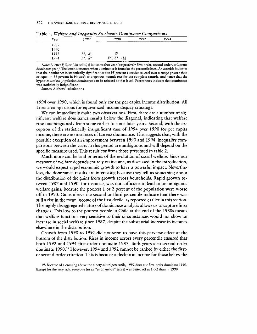
s22 THE WORLD BANK ECONOMIC REVIEW, VOL. 13, NO. 3
Table 4. Welfare and Inequality Stochastic Dominance ComparisonsYear 1987 1990 1992 1994
198719901992 F*, St S1994 F*, S* F*, S*, (L)
Note: A letter F, S, or L in cell (i, j) indicates that year i respectively first-order, second-order, or Lorenzdominates year j. The letter is inserted when dominance is found at the percentile level. An asterisk indicatesthat the dominance is statistically significant at the 95 percent confidence level over a range greater thanor equal to 99 percent in Howes's endogenous bounds test for the complete sample, and hence that thehypothesis of no population dominance can be rejected at that level. Parentheses indicate that dominancewas statistically insignificant.
Source: Authors' calculations.
1994 over 1990, which is found only for the per capita income distribution. AllLorenz comparisons for equivalized income display crossings.
We can immediately make two observations. First, there are a number of sig-nificant welfare dominance results below the diagonal, indicating that welfarerose unambiguously from some earlier to some later years. Second, with the ex-ception of the statistically insignificant case of 1994 over 1990 for per capitaincome, there are no instances of Lorenz dominance. This suggests that, with thepossible exception of an improvement between 1990 and 1994, inequality com-parisons between the years in this period are ambiguous and will depend on thespecific measure used. This result confirms those presented in table 2.
Much more can be said in terms of the evolution of social welfare. Since ourmeasure of welfare depends entirely on income, as discussed in the introduction,we would expect rapid economic growth to have a powerful impact. Neverthe-less, the dominance results are interesting because they tell us something aboutthe distribution of the gains from growth across households. Rapid growth be-tween 1987 and 1990, for instance, was not sufficient to lead to unambiguouswelfare gains, because the poorest 1 or 2 percent of the population were worseoff in 1990. Gains above the second or third percentile indicate that there wasstill a rise in the mean income of the first decile, as reported earlier in this section.The highly disaggregated nature of dominance analysis allows us to capture finerchanges. This loss to the poorest people in Chile at the end of the 1980s meansthat welfare functions very sensitive to their circumstances would not show anincrease in social welfare since 1987, despite the substantial increase in incomeselsewhere in the distribution.
Growth from 1990 to 1992 did not seem to have this perverse effect at thebottom of the distribution. Rises in income across every percentile ensured thatboth 1992 and 1994 first-order dominate 1987. Both years also second-orderdominate 1990.19 However, 1994 and 1992 cannot be ranked by either the first-or second-order criterion. This is because a decline in income for those below the
19. Because of a crossing above the ninety-ninth percentile, 1992 does not first-order dominate 1990.Except for the very rich, everyone (in an "anonymous" sense) was better off in 1992 than in 1990.

Ferreira and Litchfield 523
eighth or ninth percentile (which was sufficient to lower the mean income of thefirst decile, as discussed earlier) co-existed with gains for all other social groups.This welfare loss to the very poor means that we cannot say unambiguously thatsocial welfare rose over the last two years in our sample. The loss was not suffi-cient, however, to outweigh gains to those at the bottom of the distribution since1990: 1994 does first-order dominate both 1987 and 1990.
These results add rigor to our earlier analysis and broadly support its findings.The first fundamental feature of the period is economic growth, which led towelfare dominance of the last two years over the first two. On two occasions,however, economic growth failed to improve measured living standards for themost vulnerable people in society: from 1987 to 1990 and, more famously, from1992 to 1994. For these two periods we cannot make such an unambiguouswelfare comparison.
The second fundamental feature-the relative stability in the dispersion of thedistribution, but with a slight compression at the bottom and a stretching at thetop-is also compatible with the absence of significant Lorenz dominance re-sults. Such changes in the shape of the density function, reducing distances in onepart of the distribution while increasing them elsewhere, is exactly what causesdifferent inequality indexes to rank distributions in opposite ways. Although thissection emphasizes that the evidence on inequality is not sufficiently clear toidentify any real tendency in either direction, so that the most appropriate de-scription is one of broad stability or inconclusive changes, the (insignificant) Lorenzdominance of 1994 over 1990 for the per capita income distribution suggeststhat, if one were pushed to indicate a tentative direction for change in inequalityover the period, it would more likely be downward.
III. THE EVOLUTION OF POVERTY
The high GDP growth rates that Chile achieved over this period undeniablycontributed to a considerable reduction in poverty from the relatively high levelsof the mid-1980s. In this section we present detailed results on the changes in theincidence of poverty between 1987 and 1994, relying on our adjusted data setand comparing the numbers for household per capita income with those for house-hold income per equivalent adult. Although the general downward trend con-firms previous findings (see, for example, Larranaga 1994 and Contreras 1995),these new numbers reflect our adjustments, such as the incorporation of regionalprice differences, the adoption of a new equivalence scale, and the improvedtreatment of domestic servants (see appendix A). Before presenting the specificresults, we briefly discuss the derivation of the poverty lines, with respect towhich all of the measures must be understood.
We use three poverty lines in this study, all of them expressed in 1994 Santiagopesos per month: an indigence line set at P$15,050, a lower-bound poverty line(L) set at P$30,100, and an upper-bound poverty line (H) equal to P$34,164.The first two are the official indigence and poverty lines widely used in Chile.

524 THE WORLD BANK ECONOMIC REVIEW, VOL. 13, NO. 3
The incomes against which we compare them, however, differ from most earlierstudies in that we have "converted" them to 1994 Santiago pesos, using as an"exchange rate" the regional price index in table A-1 and the November con-sumer price index The derivation of the upper-bound line is explained below.
All three lines are absolute poverty lines, deriving from a standard food basketspecified by CEPAL. The basket is chosen so as to provide 2,187 Kcal per personper day, the national average caloric requirement, which is obtained from thedemographic characteristics of the population and from the Food and Agricul-ture Organization/World Health Organization recommended caloric intakes fordifferent age and gender groups. The specific commodity composition of the bas-ket is based on the actual consumption patterns of a reference group chosen byCEPAL. The reference group is the third quintile, measured according to consump-tion expenditures, in the Household Expenditure Survey of 1987-88. It is valuedat average prices for November 1994 in Santiago. The monthly cost of thisstandard CEPAL food basket has traditionally been used in Chile as an indigence(or extreme poverty) line, separating the hard-core poor-those whose currentmonthly incomes are insufficient even to purchase a minimum diet-from therest of society. In 1994 this amount was P$15,050, which we report below as theindigence line.
International practice, however, deems the indigence line too strict a criterionto identify the poor. There are, after all, other basic expenditures in addition tofood that everyone must make, such as shelter, clothing, and public transport.We apply a standard methodology to arrive at a sensible poverty line: we multi-ply the cost of the food basket by the inverse of the share of food in total expen-ditures (the Engel coefficient) for some suitable reference group. Based on theestimates of the Engel coefficient for the lower quintiles of the Chilean expendi-ture distribution, (reported in table 5), we adopt the standard value of 0.5, whichimplies a doubling of the indigence line, to arrive at the poverty line.20 However,although table S is reassuring in that the coefficients vary little from total house-hold expenditures to expenditures per capita (suggesting robustness with respectto the equivalence scale adopted), they are substantially lower for the concept ofper capita income including imputed rent. Since this is the welfare concept thatwe adopt for a large part of our analysis, we feel that we cannot ignore its impli-cations for poverty measurement.2 ' Weighing the relevant coefficients for thefirst and second quintiles by 0.8 and 0.2, respectively, we derive an Engel coeffi-cient of approximately 0.44. Applying its inverse (2.27) to the cost of the foodbasket yields our upper-bound poverty line (H) of P$34,164.
We also use the same three lines discussed above when computing povertymeasures using the vector of real household incomes per equivalent adult. Givenour choice of two-adult households as the reference type, the per capita poverty
20. Doing so has the important advantage of allowing some comparability with the findings of earlierstudies, most of which have used this line.
21. We also could not ignore it since the household income per equivalent adult concept also includesimputed rents.

Ferreira and Litchfield 525
Table 5. Engel CoefficientsIncome per capita
Quintile Total expenditures Expenditures per capita (including imputed rent)
1 0.530 0.539 0.4512 0.494 0.489 0.397
Source: CEPAI. (1996, p. 31, table 13).
line is unchanged for that household type. As with any equivalence scale de-signed to take account of different relative costs of children and of economies ofscale, ours implies different per capita poverty lines for household types otherthan the reference. This reflects the re-ranking of households that the scale inher-ently causes. Table 6 sets out what our equivalence scale implies in terms of house-hold and per capita poverty lines.
Let us now turn to the poverty measures. For a given poverty line, z, we candefine different poverty indexes, each aggregating information on the living stan-dards of those below the poverty line in different ways. We work with three ofthe most common measures, all of which can be expressed as members of thefollowing parametric class, proposed by Foster, Greer, and Thorbecke (1984):
(7) P. m X raxK 3'-"O]n " ' ( ) 0,
where y, is the income of the ith individual (of which there are n). The Foster-Greer-Thorbecke (FGT) measures are rather intuitive. As is well known, whenax = 0, P simplifies to pln, the headcount index. When cc = 1, we get the normal-ized poverty deficit, and ax = 2 yields the FGT(2) measure, which incorporatessome convexity to the distances between incomes and the poverty line, and ishence sensitive to inequality among the poor. Table 7 lists the values of each ofthese measures for the whole country, in each relevant year, for the distributionof household per capita income. Each index is listed for each of the three poverty
Table 6. Implied Household and Per Capita Poverty LinesEquivalence Household Implied per
Household type factor poverty linea capita poverty lineb
Single Adult 1.2 36,120 36,120Couple 2.0 60,200 30,100Couple + Child (age 0-4) 2.3 69,230 23,077Couple + Child (age 5-10) 2.4 72,240 24,080Couple + Child (age 11-15) 2.8 84,280 28,093Couple + Child (age 0-4) +
Child (age 11-15) 3.1 93,310 23,328
a. Equivalence factor x 30,100 = household poverty line.b. Household poverty line / number of persons = implied per capita poverty line.Source: Authors' calculations.
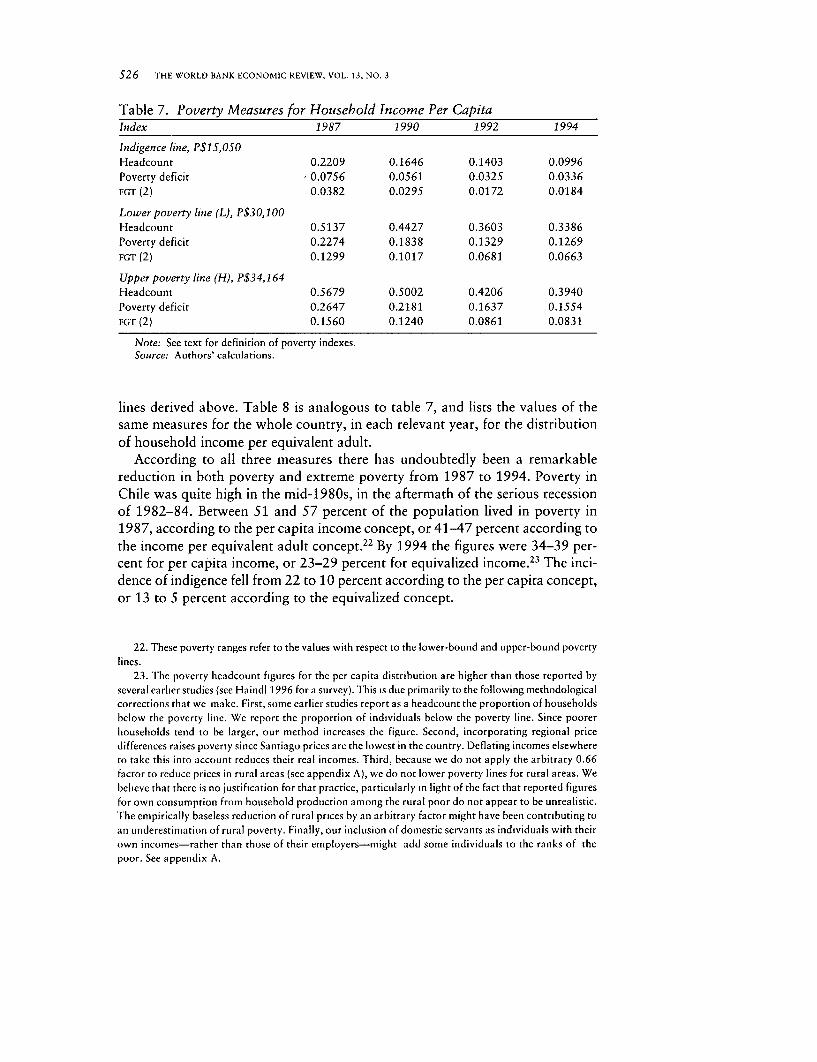
526 THE WORLD BANK ECONOMIC REVIEW, VOL. 13, NO. 3
Table 7. Poverty Measures for Household Income Per CapitaIndex 1987 1990 1992 1994
Indigence line, PS 15,050Headcount 0.2209 0.1646 0.1403 0.0996Poverty deficit 0.0756 0.0561 0.0325 0.0336FGT (2) 0.0382 0.0295 0.0172 0.0184
Lower poverty line (L), P$30,100Headcount 0.5137 0.4427 0.3603 0.3386Poverty deficit 0.2274 0.1838 0.1329 0.1269FGI' (2) 0.1299 0.1017 0.0681 0.0663
Upper poverty line (H), P534,164Headcount 0.5679 0.5002 0.4206 0.3940Poverty deficit 0.2647 0.2181 0.1637 0.1554FG'r (2) 0.1560 0.1240 0.0861 0.0831
Note: See text for definition of poverty indexes.Source: Authors' calculations.
lines derived above. Table 8 is analogous to table 7, and lists the values of thesame measures for the whole country, in each relevant year, for the distributionof household income per equivalent adult.
According to all three measures there has undoubtedly been a remarkablereduction in both poverty and extreme poverty from 1987 to 1994. Poverty inChile was quite high in the mid-1980s, in the aftermath of the serious recessionof 1982-84. Between 51 and 57 percent of the population lived in poverty in1987, according to the per capita income concept, or 41-47 percent according tothe income per equivalent adult concept. 22 By 1994 the figures were 34-39 per-cent for per capita income, or 23-29 percent for equivalized income.23 The inci-dence of indigence fell from 22 to 10 percent according to the per capita concept,or 13 to 5 percent according to the equivalized concept.
22. These poverty ranges refer to the values with respect to the lower-bound and upper-bound povertylines.
23. The poverty headcount figures for the per capita distribution are higher than those reported byseveral earlier studies (see Haindl 1996 for a survey). This is due primarily to the following methodologicalcorrections that we make. First, some earlier studies report as a headcount the proportion of householdsbelow the poverty line. We report the proportion of individtials below the poverty line. Since poorerhouseholds tend to be larger, our method increases the figure. Second, incorporating regional pricedifferences raises poverty since Santiago prices are the lowest in the country. Deflating incomes elsewhereto take this into account reduces their real incomes. Third, because we do not apply the arbitrary 0.66factor to reduce prices in rural areas (see appendix A), we do not lower poverty lines for rural areas. Webelieve that there is no justification for that practice, particularly in light of the fact that reported figuresfor own consumption from household production among the rural poor do not appear to be unrealistic.The empirically baseless reduction of rural prices by an arbitrary factor might have been contributing toan underestimation of rural poverty. Finally, our inclusion of domestic servants as individuals with theirown incomes-rather than those of their employers-might add some individuals to the ranks of thepoor. See appendix A.
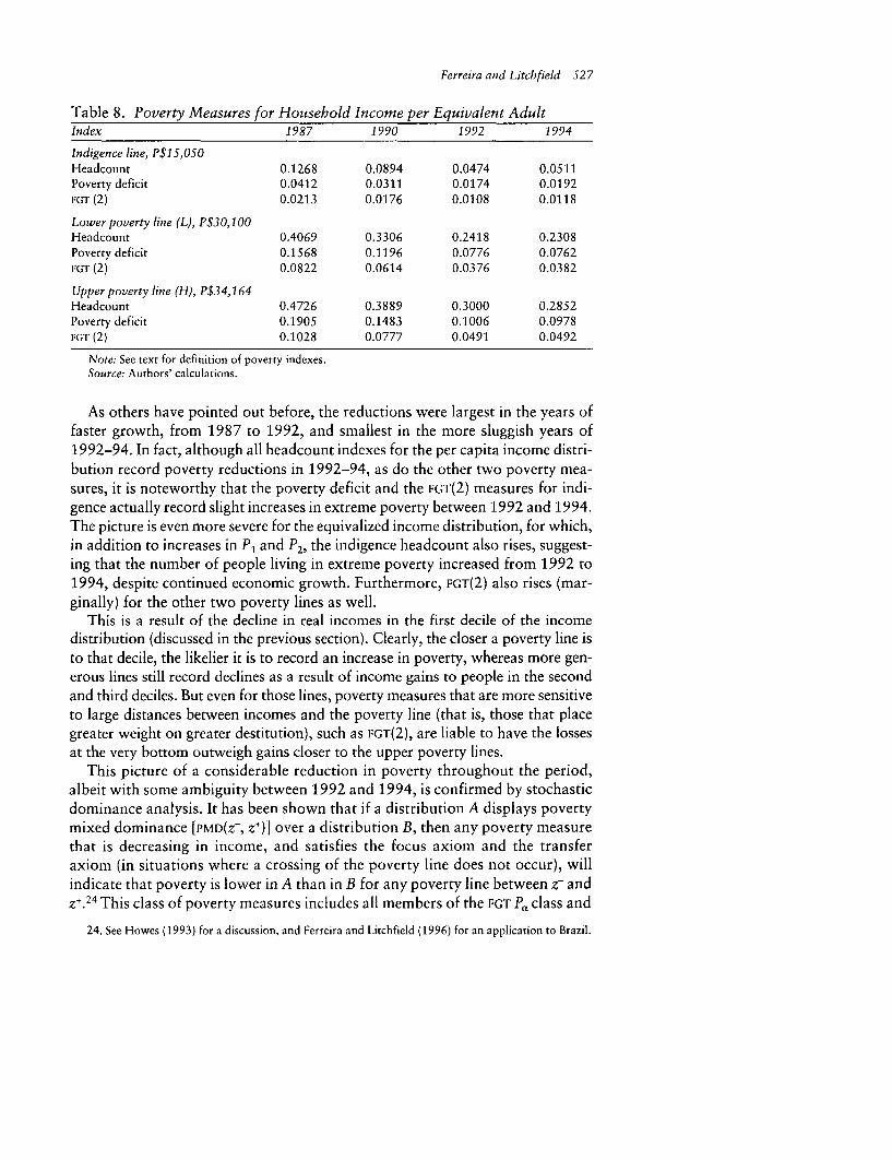
Ferreira and Litchfield 527
Table 8. Poverty Measures for Household Income per Equivalent AdultIndex 1987 1990 1992 1994
Indigence line, P$15,050Headcount 0.1268 0.0894 0.0474 0.0511Poverty deficit 0.0412 0.0311 0.0174 0.0192FGT (2) 0.0213 0.0176 0.0108 0.0118
Lo wer poverty line (L), P$30,100Headcount 0.4069 0.3306 0.2418 0.2308Poverty deficit 0.1568 0.1196 0.0776 0.0762FGT (2) 0.0822 0.0614 0.0376 0.0382
Upper poverty line (H), P$34,164Headcount 0.4726 0.3889 0.3000 0.2852Poverty deficit 0.1905 0.1483 0.1006 0.0978FGT (2) 0.1028 0.0777 0.0491 0.0492
Note: See text for definition of poverty indexes.Souirce: Authors' calculations.
As others have pointed out before, the reductions were largest in the years offaster growth, from 1987 to 1992, and smallest in the more sluggish years of1992-94. In fact, although all headcount indexes for the per capita income distri-bution record poverty reductions in 1992-94, as do the other two poverty mea-sures, it is noteworthy that the poverty deficit and the FGT(2) measures for indi-gence actually record slight increases in extreme poverty between 1992 and 1994.The picture is even more severe for the equivalized income distribution, for which,in addition to increases in P1 and P2, the indigence headcount also rises, suggest-ing that the number of people living in extreme poverty increased from 1992 to1994, despite continued economic growth. Furthermore, FGT(2) also rises (mar-ginally) for the other two poverty lines as well.
This is a result of the decline in real incomes in the first decile of the incomedistribution (discussed in the previous section). Clearly, the closer a poverty line isto that decile, the likelier it is to record an increase in poverty, whereas more gen-erous lines still record declines as a result of income gains to people in the secondand third deciles. But even for those lines, poverty measures that are more sensitiveto large distances between incomes and the poverty line (that is, those that placegreater weight on greater destitution), such as FGT(2), are liable to have the lossesat the very bottom outweigh gains closer to the upper poverty lines.
This picture of a considerable reduction in poverty throughout the period,albeit with some ambiguity between 1992 and 1994, is confirmed by stochasticdominance analysis. It has been shown that if a distribution A displays povertymixed dominance [PMD(Z-, Z+)] over a distribution B, then any poverty measurethat is decreasing in income, and satisfies the focus axiom and the transferaxiom (in situations where a crossing of the poverty line does not occur), willindicate that poverty is lower in A than in B for any poverty line between z andz+.24 This class of poverty measures includes all members of the FGT Pca class and
24. See Howes (1993) for a discussion, and Ferreira and Litchfield (1996) for an application to Brazil.

528 THE WORLD BANK ECONOMIC REVIEW, VOL. 13, NO. 3
Table 9. Poverty Mixed Stochastic Dominance ComparisonsYear 1987 1990 1992 1994
198719901992 P P1994 P P
Note: The letter P in cell (i, j) indicates that year i dominates year j.Source: Authors' calculations.
is therefore particularly appropriate for this study. Poverty mixed dominanceessentially requires that distribution A display second-order dominance over Bfrom zero to the lower-bound poverty line (z-), and first-order dominance fromz-to z+. Table 9, which is analogous to table 4, presents the results for Chile,with z- set at the indigence line and z+ set at the upper-bound poverty line (H).As before, we checked dominance for both per capita income and income perequivalent adult; both concepts yield exactly the same results.
These results reveal that there was unambiguously less poverty in 1992 and in1994 than in either 1987 or 1990, whether poverty is measured by the headcount,the poverty deficit, or indeed any of a host of other sensible poverty measures,and for any poverty line set between P$15,050 and P$34,164 per month in 1994Santiago pesos. This sort of unambiguous poverty reduction, independent of thespecific measure used and valid for such a large range of poverty lines, is notcommon. Its achievement confirms the widely held view that Chile has madesubstantial strides in the fight against poverty during the past decade.25
Yet there is also confirmation that growth did not lead to unambiguous pov-erty reductions in two subperiods: from 1987 to 1990 and from 1992 to 1994.On both occasions, although the headcount for the headline poverty line indi-cates a reduction in the number of poor people, there were income losses in thelowest percentiles of the distribution. These losses imply that some poverty mea-sures in the wide class defined above would indicate increases in poverty for atleast some of the poverty lines in the covered range. Indeed, in 1992-94 this wasthe case for all three indigence measures reported in table 8, for the equivalizedincome distribution. Still, the dominance of 1994 over both 1987 and 1990 indi-cates that the losses to some of the poor in the last two years were at least notsufficient to outweigh the gains made between 1990 and 1992.
Overall, there is no question that Chile's growth and social policies were tre-mendously successful in reducing the incidence, intensity, and inequality of pov-erty between 1987 and 1992, with the poverty deficits being roughly halved acrossall three poverty lines (a little less for per capita income, a little more for equivalized
25. All but one of the positive dominance results reported in table 9 follow directly from the first-orderdominances reported in table 4. Table 9 contains new information only for the cases in which there was nodominance, as well as for the dominance of 1992 over 1990, the distribution functions of which clearly do
not cross between z- and zl.

Ferreira and Litch field 529
income).26 The recent reversal in the performance of the poorest of the po6r,between 1992 and 1994, does, however, provide a cautionary signal againstcomplacency. 2 7
IV. CONCLUSIONS
In presenting an overview of welfare, inequality, and poverty trends in Chileduring 1987-94, this article has sought to establish a number of empirical con-clusions that can be drawn with confidence from a careful treatment of the data.These can be summarized as follows. Chilean inequality is high by internationalstandards, and it remained largely unchanged between 1987 and 1994. Scalarinequality measures-such as the Gini coefficient and the Theil index-variedlittle over the period, and there were no statistically significant Lorenz domi-nances between any of the years in the sample.
Within this broad picture of stability in inequality, however, there is someevidence that the shape of the density function may have altered slightly, with acompression at the lower tail (reducing bottom-sensitive inequality measures suchas the mean log deviation), and an increase in dispersion at the upper tail (leadingto rises in top-sensitive measures such as the coefficient of variation).
Economic growth has had a substantial and clearly beneficial impact, helpingshift the distribution function to the right. Welfare, as measured by any reason-able social welfare function, was unambiguously higher in both 1992 and 1994than it had been in either 1987 or 1990. Similarly, poverty was incontrovertiblylower. The bulk of these welfare improvements took place between 1987 and1992, however, and the slowdown in growth and increase in unemployment af-ter 1992 were associated with losses to the poorest 8 or 9 percent of the popula-tion. Although other social groups-including many of the poor-continued togain, the losses at the very bottom of the distribution were associated with anincrease in indigence between 1992 and 1994. Over the whole period, however,growth and other factors led to a remarkable decline in poverty, however it ismeasured, and for a wide range of plausible poverty lines. For some of theselines, headcounts and poverty deficits were halved from 1987 to 1994.
Although we have found that some assumptions underlying previous studiescontributed to underestimating both poverty and inequality-whether by arbi-trarily reducing prices when calculating poverty lines for rural areas, taking house-holds rather than individuals as the unit of analysis, or ignoring live-in domestic
26. Larranaga (1994) decomposes the changes in poverty in Chile between 1987 and 1992 into agrowth and a redistribution component, using a methodology of Datt and Ravallion (1992). Although hefinds that some 80 percent of the reduction could be explained by the effects of growth, some of thechanges were also due to a redistribution effect, which may have followed-at least in part-from thegovernment's social policies and expenditures.
27. Although the unit record data set of the CASEN 1996 was not made available for this study, thetabulated findings reported by MIDEPLAN (1997) suggest that faster growth after 1994 led to a resumptionof previous rates of poverty reduction and that inequality remained broadly stable.

530 THE WORLD BANK ECONOMIC REVIEW, VOL. 13, NO 3
servants-another important adjustment made in this study goes in the oppositedirection, suggesting that previous reports may have overestimated poverty andinequality. We have found that both poverty and inequality measures for Chileare considerably reduced when household income is adjusted to take into ac-count differences in needs between children and adults, and to take into accounteconomies of scale inherent in the sharing of fixed costs within the household.
Space constraints prevented us from investigating the determinants of the struc-ture of and the changes in inequality in Chile in this article. However, our previ-ous work suggests that education is by far the most important candidate vari-able. Ferreira and Litchfield (1998) find that differences between groups partitionedby educational attainment explain a much greater share of overall inequalitythan do differences in any other household attribute, and that changes in returnsto education appear to lie behind the reduction in bottom-sensitive inequalitymeasures over the period (see also World Bank 1997).
In that paper we argue that the importance of increases in education and thestability of overall inequality, taken together, also suggest that Chile may havereached a dynamic equilibrium between rising demand for and supply of skills.This would explain the recent reversal (or flattening) of the upward trend in bothearnings and personal income dispersion that other authors had identified forperiods prior to 1990. With the profound political and economic changes of the1970s and 1980s behind it, and regardless of its trade patterns, Chile's incomedistribution is, for the moment, calm.
APPENDIX A. THE DATA SET
The CASEN sampling methodology can be described as multi-stage randomsampling with geographical stratification and clustering. The country is firstdivided into strata comprising the rural and urban sectors of each of the 13regions.2 8 The rural sectors are final-level strata. The urban sectors are furthersubdivided into three categories of towns, according to population: towns withbetween 2,000 and 9,999 inhabitants; towns with between 10,000 and 39,999inhabitants; and towns with 40,000 or more inhabitants. All of the latter aresampled (that is, they are final-level strata). For other towns there is a level ofclustering in the selection of towns for sampling. At this level, with selectedsmall towns, all large towns, and the rural sectors, a first stage samples primaryunits (zonas de empadronamiento), with probabilities proportional to the popu-lation. A second stage samples households. This process is described in moredetail in annex III to MIDEPLAN (1992). The sample sizes for our analysis are asfollows: the 1987 sample includes 23,403 households; the 1990 sample con-sists of 26,248 households; the 1992 sample numbers 36,587 households; andthe 1994 sample covers 45,993 households.2 9
28. For this purpose an urban area is any grouping of dwellings with a population in excess of 2,000.29. These sample sizes are slightly larger than those reported in the official MIDEPLAN records of the
surveys, reflecting our treatment of live-in domestic servants as separate households. See below.

Ferreira and Litchfield 531
Once each survey is completed, the data are entrusted to CEPAL, which con-ducts two types of adjustments to the raw figures. The first type corrects for non-responses, which are made in three instances: when people who declare them-selves employed report no income from their main occupation, when people whostate that they receive an occupational or widow's pension do not report a valuefor this benefit, or when owner-occupiers of their domiciles do not report a valuefor imputed rent. In all three cases missing income values are replaced by theaverage value of the specific income variable in the group to which the householdbelongs, where the group is defined by a partition according to a number ofvariables, including region, gender of household head, educational attainment ofhousehold head, occupational sector, and category. See appendix 1 to CEPAL (1995)for details.
The second type of adjustment seeks to correct for underreporting oroverreporting of different income categories, a common problem with householdincome surveys everywhere. For this purpose CEPAL uses as the reference pointfor aggregate income flows the Household Incomes and Expenditures Accountof the National Accounts System (SCN) of the Central Bank of Chile. First, by acareful process the information in the original Central Bank accounts is con-verted to the income concepts surveyed by CASEN. Once that is achieved, totals byspecific income category are compared for CASEN (with recourse to the appropri-ate expansion weights) and the national accounts. Finally, the proportional dif-ferences for each income category between the two sources are imputed uni-formly to each income recipient in CASEN, with two notable exceptions: theadjustment in capital incomes is applied only to the top quintile (of households),proportionally to the primary incomes (ingresos autonomos) of all recipients there;and incomes from entitlement transfers and gifts are not adjusted. 30 The underly-ing assumption justifying this procedure is that misreporting differs fundamen-tally across income categories, rather than income levels.31 In fact, the imputa-tion would be strictly correct only if the income elasticity of misreporting withineach income category was unitary. The only exception to this assumption, asnoted, is in the treatment of capital incomes, which are imputed proportionally,but exclusively within the richest 20 percent of households. A detailed account ofCEPAL's adjustment methodology, complete with the numbers used in each of thefour years, is available in CEPAL (199S).
We also make three adjustments to the data set after it is processed by CEPAL.
The income variable from the CASEN records on which our analysis is primarilybased is total adjusted household income (YTOTHAJ), which includes all primary
30. It is suggested that the main reason for not adjusting entitlement transfers and gifts is that under-reporting of transfers consists mostly of complete omissions of benefits by some households, rather thanproportional underreporting of values by all recipients. There being no way to identify which householdsare omitting this information, no adjustment was found that would have improved the picture obtainedfrom the survey.
31. It may be interesting to note that the proportional adjustments do vary substantially across incomecategories. In fact, imputed rents are consistently found to have been overreported and are adjusteddownward in every survey.
532 THE WORLD BANK ECONOMIC REVIEW, VOL. 13, NO. 3
income, monetary transfers,3 2 and gifts, as well as imputed rent, after the CEPAL
adjustments. 3 3 It is from this variable that we construct both of the income con-cepts listed above-household income per capita and household income per equiva-lent adult-by appropriate choice of denominator. Our first adjustment is in thetreatment of live-in domestic servants. It is unclear how previous studies treatedthem, since YTOTHAJ is defined to exclude their incomes. Household-based stud-ies are likely to have unwittingly excluded them from the sample altogether, bysimply imputing YTOTHAJ to the household. For this article, in households withlive-in domestic servants, all other members received YTOTHAJ divided by theappropriate denominator (their number in the per capita income case, or theequivalence scale defined over them), while the servants were treated as a sepa-rate household whose income was the sum of total adjusted individual incomes(YTOTHIAJ) over them.
The second adjustment is to exclude from the analysis the three richest house-holds in the 1994 sample. This decision was carefully considered, and was basedon the impression that these households reported sufficiently disproportionateincomes to be regarded as genuine outliers. 34 This impression was reinforced bythe fact that two of these households were identical in every respect, having clearlybeen double-sampled, 35 and by the position of the three households as outliers ina plot of the Pareto distribution of the top 1 percent of the sample.
The third adjustment, as described in section I, is to deflate all incomes by aregional price index. The values of the regional deflators are given in table A-1.
32. We believe that the questionnaire coverage of monetary transfers from the state, whether at thefederal or municipal level, is exhaustive. Questions are asked and amounts are registered for the followingbenefits: Asignaciones Familiares, PASIS, SUF, Subsidio al Consumo de Agua Potable, and Subsidio de Cesantia.See MIDEPLAN (1996) for a description of each of these entitlement benefits. Other benefits, associated withformal employment, such as jubilaciones, pensiones de invalidez, and montepios are also included, althoughthey are aggregated as part of primary, rather than secondary, income.
33. We would have liked to use an even broader income concept, which takes into account the valuesof the transfers in-kind that the government makes to many households through programs in the areas ofeducation, health, and housing. Monitoring these expenditures is in fact one of the objectives of the CASFN,
and an exercise of valuation of these benefits is carried out by MIDEPLAN, relying on answers to surveyquestions about the usage of services and on cost data provided by the relevant ministries. Although themethodology for these valuations is discussed in MIDEPLAN (1993) and a tabulation of the imputations isavailable for quintiles of households in MIDEI'LAN (1994), the disaggregated imputations at the householdlevel-which would have been necessary for our analysis-are not made available with the other CASEN
variables. This is due to alleged problems of methodology and reliability. The results are therefore onlyavailable at the quintile level, for distributions of households, and are of very limited comparability withthe distributions used in this study. One should bear in mind that the-often substantial-value of theseservices, many of which are targeted, is omitted from the income data, when interpreting the distributionalresults that follow, or attempting to draw any conclusions about the social policies followed during the
period.34. The value of E(2)-see below-when the outliers are included, is 6.58 in 1994. Its range over the
other years is from 1.39 to 1.74.35. The practice of imputing all values from one household (randomly selected within the cluster) to
another when the latter has failed to respond, is often adopted as a way of maintaining representativenesswithin a small cluster. When the doubled household is the Rockefellers, the practice requires revision.

Ferreira and Litch field 533
Table A-1. Regional Price IndexesRegion Price index
I 1.2163II 1.1668Ill 1.1112IV 1.0859V 1.0420VI 1.0269VII 1.0136VIII 1.0441Ix 1.0500X 1.0383XI 1.0856XII 1.2208XIII (RM) 1.0000
APPENDIX B. INEQUALITY AND WELFARE ANALYSIS FOR PER CAPITA INCOMES
WITHOUT REGIONAL PRICE DEFLATION
Table B-1. Descriptive Statistics for Household Income Per Capita with NoRegional Price Adjustment
Statistic 1987 1990 1992 1994
Mean incomea 56,558 66,963 77,548 80,944Median income' 29,803 36,520 41,793 45,116Gini coefficient 0.5596 0.5523 0.5512 0.5429E(0) 0.5624 0.5444 0.5310 0.5219E(1) 0.6300 0.6401 0.6432 0.6079E(2) 1.3726 1.7297 1.6227 1.6468
a. In 1994 Santiago pesos.Note: See text for definition of statistics.Source: Authors' calculations.
Table B-2. Decile Income Shares for Household Income Per Capita with NoRegional Price Adjustment(percent)
Income category 1987 1990 1992 1994
Mean income(1994 Santiago pesos) 56,558 66,963 77,548 80,944
Decile 1 1.24 1.30 1.44 1.35Decile 2 2.20 2.33 2.39 2.36Decile 3 2.96 3.09 3.16 3.15Decile 4 3.78 3.93 3.94 4.00Decile 5 4.73 4.88 4.86 5.00Decile 6 5.95 6.12 6.09 6.26Decile 7 7.67 7.74 7.72 7.94Decile 8 10.41 10.25 10.19 10.65Decile 9 16.02 15.50 15.05 15.92Decile 10 45.04 44.85 45.16 43.36Top percentile 12.44 13.52 14.08 12.82
Source: Authors' calculations.
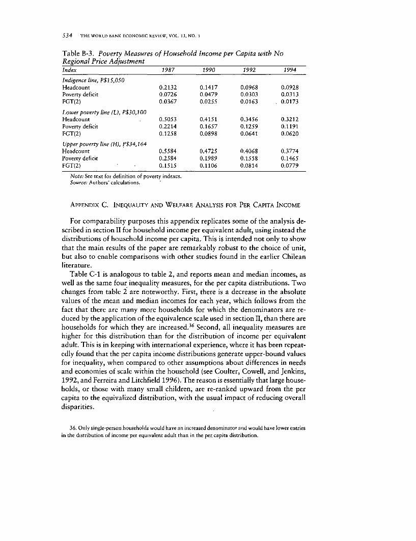
534 THE WORLD BANK ECONOMIC REVIEW, VOL. 13, NO. 3
Table B-3. Poverty Measures of Household Income per Capita with NoRegional Price AdjustmentIndex 1987 1990 1992 1994
Indigence line, P$15,00Headcount 0.2132 0.1417 0.0968 0.0928Poverty deficit 0.0726 0.0479 0.0303 0.0313FGT(2) 0.0367 0.0255 0.0163 . 0.0173
Lower poverty line (L), P$30,100Headcount . 0.5053 0.4151 0.3456 0.3212Poverty deficit 0.2214 0.1657 0.1259 0.1191FGT(2) 0.1258 0.0898 0.0641 0.0620
Upper poverty line (H), P$34,164Headcount 0.5584 0.4725 0.4068 0.3774Poverty deficit 0.2584 0.1989 0.1558 0.1465FGT(2) 0.1515 0.1106 0.0814 0.0779
Note: See text for definition of poverty indexes.Source: Authors' calculations.
APPENDIX C. INEQUALITY AND WELFARE ANALYSIS FOR PER CAPITA INCOME
For comparability purposes this appendix replicates some of the analysis de-scribed in section II for household income per equivalent adult, using instead thedistributions of household income per capita. This is intended not only to showthat the main results of the paper are remarkably robust to the choice of unit,but also to enable comparisons with other studies found in the earlier Chileanliterature.
Table C-1 is analogous to table 2, and reports mean and median incomes, aswell as the same four inequality measures, for the per capita distributions. Twochanges from table 2 are noteworthy. First, there is a decrease in the absolutevalues of the mean and median incomes for each year, which follows from thefact that there are many more households for which the denominators are re-duced by the application of the equivalence scale used in section II, than there arehouseholds for which they are increased. 36 Second, all inequality measures arehigher for this distribution than for the distribution of income per equivalentadult. This is in keeping with international experience, where it has been repeat-edly found that the per capita income distributions generate upper-bound valuesfor inequality, when compared to other assumptions about differences in needsand economies of scale within the household (see Coulter, Cowell, and Jenkins,1992, and Ferreira and Litchfield 1996). The reason is essentially that large house-holds, or those with many small children, are re-ranked upward from the percapita to the equivalized distribution, with the usual impact of reducing overalldisparities.
36. Only single-person households would have an increased denominator and would have lower entriesin the distribution of income per equivalent adult than in the per capita distribution.

Ferreira and Litchfield 535
Table C-1. Descriptive Statistics for Household Income Per CapitaIndicator 1987 1990 1992 1994
Mean incomea 55,367 63,293 75,371 78,281Median incomea 29,148 34,153 40,378 43,277Gini coefficient 0.5603 0.5563 0.5534 0.5454E(0) 0.5611 0.5495 0.5287 0.5212E(1) 0.6349 0.6509 0.6551 0.6194E(2) 1.3903 1.7447 1.6680 1.7121
a. In 1994 Santiago pesos.Note: See text for definition of the statistics.Source: Authors' calculations.
Despite those changes in level, there are no modifications to the perceivedtrends in inequality: the Gini still suggests a slight downward trend, but it isbasically stable. The Theil index, too, is trendless. The mean log deviation con-tinues to indicate a reduction in bottom-sensitive inequality, and the E(2) contin-ues to point to a gradual increase in top-sensitive inequality. This picture is broadlyconfirmed by the shares of each decile in the distribution of household incomeper capita, as revealed by table C-2.
Table C-2. Decile Income Shares for Household Income Per Capita(percent)
Income category 1987 1990 1992 1994
Mean income 55,367 63,293 75,371 78,281Decile 1 1.21 1.21 1.35 1.28Decile 2 2.19 2.26 2.35 2.33Decile 3 2.95 3.03 3.13 3.11Decile 4 3.77 3.87 3.91 3.96Decile 5 4.72 4.84 4.83 4.96Decile 6 5.94 6.07 6.05 6.22Decile 7 7.66 7.71 7.70 7.91Decile 8 10.37 10.25 10.18 10.60Decile 9 15.89 15.49 14.97 15.95Decile 10 45.30 45.26 45.63 43.66Top percentile 12.54 13.60 14.31 12.94
Source: Authors' calculations.

536 THE WORLD BANK ECONOMIC REVIEW, VOL. 13, NO. 3
REFERENCES
The word "processed" describes informally reproduced works that may not be com-monly available through library systems.
Atkinson, A. B. 1970. "On the Measurement of Inequality." Journal of Economic Theory2(3): 244-63.
Becker, Gary. S. 1965. "A Theory of the Allocation of Time." Economic Journal 75:493-517.
Beyer, H. 1995. "Logros en la Pobreza; Frustracion en la Igualdad?" Estudios Publicos60(1):15-33.
CEPAL (United Nations Economic Commission for Latin America and the Caribbean).1995. "La Medicion de los Ingresos en la Perspectiva de los Estudios de Pobreza: Elcaso de la Encuesta CASEN de Chile: 1987-1994." CEPAL Working Paper LC/R1604.Santiago. Processed.
.1996. "La Sensibilidad del Indicador de Pobreza." CEPAL Working Paper LC/R1657.Santiago. Processed.
Chauduri, Shubham, and Martin Ravallion. 1994. "How Well do Static Indicators Iden-tify the Chronically Poor?" Journal of Public Economics 53(3):367-94.
Comision Nacional dejusticia y Paz. 1996. "Es Chile un Pais Equitativo?" Area PastoralSocial de la Conferencia Episcopal de Chile. Santiago. Processed.
Contreras, Dante. 1995. "Poverty, Inequality and Welfare in Chile: 1987-1992." De-partment of Economics, Universidad de Chile. Processed.
Coulter, F. A. E, F. A. Cowell, and S. P. Jenkins. 1992. "Equivalence Scale Relativitiesand the Extent of Inequality and Poverty." Economic Journal 102(414):1067-82.
Cowan, K., and J. De Gregorio. 1996. "Distribucion y Pobreza en Chile: Estamos mal?Ha habido progresos? Hemos retrocedido?" Ministerio de Hacienda de Chile. Santiago.Processed.
Cowell, F.A. 1995. Measuring Inequality. Second Edition. Hemel Hempstead: HarvesterWheatsheaf.
Datt, Gustav, and Martin Ravallion. 1992. "Growth and Redistribution Components ofChanges in Poverty Measures." Journal of Development Economics 38(2):275-95.
Deaton, Angus. 1997. The Analysis of Household Surveys: Microeconometric Analysisfor Development Policy. Baltimore, Md.: The Johns Hopkins University Press.
Deininger, Klaus, and Lyn Squire. 1996. "A New Data Set Measuring Income Inequal-ity." The World Bank Economic Review 10(3):565-91.
Edwards, Sebastian, and A. C. Edwards. 1987. Monetarism and Liberalization: The Chi-lean Experiment. Chicago: University of Chicago Press.
Ferreira, Francisco H. G., and Julie A. Litchfield. 1996. "Growing Apart: Inequality andPoverty Trends in Brazil in the 1980s." LSE STICERD DARP Discussion Paper 23, Suntoryand Toyota International Centres for Economics and Related Disciplines, London Schoolof Economics, London.
. 1998. "Calm After the Storms: Income Distribution in Chile, 1987-1994." PolicyResearch Working Paper 1960, Development Research Group, World Bank, Wash-ington, D.C.
Foster, James. E., Joel Greer, and Erik Thorbecke. 1984. "A Class of DecomposablePoverty Measures." Econometrica 52(3):761-66.

Ferreira and Litchfield 537
Haindl, E. 1996. "Poverty and Income Distribution in Chile: A Survey." World Bank,Washington, D.C. Processed.
Howes, S. R. 1993. "Income Distribution: Measurement, Transition and Analysis of Ur-ban China, 1981-1990." Ph.D. dissertation, London School of Econormics.
Larranaga, Osvaldo. 1994. "Pobreza, Crecimiento y Desigualdad: Chile, 1987-1992."Revista de Analisis Economico 9(2):69-92.'
Londono, J. L., and M. Szekely. 1997. "Persistent Poverty and Excess Inequality: LatinAmerica during 1970-1995." Office of the Chief Economist, Inter-American Develop-ment Bank, Washington, D.C. Processed.
Marcel, M., and Andres Solimano. 1994. "The Distribution of Income and Economic Adjust-ment." In B. P. Bosworth, Rudiger Dombusch, and Raul Laban, eds., The Chilean Economy:Policy Lessons and Challenges. Washington, D.C.: The Brookings Institution.
Meller, P. 1996. "Trade Liberalization and Wage Differentials in Chile." Paper presentedat the XIV Latin American Econometric Society Meetings, Rio de Janeiro, August.Processed.
MIDEPLAN. 1992. Poblacion, Educacion, Vivienda, Salud, Empleo y Pobreza: CASEN 1990.
Santiago: Ministerio de Planificacion y Cooperacion..1993. Programas Sociales: Su impacto en los hogares chilenos, CASEN 1990. Santiago:
Ministerio de Planificacion y Cooperacion.___ .1994. Integracion al Desarrollo: Balance de la politica social, 1990-1993. Santiago:
Ministerio de Planificacion y Cooperacion.. 1996. Balance de Seis Anos de las Politicas Sociales: 1990-1996. Santiago:
Ministerio de Planificacion y Cooperacion.. 1997. "Pobreza y Distribucion del Ingreso en Chile, 1996: Resultados de la CASEN."
Santiago. Processed.Montenegro, C. 1996. "The Structure of Wages in Chile, 1960-1993: An Application of
Quantile Regressions." Inter-American Development Bank, Washington, D.C. Pro-cessed.
OECD (Organisation for Economic Co-operation and Development). 1982. The OECD Listof Social Indicators. Paris.
Ravallion, Martin, and Benu Bidani. 1994. "How Robust is a Poverty Profile?" TheWorld Bank Economic Review 8(1):75-102.
Riveros, L. 1983. "Distribucion del Ingreso en el Gran Santiago." Revista de Economia,9, Universidad de Chile.
Robbins, D. 1994. "Worsening Relative Wage Dispersion in Chile During Trade Liberal-ization and its Causes: Is Supply at Fault?" Harvard Institute for International Devel-opment, Cambridge, Mass. Processed.
. 1995. "Relative Wage Structure in Chile, 1957-1992: Changes in the Structure ofDemand for Schooling." Estudios de Economia 21(1):51-78.
____. 1996. "HOS Hits Facts: Facts Win. Evidence on Trade and Wages in the Develop-ing World." Harvard Institute for International Development, Cambridge, Mass. Pro-cessed.
Saposnik, R. 1981. "Rank-Dominance in Income Distribution." Public Choice 36(1):147-S1.
Scott, C. 1996. "The Distributive Impact of the New Economic Model in Chile." In V.Bulmer-Thomas, ed., The New Economic Model in Latin America and its Impact onIncome Distribution and Poverty. London: Macmillan.

538 THE WORLD BANK ECONOMIC REVIEW, VOL. 13, NO. 3
Sen, Amartya K. 1981. Poverty and Famines: An Essay on Entitlement and Deprivation.Oxford: Clarendon Press.
Shorrocks, A. F. 1983. "Ranking Income Distributions." Economica 50(1):3-17.UNDP (United Nations Development Programme). 1996. Desarrollo Humano en Chile,
1996. Santiago.Wood, Adrian. 1997. "Openness and Wage Inequality in Developing Countries: The Latin
American Challenge to East Asian Conventional Wisdom." The World Bank Eco-nomic Review 11(1):33-57.
World Bank. 1997. Chile-Poverty and Income Distribution in a High-Growth Economy:1987-1995. Report 16377-CH, Latin America and the Caribbean Region, Washing-ton, D.C.
THE WORLD BANK ECONOMIC REVIEW, VOL. 13, NO. 3: 539-59
Changes in the Perception of the Poverty LineDuring the Depression in Russia, 1993-96
Branko Milanovic and Branko Jovanovic
Economic transition in Russia was accompanied by a precipitous decline in real incomefor most of the population. This article analyzes how the decline affected people's per-ception of the minimum level of income needed to make ends meet. Individual-level datacollected from repeated surveys between March 1993 and September 1996 reveal thatthe elasticity of subjective minimum income with respect to actual median income was1.5 or that people's subjective estimate of the minimum income for an adult Russian fellabout 1.7 percent each month. This sharp reduction in the face of a decrease in realincome meant that the percentage of the population who felt that they were poor de-clined, even though poverty remained at a very high level (more than 60 percent of thepopulation) throughout the period. This self-perception is in marked contrast to an"objective" measure of poverty: the percentage of the population whose income was lessthan a given real poverty line rose.
In the course of its transition to a market system, the Russian economy experi-enced a series of shocks. Its output fell sharply: gross domestic product (GDP) in1997 was almost one-third less than it was in 1987. It suffered from rapid andcontinuing inflation: during the period under study here (March 1993 to Septem-ber 1996) the price level increased 46 times. Open unemployment appeared, af-fecting about 10 percent of the labor force by 1997. Real wages and pensionsdeclined to half their level before the transition, and delays in their paymentbecame endemic. A few individuals who were politically well connected, enter-prising, or lucky were able to amass considerable wealth. As a consequence, sincethe transition began, income inequality has risen by an unprecedented amount(the Gini coefficient increased four to five times faster in Russia than in the UnitedStates during the 1980s; see Milanovic 1998). The number of families living inpoverty also increased rapidly.'
Given these developments, the population's views about what constitutes pov-erty and the minimum income needed to "make ends meet" likely evolved aswell. Because the decline in income was so sharp, it reveals, within a very com-
1. See, for example, Braithwaite (1997); Glinskaya and Braithwaite (1998); Milanovic (1998); Lokshinand Popkin (1998); and Ovcharova, Turuntsev, and Korchagina (1998).
Branko Milanovic is with the Development Research Group at the World Bank, and Branko jovanovicis with the Economics Department at Texas A&M University and the Development Research Group at theWorld Bank. Their e-mail addresses are [email protected] and [email protected]. Theauthors gratefully acknowledge comments from Jeanine Braithwaite, Christine Jones, Misha Lokshin, andthree anonymous referees. The research was financed by World Bank research grant RPO 681-42.
© 1999 The International Bank for Reconstruction and Development/THE WORLD BANK
S39
540 THE WORLD BANK ECONOMIC REVIEW, VOL. 13, NO. 3
pressed time period, how conceptions of well-being and deprivation respond toabrupt changes in income (see, for example, Kahneman and Thaler 1991). Formost people in most countries these concepts remain relatively constant overconsiderable periods of time. It is therefore difficult to observe the impact ofchanges in external circumstances on the formation of attitudes or expectations.But the Russian experience allows us to do so. In addition, the question of whatthe population believes to be the minimum acceptable income has obvious politi-cal implications: if most people feel poor, they are unlikely to support reform.This article explores how the perception of the poverty line, among the popula-tion as a whole, changed in Russia during 1993-96.
I. THE MODEL
In the literature on subjective welfare estimation the usual specification de-fines the minimum income necessary for a family to make ends meet (MYf) as adependent variable. MYf may be considered a point on a household cost functionrelated to a specific level of welfare um i. In the most parsimonious formulationtotal household income (Yf) and family size (n) are explanatory variables (Goedhartand others 1977; Hagenaars and van Praag 1985; van Praag and Van der Saar1988):
(1) In MYf= fct(ln Yf, ln n).
The minimum income necessary for a family to make ends meet is obtainedfrom a so-called minimum-income question, such as "What do you consider asan absolute minimum net income (per period of time) for a household such asyours?" (see Flik and van Praag 1991). Obviously, family size positively influ-ences the minimum income or subjective poverty line-we use the terms inter-changeably. In addition, the actual level of family income, which may be re-garded as a proxy for the family's permanent income, positively influences thesubjective poverty line. The rationale is that families accustomed to a higherstandard of living will, everything else being the same, have higher aspirationsand hence a higher estimate of their minimum income. van Praag (1971) callsthis "the preference drift." Its value, in a double-log formulation such as equa-tion 1, lies between 0 and 1. If the preference drift equals 0, then the subjectivepoverty line becomes an absolute poverty line. At the other extreme, when thepreference drift equals 1, every increase in real income exacts the same percent-age increase in what is perceived to be the poverty line. The poverty line thenbecomes fully relative. Not surprisingly, most research has yielded values of thepreference drift between 0.4 and 0.7 (see, for example, Flik and van Praag 1991and van Praag and Flik 1992). These values fit well with our intuitive perceptionthat, as people get richer, they set the necessary minimum higher, but do not raiseit (in percentage terms) as much as the rise in their income.
Answers to the minimum-income question yield several observations. We fitthe regression based on these observations; the intersection of the regression and
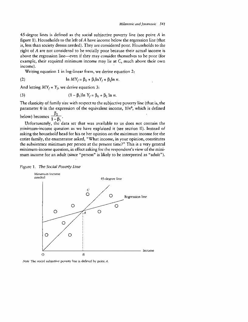
Milanovic and Jovanovic 541
45-degree lines is defined as the social subjective poverty line (see point A infigure 1). Households to the left of A have income below the regression line (thatis, less than society deems needed). They are considered poor. Households to theright of A are not considered to be socially poor because their actual income isabove the regression line-even if they may consider themselves to be poor (forexample, their required minimum income may lie at C, much above their ownincome).
Writing equation 1 in log-linear form, we derive equation 2:
(2) In MYf = 0 + 3llnYf + j321n n.
And letting MYf = Yf, we derive equation 3:
(3) (1- 01)lnYf= 00+ 0 2lnn.
The elasticity of family size with respect to the subjective poverty line (that is, theparameter 0 in the expression of the equivalent income, Yln/, which is defined
below) becomes 1 I2
Unfortunately, the data set that was available to us does not contain theminimum-income question as we have explained it (see section II). Instead ofasking the household head for his or her opinion on the minimum income for theentire family, the enumerator asked, "What income, in your opinion, constitutesthe subsistence minimum per person at the present time?" This is a very generalminimum-income question, in effect asking for the respondent's view of the mini-mum income for an adult (since "person" is likely to be interpreted as "adult").
Figure 1. The Social Poverty Line
Minimum incomeneeded 45-degree line
0 0 Regression line
0T
0 0/
Income0 B
Note The social subjective poverty line is defined by point A.

542 THE WORLD BANK ECONOMIC REVIEW, VOL. 13, NO. 3
It does not ask what the minimum income per person would be for that family.2Therefore, we cannot apply our theory in a straightforward fashion; we must usean alternative approach.
Equation 4 shows the effective formulation based on the question as askedand introduces other control variables that may be relevant:
(4) In AMY = fct(ln Y*# age, age2, SETTLEMENT, REGION, time).
AMY represents answers to the question about the minimum income for an adult.The other variables are Y* the true income level of the household (income perequivalent adult in the household), age of the respondent, size of the settlement(a dummy variable), region where the family lives (a dummy variable), and time.The crucial variable is true income. In trying to determine what people believe tobe the minimum income for an adult in Russia based on their own income, wemust define Y* so that it accurately reflects the household's economic welfare.Clearly, Y* is unlikely to be total family income because total family income doesnot take into account the number of people in the family. But it could be percapita income or income per equivalent adult, which accounts for economies ofsize. Therefore, we define Y* as Yin8, where 0 is a parameter for economies ofsize ranging from 0 (full economies of size) to 1 (no economies of size or percapita measurement).
Determining the right 0 is problematic. We argue that the right 0 (0*) willmake the sign of the, variable for household size (n) not significantly differentfrom 0. The rationale is as follows. Once we identify true household income,there is no reason why a household's size or composition should affect whatpeople regard as the minimum income for an adult. Therefore, we try differentvalues of Y(0') and choose the 0 = 0* that makes the coefficient on In n equal to0 in equation 3. For values of 0 < 0* we expect the coefficient on In n to benegative because the economic welfare of large households is overestimated (theyare not as rich as they seem). Their estimate of minimum income (AMY) is sys-tematically biased downward, which in turn leads to a negative correlation be-tween AMY and In n and to a negative regression coefficient. For values of 0 > 0*the opposite is true, and we expect the regression coefficient to be positive.
Including the age and age2 variables accounts for the (parabolic) life-cycle ef-fect whereby perceived needs increase until they reach a peak and decrease there-after. We have to be careful with the interpretation of these variables becausethey record the age of the respondent and not necessarily the age of the house-hold head.
We capture the importance of the environment on the perception of the pov-erty line by introducing a dummy variable for the size of the settlement and adummy variable for the region where the settlement is located. People living inbig cities or richer regions (for example, Moscow or St. Petersburg) face higher
2. If respondents are rational, there is no difference between asking them the minimum total incomefor their family and the minimum per capita income for their family. The answers to the latter can simplybe multiplied by the number of family members to obtain the minimum family income.

Milanovic and Jovanovic 543
prices and would be expected to pitch their poverty line higher.3 The social refer-ence (demonstration) effect may also be important in larger cities, as people see-ing the wealth of others come to expect more. Living in a harsh climate mightalso increase people's perception of the necessary minimum income.
Finally, we introduce a variable for time in our model in order to capturechanges in the perception of the poverty line over time. Our hypothesis is that thesubjective poverty line will fall as time passes and people adapt to worseningconditions. Our data span March 1993 to September 1996, during which timethe real income of the Russian population declined severely. The decline is esti-mated at 14 percent based on our survey results or at almost 20 percent based onofficial (Goskomstat) monthly estimates of population income over the sameperiod (see figure 2). Note from figure 2 that our data underestimate income byabout 40 percent compared with the official data, but also that the underestima-tion diminishes with time. Most of the difference is due to the omission of in-come in kind from the survey data. Both official and survey data almost certainlyunderestimate the gray or black economy.
We ask whether, in addition to the income effect, the passage of time and therealization of what seem to be ever-worsening circumstances lead the public toscale down its expectation of the minimum tolerable income. As adaptation toless-fortunate circumstances proceeds, we expect the time variable to enter nega-tively in equation 3.
II. THE DATA
We use the 29 cross-sectional data sets from the All-Russian Centre for PublicOpinion Research (vcIoM by its Russian abbreviation), covering the period fromMarch 1993 to September 1996. The survey is a representative sample of Rus-sian households. It was conducted monthly between March 1993 and January1994, and approximately every second month since then. Although most of thesurvey questions are concerned with the household (family), some questions tar-get individuals. These variables include, among others, gender, age, and educa-tion. In most surveys such questions are targeted specifically to the head of thehousehold. Here, however, the respondent is not necessarily the household head.The fact that the respondent need not be the household head might jeopardizethe accuracy of some data (for example, the respondent may not be fully awareof all the components of household income).
The original data set consisted of 91,090 observations spread over 29 crosssections. We reduced the number of observations to 80,826 after omitting thosethat did not contain information on family income (total or by components).Individual cross sections contained between 3,626 (January 1994) and 2,034(September 1996) observations. The reduction of the sample size over time was
3. Our database is not deflated for regional price differences because regional consumer price indexesare not available.

544 THE WORLD BANK ECONOMIC REVIEW, VOL. 13, NO. 3
Figure 2. Real Population Income, 1993-96(thousands of constant March 1993 rubles per capita per month)
Income40-
35 -
30-
25 -cpia income,
20-
15 - t Survey mean per: lI capita income
10-
5
1 1993 5 1994 9 1995 13 1996Quarters
Note: Broken lines show trends.Source: Survey per capita income calculated from VCJOM surveys. Official per capita income from monthly
Goskomstat statistics.
considerable; however, according to the VCIOM staff, it did not make the sampleless representative because the sampling procedures were improved.4
Table 1 gives summary statistics for the basic characteristics of the householdsand respondents surveyed. 5 Total family income is computed as the sum of in-come components: main income and income from a second job, private sectoractivities, pensions, other social transfers (including family, unemployment, anddisability benefits), stipends, alimony, income from financial papers (stocks andbonds, vouchers, interest from savings accounts), sale of self-produced goods,and other monetary income (appendix A provides details). We use the all-Russiamonthly consumer price index (cpl), with March 1993 as the base, to deflate allthe monetary variables. We assume that inflation affects all regions equally (re-gional cp'is are not available).
In real terms the subjective minimum income for an adult (AMY)--calculatedas an individual-'weighted average of AMYs over all households-decreased dra-matically between March 1993 and September 1996. It started out higher than
4. We owe this information to Jeanine Braithwaite.S. More detailed statistics are available from the authors.

Milanovic and jovanovic 54S
Table 1. Summary Descriptive Statistics, 1993-96Variable 1993 1994 1995 1996
Women (percent) 60.06 60.12 57.04 56.65Age of respondent (years) 42.71 42.40 42.58 43.29
Education attained by respondent (percent)Primary or less 6.10 5.85 5.82 5.51Secondary, incomplete 8.08 8.15 8.75 8.56Secondary, completed with no diploma 2.69 2.58 2.31 2.53Technical school, less than secondary 4.44 4.07 3.99 4.45Secondary, completed with diploma 15.34 14.88 15.16 13.79Technical school and secondary 9.80 10.22 9.87 10.29Vocational school 27.57 28.33 27.34 27.19University, 3-4 years 3.20 3.44 3.81 3.90University, completed 22.77 22.49 22.96 23.78
Number of observations 34,759 23,040 12,189 10,298
Note: Values are averages of the monthly averages, with 10 months for 1993, 8 months for 1994, 6months for 1995, and 5 months for 1996.
Source: Authors' calculations from the vcIoM data.
Rs35,000 (rubles) in the early surveys and ended at Rs15,000 (see figure 3). TheMinistry of Labor's official minimum income for an adult (prozhitochnyi mini-mum) remained constant in real terms at around Rs10,000. 6 The gap betweenthe subjective and the official minimum diminished steadily, as the public percep-tion of the minimum income for an adult Russian gradually approached the offi-cial minimum.
The composition of households, as well as the demographic characteristics ofthe respondents, stayed roughly the same over time (see tables 1 and 2). Over theentire survey period the average household consisted of 3.1 members, with 0.7children (table 2). For comparison, according to the all-Russia official statisticsfor 1994, the average household size was 2.84 members (Goskomstat Rossii 1995).The average survey respondent was 42.7 years old and spent 11.2 years in school(table 1). The average duration of schooling of the population over 15 years ofage calculated from the 1993 Russian Longitudinal Monitoring Survey was alittle over nine years. Of all the respondents, 59.2 percent were women; accord-ing to official statistics, women made up 53 percent of the Russian population in1995.
Most of the respondents (76.5 percent) lived in urban areas, a percentage closeto the official 1995 statistics (73 percent). A plurality of respondents (46 percent)lived in cities with populations less than 100,000, followed by 25.1 percent wholived in cities with populations over 1 million.
In order to check for possible outliers in the data, especially in Yf and AMY,we create a flag variable. We compute the variable for each cross section sepa-
6. The official minimum is composed of a given bundle of food and nonfood goods. Its slight oscillationsaround RslO,000 in March 1993 prices are due to the fact that the ci'i we use to deflate the nominalmonthly values of the official minimum at times might have increased faster or slower than the cost of theminimum bundle of goods.

546 THE WORLD BANK ECONOMIC REVIEW, VOL. 13, NO. 3
Figure 3. The Average Subjective Poverty Line for an Adult, the Official PovertyMinimum for an Adult, and Average Per Capita Income, 1993-96(thousands of March 1993 rubles per month)
Poverty lines, income
40
35
30
Subjective poverty line for an adult
25-
20-
15-
I Income per capita Official minimum income for
10 =
5.1 2 3 4 5 6 7 8 9 10 11 12 13 14 15 16 17 18 19 20 21 22 23 24 25 26 27 28 29
1993 1994 1995 1996Survey number
Note: The average subjective poverty line for an adult is the simple individual-weighted average ofpoverty lines (AMY) in the surveys; the official poverty line for an adult is the all-Russia official povertyline (MinTruda Rossii); the average per capita income is the average income from vcioM surveys (as infigure 2).
Source: Authors' calculations.
rately according to the method developed by Hadi (1992, 1994) using the hadimvoprocedure in STATA; 2,634 observations are identified as possible outliers, repre-senting 3.28 percent of the total sample.
III. ESTIMATING THE SUBJECTIVE POVERTY LINE
We first try to estimate true household income using different values of 0. Todo so, we run the basic model, equation 3, including in addition In n as thecontrol variable for household size. Figure 4 shows how the coefficient on In nchanges as 0 in Y(0*) varies from 0 to 1. For 0 = 0.62, the coefficient equals 0. (Itis insignificantly different from 0 for a few other values around 0.6, but takes itslowest value for 0 = 0.62.)
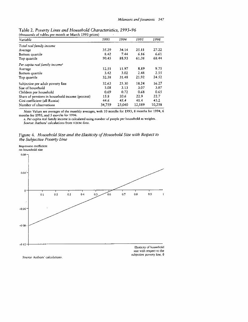
Milanovic and Jovanovic 547
Table 2. Poverty Lines and Household Characteristics, 1993-96(thousands of rubles per month at March 1993 prices)
Variable 1993 1994 1995 1996
Total real family incomeAverage 35.29 34.14 25.11 27.22Bottom quartile 8.42 7.44 6.16 6.61Top quartile 90.45 88.93 61.38 68.44
Per capita real family income&Average 12.51 11.97 8.89 9.75Bottom quartile 3.42 3.02 2.48 2.55Top quartile 32.38 31.48 21.92 24.52
Subjective per adult poverty line 32.63 25.30 18.24 16.27Size of household 3.08 3.13 3.07 3.07Children per household 0.69 0.72 0.68 0.65Share of pensions in household income (percent) 15.8 20.6 22.9 22.7Gini coefficient (all Russia) 44.6 45.4 41.4 45.2Number of observations 34,759 23,040 12,189 10,258
Note: Values are averages of the monthly averages, with 10 months for 1993, 8 months for 1994, 6months for 1995, and 5 months for 1996.
a. Per capita real family income is calculated using number of people per household as weights.Source: Authors' calculations from VCIOM data.
Figure 4. Household Size and the Elasticity of Household Size with Respect tothe Subjective Poverty Line
Regression coefficienton household size
0.08 -
0.04 -
0.1 o 2 0.3 0 4 o 0. 0.7 0.8 0.9
-0.04 -
-o 08-/
-0 12-Elasticity of household
size with respect to thesubjective poverty line, 0
Source Authlors' calculations.

s48 THE WORLD BANK ECONOMIC REVIEW, VOL. 13, NO. 3
We then directly estimate equation 3 using Y* = Y (table 3).7 All the re-N0q 62
gressions are run with Huber (robust) variances to adjust for the fact that theobservations are drawn from different time clusters (that is, from the 29 surveys).The Huber correction also adjusts for the fact that the variability of the observa-tions within each survey is less than it would be if all observations were ran-domly drawn from the population at large. That is, the variability of the observa-tions from the pooled cross sections is less than what it would be if all 80,000 ofour observations were drawn from one cross section. Nevertheless, the t-valuesin table 3 show that most of the coefficients are significant at a probability greaterthan 99 percent.
The elasticity of the subjective poverty line for an adult with respect to incomeis 0.144 for the overall sample and 0.132 in a regression that excludes Hadioutliers (see appendix B on the hadimvo procedure). These values are signifi-cantly lower than those reported by Frijters and van Praag (1994) in their studyof the former Soviet Union and Russia. Frijters and van Praag report preferencedrift values of 0.62 and 0.64 for Russia in 1993 and 1994, respectively. For theSoviet Union in 1991, they report a value of 0.41. However, our results and theirresults are not entirely comparable. Frijters and van Praag use a variant of the so-called income evaluation question in order to obtain the left-side variable (theLeyden poverty line).8 We use the income level that people consider the mini-mum value for an adult.
We calculate a value for preference drift that is significantly lower than the valuefound in some Western countries. Flik and van Praag (1991), for example, report avalue of 0.59 for the Netherlands. Hagenaars and van Praag (1985) report a valueof 0.54 for a collection of West European countries. Part of the difference may bedue to the richer choice of control variables included here (regional and size ofsettlement dummies), as well as to the introduction of the time variable. In effect, ifwe run a very parsimonious formulation, such as equation 1, which is basicallywhat Hagenaars and van Praag (1985) do (without a control variable for house-hold size), the preference drift increases from 0.14 to 0.23.
The latter value (0.23) is almost identical to the preference drift of 0.223 ob-tained by Ravallion and Lokshin (1999). Ravallion and Lokshin use what theydub the economic ladder question, whereby individuals rank their own subjec-tive level of living from 1 (the poorest) to 9 (the richest). Similar to the rest of thesubjective poverty literature, underlying differences in real income explain therankings. Ravallion and Lokshin use a representative sample of the Russian popu-lation in 1996 from the Russian Longitudinal Monitoring Survey.
7. We also estimate equation 3 for each individual year using 0 calculated for that year. The results areavailable on request. The coefficients of equation 3 are stable regardless of whether we use yearly crosssections or pooled data.
8. Under the income evaluation question methodology a respondent is asked to write the level ofincome that the respondenit's family would consider to be very bad, bad, middling, good, and very good.The mean of the fivc answers Is defined as the Leyden poverty line. For more on the methodology seeHagenaars and van Praag (1985) and Flik and van Praag (1991).

Milanovic and Jovanovic 549
Table 3. Regression Results for the Subjective Minimum Income for an Adult(1) (2) (3) (4)
Basic equation Regression Regressionwith Huber without Regression with median
(robust) Hadi with Gini surveyVariable variances outliers coefficient income
Ln equivalent income (Y*)a 0.144 0.132 0.132 0.126(24.0) (22.3) (22.3) (21.3)
Age 0.016 0.017 0.017 0.017(14.0) (17.1) (17.1) (16.6)
Age2 -0.0002 -0.0002 -0.0002 -0.0002(-18.9) (-20.5) (-20.6) (-20.8)
Small towns and villages(less than 100,000 people) -0.062 -0.065 -0.066 -0.073
(-4.2) (-4.3) (-4.4) (-4.7)Towns (100,000-500,000 people) 0.064 0.056 0.056 0.054
(4.0) (3.4) (3.4) (3.2)Medium-size cities
(500,000-1 million people) 0.058 0.059 0.058 0.059(4.7) (4.8) (4.9) (5.0)
Northern region -0.243 -0.220 -0.223 -0.226(-12.0) (-11.7) (-10.7) (-11.8)
Central and Central Black Earth -0.330 -0.307 -0.311 -0.328(-13.9) (-13.0) (-10.9) (-12.1)
North Caucasus -0.225 -0.210 -0.210 -0.209(-5.7) (-5.6) (-5.5) (-5.6)
Volga-Vyatka -0.324 -0.291 -0.295 -0.315(-13.1) (-12.3) (-10.6) (-11.5)
Volga -0.256 -0.236 -0.239 -0.253(-6.9) (-6.9) (-7.0) (-7.7)
Urals -0.194 -0.179 -0.182 -0.201(-7.8) (-7.5) (-6.7) (-7.6)
West Siberia -0.150 -0.131 -0.132 -0.139(-6.4) (-6.0) (-5.6) (-6.2)
East Siberia and Far East 0.035 0.030** 0.028* 0.199**(1.6) (1.4) (1.3) (1.0)
Time -0.017 -0.017 -0.017(-17.7) (-18.0) (-17.3)
Ln median income (by survey) 1.50(11.3)
Regional Gini coefficient (by survey) -0.054** -0.284**(-0.4) (-1.9)
Constant 2.889 2.822 2.847 -1.93(82.7) (97.8) (40.0) (-4.8)
Sample size 79,595 76,965 76,965 76,965R2 0.189 0.191 0.191 0.178F-value 210.6 246.9 243.4 408.8
** Not significant.Note: t-values are in parentheses. All coefficients are significant at the 1 percent level, unless noted. For
size of settlement, the omitted category is larger cities (population over 1 million). For region, the omittedvariable is the city of Moscow.
a. Defined as Y/N 062 .Source: Authors' calculations.

550 THE WORLD BANK ECONOMIC REVIEW, VOL. 13, NO. 3
The fact that two independent studies using different surveys both derive verylow values for preference drift in Russia requires explanation. There are, webelieve, two possible reasons. First, people's views may vary less with incomewhen they are asked what they consider to be a minimum amount for an adult ingeneral (as in the VCIOM survey) than when they are asked the minimum for theirown family. When referring to their own family, poor people may pitch theirminimum fairly low, while the rich may find it hard to imagine living without arelatively high income. But the opinions of the poor and rich may not be so farapart in reference to an abstract (adult) individual.
Second, low preference drift may suggest relative homogeneity in people's per-ceptions. People at the top of the income scale may not evaluate the minimumincome needed to make ends meet much differently than poor people. The rela-tively recent explosion of income inequality may explain this homogeneity. Peoplewho recently had similar incomes will not suddenly diverge very much in theirperception of the poverty line. In countries such as those in Western Europe,income differences historically have been greater and income mobility lower (inthe sense that people who currently have high incomes probably had high in-comes five or ten years ago). In those countries rich and poor people's percep-tions of the poverty line may differ significantly. By contrast, Russia, until re-cently, was very egalitarian and was then subjected to an almost random andhuge income shock. Some people's incomes increased manifold, and other people'sincomes dropped significantly, but both groups' perception of the minimum in-come may have remained similar.
The economies of scale parameter (0) is 0.62. This result is close to the value of0.5 reported by Frijters and van Praag (1994) for Russia in 1994 and 0.42 re-ported by Ravallion and Lokshin (1999) for Russia in 1996.9 Compared withother methods, subjective methods yield a relatively low value for the equiva-lence scale (see Atkinson, Rainwater, and Smeeding 1995).
The parabolic age effect implies that the subjective poverty line rises with ageuntil a certain point, after which needs decrease. The peak occurs at around 40years, some four and a half years later than reported by Frijters and van Praag(1994). However, because the variable captures the respondent's age, it may notrepresent the age composition of the household.
The dummy variables adjust for the size of the settlement where the familylives and for the region. For the size of the settlement the omitted category islarger cities (with populations over 1 million). The subjective poverty line is lowerin small towns and villages. Surprisingly, the perceived minimum income for anadult is higher in towns and medium-size cities than in very large metropolitanareas. We would expect that needs would increase monotonically with the size ofthe settlement, perhaps because the cost of living is higher or the demonstrationeffect is greater. The absence of this regularity for large metropolitan areas maybe due to the fact that the regional variables are picking up some of the effect.
9. The standard error for the Ravallion-Lokshin estimate is 0.148.
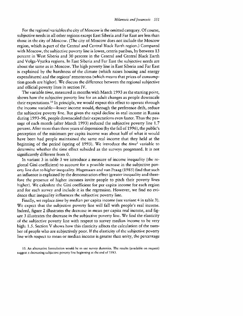
Milanovic and Jovanovic 551
For the regional variables the city of Moscow is the omitted category. Of course,subjective needs in all other regions except East Siberia and Far East are less thanthose in the city of Moscow. (The city of Moscow does not include the Moscowregion, which is.part of the Central and Central Black Earth region.) Comparedwith Moscow, the subjective poverty line is lower, ceteris paribus, by between 13percent in West Siberia and 30 percent in the Central and Central Black Earthand Volga-Vyatka regions. In East Siberia and Far East the subjective needs areabout the same as in Moscow. The high poverty line in East Siberia and Far Eastis explained by the harshness of the climate (which raises housing and energyexpenditures) and the regions' remoteness (which means that prices of consump-tion goods are higher). We discuss the difference between the regional subjectiveand official poverty lines in section IV.
The variable time, measured in months with March 1993 as the starting point,shows how the subjective poverty line for an adult changes as people downscaletheir expectations.10 In principle, we would expect this effect to operate throughthe income variable-lower income would, through the preference drift, reducethe subjective poverty line. But given the rapid decline in real income in Russiaduring 1993-96, people downscaled their expectations even faster. Thus the pas-sage of each month (after March 1993) reduced the subjective poverty line 1.7percent. After more than three years of depression (by the fall of 1996), the public'sperception of the minimum per capita income was about half of what it wouldhave been had people maintained the same real income that they held at thebeginning of the period (spring of 1993). We introduce the time2 variable todetermine whether the time effect subsided as the surveys progressed. It is notsignificantly different from 0.
In variant 3 in table 3 we introduce a measure of income inequality (the re-gional Gini coefficient) to account for a possible increase in the subjective pov-erty line due to higher inequality. Hagenaars and van Praag (1985) find that suchan influence is explained by the demonstration effect (greater inequality and there-fore the presence of higher incomes invite people to pitch their poverty lineshigher). We calculate the Gini coefficient for per capita income for each regionand for each survey and include it in the regression. However, we find no evi-dence that inequality influences the subjective poverty line.
Finally, we replace time by median per capita income (see variant 4 in table 3).We expect that the subjective poverty line will fall with people's real income.Indeed, figure 2 illustrates the decrease in mean per capita real income, and fig-ure 3 illustrates the decrease in the subjective poverty line. We find the elasticityof the subjective poverty line with respect to survey median income to be veryhigh: 1.5. Section V shows how this elasticity affects the calculation of the num-ber of people who are subjectively poor. If the elasticity of the subjective povertyline with respect to mean or median income is greater than unity, the percentage
10. An alternative formulation would be to use survey dummies. The results (available on request)suggest a decreasing subjective poverty line beginning at the end of 1993.

552 THE WORLD BANK ECONOMIC REVIEW, VOL. 13, NO. 3
of people who feel poor will tend to decrease as income goes down. Paradoxi-cally, (subjective) poverty would become less widespread as people's (objective)circumstances deteriorate.
The other coefficients in variant 4 in table 3 are stable, with one exception.The inequality variable (the regional Gini) increases, but is still not significant atthe 5 percent level.
IV. COMPARING REGIONAL SUBJECTIVE AND OFFICIAL POVERTY LINES
We have already seen that the subjective poverty line for an adult is severaltimes higher than the official poverty line (prozhitochnyi minimum) for an adult,although the gap between the two diminishes over time. Here we look at differ-ences in the structure (rankings) of the regional official and subjective povertylines. Table 4 shows the ruble amounts for the official and subjective regionalpoverty lines in 1996. As we would expect, subjective poverty lines are alwayshigher, but the-extent of the gap differs among regions: the official poverty line isless than half of the subjective line in North Caucasus, but is almost two-thirds ofthe subjective line in the North.
The regional differences imply that the official poverty lines do not accuratelyreflect the population's perception of the differences in subjective needs amongthe regions, even though the correlation coefficient between the official and sub-jective poverty lines is 0.85. Figure 5 shows that if the subjective and officialpoverty lines for the city of Moscow are set at 100, the relative subjective povertylines for all but one region (North) are higher than official lines. This findingsuggests a pro-Moscow bias in setting official poverty lines. For example, theofficial poverty line for an adult in the Caucasus is 40 percent lower than that foran adult in Moscow; but the public perception is that it should be only 20 per-cent less (figure 5).
Table 4. Official and Subjective Regional Poverty Lines, 1996(thousands of March 1993 rubles)
Ratio of officialOfficial poverty Subjective to subjective
Region line poverty line poverty line
North 8.30 12.7 0.65Central and Central Black Earth 6.55 11.3 0.58North Caucasus 6.17 12.9 0.48Volga-Vyatka 6.82 11.5 0.59Volga 6.84 12.4 0.55Urals 7.47 13.4 0.56West Siberia 8.79 14.1 0.62East Siberia and Far East 9.06 16.8 0.54Moscow 10.30 16.3 0.63
Note: The subjective poverty lines cover the period January-September 1996.Source: Authors' calculations. Official poverty lines calculated from Goskomstat Rossii (1998, tables
2.7 and 4.20). Subjective poverty lines calculated from regression 2 (table 3).

Milanovic and Jovanovic 553
Figure 5. Official and Subjective Regional Poverty Lines Indexed to Moscow, 1996(Moscow = 100)
Index120
100
80
60
40
20
Moscow East West Urals Caucasus North Volga Volga- CentralSiberia Siberia Vyatka and Central
Black Earth* Official C Subjective
Source: Authors' calculations.
V. How MANY PEOPLE ARE POOR?
In this section we look at the proportion of people who are poor, definedaccording to three criteria. The first criterion labels "subjectively poor" thosehouseholds that assess themselves as poor, that is, households whose view of theminimum income for an adult is greater than their actual adult equivalent in-come (AMYf > Yf* for a given family). A problem with this criterion is that twoidentical households with the same income may be classified as poor and nonpoor,depending on how they perceive their own well-being.
For the second criterion, the "socially subjectively poor," we impose a socialequivalence scale (0 = 0.62) that may not correspond to a household's own equiva-lence scale. This criterion defines as poor those households whose current incomeper equivalent adult (Yfr using 0 = 0.62) is less than the social subjective minimumincome (per adult) for such a household. Regression 3 (the variant with Huber-robust variances and excluding Hadi outliers) predicts this income measure.
According to the third criterion, the poor are those whose current income perequivalent adult (Yf using 0 = 0.62) is less than the official all-Russia poverty line(per working adult).

554 THE WORLD BANK ECONOMIC REVIEW, VOL. 13, NO. 3
Figure 6 shows the share of individuals who are poor according to the threecriteria. We can draw several conclusions. First, an extremely high percentage ofthe population (almost always greater than 60 percent) is subjectively poor, what-ever (subjective) criterion is used. This percentage is consistently higher than thepercentage judged to be poor by the official poverty line.
Second, there is a clear tendency for the subjective poverty headcounts to de-crease with time. The subjective poverty line fell faster than real income, so thatfewer people assessed themselves as poor. The percentage of the socially subjec-tive poor dropped from 90 percent in March 1993 to less than 60 percent inSeptember 1996. At the same time, real average per capita income decreased14 percent.
Third, because real income fell while the official poverty line remained thesame, the proportion of people whose income was less than the official pov-erty line increased from a third of the population in 1993 to more than half in1995, before dropping to near 40 percent in late 1996.11 Thus the decrease inreal income has made more people poor according to an objective and fixedyardstick. Ironically, the same reduction in real income has reduced people'sperception of the minimum income they need to survive and has made fewer ofthem feel poor. Figure 7 shows that the decrease in the percentage of self-assessed poor coincided with the decline in real income. The decline in thepercentage of self-assessed poor decelerated only between mid-1994 and mid-1995, when current real income took another sharp dip: a larger than usualdecrease in real income was required to keep the percentage of the self-assessed poor constant. Thus there are two circumstances under which fewerpeople feel poor: when their real incomes grow quickly or when their realincomes fall (equally) quickly. In Russia, unfortunately, it was the second al-ternative that occurred.
Fourth, in all but two surveys the social subjective poverty line yields higherpoverty headcounts than do people's own assessments (figure 6). This means thatsome households that are socially considered poor do not view themselves assuch.'2 These households fall in the triangle OAB in figure 1, to the left of thesocial poverty line AB. These households' assessment of their well-being is betterthan the "social" assessment, possibly indicating the presence of the much-discussed pockets of social resilience and patience often associated with the Rus-slan population.
11. We cannot compare this figure with the percentage of poor from the official Goskomstat statistics,which ranged between 22 and 31 percent over the same period (Goskomstat Rossii 1998: 79), or thepercentage obtained from the Russian Longitudinal Monitoring Survey (see World Bank 1998: 5). Incomein these surveys is defined to include noncash sources, while in the VCIOM income includes only cashsources.
12. A caveat is in order here. Since we assume that all households have the social equivalence scalereflected in 0 = 0.62, some households that classify themselves as poor may in fact have a lower 0 and thusnot regard themselves as poor. The opposite classification mistake is possible for nonpoor householdswhose 0 is greater than 0.62.

Milanovic and Jovanovic 555
Figure 6. Share of Poor Individuals in the Total Population According to ThreeConcepts of Poverty, 1993-96
Percentage poor
100
90 According to societ>
80 -
70-According to their owvn viewve
60 -
50-50 - ~~According to the
40 -official poverty line-
30 -
20 I I l l
0 5 10 15 20 25 30 35 40Month (March 1993=1)
1993 1994 1995 1996
Note: All shares are individual-basedSource- Authors' calculations.
VI. CONCLUSIONS
In the three and a half years (March 1993 to September 1996) covered by theVCIOM surveys of the Russian population, real per capita income fell 15-20 per-cent. This decrease came on top of severe income contractions in 1991 and 1992.Thus the Russian population experienced one of the worst peacetime depressionsin the twentieth century. At the same time, income inequality increased substan-tially. In this article we have analyzed what happened to the public's perceptionof the minimum income needed to make ends meet under these exceptionalconditions.
We would expect the subjective poverty line to decrease as well. Indeed, theelasticity of the subjective poverty line with respect to median population incomeis above unity-a very high 1.5. The time variable is significant, as the subjectivepoverty line fell 1.7 percent each month. Thus after more than three years ofdepression, the public's perception of the minimum income an adult would needto survive was about half of what it would have been had real incomes remainedwhat they were at the beginning of the period.
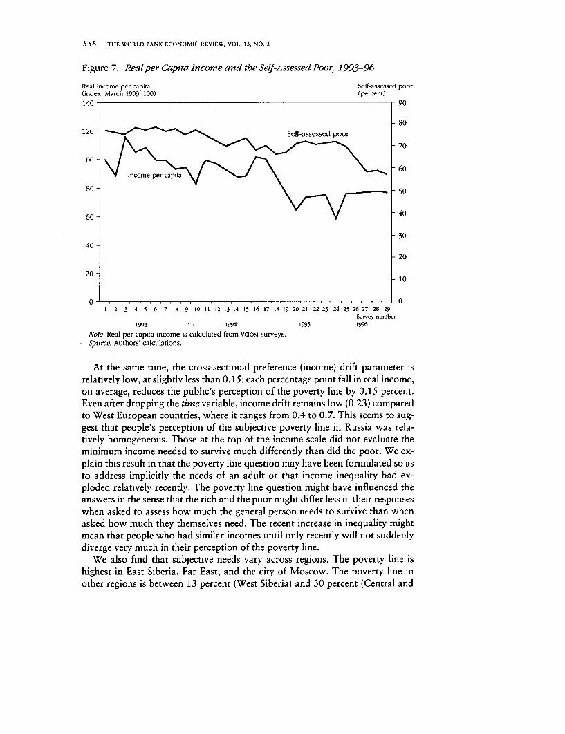
556 THE WORLD BANK ECONOMIC REVIEW, VOL. 13, NO. 3
Figure 7. Real per Capita Income and the Self-Assessed Poor, 1993-96
Real income per capita Self-assessed poor(index, March 1993-100) (percent)
140- 90
-80
120 8
-70
100 -60
80 V tnncome per6c
80 -50
60- - 40
3040 -
-20
20-10
0 - 01 2 3 4 5 6 7 8 9 10 11 12 13 14 15 16 17 18 19 20 21 22 23 24 25 26 27 28 29
Survey number
1993 1994' 1995 1996
Note Real per capita income is calculated from VcIOM surveys.
Source: Authors' calculations.
At the same time, the cross-sectional preference (income) drift parameter isrelatively low, at slightly less than 0.15: each percentage point fall in real income,on average, reduces the public's perception of the poverty line by 0.15 percent.Even after dropping the time variable, income drift remains low (0.23) comparedto West European countries, where it ranges from 0.4 to 0.7. This seems to sug-gest that people's perception of the subjective poverty line in Russia was rela-tively homogeneous. Those at the top of the income scale did not evaluate theminimum income needed to survive much differently than did the poor. We ex-plain this result in that the poverty line question may have been formulated so asto address implicitly the needs of an adult or that income inequality had ex-ploded relatively recently. The poverty line question might have influenced theanswers in the sense that the rich and the poor might differ less in their responseswhen asked to assess how much the general person needs to survive than whenasked how much they themselves need. The recent increase in inequality mightmean that people who had similar incomes until only recently will not suddenlydiverge very much in their perception of the poverty line.
We also find that subjective needs vary across regions. The poverty line ishighest in East Siberia, Far East, and the city of Moscow. The poverty line inother regions is between 13 percent (West Siberia) and 30 percent (Central and

Milanovic and Jovanovic S57
Central Black Earth, and Volga-Vyatka) less than that in the city of Moscow.These differences are smaller than the differences in the official regional povertylines, suggesting the existence of a pro-Moscow bias in setting the official lines.
During the time period studied, a very high percentage of the population (al-ways more than 60 percent) considered itself poor according to the social subjec-tive poverty line. The percentage of the subjectively poor tended to decline morethan proportionately with the decline in real income. We thus face a somewhatunusual situation in that the percentage of the subjectively poor decreased moreor less in step with the reduction in people's real income. Only larger than usualdeclines in income kept the percentage of the poor unchanged.
It is also noteworthy that the percentage of the self-assessed poor was alwayslower than the percentage of the socially subjective poor. Thus part of the popu-lation regarded their own income as adequate, although they were deemed pooraccording to the public's perception of minimum income. These last two find-ings-the decline in the percentage of the subjectively poor as real income felland the lower percentage of self-assessed poor than socially subjective poor-suggest that to adapt to the worsening circumstances, people sharply reducedtheir perception of the minimum income needed for survival.
APPENDIX A. CONSTRUCTION OF THE INCOME VARIABLES
The VCIOM data set contains several income variables that are measured onboth the individual and household levels. Two reported income variables areindividual main income and individual income from a second job. Household(family) income components include family income from a main job, family in-come from a second job, income from private sector activities, pensions, othersocial transfers, stipends, alimony, income from financial assets (stocks, bonds,vouchers, interest income), income from sale of self-produced goods, and othermonetary income.
The total family income variable is also included in the data set, and it issupposed to equal the sum of the family income components, but rarely does. Insome cases total family income was reported missing, although the income com-ponents were available. Also, in some cases, even though all the income compo-nents were missing, total family income took a positive value. Furthermore, therewere inconsistencies in reported individual and family main income, as well asbetween individual and family income from a second job.
We computed total family income as the sum of the family income compo-nents, that is, as the sum of main job income, income from a second job, andincome from private sector activities, pensions, benefits and subsidies, stipends,alimony, income from financial assets, income from sale of self-produced goods,and other monetary income. This was done as follows:
* The individual main income variable before April 1994 corresponds to thevariable main_inc, and to the variable main_in2 thereafter (the two variables

558 THE WORLD BANK ECONOMIC REVIEW, VOL 13, NO 3
have the same definition, only the name has been changed). Thus for anysurvey after April 1994, we replace the value of main_inc with main_in2.However, no data are available for November 1995 because that survey didnot ask a question concerning the main income; therefore we do not haveobservations on the main individual income for that survey.The variables family income from a main job and from a second job are atleast equal to the corresponding variables for the individual. Therefore, wherethe data on family income are missing or less than the individual income,we replace the value of family income with the observation on individualincome.
In cases where all the income components are missing, we replace our totalincome with vcLoM-computed total income. Also, where our total income is lessthan the vcioM-computed total income, we take the VCIOM value. Although thecode book reports that a value of zero should be treated as a missing variable,both true zero and missing responses seem to be coded as zero. We do not at-tempt to distinguish between the two because efforts in that direction are un-likely to be fruitful.
APPENDIX B. THE HADI PROCEDURE
The basic outline of the Hadi (1992, 1994) procedure is as follows. We definea measure of distance from an observation to a set (cluster) of points. The pointsare scatter plots, with one variable on the x-axis and one on the y-axis. Initially,we have only three points because we operate with only two variables (we as-sume explicitly that outliers are in the income variables and not in human capitalor other categorical variables). We introduce an additional point (observation oftotal income and pov_line) and measure the distance between that point and theinitial group of points. Once the base cluster is established, a more standardmean-based center of the r-observations cluster is defined, and the r + 1 observa-tions closest in the covariance-matrix sense are chosen as a new base cluster. Thisis repeated until the base cluster has a certain number of points, and when itreaches the critical size, the distance rule changes. A base cluster of r points isselected (r is defined as k + 1, where k is the number of variables), and then thatcluster is continually redefined by taking the r + 1 point "closest" to the cluster asthe new base cluster. The distance rule used in the STATA hadimvo procedure isbased on a matrix of second moments, with the median of variables removed). Inthis article we use variables tot (total income) and pov_line to flag the Hadioutlier.
REFERENCES
The word "processed" describes informally reproduced works that may not be com-monly available through library systems.

Milanovic and Jovanovic 559
Atkinson, Anthony B., Lee Rainwater, and Timothy M. Smeeding. 1995. Income Distri-bution in OECD Countries: Evidence from the Luxembourg Income Study. OECD SocialPolicy Studies 18. Paris: Organisation for Economic Co-operation and Development.
Braithwaite, Jeanine. 1997. "The Old and the New Poor in Russia." In Jeni Klugman,ed., Poverty in Russia. Washington, D.C.: World Bank.
Flik, Robert J., and Bernard M. S. van Praag. 1991 "Subjective Poverty Line Definitions."De Economist 139(3):311-31.
Frijters, Paul, and Bernard M. S. van Praag. 1994. "Estimates of Poverty Ratios andEquivalence Scales for Russia and Parts of the Former USSR." Rotterdam. Processed.
Glinskaya, Elena, and Jeanine Braithwaite. 1998. "Poverty, Inequality, and Income Mo-bility in Russia, 1994-96." Paper prepared for the American Population Association,Chicago, April 2-4. Processed.
Goedhart, Theo, Victor Halberstadt, Arie Kapteyn, and Bernard M. S. van Praag. 1977."The Poverty Line: Concept and Measurement." The Journal of Human Resources12(4): 503-20.
Goskomstat Rossii. 1995. Rossiiski Statisticheskiy Ezhegodnik 1995. Moscow.. 1998. Rossiya v tsifrah 1998. Moscow.
Hadi, A. S. 1992. "Identifying Multiple Outliers in Multivariate Data." Journal of theRoyal Statistical Society, Series B, 54(3):761-71.
.1994. "A Modification of a Method for the Detection of Outliers in MultivariateSamples." Journal of the Royal Statistical Society, Series B, 56(2):393-96.
Hagenaars, Alvi J. M., and Bernard M. S. van Praag. 1985. "A Synthesis of Poverty LineDefinitions." Review of Income and Wealth 31(2):139-54.
Kahneman, Daniel, and Richard Thaler. 1991. "Economic Analysis and the Psychologyof Utility: Applications to Compensation Policy." American Economic Review Papersand Proceedings 81(2):341-46.
Lokshin, Michael, and Barry M. Popkin. 1999. "The Emerging Underclass in the RussianFederation: Income Dynamics, 1992-96." Economic Development and Cultural Change47(4):803-29.
Milanovic, Branko. 1998. Income, Inequality, and Poverty during the Transition fromPlanned to Market Economy. Washington, D.C.: World Bank.
Ovcharova, Liliana, E. Turuntsev, and Irena Korchagina. 1998. "Bednost': gde porog."Voprosi ekonomiki 7(2):61-73.
Ravallion, Martin, and Michael Lokshin. 1999. "Subjective Economic Welfare." PolicyResearch Working Paper 2106. World Bank, Washington, D.C. Processed.
van Praag, Bernard M. S. 1971. "The Individual Welfare Function in Belgium: An Em-pirical Investigation." European Economic Review 2(3):227-69.
van Praag, Bernard M. S., and Robert J. Flik. 1992. "Subjective Poverty." Final report inthe framework of the European Eurostat Project, Enhancement of Family Budget Sur-veys to Derive Statistical Data on Least Privileged Groups. Foundation for EconomicResearch and Research Institute for Population Economics, Rotterdam. Processed.
van Praag, Bernard M. S., and Nico Van der Saar. 1988. "Empirical Uses of SubjectiveMeasures of Well-Being: Household Cost Functions and Equivalence Scales." Journalof Human Resources 23(2):193-210.
World Bank. 1998. "Poverty Policy in Russia: Targeting and the Longer-Term Poor."Eastern Europe and Central Asia Region. Poverty Reduction and Economic Manage-ment (PREM), Washington, D.C. Processed.

THE WORLD BANK ECONOMIC REVIEW, VOL. 13, NO. 3: 561-78
Labor Market Analysis and Public Policy:The Case of Morocco
Julia Lane, Guillermo Hakim, and Javier Miranda
This article uses detailed industry and household data to understand why Morocco'slabor market performed poorly in 1985-95. The data indicate that marked structuralchanges and weak demand in the product market were responsible. This article makestwo contributions to the literature. The first is specific: it underscores that the demandfor labor is a derived demand and that the performance of the product market is animportant determinant of the performance of the labor market. The second is moregeneral: it demonstrates that this kind of microeconomic analysis, using data sets thatare often available in developing countries, can inform policy design.
Since 1985 Morocco has experienced increasing unemployment in urban areasand stagnant wages in the manufacturing sector (World Bank 1995). We mustunderstand the reasons for the labor market's poor performance in order to de-sign policies that will help to generate adequate jobs and earnings. In this articlewe use two data sets for Morocco to demonstrate how standard econometrictechniques can disentangle the causes of such poor performance. These types ofdata sets are often available in developing countries.
We look at demand- and supply-side factors to explain Morocco's stagnantearnings growth. On the supply side, this stagnation could reflect a deteriorationin the quality of the labor force. If so, policy reform should concentrate on im-proving the external and internal efficiency of expenditures on general educationand vocational training. On the demand side, weak job and earnings growth maybe a result of inappropriate government intervention: a stringent labor code thatimpedes firms' ability to hire and fire workers or a minimum wage policy thatreduces firms' incentives to create jobs. If so, policy reform should include legis-lation to liberalize labor market regulations.
In this article we argue that the labor market's poor performance during 1986-95 can be traced to, first, a shift in the employment composition of manufactur-ing to low-paying industries linked to the export sector, which depressed averagewages, and, second, stagnant product demand, which weakened the derived de-mand for labor. Stagnant product demand also explains Morocco's high unem-
Julia Lane is with the Urban Institute, Guillermo Hakim is with the Human Development Group of theMiddle East and North Africa Region at the World Bank, and Javier Miranda is with the Department ofEconomics at American University. Their e-mail addresses are [email protected], [email protected],and [email protected].
( 1999 The International Bank for Reconstruction and Development/THE WORLD BANK
561
562 THE WORLD BANK ECONOMIC REVIEW, VOL. 13, NO. 3
ployment: although there has been some employment growth in the formal manu-facturing sector, that growth has been too weak to offset the expansion of theurban labor force.
Supply-side changes over the past decade have put upward, not downward,pressure on earnings. A much higher proportion of workers were in their primeearning years in 1993 than in 1986. The average education level of the laborforce was also higher in 1993 than in 1986. As for demand, standard measures oflabor market flexibility show that labor market rigidity is not the prime reasonfor poor performance: Morocco's recourse to temporary contracts has allowedfirms to adjust their employment levels as freely as firms in countries that arepart of the Organisation for Economic Co-operation and Development (OECD).
In particular, the elasticity of labor demand with respect to output, rates of jobcreation and destruction, and speed of adjustment to demand shocks in Moroccoare similar to those in other OECD countries.
One reason for the stagnant wages in Morocco is that low-paying industrieshave been the major source of employment growth. The three industries with thefastest employment growth over the past decade-processed food, textiles, andclothing-are also the three with the lowest average earnings per worker. Anobvious policy measure for stimulating the labor market would be one that seeksto increase sales as well as the earnings and productivity of workers in suchfirms. Although the average performance of firms has been weak (in terms ofgenerating revenue, value added, or sales), key industries, such as textiles andclothing, have outperformed other industries, with clothing increasing its em-ployment more than 300 percent over the decade.
I. DATA
We use two data sets in the analysis. Data describing the supply side comefrom the World Bank's 1990-91 Moroccan Living Standards Measurement Sur-vey (LSMS). This household survey provides detailed socioeconomic informationon about 19,000 individuals. Of these, 9,685 are between the ages of 18 and 65,and 1,946 report wage and salary earnings (40 percent of men and 8 percent ofwomen). This last group is the basis of our analysis.
The fact that the analysis focuses on a subset of the working population high-lights an important point: because of the difficulty of collecting data on the infor-mal sector, our analysis applies only to the formal sector. Although this limita-tion makes the results less general, stimulating the growth of the formal sector isa key policy focus of both the Moroccan government and the World Bank. In-deed, a healthy formal sector is critical to economic development.
Most of the key variables used are standard for this type of study-age, educa-tion, industry and occupation, and region of residence. However, the earningsmeasure is monthly earnings, which does not include benefits, such as pensions,holidays, and in-kind transfers. We measure education in years according to thelevel of qualification achieved. Since the survey does not capture actual experi-

Lane, Hakim, and Miranda 563
ence, we construct a measure of potential experience as the age of the workerminus years of education minus seven.
Data on the demand side come from an annual (1984-95) census of all manu-facturing firms in the formal sector with more than 10 workers and a sample ofthose with 10 or fewer. There are a total of 61,897 observations (starting with3,692 firms in 1984 and ending with 6,036 firms in 1995), dropping firms thatreport having no employees. Of the full sample of firms, 59,398 report in threeor more years. But the usual problems with nonreporting arise: only 51,858 ob-servations have value added measures, for example. There is also the possibilitythat firms spuriously drop into and out of the data set. But since more than 68percent of the firms report positive employment in at least 9 of the 12 years, andthese firms account for 80 percent of employment, the qualitative impact on thedata is minimal.
Although the key variables we use are standard, it is worth discussing themeasurement of some of them. Firms report both permanent employment andtotal days worked by temporary employees. We transform this measure into to-tal employment by summing permanent employment and the annual equivalentof temporary employment (total days worked divided by 220). We calculate av-erage wages by dividing total payroll by total employment-so lower wages mayreflect either a change in the composition of workers or a true decrease in wagesfor a particular type of worker.
The measure of capital stock is difficult to construct, and we follow the litera-ture in using the gross book value of fixed assets, which is reported in 1990, andthe perpetual inventory method of depreciating investment, which is reportedevery year. There are obvious problems with this approach. First, and most criti-cal, the key base variable-book value-does not represent the economic valueof capital. Second, firms do not report the proportion of their capital that is plantand the proportion that is equipment. Third, many firms do not report the bookvalue at all. Finally, the estimate of the depreciation rate (chosen to be 5 percent)is arbitrary and does not reflect industry differences or different proportions ofplant and equipment. We thus follow Currie and Harrison (1997) and use avariation of firm fixed effects to verify the robustness of the results when capitalstock is used.
II. WAGES AND EMPLOYMENT rN MOROCCO
Data from the annual employment survey conducted by the government'sStatistical Institute show that in the past decade Morocco's population growthhas averaged 2.2 percent a year, and its labor force growth has been slightlylower. But the growth rate of the urban labor force has been much higher be-cause of strong migration from rural areas to the cities. Between 1986 and1995 the urban labor force grew at 5 percent a year, while the rural labor forcedeclined in absolute terms. However, net job growth in urban areas was only 4percent a year. This differential, coupled with increasing participation rates by

564 THE WORLD BANK ECONOMIC REVIEW, VOL. 13, NO. 3
women, boosted unemployment rates and shifted jobs to the informal sector.The official urban unemployment rate hovers around 20 percent, affecting about1.2 million people.
Between 1985 and 1995 employment growth in the formal urban sector wasstrongly correlated with the performance of manufactured exports. Employmentgrew with manufactured exports in the late 1980s, but slowed considerably inthe 1990s (figure 1).
The period of growth in the 1980s was the result of several factors. First,Morocco benefited from its privileged access to European markets, which it se-cured through various trade agreements with the European Union. Second, manu-factured exports became more competitive when the real effective exchange ratedepreciated because of falling unit labor costs (measured in local currency). Dur-ing the 1980s manufactured exports grew at an annual rate of 23 percent, andemployment grew at 11 percent. Although this combination of factors producedstrong employment expansion, it was short-lived.
In the 1990s unit labor costs reversed their downward trend as real wages roseslightly and productivity declined (figures 1 and 2). At the same time, the realeffective exchange rate appreciated, making Moroccan exports more expensiveabroad. All of these elements came together at a moment when Eastern Europeanand Asian competitors were also granted access to European markets, pushingout Moroccan goods. Manufactured exports grew at only 4 percent a year dur-ing 1990-95, and employment grew at less than 2 percent a year.
Figure 1. Indicators of Manufacturing Performance, 1985-95
Indexed to 1990 level
120 -
veage earnings >
100
80 -
Total employment
60 -
1985 1990 1995
Source: Authors' calculations.

Lane, Hakim, and Miranda 565
Figure 2. Indicators in Firm Performance, 1985-95
110 -Average productivity
100
0
C\
90 -Average revenueL
80-
70 l-l_l
1985 1990 1995
III. CONCEPTUAL FRAMEWORK
Our formal analysis follows a simple supply and demand approach of the typeproposed by Bound and Johnson (1992). The aggregate manufacturing workforceis composed of i demographic groups defined by age and education, working in jdifferent industries. The wage rate of each group of workers is Wi, and the rela-tive rent of each worker in industry j is gi. The average wage in manufacturing attime t, wt, is a simple weighted average of the number of workers in each skillgroup (pit ) at time t and their relative rents:
(1) Wt = £, £j (Pi, W, + p,t pj).
Wage changes in this model can be written as
(2) Wt- W-i = Z, [(Wit - W l) Pi, + W,, (P,, - Pil-l)]
+ X, [(.t - .,y) Pit + R,t- (P,t - Pi t-)-
If we assume that the wage of each demographic group is exogenous and not afunction of the group's relative supply, then wage changes are simply driveneither by changes in the number of workers in each demographic group or by theallocation of the same group of workers across different industries. This is clearlya very strong assumption, since it reduces the importance of wages as a mecha-nism for allocating resources. However, since neither linked worker-firm datanor repeated, relatively large-scale household surveys exist, we are forced to fo-cus on quantity rather than price adjustments.

566 THE WORLD BANK ECONOMIC REVIEW, VOL. 13, NO. 3
In the next two sections we apply this model to examine explanations thatfocus on changes in the relative supply of different groups of labor and those thatfocus on shifts in product demand.
IV. LABOR SUPPLY
Earnings may become stagnant because of a deterioration in the quality of thelabor force. It may be that the average educational level has deteriorated or thatthe workforce has fewer experienced prime-age workers. In this section we ex-amine each of these possibilities by simulating how a shift in the composition ofthe labor force would have affected average earnings had wages remained con-stant during 1986-95.
The Distribution of Education in the Urban Labor Force
The effect that the distribution of education will have on average earningsdepends on the return to education and the distribution of workers with differenttypes of education. We estimate returns to education with standard Mincerianearnings models using LSMS data and examine the distribution of workers usingpublished national statistics.
In most countries age-earnings profiles vary with the level of education: work-ers with relatively little education have flatter earnings profiles than workerswho are highly educated. This pattern holds in Morocco. The results of ourMincerian regressions indicate that the return to investment in education is about10 percent a year, using hourly earnings as the dependent variable (table 1). Atleast part of this return comes from an economic rent associated with working incertain industries and occupations. Once industry and occupational dummies areincluded in the regression, the return to education drops to about 4-5 percent.
Given that the return to education is positive and reasonably large, we thenask whether stagnant real earnings result from a deterioration in the quality ofthe labor force. In general, this is unlikely, since the education level of the poten-tial labor force does not change rapidly over time. However, the education levelof the employed labor force may vary markedly if workers at one end of theeducation spectrum drop out or if large cohorts of uneducated workers enter. InMorocco the change has been an increase in the quality of labor: the proportionof workers with no primary school qualifications fell between 1986 and 1990and again, more sharply, between 1990 and 1993.
Thus the net effect of the changing educational structure of the employed laborforce was to raise earnings over what they would have been otherwise. In particu-lar, because of the increase in the education level of the employed labor force dur-ing 1986-93, average earnings actually rose by DH240 (dirhan) relative to whatthey would have been had education remained at the 1990 level. These resultssuggest that the immediate source of stagnant earnings and productivity growthwas not a deterioration in the educational quality of the employed formal laborforce. The proportion of highly educated workers rose. And since the wages of
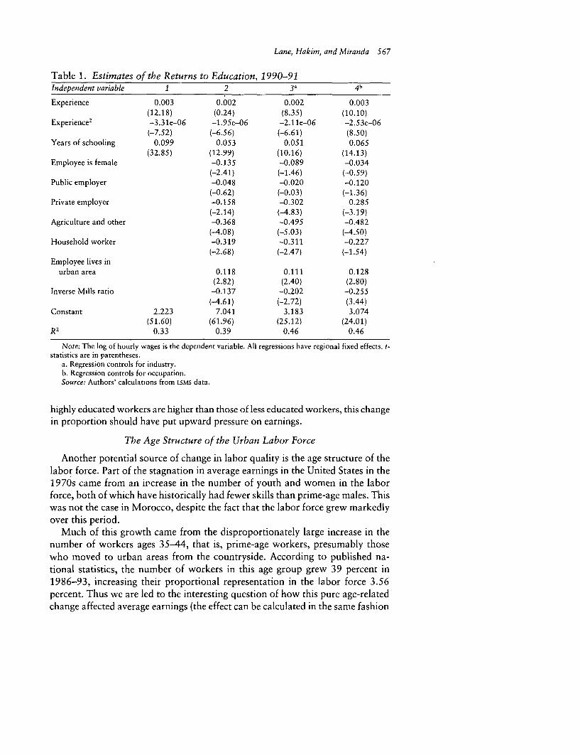
Lane, Hakim, and Miranda 567
Table 1. Estimates of the Returns to Education, 1990-91Independent variable 1 2 3a 4h
Experience 0.003 0.002 0.002 0.003(12.18) (0.24) (8.35) (10.10)
Experience 2 -3.3 le-06 -1.95e-06 -2.11 e-06 -2.53e-06(-7.52) (-6.56) (-6.61) (8.50)
Years of schooling 0.099 0.053 0.051 0.065(32.85) (12.99) (10.16) (14.13)
Employee is female -0.135 -0.089 -0.034(-2.41) (-1.46) (-0.59)
Public employer -0.048 -0.020 -0.120(-0.62) (-0.03) (-1.36)
Private employer -0.158 -0.302 0.285(-2.14) (-4.83) (-3.19)
Agriculture and other -0.368 -0.495 -0.482(-4.08) (-5.03) (-4.50)
Household worker -0.319 -0.311 -0.227(-2.68) (-2.47) (-1.54)
Employee lives inurban area 0.118 0.111 0.128
(2.82) (2.40) (2.80)Inverse Mills ratio -0.137 -0.202 -0.255
(-4.61) (-2.72) (3.44)Constant 2.223 7.041 3.183 3.074
(51.60) (61.96) (25.12) (24.01)R2 0.33 0.39 0.46 0.46
Note. The log of hourly wages is the dependent variable. All regressions have regional fixed effects. t-statistics are in parentheses.
a. Regression controls for industry.b. Regression controls for occupation.Source: Authors' calculations from LSMS data.
highly educated workers are higher than those of less educated workers, this changein proportion should have put upward pressure on earnings.
The Age Structure of the Urban Labor Force
Another potential source of change in labor quality is the age structure of thelabor force. Part of the stagnation in average earnings in the United States in the1970s came from an iPcrease in the number of youth and women in the laborforce, both of which have historically had fewer skills than prime-age males. Thiswas not the case in Morocco, despite the fact that the labor force grew markedlyover this period.
Much of this growth came from the disproportionately large increase in thenumber of workers ages 35-44, that is, prime-age workers, presumably thosewho moved to urban areas from the countryside. According to published na-tional statistics, the number of workers in this age group grew 39 percent in1986-93, increasing their proportional representation in the labor force 3.56percent. Thus we are led to the interesting question of how this pure age-relatedchange affected average earnings (the effect can be calculated in the same fashion

568 THE WORLD BANK ECONOMIC REVIEW, VOL. 13, NO. 3
as above). The change-in the age distribution actually increased mean earnings inMorocco by DH52 in excess of what they would have been had the age distribu-tion remained the same.
In sum, then, changes in the age and education composition of the workforceraised the level of earnings and should have increased labor productivity in urbanareas. Other explanations for the stagnation must be found.
V. LABOR DEMAND
Since stagnant average earnings are clearly not the result of changes in laborsupply, we turn to the demand side of the market for an explanation. Earningscould stagnate if the demand for labor does not respond normally to demandshocks, if the labor market is unable to reallocate workers from less productiveto more productive activities, or if there has been a structural shift in employ-ment from high-paying to low-paying industries. We examine each of these inturn.
The Derived Demand for Labor
Since the demand for labor is a derived demand, it is extremely important toexamine the health of the product market. In Morocco average firm performancedid not change markedly over 1985-95 (figure 2). Revenue generated per workeractually fell below the 1985 level, as did productivity. It is worth noting in thiscontext that although exports per worker grew dramatically in the late 1980s,the 1990s have seen a substantial drop in the growth rate, with investment actu-ally falling in 1994 and 1995.
We can examine the effect of this change on labor demand by estimating fairlystandard labor demand equations of the form:
(3) In Lft = 0 + lrn wft + 2 In VAf, +03 t +eft.
Thus the demand for labor, L, in firm f at time t is determined by the averagewage of the workers, w; and the value added, VA, in firm f at time t. We face twoestimation problems. First, the Moroccan data are very similar to U.S. data, whichare characterized by vast heterogeneity across firms because of differences in thequality of inputs, outputs, and managers (Dunne and Roberts 1993; Haltiwanger,Lane, and Spletzer 1999). Fortunately, however, our data set is quite rich: itcomprises longitudinal data spanning 12 years and about 5,000 firms. Thus weare able to follow Dunne and Roberts (1993) in using fixed effects both to ac-count for unobservable heterogeneity and to minimize simultaneity bias. Thesecond problem is that both wages and value added are likely to be contempora-neously correlated with the error term. We address this issue by also reportingthe results using lagged values as instruments.
The first column in table 2 reports the results of estimating equation 3 byordinary least squares (controlling for fixed effects). The elasticity of labor de-mand with respect to value added is 0.368, indicating that employment is indeed

Lane, Hakim, and Miranda 569
Table 2. Determinants of Manufacturing Labor Demand, 1985-95Ordinary least Instrumental
Independent variable squares variables
Value added 0.368 0.181(74.80) (37.70)
Average wage -0.482 -0.143(59.07) (18.98)
Year 0.036 0.013(46.51) (14.91)
Constant -1.209 1.14(18.22) (14.15)
R2 0.95 0.93Number of observations 62,179 55,990Number of firms 8,161 7,531
Note: t-statistics in parentheses.Source: Authors' calculations.
responsive to product demand shocks. Both this elasticity and the own-wageelasticity are well within the range of empirical estimates for other countries(Hamermesh 1993), regardless of whether we use the least squares estimates orthe instrumental variable estimates. Hence firms in Morocco respond to marketstimuli in similar ways as firms in other countries. However, the growth rate ofemployment in each firm is extremely sluggish: firms expand about 1 percent ayear.
The results are stable when we examine firms at a more detailed level (table 3).The own-wage elasticity always falls within reasonable bounds and, in fact, isremarkably stable for firms of different sizes. Export-oriented firms (defined asfirms whose sales are more than 50 percent exports) are more responsive to wageincreases than are their domestically oriented counterparts. State-owned firms(defined as firms with more than 50 percent state ownership) are more wagesensitive than private firms.
These results suggest that Moroccan labor demand is not much different fromthat in other countries, at least with respect to observable responses to marketstimuli. It may be true that regulation lowers labor demand in all countries, butthe evidence does not suggest that the effect in Morocco is unusually strong. Wenow examine labor market flexibility by comparing job creation and job destruc-tion rates in Moroccan firms.
Labor Flexibility
Foster, Haltiwanger, and Krizan (1998) establish that in the United Statesmore than half of productivity growth is due to the reallocation of resourcesfrom less productive to more productive firms. Thus the movement of workersacross firms is likely to be an important source of productivity (and hence wage)growth. In this section we examine the two components of job reallocation: jobcreation (the positive change in employment at the firm level, divided by averagefirm employment) and job destruction (the negative change in employment at the
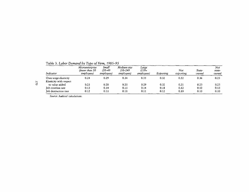
Table 3. Labor Demand by Type of Firm, 1985-95Microenterprise Small Medium-size Large Not(fewer than 20 (20-49 (50-249 (250+ Not State- state-
Indicator employees) employees) employees) employees) Exporting exporting owned owned
Own-wage elasticity 0.24 0.29 0.34 0.35 0.32 0.22 0.36 0.25Elasticity with respect
to value added 0.25 0.20 0.25 0.29 0.32 0.21 0.23 0.23Job creation rate 0.13 0.14 0.15 0.14 0.18 0.12 0.12 0.13Job destruction rate 0.12 0.11 0.11 0.11 0.12 0.10 0.10 0.10
Source: Authors' calculations.

Lane, Hakim, and Miranda 571
firm level, divided by average firm employment), which have often been used asmeasures of labor market flexibility (see Davis, Haltiwanger, and Schuh 1996).Indeed, OECD (1996) finds a negative relationship between the job destructionrate and the index of labor market regulation.
With average job creation and destruction rates hovering around 12 percent,Morocco shows a degree of labor market flexibility similar to that of OECD coun-tries (figure 3). These figures confirm earlier work by Currie and Harrison (1997),who offer anecdotal evidence that labor market adjustment is quite fluid anddemonstrate that another measure of labor market flexibility-firms' speed ofadjustment to demand shocks-falls within international norms.
The difference between the volatility in permanent and temporary employ-ment is also marked, suggesting that Moroccan firms are using temporary em-ployment as a way of adjusting to demand shocks (figures 4 and 5). Using tempo-rary employment in this way, while consistent with employment practices in othercountries, does pose some long-run concerns for the development of a skilled andproductive workforce and for the flexibility of permanent workers.
Again, a closer examination of these trends suggests that all classes of firms,defined by size, export orientation, and state ownership, are roughly equivalentto international standards of flexibility (see the last two rows of table 3). Theresult for state-owned firms is particularly surprising and suggests that there iswidespread avoidance of the labor code, even in the state-owned sector.
Figure 3. Job Creation and Destruction Rates for All ManufacturingEmployment, 1985-95
Percent
20-
Job creation rateA
15-
10-
Job destruction ratc
5-
1985 1990 1995
Source: Authors' calculations.

572 THE WORLD BANK ECONOMIC REVIEW, VOL. 13, NO. 3
Figure 4. Job Creation and Destruction Rates for Permanent Employment,1985-95
14 -
12 -
10
8
1985 1990 1995
Figure 5. Job Creation and Destruction Ratesfor Tmporary Employment,1 985- 95
8 -
Job creation rate6
4
2
job destruction rate
0
1985 1990 1995

Lane, Hakim, and Miranda 573
Sectoral Shifts
The last possible explanation for stagnant wage growth is that the structure ofthe economy has changed from high-productivity and high-wage industries tolow-productivity and low-wage industries. That this is a possibility is immedi-ately evident from an examination of individual industries (table 4). The threelargest industries that also display some of the highest employment growth-processed food, textiles, and clothing-are the three with some of the lowestearnings (they are ranked sixteenth, fourteenth, and eighteenth, respectively, interms of average payroll). Although earnings are much higher in beverages andtobacco, electrical and electronic equipment, and base metal products, job cre-ation in these industries has been relatively flat or declining. The only industry tocombine both high earnings and high employment growth is the chemicals industry.
Another way of looking at sectoral changes is through the job creation anddestruction rates of high-wage and low-wage firms. We call firms "high-wage" iftheir average payroll exceeds the average payroll for all firms in a given a year.We classify "low-wage" firms similarly. We then track their patterns of job cre-ation and job destruction over time (figure 6). It is clear that job creation and jobdestruction are higher in low-wage than in high-wage firms and that net jobcreation is positive for low-wage firms and negative for high-wage firms. In otherwords, employment growth is occurring at the low end of the wage spectrum.
Finally, we decompose the growth in average wages between 1984 and 1995by simplifying equation 2 to focus solely on changes in industry composition,rather than on changes in workforce composition. We thus note that w, = witpit,where w, is the average wage at time t, wi, is the average wage in industry j at timet, and pi, is industry j's employment share. Thus:
(4) w, - w t-l = X, [Pjt(wt - rv,_) + wit-, (Pit - PI,)
or, the change in the average wage is the sum of the change in the wage of eachindustry weighted by that industry's share of employment (the first term on theright side) and the change in the industry's share of employment, weighted byaverage wages at time t - 1 (the second term on the right side). Applying thissimple decomposition reveals that had the sectoral distribution of employmentremained the same between 1984 and 1995, average wages would have been 9.8percent higher. The same holds true for a similar decomposition of productivity:because employment has grown in the least productive sector of the economy, ifemployment shares had stayed the same between 1985 and 1995, average pro-ductivity would have been 20.1 percent higher.
VI. POLICY IMPLICATIONS
Our initial concern was to explain poor employment and earnings growth inthe Moroccan economy. The evidence presented above strongly suggests that thepoor performance in the past 12 years is not a result of inadequate education or

Table 4. Labor Market Indicators by IndustryPercentagegrowth in Percentage
Average average Rank Number of employment Rankearnings earnings (earnings employees growth (employment
Industry (1995) (1 984-95) level) (1995) (1 984-95) growth)Food products 33.15 9.03 9 27,197 26.81 14Processed food products 23.02 28.45 16 60,748 64.41 6Beverages and tobacco 56.64 47.58 1 10,201 2.73 17Textiles and hosiery 25.79 4.76 14 70,213 48.89 10Clothing excluding footwear 16.66 30.10 18 101,771 352.71 1Leather products including shoes 19.03 -8.42 17 15,714 35.19 12Lumber and wood products 24.61 24.94 15 12,850 18.76 16Paper, cardboard, and printing 33.63 3.31 8 16,825 66.24 5Glass, cement, and ceramic products 31.45 13.18 12 33,266 61.53 7Base metal products 49.03 20.95 3 1,932 -33.87 18Metalwork, excluding machinery,
and transport equipment 34.40 10.30 7 23,948 46.5S 11Machinery and equipment 35.79 6.90 6 7,137 27.58 13Transportation equipment 44.30 6.73 5 12,498 122.02 2Electrical and electronic equipment 45.49 17.17 4 10,703 24.57 15Office machines, measuring 29.27 -22.79 13 1,013 55.70 9Chemicals and related products 51.13 10.64 2 31,342 89.96 4Rubber and plastic products 32.87 3.09 10 12,362 55.94 8Miscellaneous manufactures 32.01 36.63 11 651 103.53 3
Source: Authors' calculations.

Lane, Hakim, and Miranda 575
Figure 6. Job Creation and Destruction Rates by Wage Category, 1985-95
Low-Wage Firms High-Wage Firms
Percent Percent20- Job creation rate 20-
15- 15
Job destruction rate
10~ g 10-
0 job destruio rat
5 Job creation rate
1985 1g90 1995 1985 1990 1995Source Authors' calculations
labor market rigidities. Rather, structural changes in Morocco were behind thelabor market's poor performance. If the strong growth of the clothing industry,for example, had been seen in the rest of the manufacturing sector, overall em-ployment would have grown by an astounding 352 percent and presumably wouldhave reduced the unemployment problem commensurately. However, the stag-nation of earnings is also directly attributable to the growth of this relativelylow-paying sector of the economy.
In order to examine the structural changes in more detail, we estimate (but donot report) industry-specific labor demand regressions and find wide variation inthe elasticity of responsiveness to product demand (that is, value added). In par-ticular, the industry with the greatest employment response to increases in prod-uct demand is also one of the lowest paid: the textiles and hosiery industry. Anincrease of 10 percent in value added would increase employment anywhere from2.4 percent to 4 percent-about 1,700 workers. We see the same responsivenessin another important, but low-wage, Moroccan industry, the clothing industry: a10 percent increase in product demand would increase employment by almost 5percent, or more than 5,000 workers. A rise in demand in other industries wouldhave much less impact on employment either because employment levels are loweror employment is less responsive to demand shocks, or both. For example, theemployment responsiveness of the relatively highly paid beverage industry todemand shocks is about one-seventh that of textiles.
This analysis suggests that the twin targets of increasing employment and in-creasing average earnings may not be feasible given the current structure of Mo-roccan industry. A more detailed study of the two strongest industries, clothingand textiles, indicates that even within these growing industries, the most suc-cessful firms are competing on the basis of relatively low wages. In the clothingindustry the firms that are in the top quartile of employment growth in any givenyear have a higher ratio of exports to revenue than firms in the bottom quartile ofemployment growth (73 percent compared with 65 percent). However, thesefast-growing firms are also less productive and offer lower wages (productivity

s76 THE WORLD BANK ECONOMIC REVIEW, VOL. 13, NO. 3
per worker is 20 percent less, but wages are equally discounted). They are alsoyounger-the average age of a firm in the top quartile is 8.9 years, whereas thatof a firm in the bottom quartile is 11.13 years. The textile industry has a similarstructure. The firms in the top quartile are 20 percent less productive (mirroredby equally discounted wages) and are younger, averaging 17 years comparedwith 20 years for firms in the bottom quartile.
The role of exports in the labor market is important since job growth is highlycorrelated with export growth. Also, Morocco substantially reduced both tariffsand import restrictions in 1983, which had substantial effects on employment,probably bringing about the subsequent structural changes.
The view that the future of employment growth lies in the relatively low-wagesector is reinforced by a recent World Bank report (World Bank 1993) showingthat the clothing industry is the most export-oriented of all Moroccan industries.It exported 90 percent of its output in 1995. Although less visible, the textileindustry surged in its percentage of exports, moving from 15 percent of its out-put in 1984 to 41 percent in 1995. The only other industries to display similarexport competitiveness in 1995 are processed food (28 percent), leather products(60 percent), and chemical products (38 percent). It is possible that wages indeclining sectors were artificially high and that competition is eliminating thesejobs. If so, structural adjustment assistance might be justified to compensate theaffected workers. The main policy change would then be to encourage exportcompetition.
Clerides, Lach, and Tybout (1998) find that the most efficient firms becomeexporters and that learning-by-exporting may have characterized Moroccan firmsin the apparel and leather industries. So, clearly, modernizing the capital stockand introducing new technology to firms in exporting industries would makesense. Doing so could also increase average earnings in the low-paid clothing andtextile industries, especially if accompanied by on-the-job-training. A recent WorldBank study on training in Morocco (World Bank 1996) reveals that only 4 per-cent of Moroccan firms engage in any formal training and that average earningsand productivity in these firms are much higher than in others.
VII. CONCLUSIONS
In this.article we explain Morocco's poor labor market performance in the1990s. We use detailed industry and household data to determine that this poorperformance is primarily the result of marked structural changes and reflects thecountry's weak product market. This article underscores the fact that the de-mand for labor is a derived demand and that the performance of the productmarket is an important determinant of the performance of the labor market. Italso demonstrates that this kind of microeconomic analysis, using data sets thatare often available in developing countries, can inform policy design.
But the article leaves unanswered a more fundamental question-the role ofwages and worker mobility in the adjustment process. This analysis does not

Lane, Hakim, and Miranda 577
track workers over time and across industries, and hence cannot determine whetherwages changed for the same set of workers over time or whether one set of work-ers was replaced by another set. Both may have occurred. In the first case thenotion that there are interindustry and even intraindustry wage differentials forsimilar workers has a long tradition in labor economics (Dunlop 1957). Recent,compelling empirical evidence has reinforced this conclusion for industrial coun-tries (Krueger and Summers 1988; Groshen 1991; Abowd, Kramarz, and Margolis1999). The latter case is also possible, given the different skill needs of expandingand contracting industries. The Moroccan data set that we use does not permitus to investigate this question-although knowing whether workers in the low-wage clothing and textile industries in 1995 are the same workers who were inthe high-wage base metals industry in 1985 would have obvious policy implica-tions. Developing a linked employer-employee data set that enables us to answerthis intriguing question is the next part of our research agenda.
REFERENCES
The word "processed" describes informally reproduced works that may not be com-monly available through library systems.
Abowd, John, Francis Kramarz, and David Margolis. 1999. "High Wage Workers andHigh Wage Firms." Econometrica 67(2):251-333.
Bound, John, and George Johnson. 1992. "Changes in the Structure of Wages in the1980s: An Evaluation of Alternative Explanations." American Economic Review82(June):371-92.
Clerides, Sofronis, Saul Lach, and James Tybout. 1998. "Is Learning by Exporting Im-portant? Micro-Dynamic Evidence from Colombia, Mexico, and Morocco." Quar-terly Journal of Economics 113(3):903-47.
Currie, Janet, and Anne Harrison. 1997. "Sharing the Costs: The Impact of Trade Re-form on Capital and Labor on Morocco." Journal of Labor Economics 15(July):S44-S71.
Davis, Steven, John Haltiwanger, and Scott Schuh. 1996. Job Creation and Destruction.Cambridge, Mass.: MIT Press.
Dunlop, John T. 1957. "The Task of Contemporary Wage Theory." In George W. Taylorand Frank C. Pierson, eds., New Concepts in Wage Determination. New York:McGraw-Hill.
Dunne, Timothy, and Mark Roberts. 1993. "The Long-Run Demand for Labor: Esti-mates from Census Establishment Data." CES Working Paper 93-13. U.S. Bureau ofthe Census, Washington, D.C. Processed.
Foster, Lucia, John Haltiwanger, and C. J. Krizan. 1998. "Aggregate Productivity Growth:Lessons from Macroeconomic Evidence." NBER Working Paper 6803. National Bureauof Economic Research, Cambridge, Mass. Processed.
Groshen, Erica. 1991. "Sources of Intra-industry Wage Dispersion: How Much Do Em-ployers Matter?" The Quarterly Journal of Economics 106(August):869-84.
Haltiwanger, John, Julia Lane, and James Spletzer. 1999. "Productivity Differences acrossEmployers: The Role of Employer Size, Age, and Human Capital." American Eco-nomic Review 89(May):94-98.

578 THE WORLD BANK ECONOMIC REVIEW, VOL. 13, NO. 3
Hamermesh, Daniel. 1993. Labor Demand. Princeton, N.J.: Princeton UniversityPress.
Krueger, Alan, and Lawrence Summers. 1988. "Efficiency Wages and the Inter-industryWage Structure." Econometrica 56(March):259-93.
OECD (Organisation for Economic Co-operation and Development). 1996. EmploymentOutlook. Paris.
World Bank. 1993. "Developing Private Industry in Morocco." MENA, Washington, D.C.Processed.
-1995. "Kingdom of Morocco Country Economic Memorandum: Towards HigherGrowth and Employment." Middle East and North Africa Region, Country Depart-ment 1, Washington, D.C. Processed.
. 1996. "Staff Appraisal Report: Kingdom of Morocco, Third Private Sector De-velopment Project (In Service Training)." Middle East and North Africa Region, Wash-ington, D.C. Processed.
NEW FROM THE WORLD BANK
Analyzing Banking Risk AialyJin,gA Framework for Assessing Corporate m m R iskGovernance and Financial Risk Management Analyzing Banking Risk provides a comprehensiveoverview of topics dealing with the assessment,analysis, and management of financial risks in banking.The book emphasizes risk-management principlesand stresses that key players in the corporate -.governance process are accountable for managing the differentdimensions of financial risk. A user friendly CD-ROM is included with the book.
1999. Stock no. A14417 (ISBN 0-8213-4417-X). $100.
Exchange Rate Misalignment:Concepts and Measurement for Developing Countries
- "This book will surely become the standard referenceon the estimation of equilibrium exchange rates..."
II mk'%' John Williamson,Institute for International Economics
Exchange Rate Misalignment is a comprehensive-q- treatment of the conceptual and empirical issues
,A.-- ^'-.Ssie *concerning measuring exchange rate misalignment indeveloping countries. The book provides policymakers andtheir advisors with a compendium of practical techniques
, .. - w for estimating equilibrium real exchange rates.
Lawrence E. Hinkle and Peter J. Montiel, editorsPublished by Oxford University Press for the World Bank.1999. Stock no. A61126 (ISBN 0-19-521126-X). $60.
To order:The World Bank, P.O. Box 960, Herndon, VA 20172-0960, Tel: 703-661-1580
or Fax: 703-661-1501 Contact your World Bank distributor www.worldbank.org/publicationsEmail orders: [email protected]
AMER
~ World Bank Publications'~!e' Visit our website at www. worldbank. org/publications

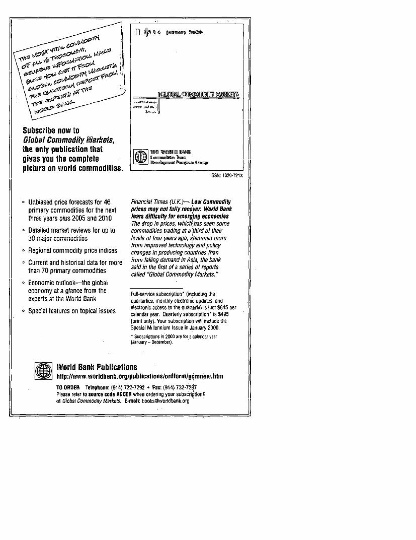
Subscribe now to
l p r - f3n1l l
Globaf l Commodtly i~arketsi,the only publication thatgives tyou- thle'- coml1plete \Upicture on world commodities.
ISSN. 1020-721X
Unbiased price forecasts for 46 Financial Times (U.K.)- Low Commodityprimary commodities for the next prices may not fully recover. World Bankt-hr~eeers pius 2005n and 2010 fears diHIiCultv for emer-ain-g economies
The drop in pres, which, as seen somepDetailed market reviews for up to commodities trading at athird of their
.JU IIIOJUI ~~~~~~~.,UIIIUIUUILIU.~~ISII:102072.
UnA prio, - o- asts for 46ink fniir iagre ann ctomm odf mnry
Regiona commodity price indices from improved technolog W and policythr apr y changes in producing couJntries thanfrom fiimprovemrd itechnologybandkolc
o Current and historical data for more from failiny demand in Asia, the bankthan 70 primary commodities said in the first of a series of reportsthan 70 primary commodities called "Global Commodity Markets."
o Economic outlook-the globaleconomy at a glance from the Full-service subscription' (including the
expei tLs at hle Wor I uDdiIK quarterlies, monthly electronic updates, andelectronic access to the quarterly) is just $645 per
o Special features on topical Issues calendar year. Quarterly subscription* is $495(print only). Your subscription will, include theSpecial Millennium Issue in January 2000.
SubscriDtions in 2000 are for a calendar Year(January - December).
^l World Bank Publicationshtpni/w.w orldbank.orn/lublications/ordform/ cmnew.htm
TO ORDER Telephone: (914) 732-7292 - Fax: (914) 732-7297Please refer to source code AGCER when ordering your subscriptionI:of Global Commodity Markets. E-mall: [email protected]


I F iComing in the next issue of
ITHE WORLD BANKI FlnNnMVTO FiPX7TJEXAT
Ln- *7iinvi 'Onnn
JV- -y A4VV
Volume 14, Number 1
A symposium on trade and technology, including ...I|| *International Knowledge Flows and Economic Performance:An Introductory Survey of the EvidenceGiorgio Barba Navaretti and David TarrI|| *How Trade Patterns and Technology Flows Affect Productivity Growth
Wolfgang KellerAvenues of Technology Transfer: Foreign Investment and ProductivityChange in the Czech RepublicSimeon Djankov and Bernard M. Hoecman
||| *Productivity and Turnover in the Export Market: Micro-level Evidencefrom Taiwan (China) and the Republic of KoreaBee Yan Azv, Sukkyun Chung, and Mark J. Roberts
Vintage Technology and Skill Constraints: Evidence from U.S. ExportsI of New and Used Machinesl JGiorgio barba Navaretti, Iszaro boioaga, and VVenay I akacs
l*Why Agricultural Technology Transfers to Developing CountriesShould Be DeregulatedDavid P. Gisselquist and Jeani-Marie Grether
J A symposium on geographical targeting including.. .th
* Geograph-a 4Tt . P-ve All A
Special IssueDavid Bigman and Hippolyte L. Fofack
* Combining Census and Survey Data to Study Spatial Dimensions ofPoverty: A Case Study of Ecuador
Jesko S. Hentschel, Jean Lanjouzo, Peter F. Lanjouiw, and Javier Poggi| Community Targeting for Poverty Reduction in Burkina Faso
David Bigman, Stefan Dercon, Dominique Guillaume, and Michel Lambotte
| Using Light Monitoring Surveys in Conjunction with Integrated Surveysto Improve Targeting for Poverty Reduction: The Case of Ghana
Hippolyte L. Fofack

L9£t-f IZ8-0 NqSI
Ot9£7 [LZ08L 6 £OS-z ODW
9 H V q )|:\ 1 ]1 ]21) lil X lili S l Ja w w 'H ' S A ae j ea r
_ -- - . .6_ . -. ZOZ_"' . …;.- ' . ' .: -,- r; y R 3 10 Q :l U <
.. ,,. ,. .. i qjr~A~jd1 . :p~p1
*.* )fNVg4rlMOz £Z~Z L3W1 NNVScflOIXK !It'g fl::)Y :xala
-- ZI-LLt (Zoz) :auo d_L
-~ --: ~--- - Y STn 'SEfft2OZ a 'UOl3Uiqsta
- - ; - - -n N '3.aWS H 8 I 8 I
,> j . , . ,: , ; - , , . . .g pp j~ ~ . r


![ACCOUNTABILITY REPORT 2013 › ... › 01 › EDUCO-ACCOUNTABILITY-REPO… · Accountability report 2013 [3]](https://img.pdfslide.us/doc/110x75/5f03b5847e708231d40a62a8/accountability-report-2013-a-a-01-a-educo-accountability-repo-accountability.jpg)