CONF-7905143 Dist. Catg. UC-13, 34b

Workshop on Satellite Power Systems (SPS) Effects on Optical and Radio Astronomy

April 1980

Battelle, Seattle Conference Center Seattle, Washington May 1979

Edited by: P.A. Ekstron and G. M. Stokes Pacific Northwest Laboratory Richland, Washington 99352

Under Contract No. KD-03-82029

Prepared for: U.S. Department of Energy Office of Energy Research Satellite Power System Project Division Washington, D.C. 20545

DOE/NASA

Satellite Power System Concept Development and Evaluation Program

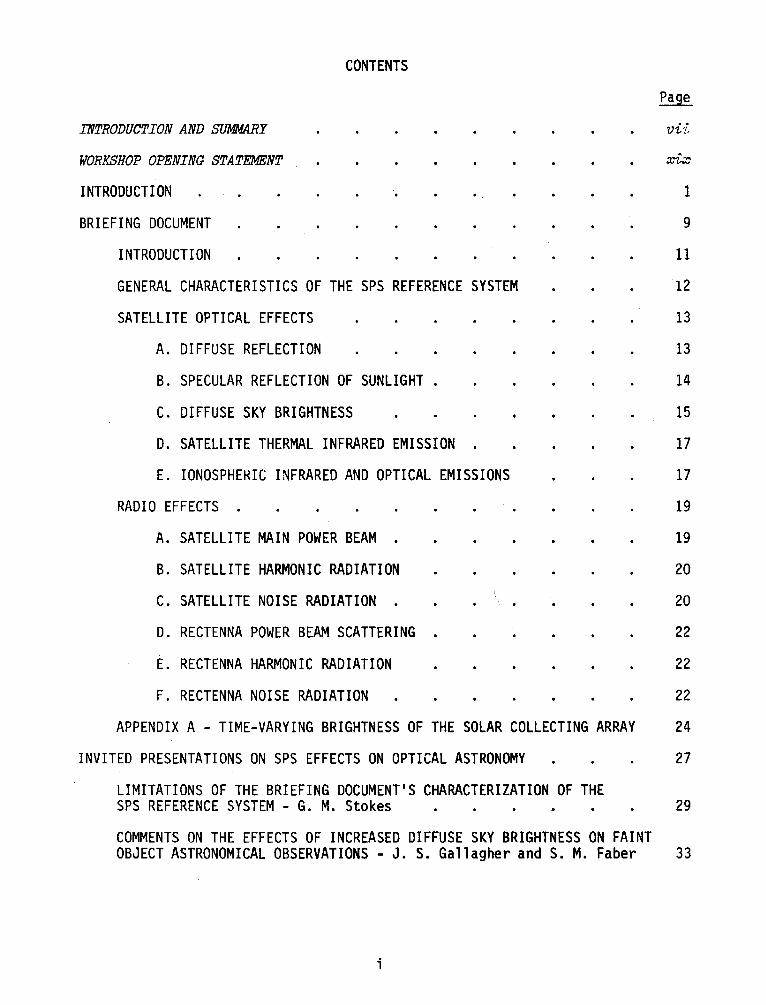
CONTENTS

Page

INTRODUCTION AND SUMMARY vi-t

WORKSHOP OPENING STATEMENT xi:x:

INTRODUCTION 1

BRIEFING DOCUMENT 9

INTRODUCTION 11

GENERAL CHARACTERISTICS OF THE SPS REFERENCE SYSTEM 12

SATELLITE OPTICAL EFFECTS 13

A. DIFFUSE REFLECTION 13

B. SPECULAR REFLECTION OF SUNLIGHT . 14

C. DIFFUSE SKY BRIGHTNESS 15

D. SATELLITE THERMAL INFRARED EMISSION . 17

E. IONOSPHERIC INFRARED AND OPTICAL EMISSIONS 17

RADIO EFFECTS . 19

A. SATELLITE MAIN POWER BEAM . 19

B. SATELLITE HARMONIC RADIATION 20

C. SATELLITE NOISE RADIATION . 20

D. RECTENNA POWER BEAM SCATTERING . 22

E. RECTENNA HARMONIC RADIATION 22

F. RECTENNA NOISE RADIATION 22

APPENDIX A - TIME-VARYING BRIGHTNESS OF THE SOLAR COLLECTING ARRAY 24

INVITED PRESENTATIONS ON SPS EFFECTS ON OPTICAL ASTRONOMY 27

LIMITATIONS OF THE BRIEFING DOCUMENT'S CHARACTERIZATION OF THE SPS REFERENCE SYSTEM - G. M. Stokes 29

COMMENTS ON THE EFFECTS OF INCREASED DIFFUSE SKY BRIGHTNESS ON FAINT OBJECT ASTRONOMICAL OBSERVATIONS - J. S. Gallagher and S. M. Faber 33

;

EFFECTS OF THE SATELLITE POWER SYSTEM ON GROUND-BASED ASTRONOMICAL TELESCOPES - P. B. Boyce . 39

INFRARED ASTRONOMY - D. A. Harper . 45

POSSIBLE IMPACTS OF THE SPS ON THE SPACE TELESCOPE - E. J. Groth 47

REPORT OF THE OPTICAL ASTRONOMY WORKING GROUP 51

THE NATURE OF ASTRONOMICAL OBSERVATIONS . 54

THE ORIGIN OF SPS EFFECTS ON OPTICAL ASTRONOMY 64

IMPACT THRESHOLDS OF THE SPS ON OPTICAL ASTRONOMY 69

EFFECTS ON OPTICAL ASTRONOMY 75

RECOMMENDATIONS AND REMEDIES 77

REPORT ON SPS EFFECTS ON AERONOMY . 81

INTRODUCTION 83

EFFECTS ON AERONOMY OBSERVATIONS - K. Clark 85

INVITED PRESENTATIONS ON SPS EFFECTS ON RADIO ASTRONOMY 95

MICROWAVE POWER TRANSMISSION SYSTEM - G. D. Arndt 97

SPS NOISE AND HARMONICS - R. M. Dickinson 103

SPS-GENERATED FIELD STRENGTHS AT 2.45 GHz TYPICAL EFFECTS -W. Grant . 119

INTERFERENCE EFFECTS ON RADIO ASTRONOMY EQUIPMENT - W. C. Erickson 123

POSSIBLE OVERLOAD AND PHYSICAL DAMAGE OF A RADIO ASTRONOMY RECEIVER CAUSED BY THE SPS - H. Hvatum . 127

POTENTIAL IMPACT OF OUT-OF-BAND RADIATION FROM THE SATELLITE POWER SYSTEM AT ARECIBO OBSERVATORY - M. M. Davis . 131

THE EFFECTS OF THE PROPOSED SATELLITE POWER SYSTEM ON THE VLA -A. R. Thompson . . . ' 135

SATELLITE POWER SYSTEM EFFECTS ON VLBI - B. F. Burke 143

CONSIDERATIONS REGARDING DEEP SPACE COMMUNICATIONS AND THE SPS -N. de Groot 147

ii

REPORT OF THE RADIO ASTROMONY WORKING GROUP 153

SUMMARY STATEMENT 155

ACTUAL PROPERTIES OF THE MICROWAVE POWER TRANSMISSION SYSTEM 158

ASSIGNMENT OF SPS HARMONIC FREQUENCIES . 159

TIME-VARIABILITY OF SPS OFF-AXIS RADIATION AND INTRINSIC MULTIPLE SATELLITE EFFECTS 159

THE "RUSTY BOLT EFFECT" . 160

INTERFERENCE REJECTION PROPERTIES PECULIAR TO SYNTHESIS ARRAYS (AS THE VLA) 161

SITING CONSIDERATIONS 162

ON MOVING RADIO ASTROMONY TO THE LUNAR FAR SIDE 164

APPENDIX A - CCIR REPORTS ON RADIO ASTRONOMY (Reports 223-4 and 224-4) A. l

APPENDIX B - CCIR REPORTS ON DEEP-SPACE RESEARCH (Reports 365-3 and 685) . B. l

APPENDIX C - EFFECT OF SOLAR POWER SATELLITE TRANSMISSIONS ON RADIO ASTRONOMICAL RESEARCH C.l

APPENDIX D - NATIONAL ACADEMY OF SCIENCES REPORT ON SPS EFFECTS . D.l

APPENDIX E - ENVIRONMENTAL CONSIDERATIONS FOR THE MICROWAVE BEAM FROM A SOLAR POWER SATELLITE . E.l

ACKNOWLEDGMENTS 255

iii

WORKSHOP ON SATELLITE POWER SYSTEMS EFFECTS ON OPTICAL AND RADIO ASTRONOMY

Held at BATTELLE SEATTLE CONFERENCE CENTER

May 1979

Edited by GM Stokes

PA Ekstrom

August 1979

Participants

GD Arndt - National Aeronautics and Space Administation B Balick - University of Washington NF Barr - SPS Project Office - DOE P Boyce - American Astronomical Society BF Burke - MIT KC Clark - University of Washington KC Davis - Pacific Northwest Laboratory M Davis - Arecibo Observatory NF de Groot - Jet Propulsion Laboratory RM Dickinson - Jet Propulsion Laboratory PA Ekstrom - Pacific Northwest Laboratory WC Erickson - University of Maryland SM Faber - Lick Observatory, University of California JS Gallagher - University of Illinois W Grant - Institute for Telecommunication Sciences EJ Groth - Princeton University JP Hagen - Pennsylvania State University DA Harper - Yerkes Observatory, University of Chicago WE Howard - National Science Foundation (Division of Astronomical Sciences) AT Moffett - Owens Valley Radio Observatory RO Piland - National Aeronautics and Space Administration GM Stokes - Pacific Northwest Laboratory RA Stokes - Pacific Northwest Laboratory GW Swenson - University of Illinois Observatory AR Thompson - VLA Project - National Radio Astronomy Observatory A Valentino - Argonne National Laboratory

v

INTRODUCTION AND SUMMARY

BACKGROUND

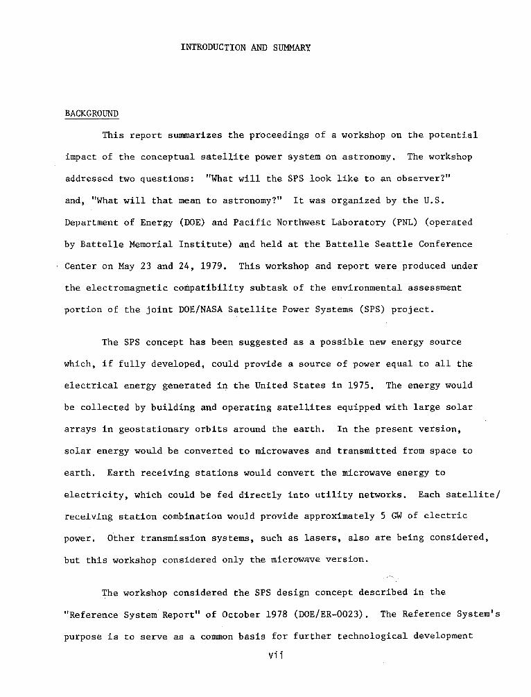
This report sununarizes the proceedings of a workshop on the potential

impact of the conceptual satellite power system on astronomy. The workshop

addressed two questions: "What will the SPS look like to an observer?"

and, "What will that mean to astronomy?" It was organized by the U.S.

Department of Energy (DOE) and Pacific Northwest Laboratory (PNL) (operated

by Battelle Memorial Institute) and held at the Battelle Seattle Conference

Center on May 23 and 24, 1979. This workshop and report were produced under

the electromagnetic compatibility subtask of the environmental assessment

portion of the joint DOE/NASA Satellite Power Systems (SPS) project.

The SPS concept has been suggested as a possible new energy source

which, if fully developed, could provide a source of power equal to all the

electrical energy generated in the United States in 1975. The energy would

be collected by building and operating satellites equipped with large solar

arrays in geostationary orbits around the earth. In the present version,

solar energy would be converted to microwaves and transmitted from space to

earth. Earth receiving stations would convert the microwave energy to

electricity, which could be fed directly into utility networks. Each satellite/

receiving station combination would provide approximately 5 GW of electric

power. Other transmission systems, such as lasers, also are being considered,

but this workshop considered only the microwave version.

The workshop considered the SPS design concept described in the

"Reference System Report" of October 1978 (DOE/ER-0023). The Reference System's

purpose is to serve as a common basis for further technological development

vii

(systems definition and critical supporting investigations), preliminary

environmental and societal assessments, and comparative analyses of the SPS

concept and other national energy ventures. For the most part, the Reference

System is based on fully-matured engineering precepts (methods, materials,

practices, etc.) and realizable projections of future improvements. However,

it is by no means an optimized engineering design, and does not account for

newly emerging technologies which might become standard practices in the

post-2000 era. Continuing systems definition undoubtedly will change many of the

current characteristics of the Reference System. Some of those changes can

already be reasonably perceived, but others most likely will occur that cannot

yet be appreciated. Thus some potential problems associated with the present

Reference System may subsequently become moot, and new one~ will be recognized

as development continues. Despite its current limitations, the Reference

System is an important tool for identifying and evaluating significant

side effects which conceivably could accompany SPS.

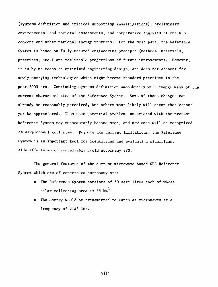
The general features of the current microwave-based SPS Reference

System which are of concern to astronomy are:

• The Reference System consists of 60 satellites each of whose

solar collecting area is 55 km2 •

• The energy would be transmitted to earth as microwaves at a

frequency of 2.45 GHz.

viii

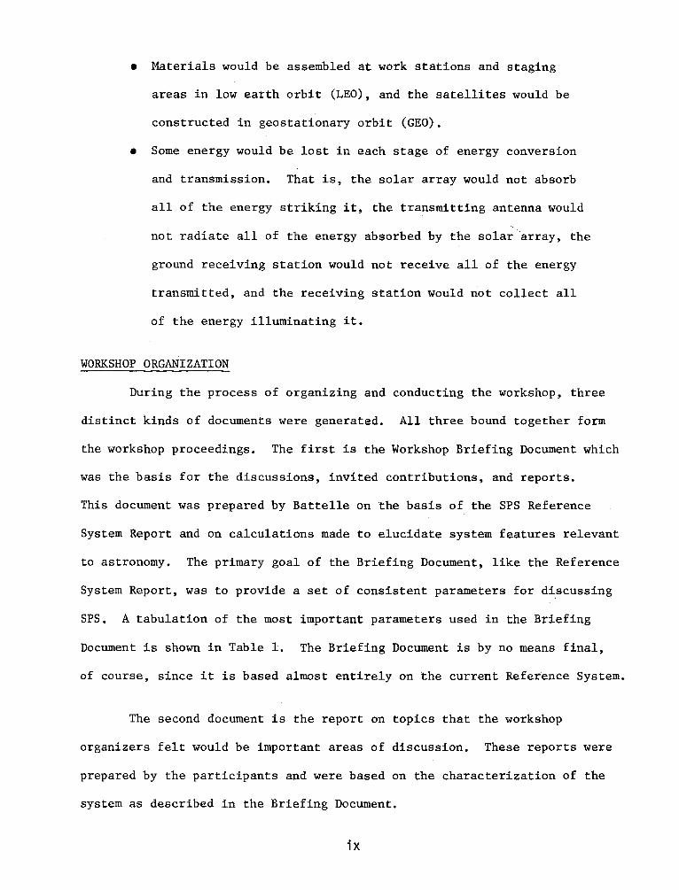
• Materials would be assembled at work stations and staging

areas in low earth orbit (LEO), and the satellites would be

constructed in geostationary orbit (GEO).

• Some energy would be lost in each stage of energy conversion

and transmission. That is, the solar array would not absorb

all of the energy striking it, the transmitting antenna would

not radiate all of the energy absorbed by the solar array, the

ground receiving station would not receive all of the energy

transmitted, and the receiving station would not collect all

of the energy illuminating it.

WORKSHOP ORGANIZATION

During the process of organizing and conducting the workshop, three

distinct kinds of documents were generated. All three bound together form

the workshop proceedings. The first is the Workshop Briefing Document which

was the basis for the discussions, invited contributions, and reports.

This document was prepared by Battelle on the basis of the SPS Reference

System Report and on calculations made to elucidate system features relevant

to astronomy. The primary goal of the Briefing Document, like the Reference

System Report, was to provide a set of consistent parameters for discussing

SPS. A tabulation of the most important parameters used in the Briefing

Document is shown in Table 1. The Briefing Document is by no means final,

of course, since it is based almost entirely on the current Reference System.

The second document is the report on topics that the workshop

organizers felt would be important areas of discussion. These reports were

prepared by the participants and were based on the characterization of the

system as described in the Briefing Document.

ix

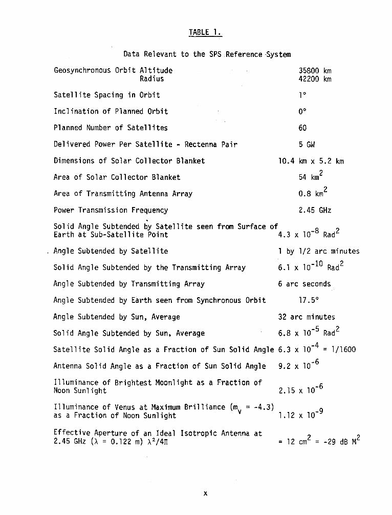
TABLE 1.

Data Relevant to the SPS .Reference -System

Geosynchronous Orbit Altitude Radius

Satellite Spacing in Orbit

Inclination of Planned Orbit

Planned Number of Satellites

Delivered Power Per Satellite - Rectenna Pair

Dimensions of Solar Collector Blanket

Area of Solar Collector Blanket

Area of Transmitting Antenna Array

Power Transmission Frequency .

10.4

35800 km 42200 km

lo

oo

60

5 GW

km x 5.2

54 km2

0.8 km 2

2.45 GHz

km

Solid Angle Subtended by Satellite seen from Surface of 8 2 Earth at Sub-Satellite Point 4.3 x 10- Rad

Angle Subtended by Satellite 1 by 1/2 arc minutes

Solid Angle Subtended by the Transmitting Array 6.1 x lo-10 Rad 2

Angle Subtended by Transmitting Array 6 arc seconds

Angle Subtended by Earth seen from Synchronous Orbit 17.5°

Angle Subtended by Sun, Average 32 arc minutes

Solid Angle Subtended by Sun, Average 6.8 x 10-5 Rad 2

Satellite Solid Angle as a Fraction of Sun Solid Angle 6.3 x lo-4 = 1/1600

Antenna Solid Angle as a Fraction of Sun Solid Angle 9.2 x lo-6

Illuminance of Brightest Moonlight as a Fraction of Noon Sunlight 2.15xl0-6

Illuminance of Venus at Maximum Brilliance (m = -4.3) as a Fraction of Noon Sunlight v 1.12 x lo-9

Effective Aperture of an Ideal Isotropic Antenna at 2.45 GHz (X = 0.122 m) X2/4IT

x

2 2 = 12 cm = -29 dB M

Following an introductory statement, the invited contributions were

presented and discussed. The group was then divided into radio and optical

working groups for more detailed consideration of SPS effects on astronomy.

The form and content of the working group meetings were largely left to the

members of each group with one exception. Both groups were specifically

asked to comment on the possibility of moving the affected portions of

astronomical observations to facilities located in space or on the far side

of the moon. The reports of the working groups make up the final document

in the workshop proceedings.

The objective of the meeting was to identify the potential impacts of

the SPS on astronomy and to do so in a .fashion that would allow system

designers to recognize and modify those aspects of the system that create

potential problems to the extent it may be possible to do so.

The actual content of these various documents fell into two natural

divisions: optical and radio effects. From one viewpoint, this division is

in keeping with an astronomical tradition of dividing the profession according

to the portion of the electromagnetic spectrum that is observed. From another

viewpoint, the division expresses the separate effects of the passive and

active properties of the satellite system. In particular, the major optical

effects caused by SPS would be functions of the system's structures in orbit

and would continue even if the system were turned off. Radio astronomy,

however, would be particularly affected by the active portion of the system

the intended microwave transmission of energy from space to earth. In terms

of design, both optical and radio astronomy impacts are primarily a result

of unintentional side effects. The optical effects would occur because the

SPS solar blankets would reflect some of the light that strikes them. The

radio effects would occur because a small portion of the transmitted energy

xi

would not be confined to the narrow beam from the orbiting antenna to the

earth rectenna, or to the assigned portion of the radio spectrum.

BASIC CONCLUSIONS OF THE WORKSHOP

The effects on astronomy discussed below must be understood in the

general context of how astronomical research is conducted. Participants at

the workshop continually emphasized that virtually all of our knowledge

about the Universe outside of the Solar System has been obtained by studying

the electromagnetic emissions of celestial objects. Because the most distant

objects are also the faintest, all branches of astronomy have attempted to

develop the most sensitive detectors possible. Because these detectors are

so sensitive, they are limited by interference due to other sources of

radiation. The effect of the SPS would be to substantially increase the amount

of man-made interfering radiation. This would further limit the astronomer's

ability to observe faintobjects and thus the size of the measurable Universe.

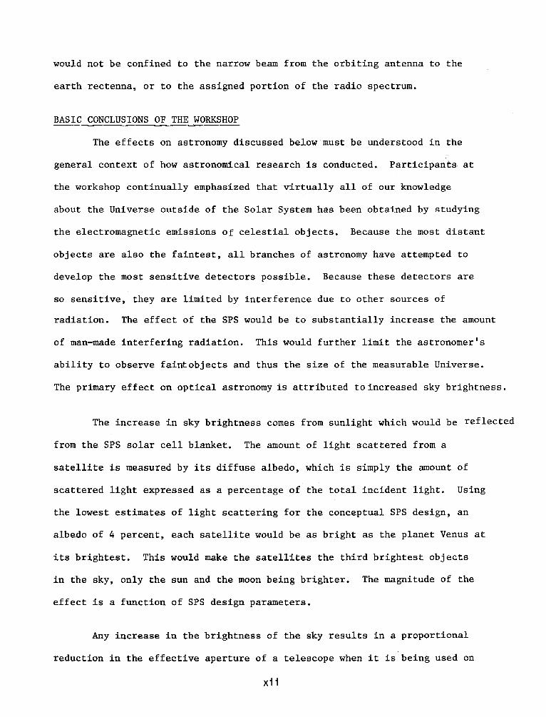
The primary effect on optical astronomy is attributed to increased sky brightness.

The increase in sky brightness comes from sunlight which would be reflected

from the SPS solar cell blanket. The amount of light scattered from a

satellite is measured by its diffuse albedo, which is simply the amount of

scattered light expressed as a percentage of the total incident light. Using

the lowest estimates of light scattering for the conceptual SPS design, an

albedo of 4 percent, each satellite would be as bright as the planet Venus at

its brightest. This would make the satellites the third brightest objects

in the sky, only the sun and the moon being brighter. The magnitude of the

effect is a function of SPS design parameters.

Any increase in the brightness of the sky results in a proportional

reduction in the effective aperture of a telescope when it is being used on

xii

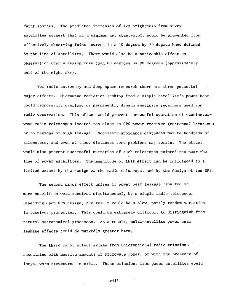
faint sources. The predicted increases of sky brightness from sixty

satellites suggest that at a minimum any observatory would be prevented from

effectively observing faint sources in a 10 degree by 70 degree band defined

by the line of satellites. There would also be a noticeable effect on

observation over a region more than 60 degrees by 90 degrees (approximately

half of the night sky).

For radio astronomy and deep space research there are three potential

major effects. Microwave radiation leaking from a single satellite's power beam

could temporarily overload or permanently damage sensitive receivers used for

radio observation. This effect would prevent successful operation of centimeter­

wave radio telescopes located too close to SPS power receiver (rectenna) locations

or to regions of high leakage. Necessary avoidance distances may be hundreds of

kilometers, and even at those distances some problems may remain. The effect

would also prevent Successful operation of such telescopes pointed too near the

line of power satellites. The magnitude of this effect can be influenced to a

limited extent by the design of the radio telescope, and by the design of the SPS.

The second major effect arises if power beam leakage from two or

more satellites were received simultaneously by a single radio telescope.

Depending upon SPS design, the result could be a slow, partly random variation

in receiver properties. This could be extremely difficult to distinguish from

natural astronomical processes. As a result, multi-satellite power beam

leakage effects-could do markedly greater harm.

The third major effect arises from unintentional radio emissions

associated with massive amounts of microwave power, or with the presence of

large, warm structures in orbit. These emissions from power satellites would

xiii

make the satellites appear as individual stationary radio sources, unlike

natural radio sources. Emissions originating at the power receiving (rectenna)

arrays could be much like other terrestrial sources of interference. Emissions

in the allocated radio astronomy bands are subject to constraints under inter-

national treaty. Emissions at other frequencies can also harm a substantial

number of important radio astronomy observations that occur at spectral lines

and frequencies of opportunity outside the protected radio astronomy bands.

While the potential effects of SPS on astronomical research are quite

diverse, particularly as they apply to the radio and optical regimes of the

electromagnetic spectrum, there are two important effects of common origin

that would affect both areas of research. The satellites would be in geo­

stationary orbits and occupy the same portion of the sky at all times.

Therefore, a fixed region of the sky would not be usable for astronomical

research. The size of the region depends on the design of the satellites,

the particular observation being made, and the kind of instrumentation being

used. The second effect is that the source of electromagnetic interference

and light pollution would be high in the sky. As a result, the general

strategy of placing observatories in remote locations to avoid local interfer­

ence and light pollution effects would be very little help in mitigating SPS

effects on astronomical observations.

Finally, optical effects resulting in increased sky brightness would

affect not only optical astronomy, but aeronomy as well. Aeronomers study

the physics and chemistry of the upper atmosphere by observing naturally

occurring optical emissions such as airglow. This is difficult to distinguish

from other increases in night sky brightness. It was concluded that a

substantial fraction of faint airglow studies are incompatible with the current

SPS Reference System. xiv

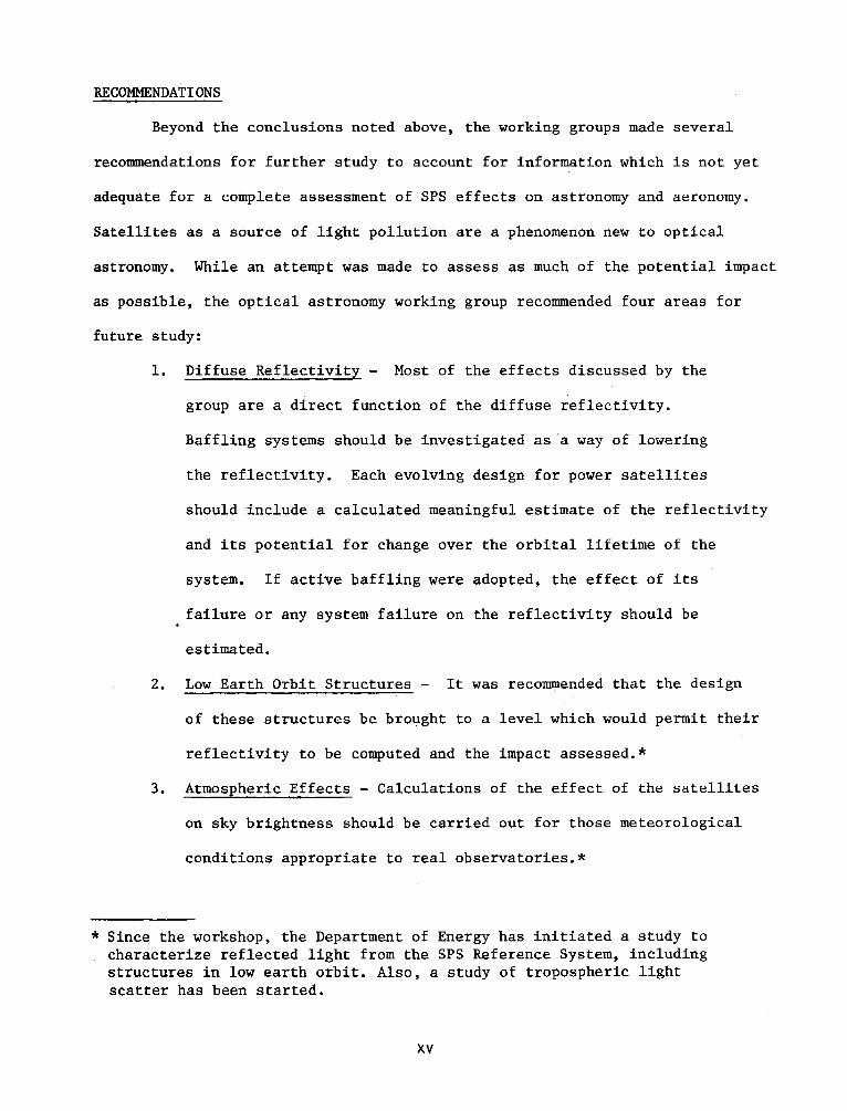
RECOMMENDATIONS

Beyond the conclusions noted above, the working groups made several

recommendations for further study to account for information which is not yet

adequate for a complete assessment of SPS effects on astronomy and aeronomy.

Satellites as a source of light pollution are a phenomenon new to optical

astronomy. While an attempt was made to assess as much of the potential impact

as possible, the optical astronomy working group recommended four areas for

future study:

1. Diffuse Reflectivity - Most of the effects discussed by the

group are a direct function of the diffuse reflectivity.

Baffling systems should be investigated as a way of lowering

the reflectivity. Each evolving design for power satellites

should include a calculated meaningful estimate of the reflectivity

and its potential for change over the orbital lifetime of the

system. If active baffling were adopted, the effect of its

failure or any system failure on the reflectivity should be

estimated.

2. Low Earth Orbit Structures - It was recommended that the design

of these structures be brought to a level which would permit their

reflectivity to be computed and the impact assessed.*

3. Atmospheric Effects - Calculations of the effect of the satellites

on sky brightness should be carried out for those meteorological

conditions appropriate to real observatories.*

* Since the workshop, the Department of Energy has initiated a study to characterize reflected light from the SPS Reference System, including structures in low earth orbit. Also, a study of tropospheric light scatter has been started.

xv

4. Ionospheric Heating - Ionospheric and atmospheric heating

calculations should be used to estimate the effects of

emitted optical and IR radiation on astronomy.

Although a substantial basis already exists for quantitative evaluation

of SPS radio interference, uncertainties concerning properties of SPS and radio

astronomy equipment still remain and in several cases preclude quantitative

estimates of effects. Among the areas the radio group recommended for further

* study were:

1. Noise Radiation - Uncertainties in the noise levels in the protected

bands make it clear that noise measurements for any planned system

should be made at an early stage.

2. Effect on the Very Large Array and Arecibo Facilities - Current

engineering data are not adequate to determine the level of 4.9 GHz

second harmonic interference to these two unique facilities. This

potential problem should be given careful study.

3. Rectenna Siting - Rectenna sites have associated leakage. Its

effect on existing facilities should be investigated.

4. Reradiated Energy - Rectenna arrays would reradiate energy at

various frequencies in the radio spectrum. Their properties are

not yet sufficiently defined to allow a meaningful assessment of the

consequences of this radiation.

Both the optical and radio working groups further recommended an ongoing

panel to continually evaluate the impact of SPS as system designs evolve.

* All these areas are being considered in the current electro-magnetic compatibility task of the SPS Environmental Assessment Program.

xvi

MITIGATION

Due both to the lack of specific SPS data relative to interference

with astronomy and the limited time available for the workshop, mitigation

possibilities were not considered in detail. A specific request was made,

however, to consider the use of space-based facilities to compensate for

interference with earth-based ones.

The discussion of space astronomy as a mitigation strategy was quite

different for each of the two working groups. The optical group noted that

the development of the technology required for the SPS should make it both

easier and cheaper to construct and maintain space telescopes. It is also

recognized that a great deal of the future of astronomy will depend on devel­

oping space astronomy beyond current and planned levels and that some kinds

of astronomy can only be done from space.

Two problems were noted in association with any proposal that space

astronomy might serve as a substitute for lost capability of ground-based

telescopes. First, ground-based facilities have historically been used to

complement those studies made from space, and SPS could affect that interaction

by decreasing the effectiveness of ground-based facilities. Second, it is

important to recognize that astronomy is an observational rather than an

experimental science. It has not always been obvious what the critical

observations are or what the best instruments to pursue them will be. As a

result, the diversity of astronomy has been an important source of vitality in

research. The working group felt that while astronomy) from space is important

and desirable, creating a single space facility to replace ground-based

facilities would not preserve this vitality.

xvii

The radio working group, however, concluded that the reconstruction

and operation of several hundred million dollars' worth of existing ground­

based radio facilities on the lunar farside would be so expensive that it is

not realistic.

The following points were noted with regard to mitigating possible SPS

effects on earth-based observations:

1. Because of SPS's orbital location, distance and terrain cannot

be used to isolate observatories from the source of interference

as has historically been done for earth based interferers. However,

effects on radio observatories could be minimized by providing

maximum separation between them and SPS rectenna sites (expected

to be local interference sources) and locations of strong SPS

microwave leakage.

2. Modification of existing radio astronomy receiving systems to

reduce SPS interference, e.g., by addition of filters, is possible

but would result in some degradation of receiver performance.

As mentioned earlier, SPS is not yet fully developed. Mitigating

strategies appropriate to reducing potential impacts on astronomy should be

accounted for principally by satellite and rectenna designs and engineering

practices, including compliance with regulations governing the shared use of

the electromagnetic spectrum. The early recognition of potential problems,

such as is possible through workshops like the one reported here, is especially

important in providing guiqan~e for future SPS development and electromagnetic

compatibility.

xviii

WORKSHOP OPENING STATEMENT

Ladies and Gentlemen, welcome. In the interest of precision, let me read a short opening statement. It is the last time I plan to read to you.

Our job at this workshop is to elucidate the probable effects of the proposed Satellite Power System on observational astronomy. Each of you invited participants is here for at least two reasons, one technical and one political. Each of you has some technical information or special expertise to contribute to our efforts. Each of you also has experience as a working scientist in one of the areas of observational astronomy which may be affected. You are here not only to contribute information and skill, but also to represent the concerns of your colleagues, to make their voices heard in the complex process of deciding what, how, and whether a Satellite Power System should be.

The output of this workshop will be a report entitled Satellite Power System Effects on Optical and Radio Astronomy. This opening statement will be its preface. About a month ago each of you received a briefing document that outlined our best information on the nature and emissions of the SPS satellites and ground-based components. That document, including any corrections sug­gested here, will form the first major section of the report. A number of you have been asked to prepare presentations on various SPS effects and to bring with you written versions of those presentations. These will form the second major section. The remainder of the re.port will consist of those additional items that you contribute or develop here during the workshop. We have pro­vided the first section and organized the second. The third is yours to write.

As I have said, each of you has an axe to grind. You were chosen because you know and care about some area of observational astronomy. When we called around, asking your colleagues who should represent this or that aspect of the SPS-effects problem, yours were the names which kept cropping up. Presumably you consented to come and work here because you hope to help preserve the environment in which you do your research. To accomplish that goal, we need to answer two questions: "What will the SPS look like to an observer?" and, "What will that mean to astronomy?"

xix

In answering the latter question, bear in mind that this report will be read by many people who do not much care about astronomy, and do not neces­sarily understand the significance and value of data on an object such as a galaxy. It will also be read by persons who care so much about astronomy that no other consideration--such as a society's need for energy--weighs very heavily. If our report is to be influential, both groups must be able to agree that the

issues have been addressed fairly. As you bear in mind this diverse audience, remember as well that any eventual SPS built 20 years from now will likely differ from the Reference System in many ways we cannot now anticipate. The most useful kinds of statements will be those which are not only obviously fair and penetrating, but also easily applied to all future system variants that may be proposed.

We have our work cut out for us.

Thank you.

(These remarks delivered by R. A. Stokes.)

INTRODUCTION

BACKGROUND

This document reports the proceedings of a workshop on the potential impact of the proposed Satellite Power System (SPS) on astronomy. The work­shop was organized by the U.S. Department of Energy (DOE) and Pacific North­

west Laboratory (PNL) (operated by Battelle Memorial Institute) and held at the Battelle Seattle Conference Center on May 23 and 24, 1979. The workshop was conducted and the report prepared under the electromagnetic compatibility subtask of the environmental assessment portion of the joint NASA/DOE Satel-1 ite Power System project.

While the possible effects of the SPS on radio astronomy had been discussed in an initial assessment of the electromagnetic compatibility of the SPS (PNL-2482), it was decided that it would be useful to convene a workshop to more broadly assess the effects on astronomy in general. It was felt that

such a workshop would be the most effective way to involve the astronomical community as a whole in the assessment of SPS. The goal was to keep the investigation of the SPS as open a process as possible. Second, it had become apparent at both DOE and PNL that there were potential adverse effects of the SPS on optical astronomy that did not fall under the clear responsibility of any of the subtasks in the environmental assessment. Responsibility for optical effects was subsequently added to PNL's subtask.

ORGANIZATION OF THE WORKSHOP

The Workshop Briefing Document (see p. 9)provides the basis for the

discussions, invited contributions, and reports that appear in this proceed­ings. This document was prepared by P. A. Ekstrom and G. M. Stokes on the basis of the October 1978 SPS Reference System Report (DOE/ER-0023) and on calculations they made to elucidate system features not well covered in the report. The primary objective of both the Briefing Document and the Reference System Report is to provide a set of numbers that could serve as a point of reference for discussion of SPS. It is essential to understand that the

1

Briefing Document is by no means final. While a conscientious attempt was made to identity and quantify those system parameters that are important to astronomy, the document is based on the reference system. As mentioned in the Briefing Document, major design changes are likely--perhaps as a result of this assess­ment effort--and these changes may affect assumed system properties in a major way. For example, G. D. Arndt's invited presentation includes design changes that reduce grating side lobe intensities by a factor of 10 from those given in the Reference System report.

Many of the workshop participants were asked to prepare reports on specific topics that we felt would be important areas of discussion. These reports were to be based on the characterization of the system as described in the Briefing Document. Each participant was provided with a copy of both the Briefing Document and the Reference System Report about three weeks prior to the work­shop.

The workshop itself was convened with a statement read by R. A. Stokes of PNL which serves as the preface to this report. Following this introductory statement, the invited contributions were presented and discussed. This pro­cess took most of the first day, after which the participants were divided into optical and radio working groups for more detailed consideration of SPS effects on astronomy. The form and content of the working group meetings were largely left to the members of each group with one exception: Both groups were specifically asked to discuss and comment on the possibility of moving the affected portions of astronomical observations to facilities located in space or on the far side of the moon.

ORGANIZATION OF THE REPORT

The entire process of convening, conducting and summarizing this work­shop fell into two natural divisions from the outset. We have, with reason­able accuracy, described these two sections as optical and radio effects, respectively. From one viewpoint, this division is in keeping with an astro­nomical tradition of dividing the profession according to the portion of the electromagnetic spectrum that is observed. From another viewpoint, the division expresses the separate effects of the passive and active properties

2

of the satellite system. In particular, the major optical effects caused by the system are a function of the very existence of the system's structures in orbit and would continue even if the system were turned off. Radio astronomy, however, bears the brunt of the active portion of the system--the intentional transmission of energy to the ground in the form of microwave radiation. In terms of system design, the impacts on both optical and radio astronomy are a result of the fact that SPS is not "perfect". The_ optical effects arise

because the SPS solar blankets will not absorb 100% of the light that strikes them; the radio effects come from the inability to confine all of the trans­mitted energy either to the narrow cone that connects the orbiting antenna to the rectenna on the ground, or to the assigned portion of the radio spectrum.

Another difference between radio and optical astronomy is manifest in their history of dealing with problems such as those presented by the SPS. Radio astronomy is a member of a very large, international community that uses the radio frequency portion of the electromagnetic spectrum. Because these users include both emitters and receivers of radiation that could potentially inter­fere with each other, the spectrum is managed by the International Telecom­munications Union (ITU) which exists by virtue of international treaty. The management process consists of assigning portions of the spectrum to specific classes of users and setting strict standards on the extent to which other users may interfere with certain portions of the spectrum. Radio astronomy has several such bands assigned to it that must be viewed as regions pro-tected by international law. Radio astronomy also has a tradition of vigorous action against those who infringe on these bands. This history of spectrum management has created within radio astronomy a collection of individuals who

are specialists in this area. Many of the workshop participants are such specialists and as a result many of the individuals in the radio astronomy working group had served together on similar committees, discussed the effects of satellites on radio astronomy in other contexts, and discussed SPS pre­viously, with some involved in the writing of the NAS/CORF report.

The legal basis for protection of radio astronomy and the experience of the radio workshop participants had several effects. The standards on interference in the protected bands that the SPS must meet already exist.

3

The group felt that the SPS would have an extremely difficult task meeting these standards. Partly as a result of focusing on the protected bands, the effects on radio observations outside the protected bands may not have been treated in as much detail as might be eventually required. This viewpoint was. in fact, probably the most appropriate one for a workshop of this duration. The section in the radio working group report on the "Rusty Bolt Effect" illus­trates the fact that all of the ways in which the system could create radio frequency interference in protected bands will not be known until the SPS is actually turned on.

Optical astronomy has no such history of enforced protection of observa­tions from interference. Optical astronomers who are interested in faint sources have simply tried to avoid strong sources of light in the planning of their observations and the construction of observatories. They observe at places that are as far removed from large cities as was practical at the time of the construction of the observatory. As with out-of-band radio astronomy, terrain shielding is the method by which optical astronomers attempt to pro­tect their observations from interference. Because of this difference in the

history of optical and radio astronomy, existing light pollution standards for optical astronomy are few and have sanction under municipal law only in iso­lated instances. There are very few light pollution specialists in optical astronomy. As a result, much of the discussion of the optical group centered on setting reasonable standards for light pollution that could be used in this assessment of SPS effects. The concept of ''impact thresholds'' was developed in this context, and whereas it does not have the quantitative basis that the radio regulations do, the concept should be useful in assessing satellite designs.

A final major difference between the optical and radio working group reports can be found in the extensive discussion of the conduct of optical astronomical observations. The optical working group felt that it was nec­essary to provide sufficient background to allow someone unfamiliar with astronomy to understand the working group report. On the other hand, since the radio working group felt that the discussion of astronomy in the CCIR 224-4 report served the same function for its report, the CCIR report is included here as an appendix to the radio astronomy section.

4

Once the optical astronomy working group convened, it became increasingly clear that optical aeronomy, represented by K. Clark of the University of Washington, deserved attention beyond that which could be provided in the optical astronomy report. As such, aeronomy has been separated out as a third topic of the workshop. This separation is quite appropriate because a large

fraction of the natural background sky brightness comes from aurorae and air­glow phenomena studied by aeronomers. Since the effects studied produce relatively diffuse light emission which is especially difficult to distinguish from other increases in sky brightness, the thresholds for impacts on aeronomy are lower than they would be for optical astronomy.

BASIC CONCLUSIONS OF THE WORKSHOP

While the effects of the SPS on astronomical research are quite diverse, particularly as they apply to the radio and optical regimes of the electro­

magnetic spectrum, there are two important effects that have a common origin that will affect both areas of research. The geostationary character of the satellite orbits means that the satellites will occupy the same portion of the sky at all times. Therefore, a fixed region of the sky will be unusable for astronomical research. How large this region is depends on the design of the satellites, the particular observation being made, and the kind of instrumen­tation being used. A further effect is that placing the source of electro­magnetic interference and light pollution relatively high in the sky will essentially eliminate terrain shielding as a strategy to combat pollution and

interference effects.

The primary effect on optical astronomy was attributed to increased sky brightness. Any increase in the brightness of the sky results in a propor­tional reduction in the effective aperture of a telescope when it is being used on faint sources. The predicted increases of sky brightness suggest that at a minimum any western hemisphere observatory will be prevented from effec­tively observing faint sources in a region that covers 10° in declination and 70° in hour angle surrounding the line of satellites. There will also be, again as a minimum, a noticeable effect on observation over a region that covers more than 60° in declination and 90° in hour angle, approximately half

5

of the night sky. The magnitude of this effect is a strong function of SPS design parameters, and it appears that for more likely design parameters, in particular for a likely increase in the diffuse albedo of the satellites, the effect will be much greater.

For radio astronomy and deep space research there are three major effects. Microwave radiation leaking from a single satellite's intentionally generated power beam can temporarily overload or permanently damage the sensitive receivers used for radio observation. This effect will prevent successful operation of centimeter-wave radio telescopes located too close to power receiver (rectenna) locations or to regions of high leakage (grating side lobes). Necessary avoidance distances may exceed hundreds of kilometers. The effect will also prevent successful operation of such telescopes pointed too near the line of power satellites. The magnitude of this effect can be influenced to some extent by the design of the radio telescope, and to a smaller extent by the design of the SPS.

The second major effect arises when power beam leakage from two or more satellites is received simultaneously by a single radio telescope. The result will be a slow, partly random variation in receiver properties that can be extremely difficult to distinguish from the astronomical process being observed. As a result, power beam leakage effects will do markedly greater harm when more than one satellite is operating simultaneously.

The third major effect arises from unintentional radio emissions unavoid­ably associated either with the generation and handling of massive amounts of microwave power, or with the presence of large, warm structures in orbit. When these emissions originate in the power satellites, they make the satel­lites appear as individual radio sources that do not move as do natural radio sources. When the emissions originate in the power receiving (rectenna) arrays, they can be much like other terrestrial sources of interference. When these emissions lie in the allocated radio astronomy bands, they are subject to the most stringent regulations under international treaty. These regulations may prove extremely difficult for the system to meet. When the emissions occur at other frequencies, they are subject to less stringent

6

standards but can still do comparable harm to the substantial amount of impor­tant radio astronomy observation that occurs at spectral lines and frequencies of opportunity outside the protected radio astronomy bands.

Although a substantial basis already exists for quantitative evaluation of the SPS radio interference, specific uncertainties concerning properties of the SPS and of radio astronomy equipment still remain and in several cases preclude quantitative estimates of effects. The report of the radio working group offers those quantitative estimates that can be made now, makes a number

of recommendations for further investigation, and urges that an ongoing panel be constituted to evaluate the impact of SPS as the design of the system evolves.

SPACE POWER SATELLITE BRIEFING DOCUMENT-­RADIO AND OPTICAL ASTRONOMY EFFECTS

INTRODUCTION

SPACE POWER SATELLITE BRIEFING DOCUMENT-­RADIO AND OPTICAL ASTRONOMY EFFECTS

This briefing document was prepared for participants in a workshop on Satellite Power System (SPS) effects on optical and radio astronomy held May 1979 in Seattle, Washington. The document draws much of its information from, and is meant to be used in conjunction with, the SPS Reference System Report, DOE/ER-0023, dated October 1978. The aim of this Briefing Document is to collect information relevant to SPS effects on optical and radio astronomy, to present the information in a manner that is both useful to the astronomical observing communities, and is as independent as possible of future changes in the SPS design.

In most cases, the numerical quantities of greatest interest are not given in the Reference System Report and had to be calculated or estimated based on information that was available. In such cases, the numbers were calculated in the simplest manner consistent with a useful result. Results of more than one significant figure are seldom offered for a quantity. Greater emphasis has been given to the identification of qualitative effects, and some effects are mentioned for which no magnitude estimate is currently available.

In view of probable SPS design changes and uncertainties in the pro­perties of some system components, it is important to regard the information presented here as reference numbers used to focus discussion, and not as definitive results. These same uncertainties mean that the most useful and influential statements on SPS effects will be those phrased in one of two ways: they either should be parametric in the level of SPS emission or should offer design criteria to be observed if corresponding effects are to be avoided. Persons evaluating SPS effects are encouraged to report their conclusions in one of these two forms whenever possible.

11

GENERAL CHARACTERISTICS OF THE SPS REFERENCE SYSTEM

The Reference System consists of 60- sate 11 ites in synchronous orbit, each consisting of a large (54-km2), solar photovoltaic cell array and a microwave beam generator used to transmit power to an antenna-rectifier ( 11 rectenna 11

)

array on the earth's surface. Each satellite transmits 6.7 GW (109 W) at 2.45 GHz, and delivers a nominal 5 GW to the utility power grid. Pages 10-46 of the Reference System Report, DOE/ER-0023, provide a good introduction to the system, and should be read by anyone unfamiliar with the details of the Reference System.

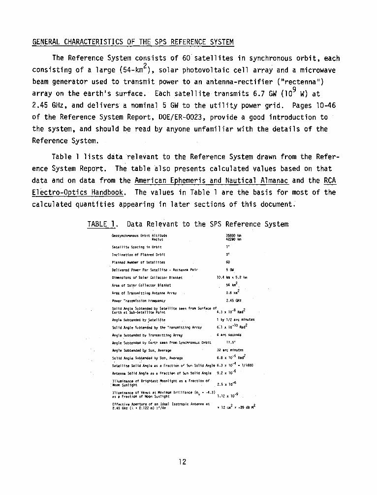
Table 1 lists data relevant to the Reference System drawn from the Refer­ence System Report. The table also presents calculated values based on that data and on data from the American Ephemeris and Nautical Almanac and the RCA Electro-Optics Handbook. The values in Table 1 are the basis for most of the calculated quantities appearing in later sections of this document.

TABLE 1. Data Relevant to the SPS Reference System Geosynchronous Orbit Alt1t1.ule

Rodi us

Sa tell 1te Spacing in Orbit

Inclination of Planned Orbit

Planned Number of Satell 1tes

Delivered Power Per Satellite - Rectenna Pair

Dimensions of Solar Collector Bl•nket

Area of so1.ar Collector 6lanket

Al"ea of Transmitting Antenna Array

Power Transmission Frequency

35800 km 42200 1<11

l"

o•

60

5 GW

10.4 km x 5.2 1<11

54 km2 .

0.8 km2

2 .45 GHZ

~~~~~ :~g~b~~~~=~~~e bi0~~~ell i te seen from Surface of 4_3 x 10_8 Rad2

Angle Subtended by .Satell~te l by l/2 arc 11inutes

Solid Angle Subtended by the Transmitting Array 6. l x 10-lO Rad2

Angle ,,subtended by Transmitting Array 6 •re: seconds

Angle Subtended by E~rth seen from Synchronous Orb1t 17 .S"

Angle SUbtended qy Sun, Average 32 arc minute•

Solid Angle Subtended by Suo, Average 6.8 x 10-S Rad2

Satellite Solid A.ngle as a Fraction of Sun Solid Angle 6.3 x 10·4 = l/1600

Anteooa Solid Angle as a Fraction of Sun Solid Angle 9.2 x 10"6

11 luminance of Brightest Moonlight as a Fraction of Moon Sunlight 2.5 x 10·6

Illuminance of Venus at MaxillW,lm Brilliance (mv • -4.3) _9 as ~ Fraction of Noon Suol ight 1.12 x 10

E:ffective Aperture of an Ideal Isotropic Antenna at • 12

cm2 • _29

dB H2 2.45 GHz (A • 0.122 m) A'/4w

12

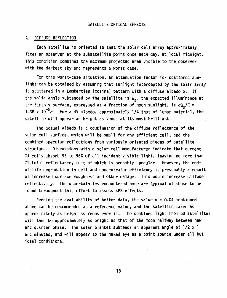
SATELLITE OPTICAL EFFECTS

A. DIFFUSE REFLECTION

Each satellite is oriented so that the solar cell array approximately faces an observer at the subsatellite point once each day, at local midnight. This condition combines the maximum projected area visible to the observer with the darkest sky and represents a worst case.

For this worst-case situation, an attenuation factor for scattered sun-1 ight can be obtained by assuming that sunlight intercepted by the solar array is scattered in a Lambertian (cosine) pattern with a diffuse albedo a. If the solid angle subtended by the satellite is ns' the expected illuminance at the Earth's surface, expressed as a fraction of noon sunlight, is ans/IT = 1.38 x l0-8a. For a 4% albedo, approximately 1/4 that of lunar material, the satellite will appear as bright as Venus at its most brilliant.

The actual albedo is a combination of the diffuse reflectance of the solar cell surface, whicn will be small for any efficient cell, and the combined specular reflections from variously oriented pieces of satellite structure. Discussions with a solar cell manufacturer indicate that current Si cells absorb 93 to 96% of all incident visible light, leaving no more than 7% total reflectance, most of which is probably specular. However, the end­of-1 ife degradation in cell and concentrator efficiency is presumably a result of increased surface roughness and other damage. This would increase diffuse reflectivity. The uncertainties encountered here are typical of those to be found throughout this effort to assess SPS effects.

Pending the availability of better data, the value a = 0.04 mentioned above can be recommended as a reference value, and the satellite taken as approximately as bright as Venus ever is. The combined light from 60 satellites will then be approximately as bright as that of the moon halfway between new and quarter phase. The solar blanket subtends an apparent angle of 1/2 x 1 arc minutes, and will appear to the naked eye as a point source under all but ideal conditions.

13

B. SPECULAR REFLECTION OF SUNLIGHT

Both the solar cell blanket and the transmitting antenna array have large, flat specularly-reflecting surfaces. Although the antenna array is much smaller, 0.8 km2 versus 54 km2, its expected reflectance is much greater, leading to comparable estimated illumination levels at the Earth's surface for reflections from each surface. The antenna's aluminum front surface is expected to have a specular reflectance above 0.9. Of the various possible reflecting interfaces in the solar blanket, the boundary between vacuum and front cover sheet is easily analyzed and can be used to set a lower bound to array reflectance. The silicon cell option employs a borosilicate glass cover sheet with a reflectance of 0.04. The GaAlAs option employs synthetic sapphire with a reflectance of 0.063, but at a concentration ratio of two, so that only half of the blanket area is cover sheet. The effective reflectance for the GaAlAs option is therefore 0.032. We adopt a mean value of 0.036.

The reflected spot of light on the surface of the Earth may be regarded as a pinhole earner~ image of the Sun approximately 330 km in diameter. It will be reduced in brightness from that of noon sunlight by the product of the specular reflectance of the surface and the ratio of solid angle subtended by the satellite to that subtended by the Sun's disk. For the solar blanket, the illumination as a fraction of noon sunlight is 2.3 x 10-5, or approximately ten times that of brightest moonlight. For the antenna array, the fractional illumination is 8 x 10-6, roughly four times that of brightest moonlight.

If the solar blanket were held precisely facing the Sun, then specular reflection from it could fall on the Earth only for the brief period when the satellite was in the Earth's penumbra, and would be visible only at local sunset or sunrise. If the satellite's attitude is controlled only well enough to avoid significant power loss, the reflected spot could fall on a much larger portion of the Earth's night side.

The transmitting antenna is constrained by beam-forming requirements to point with high precision directly toward its rectenna array. The path of the reflected spot across the surface of the Earth is, therefore, completely determined once the longitude of the satellite and location of the rectenna are specified. Livingston (L. E. Livingston, Visibility of Solar Power Satellites from the Earth, Document JSC-14715, L. B. Johnson Space Center,

14

Houston, TX, Feb. 1979) has analyzed the situation and concludes that each antenna's reflected spot will illuminate any given observer on approximately two successive nights in the spring and two in the summer. The period of illumination can be as long as 2 minutes and, as mentioned above, will be significantly brighter than the full moon.

It should be noted that this illumination comes from a much smaller object and corresponds to a much larger surface brightness than that of the moon. The surface brightness is expected to be just the reflectivity of the satellite times the surface brightness of the Sun. High-surface brightnesses are of special concern regarding possible local damage to the photosensitive surface of any imaging optical detector that can resolve or nearly resolve the satellite. As one example, the dark-adapted human eye may be at risk.

C. DIFFUSE SKY BRIGHTNESS

Increases in diffuse s~ brightness are expected from either the diffuse reflection from the solar collector or the specular reflection from the antenna. The effects of these two phenomena are quite different.

The diffuse reflection is a persistent effect. The satellites always occupy the same position in the sky, with their apparent brightness varying with time as described in the appendix. The apparent positions of the indi­vidual satellites, for a 60-satellite system, as seen from Kitt Peak, Cerro Tololo, and Mauna Kea are shown in Figure 1.

The net effect of the diffuse brightness of these satellites can be estimated using ~van King's study of the profile of stellar images (Publi­cations of the Astronomical Society of the Pacific, Volume 83, p. 199, 1971). He found that well away from a star the sky brightness falls off as r2, such that the sky brightness around an object, in magnitudes per square second of arc, is given by

m(sky) = m(obj) + 7.5 + 5 log r

where m(obj) is the apparent visual magnitude of a satellite's solar blanket, and r is the angular separation in arc seconds. The total contribution of the Reference System to diffuse sky brightness is, therefore, simply the super­position of the effects of the 60 satellites.

15

z 0

!;( 0. QO -z -I u ...... 0

~

-100 -

MKO

I I I

600 300 EAST

KPNO

I

oo HOUR ANGLE

CTIO

I I

300

FIGURE 1. Apparent Satellite Positions for 60-Sattellite System as Seen from Three Major Observatories

I

900 WEST

If we assume the maximum brightness of individual satellites is equal to that of Venus, mv = -4.3, then observatories located in longitudes 70° to 130° will experience some deterioration in quality of dark-time observing. The additional sky brightness from SPS for these observatories would exceed the average dark sky brightness, mv - 22/sq. second of arc, for a zone which crosses the meridian and covers more than 70° in hour angle and up to 10° in declination. This zone would have a sharply peaked ridge of emission centered on the apparent position of the array of satellites, such that within a 3° wide band the sky is five times brighter than dark night sky and within ±20 minutes of arc the effect is more than 10 times that of the dark sky.

When the specularly reflected beam from the microwave-transmitting antenna

is illuminating ground features or part of the atmosphere visible from an observatory, multiple scattering (or single scattering when the beam passes overhead) can contribute additional diffuse sky brightness. The magnitude of

this effect has not been calculated, even for the best case of a dust-free

16

cloudless night. The effect will occur whenever the specular beam from any of

the 60 satellites passes sufficiently near an observing site: presumably, once

per night for several minutes for the few days preceding and following the direct illumination of the site by each satellite.

D. SATELLITE THERMAL INFRARED EMISSION

Both the GaAlAs and the Si cel1 solar blankets absorb about 50 GW more power as sunlight than they deliver as electrical output. This excess power

is radiated in the infrared from both sides of the blanket. For an assumed Lambertian pattern,

I = 50 GW/2Il ~ 8 GW/Rad2

power incident per unit area on Earth is

The GaAlAs cells cover about half the area of the array (the rest in concentra­tor) and operate at 125°C, which is associated with a blackbody peak at 6.9 microns. The Si cells operate at 36.5°C for a blackbody peak at 8.8 microns.

The actual spectral distribution of the radiation will depend on the wavelength dependence of solar cell emissivity, as determined by the details

of anti-reflection coatings, etc.

E. IONOSPHERIC INFRARED AND OPTICAL EMISSIONS

Transmission of the microwave beam is expected to raise the electron tem­perature to a peak of at least 950 K throughout the D- and E-region of the ionosphere, causing a significant perturbation in the ambient conditions along the beam. Electron energy loss mechanisms will produce some enhancement of 6300A airglow emissions from 0( 1D) and 4.3-µ and 6.5-µ infrared emissions from

17

co2 and H20, respectively. Diurnal variations are significant, and quantita~ tive estimates of the intensity of these emissions are not readily available at present. If these particular line emissions pose a special problem for obser­vational work, a determination of the maximum permissible enhancement should be made.

18

RADIO EFFECTS

A. SATELLITE MAIN POWER BEAM

The power transmission beam, 6.7 GW at 2.45 GHz, is the satellite's dominant microwave emission. Concern over possible ionospheric heating effects has resulted in a limitation of the microwave power densities within the transmitting beam to a maximum of 23 milliwatts/cm2. At the perimeter of the rectenna array power density will be approximately l milliwatt/cm2. Power density far from the beam center depends critically on details of the transmitting array design, but is nominally 2 microwatts/m2 as far as one Earth radius away from the beam center. In addition, design-dependent isolated subsidiary peaks (grating lobes) of~ l watt/m2 power density will occur at intervals of 440 km along an east-west line through the main beam; this line will be repeated at comparable intervals (stretched at high latitudes by projection effects) north and south. Figures 19 through 22 of the Reference System Document and the accompanying text give further details on expected power densities.

An ideal isotropic antenna (O dB gain) has an effective aperture of 12 cm2 at 2.45 GHz. Such an antenna mounted on an aircraft or satellite passing through the center of the main beam could intercept and deliver to the receiver terminals approximately 1/4 watt of power, which is sufficient to damage many receivers. An isotropic antenna located 1 Earth radius away from a beam center would intercept 2.5 nanowatts per operating satellite. An antenna with 1/2 m2 effective aperture, e.g., a 26-dB radio telescope side lobe, could deliver one rnicrowatt, which is sufficient to overload many parametric amplifiers.

The frequency of the main power beam must be very stable in order to avoid unintentional frequency-scanning of the beam by the transmitting phased array. Amplitude stability is only loosely constrained by system requirement'. and will depend on details of satellite D.C. power switch-gear and on the power control strategy adopted. T~~ Reference System Report gives no values for either stability.

19

The beam center frequency choice of 2.45 GHz is a reasonable one from many viewpoints. Nonetheless, no international frequency assignment has been made, and this choice cannot yet be considered final.

B. SATELLITE HARMONIC RADIATION

Any microwave power generator can be expected to produce some power at frequencies harmonically related to the main frequency generated. For the klystron tubes of the Reference System, the fraction of output power appearing as harmonics is expected to be small, but no values are given. The radiation pattern of the transmitting phased array when driven at harmonic frequencies is very dependent on details of feed design, and again no information is given. Nonetheless, the large powers involved mean that even a fractionally small diversion of power into harmonics could be significant, and persons evaluating potential effects should attempt to determine effect thresholds at the first few integer multiples of 2.45 GHz.

C. SATELLITE NOISE RADIATION

At frequencies far removed from the beam center frequency, the dominant microwave radiation source will be thermal emission from the hot solar cell blanket. A 330-Kelvin blackbody radiator (case of Si cells, microwave emissivity= l) in the Rayleigh-Jeans limit has a surface brightness of 7.3 x lo- 19 W/m2 Hz Rad2 at 2.45 GHz. Since the solar cell blanket subtends 4.32 x 10-8 Rad2, this surface brightness results in a noise power density at the Earth's surface of 3.16 x l0-26 W/m2 Hz, or -255 dB W/m2 Hz. This density should be multiplied by the actual microwave emissivity of the cell blanket, a number less than unity. Unless the emissivity is very small, it will not affect the qualitative conclusions below.

Figure 26 of the Reference System Report shows an actively radiated noise power density equal to -255 dB W/m2 Hz at 70 MHz away from the beam center frequency, rising rapidly as the center frequency is approached. The central plateau region is a factor of 10

6 (60 dB) brighter.

Since the transmitting antenna is a much smaller object than the blanket, this brightness comparison is valid only for an antenna whose main beam is at

20

least as large as the cell blanket. A beam solid angle of 4.3 x 10-8

Rad2 or less implies a directivity greater than 84 dB and, at these frequencies, an effective aperture greater than 3.4 x 105 m2. The Arecibo dish has an aperture only twice this large, and all other single dishes are smaller.

Interferometers which can just resolve the 0.8 km2 transmitting antenna will see it become brighter than the blanket over a band extending approxi­mately 140 MHz on each side of the center frequency. Further increases in resolution will eventually reveal the transmitting array center to be 2.5 times brighter because of illumination taper.

The total integrated noise power implied by the spectrum of Figure 26 is approximately 5 x lo-13 W/m2.

The calculation reported as Figure 26 (G. D. Arndt and L. Leopold, 11 Environmental Considerations for the Microwave Beam from a Solar Power Satellite, 11 13th Intersociety Energy Conversion Engineering Conference, San Diego, CA, August 1978) implies a noise beam width approximately 100 times larger than the power beam width. Frequency scanning effects are neglected, as is any noise contribution to the klystron drive source. To date, no one has constructed a prototype SPS klystron. All noise data are extrapolated from performance of existing tubes both with respect to tube construction and with respect to frequency dependence in the wings of the noise spectrum. It is difficult for us to assess the reliability of these extrapolations.

Although not currently part of the Reference System, both amplitron tubes and solid-state devices are being seriously considered in some quarters as alternatives to klystrons. Of the two, the amplitrons are inherently much noisier devices with much broader emissions, and are most convenient to apply in cascades which are significantly noisier than individual tubes. A variety of solid-state devices is being considered, and the present rapid rate of device development may well make available entirely new devices in the decade or more which will elapse before the transmitter design must be frozen. As a result, the formulation of effects statements suggested in the introduction, either as parametric in system properties or as effect thresholds, is especially important for noise effects.

21

D. RECTENNA POWER BEAM SCATTERING

Although designed to efficiently absorb the incident power beam, the rectenna structure will inevitably reflect and scatter some small percentage of the beam power. The 2.45-GHz power density in its immediate vicinity will, therefore, be somewhat larger and more complicated in structure than is implied by the transmitting antenna 1 s beam pattern. This is not expected to be a large effect, although no magnitude estimates are given.

E. RECTENNA HARMONIC RADIATION

The rectenna can be expected to radiate harmonic energy originating in its rectifying diodes; This is recognized to be a problem both for power conversion efficiency and for EMI effects, and low-pass filters have been incorporated into the more recent rectenna designs. Details of the rectenna are still in flux, but initial measurements on one prototype (Arndt and Leopold, op. cit. p. 21) showed that power re-radiated at the second' har­monic (4.9 GHz) was 25 dB below the incident power. This corresponds to re-radiation of 21 MW from a rectenna illuminated by a 6.7 GW beam. Third and fourth harmonics were found to be 40 dB and >70 dB below incident power, corresponding to re-radiation of 670 KW and less than 670 W, respectively.

Harmonic radiation from individual dipole elements should be partially coherent across the rectenna array, leading to formation of beams. Their detailed structure will depend in turn upon the details of the partial coherence of the incident power beam, and will be time-varying.

Again, the most useful statements to be made concerning harmonic radiation effects are those which are parametric in harmonic signal strength, or are effect thresholds.

F. RECTENNA NOISE RADIATION

The fraction of incident power absorbed by the rectenna dipoles depends on the accuracy of their impedance match with the rectifier diodes, and that in turn depends on the rectenna D.C. bus voltage and diode current. There­fore, any variation in system bus voltage, e.g., as a result of cyclic

22

commutator loading or switchgear operation, and any fluctuation in diode current, e.g., as a result of wideband internal diode noise sources, will

modulate the reflected power and radiate noise sidebands. Although no magnitude estimate is given for this effect, the radiated noise can be expected to most strongly affect those installations within a few rectenna diameters (10 km) of a rectenna.

23

APPENDIX

TIME-VARYING BRIGHTNESS OF THE SOLAR COLLECTING ARRAY

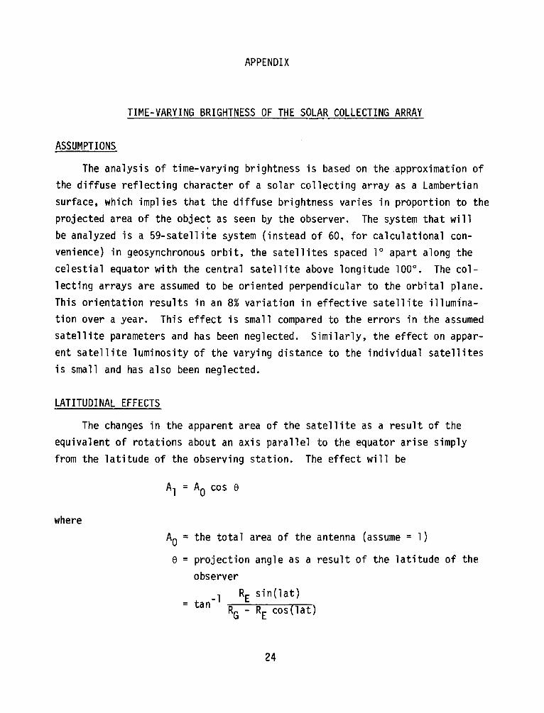
ASSUMPTIONS

The analysis of time-varying brightness is based on the approximation of the diffuse reflecting character of a solar collecting array as a Lambertian surface, which implies that the diffuse brightness varies in proportion to the projected area of the object as seen by the observer. The system that will be analyzed is a 59-satellite system (instead of 60, for calculational con­venience) in geosynchronous orbit, the satellites spaced 1° apart along the celestial equator with the central satellite above longitude 100°. The col­lecting arrays are assumed to be oriented perpendicular to the orbital plane. This orientation results in an 8% variation in effective satellite illumina­tion over a year. This effect is small compared to the errors in the assumed satellite parameters and has been neglected. Similarly, the effect on appar­ent satellite luminosity of the varying distance to the individual satellites is small and has also been neglected.

LATITUDINAL EFFECTS

The changes in the apparent area of the satellite as a result of the equivalent of rotations about an axis parallel to the equator arise simply from the latitude of the observing station. The effect will be

where A0 =the total area of the antenna (assume= l)

e = projection angle as a result of the latitude of the observer

= tan-l RE sin(lat) RG - RE cos(lat)

24

with RE = the radius of the Earth

RG = the radius of the geosynchronous orbit.

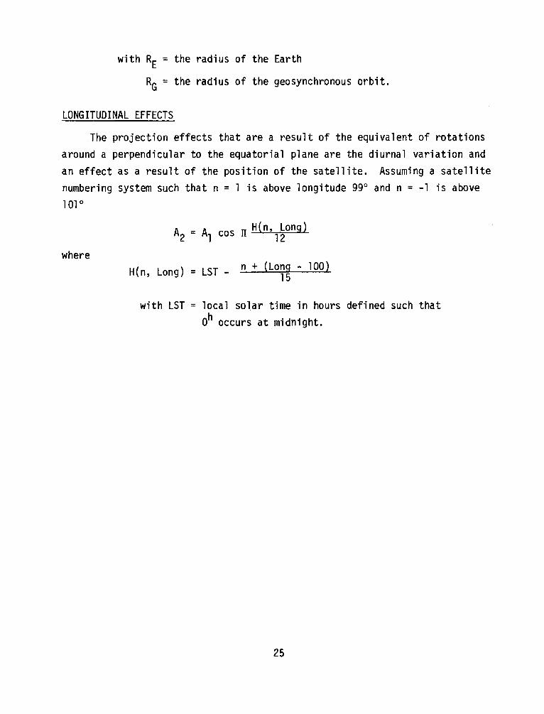
LONGITUDINAL EFFECTS

The projection effects that are a result of the equivalent of rotations around a perpendicular to the equatorial plane are the diurnal variation and an effect as a result of the position of the satellite. Assuming a satellite numbering system such that n = l is above longitude 99° and n = -1 is above l 01°

where H(n, Long) = LST - n + (Lo~g - lOO)

with LST = local solar time in hours defined such that oh occurs at midnight.

25

INVITED PRESENTATIONS ON SPS EFFECTS ON OPTICAL ASTRONOMY

LIMITATIONS OF THE BRIEFING DOCUMENT'S CHARACTERIZATION OF THE SPS REFERENCE SYSTEM

G. M. Stokes

Virtually all of the major effects of the SPS on optical astronomy, infrared astronomy and aeronomy arise from what can be called the passive properties of the SPS. That is to say, the effects are not a result of what the system does, but rather a result of the simple existence of the system. Tbe ~haractert~ation of the Reference System in the Briefing Document repre­sents our best estimate of what a 60-satellite system will look like. In order to assess the effects of the passive properties of the system on astro­nomy and aeronomy, it is important to understand the limitations of the Briefing Document assessments.

The effect of primary interest, i.e., the increase in diffuse sky bright­ness, has origins in both the system design and the propagation of light through the atmosphere. There are at present four areas in which the Briefing Document description may be subject to alteration:

l. The Albedo Estimate - The adopted value of 4% may be wrong by as much as a factor of two. Values in the range 2 to 10% have been quoted and no real estimate exists of the change in albedo as the system is aged through micrometeoritic bombardment.

2. The Satellites Were the Only Structures Considered - One feature of the reference system is a low Earth orbit (LEO) support area. This structure or structures could be very bright, and because of its orbit, it would be a great detriment whenever visible.

3. Glints from the Support Structure - In computing the apparent visual magnitude of the system, a contribution from specular glints from the support structures were not included. Their effect may be

large.

29

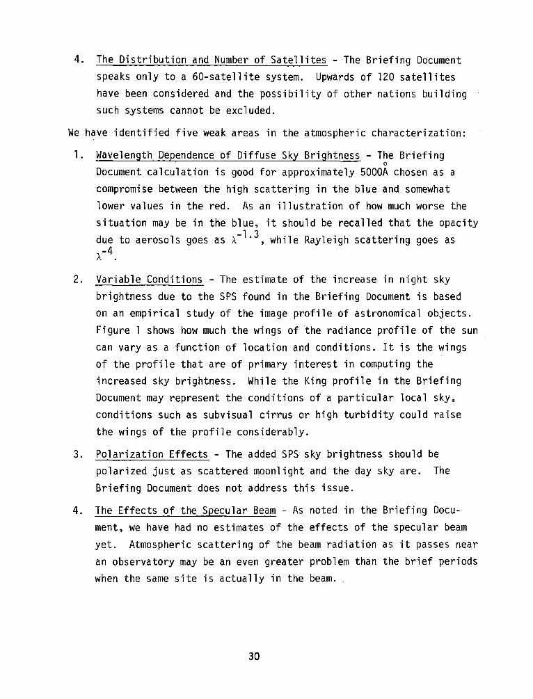
4. The Distribution and Number of Satellites - The Briefing Document speaks only to a 60-satellite system. Upwards of 120 satellites have been considered and the possibility of other nations building such systems cannot be excluded.

We have identified five weak areas in the atmospheric characterization:

1. Wavelength Dependence of Diffuse Sky Brightness - The Briefing 0

Document calculation is good for approximately 5000A chosen as a compromise between the high scattering in the blue and somewhat lower values in the red. As an illustration of how much worse the situation may be in the blue, it should be recalled that the opacity due to aerosols goes as A- 1· 3, while Rayleigh scattering goes as -4 A .

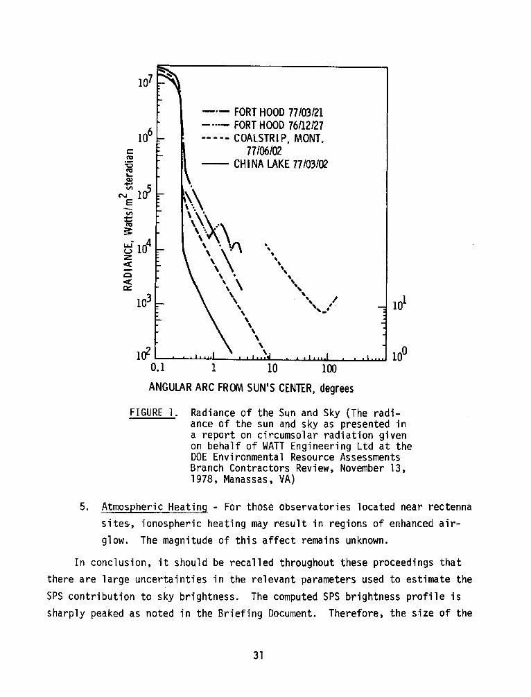
2. Variable Conditions - The estimate of the increase in night sky brightness due to the SPS found in the Briefing Document is based on an empirical study of the image profile of astronomical objects. Figure l shows how much the wings of the radiance profile of the sun can vary as a function of location and conditions. It is the wings of the profile that are of primary interest in computing the increased sky brightness. While the King profile in the Briefing Document may represent the conditions of a particular local sky, conditions such as subvisual cirrus or high turbidity could raise the wings of the profile considerably.

3. Polarization Effects - The added SPS sky brightness should be polarized just as scattered moonlight and the day sky are. The Briefing Document does not address this issue.

4. The Effects of the Specular Beam - As noted in the Briefing Docu­ment, we have had no estimates of the effects of the specular beam yet. Atmospheric scattering of the beam radiation as it passes near an observatory may be an even greater problem than the brief periods when the same site is actually in the beam.

30

c: l'O

"C l'O .... Q)

N~ lrf E -II) = l'O 3:

~-104 z <(

c < a::

-·- FORT HOOD 77 /03121 - ···- FORT HOOD 76/12127 ---·- COALSTRIP, MONT.

77106102 - CH I NA LAKE 77 /03/fll.

1 10 100

ANGULAR ARC FR~ SUN'S CENTER, degrees

FIGURE l. Radiance of the Sun and Sky (The radi­ance of the sun and sky as presented in a report on circumsolar radiation given on behalf of WATT Engineering Ltd at the DOE Environmental Resource Assessments Branch Contractors Review, November 13, 1978, Manassas, VA)

5. Atmospheric Heating - For those observatories located near rectenna sites, ionospheric heating may result in regions of enhanced air­glow. The magnitude of this affect remains unknown.

In conclusion, it should be recalled throughout these proceedings that there are large uncertainties in the relevant parameters used to estimate the SPS contribution to sky brightness. The computed SPS brightness profile is sharply peaked as noted in the Briefing Document. Therefore, the s.ize of the

31

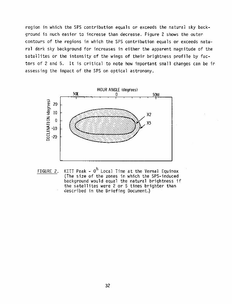
region in which the SPS contribution equals or exceeds the natural sky back­ground is much easier to increase than decrease. Figure 2 shows the outer contours of the regions in which the SPS contribution equals or exceeds natu­ral dark sky background for increases in either the apparent magnitude of the satellites or the intensity of the wings of their brightness profile by fac­tors of 2 and 5. It is critical to note how important small changes can be in assessing the impact of the SPS on optical astronomy.

V'> Q) 20 Q) ..... = Q)

10 "'O

z 0 0 -I-< z -IO _J

~ -20 Cl

5(1: HOUR ANGLE (degrees)

0 sow

X2

FIGURE 2. KITT Peak - Oh Local Time at the Vernal Equinox (The size of the zones in which the SPS-induced background would equal the natural brightness if the satellites were 2 or 5 times brighter than described in the Briefing Document.)

32

COMMENTS ON THE EFFECTS OF INCREASED DIFFUSE SKY BRIGHTNESS ON

FAINT OBJECT ASTRONOMICAL OBSERVATIONS

J. S. Gallagher and S. M. Faber

Progress in astronomy for the last century has been strongly dependent on the development of large telescopes and improved auxiliary instrumentation which have allowed the collection of more information for increasingly fainter objects. For example, the known scale of the universe has increased from that of a single galaxy at the turn of the century to a region of billions of light years containing millions of individual galaxies, primarily through the use of very large telescopes. Based on this history, the astronomical community is committed to building the largest feasible telescopes and equipping them with the best detectors. Even with the advent of space telescopes, large, ground­based telescopes will continue to play a major role in astronomical research during the next 20 years (e.g., the New Generation Telescope program is pur­suing studies of a telescope having an aperture 5 times larger than existing telescopes.)

The sensitivity of even these large instruments is primarily limited by the sky's brightness for observations of faint objects, and any degradation of sky quality is therefore a matter of serious concern. At present, city lights provide the major source of light pollution; astronomers have therefore sought to develop remote sites, such as Mauna Kea in Hawaii, and have encouraged astronomically-oriented cities such as Tucson, Arizona, to pass ordinances designed to curb light pollution. Large artificidl satellites, such as the SPS, pose a new and more ubiquitous problem. When such satellites are illu­minated by the sun, they become bright sources whose light will be scattered in the Earth's atmosphere, thereby increasing the diffuse brightness of the night sky. In addition, direct and scattered light from specularly reflected sunlight could cause a loss of observing time during certain seasons.

For the purposes of a preliminary assessment of the effects of the SPS on

faint-object, ground-based astronomy, we will consider how measurements of the

33

optical light from objects having continuous spectra with absorption lines {galaxies, stars, etc.) and a surface brightness less than the natural night sky depend on the degree of light pollution. Furthermore, as it is difficult to extrapolate astronomical instrumentation over 20 years, we will consider the environmental impact of the SPS on data acquisition using existing techniques.

Two types of detectors are routinely used for studies of faint objects~ photographic emulsions and photon detectors. Photographic emulsions have a large capacity for information storage through the huge number of pixels available, low cost, and acceptable uniformity of response at the expense of linearity and efficiency {quantum efficiencies of at most a few percent). Plates also have the undesirable property that above a threshold, the signal­to-noise ratio for a given area essentially becomes independent of the amount of flux collected. In contrast, photon-counting detectors have higher quantum efficiencies which in principle, though not always in practice, are limited in accuracy only by photon statistics. Detectors of this type provide a best

case for dealing with the problem of sky subtraction.

Now consider an interesting object (star, galaxy, cluster, etc.) which is seen against a natural sky background of surface brightness N photons/cm2

s arcsec2 through some spectral bandpass defined by either a spectrometer or filter. We assume that we are in the optical spectral region and are not centered on a strong night sky emission line; so we will use V band brightness measurements as a representative case. The region of interest within a given object will have a surface brightness gN where often g<<l. We will compare this circumstance with the same measurements taken against a sky with an increased brightness pN (p>l), in which case the object surface brightness is (g/p)pN. The critical question then is how do our observational capabilities

depend on the magnitude of p?

Since the maximum signal-to-noise ratio on a photographic plate over some fixed physical area is set by the emulsion and processing and not by the photon flux, then the detectable signal against sky is always the same frac­tion f of the sky brightness. Thus, under ideal conditions a given plate­telescope combination might allow an intensity level of fN to be recorded,

34

while a polluted sky would increase the recorded intensity to fpN. We might then find losses to be objectionable for p ~ 1.1-1.2 and serious for p > 1.2. Table l provides a description of the sky brightness pattern associated with a full complement of 60 solar power satellites, each having mv = -4.3 and assum­ing a l/r2 diffuse brightness profile under perfect conditions. We take mv =

22 mag arcsec- 2 for the natural sky and consider the brightness in zones centered on the satellites. Table 1 shows that for photographic plates, the SPS-induced background would be serious over approximately 1/6 of the sky and would cover a large fraction (~ 1/4) of the prime region near the meridian. This problem could in principle be overcome by stacking several plates, but systematic errors will probably cause a loss of efficiency so that photo­graphic techniques would no longer be useful over much of the sky. In par­ticular, wide-field survey capabilities with fast Schmidt telescopes would probably become a thing of the past.

TABLE 1. Assumed Sky Brightness Profiles for the SPS (mv = -4.3)

Photographic Photon Counting Loss in: Area {DEC x RA) _£__ Loss in Mag Mag S~eed

30 x 63° 6 1.9 1.0 6

10° x 70° 2 0.75 0.4 2

20° x 75° 1.4 0.4 0.2 1.4

40° x 80° 1.2 0.2 0 .1 1. 2

60° x 90° 1. l o. 1 0.04 1. 1 100 x 70°(a) 4 1. 5 0.75 4

100 x 70°(b) 1.6 0.5 0.3 l. 6

(a) Assumes mv = -5.3 per satellite. (b) Assumes mv = -3.3 per satellite.

35

Photon detectors are affected differently, as it is possible to compen­sate for increased sky brightness by integrating for longer times. The time to reach a given signal-to-noise ratio R over a region of area A arcsec2 with a telescope of collecting area o equipped with a detector of efficiency Q is

Alternatively, the increase in sky brightness decreases the intensity level detectable with a given telescope and fixed integration time by a factor of l//'j) . The variation in ts and the magnitude loss factor for photon counting detectors are also given in Table l, and we see that for an ideal photon detector the SPS background outside of a contaminated zone of 20°x75° is marginally tolerable and is objectionable over 40°x80°. Within this smaller contaminated zone, telescope performance is reduced below an accept­able level.

How will these contaminated areas affect astronomy? Note first that the parallax between will be sufficiently large in declination (10°) such that the contaminated zones for photon detectors overlap in only a small area. Thus, between these two observatory sites, and assuming that by 2000 use of photon detectors will predominate, little of the sky would be irrevocably lost for faint object work. If we take only KPNO and assume that sources will be observed within ±2 hours (±30°) of the meridian, then in principle about 1/6 of the sky will be lost, and studies of objects distributed at random would not be seriously affected. The brightest examples of various astrophysical systems are, however, not distributed at random, and we might well lose access to critical individual objects. For example, the contaminated band as seen from KPNO lies within declinations of +4° to -16°, which includes a selection of very interesting objects such as the bright globular cluster M3, the Orion Nebula, some important galaxies, and several interesting but faint quasars in the equatorial zone. The extra light contributed by the SPS would be detri­mental to frontier optical astronomy.

36

For photographic detectors the situation is, of course, more severe. As seen from KPNO, the contaminated zone extends from declination -28° to +14° and now would include the Virgo cluster, which as the nearest example of a regular cluster of galaxies plays a critical role in extragalactic astronomy

and is a cornerstone in the cosmological distance scale. The contaminated zone also would extend dangerously close to the North Galactic Pole (NGP). In a region around the NGP the blockage due to dust and confusion by galactic stars is at a minimum, and thus the polar regions provide irreplaceable win­

dows within which the large-scale structure of the Universe can be observed.

Thus, if we consider only the diffusely reflected light under ideal conditions, the effects of the SPS are disagreeable for photon detectors and would seriously limit the use of photographic plates or any other detector with finite signal-to-noise ratios. Unfortunately, even at good sites observ­ing conditions are often not ideal. The addition of aerosols or presence of thin clouds, which would produce a minor effect on observations taken against the natural night sky, would increase the level of scattered light. It should be emphasized that even a factor of two increase in the scattered light from SPS would produce an unacceptably large contaminated zone, even for photon

detectors. It therefore is likely that the SPS would lead to a reduction in efficiency due to the loss of imperfect nights for faint object work. Simi­larly, if the brightness of the satellites were to be increased by even a

factor of two over mv = -4.3 (which would occur near midnight for a cosine distribution of reflected light), then even under ideal atmospheric conditions 1/4 or more of the prime observable region would be lost.

There would also be a number of secondary effects. Obviously, the

brightness level of ambient light would increase, necessitating improved shielding and instrument design. In addition, scattered direct light from the

satellites within the telescopes and by the observatory building can produce an additional source of unwanted background light, with the unpleasant poten­

tial for being non-uniform across the telescope's field of view. The back­ground of both direct and scattered light would be time-varying and is, there­

fore, difficult to remove. Finally, scattering processes become more severe

37

at shorter wavelengths, so the SPS background will be more serious at shorter wavelengths (such as the blue and ultraviolet) where most optical data tradi­tionally are obtained.

In conclusion, faint object optical astronomy involves the measurement of weak signals against a comparatively bright, night sky background. It is clear that any additional sources of background light are undesirable and that large structures in space, therefore, can seriously compromise our ability to make optical astronomical observations from the Earth. The SPS sits on the limit of acceptability, and its impact will depend on the details of the design. A 60-satellite system with brigh~ness mv = -4.3 per station would eliminate astronomical 'dark' time (no moon present), which is currently when most faint object astronomy is done. Great care will be required to ensure that we do not lose our observational access to the universe, which would seriously limit the growth of our knowledge of fundamental physical laws, on which techno­logical advances ultimately are based.

38

GENERAL COMMENTS

EFFECTS OF THE SATELLITE POWER SYSTEM ON GROUND-BASED ASTRONOMICAL TELESCOPES

P. B. Boyce

Astronomers are continually working to extract information from the small numbers of photons which arrive at the Earth from distant stars and galaxies. For many years now the brightness of the night sky has been a major limiting factor in the attempt to extend our knowledge of the universe. The blackouts in California during the Second World War provided an opportunity to make some substantial breakthroughs in our understanding of the composition of our neighboring galaxies. We have come a long way since then. We have bigger telescopes at darker sites. We have new detectors with higher efficiencies and better characteristics than the old photographic plates used in the 1940s. We have improved our ability to count photons and detect signals in the pres­ence of the sky background. But the fact remains that the interesting and significant discoveries continue to be made at the limits of what can be detected with the current telescopes, auxiliary instruments and techniques.

For this reason any significant increase in the brightness of the night sky will have a major impact on further progress in astronomy, an impact far­larger than one might think from the small increases in brightness being predicted. The light pollution generated by the SPS will have several unde­sirable characteristics:

1. The additional light will be widespread. Unlike city lights which are confined to relatively limited area, the SPS light pollution will affect all U.S. observatories. A significant number of active foreign observatories will also be affected. Table 1 lists the observatories with telescopes of 1.5-meter-diameter aperture or larger. All the telescopes are in active use and most have been built within the last decade. In particular, the two major foreign

telescopes in Hawaii have just been completed and were placed on

39

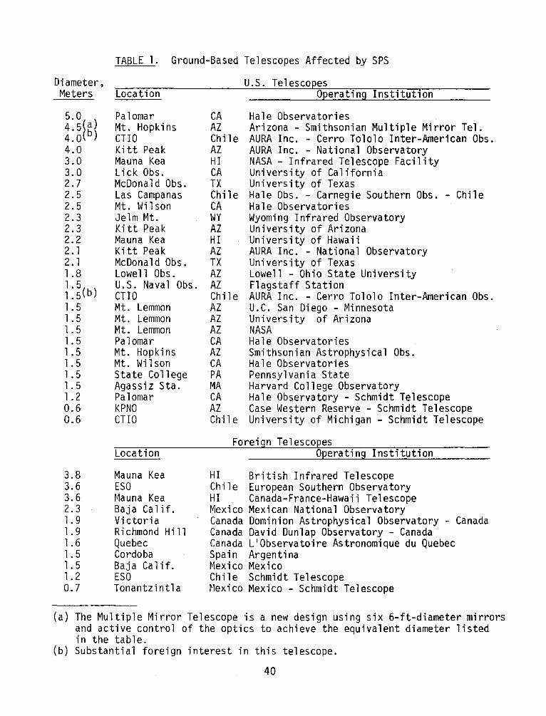
TABLE 1. Ground-Based Telescopes Affected by SPS

Diameter, Meters Location

5.0 4.5~g~ 4.0 4.0 3.0 3.0 2.7 2.5 2.5 2.3 2.3 2.2 2. 1 2. 1 1.8 l. 5( ) l. 5 b l. 5 l. 5 l. 5 l. 5 1. 5 1. 5 1. 5 1. 5 1.2 0.6 0.6

3.8 3.6 3.6 2.3 l. 9 1. 9 1. 6 l. 5 1. 5 l.2 0.7

Palomar Mt. Hopkins CTIO Kitt Peak Mauna Kea Lick Obs. McDonald Obs. Las Campanas Mt. Wilson Jelm Mt. Kitt Peak Mauna Kea Kitt Peak McDonald Obs. Lowell Obs. U.S. Naval Obs. CTIO Mt. Lemmon Mt. Lemmon Mt. Lemmon Palomar Mt. Hopkins Mt. Wilson State College Agassiz Sta. Palomar KPNO CTIO

Location

Mauna Kea ESQ Mauna Kea Baja Calif. Victoria Richmond Hill Quebec Cordoba Baja Ca 1 if. ESQ Tonantzintla

CA AZ Chile AZ HI CA TX Chile CA WY AZ HI AZ TX AZ AZ Chile AZ AZ AZ CA AZ CA PA MA CA AZ Chile

U.S. Telescopes Operating Institution

Hale Observatories Arizona - Smithsonian Multiple Mirror Tel. AURA Inc. - Cerro Tololo Inter-American Obs. AURA Inc. - National Observatory NASA - Infrared Telescope Facility University of California University of Texas Hale Obs. - Carnegie Southern Obs. - Chile Hale Observatories Wyoming Infrared Observatory University of Arizona University of Hawaii AURA Inc. - National Observatory University of Texas Lowell - Ohio State University Flagstaff Station AURA Inc. - Cerro Tololo Inter-American Obs. U.C. San Diego - Minnesota University of Arizona NASA Hale Observatories Smithsonian Astrophysical Obs. Hale Observatories Pennsylvania State Harvard College Observatory Hale Observatory - Schmidt Telescope Case Western Reserve - Schmidt Telescope University of Michigan - Schmidt Telescope

Foreign Telescopes Operating Institution

HI British Infrared Telescope Chile European Southern Observatory HI Canada-France-Hawaii Telescope Mexico Mexican National Observatory Canada Dominion Astrophysical Observatory - Canada Canada David Dunlap Observatory - Canada Canada L'Observatoire Astronomique du Quebec Spain Argentina Mexico Mexico Chile Schmidt Telescope Mexico Mexico - Schmidt Telescope

(a) The Multiple Mirror Telescope is a new design using six 6-ft-diameter mirrors and active control of the optics to achieve the equivalent diameter listed in the table.

(b) Substantial foreign interest in this telescope.

40

Mauna Kea after an exhaustive search for the darkest and best sites in the world. The reaction of the respective governments to the SPS will have to be considered.

2. The scattered light will have the spectrum of sunlight. Compensat­ing for such a spectrally complex background will be more difficult than correcting for light scattered from incandescent street lamps. In comparison to low-pressure sodium and mercury vapor lamps, the situation is even worse. They emit much of the light in a few spectral lines, leaving the space in between relatively uncontam­inated. The SPS light will contaminate the whole observable spectral range. The scattered light will be polarized and will vary with time because of varying concentrations of dust and aerosol in the atmosphere.

3. At certain times the specular reflection from the satellites could pose a danger to astronomers' eyes and to instruments. While this possibility is remote, it will have to be guarded against and will require the installation of special TV camera systems at all tele­scope eyepieces. It is not clear how to protect amateur astrono­mers, sailors and general sky watchers who use telescopes or . binoculars.

4. The string of satellites located along the equator will completely block out access to the Orion Nebula for optical and infrared tele­scopes in the U.S. As the closest large region of star formation, the Orion Nebula plays a key role in helping to clarify how stars and planetary systems are fanned and the process by which material, after being incorporated into stars, is once again recycled into the interstellar medium. The SPS zone of avoidance will be invariant with time, pennanently denying U.S. astronomers access to an impor­tant section of our galaxy, including parts of the galactic spiral arms just interior to our own. Studies which depend on completeness in order to develop a coherent picture of our own galaxy will no longer be possible.

41

SPECIFIC COMMENTS

The effects of increased sky brightness on astronomical measurements have been well treated elsewhere in this workshop. Effects may slightly vary depending on the type of detector and telescope. For example, photographic film is much more sensitive to increasing sky background than is a linear detector with a large storage capacity. But it is cl~ar that we will have to rely on photographic film as a simple yet effective detector for large format­imaging applications for some time to come.

For a linear, photon-counting detector the limitation is the sky back~

ground. Most of the significant work being done in optical astronomy now involves observing objects at levels between 1/10 and 1/100 of the sky back­ground. At these levels the effective observing time needed to achieve a given

accuracy with a given telescope scales linearly with the increase of sky background. However, beyond an exposure time of several minutes, the stabil­ity of instrumentation and observing conditions becomes a negative factor.

It is impossible to express this rigorously, but the effective limit to expo­sure time is about one hour.

Some of the assumptions used in preparing the Briefing Document for the workshop do not appear to be valid, specifically:

l. The light scattered back into the atmosphere should not be ignored in computing the increase of sky brightness. This will be variable in time and place. In winter with a snow blanket the present mea­sured sky brightness at places such as Lowell Observatory increases markedly. For Mauna Kea, which is surrounded by a high albedo ocean, the backscattering must be significant. It will be difficult

to estimate, but some attempt should be made.

2. The assumption of 4% reflectivity for the concentrator configuration is not valid. The configuration will act as a corner cube (within certain limits) and will effectively reflect from the whole area.

From half the area the angle of reflection off the sapphire cover

will be 30°, which should increase the reflectivity. I would expect the total reflectivity to be closer to 8%.

42

3. The far (> 1°) wings of the scattering profile assumed for this study have not been measured well to my knowledge. It is not clear

that the l/r2 profile is anything more than a best guess at this

point. The scattering will be critically sensitive to dust and aerosols in the atmosphere.

NEW INSTRUMENTS

Astronomy is in the midst of a period of tremendous intellectual growth and excitement. This has been fueled in part by the improvement in instru­mentation used to overcome physical limitations. The number of major tele­scopes at good, dark-sky sites has more than tripled in the last decade. It is no accident that most of these new telescopes, whether U.S. or foreign, were built along the west coasts of North and South America and on Hawaii. These sites are the premier astronomical sites in the world. Unfortunately, they lie directly under the SPS array.

Astronomers, always faced with the photon limit, are now considering a

new type of telescope which will provide much larger apertures of 10 to 25 meters. The University of California is planning for the construction of a 10-meter instrument which would be located in California and would serve the entire University of California system. The Kitt Peak National Observatory

has also started on a program which will lead to the construction of a 25-meter telescope. Both these instruments are being built to observe faint and dis­tant objects, fainter by far than can be reached by the space telescope (which is only a 100-inch telescope). They would operate in the regime where increas­ing sky brightness would be most detrimental.

Unfortunately, new detectors are not the answer. For many applications the technology .is already available to record and count all possible photons and to subtract the contribution from the sky as effectively as possible. The

next generation of optical telescopes will suffer the full brunt of any increased sky brightness, losing capability linearly with increasing bright­ness and being effectively blocked from access to an interesting portion of

the sky.

43

INFRARED ASTRONOMY

D. A. Harper

In general, the impacts of the SPS on infrared (IR) observations should be much less severe than on optical measurements. For example, many infrared telescopes can be operated quite successfully during the daytime. Daytime operations are typically limited by the absolute pointing of the telescope or atmospheric turbulence rather than by increased sky background.

However, IR telescopes are usually designed to minimize the total ther­mal background from the telescope itself, a requirement which is often incom­patible with effective baffling of stray light. Thus, a problem may arise if a very bright object such as the SPS satellite array is located within a few degrees of a faint infrared source. The magnitude of the problem will depend on the design of individual telescopes and the nature of the desired observa­tions. However, it is probably reasonable to assume that an array of 60 sat­ellites, each representing a 330°K radiator with a projected area of~ l square arcminute, will compromise observations of very faint objects within a strip of sky no larger than ~ 2 to 10° wide and 60° long.

45

POSSIBLE IMPACTS OF THE SPS ON THE SPACE TELESCOPE

E. J. Groth

The goals of the Space Telescope (ST) as described in the NASA Announce­ment of Opportunity are to determine:

• The constitution, physical characteristics, and dynamics of celestial entities

• The nature of processes which occur in the extreme physical conditions existing in and between astronomical objects

• The history and evolution of the universe

• Whether the laws of nature are universal in the space-time continuum.

To meet these goals, the ST must be able to detect and measure objects which are several magnitudes fainter than can be observed with ground-based telescopes.

The main advantage of the ST is that its 2.4-m aperture produces diffrac­tion limited images; therefore, the background light within a stellar image is reduced several orders of magnitude compared to what can be obtained on the ground. Other advantages of the ST are that it can work in the UV and IR spectral regions; there is no atmospheric absorption and emission or fluctua­tions in the absorption and emission; and the image size is smaller than 0.1 arcsec (as compared to> 1 arcsec from the ground), which not only increases the S/N for stellar objects by a factor of >20 compared to an identical ground­based telescope but also allows high resolution studies of extended objects.

The orbit of the ST is circular and at an altitude of 500 km, an incli­nation of 28.8° and with a period of 94.5 minutes.

The background sources which limit the sensitivity of the ST are:

• Zodiacal light (23 mv/arcsec2 at minimum)

• Stray light from Sun, Earth, and Moon (and'SPS).

The zodiacal light (sunlight scattered from interplanetary dust particles) is a diffuse source with a minimum brightness corresponding to about 23 visual

47

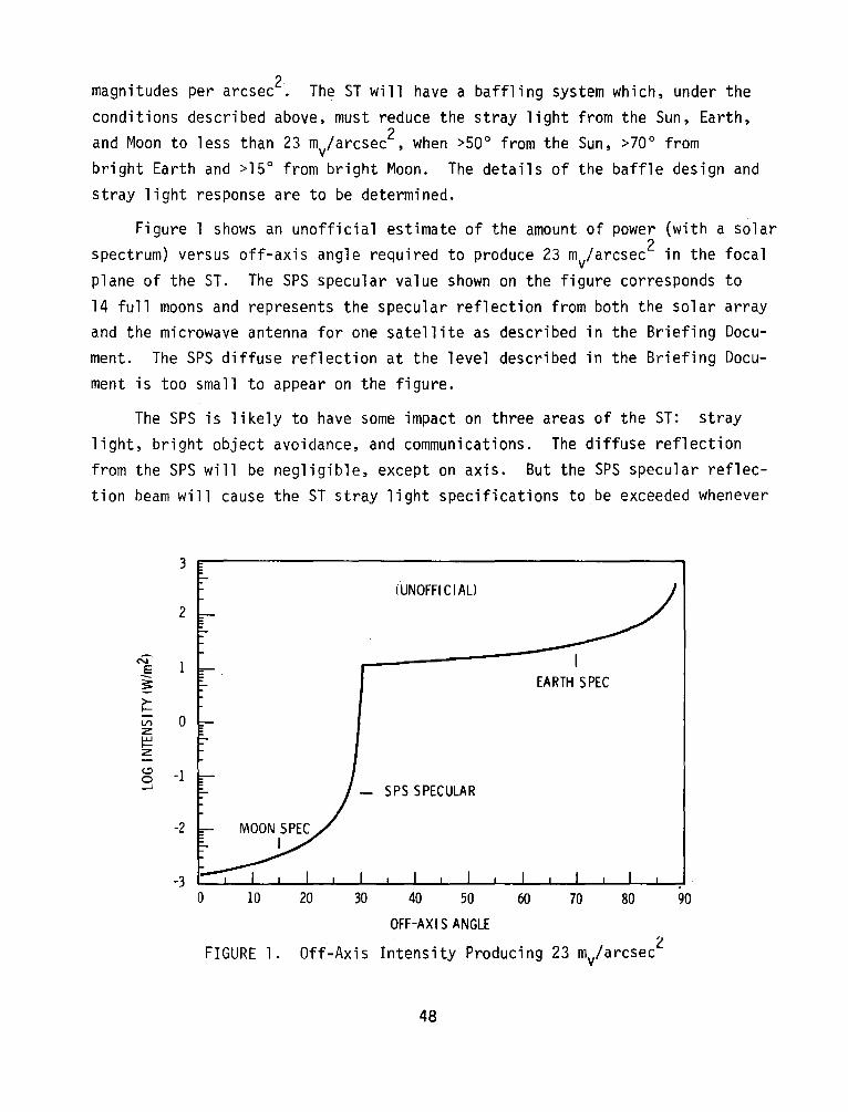
2 magnitudes per arcsec . The ST will have a baffling system which, under the conditions described above, must reduce the stray light from the Sun, Earth, and Moon to less than 23 mv/arcsec2, when >50° from the Sun, >70° from bright Earth and >15° from bright Moon. The details of the baffle design and stray light response are to be determined.

Figure 1 shows an unofficial estimate of the amount of power (with a solar spectrum) versus off-axis angle required to produce 23 mv/arcsec2 in the focal plane of the ST. The SPS specular value shown on the figure corresponds to 14 full moons and represents the specular reflection from both the solar array and the microwave antenna for one satellite as described in the Briefing Docu­ment. The SPS diffuse reflection at the level described in the Briefing Docu­ment is too small to appear on the figure.

The SPS is likely to have some impact on three areas of the ST: stray light, bright object avoidance, and communications. The diffuse reflection from the SPS will be negligible, except on axis. But the SPS specular reflec­tion beam will cause the ST stray light specifications to be exceeded whenever

3

2

N' E ~ >-I-

V'l 0 z I== z (.!) -1 0 _..J

-2

-3 0 10

FIGURE l.

(UNOFFICIAL)

EARTH SPEC

- SPS SPECULAR

20 30 40 50 60 70 80

OFF-AXIS ANGLE 2

Off-Axis Intensity Producing 23 mv/arcsec

48

90

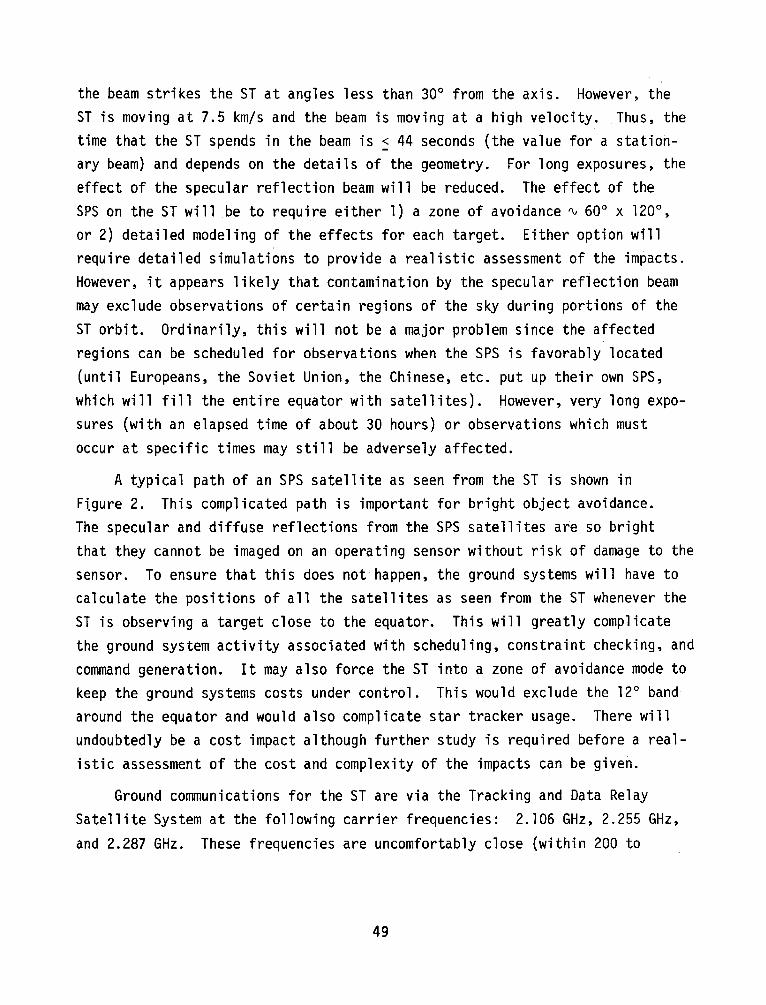
the beam strikes the ST at angles less than 30° from the axis. However, the ST is moving at 7.5 km/s and the beam is moving at a high velocity. Thus, the time that the ST spends in the beam is ~ 44 seconds (the value for a station­ary beam) and depends on the details of the geometry. For long exposures, the effect of the specular reflection beam will be reduced. The effect of the SPS on the ST will be to require either 1) a zone of avoidance~ 60° x 120°, or 2) detailed modeling of the effects for each target. Either option will require detailed simulations to provide a realistic assessment of the impacts. However, it appears likely that contamination by the specular reflection beam may exclude observations of certain regions of the sky during portions of the ST orbit. Ordinarily, this will not be a major problem since the affected regions can be scheduled for observations when the SPS is favorably located (until Europeans, the Soviet Union, the Chinese, etc. put up their own SPS, which will fill the entire equator with satellites). However, very long expo­sures (with an elapsed time of about 30 hours) or observations which must occur at specific times may still be adversely affected.

A typical path of an SPS satellite as seen from the ST is shown in Ftgure 2. This complicated path is important for bright object avoidance. The specular and diffuse reflections from the SPS satellites are so bright that they cannot be imaged on an operating sensor without risk of damage to the sensor. To ensure that this does not happen, the ground systems will have to calculate the positions of all the satellites as seen from the ST whenever the ST is observing a target close to the equator. This will greatly complicate the ground system activity associated with scheduling, constraint checking, and command generation. It may also force the ST into a zone of avoidance mode to keep the ground systems costs under control. This would exclude the 12° band around the equator and would also complicate star tracker usage. There will undoubtedly be a cost impact although further study is required before a real­istic assessment of the cost and complexity of the impacts can be given.

Ground communications for the ST are via the Tracking and Data Relay Satellite System at the following carrier frequencies: 2. 106 GHz, 2.255 GHz, and 2.287 GHz. These frequencies are uncomfortably close (within 200 to

49

FIGURE 2. Typical One-Day Path of SPS as Seen from ST

300 MHz) to the SPS microwave transmission frequency (2.45 GHz). Further study is required to determine whether communications with the ST will be adversely affected by the SPS.

To summarize, the scientific performance of the ST will be somewhat affected by stray light from the SPS specular reflection beam; the need to avoid imaging both the diffuse and specular reflections from the SPS will lead to adverse cost, complexity, and flexibility impacts; and there is a possibility that the ST communication links will be affected by interference from SPS microwave transmissions. In all cases, further study is required to fully define the nature and extent of the possible impacts identified here.

50

REPORT OF THE OPTICAL ASTROMONY WORKING GROUP

REPORT OF THE OPTICAL ASTRONOMY WORKING GROUP

The optical astronomy working group met in order to synthesize the con­tents of the Briefing Document and the invited presentations into a statement of the potential impact of the SPS on optical astronomy. In the judgment of the working group. the primary effect of the SPS on optical astronomy (an effect that could be properly characterized from the description of the Reference System) would be through the predicted increases in brightness of the night sky, as described in the briefing document. For this reason, the working group's deliberations focused on the effect on optical astronomy of the diffuse reflections from the satellites. Other concerns, such as the effects of the specular beam and possible impacts on infrared and space astronomy, are not treated in detail, primarily because 1) understanding of potential SPS effects is inadequate, as in the case of airglow from an SPS­heated ionosphere, and 2) the details of other effects could only be completely characterized if more specific information were available about the Reference System. For example, specific effects of specular reflections from the antenna depend heavily on rectenna siting and antenna properties.

The report of the working group that follows is based on an outline and some text developed by the working group members during the two-day workshop. Most of the report writing was delegated to the chairman of the session, with the understanding that the working group would have the opportunity to review it prior to publication. The report consists of five parts: 1) an introduc­tion to the way in which astronomical observations are performed, which is intended to provide background to readers unfamiliar with astronomical problems and techniques; 2) a discussion of the way in which the Reference System would impact astronomy if it were built, 3) a quantitative discussion of the magnitude of SPS effects and their relationship to astronomical observa­tions, emphasizing the relative magnitudes of natural and SPS-induced sky brightness; 4) the working group's assessment of the qualitative impact of SPS on optical astronomy; and 5) a set of recommendations for future study of SPS effects on optical astronomy and a disucssion of possible methods of miti­

gating these effects.

53

The members of the working group were:

B. Balick P. Boyce K. Clark J. Gallagher E. Groth o. Harper G. Stokes, Chairman

THE NATURE OF ASTRONOMICAL OBSERVATIONS

Counting Photons

The actual method of conducting astronomical research is the root of any effect of the proposed SPS on astronomy, and on optical astronomy in parti­cular. Astronomy is an observational rather than an experimental science. Although laboratory measurements of the properties of matter are extremely important to astronomy, the success of astronomical research is measured largely by its ability to explain objects and phenomena over which we have no control. Astronomy is the extreme case of remote sensing. The information we have about astronomical objects comes almost entirely from our ability to detect the electromagnetic radiation emitted, reflected or affected by the astronomical objects.

As noted in the introduction to these proceedings, astronomy is sometjmes divided according to the portion of the electromagnetic spectrum under study. An important characteristic of optical astronomy is its preoccupation with the detection of photons.

A photon can be thought of as a packet of light. A photon of visible light represents about 4 x lo- 12 ergs of energy, which means that if a 100-watt light bulb emitted 100 watts of visible photons, it would emit 1020 of them every second. Detectors used in optical astronomy are sensitive enough to detect single photons. In many cases, astronomical detectors are merely photon counters.

54

An important problem encountered in photon counting is that the answer arrived at includes an uncertainty corresponding to the square root of the total number of photons counted. Therefore, the fractional error in the number of photons detected is l/~ where N is the total number of photons detected. If an astronomer counts 100 photons, the uncertainty is 10%, if 10,000, the uncertainty is 1%.

Unfortunately, the detection of photons from astronomical objects is complicated by the fact that the sky is a source of photons as well. In the case of an idealized astronomical observation, one can imagine looking at an astronomical object with a typical optical detection system and trying to make an observation with 1% accuracy. Because the detector cannot avoid looking at both the sky and the object, it collects and counts the photons from both. However, when the object is very much brighter than the sky, the photons from the sky make a negligible contribution to the total signal, and we get 1% accuracy just as soon as we have detected 10,000 photons from the source. In such a case, the brightness of the source determines how long the observation will take. If, however, the.number of photons received from the sky is comparable to or greater than the number from the object under study, then the brightness of a nearby portion of sky must be determined and sub­tracted from the observation of the object. However, sky photons can only be measured at best to an accuracy of l/~ just as photons are from the object. For example, if the sky is nine times brighter than the object and our detector counts 10,000 photons from the sky and object together, which gave us 1% accuracy before, our accuracy for measurement of the object would only be 10%. In this case, the observation is said to be 11 sky limited 11 --in order to get a 1% measurement of our source, the detector must have detected 1,000,000 photons. This value represents 100,000 photons from the source or ten times as many as was required to get a 1% measurement without the sky. Therefore, even if the sources in our two examples were the same brightness, the addition of the bright sky would increase by a factor of ten the amount of observing time required for the same accuracy measurement.

55

It is exactly these considerations that led to Gallagher and Faber's equation (see their invited paper) that gives the amount of time necessary to reach a given signal-to-noise ratio (fractional error),

( l )

In this equation, g is the ratio of the brightness of the object to the brightness of tj'le natural sky, p is the ratio of the actual sky brightness to the natural sky brightness (p always ~ 1), R is the desired signal-to-noise ratio, Ax N is the brightness of natural sky in photons/sec/cm2 , Q is the detector efficiency and o is the collecting area of the telescope in cm2. For the case of faint objects:

2 t = p x l x _2_R -s o g2AQN

(2)

which means that required observing time is proportional to the brightness of the sky and inversely proportional to the collecting area of the telescope. It is easy, then, to understand why astronomers need dark skies and large telescopes to observe faint objects.

Astronomical Accommodation to Existing Sources of Sky Brightness

Natural and man-made sources of sky brightness already have a significant impact on the conduct of optical astronomy. The largest natural contribution to the diffuse night sky brightness comes from the moon. The moon has such a profound effect on the sky that observatories routinely divide their observing schedule into 11 dark11 (no moon) and 11 bright 11 (moon up) time. Generally, dark time is in much greater demand than bright time on large telescopes, as seen in the distribution of visitor proposals at Kitt Peak National Observatory (KPNO) for dark time and bright time for February 1, 1979 to July 31, 1979 (Table 1).

56

TABLE 1. Visitor Proposals for Time on the Three Largest Telescopes at KPNO February 1, 1979 to July 31, 1979

Telescope

4.0 meter

Dark Bright

2. 1 meter

Dark Bright

1.3 meter

Dark Bright

Number of Nights Requested by Visitors

184

117

181

92

130

98

Number of Nights Available for

Visitor Observing

47 49

44 41

49

49

At present, the primary man-made source of sky brightness is outdoor light from cities and towns. Astronomers have attempted to combat this light pollution in a number of ways-the most obvious, building telescopes in remote locations well away from city lights. For example, the detailed site surveys that precede construction of a major observatory always include assessments of the sky brightness. In some cases, urban areas have grown up adjacent to observatories. At some of these observatories, observations are limited to the kinds of of objects observed during 11 bright 11 observing time at darker sites as is the case at Mt. Wilson Observatory where the light pollution from Los Angeles and nearby cities makes the sky very bright. At other observa­tories, observatory staffs have attempted to convince local public officials that it is possible to control light pollution and minimize the effects of outdoor lighting on astronomy. Tucson, Arizona and Richland, Washington, among others, have very strong light abatement ordinances specifically tailored to

preserve dark skies.

57

Astronomical Observations: Types of Objects

It is now appropriate to consider the kinds of objects most sensitive to increased sky brightness. Objects of astronomical observations fall into two categories: point sources and extended sources. Returning to equation (1), we note the term A x N, the brightness of the sky. This brightness is a product of N, the number of photons coming from a unit of area of the sky, and A, the amount of sky being observed. For point sources, every attempt usually is made to make A as small as possible. Although there are limits as a result of the turbulence of the atmosphere, a small aperture does repre­sent a practical method of reducing the effect of sky brightness for objects that appear as point sources, such as stars.

However, this strategy will not work for extended objects, such as galaxies. In order to reduce the amount of sky being observed, one must correspondingly reduce the amount of the object to be studied. The case of galaxies is an important one since the average surface brightness of a galaxy (the number of photons emitted per unit area) is considerably less than the average brightness of the dark night sky. Galaxies are brighter toward their nuclei; therefore, the net effect of increasing the sky brightness is to reduce the amount of a galaxy that can be observed. This effect is qualita­

tively illustrated in Figure 1. The research consequences of not being able to observe the outer regions of galaxies are noted, along with other research programs, after the following section.

Astronomical Observations: Organization and Conduct of Programs

An observing program is the set of observations that astronomers will make in order to address a particular astronomical problem. The organization of typical observing programs is important because the increase in diffuse sky brightness as a result of SPS is a function of position on the sky, which implies that in particular regions of the sky it will not be possible to observe particular kinds of objects.

Observing programs consist of surveys and type studies. Most observing

programs include elements of both kinds of studies. A survey entails the

58

• •

• •

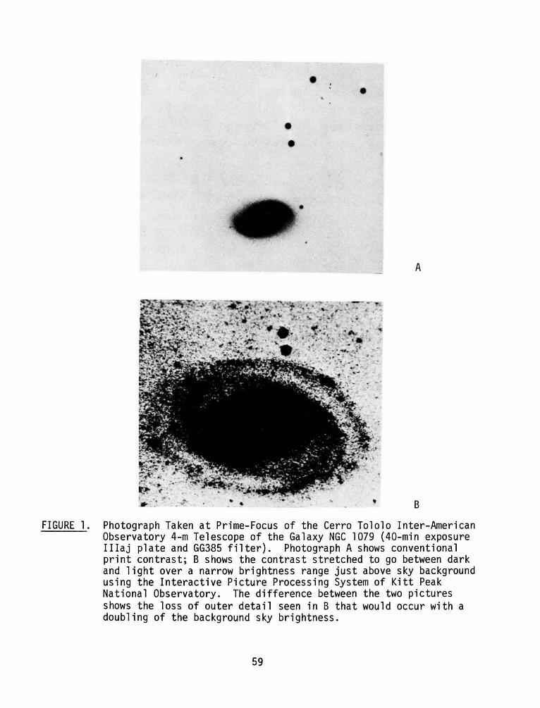
A

B

FIGURE 1. Photograph Taken at Prime-Focus of the Cerro Tololo Inter-American Observatory 4-m Telescope of the Galaxy NGC 1079 (40-min exposure Illaj plate and GG385 filter). Photograph A shows conventional print contrast; B shows the contrast stretched to go between dark and light over a narrow brightness range just above sky background using the Interactive Picture Processing System of Kitt Peak National Observatory. The difference between the two pictures shows the loss of outer detail seen in B that would occur with a doubling of the background sky brightness.

59

measurement of a few parameters for a large number of objects. An example is

the National Geographic-Palomar Sky Survey. This survey, conducted in the 1950s, consists of photographs taken through two different colored filters of

• almost the entire sky visible from Mt. Palomar. A type study is the detailed study of a single object that is either unique pr thought to be representative of a class of objects. Generally, type examples are usually the nearest members of the class.

When planning the details of an astronomical observing program--specifi­cally, what objects are to be observed--several other factors must be considered. The most important is the fact that the atmosphere is not completely trans­parent so that the flux of photons from an object is attenuated as it passes through the atmosphere. The amount of attenuation is exponentially related to the amount of the atmosphere the radiation passes through, which is mea­sured in airmasses. An airmass is the ratio of the amount of air toward the object to the amount of air toward the zenith, the point straight above the observer. In order to maximize the number of photons observed, observations must be planned to minimize the average airmass through which the object is observed. ln practical terms, this usually means that an object will be observed during the time that the object is within 30° of the meridian, an imaginary line on the sky on which astronomical objects are at their minimum airmasses. Objects are in this band for four hours every day. Many astrono­mers have concluded that four hours is a practical upper limit for a single observation.

Finally, because objects more than 60° from the zenith must be observed through more than two airmasses, objects that never come closer than 60° to the zenith are usually not included in an observing program.

Astronomical Observations: Scientific Programs

Listed here are current areas of active research that would be negatively affected by the SPS program. These research areas are typical, but no effort at completeness is intended.

60

Cosmolo and Extra alactic Astronom Studies of Ob"ects Be ond the Milky Way

Distances to extragalactic objects are very great. For this reason, most galaxies, although as luminous as several billion stars, are as difficult to discern and study as the faintest stars visible in our own galaxy.

1) The Size of the Universe. Measurements of the size of the universe depend on our ability not only to observe the most distant (and faint) objects but also to develop techniques for distance measurement. The identification of distant objects is extremely marginal because of their faintness and is complicated by the presence of a bright sky background 11 against 11 which they must be viewed from the ground. Even small increases in sky brightness can render these objects undetectable.

2) Curvature of the Universe. Ever since its beginning 15 billion years ago, our expanding universe has probably been decelerating as the attractive gravitational forces between all massive objects operate to counteract the initial expansion. This deceleration, however, is not large at the present time. At an earlier epoch, objects were closer together and the effects of gravity were stronger. The finite speed of light affords us an opportunity to study the ancient universe--but only at distances of ~15 billion light-years. A question of nearly universal interest is the ultimate fate of our universe: will it ever fall back on itself (closed), or will it expand forever (open)? The answer will come directly from measuring the deceleration of the universe.

3) Formation Era of Galaxies. All galaxies are believed to have formed as soon as the early universe cooled to a few thousand degrees (some 100,000 year~ after the big bang) but before the expansion of the universe spread the available matter over large distances. The formation of galaxies is extremely complex, and our comprehension of existing galaxies is incomplete without a good idea of the initial conditions of formation.

4) Open or Closed Universe? In addition to the difficult observational strategy of measuring the deceleration of the universe, the question of

an open or closed universe can be settled by measuring all of the mass in the universe. At present, the visible forms of mass accessible to

61

observation (luminous stars and heated dust and gas) fall far short of the critical mass required for closure. Many recent studies, both theoretical and observational, indirectly suggest that more mass might exist, perhaps in extremely faint halos around galaxies. Attempts to observe faint galactic halos are suggestive, but limited by the sky background.

5) Active Galaxies and Quasars. Events leading to and the effects of the tremendously large energy sources in the centers of exploding galaxies and quasars have captivated the interests of both astronomers and the public for nearly a generation. Although the nuclei of these objects are often bright, the material ejected into space and the processes that supply energy to the nuclei are very faint and difficult to observe.

6) Faint Regions of Nearby Galaxies. Nearby galaxies afford favorable observing opportunities because of their proximity, and intense efforts to understand their structure and evolution have characterized modern astronomy. T,hese faint regions not only may contain the mass necessary to close the universe but also reflect the subtle tidal effects that galaxies exert on each other.

The Milky Way.

Our galaxy is one of the most interesting, yet enigmatic, of astronomical objects. We look to our solar neighborhood to understand how stars are born, live their lives, and die, and to understand how our galaxy is structured. The nuclei of many galaxies harbor unusual and, as yet, not understood energetic processes. What about our own? Do other stars have planets? To complicate observations, large clouds of dust hide 90% of the galaxy from view to observers using optical and ultraviolet techniques. The effective size of the visible galaxy would be severely diminished by even small increases in the night sky levels.

1) Diffuse Galactic Light. 11 Hot tunnels 11 carved through the galaxy by supernova blast waves appear to permeate the galaxy. Many studies are

underway to understand the physical conditions (e.g., temperatures of a

62

million degrees) through optical and ultraviolet observations, but the light levels from these regions are very, very low (they were only recently discovered).

2) Faint Nebulae. The following are all types of objects which have been of intense interest to astronomers for the past century: the remnants of supernova explosions (once the interior of stars); material ejected from thermonuclear detonations on the surfaces of white dwarfs; material lifted off the surface of a dying star by its own light and acoustic noise; and material ionized by energetic photons of very hot stars. Not all of these objects are faint, but most of the interesting ones have important properties that require low background levels in order to be studied.

3) Stellar Winds and Mass Loss. Stars are formed from the reservoir of dust and gas in our galaxy. It is easy to show that this reservoir is being depleted at a rate so large that, without replenishment, star formation would be completely arrested in only a billion years (the galaxy is thought to be many billions of years old). It seems certain that replen­ishment occurs, but it is not clear how. Recent studies have shown that many stars continuously lose their mass through a stellar "wind." Studies of the very faint wind and how the material in the wind finds it way back into the interstellar reservoir are at the limit of modern techniques.

4) Structure of the Galaxy. We now understand the galaxy to consist of spiral arms of gas, dust, and young stars. Outside and between the spiral arms, the structure of our galaxy is poorly understood--partly because the stellar constituents are cool and faint for the most part. Even though billions of stars are involved, their light and problems of foreground dust make studies of these objects very difficult. Studies of stars outside the galaxy in a surrounding "halo'' and in extremely old "globular" clusters that appear to have been formed at about the same time as the galaxy are important to our understanding the general

problem of galaxy formation and evolution.

63

The Solar System.

We need not describe here the interest of the public as well as of the scientific community that has been raised by studies of objects in the solar system; indeed, the magnitude of NASA programs in this area speaks for itself. The planets themselves, while of prime interest, are generally very bright, and ground-based studies of them and their satellites would not be greatly affected by SPS light pollution. There are, however, other interests in the solar system for which a bright background would severely impede ground-based research.

For example, comets and their tails, asteroids, and other "minor" con­stituents of the solar system are generally faint. The plane of the ecliptic is fairly closely aligned with the equatorial plane of the Earth and the satellites, and the faint objects found preferentially in the ecliptic plane, such as minor bodies, will be difficult to observe near the satellites. Although comets do not have ecliptic orbits, they and their tails are generally in their most favorable aspects as they near the ecliptic. Similarly, the zodiacal light is also confined to the ecliptic plane and, likewise, will be difficult to observe near the satellites.

THE ORIGIN OF SPS EFFECTS ON OPTICAL ASTRONOMY

The single most important point to keep in mind when considering the effects of SPS on optical astronomy and aeronomy is that the major effect, the increase of sky brightness, stems from the passive properties of the system. As such, this effect is inherent in any space-based power collection scheme. For the Reference System, the solar blanket intercepts 70 GW of solar radiation, only 6 GW of which is actually radiated toward Earth in the microwave beam. The most important portion of the remaining 64 GW of energy which has an effect on astronomy is the light reflected from the front surface of the blanket. This reflected radiation constitutes approximately 7 to 15% of the visible radiation incident on the solar blanket and is made up of both diffuse and specular reflection, as described in the Briefing Document. The diffuse

reflection is responsible for the most persistent and troublesome effects on

64

astronomical and aeronomical observations. The magnitude of the effects is determined by the apparent brightness of the satellites and the properties of the atmosphere. In turn, the brightness of the satellites is determined by their size and reflectivity. The satellites will be exceeded in brightness by only the sun and the moon. Each one will in fact be bright enough to cast a shadow.

Parametric Characterization of the Effect of the SPS on Diffuse Sky Brightness

In order to meaningfully assess the SPS effects on diffuse sky brightness, the computations presented in the Briefing Document and the limitations of the Briefing Document as discussed in the invited presentation of G. M. Stokes were carefully considered. While the working group·ag~eed that the SPS effects can all be described in terms of the apparent brightness of the satellites, the useful numbers for designers of the power satellites are the collecting area and the reflectivity of the various parts of the satellites.

The problem of a large collecting area is not solved simply by reducing satellite size. The important number is the total collecting area for the system, which for the Reference System is 3300 km2, about the size of the state of Rhode Island. A reduction in total surface area would require an increase in the overall efficiency of the System, whtch is now about 7%. Analysis in the Reference System documentation does not suggest that the overall efficiency of the SPS will change much. If this is the case, then the most important parameter in determining the apparent brightness of the satel­lite is its albedo, which is the ratio of the radiation reflected from an object to the total incident radiation. As noted in the preceding section, the albedo consists of a specular component, a measure of the extent to which the object acts like a mirror, and a diffuse component, which is a measure of one's ability to see the object in any aspect.

The working group's deliberations on the diffuse albedo of the SPS solar blankets led to two conclusions. First, the diffuse albedo of 4%, as des­cribed in the Briefing Document, is an optimistic estimate. As such, the effects predicted on the basis of the 4% albedo were taken as lower limits of the possible effects of the SPS on optical astronomy. A second, related

65

conclusion, was that the relative distribution of reflected radiation between the diffuse and specular components of an actual SPS was likely to be quite

different than the 50-50 distribution assumed in the Briefing Document. In particular, the potential hazard to eyesight that the specular reflections may represent will undoubtedly lead to designs specifically tailored to reduce the energy contained in the specular beam. In the opinion of the working group, the most likely solutions to the problem of the specular beam will result in an increase in the diffuse albedo, and the reduction of the total albedo of the individual satellites (diffuse albedo plus specular albedo) is not likely. The solutions will rather be of the kind that make the antenna structure and solar blanket less like a mirror and more like a piece of white paper. Given the optimistic estimate of the diffuse albedo and the likely fate of the large specular reflections, it would not be surprising if the actual diffuse albedo of the satellites reached 10%, two and a half times the Briefing Document estimate.

In summary, it was the concensus of the working group that the magnitude of diffuse albedo of the individual satellites is the major factor in deter­mining the effect of the reference SPS on optical astronomy.

Intensity Profile of the.SPS Brightness Distribution

An essential feature of the Briefing Document is that it attempts to provide a method for calculating the distribution of added sky brightness as a res,ult of the SPS. There are limits to the practicality of this approach as described by Stokes in his discussion of the limitations of the Briefing Document characterization. In spite of the fact that the actual brightness distribution around an individual power satellite will depend strongly on physical conditions, several properties of the brightness distribution of the entire system are relatively independent of local physical co~ditions.

As described in the Briefing Document, the area of increased brightness

is sharply peaked. In Figure 2 the predicted increase in the sky brightness along the meridian at midnight for Kitt Peak National Observatory has been plotted for a 60-satellite system. While the intensity scale shown in the figure is for a satellite brightness equal to that of Venus, the shape of the

66

18 (_) a::: ~ u.. 0 Cl 20 :z 0 (_) UJ V)

UJ 22 a::: ~ :::J CY V)

c::: 24 UJ Cl..

V) UJ Cl :::J 26 1--

:z t.:)

~ 2

-40° -20° 00 2f 40° 60° 80°

DECLINATION

FIGURE 2. The SPS Brightness Profile. This figure shows the predicted brightness of the sky as a result of a 60-satellite SPS system along the meridian at local midnight for Kitt Peak National Observatory at the vernal equinox. The calculation of this profile is based on an assumed 4% diffuse albedo. The brightness levels corresponding to the three impact thresholds described in the text are also shown.

profile is independent of satellite brightness and variations in local mete­orological conditions of the kind described by Stokes. The profile has two parts, which we will call the core and the wings. The sharply peaked core region represents the portion of the sky in which the scattered radiation from the one or two nearest satellites dominate the brightness distribution. In the wings, all of the satellites make a modest contribution to the sky bright­ness. Where the transition between core and wings takes place is determined primarily by the separation between the satellites, which for the Reference

System is 1°.

In Figure 2 we also show the thresholds for a noticeable effect, hindrance and contamination as described after the following section. The width of the affected zones is the regions between the intersection of the brightness profile and the various thresholds. Both the effect of changing satellite brightness

67

and varying meteorological conditions can be thought of as moving the brightness distribution profile up or down with respect to the threshold values. For example, with either brighter satellites or less favorable weather conditions that were assumed in the Briefing Document, the profile is moved upward, thereby substantially increasing the amount of the sky in the different zones.

Unfortunately, the total area at the contaminated zone is not directly proportional to satellite brightness. Because the brightness profile is so sharply peaked, even relatively large reductions (by factors of 2 or 3) in the brightness of the individual satellites would not greatly reduce the size of the contaminated zone. Alternatively, the relatively broad wings of the intensity profile mean that corresponding increases in the apparent magnitudes of the satellites will result in quite large increases in the size of the contaminated zone.

Associated SPS Structures

A major deficiency in the Reference System document is the lack of speci­fic details of associated SPS structures, such as the low Earth orbit (LEO) docking areas for the Heavy Launch Vehicles (HLV). Because of this deficiency, it was impossible to even begin to estimate how bright any of these associated structures must be. Two factors dominated the discussion of the LEO and other structures, both of which stemmed from the differences between the appearance of objects in geostationary orbits (GEO) and those in LEO.

First, objects in LEO are closer than those in GEO and their apparent size is correspondingly greater. An object that has a surface area of 1 km2

and is in an 800-km-high orbit has the same apparent size as the 55-km2 solar blanket. Their relative brightness will then be determined by geometry and albedo. One difference is that the LEO object is only illuminated through the portion of its orbit that is not in the Earth's shadow.

Another difference between GEO and LEO objects poses a particular problem for astronomical observations. As discussed later, since the power satellites themselves are located in GEO, their position in the sky is fixed. As a result,

68

if it is possible to make a marked reduction in their apparent luminosity. then the parallactic effect between the northern and southern hemisphere observa­tories would allow astronomical observations to be planned in a fashion that would minimize but not remove the effect of the SPS on observing programs.

An object in LEO is not geostationary, and as it travels in its orbit around the Earth, the object will appear to move across the sky. Therefore. if the LEO structures are large and reflective, they would appear as bright planet-like objects moving relatively rapidly across the sky. Members of the working group pointed out that observations made with the 48-in. Schmidt telescope located on Mt. Palomar are routinely affected by existing satellites. The photographs made with this telescope cover a relatively large area of the sky, abolAt the size of the bowl of the Big Dipper, and are usually made with exposure times of about one hour. Since there are a large number of objects now in orbit around the Earth, it is not unusual for a picture taken with this telescope to show the trails of satellites. Because current satellites are small, they are not very bright and the trails are primarily a nuisance. As LEO satellites get larger and brighter, it will be necessary to schedule observations to avoid them.

IMPACT THRESHOLDS OF THE SPS ON OPTICAL ASTRONOMY

Selecting the Thresholds for Adverse Effects

Because there are natural sources of diffuse sky brightness (sunlight reflected by dust in the solar system and auroral and airglow in the Earth 1 s upper atmosphere), any effect of the SPS should be compared to those sources of radiation. Equation (1) provides the comparison through the parameter p. which is the factor by which the flux of radiation from the night sky is increased over its natural value. In general, the working group felt uncomfortable associating particular values of p with specific effects on optical astronomy. However, in the following paragraphs we suggest that p>l.l results in a notice­able effect, that l.3~p~2.0 creates a serious hindrance to optical astronomy, and that regions of the sky with p>2 are contaminated zones within which faint

object astronomy is no longer a reasonable endeavor.

69

As described earlier, the primary effect on optical astronomy comes for cases in which the sky brightness is the limiting factor. For those cases, equation (1) was simplified to:

Here we can see that required observing time is directly proportional to our pollution factor p. This equation also shows that when working on faint sources, increase in light pollution is equivalent to reducing the aperture of a telescope by a factor of 1/;p- . For the largest American telescope, the 200-in. telescope at Mt. Palomar, the effect of doubling the sky brightness would be to reduce the aperture of the telescope to 140 in.

The threshald,~alues for effects on optical astronomy described above were arrived at in the following fashion:

1. Noticeable effect (P = 1.1 - 1.3) - Whereas we recognized that some members of the astronomical community would find any additional source of diffuse sky brightness unacceptable, we believe p; 1.1 as a result of SPS to be the threshold for a demonstrable impact on optical astronomy. This figure is the usual value quoted for the onset of 11 light pollution 11

for the purposes of light abatement ordinances with cities near observa­tories. The value represents a 10% increase in the night sky brightness and is equal to about 1/2 of the natural variation of the airglow over the 11-year solar cycle. As a further reference, at Kitt Peak National Observatory, the lights of Tucson, Arizona result in p; 1.07 at the zenith.

2. Severe hindrance (p = 1.3 - 2.0) - It should be clear that this level of light pollution will have a demonstrable effect on optical astronomy. The lower range {p = 1.3) means that observations will take 30% longer to reach the same level of statistical accuracy; p = 2.0 corresponds to the doubling of observing time.

70

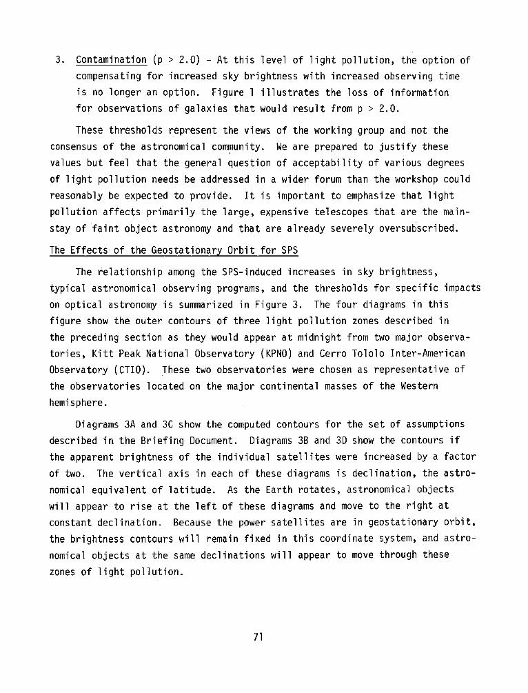
3. Contamination (p > 2.0) - At this level of light pollution, the option of compensating for increased sky brightness with increased observing time is no longer an option. Figure 1 illustrates the loss of information for observations of galaxies that would result from p > 2.0.

These thresholds represent the views of the working group and not the consensus of the astronomical com~unity. We are prepared to justify these values but feel that the general question of acceptability of various degrees of light pollution needs be addressed in a wider forum than the workshop could reasonably be expected to provide. It is important to emphasize that light pollution affects primarily the large, expensive telescopes that are the main­stay of faint object astronomy and that are already severely oversubscribed.

The Effects of the Geostationary Orbit for SPS

The relationship among the SPS-induced increases in sky brightness, typical astronomical observing programs, and the thresholds for specific impacts on optical astronomy is summarized in Figure 3. The four diagrams in this figure show the outer contours of three light pollution zones described in the preceding section as they would appear at midnight from two major observa­tories, Kitt Peak National Observatory (KPNO) and Cerro Tololo Inter-American Observatory (CTIO). These two observatories were chosen as representative of the observatories located on the major continental masses of the Western hemisphere.

Diagrams 3A and 3C show the computed contours for the set of assumptions described in the Briefing Document. Diagrams 3B and 3D show the contours if the apparent brightness of the individual satellites were increased by a factor of two. The vertical axis in each of these diagrams is declination, the astro­nomical equivalent of latitude. As the Earth rotates, astronomical objects will appear to rise at the left of these diagrams and move to the right at constant declination. Because the power satellites are in geostationary orbit, the brightness contours will remain fixed in this coordinate system, and astro­nomical objects at the same declinations will appear to move through these

zones of light pollution.

71

FIGURE 3. (A, B, C, D) Distribution of Predicted Increases in Diffuse Night Sky Brightness as a Result of a 60-Satellite System. A and B show the distribution of brightness as sun at midnight, the night of the vernal equinox, from KPNO. C and D show the distribution of brightness for the assumptions used in the Workshop Briefing Docu­ment that led to an apparent visual magnitude of -4.3 (as bright as Venus) for the individual satellites. The brightness distri­butions in B and D are the result of increasing the brightness of the satellites by a factor of 2. The map is an equal area pro­jection and the area enclosed with the horizon line is all of the sky that is visible at a given time from the respective observa­tories. The separate regions correspond to the impact threshold zones described in the text: 1) contaminated zone; 2) severe hindrance; 3) noticeable effect. Contours showing the fraction of the sky more than 30° above the horizon {z-60°) and 60° above the horizon (z=30°) are also shown for reference.

72

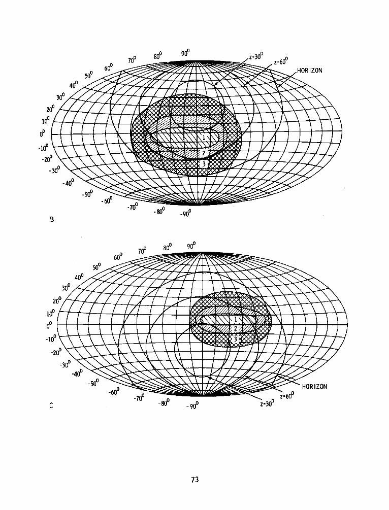
73

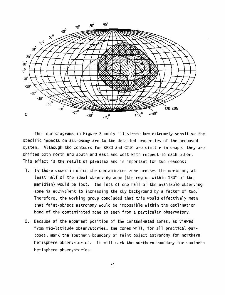
100

00

-10°

-20° ~~~mzJt;t;W -30°~ -40°

D -90°

The four diagrams in Figure 3 amply illustrate how extremely sensitive the specific impacts on astronomy are to the detailed properties of the proposed system. Although the contours for KPNO and CTIO are similar in shape, they are shifted both north and south and east and west with respect to each other. This effect is the result of parallax and is important for two reasons:

1. In those cases in which the contaminated zone crosses the meridian, at least half of the ideal observing zone (the region within %30° of the meridian) would be lost. The loss of one half of the available observing zone is equivalent to increasing the sky background by a factor of two. Therefore, the working group concluded that this would effectively mean that faint-object astronomy would be impossible within the declination band of the contaminated zone as seen from a particular observatory.

2. Because of the apparent position of the contaminated zones, as viewed from mid-latitude observatories, the zones will, for all practical ·pur­poses, mark the southern boundary of faint object astronomy for northern

hemisphere observatories. It will mark the northern boundary for southern

hemisphere observatories.

74

The north-south shift could be used to avoid a good fraction of the problems created by the contaminated zones if objects north of 0° declination

were always observed from KPNO while objects south of 0° were observed from

CTIO. However, in order to avoid the contaminated zones completely, these zones for the respective observatories must not overlap in declination. In Figures 3A and 3C the zones for CTIO and KPNO do overlap a small amount, creating a band between declinations -2° and +2° in which faint object astronomy would not be feasible from either observatory. This 4° band represents the minimum effect, reflecting the assumptions made in the Briefing Document. However, by

doubling the apparent brightness of the individual satellites (Figures0

3B and

30), this band is increased in width to 12°, more than one-tenth of the visible sky. This doubling would increase the width of the zone in which SPS is a severe hindrance to more than 40°, or approximately one-third of the sky. This condition dramatically illustrates a major concern of the working group-­that seemingly small deviations from the Briefing Document description of the SPS will result in a considerably amplified effect on optical astronomy.

A final consequence of the positioning of the satellites in geostationary orbits is illustrated in Figure 1 of the Briefing Document. This figure shows

the apparent position of the satellites as they would appear from several

observatories. The working group noted that if the satellites were positioned as described in the Briefing Document, Mauna Kea Observatory (MKO) in Hawaii would be far less affected by the SPS. The possibility that the Pacific Ocean area could be kept free of power satellites was perceived as an important possibility. This, however, would make Hawaii ineligible for power from the SPS.

EFFECTS ON OPTICAL ASTRONOMY

The primary effect of the SPS on optical astronomy is to contaminate a large region of the sky to the extent that the study of astronomical objects currently at the limit of detection would be impossible within that zone. The size of the region is extremely sensitive to the properties of the SPS and the

meteorological conditions at specific observatories. The impact is greatest for those observatories at longitudes nearest the center of the satellite

75

array. For the Reference System, the instruments most affected are those on the North and South American continents. The kinds of observations most affected are those currently limited by sky background.

The practical consequences for the research programs outlined in 11 Astronomical Observations: Scientific Programs 11 are as follows:

1. For those programs involving the study of randomly distributed objects, such as intrinsically faint stars and, in some respects, faint galaxies, the number of objects that can be studied will be reduced by an amount proportional to the fraction of the sky covered by the contaminated zones estimated between 3 and 10%. Further, these observations will be severely hindered in a region that may cover as much as a third of the sky.

2. Surveys designed to ascertain the cosmic distribution of objects may become subject to systematic errors stemming from the inability to study the whole sky.

3. Specific regions of the sky may be excluded from observation. Various parts of the sky provide a better opportunity to study particular classes of objects. The region most seriously affected by the Reference System is the ecliptic plane. Two regions are at the edge of the zones most noticeably affected, the galactic poles and the Virgo cluster of galaxies. These two areas of the sky are extremely important to extragalactic astronomy, and the working group expressed concern over the possibility that gross changes in the SPS configuration would render these areas unusable for many important kinds of observations.

4. Several important kinds of observations, type examples of classes of objects, will be lost to astronomy. These objects, as noted earlie~ are usually the nearest members of the class and are generally the subject of extensive observation and extremely detailed analysis, which is essen­tial to the identification of the physical processes that control the structure of the source. Examples of specific objects discussed that will fall within the contaminated zone include a) the Orion Nebula, a major testbed for theories of star formation; b) 3C273 and 3Cl20, two of the brightest quasistellar radio sources (Quasars); and c) NGC 1068, one of the brightest and closest galaxies that has an active nucleus.

76

5. Space astronomy may be faced with severe scheduling problems as outlined in Groth's paper.

A secondary effect of the SPS on optical astronomy is the potential impact on naked-eye astronomy. The human eye is a background-limited detector, and the increases in sky brightness as a result of the SPS will make such phenomena as the gegenschein, zodiacal light, and many comet tails invisible from North America. The visibility of the Milky Way will be reduced and the total number of stars visible will be reduced somewhat. These effects may have some impact on the identification of comets, novae, and other variable objects that are generally discovered by voluntary searches on the part of amateurs. The working group also expressed the concern that the SPS-induced changes in sky brightness may reduce the popularity of astronomy as a hobby and erode some of the excellent public support the field has enjoyed in the past. Several members of the group pointed out that the appearance of the night sky will be changed markedly, and that the aesthetics of the change were likely to be an issue and a concern.

Finally, the working group assessed the potential financial impact on a~tronomy. It was continually emphasized that an increase in sky brightness is equivalent to a reduction in telescope aperture. Currently, the price of a telescope scales as approximately the cube of the aperture. This means that to build a larger telescope to compensate for a 30% increase in sky brightness would increase the price of the telescope by approximately 120%.

RECOMMENDATIONS AND REMEDIES

Satellites as a source of light pollution are a phenomenon new to optical astronomy. While the working group attempted to assess as much of the poten­tial impact as possible, the information on which many of the conclusions were based was uncertain. For this reason, the working group recommended five areas requiring future study:

1. The diffuse albedo - Most of the effects discussed by the group are a direct function of the diffuse albedo. It was recommended that a) baffl­

ing systems be investigated as a way of lowering the albedo; b) each

77

design for the power satellite include a calculation of a meaningful estimate of the albedo and its potential for change over the orbital

lifetime of the system; and c) if active baffling is adopted, then the effect of its failure or any system failure on the albedo be estimated.

2. LEO structures - It was recommended that these structures be brought to a level of design at which their albedo can be computed and the impact assessed.

3. Atmospheric effects - It was recommended that a detailed calculation of

the effect of the satellites on sky brightness be carried out for those

meteorological conditions appropriate to real observatories.

4. Ionospheric heating - It was recorrmended that ionospheric and atmospheric

heating calculations be used to actually estimate the effects of emitted optical and IR radiation on astronomy.

5. Further assessment - It was recommended that a more permanent group be created within the optical astronomy community in order to monitor the potential impacts of the SPS and other orbital systems on optical astronomy.

Finally, the working group considered the possibility of mitigating the effect of the SPS on optical astronomy by performing the affected types of

study with telescopes in space. It was noted that the development of the technology required for the SPS should make it both easier and cheaper to construct and maintain space telescopes. It is also widely recognized that a great deal of the future of astronomy will depend on developing space astronomy

beyond current and planned levels and that some kinds of astronomy can only be

done from space.

Two problems were noted in association with any proposal that space astronomy might serve as a substitute for lost capability of ground-based

telescopes. First, ground-based facilities have historically been used to complement those studies made from space, and the effect of the SPS will be to

decrease that interaction. Second, it is always important to remember that

astronomy is an observational rather than an experimental science. It has not

78

always been obvious what the critical observations are or what the best instru­ments to pursue them will be. As a result, the diversity of astronomy has been a source of vitality in research. The working group felt that while astronomy from space is important and desirable, creating a single space facility to replace ground-based facilities would not preserve this vitality.

79

REPORT ON SPS EFFECTS ON AERONOMY

REPORT ON AERONOMICAL EFFECTS

The proposed SPS will have two effects on aeronorny. The first is analo­gous but not identical to the effect on optical astronomy, which is that the illumination of the night sky by the diffuse reflection from the SPS solar arrays will interfere with aeronomical observations. This effect is discussed both here and as part of the invited contribution of M. Davis which can be found in the radio effects section. Davis's remarks suggest that a substantial fraction of Arecibo's current optical aeronomy observations would be impossible following the construction of an SPS.

The second effect of the SPS creates an aeronomical phenomenon through the interaction of the microwave beam with the ionosphere. K. Clark's contri­bution, which follows, describes this effect.

In response to Clark's remarks, the optical astronomy working group con­cluded that the actual optical emissions that would result from the interaction should be predicted, which would allow their effect on optical astronomy to be assessed. The detailed analysis of ionospheric effects is another element of the current DOE/NASA SPS assessment, and, hopefully, that portion of the assess­ment will result in a prediction of the optical emissions.

83

EFFECTS ON AERONOMY OBSERVATIONS

K. Clark

INTRODUCTION

The feasibility of establishing a belt of up to three-score geosynchronous solar power satellites can be considered from an aspect that is neither mundane nor celestial but which concerns the earth's upper atmosphere. We can ask, what optical effects of the satellites would be important to the growth or inhibition of our scientific understanding of the distant atmosphere? Because the future is unknown, these effects are an open-ended topic, but quantitative assessments of some of the recognizable impacts of aeronomical effects have been published and will be used in the following comments.

The deposit of energy by the radio frequency beam coming through the iono­sphere occurs in a geographically local region. The region's vertical and lateral extent is limited by ionospheric electron concentration and by beam width, and so the range of its view from the ground is roughly only several hundred kilometers. Significant increases of light emission are anticipated in this deposition region. An additional, different concern is the direct viewing of a well illuminated satellite from the ground, seen permanently from nearly all the Western hemisphere. Both of these effects would influence our study of the upper atmospheric environment.

LOCAL HEATING

Concentrations of free electrons are greatest in the ionospheric F region· broadly from 200 to 350 km, remain significant in the E region from 100 to 150 km, and are appreciable down to the D region around 80 km. The intense electric field in the RF beam transfers a fraction of the beam power into heating the available electrons en route. The field raises their temperature and, by their subsequent collisions, the energy of the atmospheric con­stituents. The temperatures, or average energies, of electrons, ions, and

85

neutrals are set by the balancing of all processes for energy gain and loss, and the RF beam is a noteworthy contributor.

The electron heating rate Q per unit volume in the beam is proportional to several factors:

where

Q ~ E2 (n /f2) (f. + f) e , n

E = beam electric field f = beam frequency

n = e f. =

l

electron concentration electron-ion collision frequency

f n = electron-neutral collision frequency

To determine the dominant loss processes for electron heat energy, one must consider details of the atmospheric composition, the relevant collision cross sections, and the interplay of mean free path, thermal conduction, and magnetic confinement. Recently, Perkins and Roble (1978) (hereinafter PR) have numerically evaluated the resultant effects of these processes in standard mid­latitude atmospheres with typical RF heating. They point out the comparability of effects from the low-frequency Arecibo antenna (15 MHz, 1 to 3 MW) and from a possible satellite power station (2.45 GHz, 10 GW).

In the low D and E regions, the heated free electrons lose energy mostly by collisions exciting rotational and vibrational states of the major moelcules N2 and o2• Since these homonuclear molecules cannot radiate the energy, it is collisionally transferred to and emitted by co2 (4.3 µ) and H2o (6.5 µ),

respectively. Throughout the E region the abundant atomic 0 provides for elec­tron energy loss by the excitation of fine structure levels in ground state 0( 3P}. Also, Coulomb collisions of electrons and ions are significant. In the more highly ionized F region, principal electron energy degradation is by elec­tron Coulomb collisions and by electron-spin exchange collisions producing metast­able o( 1o) and its subsequent 6300A emission. A list of the above follows:

86

D, E regions: e + N2 _. e + N2*(r,v)

N/ + co2 -+ N2 + C02* (-+ 4. 3 µ)

e + o2 _. e + o2*(r,v) 02* + H20 _.. o2 + H

20 *( -+ 6. 5 µ )

E region: e + 0( 3P) - e + o*( 3P) + e, M : Coulomb collisions

F region: e + 0{ 3P) - e + o*( 1o) e, e: Coulomb collisions

The loss of electron energy by thermal conduction out of the beam is slow below 150 km because of the small mean free path. The incident RF beam intersection determines the form of the hot region. Above about 200 km, heat conduction is magnetically confined transverse to the magnetic field direction but is good parallel to the field. Some illustrations from PR are reproduced here, by permission.

Figure 1 shows energy loss rates versus height for certain of the atmo­spheric products, using a daytime model atmosphere with and without irradiation by the assumed RF beam. Large effects near 100 km are to be noted. The assumed satellite beam of 10 GW is taken parallel to the field. Figure 2 shows the daytime intensity distribution of 0(1D) 6300A emission near Boulder as affected by the satellite beam. The maximum heating curve takes the beam parallel to the field; the others are for indicated intersections of the beam with the field line at heights of 200, 250, and 350 km. Even with the strong daytime photoproduction, one sees pronounced enhancements caused by the added beam.

GREAT LOCAL HEATING

So-called runaway thermal heating is an interesting possibility in ionospheric radio-frequency heating, as discussed by Holway and Meltz (1973) and others. The inception of thermal runaway can be noted in ground-based studies with very large antennas. The higher the electron temperature becomes, the greater is the ability to transfer RF energy via collision frequency. The loss rates for electron energy are lessened as electron

87

temperature rises and as heat conduction becomes restricted at low heights, and it is thereby quite possible to produce a localized great enhancement of temperature. Figure 3 from the PR calculations for Arecibo illustrates that the temperature at low altitudes rises faster with beam power than it does at higher altitudes. With sufficient and attainable power, the assumed loss processes are unable to control the increasing heat gain. Unbounded runaway temperatures, however, refer only to the modelled processes; actual limiting would occur at sufficiently high temperatures as ignored loss channels become more important.

The production of thermal runaway temperatures in the low (50 to 100 km) portion of a strong RF beam is an intriguing, though not catastrophic, result of intense atmospheric RF heating. It is seen in the example of Figure 4, which gives the calculated meridional distribution of Te at Boulder for various intersection heights of the beam with the field line. Temperature rises of 700°K are indicated at the high F region electron concentrations, though good conduction is a mediator. The runaway effect, however, is shown below 100 km by the unlimited breakthrough of temperature contours. The nonlinear effects that develop in such a regime make accurate calculations unsure. It should be emphasized that no tendency toward runaway becomes noticeable until the beam power is very intense.

LOCAL OPTICAL RESULTS

The natural excitation of upper atmospheric emissions comes from:

• Direct excitation by daytime photons (effectively a few to 20 eV) • Direct photoionization and excitation (10 to 20 eV) • Collisions with secondary photoelectrons (effectively a few to 20 eV) • Dissociative recombination of molecular ions and electrons (several eV) • Chemical reactions yielding excited products (a few eV) • Collisions with energetic electrons (auroral 0.5 to 10 keV, and

secondaries) • Collisions with superthermal electrons from plasmasphere (to 100 eV) • Minor contribution from energetic incident ions (0.5 to 30 keV)

88

The beam-heated electrons provide at most a few eV of energy, and their effect is considered to be only on the very low-lying energy states. The two lowest-lying metastable states of o2, a1Eg and b16g, yield infrared bands at 1.27 µ and 0.86 µ, respectively, and would show abnormal intensity in

0

the region below 100 km. The forbidden 0 6300,6364A doublet would, as noted, show abnormal brightness in the F region, where deactivation collisions are infrequent. The 4.3-µ and 6.5-µ emission enhancement for co2 and H2o at low altitudes has been mentioned previously. Only at highly pronounced runaway heating below 100 km would higher energy states of available constituents be appreciably excited by the beam; the next highest metastable atomic oxygen state, for example, requires about 4 eV and yields the bright

0

green auroral and airglow line at 5577A. While normally the electron and neutral temperatures at low (below 100 km) altitudes are essentially equal, RF heating would raise the Te several times greater than Tn and thereby lead to the various excitations. Another complex result would come from the fact that a small fraction of the electron heat is not radiated away but is transferred to heating the neutral components; the enhanced reaction rates of the processes of atmospheric chemistry for the many constituents of the D region will not be analyzed here.

The effect at heights below 100 km, seen locally for the infrared emissions by co2, H2o, and o2, might roughly double the naturally

0

occurring intensities. The normal daytime intensity of 6300A, peaking around 250 km and coming to a total of about 4 kilorayleighs, comes mostly from photoelectrons, photodissociation, and dissociative recombination with only about 1% from thermal electron impact. The RF heating would bring the latter contribution up to several kilorayleighs itself. At night especially, this heating would be the dominant source of the light, and the glow could be faintly visible as well as highly measurable. It would be as bright as a good stable auroral red arc (SAR arc) at midlatitudes, and equivalent to a weak auroral display.

While it is conceivable that special studies of processes might take advantage of the uniquely localized parameters within the beam, the masking effect of the artificial excitation would vitiate most studies of the natural

89

upper atmospheric environment using these standard emissions within a ground radius of 300 to 1000 km, depending on height and project.

WIDESPREAD EFFECTS

A more pervasive consideration is the permanent and general illumination by a belt of sunlit satellites, whose finite reflectivity produced light estimated as brighter than perhaps 0.1 of a full moon. This light is seen not only close to the sources via small angle scattering but also is distributed more or less over the sky seen from a ground station, depending on the prevalence of fine haze. We note, but set aside here, the interactions of this background light with astronomy. In optical studies of the upper atmosphere itself, much research rests on ground-based spectrophotometric measurements of the faint light emissions, which give information on the energy delivered within the sun's outer environment of particles, waves, and radiation. How the solar wind energizes the earth's magnetosphere is traced by the pattern of auroras formed by incident electrons, and the chemistry of upper atmospheric processes is shown by the airglow.

This highly developed science depends on measurement of faint-sky light, accurately discriminated as to wavelength, intensity, and variations with time and space. The airglow, with all its spectral components, is roughly equal to astronomical sources in providing the brightness of the dark sky. Intensities of auroras, which cover a wide range in various circumstances, often approach those of the airglow while yet maintaining much information content. Especially at midlatitudes, the subvisual stable auroral red arcs and the diffuse auroras require very sensitive spectral measurement and are unique indicators of the plasmapause region of the magnetosphere. Much future study will center on relatively weak emissions extending from the near ultraviolet to the near infrared. Many measurements press detection sensitivity to the limits of background light. The SAR arcs are reliably mapped and measured over the sky at levels of 50 Rayleighs. High-resolution studies of Doppler shifts in thermospheric winds are at the limit of photon statistics. The

airglow continuum is already compromised by natural backgrounds, and the artificial light would directly overwhelm it in any but the best conditions.

90

Weak band emissions from minor atmospheric components would find obvious competition from scattering. The numerical estimates of limits cannot well be reckoned because of the variable stringencies of different experimental tasks, the ranges of thin haze cover, and the various contributions from aerosol and Rayleigh scattering. Effects would translate into reduced hours and poor intensity discrimination.

Actual examples are probably the best evidence. Moonlight now limits the validity of ground-based spectrophotometric measurements. Typically, a quarter moon sets the limit on photometry anywhere in the clear sky, and for many studies the moon cannot be present in any phase of its brightness. The emission by incident hydrogen, regardless of its Doppler profile, is an important observational link in magnetospheric interaction studies; the blue H-beta line is the best to use, and narrow interference filters are variously employed for it. The villainy of scattered moonlight is heightened by the structure of Fraunhofer absorption lines in the solar spectrum near H8; spurious results can come from scanning the filter pass band because of the contaminating scattered light from the sky. The moon must be gone.

The moon would never be gone, at any hour or any day, if the satellites contributed the equivalent of a 1/8 crescent. The background solar spectrum scattered in the dark hours would effectively end many desired aeronomic studies based on faint airglow and aurora.

REFERENCES

Perkins, F. W. and R. G. Roble, Journal of Geophysical Research. 83(A4): 1611-1624, 1978.

Holway, L. H., Jr. and G. Meltz, Journal of Geophysical Research. 78(A34): 8402-8408, 1973.

91

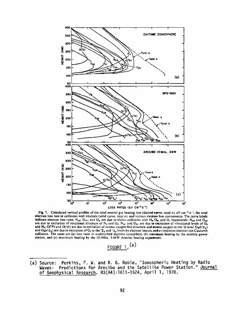
DAYTIME IONOSPHERE

(a)

SPS-MAX

ARECl80 IS MHz, 3MW

(c)

101 10• 104

LOSS RATES (EV CM-3 5-1)

Fig. 7. Calculated vertical profiles of the total neutral gas heating rate (dashed curve, total 11), eV cm-• s- •. the total electron loss rate in collisions with neutrals (solid curve, total e), and various electron loss components. The curve labels indicate electron loss rates; N,1:. 0,,., and 01: arc due to elastic collisions with N., Os. and 0, respectively: N2H and 0211 are due to excitation of rotational structure of N2 and O,; N2V and O.v are due to excitation of vibrational levels of O, and N1: O('P) and O('D) are due to excitation of atomic oxygen fine structure and Momic oxygen to the 'D level. 0.(b'l:,) and 0 2(a'A.l are due to excitation of02 10 the 1.2:, and '<l, levels by electron impact,andt'-i indicates electron-ion Coulomb collisions. The cases arc (a) loss rates in undisturbed daytime ionosphere, (b) ma.,imum heating by the satellite power station, and (c) m:1ximum heating by the 15-MHz. 3-MW Arecibo heating experirne111.

(a)

FIGURE 1. (a)

Source: Perkins, F. W. and R. G. Roble, 11 Ionospheric Heating by Radio Waves: Predictions for Arecibo and the Satellite Power Station. 11 Journal of Geophysical Research. 83(A4):1611-1624, April l, 1978.

92

200

100 8~~00,,___._~_._....._L.L.L~~,~-'-.............. ~ ...... ~~.~ ........................ o...wu...u~~,

6300-A VOLUME EMISSION RATE (photons cm"3 !11)

Fig. 8. The calculated vertical profile of the 6300-A volume emis­sion rate: (photons cm·• s· 1

). The solid curve is the volume emission rate in the undisturbed daytime ionqsphere, and the long dashed-short dashed curve is the emission rate calculated for maximum heating by the satellite power station. the dashed curves are volume emission rates calculated over Boulder along geomagnetic field lines that inter­sect the radio wave beam at 200, 250, and 350 km, respectively.

FIGURE 2. (a)

~ ~ ~ 5 0 5 ~ ~ ~

DISTANCE (km)

OO I 2 3 4 5 HEATING POWER (MW)

Fig. 16. Relationship between electron temperature and heating power for an Arecibo heating experiment at various altitudes in the D and E regions.

FIGURE 3. (a)

Fig . .4. Contours of calculated electron temperature (in degrees Kelvin) over Boulder for radio wave heating by the satellite power station. The dashed lines give the radio wave beam direction, and the light solid lines indicate the geomagnetic field direction.

FIGURE 4. (a)

(a) Source: Perkins, R. W. and R. G. Roble, "Ionospheric Heating by Radio Waves: Predictions for Arecibo and the Satellite Power Station." Journal of Geophysical Research. 83(A4):1611-1624, April 1, 1978.

93

INVITED PRESENTATIONS ON SPS EFFECTS ON RADIO ASTRONOMY

MICROWAVE POWER TRANSMISSION SYSTEM

G. D. Arndt

The SPS microwave system has DC-RF power converters feeding a 1-km­diamet~r phased array antenna with a 10-decibel (dB) Gaussian illumination taper across the array surface. This system, as described on pages 25-46 of the SPS Reference System Report, DOE/ER-0023, dated October 1978, has not been significantly altered to date (May 1979). There are, however, two microwave areas with new analyses available now: l) scattered power as a function of electrical and mechanical tolerances, and 2) grating lobe characteristics when the phase control system conjugates at the power module (tube) level rather than at the subarray level.

SCATTERED POWER AT 2450 MHz

Microwave interference with communications and navigation systems and radio astronomy will come primarily from three spacetenna sources: sideband radiation from the 2450-MHz main power beam, harmonics of 2450 MHz generated by the DC-RF converter tubes, and tube noise outside the IMS frequency band (2450 ± 50 MHz). In addition, there will be reradiation and reflections from the rectenna. A considerable amount of power at 2450 MHz will be scattered into the side lobes due to electrical and mechanical tolerances within the antenna. Figure l gives the microwave power lost due to these tolerances; i.e., 2% tube failures, 10° phase error, 3 arcmin subarray tilt, ±1 dB ampli­tude error across the subarray or power module surface, l arcmin antenna tilt, and a 0.25-inch mechanical spacing between the subarrays. Tube failures produce the largest loss in rectenna power (268 MW) because of the reduction in antenna area and in the amount of transmitted power. Random phase errors and 3 arcmin random subarray tilt each produce 188 MW of scattered power. The other error sources combine to scatter about 100 MW of power.

There are two types of errors within the SPS phase control system which indirectly affect astronomers:

97

300

:!: ~ er:::

200 LL.I

:!: 0 Cl. LL.I > <(

:!: 0 O:'. u :iE 0 1()() LL.I O:'.

~ <( u Vl

0

268

2% FAILURES

100 PHASE ERROR

-3-MIN 1-dB RANDOM AMPLI TUOE

SUBARRAY ERROR TILT

1-=Mi"N ANTENNA

TILT

.25-IN. SPACING BETWEEN

SUBARRAYS

FIGURE 1. Scattered Microwave Power Due to Electrical and Mechanical Errors

l. Random - due to errors in the RF receiver/conjugation electronics, power tubes, ionospheric perturbations on the uplink pilot beam signal, sub­array misalignment, and errors in the upper levels of the phase reference distribution system within the antenna. These errors scatter the main beam power and result in higher side lobe levels.

2. Correlated - due to errors in the first and second levels of the refer­ence distribution system within the antenna. These errors produce a main beam pointing error of approximately 25 meters/ degree of correlated error.

In summarizing the phase error effects, 10° of error produce 188 MW of scattered power and a maximum beam misalignment of 250 m from rectenna foresight.

98

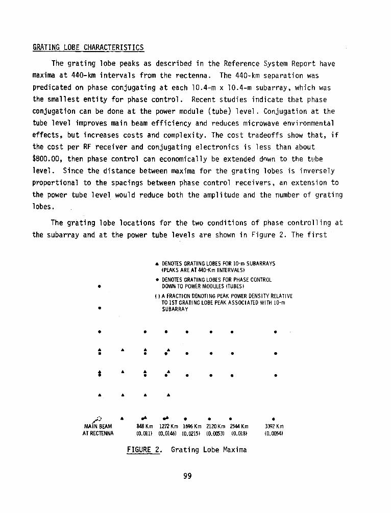
GRATING LOBE CHARACTERISTICS

The grating lobe peaks as described in the Reference System Report have maxima at 440-km intervals from the rectenna. The 440-km separation was predicated on phase conjugating at each 10.4-m x 10.4-m subarray, which was the smallest entity for phase control. Recent studies indicate that phase conjugation can be done at the power module (tube) level. Conjugation at the tube level improves main beam efficiency and reduces microwave environmental effects, but increases costs and complexity. The cost tradeoffs show that, if the cost per RF receiver and conjugating electronics is less than about $800.00, then phase control can economically be extended dnwn to the tube level. Since the distance between maxima for the grating lobes is inversely proportional to the spacings between phase control receivers, an extension to the power tube level would reduce both the amplitude and the number of grating lobes.

The grating lobe locations for the two conditions of phase controlling at the subarray and at the power tube levels are shown in Figure 2. The first

• DENOlIS GRATING LOBES FOR 10-m SUBARRAYS !PEAKS ARE AT 440-Km INTERVALS I

• DENOlIS GRATING LOBES FOR PHASE CONTROL

• DOWN TO POWER MODULES ITUBESl

I l A FRACTION DENOTING PEAK POWER DENSITY RELATIVE TO lST GRATING LOBE PEAK ASSOCIAlID WITH 10-m

• SUBARRAY

• • • • • • •

• • • • • • • • • •

t • • • • • • • •

• •

. -, /' • .. .. • • • •

MAIN BEAM 848 Km 1272 Km 1696 Km 2120 Km 2544 Km 3392 Km AT REClINNA IO.Olll I0.0146) I0.02151 I0.0053) I0.0181 !0.0054)

FIGURE 2. Grating Lobe Maxima

99

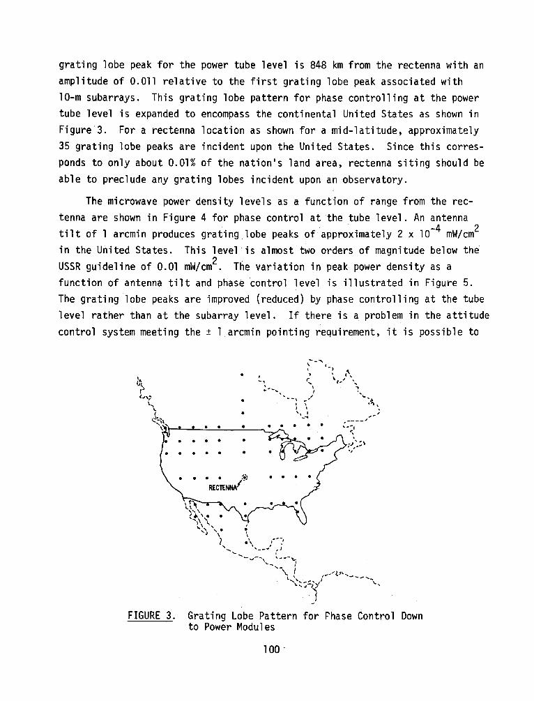
grating lobe peak for the power tube level is 848 km from the rectenna with an amplitude of 0.011 relative to the first grating lobe peak associated with 10-m subarrays. This grating lobe pattern for phase controlling at the power tube level is expanded to encompass the continental United States as shown in Figure 3. For a rectenna location as shown for a mid-latitude, approximately 35 grating lobe peaks are incident upon the United States. Since this corres­ponds to only about 0.01% of the nation's land area, rectenna siting should be able to preclude any grating lobes incident upon an observatory.

The microwave power density levels as a function of range from the rec­tenna are shown in Figure 4 for phase control at the tube level. An antenna tilt of l arcmin produces grating lobe peaks of approximately 2 x 10-4 mW/cm2

in the United States. This level is almost two orders of magnitude below the USSR guideline of 0.01 mW/cm2. The variation in peak power density as a function of antenna tilt and phase control level is illustrated in Figure 5. The grating lobe peaks are improved (reduced) by phase controlling at the tube level rather than at the subarray level. If there is a problem in the attitude control system meeting the ± l arcmin pointing requirement, it is possible to

• • • • • • • • • • • •

. . . . :•: RECTENN-1-

FIGURE 3. Grating Lobe Pattern for Phase Control Down to Power Modules

100.

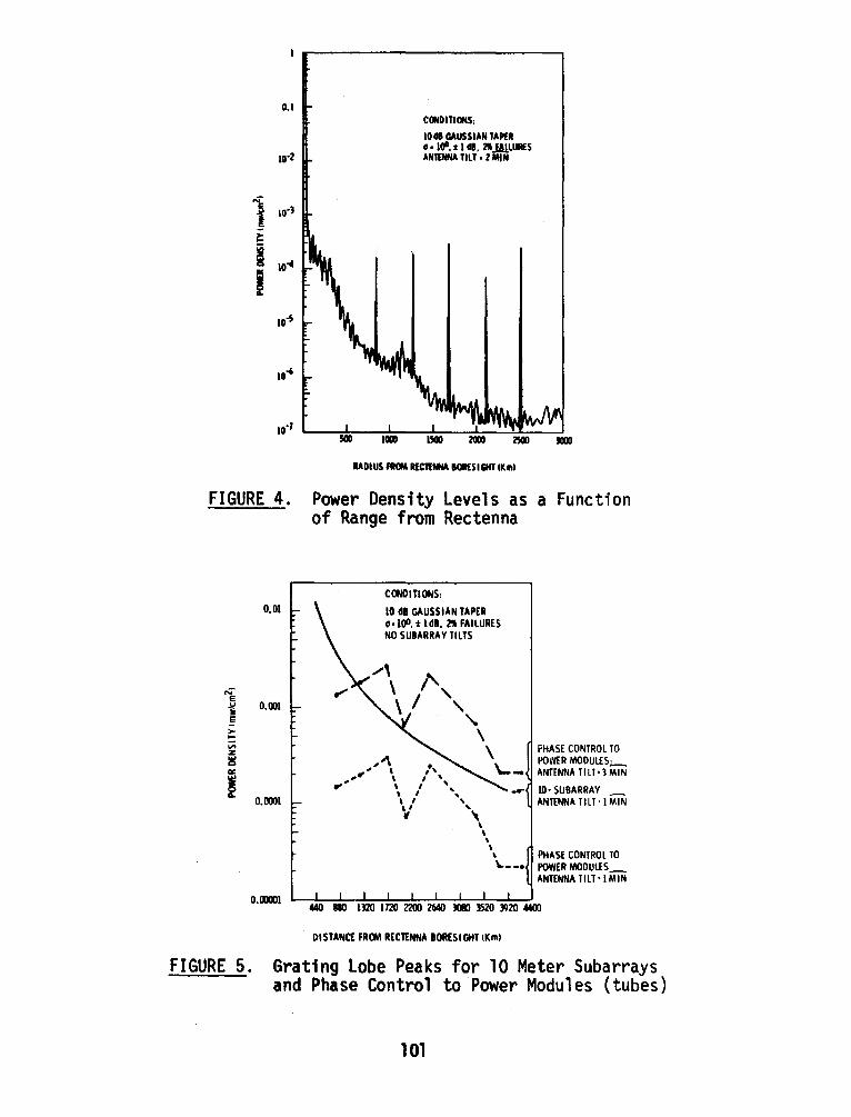
0.1 CONOITHlNS:

10 di GAUSSIAN TAP£R o -100. :t I di, 21 ..fAllUll£S AN'ltNNA TILT• 2 MIN

RADIUS FROM lllC'llNNA IOR£51GHT CKml

FIGURE 4. Power Density Levels as a Function of Range from Rectenna

i ~ • E

> ... "' z ~

"' ~

0.01

0.001

O.<ml

O.lmll

CONDITIONS:

10 dB GAUSSIAN TAPER 0• 100. :I: ldB, 2'Tt FAILURES NO SUBARRAY TILTS

I', I '

,,A, •, .,,.. \ I '

.,- ' / '" ' I '

'\, \ \

\ / ', w ' \

' ' \ \

PHASE CONTROL TO POWER MODULES;._ ANTENNA TILT• 3 MIN

_... IO· SUBARRAY _ ANTENNA TILT· I MIN

\. ... PHASE CONTROL TO POWER MODULES_ ANTENNA TILT· I MIN

.t40 1110 1320 1720 Z200 2640 D10 3520 3920 4400

DISTANCE FROM RECTENNA BORESIGHT OCml

FIGURE 5. Grating Lobe Peaks for 10 Meter Subarrays and Phase Control to Power Modules (tubes)

101

raise the pointing standard to ±3 arcmin and still be in the 0.001 mW/cm2

power density range. The analysis also indicates the grating lobe peaks are very sensitive to changes in antenna or systematic tilt but are relatively insensitive to random or subarray tilts. Hence, the ±3 arcmin subarray tilt requirement is independent of the phase control level.

In sunrnarizing the advantages of phase controlling at the power tube level, the grating lobe peaks are wider spaced and the magnitudes are 1/10 to 1/100 of those for 10-m subarrays. Proper rectenna sitings should exclude radio astronomy observatories from grating lobe locations.

1~

SPS NOISE AND HARMONICS

R. M. Dickinson

NOTE: Although Dr. Dickinson was unable to attend the workshop, he has con­tributed copies of the slides prepared in support of his invited presentation.

SLIDE 1

BEAMED RF POWER TECHNOLOGY MICROWAVE SUBSYSTEM CHARACTERISTICS FOR SPS SYSTEM DESIGNERS AND ANALYST

• RECTENNA SCATTERING, SPILLOVER & HARMONICS PATTERNS

11-IE INTRODUCTORY VIEWGRAPH COLLAGE DEPICTS THE MAJOR PORTIONS OF TI-IE JPL BEAMED RF POWER TECHNOLOGY TASK FOR NASA.

RF PERFORMANCE CHARACTERISTICS SUCH AS NOISE LEVELS, HARMONIC PAffiRNS AND ARRAY POINTING ACCURACY ARE BEING MEASURED FOR DC TO RF CONVERTERS, TRANTENNAS AND RECTENNAS.

11-IE MEASURED DATA ARE USEFUL FOR SPS SYSTEM DESIGNERS AND ANALYSTS TO ASSIST IN DETERMINING THE MAGNITUDE OF AND TO MINIMIZE THE POTENTIAL RF INTERFERENCE TO OTHER SPECTRUM USERS.

104

SLIDE 2

BEAMED RF POWER TECHNOLOGY

CURRENT ACTIVITIES

1. DESIGNING, FABRICATING & ASSEMBLING AN 8-ELEMENT ACTIVE RETRODIRECTIVE ARRAY (ARAI MODEL & INSTRUMENTATION FOR VERIFICATION TESTING OF BEAM FORMING AND POINTING ACCURACY

2. MEASURING PERFORMANCE CHARACTERISTICS OF de TO RF CONVERTERS

3. RECORDING RADIATED HARMONICS OF RECTENNAS AND SLOffiD WAVEGUIDE ANTENNAS

PLANNED ACTIVITIES

1. CONDUCT EXTENSIVE ARA PERFORMANCE MEASUREMENTS

2. RECORD ARA HARMONIC PAffiRN DISTRIBUTIONS

3. INVESTIGATE TECHNIQUES FOR REDUCING ARRAY HARMONIC LEVELS

THE CURRENT AND PLANNED ACTIVITIES ARE LISTED FOR THE BEAMED RF POWER TECHNOLOGY TASK AT JPL.

SUBSEQUENT VIEWGRAPHS WILL PRESENT PRELIMINARY MEASUREMENT RESULTS IN SELECTED TECHNOLOGY AREAS. WHILE THE RES LILTS ARE NOT I DENTtcAL TO EXPECTED FU GHT HARDWARE OR GROUND EQUIPMENT, THEY ARE FELT TO BE REPRESENTATIVE OF THE VERY COMPLEX AND, IN SOME CASES, ALMOST INCALCULABLE RESULTS OF HARMONIC PERFORMANCE AND, AS SUCH, SHOULD BE OF VALUE TO DESIGNERS AND ANALYST.

A JPL TECHNICAL REPORT IS BEING PREPARED ON THE NOISE AND HARMONIC DATA. A SEPARATE, LATER REPORT WILL DEAL WITH THE ARRAY BEAM POINTING.

105

SLIDE 3

BEAMED RF POWER TECHNOLOGY TRANSMITTING PHASED ARRAY

RFI, NOISE AND HARMONICS TRANSMITIING ARRAY GENERATOR CHARACITRISTICS, TRANSMISSION

cor.\PONENTS AND RADIATION TRANSFER FUNCTIONS

1. de -RF ------1. PHASE JITTER, am, LINEWIDTH, NOISE, SPURIOUS, CONVERTER- -- --~ - -- ---- HARMONICS

2. WAVEGUIDE RF ..... 2. GU IDE MODES, IMPEDANCES, TERMINATIONS

COLLECTION-- --- - - - - - ----- ,_ __ ................... 3. SKIRT WIDTH, REJECTION, INSERTION LOSS, 3. NOISE BAND PASS

LIMITING AND HAR- , .. PASSBAND RIPPLE

MONICFILTERING--------- .......... - 4. CHANNEL SEPARATION, JNANDOUTOFCHANNEL 4. PILOT SIGNAL- ,,,,.ATTENUATIOtl:, BANDWIDTHS

PO\VER SIGNAL DI- ,,,,..,.,,,,. .. 5. GUIDE MODES, IMPEDANCES, TERMINATIONS, PLEXING FILTER - _

---- .,.,,,,.,,.. AMPLITUDE POWER SPLIT UNIFORMITY, PHASE AND -- ~..,,."' ,.AMPLITUDE STABILITY

SPATIAL, SPECTRAL AND TEMPORAL DI STR I BUT ION OF EMITTED ENERGY

A SIMPLIFIED SCHEMATIC ILLUSTRATING THE COMPONENTS AND THEIR ASSOCIATED PARAMETERS IN THE COMPLEX CHAIN FROM RF GENERATOR TO RF RADIATOR.

THE RADIATED ANTENNA PAITTRNS OF HARMONICS ARE ESPECIALLY COMPLEX BECAUSE OF THE MULTI-MODE NATURE OF HARMONIC PROPAGATION. THE IMPEDANCE AT THE HARMON! C FREQUENCIES THAT IS PRESENTED TO THE CONVERTERS ALMOST DEFIES CALCULATION. THUS, UNTIL TYPICAL HARDWARE IS AVAILABLE, ONLY "REPRESENTATIVE, 11 INSTEAD OF ACTUAL HARMONIC, PAITTRNS ARE AVAILABLE.

l 06

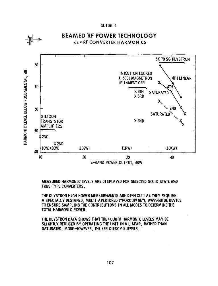
80 co -0

_j

~ z 70 LaJ

:E <C 0 :z ::::> LL.

3: 0

60 -' LaJ a:i

-' LaJ

~ u z 50 0 :E a:: <C :c

40

SLIDE 4

BEAMED RF POWER TECHNOLOGY dc--RF CONVERTER HARMONICS

.SK 70 SG KLYSTRON

SILICON TRANSISTOR AMPLIFIERS

2ND

X2ND (lOWl !20Wl

10

INJECTION LOCKED L-5001 MAGNETRON !FI LAMENT OFF)

X 4TH X 3RD

~

X2ND

'- 2ND

SATURATED'-'

(lOGW) UKWl (lOKWl

w ~ 40 S-BAND POWER OUTPUT, dBW

MEASURED HARMONIC LEVELS ARE DISPLAYED FOR SELECTED SOLID STATE AND TUBE-TYPE CONVERTERS.

THE KLYSTRON HIGH POWER MEASUREMENTS ARE DIFFICULT AS THEY REQUIRE

\

A SPECIALLY DESIGNED, MULTI-APERTURED ("PORCUPINE"), WAVEGUIDE DEVICE TO ENSURE SAMPLING THE CONTRIBUTIONS IN ALL MODES TO DETERMINE THE TOTAL HARMONIC POWER.

THE KLYSTRON DATA SHOWS TH!fT THE FOURTH HARMONIC LEVELS MAY BE SLIGHTLY REDUCED BY OPERATING THE UNIT IN A LINEAR, RATHER THAN SATURATED, MODE+IOWEVER, THE EFFICIENCY SUFFERS.

107

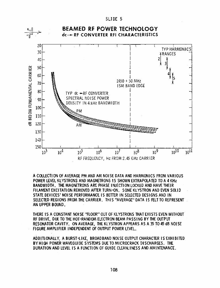
SLIDE 5

!'";"\!1 -b·itu-=-

BEAM.ED RF POWER TECHNOLOGY de- RF CONVERTER RFI CHARACTERISTICS

c:: LI.I

c:: e::: <X: u __J

< I-z LLJ :?:: <X: 0 z => """" 3: 0 ...... LI.I a:::i

c::c "C

20

30

40

50

60

70

80

. 90

100

llO

120

130

140

150 103

TYP de -RF CONVERTER SPECTRAL NO I SE POWER

I I I I I I

2450 + 50 MHz I SM BAND EDGE

I I

oms ITY IN 4 kHz BANDWIDTH I I I I I

ia5 RF FREQUENCY, Hz FROM 2.45 GHz CARRIER

A COLLECTION OF AVERAGE PM AND AM NOISE DATA AND HARMONICS FROM VARIOUS POWER LEVEL KLYSTRONS AND MAGNETRONS IS SHOWN EXTRAPOLAlED TO A 4 KHz BANDWIDTH. THE MAGNETRONS ARE PHASE INJECTION LOCKED AND HAVE THEIR FILAMENT EXCITATION REMOVED AFlER TURN-ON. SOME KLYSTRON AND EVEN SOLID STAlE DEVICES' NOISE PERFORMANCE IS BETTER IN SELECTED DESIGNS AND IN SELEClED REGIONS FROM THE CARRIER. THIS "AVERAGE" DATA IS FELT TO REPRESENT AN UPPER BOUND.

THERE IS A CONSTANT NOi SE "FLOOR" OUT OF KLYSTRONS THAT EXISTS EVEN WITHOUT RF DRIVE, DUE TO THE HOT-RANDOM ELECTRON BEAM PASSING BY THE OUTPUT RESONATOR CAVITY. ON AVERAGE, THE KLYSTRON APPEARS AS A 35 TO 45 dB NOi SE FIGURE AMPLIFIER INDEPENDENT OF OUTPUT POWER LEVEL. .

ADDITIONALLY, A BURST-LIKE, BROADBAND NOi SE OUTPUT CHARAClER IS EXHI BllED BY HIGH POWER WAVEGUIDE SYSlEMS DUE TO MICROCRACK DISCHARGES. THE DURATION AND LEVEL IS A FUNCTION OF GUIDE CLEANLINESS AND MAINlENANCE.

108

I ---,

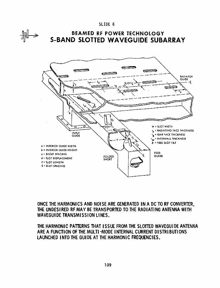
SLIDE 6

BEAMED RF POWER TECHNOLOGY

S-BAND SLOTTED WAVEGUIDE SUBARRAY

INPUT GUIDE

a= INTERIOR GUIDE WIDTH

b • INTERIOR GUIDE HEIGHT

c = SHORT SPACING

d = SLOT DISPLACEMENT

l = SLOT LENGTH S = SLOT SPACING

FOLDED SHORT

re: s E 3

-------

--------------

W = SLOT WIDTH

tF = RADIATING FACE THICKNESS

18 = REAR FACE THICKNESS

tW ~ INTERWALL THICKNESS

0 =FEED SLOT TILT

FEED GUIDE

ONCE THE HARMON I CS AND NOi SE ARE GENERATED IN A DC TO RF CONVERTER, THE UNDESIRED RF MAY BE TRANSPORTED TO THE RADIATING ANTENNA WITH WAVEGUIDE TRANSMISSION LINES.

THE HARMONIC PATTERNS THAT ISSUE FROM THE SLOTTED WAVEGUIDE ANTENNA ARE A FUNCTION OF THE MULTI -MODE INTERNAL CURRENT DI STR I BUTI ONS LAUNCHED INTO THE GUIDE AT THE HARMONIC FREQUENCIES.

109

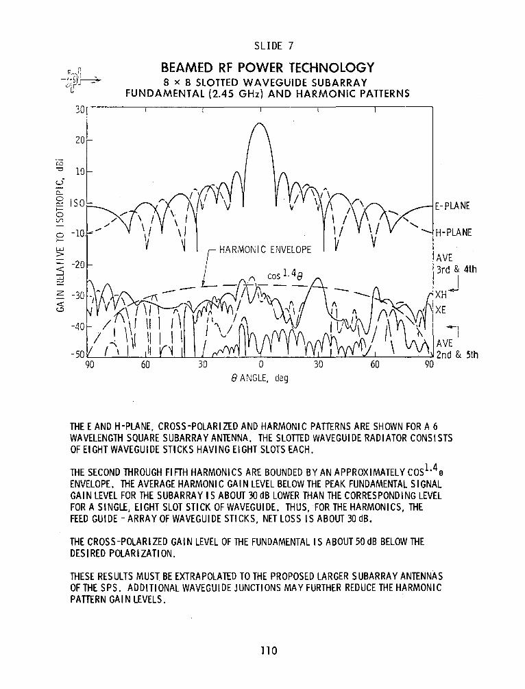
30

20

cc

SLIDE 7

BEAMED RF POWER TECHNOLOGY 8 x 8 SLOTTED WAVEGUIDE SUBARRAY

FUNDAMENTAL (2.45 GHz) AND HARMONIC PATTERNS

u 10 c3

S I S0'- E-PLANE 1-0 V1

0 r--w > ,.... ::i ~ z -<( ~

-10. H-PLANE

-20 AVE 3rd & 4th

-30 -- XHj

-40

-50 90 60 30 0 30

8 ANGLE, deg

THEE AND H-PLANE, CROSS-POLARIZED AND HARMONIC PAffiRNS ARE SHOWN FOR A 6 WAVELENGTH SQUARE SUBARRAY ANTENNA. THE SLOffiD WAVEGUIDE RADIATOR CONS! STS OF EIGHT WAVEGUIDE STICKS HAVING EIGHT SLOTS EACH.

THE SECOND THROUGH FIFTH HARMONICS ARE BOUNDED BYAN APPROXIMATELYCOSl.4e ENVELOPE. THE AVERAGE HARMONIC GAIN LEVEL BELOW THE PEAK FUNDAMENTAL SIGNAL GAIN LEVEL FOR THE SUBARRAY IS ABOUT 30dB LOWER THAN THE CORRESPONDING LEVEL FOR A SINGLE, EIGHT SLOT STICK OF WAVEGUIDE. THUS, FOR THE HARMONICS, THE FEED GUIDE -ARRAY OF WAVEGUIDE STICKS, NET LOSS IS ABOUT 30 dB.

THE CROSS-POLARIZED GAi N LEVEL OF THE FUNDAMENTAL IS ABOUT 50 dB BELOW THE DESIRED POLARIZATION.

THESE RESULTS MUST BE EXTRAPOLATED TO THE PROPOSED LARGER SUBARRAY ANTENNAS OF THE SPS. ADDITIONAL WAVEGUIDE JUNCTIONS MAY FURTHER REDUCE THE HARMONIC PAffiRN GAIN LEVELS.

110

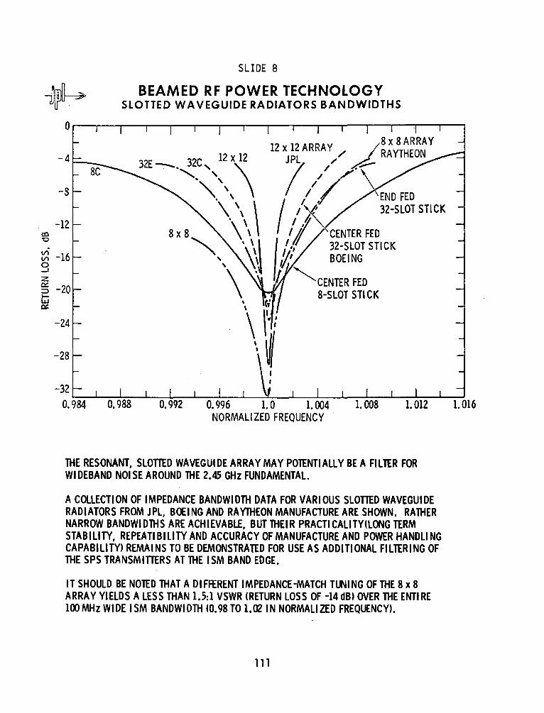
-s

-12

SLIDE 8

BEAMED RF POWER TECHNOLOGY SLOTTED WAVEGUIDE RADIATORS BANDWIDTHS

8 x 8ARRAY 12 x 12 ARRAY / I RAYTHEON

32E--.~c, 12xl2 JPL // ~

-~\\ I l/ >ENO FED \ \ \ I /~ 32-SLDT STICK

8 x 8 \ \ /I CENTER FED

~ -16 g

"' \\ \ l "'' 32-SLOT STICK ', ~ \ \~ ,'/,~ BOEING

\ • . ~CENTER FED z

0:: :::> -20 8-SLOT STICK j:;:j 0:::

-24

-28

\ ,.

\ 1•:;

\ ~ -32

.___._~..____._~_....___._~_.____.~__,___."--_._~..__----~-----~----

0. 984 0. 988 0. 992 0. 996 1. 0 1. 004 1. 008 1. 012 1. 016 NORMAL! ZED FREQUENCY

THE RESONANT, SLOTTED WAVEGUIDE ARRAY MAY POTENTIALLY BE A FILTER FOR WI DE BAND NOi SE AROUND THE 2.45 GHz FUNDAMENTAL.

A COLLECTION OF IMPEDANCE BANDWIDTH DATA FOR VARIOUS SLOTTED WAVEGUIDE RADIATORS FROM JPL, BOEING AND RAYTHEON MANUFACTURE ARE SHOWN. RATHER NARROW BANDWIDTHS ARE ACHIEVABLE, BUT THEIR PRACTICALITY(LONG TERM STABILITY, REPEATIBILITY AND ACCURACY OF MANUFACTURE AND POWER HANDLING CAPABILITY) REMAINS TO BE DEMONSTRATED FOR USE AS ADDITIONAL FILTERING OF THE SPS TRANSMITTERS AT THE I SM BAND EDGE.

IT SHOULD BE NOTED THAT A DIFFERENT IMPEDANCE-MATCH TUNING OF THE 8 x 8 ARRAY YIELDS A LESS THAN 1.5:1 VSWR (RETURN LOSS OF -14 dB) OVER THE ENTIRE 100 MHz WI DE I SM BANDWIDTH (0. 98 TO 1.02 IN NORMAL! ZED FREQUENCY).

111

SLIDE 9

BEAMED RF POWER TECHNOLOGY BEAM FORMING ARRAY PATTERNS

FLEXIBLE SUPPORT STRUCTURE

nw "'-'w

ANECHOIC CHAMBER ANTENNA RANGE

- TYPICAL SUBARRAY RECEIVER-TRANS Ml TIER UNIT

~~ '\vy POSITIONABLE

PILOT TRANSMITIER

MONOPULSE "POWER" BEAM RECEIVERS

A CONCEPT DRAWING FOR THE PILOT-BEAM-STEERED, RETRODIRECTIVE ARRAY CURRENTLY UNDER CONSTRUCTION AT JPL IS SHOWN.

BEAM POINTING ACCURACY AND OTHER ARRAY PERFORMANCE CHARACTERISTICS AS A FUNCTION OF VARIOUS PARAMETERS SUCH AS PILOT SIGNAL-TO-NOi SE RATIO AND INTERCONNECTING CABLE LENGTHS WILL BE MEASURED. BEAM FORMING PRECISION AND SI DELOBE LEVELS WILL BE DETERMINED ALONG WITH MEASUREMENT OF THE PHASE REFERENCE DISTRIBUTION AND PHASE CONJUGATION PERFORMANCE.

EACH SUBARRAY RECEIVER-TRANSMITTER UNIT WILL EMPLOY A 64-SLOT WAVEGUIDE SUBARRAY ANTENNA DI PLEXED TO BOTH RECEIVE THE PILOT SIGNALS AND TO TRANSMIT A LOW POWER SIGNAL REPRESENTING THE POWER BEAM.

AN ANECHOIC CHAMBER ANTENNA RANGE IS USED TO MINIMIZE MULTI PATH REFLECTION~ AND TO REDUCE ENVIRONMENTAL PROTECT! ON COSTS FOR THE EQUIPMENT IN THESE VER I Fl CATI ON TESTS.

112

SLIDE 10

BEAMED RF POWER TECHNOLOGY 8-ELEMENT ARA MILESTONE CHART

FY 79 FY 80 i\'.AJOR MILESTONES

AIMIJIJIAIS 0 1 NI DI JI FI Ml A I Ml JI JI" I 5

J 5ENCH TEST 2-ELEMENT ARA WITH I PrlASE REFERENCE REGENERATOR -.7

~EJESIGN e. REWO:::K ~

ALL SUSARMYS BUILT & TESTED ---.:v

?iLOT SOURCE BUILT & TESTED -7

INSTALL AR.A. IN ANECHOIC CHAMBE" ~

'iEST ARA IN ANECHOIC CHAM!lER

THE REVI SEO ACTIVE RETROD I RECTIVE ARRAY (ARA) SCHEDULE IS SHOWN. DIFFICULT CIRCUIT DESIGN FOR THE REQUIRED PHASE PRECISION, SLOW EQUIPMENT DELIVERIES AND RAPIDLY INFLATION OF EQUIPMENT COSTS HAVE CONTRIBUTED TO SCHEDULE SU PPAGE PAST THE BEGINNING OF FY '80.

113

v

CENTRAL NODE ASS'(

SLIDE 11

BEAMED RF POWER TECHNOLOGY 8-ELEMENT EXPERIMENT AL ACTIVE

RETRODIRECTIVE ARRAY (ARA) BLOCK DIAGRAM

l - - - - - - ~ TRANSMISSION LINE, TYP I i.pc

I I I t-+-~~-'---.

I I L

2. 3. 4. 5. 6. 7.

LEGEND: R-T • RCVR-XMTR-DIPLEXER ASSY .Pc• PHASE CONJUGATOR .PRR• PHASE REFERENCE REGENERATOR lfJ0 • REFERENCE PHASE 2PLX • DIPLEXER

THE OVERALL BLOCK DI AGRAM OF THE ARA IS SHOWN ALONG WITH THE DI PLEXED PILOT SIGNALS TRANSMITTER.

114

s.

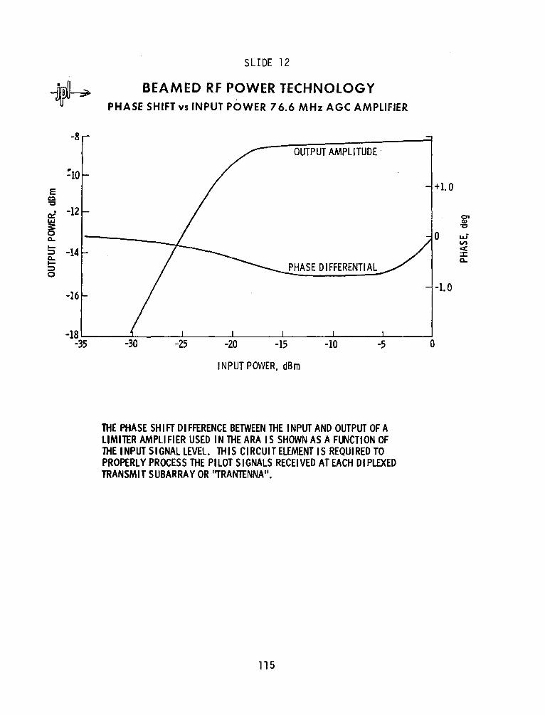
SLIDE 12

~ BEAMED RF POWER TECHNOLOGY PHASE SHIFT vs INPUT POWER 7 6.6 MHz AGC AMPLIFIER

-8

OUTPUT AMPLITUDE

=10

E c::i "O

oi -12

~ c..

!:; -14 c.. I- PHASE DIFFERENTIAL :::> 0

-16

-18 ___ _._ __ _..._ __ _...._ ___ ..___ __ _._ _____ _ -35 -30 -25 -20 -15 -10 -5

INPUT POWER, dBm

THE PHASE SHIFT DIFFERENCE BETWEEN THE INPUT AND OUTPUT OF A LIMITER AMPLIFIER USED IN THE ARA IS SHOWN AS A FUNCTION OF THE INPUT SIGNAL LEVEL. THIS CIRCUIT ELEMENT IS REQUIRED TO PROPERLY PROCESS THE PILOT SIGNALS RECEIVED AT EACH DI PLEXED TRANSMIT SUBARRAY OR ''TRANTENNA".

115

0

+1.0

C7' Cl> "O

0 LU" !on <( :I: a..

-1.0

SLIDE 13

BEAMED RF POWER TECHNOLOGY RECTENNA PATTERNS

ILLUMINATING HORN

L 0 N G A I X T I u s D

ANECHOIC CHAMBER

s ? z..

2450 MHZ

FUN DAM ENT AL & HAR1'V10N IC RECEIVING ANTENNAS

/RF GENERATOR ~~&dcLOAO

FEED LINE ~~~~

IN ORDER TO CHARACTERIZE THE EXTIRNAL ELECTRO\\AGNETIC RADIATION PERFORMANCE OF THE RECEIVING OR 11RECTINNA 11 END OF THE SPS MICROWAVE SUBSYSTIM, THE EQUIPMENT ARRANGEMENT FOR RECORDING SCATTIRED FUNDAMENTAL AND EMITTID HARMONICS FROM A SMALL, 42-D I POLE ELEMENT RECTINNA S UBARRA Y I S SHOWN.

116

RESISTOR

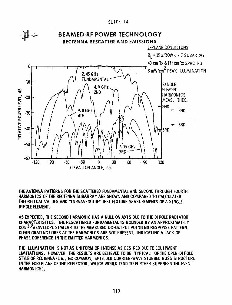
SLIDE 14

BEAMED·RF POWER TECHNOLOGY RECTENNA RESCATTER AND EMISSIONS

E-PLANE CONDITIONS

RL • 15n/ROW 6 x 7 SUBAR~AY

O 40 cm Tx & 174cmRxSPAC ING r-r--r---...,.....--..~__,,.....,..:;;:::._.-_,...,.----,.---.... 8 mW /cm2 PEAK I LLUM I NAT I ON

-10

2. 45 GHz FUNDAMENTAL ---

(\ 4.9 GHz......._ rvl I 2ND r. f20 W \ /,. I . i _30 ,-<:~GHz']! J ,~('1~ '\ L&J I \ /, I' ~ -40 v· , //'I "'\/)0tvAi' ,\ t. r~ . ~'\ \ .\ ~ I 'y/ \ I \ - Ii ~ ~ 1l\1 ,, I I \ \

\ \I ~ ~ ~I \ ~f\. ~ II ' '

SINGLE ELEMENT HARMONICS MEAS. IfilQ. 2ND

- 2ND

_. 3RD 3RD

-so rJ, / , j v~1 v fV\ , \~ r 1.35GH'z , \A I I ' H ! I~ I I 3RD --- I v l

-ro .......... ___ ._._ _ _._ _ _.__....1-J'-'-'----lL~--'----1-L-...:...L-1

-120 -90 -60 -30 0 30 60 90 120 ELEVATION ANGLE, deg

THE ANTENNA PATTERNS FOR THE SCAmRED FUNDAMENTAL AND SECOND THROUGH FOURTH HARMON I CS OF THE RECTENNA SU BARRA Y ARE SHOWN AND COMPARED TO CALCULATED lHEORETICAL VALUES AND "IN-WAVEGUIDE" TEST FIXTURE MEASUREMENTS OF A SINGLE DI POLE ELEMENT.

AS EXPECTED, THE SECOND HARMONIC HAS A NULL ON AXIS DUE TO THE DIPOLE RADIATOR CHARAiTERISTICS. THE RESCAmRED FUNDAMENTAL IS BOUNDED BY AN APPROXIMATELY COS 1. eENVELOPE SIMILAR TO THE MEASURED DC-OUTPUT POINTING RESPONSE PATTERN. CLEAN GRATING LOBES AT THE HARMONICS ARE NOT PRESENT, INDICATING A LACK OF PHASE COHERENCE IN THE EMITTED HARMONICS.

lHE ILLUMINATION IS NOT AS UNIFORM OR INTENSE AS DESIRED DUE TO EQUIPMENT UMITATIONS. HOWEVER, THE RESULTS ARE BELIEVED TO BE ''TYPICAL" OF THE OPEN-DI POLE STYLE OF RECTENNA O.e., NO COMMON, SHIELDED QUARTER-WAVE STUBBED BUSS STRUCTURE IN THE FOREPLANE OF THE REFLECTOR, WHICH WOULD TEND TO FURTHER SUPPRESS THE EVEN HARMON I CS ).

117

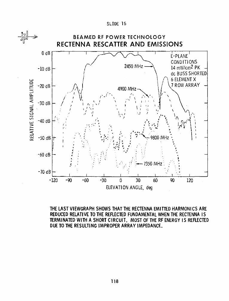
LI..J c::i

0 dB

-10 dB

SLIDE 15

BEAMED RF POWER TECHNOLOGY

RECTENNA RESCATTER AND EMISSIONS

"' ~ E-PLANE ~ /

2 \ CONDITIONS

/ - 450 MHz - 14 mW/cm2 PK ! \ "' de BUSS SHORTED

~ -20 dB I I / \ 6 ELEMENT x

, ,.;\) (-, 4900 M_Hz~ \ {- {ROW ARRAY -I a.. ~

:S -30 dB / ,' V, ,, ,i·· \ ,,,,.-_, :·· . . -', ~I \ \

: \ ,\ : " : : \ i '.,: I, : ' \ <( z <..::> . / : , '1 •\ I : I ,t \ I -.

I J •• ,( \I' ,., ~ -40 dB ... I

' .' • / • \, •f\ 1·• I < • < J ( \ . 1' fl("'{ '1

• "• : • ... " .... ~ I ( ( .( rt._ ~ 'J '"' v l > i \

1-,.

,. ,. : It~· ~ ., •.

:5 ~ -50 dB i

'( . ·" ., ,,, '( ~ .. ., "' • • • 1' • \ '

;' · .. { .. '.(.: .~ ;·· . •: ·~9800 MHz.'. : ,. • .. . ., ,. ; > r/ ')

-60 dB

-70 dB

' ' ( . ' ~ . ' . . '

.. •• I ... . . .

'•

.. . '

' ·'

I ;. II>. > 41 0

p . {·,.: "' ( .· ·. . ',. c,:(< ''• ~ ' . . ..

.. : .· ·: . .-·" .· : ~: ".:.__ 7350 MHz ~-·.: :: . I

. ~ . . .

' . )

. . .. ... ~~-'-~--'-~~-L-~---1.-~~~~--J-~~L..._~-'-~--'

-120 -90 -60 -30 0 30 60 90 120 ELEVA Tl ON ANGLE, dE-g

THE LAST VIEWGRAPH SHOWS THAT THE RECTENNA EMlffiD HARMON I CS ARE REDUCED RELATIVE TO THE REFLECTED FUNDAMENTAL WHEN THE RECTENNA IS TERMINATED WITH A SHORT CIRCUIT. MOST OF THE RF ENERGY IS REFLECTED DUE TO THE RESULTING IMPROPER ARRAY IMPEDANCE.

118

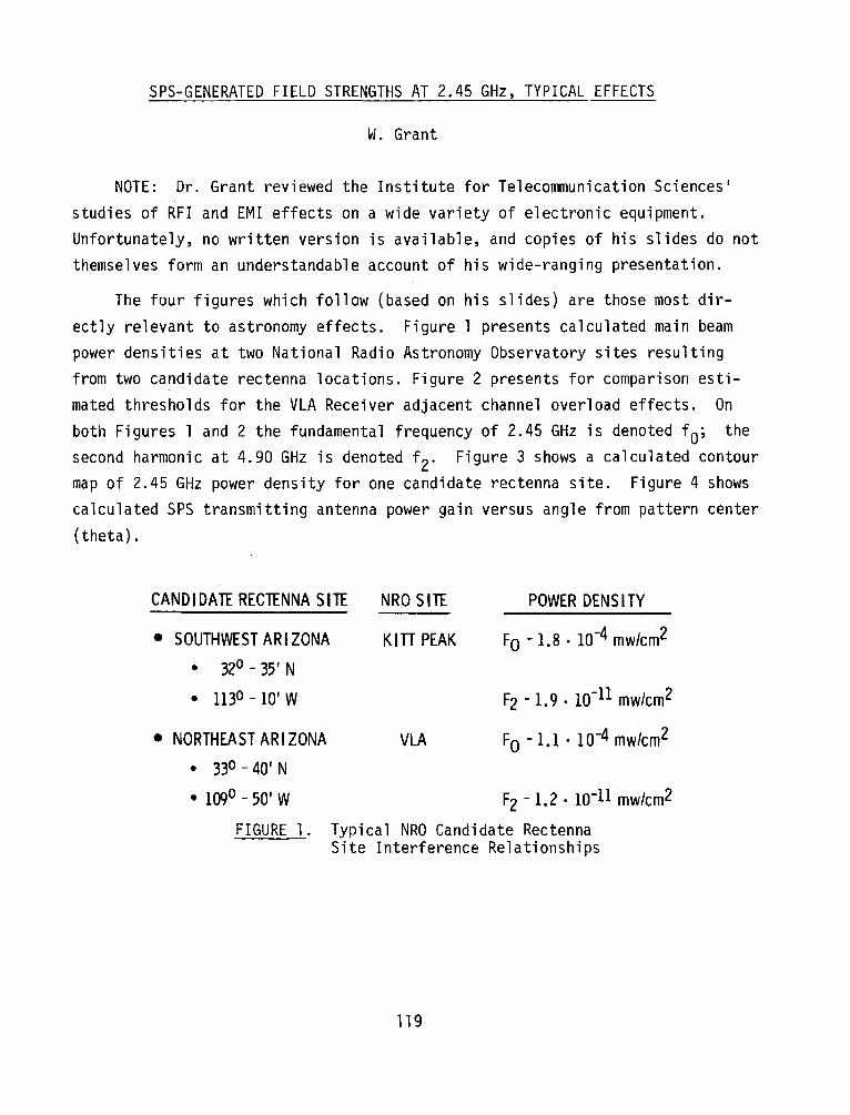
SPS-GENERATED FIELD STRENGTHS AT 2.45 GHz, TYPICAL EFFECTS

W. Grant

NOTE: Dr. Grant reviewed the Institute for Telecommunication Sciences'

studies of RFI and EMI effects on a wide variety of electronic equipment. Unfortunately, no written version is available, and copies of his slides do not themselves form an understandable account of his wide-ranging presentation.

The four figures which follow (based on his slides) are those most dir­

ectly relevant to astronomy effects. Figure l presents calculated main beam power densities at two National Radio Astronomy Observatory sites resulting from two candidate rectenna locations. Figure 2 presents for comparison esti­mated thresholds for the VLA Receiver adjacent channel overload effects. On both Figures l and 2 the fundamental frequency of 2.45 GHz is denoted f 0; the second harmonic at 4.90 GHz is denoted f 2. Figure 3 shows a calculated contour map of 2.45 GHz power density for one candidate rectenna site. Figure 4 shows calculated SPS transmitting antenna power gain versus angle from pattern center

(theta).

CANDI DAlE REClENNA S llE

• SOUTHWEST ARI ZONA

• 32° - 35 1 N

• 1130 -10' w

• NORTHEAST AR I ZONA

• 33o - 40' N

NRO SllE

KITT PEAK

VLA

POWER DENSITY

Fo - 1.8 • 10-4 mw/cm2

F2 - 1. 9 • 10-ll mw/cm2

Fo - 1.1 • 10-4 mw/cm2

• 109° - 50' W F2 - 1.2 • 10-11 mw/cm2

FIGURE 1. Typical NRO Candidate Rectenna Site Interference Relationships

119

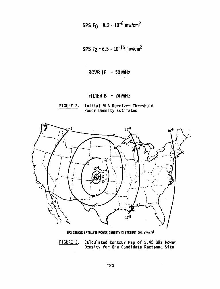
SPS Fo - 8.2 • io-6 mw/cm2

SPS F2 - 6.5. io-16 mw/cm2

RCVR IF - 50 MHz

FILTER B - 24 MHz

FIGURE 2. Initial VLA Receiver Threshold Power Density Estimates

SPS SINGlf SAlE.lllTE POWER DENSITY DISTRIBUTION, mw/cm2

FIGURE 3. Calculated Contour Map of 2.45 GHz Power Density for One Candidate Rectenna Site

120

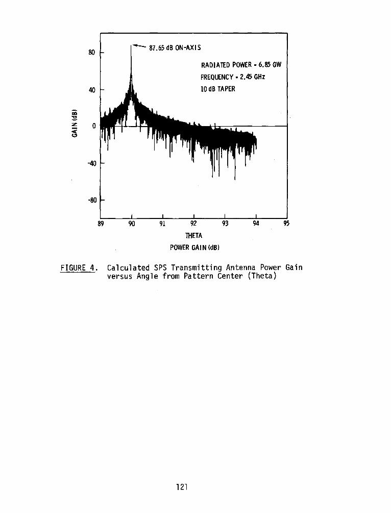
80

40

z 0

-80

89

.__ 87.65 dB ON-AXIS

90 91

RADIATED POWER • 6.85 GW

FREQUENCY • 2.45 GHz

10 dB TAPER

92

lllETA

POWER GAi N (dB}

93 94 95

FIGURE 4. Calculated SPS Transmitting Antenna Power Gain versus Angle from Pattern Center (Theta)

121

INTERFERENCE EFFECTS ON RADIO ASTRONOMY EQUIPMENT

W. C. Erickson

The principal interference effects of the proposed SPS on radio astronomi­cal observations have been discussed in the Briefing Document and in the Committee on Radio Frequencies/National Academy of Sciences (CORF/NAS) assess­ment. I will amplify on these assessments.

Radio astronomy is particularly sensitive to interference. Because we typically detect signal levels of lo-18 to lo- 21 W, we are sensitive to very low levels of interference. For this reason, radio astronomers have success­fully endeavored to obtain protection from interference by active users of the radio spectrum. Radio astronomy has been established as a Radio Service in the frequency management community and has been granted protection from interfer­ence by the other Services. The degree of this protection varies from band to band depending on our needs and those of the other Services.

In order to provide standards which can be used in the design of systems trat might interfere with radio astronomy observations, it is necessary to state a formal definition of "harmful interference" to radio astronomy. This has been done by the CCIR Report-224 which was first issued in 1963 and has been occasionally updated, the most recent issue--CCIR Report 224-4--having been adopted by the 1978 Kyoto KIV Plenary Assembly (cf Appendix A). This definition of "harmful interference" has changed little over the years and has proven to be a remarkably accurate statement of our needs.

The relevant standards for continuum bands are:

Frequency (GHz)

1.4

2.5

5

10

15

Power Flux Spectral Density dB (w/m2-Hz)

-255

-247 -241 -240

-233

123

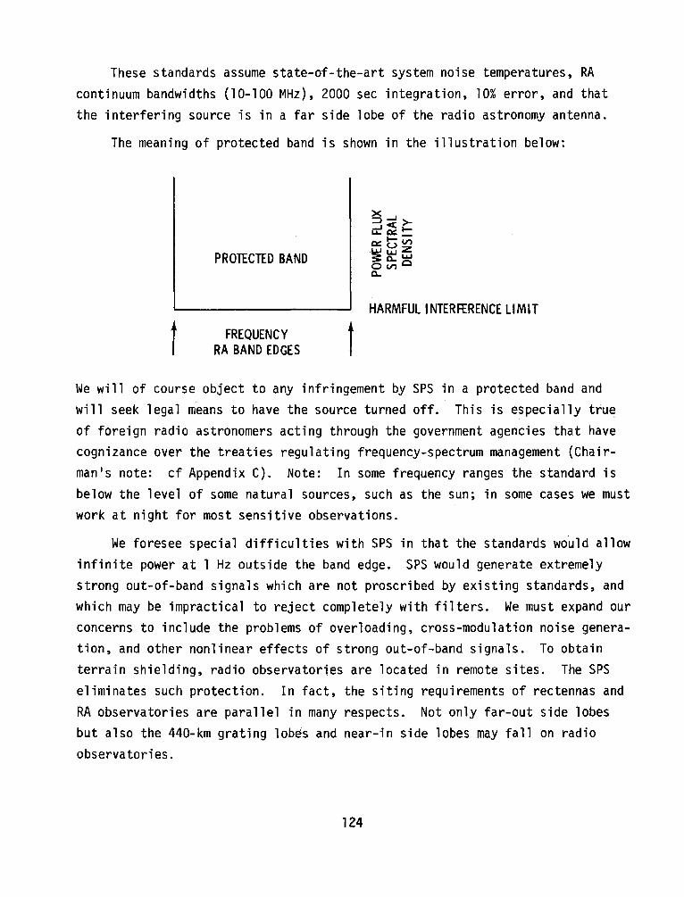
These standards assume state-of-the-art system noise temperatures, RA continuum bandwidths (10-100 MHz), 2000 sec integration, 10% error, and that the interfering source is in a far side lobe of the radio astronomy antenna.

The meaning of protected band is shown in the illustration below:

t

PROTECTED BAND

FREQUENCY RA BAND EDGES

HARMFUL INTERFERENCE LIMIT

t We will of course object to any infringement by SPS in a protected band and will seek legal means to have the source turned off. This is especially true of foreign radio astronomers acting through the government agencies that have cognizance over the treaties regulating frequency-spectrum management (Chair­man's note: cf Appendix C). Note: In some frequency ranges the standard is below the level of some natural sources, such as the sun; in some cases we must work at night for most sensitive observations.

We foresee special difficulties with SPS in that the standards would allow infinite power at l Hz outside the band edge. SPS would generate extremely strong out-of-band signals which are not proscribed by existing standards, and which may be impractical to reject completely with filters. We must expand our concerns to include the problems of overloading, cross-modulation noise genera­tion, and other nonlinear effects of strong out-of-band signals. To obtain terrain shielding, radio observatories are located in remote sites. The SPS eliminates such protection. In fact, the siting requirements of rectennas and RA observatories are parallel in many respects. Not only far-out side lobes but also the 440-km grating lobes and near-in side lobes may fall on radio observatories.

124

The seriousness of the problem is indicated by the following:

• Within a 30-MHz RA band at 2.7 GHz, -255 dB(w/m2 Hz) implies total noise emission of 15 mW by an isotropic radiator at a distance of 35800 km. In any 3-kHz band 1.5 µW would exceed the standard. If a sub-array gain of 50 dB is assumed, numbers are decreased by 105. 6· 7 GW implies 156-dB l. 5 µW reduction in signal level from 2.45 GHz to 2.67 GHz or 206-dB reduction if sub-array gain is considered.

• For the case of 100 satellites, an additional 20 dB is required.

Depending on transmitter amplifier and antenna design, this level of performance is at least conceivable. However, reliability of transmitter subsystems would be extremely critical. Each satellite has 105 x 70-KW klystrons. One of these devices developing some subtle error to radiate ~ l µW in an RA band will exceed standards. It may prove to be extremely difficult to locate and turn off the offending unit.

The potential overloading problems are severe. The projected power levels '\., '\., 2

at 2.45 GHz for ("' l Earth radius) from the SPS main beam are - 2 µW/m . This is equivalent to the power level from a 10-kw transmitter with gain of 20 located 100 km from observatory, line-of-sight. A large telescope with ~ 40-dB side lobes would produce"' l µW from such a source. Parametric amplifiers give trouble at about 0.001 µW. System performance may be seriously degraded by one satellite at 2.45 GHz, but good filters might handle the problem. It is interesting to note that a 100-satellite system is equivalent to a 10-kW transmitter at 10 km from the observatory. A 440-km side lobe is equivalent to a transmitter at 1.4 km from the observatory. It does not appear to be possible for a radio observatory to operate within a few hundred kilo­meters of a rectenna. This problem needs much more study.

Other effects of interference require investigation, including:

• Ionospheric Modification: What of scattering at 2.45 GHz? What of reflection of terrestrial interference by modified ionosphere? What of ionospheric cross-modulatior effects,? What of large-scale ionospheric modification?

125

• Rectenna Scattering: If 2% of incident power is scattered, the rectenna forms a 120-MW transmitter at 2.45 GHz.

• Harmonic Emission: RA Band .

2nd Harmonic at 4.90 GHz 4.95-5.0 Formaldehyde at 4.829 GHz

4th Harmonic at 9.80 GHz 10. 6-10. 7 GHz 9th Harmonic at 22.05 GHz 22.21-22.5

H20 at 22.235 GHz

• Thermal Noise: Thermal emission from sps· could interfere with many observations.

•·Test Systems: Initial, low-power tests of components of the SPS could seriously damage radio astronomy observations.

126

POSSIBLE OVERLOAD AND PHYSICAL DAMAGE OF A RADIO ASTRONOMY RECEIVER CAUSED BY THE SPS

H. Hvatum

The extremely high microwave power radiated from the SPS (several orders of magnitude higher than any other existing or planned microwave transmitter) raises the question of overload problems and, perhaps, physical damage to radio astronomy receivers. It is therefore of interest to estimate the power levels in a radio astronomy receiver under various conditions that might arise.

One may safely assume that the main beam of the SPS will always be dir­ected towards a rectenna and that in case of equipment failure the beam will degenerate into the phase failure mode. Thus, a radio astronomy receiver will never be exposed to a SPS main beam, but will be illuminated either by the SPS side lobe structure or the phase failure mode radiation. If one assumes that a complete SPS consists of approximately 100 SPS sets (60 and 120 sets have been mentioned), the average distance between two adjacent rectennas will be about 300 km. Thus, a radio astronomy installation will, on the average, be withi~ a few hundred kilometers from a rectenna and be illuminated with about 3 mW/m2 from one SPS transmitter. With 100 systems in operation, the flux will be higher, although not 100 times higher since the contribution from most systems will come from far-out side lobes.

A combined flux of 50 to 100 mW/m2 seems to be a reasonable estimate of the combined power flux that could be expected from all SPS transmitters. With 100 SPS transmitters in simultaneous operation, it becomes quite likely that a grating lobe with a power flux of 100 mW/m2 will fall on a radio astronomy telescope. In the following calculations, 100 mW/m2 has been used as a typical expected power flux at a radio astronomy observatory.

The interfering radiation will be coupled into the radio astronomy receivers either through the side lobes of the radio telescope or occasionally through the main beam. Both cases must be considered.

127

Under normal operation the radiation from the SPS transmitter will couple into the side lobes of the radio telescope. The side lobe response of a radio astronomy telescope is independent of its size, about 7 dB below the isotropic response.

The SPS satellites will be in geosynchronous orbits, which means that they will occupy a band across the United States near the celestial equator, a region of great interest to radio astronomy. One must assume that the main beam of a radio telescope accidentally may point at one of the SPS transmitters. For a 25-m-diameter telescope the gain is about 54 dB at 2.4 GHz, which gives about 61 dB higher power level in the input amplifier compared to the case where the antenna is pointed away from the satellite.

In the case of an SPS transmitter operating in the phase failure mode, the radiated beam becomes very wide and will cover the entire United States. The power flux from one SPS will then be 30 mW/m2 anywhere.

A typical radio astronomy system uses parametric amplifiers as low-noise input stages. The overload level, defined here as a 0.1-dB compression in the amplifier, is about 3 x 10-9 Wand the level where the varactor may be physically damaged (burn-out) is about 100 mW.

In order to achieve the best possible system noise temperature, a normal radio astronomy receiving system does not employ filters in front of the input amplifer. Thus, a system operating in the 2690 to 2700 MHz radio astronomy band will also be exposed to fields at 2450 MHz, the SPS frequency.

The rectennas will reradiate 5% of the incoming power, or about 100 MW. Most of the reradiated power will be at 2.45 GHz, but some (-25 dB) will occur at 4.9 GHz. If one assumes that the reradiation will be isotropic, at a dis­tance of 150 km the power flux will then be approximately 5µW/m2.

One can now assume the following parameters for the SPS-radio astronomy system:

128

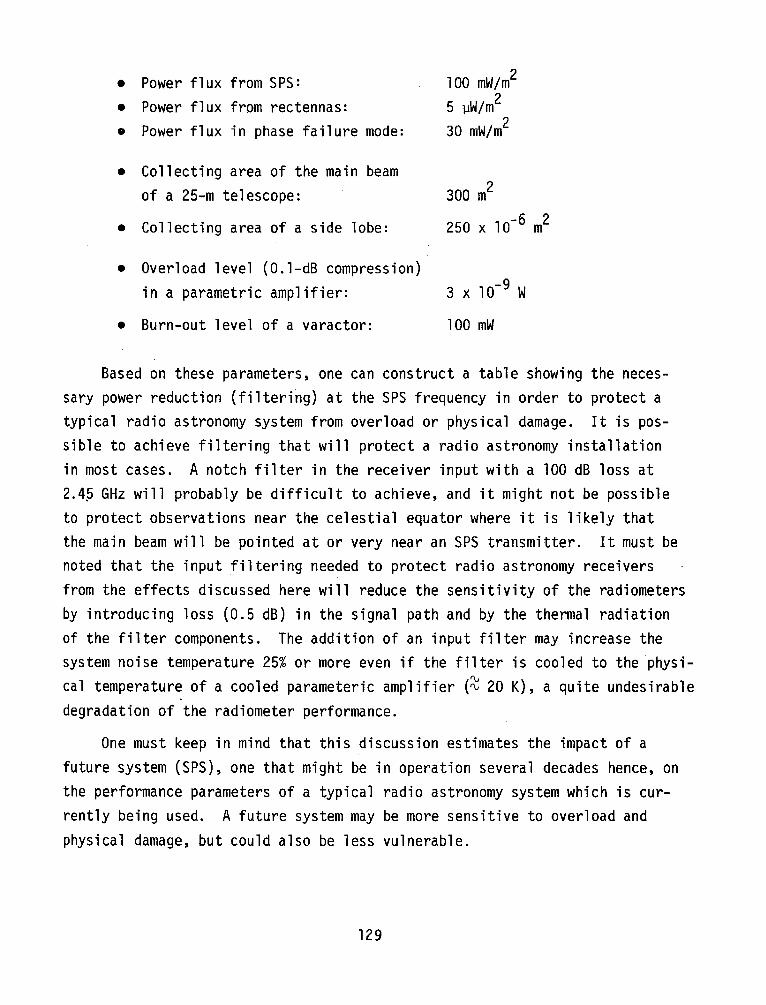
• Power flux from SPS: • Power flux from rectennas: • Power flux in phase failure mode:

• Collecting area of the main beam of a 25-m telescope:

• Collecting area of a side lobe:

• Overload level (0.1-dB compression) in a parametric amplifier:

• Burn-out level of a varactor:

100 mW/m2

5 µW/m2

30 mW/m2

300 m2

250 x 10-6 m2

3 x 10-9 w

100 mW

Based on these parameters, one can construct a table showing the neces­sary power reduction (filtering) at the SPS frequency in order to protect a typical radio astronomy system from overload or physical damage. It is pos­sible to achieve filtering that will protect a radio astronomy installation in most cases. A notch filter in the receiver input with a 100 dB loss at 2.4p GHz will probably be difficult to achieve, and it might not be possible to protect observations near the celestial equator where it is likely that the main beam will be pointed at or very near an SPS transmitter. It must be noted that the input filtering needed to protect radio astronomy receivers from the effects discussed here will reduce the sensitivity of the radiometers by introducing loss (0.5 dB) in the signal path and by the thermal radiation of the filter components. The addition of an input filter may increase the system noise temperature 25% or more even if the filter is cooled to the physi­cal temperature of a cooled parameteric amplifier (~ 20 K), a quite undesirable degradation of the radiometer performance.

One must keep in mind that this discussion estimates the impact of a future system (SPS), one that might be in operation several decades hence, on the performance parameters of a typical radio astronomy system which is cur­rently being used. A future system may be more sensitive to overload and physical damage, but could also be less vulnerable.

129

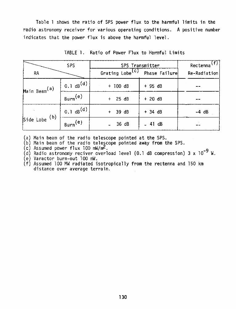
Table 1 shows the ratio of SPS power flux to the harmful limits in the radio astronomy receiver for various operating conditions. A positive number indicates that the power flux is above the harmful level.

TABLE 1. Ratio of Power Flux to Harmful Limits

~ SPS Transmitter Rectenna(f)

A Grating Lobe(c) Phase Failure Re-Radiation

~~a in Beam( a) 0.1 dB(d) + 100 dB + 95 dB --

,,

Burn(e) + 25 dB + 20 dB --

0.1 dB(d) + 39 dB + 34 dB -4 dB Side Lobe (b) -·

Burn{e) - 36 dB - 41 dB --

(a) Main beam of the radio telescope pointed at the SPS. (b) Main beam of the radio telescope pointed away from the SPS. (c) Assumed power flux 100 mW/m2. (d) Radio astronomy reciver overload level (0.1 dB compression) 3 x 10-9 W. (e) Varactor burn-out 100 mW. (f) Assumed 100 MW radiated isotropically from the rectenna and 150 km

distance over average terrain.

130

-

POTENTIAL IMPACT OF OUT-OF-BAND RADIATION FROM THE SATELLITE POWER SYSTEM

AT ARECIBO OBSERVATORY

M. M. Davis

Arecibo Observatory, operated as a national research center by Cornell University, has the world's largest radio/radar telescope. Its S-band radar system at 2380 MHz is the source of the most powerful collimated signal leaving the Earth; at the same time, its 20-acre collecting area and maser receivers provide the highest instantaneous sensitivity anywhere for the reception of faint signals. The observatory carries out a wide range of research in astronomy, planetary radar and atmospheric physics over its usable frequency range of 5 to 5000 MHz. In addition, an active optical program of airglow research is underway as part of the atmospheric physics program.

All of these programs could be severely affected by out-of-band radiation or optical scattering from the satellite power system. The harmful interfer­ence levels for radio astronomy in the protected frequency bands are adequately covered by the discussion and tables in CCIR 224-4. It should be noted, however, that these tables are based on an isotropic side lobe level, and assume that the main beam and near-in side lobes are pointed well away from the interfering source. At Arecibo, the available sky coverage is limited to a maximum of 20° zenith angle. The relationship between the Arecibo coverage and the power satellite locations is shown in Figure 1. The figure makes clear that at southern declinations the beam must necessarily come close to the power satellites. In general, the need to accurately correct for spherical aberra­tion has as a byproduct a remarkably 11 clean 11 beam pattern at Arecibo, but it is nevertheless clear. that the sensitivity at southern declinations may be par­ticularly affected by SPS out-of-band radiation.

Three areas are of particular concern at Arecibo: second harmonic radia­tion, the effect on the planetary radar system at 2380 MHz, and the impact on airglow observations. Second harmonic SPS radiation is of special concern at Arecibo because it falls in our highest frequency band. The Arecibo reflector

131

D EC (degrees I 36 ....t::

34 ~ JA/

32 ,£ YI"'

30~ f

il1 1/. 28 ..l..LJ

26 'JLL//

_,Ur I

4 l.J II

Ji... J 'J...1:.t

2

22 20

18

16

14

J..J

I

. -

2 l.! _\ 10 li

\: j.

8 ~ \: '' "\.

6 ~ ~ ' 4 ~' '\.

2 '" ...... ~ ....

38 .; ,..._i. 'f. v

0 - .~,.... ..... ...... ......

ARECIBO SKY COVERAGE

-~

FIGURE 1.

0 10 20 30 - 40 LHA (ml .... 50 .... .... ";~60 ""' ::-..1. ,, ,,. 70

~ .::ii

' " .,,,. ~~o

:I.I '~ \

I\

1.111

lj LJ 80 11

IL 1/ v

ILJ v :... 70 ,, I'/

/

/ /V/ 60 " ...... _::. '/ 50 ......

...... 40 30

20 SOLAR POWER S o.J~••••••••••••••••••

ATELLITES .. Arecibo Sky Coverage

was upgraded recently to provide high sensitivity and resolving power (1 'FWHM) in the protected band at 5 GHz, and any radiation in this band above the harm­ful interference limits of CCIR 224-4 will degrade or eliminate the Arecibo 6-cm research.

The second concern is not directly addressed by CCIR 224-4, as it involves planetary radar. The 430-kw Arecibo cw radar operates ·on an assigned frequency of 2380 MHz. The receiver is a Jet Propulsion Laboratory maser. The normal observing mode involves transmitting for periods ranging from a few to tens of minutes in order to fill the round-trip travel time window between the earth and the target planet, satellite, or asteroid. A reception period of equal duration then follows. The bandwidth used during reception is set by the nature of the target and range~ from 0.02 Hz for Venus at conjunction to 30 kHz for Saturn's rings. The harmful interference level calculated for these band­widths, but otherwise using the same criteria as CCIR 224-4, ranges from -204 to -235 dbW/m2-Hz. The latter figure, which applies to "soft" targets

132

such as Saturn's rings, is similar to the values derived in CCIR 224-4 for spectral line radio astronomy in this wavelength region. If the SPS noise power density can in fact be limited to that shown in Figure 26 of Satellite Power System: System Report, DOE/ER - 0023, October 1978, then the noise from 60 power satellites lies at the harmful interference threshold for planetary radar research.

The third area of particular concern to Arecibo is the impact of direct and scattered su~light on airglow research. Because of the weakness of most (non-auroral) airglow emission features, airglow observing is traditionally a 11 dark moon 11 activity. It is almost impossible to obtain useful measurements with direct moonlight in the field of view of an instrument. In fact, mahy automatic photometers incorporate protection devices to guard against possible detector damage caused by exposure to direct moonlight. In investigations of spatial variations, north-south meridian scanning is a corrunon mode of opera­tion. A chain of satellites across a meridian could seriously limit studies of the dynamic behavior of the airglow.

The problem of moonlight scattered into the field of view is rather dif­ficult to quantify, as it depends on local tropospheric conditions. Adequate measurements of strong emission features can probably be obtained when the moon is less than 1/4 full. However, recent developments on instrument design and detector technology have made it possible to observe very weak airglow features. Work of this type is seriously compromised by an increase in background bright­ness by a factor of 5, such as is caused by the presence of the Milky Way in the fiel9 of view. At Arecibo, an increase in sky brightness of this order is observed at the zenith when a moon about 1/8 full {by area) is present near the horizon. Scattered light from the SPS of this amount would seriously compro­mise present airglow research at Arecibo.

The discussion has thus far assumed that a rectenna array is not placed in Puerto Rico. In fact, the extrapolated power requirements in Puerto Rico match the 5-GW capability of an SPS, and the island imports 100% of its energy. For these and other reasons, it may be selected for a rectenna site early in the program. If it is selected, the interference criteria may be much more dif­ficult to meet, both because the observatory will lie in the near-pattern of

133

the transmitting array and because rectenna scattering and noise generation will have to be taken into account. Such effects will require careful study if the observatory's research is not to be unnecessarily affected.

This discussion is based on current operations at the Arecibo Observatory. The present 1000-ft telescope is a general-purpose instrument with enormous pressure for observing time from its widely-diversified user community. There are at present no plans to duplicate this facility; and as a unique instrument it is expected to continue in operation for many decades. Extrapolating into the future, there are plans to erect a 100-m aperture all-sky telescope, with wavelength coverage extending down to ~ l cm. The SPS therefore poses a very real threat if out-of-band radiation cannot be controlled to the required strict.thresholds stated in CCIR 224-4.

134

THE EFFECTS OF THE PROPOSED SATELLITE POWER SYSTEM ON THE VLA

A. R. Thompson

The Very Large Array (VLA) is being constructed on the Plains of San Augustin, New Mexico as a facility to map the sky at centimetre wavelengths with angular resolution down to a few tenths of an arcsecond. The array, when completed, will consist of 27 fully steerable paraboloid antennas of 25-m diameter, located on a three-armed array with nine on each arm. The antennas can be moved between foundations so that the scale of the array can be varied in four steps in which the distance of the furthest antenna from the center varies between 0.6 and 21 km. A general description of the array has been given by Heeschen (1975), and more detailed accounts can be found in NRAO technical reports.

The array operates in the Fourier Synthesis mode in which signals from all possible pairs of antennas are combined to form a two-dimensional visibility function. To obtain sufficient data the point in the sky being observed is usually tracked over a range of at least -4 to +4 hours in hour angle. The sky brightness function is then obtained from the visibility by Fourier transforma­tion. For an account of the principles involved see, for example, Swenson and Mathur (1968) or Fomalont and Wright (1974).

Table l gives the four wavelength bands in which the VLA is equipped to operate at the present time. Each of these VLA bands encompasses a narrower band assigned to radio astronomy. Note that harmonics of the SPS frequency at 4.9, 14.7 and 22.05 GHz fall within VLA operating bands. The receiving equip­ment is capable of operation with an instantaneous bandwidth of up to 100 MHz in two orthogonal polarizations. Bandwidths wider than the assigned radio astronomy bands are often used, if no other signals are encountered, to maxi­mize the sensitivity.

Two effects in the operation of such an array reduce the response to

radiation from directions in the sky other than that desired. First, the unwanted source does not have the expected motion across the sky of the point

135

~

w °'

i

VLA Band Wavelength

1'340-1730 MHz j 18-21 cm I I

4500-5000 MHz ! 6 cm I '

I

I 14.4-15.4 GHz 2 cm !

22.0-24.0 GHz 1. 3 cm

I

TABLE 1. VLA Observing Bands

Minimum Detectable Signal(a) (Approximate) '

10- 30 W m- 2 Hz- 1

8 x 10- 31 W m- 2 Hz

I

Radio Astronomy Band

1400-1427 MHz

4990-5000 MHz

5 x 10- 30 W m- 2 Hz- 1 : 15.35-15.40 GHz

7 x 10- 30 W m- 2 Hz- 1 !

23.6-24.0 GHz

(a)Signal level equivalent to 5 times rms noise.

Atomic and Molecular Lines

Neutral Hydrogen 1420.4 MHz HCONH 2 (Formamide) 1538-1542 MHz OH 1612, 1665, 1667, 1721 MHz HCOOH (Formic Acid) 1639 MHz

HCONH2 (Formamide) 4617-4620 MHz OH 4660, 4751, 4766 MHz H2CO (Formaldehyde) 4830 MHz

H2CO (Formaldehyde) 14.489 GHz

H20 22.235 GHz NH3 (Ammonia} 22.835-23.870 GHz

under observation. The receiving system is set up to compensate for phase changes resulting from the expected motion, and the output from the unwanted signal becomes a quasi-sinusoidal waveform which is reduced in amplitude by time-averaging in the data processing. This effect will be referred to as fringe-frequency averaging. Second, the variable delays within the receiving system are adjusted to compensate for the difference in space transmission paths for radiation from the desired direction, but the time delays for inter­fering signals are generally unequal. If the interference is broadband, it is therefore partially decorrelated.

Calculations have been made to estimate the quantitative effects of the fringe-frequency averaging and the decorrelation. The fringe-frequency aver­aging depends on the size of the synthesized field of view, and hence on the configuration and observing frequency. The most compact configuration, for which the interference reduction is least effective, will be used in consider­ing the tolerable interference levels. For this case the reduction is approxi­mately 10 dB for the 18 to 21 cm band and 17 dB for 1.3 cm. These figures refer to declinations south of +70°, and the fring-frequency averaging becomes less effective toward the pole. The decorrelation effect depends mainly on the antenna configuration and the bandwidth, and again the most compact configura­tion will be considered. The interference reduction is approximately 17 dB for a 25-MHz bandwidth and 17 dB for a 50-MHz bandwidth. These figures apply to a source of interference at the declination of the satellite, -5.5°, and for an observing declination north of +20°. As the observing declination approaches that of the satellite, the interference reduction becomes much less effective.

Harmful interference levels, which are regarded as the general criteria for radio astronomy observations, are given in CCIR Report 224-4. These levels are derived by considering observations using a single large antenna, for which the fringe-frequency averaging and decorrelation effects do not apply. Thus, under certain circumstances, the array should be able to operate with no decrease in performance in the presence of interference levels above those indicated in CCIR Report 224-4. The CCIR levels refer to interference received

in the far side lobes of the antennas, for which the gain is equivalent to that of an isotropic radiator. With this condition, and for declinations from +20°

137

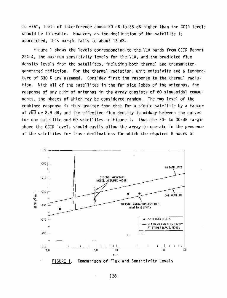
to +75°, leels of interference about 20 dB to 35 dB higher than the CCIR levels should be tolerable. However, as the declination of the satellite is approached, this margin falls to about 13 dB.

Figure l shows the ievels corresponding to the VLA bands from CCIR Report 224-4, the maximum sensitivity levels for the VLA, and the predicted flux density levels from the satellites, including both thermal and transmitter­generated radiation. For the thermal radiation, unit emissivity and a tempera­ture of 330 K are assumed. Consider first the response to the thermal radia­tion. With all of the satellites in the far side lobes of the antennas, the response of any pair of antennas in the array consists of 60 sinusoidal compo­nents, the phases of which may be considered random. The rms level of the combined response is thus greater than that for a single satellite by a factor of /60 or 8.9 dB, and the effective flux density is midway between the curves for one satellite and 60 satellites in Figure l. Thus the 20- to 30-dB margin above the CCIR levels should easily allow the array to operate in the presence of the satellites for those declinations for which the required 8 hours of

N I

":-' E 3: cc "C

-170 ..-----------------------------,

-190

-210

-230

-250

-270

290

-310 1.0

SECOND HARMON IC

iyt-NOISE, ASSUMED -40dB

1:

" " ,, ONE SATELLITE

THERMAL RADIATION ASSUMES UNIT EMISSIVITY

5.0 10

CHZ

e CC IR 224-4 LEVELS

1---i VLA BAND AND SENSITIVITY AT 5 TIMES R. M. S. NOISE

-50

FIGURE 1. Comparison of Flux and Sensitivity Levels

138

100

tracking can be achieved without presenting to the satellites an antenna response much greater than isotropic. There will be a small additional inter­ference-reducing effect resulting from the resolution of the 0.5- x 1.0-arc­minute collector arrays by the spaced antennas. This resolution effect, incidentally. enables the array to operate in the daytime in the presence of the quiet sun, which is, of course, much more highly resolved than a satellite.

Since the line of satellites is essentially constant in declination, at -5.5° as viewed from the VLA site. there will be a zone of declinations centered on -5.5° in which the array cannot operate without receiving inter­ference above a tolerable level. In this zone interference could be avoided only by reducing the range of hour angle tracking by something more than the 60° longitude range of the satellites, and satisfactory mapping of celestial objects would not be possible. At the present time the low level response of the antennas is not well enough known to define the zone with accuracy. The antennas operate in the Cassegrain mode with the feeds placed on a circle of o.g7-m radius about the vertex (Weinreb et al. lg77, Gustincic and Napier lg77). As a source of radiation moves away from the beam center, the antenna response falls sharply. but then becomes dependent on spillover of the feed response at the edge of the subreflector. The subreflector subtends an angle of 18° at the feed, and the gain of the feeds falls from 26 dB near the center of the subreflector to 13 dB at the edge. Thus, at go off axis the antenna gain is close to 13 dB,(a) and it fallsto the isotropic level at the angle at which the feed response becomes isotropic. This angle is given for each feed in Table 2. The very large angle for 18 to 21 cm results from the horn being placed 1.5 m behind the correcting lens, which provides a compact and econom­ical design, but allows some spillover at the edge of the lens. However, it should be possible, by using much more expensive feeds, to bring the side lobe performance at 18 to 21 cm much closer to that of the other feeds.

Because the tolerable interference level falls as the declination of observation approaches that of the satellites, observations with satellites in the 13 dB side lobe at the subreflector edge would be very close to the

(a) Because of the offset feed arrangement, the spillover side lobe is not precisely centered on the main beam and the go figure is the mean distance from the beam axis.

139

TABLE 2. Gain and Side Lobe Estimates for VLA Antennas

Wavelength Gain on Approximate Level of Angle at Which (cm) Main Beam Wide-Angle Side Lobes Gain is Isotropic

Relative to Main Beam

22 L 48 dB -52 dB ±44° 6 c 59 -63 ±12° 2 Ku 68 -73 ±12° 1.35 K 72 -77 ±12°

threshold of harmful interference, at least with the most compact antenna conftguration. It is also possible that scattering by subreflector supports may produce side lobes which will preclude pointing as close to the satellites as the angles in Table 2. The most that can presently be said is that for some observations, particularly those of lower angular resolution, the zone in which satisfactory mapping is precluded is probably not much less than 24° wide in declination.

It will be realized, of course, that the level of thermal radiation from a satellite is similar to the flux density of many of the stronger cosmic radio sources. The positions and flux densities of such sources are accurately known, and their responses can be calculated with precision and subtracted from maps of other objects. The satellites, however, would be expected to vary relatively rapidly in flux density and position as they maneuver to track the sun and hold their stations in orbit.

Now consider the transmitter-generated radiation, which is much more dependent on presently unknown design details than is the thermal radiation. At a few hundred km from a rectenna, the 2.45-GHz power signal from the cor­responding satell1te would be received at a level of about -60 dBW in an isotropic radiator. This is about 13 dB over the threshold for overloading of the parametric amplifiers. The 18 to 21 1cm band would require some additional . filtering, but for the other bands 2.45 GHz is below cutoff for the input wave guides. The second harmonic, for which a relative level of -40 dB will be assumed, would produce about -100 dBW. It can also be generated from the

140

fundamental within the receiving front end. The frequency falls within the 4.5 to 5.0-GHz band of the parametric amplifiers, and even though rejected by the final IF stage, it could disrupt the automatic level control at the antennas.

Problems of this type, which result from nonlinear effects of strong signals outside the receiving passband, depend on details of the current elec­tronic design and can be reduced or probably eliminated at the cost of con­siderable design modification. A more fundamental problem is the reduction of the tuning range of the receiving system, since it will almost certainly not be possible to operate with a harmonic of 2.45 GHz within the passband. Each harmonic will be accompanied by a narrow-band enhancement of the transmitter noise, but-no information is available on the magnitude to be expected. The second harmonic noise band has been included in Figure l at an arbitrary level of -40 dB relative to the 2.45-GHz noise, as a reminder that the effect must not be ignored. The noise enhancement at 4.9 GHz could severely restrict the performance in the 6-cm band. This band is the one with the best combination of antenna efficiency, system temperature, and present usable bandwidth, and is likely to be the band most often used for observations of very faint sources.

The terrain shielding between the array and the rectennas must be suffi­cient to keep the level of the second harmonic of the power signal and the accompanying noise from the rectenna at a tolerable level. The response of the array to radiation from broad sources around the horizon is complicated to determine, but a total flux density level of 13 dB above the CCIR 224-4 level should not adversely affect the performance of the array.

The tolerable interference levels are likely to be more precisely defined in the future by further studies of the response of the array to interfering signals, measurements of antenna side lobes, etc. For some observing fre­quencies the width of the zone in which operation is precluded may depend on presently unknown levels of transmitter-generated noise and harmonics, rather than the thermal radiation. The loss of a wide declination band centered on the satellites would be extremely serious when considered with regard to the specification and aims of the VLA. Simpler arrays with a single east-west line of antennas are capable of producing satisfactory maps at declinations from

141

aoout +30° to the pole. Arrays of that type, but with somewhat less resolution and sensitivity than the VLA, operate at Westerbork in the Netherlands and Cambridge, England. The VLA was designed with the specific requirement of being able to extend high-resolution observations down to at least -20° declina­tion, and the three-armed configuration and the large number of antennas result directly from this need. The lost declination would thus occur in precisely the most valuable region, and would severely restrict the scientific potential of the instrument.

REFERENCES

CCIR Report 224-4, XIVth Plenary Assembly, Kyoto, 1978, published by Inter­national Telecommunications Union, Geneva, 1978.

Fomalont, E. B. and M. C. H. Wright, Galactic and Extra-Galactic Radio Astron­omy, Eds. G. L. Verschuur and K. I. Killermann, Springer-Verlag, New York, 1974 Ch. 10.

Gustincic, J. J. and P. J. Napier, Proc. IEEE Symposium on Antennas and Propa­gation, Stanford, California, June 20-22, 1977, p. 361.

Heeschen, D. S. Sky and Telescope 49, 344 (1975).

Swenson, G. W. and N. C. Mathur. Proc. IEEE 56, 2114 (1968).

Weinreb, S., M. Balister, S. Maas and P. J. Napier. EEE Trans. Microwave Theory and Tech., MTT-25, 243 (1977).

142

SATELLITE POWER SYSTEM EFFECTS ON VLBI

B. F. Burke

EFFECTS OF SPURIOUS NOISE EMISSIONS

Very-Long Baseline Interferometry (VLBI) systems cross-correlate signals from two or more separately situated telescopes. The average cross-correlation is affected by noise of the receivers and by the presence of a coherent signal. Celestial sources move through the fringe system at a sidereal rate, and by determining the best value of the average amplitude and phase of the sidereal fringe rate signal, one obtains the desired data. In general, we find that VLBI is not.as sensitive to interference, but since it involves collaboration of many expensive telescopes, the harmful effects of such interference have a major financial impact.

The satellite power systems are not moving at a sidereal rate, so spurious noise signals would not mimic celestial sources except at predictable times. Furthermore, the coherence length of the received signals is the reciprocal of the bandwidth, which means that typical continuous measurements with megahertz bandwidths have coherence lengths on the order of hundreds of meters. The only coherent contribution, then, can come from aliasing of out-of-band signals, which are usually reduced by 80 dB or so. On both counts, therefore, the direct interference effects are minimal. However, spectral lines are narrower, with OH lines being only 1-kHz wide, so coherence lengths are on the order of hundreds of kilometers, and somewhat more careful consideration is needed.

The direct effects of the spurious noise on the process of taking data must also be considered. A 10% increase in noise temperature in the receiver would be undesirable. Noise temperatures of the order of 10 K can be expected in the future, so a 1-K noise contribution would constitute harmful interfer­ence. The received noise power, P, with standard antennas, would be on the order of

143

where the effective collecting area is assumed (as in CCIR 224-4, which is reproduced in Appendix A) to be that of an isotropic antenna, and SN is the incident flux density at the antenna. We therefore arrive at a tolerable noise flux density (in dB) of

-SN = 231 11 + 20 log A

or -SN 220 + 20 log A

where A is expressed in meters, and SN is in dB W/m2-Hz.

EFFECTS OF HARMONIC RADIATION

Two,principal effects of harmonic radiation must be considered: the possibility of saturating the front end with a harmonic signal, and the per­turbing effects of a non-Gaussian noise on the VLBI signal sampling system.

Saturation is a potential concern if the input noise power of the receiver doubles. A typical Mark II VLBI system has a 2-MHz bandwidth, so that the total input power for a 10 K system would be -167 dBW. A flux of harmonic power at the receiver of {-156 -20 log A)dB W/m2 would be harmful, under the assumptions of the preceding section.

The second, less commonly considered, effect is that of a strong non­Gaussian signal such as a spurious harmonic or side-band emission on a 1-bit sampling system. This in effect acts like a local oscillator in the receiving band, scrambling the received noise signal and making it impossible to recover the original data. The 1-bit sampling process is nonlinear, and so the require­ment that the non-Gaussian signal be harmless is that its power be very small compared to the total noise power. A safe criterion appears to be that the amplitude of the discrete signal be less than 0.01 of the noise signal ampli­tude, i.e., its power should be 40 dB below the input noise power. Again, under the assumption of the first section, we obtain a harmful flux level SNG from this source of

-SNG = 196 + 20 log Am dB W/m2

144

EFFECTS ON SPACE VLBI

The likelihood that space VLBI systems will be operating in the not-too­distant future requires consideration of a slightly different sort. The effects on the VLBI system are identical to those considered for the ground-based systems. The difference is that in the search for better angular resolutions the laws of electromagnetism require one to go to large distances from the earth. Therefore, the receiving system will be closer to the source of inter­ference, and the flux densities will be larger. To some extent, one can alleviate the effect by choosing orbits for the orbiting VLBI system that avoid proximity to the power satellites, but one can easily see that the VLBI systems at times would be 2 to 10 times closer to the SPS transmitter than for the ground-based case. The tolerable fluxes will be lowered, therefore, by the effects of the inverse-square law, and would be 6 to 20 dB below the levels specified in the first two sections.

145

CONSIDERATIONS REGARDING DEEP SPACE COMMUNICATIONS AND THE SPS

N. de Groot

Exploration of the solar system by means of spacecraft is totally depen­dent on radio communication, which is carried out in radio frequency bands allocated to space research. The region of space beyond the moon is called deep space. Deep-space communications depend on radio systems of exceptional sensitivity, rivaled only by those of radio astronomy.

The proposed SPS is characterized by such unprecedented microwave power that it is essential to examine its relationship to the needs of successful deep-space research.

This paper will consider the radio frequency interference that can be tolerated by deep-space communications and the effects of excessive interfer­ence. In attempting to assess the environment that would be created by SPS, missing or incomplete information will be identified, along with suggested studies and tests.

DEEP-SPACE COMMUNICATION SYSTEMS

United States deep-space missions are conducted from three earth station complexes, located at Goldstone, California, in Spain, and in Australia. The Goldstone complex would be most directly affected by SPS, and includes a 64-m antenna with a 100-kw transmitter and a receiver with 16 to 30 K system noise temperature, depending on band and operating mode. (The system noise tempera­ture includes the clear atmosphere.) Signals from deep space are received in the bands 2290 to 2300 MHz and 8400 to 8500 MHz. There is a proposed band at 12.75 to 13.25 GHz. The microwave window in the vicinity of 32 GHz is a candi­date for future use.

Earth-to-space and space-to-Earth communication links utilize phase coherent reception for carrier tracking and data recovery. Phase shift keyed, biphase modulation is utilized, with additional coding of the baseband data stream for error reduction. Error rates no higher than 10-5 are tolerated for

147

most data types; video images can be acceptable quality with a somewhat higher error rate. Spacecraft navigation is accomplished by Doppler tracking and range (distance) measurement.

EFFECTS OF INTERFERENCE

Radio frequency interference can affect two vital functions: carrier tracking and data detection. Interference that falls within the carrier tracking loop bandwidth can introduce phase jitter which gives rise to noisy Doppler data. In severe cases, the receiver will lose lock on the desired signal. Interference within the data bandwidth can increase the error rate, and ultimately cause complete loss of data. The end result of radio frequency interfe~ence is a degradation of data quality, and, in some cases, irretriev­able loss of scientific information.

PROTECTION CRITERIA

Interference protection criteria for deep-space corrmunications have been developed and are contained in CCIR Report 685 and the associated Recommenda­tion 365-3 (see Appendix B). Table l lists the criteria:

TABLE l. Protection Criteria for Deep-Space Communications

Maximum Power Spectral Band Density at Receiver Maximum Power Spectral {GHz) Maser In~ut {dB W/Hz} Flux Densit~ (dB W/m2-Hz}

2.3 -222.5 -256.2

8.4 -220.9 -253.8

~15(a) -219.3 -250.2

(a) The figure for ~15 GHz will apply to the currently proposed 13-GHz band.

148

In addition to the foregoing in-band criteria are receiver saturation effects that can result from out-of-band signals of sufficient strength.

ANTENNA POINTING AND GAIN

The 64-m earth station antenna has a main beam gain of 62 dBi at 2.3 GHz and 72 dBi at 8.4 GHz. While tracking a particular spacecraft in or near the ecliptic plane, the beam from at least one earth station will intersect the geostationary orbit once a day. Assuming the CCIR reference antenna pattern, the receiving antenna gain in the direction of the geostationary orbit will never be less than -10 dBi.

RELATIONSHIP TO SPS

The SPS frequency of 2450 MHz is 150 MHz above the edge of the 2300-MHz deep-space band. The interference from SPS cannot yet be calculated since there is not enough data on transmitted noise sidebands. The satellite e.i.r.p. in the deep-space band must be less than -220-62+191 = -91 dB W/Hz not to violate the protection criteria while the earth station antenna is pointed at an SPS satellite, or less than -220+10+191 = -19 dB W/Hz for the minimum gain case. Considering the +98 dB W transmitter power of just one satellite, the combination of noise sidebands, transmitting antenna patterns, and 60 satel-1 ites can be expected to result in substantial degradation of deep-space communication links.

Harmonic radiation is another potential problem. The 13th and 14th har­monics of the SPS frequency fall within the 32-GHz region of interest for future deep-space applications. While such high order harmonics are not nor­mally considered problematic, the extremely high SPS power at least poses a question of interference. Lower order harmonics fall outside the deep-space bands.

The concept of a "Goldstone in the sky" has been studied. An antenna and receiver for deep-space corrununication could be placed in geostationary orbit, yielding some important performance advantages. While not currently planned, the possibility of such a station in the time period of SPS implementation

149

should be considered. This station would not enjoy 191 dB of space loss from SPS. At a range of 300 km from the nearest power satellite, the smaller free space loss of 149 dB will aggravate interference by 42 dB.

Goldstone is located in a desert area northeast of Los Angeles, a location that may be attractive for a rectenna. Reflection and radiation from the rectenna•s fundamental or harmonic signals can be coupled into the Goldstone receiver via clear weather inhomogeneities and from diffraction over terrain features. Rain cells also provide coupling paths. Separation distances of many tens to several hundreds of kilometers may be required between Goldstone and the rectenna to provide needed transmission loss for rectenna-generated signals that fall within deep-space bands.

Unlike radio astronomy observations, deep-space links cannot overcome added noise interference through increased integration time. The detection bandwidth is dictated' by data rate. Furthermore, some mission phases are time­cri tical and cannot be repeated at a later time.

Continuous tracking through the direction of the geostationary orbit is often required for navigation and scientific data recovery. With SPS satel-1 ites located at one-degree intervals over a substantial part of the geosta­tionary arc over Goldstone, there is a significant probability of intersection by the earth station antenna, main beam, or near-main beam. Assuming 0 dBi SPS gain in the direction of the earth station, a -31 dB W input to the maser would result. This is 60 dB above the gain compression point and thus can be expected to cause performance degradation.

An aspect of interference to space communications not treated in this article is that of the effects on signals received by spacecraft. While earth stations are relatively more sensitive, harm to Earth-to-space communication links must nevertheless be evaluated in connection with SPS feasibility.

CONCLUSION

The ~extreme sensitivity of deep-space communication systems makes them

exceptionally vulnerable to radio frequency interference, particularly from very high power sources such as SPS. A definitive calculation of potential

150

interference cannot be made at present because the satellite's and rectenna's radiation characteristics are not sufficiently known. It is therefore essen­tial that this characterization be experimentally determined by early labora­tory tests on prototype SPS equipment.

Calculations made in this article were generally based on the assumed conditions for one power satellite. The potential interference resulting from the complex interaction of 60 satellite signals remains to be determined and is likely to be more severe.

151

REPORT OF THE RADIO ASTRONOMY WORKING GROUP

REPORT OF THE RADIO ASTRONOMY WORKING GROUP

The radio working group met to discuss issues raised by the briefing material and the invited presentations. After initial discussions, topics were assigned to individual members who then wrote short statements specific to each topic, and an overall summary statement. These statements assume the avail­ability of the tutorial material in CCIR Report 224-4 (in Appendix A) as back­ground for persons not so familiar with the nature of radio astronomy obser­vations. The working group then reconvened, and each of the individual state­ments was discussed, modified, and then adopted by the entire group. Taken together, these statements constitute the working group report.

Members of the radio astronomy working group were:

B. Burke K. Davis M. Davis N. De Groot P. Ekstrom, Chairman w. Erickson J. Hagen w. Howard H. Hvatum A. Moffet G. Swenson A. Thompson

SUMMARY STATEMENT

The Satellite Power System {SPS) has a number of potentially damaging consequences for radio astronomy and for space research that have been examined in detail in the following sections. For example, careful studies of radio radiation from the universe, involving long work efforts by large research teams, can be rendered misleading or useless by radio interference. Space communication signals, contaminated by man-made interference, can lose unique data or give false information. to the controllers on the ground; incorrect

155

control commands would then be sent to the spacecraft, with potentially damag­

ing consequences for missions that took years to prepare.

It is important to examine these effects for both financial and intel­lectual reasons. The United States, and the rest of the world, have made a

cumulative capital investment in radio astronomy of approximately $400,000,000, with the U.S. share being about half of that total. The capital investment in space research is even larger. For example, as part of the U.S. space program,

NASA presently launches major interplanetary probes at the rate of one every year or so, each mission costing an amount comparable to the total capital investment in radio astronomy. Beyond the direct investment cost, however, is

the intellectual value of the knowledge gained by this research. Study of the philosophical implications of cosmology, the examination and testing of basic physical laws, the exploration of the solar system to which the earth belongs, and the possibility of finding if there is other intelligent life in the universe are intellectual activities beyond price.

Radio astronomy and space research are recognized radio services as defined in the Radio Regulations of the International Telecommunication Union, with recognized frequency bands that are protected by allocations and by foot­notes in the treaty documents. Definitions of harmful interference to these services have been developed by the International Radio Consultative Committee (the usual abbreviation, CCIR, is derived from its name in French). CCIR Report 224-4 describes these criteria for radio astronomy, and CCIR Reports 365-3 and 685 give .the criteria for the space research service. These reports

are included in the Appendices A and B, respectively. The harmful flux spec­tral densities, specified in dB W/m2-Hz, have been established as reasonable

and measurable quantities, and an SPS must conform to those specifications in

order to avoid harmful interference to those services.

The harmful interference can come from production of harmonic radiation, or generation of noise-like radiation throughout the spectrum. All microwave

power generating devices inevitably produce both types of radiation in some quantity that can be measured. This radiation is produced both by normal

operation and in potentially more damaging quantities by various failure modes.

156

Both situations must be considered. I~e important space research band at 2.3 GHz is close to the planned SPS frequency, and since interplanetary space vehicles must be tracked continuously along the ecliptic plane, the harmful interference criteria are stringent. A power flux spectral density of -256 dB W/m2-Hz must not be exceeded by the noise radiated by the SPS at this frequency. The radio astronomy bands at 1400-1427 MHz and at 2690-2700 MHz are the next closest bands to the planned SPS frequency, and the harmful flux levels for these bands, of -255 and -247 dB W/m2-Hz respectively, must not be exceeded. Presently available data make it clear that these criteria will be difficult to meet; the uncertainties in the available data make it clear that noise measurements for any planned system must be made at an early stage.

The strongest harmonic, the second at 4.9 GHz, does not fall into a pres­entlyyallocated band of these services, but does fall well within the principal operating band of the VLA, a major national radio astronomy facility in Socorro, New Mexico, and at the shortest usable wavelengths of the Arecibo telescope, the world's largest radio/radar telescope. These facilities are unique in the world and could be seriously compromised if not protected against the consequences of such interference. The available data .are insufficient to conclude that the SPS will not cause such interference, and we recommend that the problem be given a careful engineering study.

The SPS is unique in the impressively large quantities of radio frequency radiation that will be generated, especially at the fundamental frequency. Radio observatories have been carefully situated at remote sites to protect against such adjacent channel interference effects from earth-based transmit­ters, but location cannot protect against such effects from transmitters in synchronous orbits. The field strengths in grating side lobes are of parti­cular concern, and in view of the large number of SPS ground-receiving sta­tions, it is not clear that grating side lobes will miss the active radio observatories, or that observatory operation within a side lobe will be practical. The National Radio Astronomy Observatory at Green Bank, West Virginia is in a National Radio Quiet Zone, as specified in the National Rules (Vol. III,§ 73. 1030), and the effects of the SPS side-lobe levels on the operation of this facility should be investigated carefully. Furthermore, major

157

national facilities such as the VLA and the Goldstone tracking station of NASA were carefully sited to be isolated from major population centers and are national initiatives that should be considered in the SPS impact studies.

The rectenna system is a further potential source of harmful interference since it is a nonlinear device that will reradiate substantial quantities of radio frequency radiation at the fundamental and its harmonics. We have recommended that its properties be better defined in order to evaluate the consequences of radiation at major radio astronomy and space research facilities.

The possibility of relocating radio astronomy and space science facilities to the far side of the moon has been discussed; however, the reconstruction and operation of several hundred million dollars' worth of present ground-based radio facilities on the lunar farside would clearly be so expensive that no realistic option of that sort exists.

The radio working group wishes to endorse the concluding statement of the National Academy of Sciences report on SPS effects (see Appendix D):

The Committee on Radio Frequencies concludes that the potential for harmful interference to radio astronomy is so great that protection from satellite-generated radio interference must be a major design consideration even for the earliest low-powered prototypes of the power satellite system. There may well be other radio services that share these concerns. The proposers of a new program such as this must perform adequate and realistic analysis and that work must be independently confirmed to assure that the public interest is served.

ACTUAL PROPERTIES OF THE MICROWAVE POWER TRANSMISSION SYSTEM

The potential for SPS interference with radio astronomy and deep space research and the possibility of compliance with CCIR 224-4, 685, and 365-3 depend crucially upon the noise and harmonic generation properties of the microwave power generator and receivers used. At present, the properties of the klystrons in the Reference System must be estimated by extrapolation with respect to both klystron structure and frequency.

We therefore reconmend as an urgent task that prototype SPS transmitters and antennas be developed and subjected to extensive laboratory testing. The

158

objective of these tests is thorough characterization of radiated power in the range from approximately 1000 MHz up to the frequency where radiation in the SPS main beam is no more than the amount equivalent to the satellite's passive thermal radiation as seen from the surface of the earth. These measurements would include harmonic signals and noise products, as well as any nonharmon­ically related spurious emissions. This characterization is needed to permit calculations of the impact of SPS on radio astronomy, space research and other radio services.

ASSIGNMENT OF SPS HARMONIC FREQUENCIES

The power density level of the SPS at the primary transmitting frequency and at the next several harmonics will be so great, and the spectral character­istics at the harmonic frequencies so uncertain, that the allocation of fre­quency bands containing the 2nd, 3rd and 4th harmonics will likely be necessary for SPS use. The existence of the extensive series of grating lobes throughout the United States, Canada and Mexico is a further complicating factor which may require international coordination in order to assure that harmful interference will not be experienced by services operating at or near the harmonic fre­quencies 4.90 GHz, 7.35 GHz, 9.8 GHz, etc.

TIME-Y~RIABILITY OF SPS OFF-AXIS RADIATION AND INTRINSIC MULTIPLE SATELLITE EFFECTS

The interference and overload potential of the SPS Reference System is significantly increased should its off-axis signals become time-varying on the same time scales as are used for astronomical observations, as it can then mimic the expected behavior of the observations. As presently defined, the Reference System has such an intrinsic time-variability. In the Reference System, all 60 satellites transmit at 2450 MHz. However, it is not possible to phaselock the satellites in such a way that the off-axis radiation from different satellites will remain phase-constant for all ground-based observers. Each satellite pair, considered as a transmitting interferometer, will have

an off-axis fringe pattern. Unavoidable station-keeping motion will cause this fringe pattern to sweep across the United States in a complex and partially unpredictable pattern.

159

One potential solution is to offset the frequencies of different satel-1 ites by small amounts, to introduce lobe rotation and thus reduce the averag­ing time needed to reduce the interference. However, a careful study is needed, as inappropriate choices for the offset frequencies can lead to potential rf intermodulation problems, making the situation worse rather than better.

THE "RUSTY BOLT EFFECT"

A major contribution to spurious emissions in the radio frequency spectrum will be generation of harmonics and intermodulation products in nonlinear elements in the SPS and its environment. Nonlinear effects in the transmitting array and in the rectenna are mentioned elsewhere in this report. Here we call attention· to the possibility, indeed likelihood, that nonlinear devices accidentally present in the field of the transmitter will produce serious modulation products.

The following well-known effect occurs in situations in which many antennas transmitting on different frequencies are assembled in a small area. In the geographical vicinity of such "antenna farms" the spectrum is frequently cluttered with out-of-band intermodulation products. These are the result of the interaction of currents of different frequencies in rectifying junctions in metal structures--thus the appellation "rusty bolt effect." Normally, the intermodulation products would be attenuated rapidly with distance from an antenna farm.

The extremely high-field strength in the main beam of the SPS, of the order of 200 volts/meter at the earth's surface, makes it virtually certain that nonlinear conduction will occur in any structure containing corroded joints or fasteners or other nonlinear elements. Even if it were possible to eliminate all electrically nonlinear joints in the vicinity of the rectenna, the diodes in the array will serve as modulators, producing the same effect unless elaborate filtering provisions a~e made. Other signals of much lower strength, such as those from television or radar transmitters some distance away, can be expected to interact with the SPS fundamental frequency and many

of its harmonics. It is conceivable that these modulation products may be of

160

suitable frequencies and strengths to be transmitted over great distances by reflection from the ionosphere or from aircraft or spacecraft.

Illumination of other spacecraft or aircraft by the beam of the SPS may result in similar effects. These vehicles carry antennas connected to non­linear receiving and transmitting circuits. Especially in the transmitting circuit, the SPS frequency and the other transmitting frequency, or their harmonics, may mix in ways to produce strong out-of-band radiation. Nonlinear effects from metal structures on the vehicle may also be expected.

Accurate prediction of the effects discussed here is likely to prove difficult. However, as they have the potential to pollute nearly the entire

)

radio spectrum within a substantial geographical area centered on each rectenna, it is essential that they be studied carefully.

INTERFERENCE REJECTION PROPERTIES PECULIAR TO SYNTHESIS ARRAYS (AS THE VLA)

Calculations have been made to estimate the quantitative effects of the fringe-frequency averaging and the decorrelation on the VLA sensitivity to interference. Other synthesis arrays exhibit qualitatively similar effects whose magnitude depends on parameters of the particular array. The fringe­frequency averaging depends on the size of the synthesized field of view and hence on the configuration and observing frequency. The most compact VLA configuration, for which the interference reduction is least effective, will be used as an example in considering the tolerable interference levels. For this case the reduction is approximately 10 dB for the 18 to 21-cm band and 17 dB for 1.3 cm. These figures refer to declinations south of +70°, and the fringe­frequency averaging becomes less effective toward the pole.

The decorrelation effect depends mainly on the antenna configuration and the bandwidth, and again the most compact configuration will be considered. The interference reduction is approximately 14 dB for a 25-MHz bandwidth and 17 dB for a 50-MHz bandwidth. These fig~res apply to a source of interference at the declination of the satellite, -5.5°, and for an observing declination north of +20°. As the observing declination approaches that of the satellite. the interference reduction becomes much less effective.

161

Under certain circumstances the above effects should allow the array to operate with no decrease in performance in the presence of interference levels above those indicated in CCIR Report 224-4. The CCIR levels refer to inter­ference received in the far side lobes of the antennas, for which the gain is equivalent to that of an isotropic radiator. With this condition, and for declinations from +20° to +75°, levels of interference about 20 dB to 30 dB higher than the CCIR levels should be tolerable. However, as the declination of the satellite is approached, this margin falls to about 13 dB.

Figure l in A. R. Thompson's paper shows the levels corresponding to the VLA bands from CCIR Report 224-4, the maximum sensitivity levels of the VLA and the predicted flux density levels from the satellites, including both thermal and transmitter-generated radiation. For the thermal radiation unit emissivity is assumed. The transmitter noise at the second harmonic is arbitrarily assumed to be 40 dB below that at the fundamental frequency. The 20-30 dB margin above the CCIR levels should allow the array to operate in the presence of the satellites for those declinations for which the required 8 hours of tracking can be achieved without presenting to the satellites an antenna response much greater than isotropic. The resolution of the 0.5 x 1.0 arc­minute collector arrays by the spaced antennas will have the effect of further reducing interference from the thermal radiation. This effect, incidentally, enables the array to operate in the daytime in the presence of the quiet sun, which is, of course, much more highly resolved than the satellites would be.

Since the line of satellites is essentially constant in declination, at -5.5° as viewed from the VLA site, there will be a zone of declinations centered on -5.5° in which the array cannot operate without receiving inter­ference above a tolerable level. To avoid such interference, the range of hour angle tracking would have to be reduced by something more than the 60° longi­tude range of the satellites, and satisfactory mapping of celestial objects in this zone would not be possible.

SITING CONSIDERATIONS

In addition to the specific bands allocated to the Radio Astronomy Ser­vice, passive radio astronomy research is conducted at many frequencies

l~

throughout the spectrum. Many of the frequencies of interest are spectral lines (often Doppler shifted from their real frequencies). A list of such spectral lines is included in CCIR Report 223 (Appendix A). In order to achieve reasonable interference protection at frequencies outside the bands allocated to radio astronomy, radio observatories have been located in remote areas where man-made interference levels are low. Also, in order to formalize such protection, the FCC established in 1958 a National Radio Quiet Zone surrounding the National Radio Astronomy Observatory in Green Bank, West Virginia and the nearby Naval Radio Research Laboratory in Sugar Grove, West Virginia. Within this quiet zone, FCC licensing procedures are intended to allow only transmitters that produc~ power fluxes at the observatories of less than 10- 17 W/m2. A few broadcasting stations remote from the National Radio Quiet Zone (NRQZ) do exceed these limits, producing power fluxes at the observatories on the order of lo-1 2 W/m2.

Other observatories and the Deep Space Network Station at Goldstone, California have less formal arrangements to minimize local sources of inter­ference, generally based on the requirement that spurious radiation in the protected bands not exceed the levels given in CCIR Report 224-4 (or CCIR Report 685 in the case of the Deep Space Network).

Estimates of the side lobe radiation flux from each power satellite vary, but range as high as 2 x 10-3 W/m2 within a few hundred kilometers of the

l -l I 2 h · l b l - 5 2 · k rectenna, 0 Wm at t e grating o es, and 0 W/m at various pea s out to distances of 4000 km from the rectenna (DOE/ER-0023, Figures 19 and 22). For comparison, the flux of radio and. TV broadcast signals in major metropolitan areas (e.g., in Los Angeles at a distance of 20 km from Mt. Wilson) might be of the order lo-3 W/m2. A fully-developed system with 100 satellites serving the entire country would raise the power flux to this value (~10- 3 W/m2) in side lobe peaks over the whole country, since the mean spacing between rectenna sites would then be~ 300 km. Thus, in a sense, construction of the SPS would make the radio environment of the whole country as unsuitable for sensitive observations as the most densely populated areas are now.

163

Further studies of ·the SPS side lobe levels should be carried out with realistic estimates of the antenna and transmitter properties. The side lobe levels in the 100 to 1000-km range are probably determined in large part by the number of out-of-service power modules. (If we estimate individual klystron lifetimes at <104 hours, we can expect >10 klystrons to fail per hour in each satellite.) Reduction of side lobe levels would ease the problem of siting rectennas, which we reconvnend should be studied further.

We foresee considerable difficulty in designing sensitive receivers which are not adversely affected by such high interfering power fluxes. Further study of this problem is also required.

In addition to the satellite signal, an unknown amount of fundamental and harmonic power and wideband noise would be reradiated by the rectennas. Studies should be carried out to determine the nature of this secondary radia­tion. This radiation may be reflected by aircraft and by unusual meteorolog­ical conditions to distances of the order of 100 km from the rectenna site. The severity of the direct radiation problem will depend on local topography. The aircraft problem can be reduced by extending the restricted airspace which will presumably be required around the rectenna site.

At the side lobe levels given in the Reference System Report, we expect that the minimum separation distance between rectenna and observatory must exceed several hundred kilometers, and that grating lobes must also be kept far from any observatory.

ON MOVING RADIO ASTRONOMY TO THE LUNAR FAR SIDE

The suggestion has been made that if the SPS makes radio astronomical observations impossible from the surface of the earth, all radio observatories should be relocated to the far side of the moon.· While the far side of the moon is a highly advantageous site for certain, specific investigations which cannot be conducted from the surface of the earth, the capital expense and, particularly, the annual operating costs of a general program of astronomical research on the lunar far side may be so high as to be prohibitive in compari­son with the cost of installing proper mitigative measures in the SPS that

164

would allow radio astronomy to continue from the earth's surface. However, the cost and feasibility of such measures remain to be determined. It should also be noted that many of these mitigative measures would be necessary in any event in order to prevent interference with communication and navigation systems on the earth's surface that are vital to health and safety.

165

APPENDIX A

CCIR REPORTS ON RADIO ASTRONOMY {Reports 223-4 and 224-4)

A NOTE ON CCIR REPORT 224-4 AND THE FUTURE

Any interference generated by SPS will affect the radio astronomy measure­ments being made 20 years from now, not those of today. As an aid to under­standing how these measurements might differ from today's, Hein Hvatum has contributed the following section of an early draft of CCIR 224-4. Tables III and IV, given here, would have paralleled Tables I and II of the report, giving an estimate of what those tables would look like in an updated version of CCIR 224 written about 1990. However, it was judged inappropriate to display two values for each interference threshold, and the entire section containing Tables III and IV was deleted from the final draft of that report.

Non~theless, this section offers a valuable look at the future which can be summarized as follows: By the time SPS could be deployed, the sensitivity of Earthbound radio astronomy will have reached its fundamental limits. In the frequency range most likely to be affected by SPS, signal detection thresholds and the corresponding harmful interference thresholds will have decreased by no more than 4 dB.

A. l

A 10 TO 20 YEAR PROJECTION

As technology improves, so does the sensitivity obtainable in radio astron­omy. It is, therefore, of interest to try to forecast the sensitivities that might be available in 1985-1995. Table III is an attempt to do this for continuum observations and Table IV for the spectral line observations. The differences between these two future tables and today's values are caused by the anticipated improvements in the receiver noise temperature. It is simply assumed that a noise temperature of 10 K will be obtained in the late nineteen eighties at all frequencies below 300 GHz. Thus, the receiver noise becomes an insignificant part of most radio astronomy observations, and the sensitivity is limited by unavoidable external noise T , which is caused by galactic, magneto­spheric, atmospheric and Earth radiatioA. It follows that further significant improvements in system noise become unlikely, if not impossible, for Earthbound radio astronomy observations.

A.2

Nominal frequency

( 1)

f n (MHz}

20 40 80 - 150

327 408 610

"!' l 420 2 700

w 5 000 10 680 15 350 23 800 31 400 33 200 89 000

137 500 235 000

TABLE III. Sensitivity and Harmful Interference Levels for Radio Astronomy Continum Observations, 10-20 Year Projection

Minimum Receiver System Sensitivity Harmful Interference Levels Center Allocated Antenna Noise Noise (Noise Fluctuations) Input Power Power

Frequency Bandwidth Temperature Temperature Temperature Power Density Power Flux Flux Density (2) (3) (4) (5) (6) (7) (8) (9) ( l 0)

fc MA TA TR t.T t.P t.PH SH MA SH (MHz} (MHz) ( K) (K) (mK) (dBW Hz-1) (dBW) (dBW m- 2) (dBW m-2 Hz-1)

21.860 0.020 30 000 10 3 335 -223 -190 -202 -245 38.000 0.500 6 000 10 134 -237 -190

I -197 -254

73.800 1.600 l 000 10 12.630 -248 -196 -197 -259 152.000 2.000 200 10 2.350 -255 -202 -197 -260 325.300 6.600 40 10 0.308 -264 -206 I -194 -262 408.050 3.900 25 10 0.280 -264 -208 I -195 -260 611. 000 6.000 15 10 0. 161 -267 -209 I -192 -259

l 413.500 27.000 10 10 0.051 -271 -206 I

-182 -256 2 695.000 10.000 10 10 0.100 -269 -209 -179 -249 4 995.000 l 0. 000 10 10 0.100 -269 -209 I -173 -243

10 690 20 12 10 0.078 -270 -207 -165 -238 15 376 50 15 10 0.056 -271 . -204

I -159 -236

23 800 400 15 10 0.020 -276 -200 -151 -237 31 400 200 18 10 0.031 -274 -201 ! -149 -232 33 200 400 70 10 0.063 -271 -195 i -143 -229 I

89 000 6 000 30 10 0.008 -279 -192 ! -131 -229 135 000 10 000 40 10 0.008 -280 -190 : -126 -226 235 000 10 000 35 10 0.007 -280 I -190 i -121 -221

I I

I

I

I I I

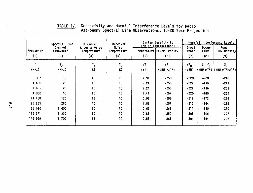
Frequency (1)

f (MHz)

327 1 420 1 665 4 830

14 488 ~ 22 235 . ~ 88 630

115 271 146 969

TABLE IV. Sensitivity and Hannfui Interference Levels for Radio Astronomy Spectral Line Observations, 10-20 Year Projection

Spectral Une Minimum Receiver System Sensitivity Harmful Interference Levels Channel Antenna Noise Noise (Noise Fluctuations) Input Power Power

Bandwidth Temperature Temperature Temperature Power Density Power Flux Flux Density (2) (3) (4) (5} (6) (7) {8} (9)

fc TA TR tiT tiP tiPH SH fc SH (kHz) ( K} ( K) (mK} (dBW Hz- 1 ) (dBW) (dBW m- 2 } (dBW m- 2Hz- 1 )

' 10 40 10 7. 91 -250 -220 ! -208 -248 20 10 10 2.24 -255 -222 -198 -241 20 10 10 2.24 -255 -222 -196 -239 50 10 10 1.41 -257 -220 -185 -232

170 15 10 0.96 -259 -216 -172 -224 250 40 10 1. 58 -257 -213 -164 -218

1 000 30 10 0.63 -261 -211 -150 -210 1 300 50 10 0.83 -259 -208 -146 -207 l 700 35 10 0.55 -261 -209 -144 -206

Rep. 223-4

SECTION 2E: RADIOASTRONOMY AND RADAR ASTRONOMY

Recommendations and Reports

REPORT 223-4

LINE f"REQUENCIES, ARISING FROM NATURAL PHENOMENA, OF INTEREST

TO RADIOASTRONOMY AND RELATED SCIENCES

(Question 5-1 /2)

365

(1963 - 1966 - 1970- 1974- 1978)

The amount of scientific information obtained from radioastronomical observations has greatly increased in recent years. Technology improvements in receivers and antennae have been partly responsible for this increase. Astronomical observations have now been made from ground based observatories using radio techniques, at wavelengths shorter than 1 mm (300 GHz), employing cooled bolometric detectors or various solid state devices. Thus from the point of view of availability of equipment, the entire radio spectrum can now be employed for astronomical measurements.

Another reason for the rapid growth of interest, particularly in that part of the spectrum from 100 MHz to 300 GHz, has been the discovery of line radiation from a number of extra-terrestrial substances of astrophysical importance.

First, there are many discrete spectral lines called "recombination lines" that arise when atoms of hydrogen, helium, carbon, etc. gain or lose energy as their electrons jump from one orbit to another under different conditions of atomic excitation. The first of these lines was discovered in space in 1964 by radio astronomers in the U.S.S.R. [Sorotchenko, et al., 1964). These lines are numerous and spread throughout the radio spectrum [Lilley and Palmer, 1968). Through careful observation of the strengths and shapes of these lines, radio astronomers are able to determine the physical conditions such as temperature, density and the extent of ordered or random motions of any celestial object in which recombination lines are found.

Second, there have been discoveries of emission or absorption lines arising in interstellar space due to neutral atomic hydrogen and' many inorganic and organic molecules. Following the first observation of the hyperfine spin-flip transition of hydrogen in 1951 [Ewen and Purcell, 1951), it was not until 1963 that the first molecular line (OH) was detected in the radio spectrum [Weinreb et al., 1963), and not until 1968 that other molecules were observed. However, since then many more interstellar molecules have been identified, the majority by means of spectral lines at millimetre wavelengths. Table I lists, in order of increasing frequency, the lines of interstellar organic and inorganic molecules reported by radio astronomers. The first column in each table gives the frequency; the second column lists. the molecular formula and name, and the third column indicates whether the spectral line has been observed in absorption (A) or emission (E). A double asterisk in this column indicates that the line is afforded at least footnote recognition by the World Administrative Radio Conference for Space Telecommunications, Geneva, 1971. It is realized that only some of these lines can be afforded protection in the Radio Regulations by allocations, and the astrophysically most important lines are listed in Report 224-4 and Recommendation 314-4.

The formation mechanism for interstellar molecules is not well understood. For typical interstellar cloud densities ranging between one and one million molecules per cubic centimetre and temperatures between 10 K and 100 K, the time between molecular collisions ranges from one thousand years to one third of a day. Thus typical conditions in interstellar clouds do not enhance collisional formation of polyatomic molecules although it is possible to explain the presence of CH, CH+ and CN by invoking radiative association. Also, recent laboratory determinations of lifetime against photo dissociation [Steif et al., 1972), indicate that, given an ambient ultraviolet radiation field of 4 x l0- 17 ergs cm- 3 A- 1 [Habing, 1968), it takes only ten years for unshielded interstellar carbonyl sulphide to be destroyed; thirty years for formaldehyde; forty years for ammonia; and one thousand years for carbon monoxide. Certainly, under these conditions an unshielded polyatomic molecule could not survive the harsh interstellar environment.

Even though molecular formation is not clearly understood, there are three reasons which appear to explain the remarkable observational results which radio astronomers are now obtaining. First, all the new molecules appear to be associated with regions of obscuration or interstellar dust. Experimentally, it has been found. that molecular lifetime with respect to photo dissociation increases tremendously with each increment of visual extinction. Thus once formed, a molecule may exist many orders of magnitude longer inside a dust cloud than it can in unshielded space before ultra-violet photo dissociation occurs. Second, radio waves are not significantly attenuated by dust particles which are of sub-micron size; hence, radio signals can penetrate clouds which completely attenuate optical waves. Third, the excitation requirements are low for radio detection of molecules. For example, optical astronomers require a background source of excitation of at least 15 000 K in order to observe optical absorption lines; thus a very sp!!cial geometry of a very hot star with an intervening

366 Rep. 223-4

molecular cloud of low opacity places stringent conditions on optical astronomy. On the other hand, thirty times less excitation energy will produce a typical molecular rotational transition. Thus radio detection does not require a bright, hot star with an intervening molecular cloud; the background source might be an ionized hydrogen region, infra-red star, radio galaxy, or even the 3 K isotropic background radiation.

As a direct consequence of the interstellar molecular radio spectroscopy of the past few years, a number of phenomena have been discovered which indicate that radio astronomers are studying a new area of chemistry. The detection of as yet unidentified molecules, such as X-ogen, emphasizes the role of a typical interstellar cloud as a unique chemical laboratory - a sample cell which would be difficult if not impossible, to duplicate in its entirety in terrestrial laboratories. With mean free paths as long as 1015 cm, low temperatures, and catalytic dust grain surfaces present, it is not unreasonable to expect future detection of interstellar molecules which cannot be observed terrestrially because of rapid collisional destruction or rapid recombination mechanisms. This new chemistry should not be considered exotic or unusual, however, as it is the common chemistry of the galaxy and man stands to gain a greater understanding of his galactic environment from it.

Long, painstaking observations which often require many hours of integration are needed by radio astronomers in order to achieve initial detection of most of these lines. Many more orders of magnitude of time and effort are expended in detecting each line in other gas clouds and to obtain the signal-to-noise ratios necessary to draw conclusions of astrophysical interest from the observations. In general, bandwidths of 0.2 per cent or more of the rest line frequency are required in order to observe all components of the Doppler-shifted observed line frequency of these clouds moving along the line-of-sight within our galactic system. Wider bandwidths will of course be required for extragalactic observations.

The choice of wavelength for astronomical observations naturally depends on the lines to be observed, but it may also be strongly influenced by the transmission properties of the Earth's atmosphere, i.e., by the location of the so-called "windows" in the atmosphere. The regions of interest for ground-based observations known at present, are shown schematically in Fig. I, based on Report 719 of Study Group 5. This Report contains the study of the attenuation in clouds at frequencies above 50 GHz. In general, the windows are defined by the resonances of molecular oxygen and water vapour. The abundance of other atmospheric constituents, for example, CO, NO, N02, etc., is sufficiently small that their presence in a window will not significantly alter the usefulness of this window for astronomical observations.

The curves in Fig. 1 show the total one-way absorption in the vertical direction for a dry atmosphere and for two representative atmospheres with water vapour concentrations of 0.5 and 7.5 g/m3 at the Earth's surface. These curves are based partly on theoretical calculations and partly on measurements. The model atmosphere adopted is one in which the water vapour concentration decreases exponentially with increasing height, the scale height being 2 km.

The Annexes summarize some of the types of spectral line observations that are being conducted at observatories throughout the world. The five Annexes deal with lines of atomic hydrogen and the four molecules OH, H20, H2CO and CO. These are not the only lines important to radioastronomy, and for historical reasons the selection doe~ not give full weight to the millimetre wave region of the spectrum. A more complete list is given in Recommendation 314-4. However, those included in the Annexes are a reasonably representative sample showing the kinds of observation made and the variety of results obtained. The Annexes also demonstrate how some of the significant conclusions concerning the nature of the Universe can be reached on the basis of spectral line observations.

REFERENCES

EWEN, H. I. and PURCELL, E. M. [1951) Nature, 168, 356. HADING, H.J. [1968) Bulletin Astr. Inst. Netherlands, 19, 421. LILLEY, A. E. and PALMER, P. [1968) Astrophys. lourn. (Suppl. Ser. 144), 16, 143. SOROTCHENKO, R. L., BORODZITCH, 0. S., DRAVSKIKH, Z. V. and KOLBASSOV, V. A. [1964) Proceedings of the Xllth

General Assembly of the International Astronomical Union, Hamburg. STEIF, L. J., DONN, B., GUCKER, S., GENTIEU, E. P. and MENTALL, J.E. [1972) Astrophys. Journ., 171, 21. WEINREB, S., BARRElT, A.H., MEEKS, M. L. and HENRY, J.C. [1963) Nature, 200, 829.

Rep. 223-4

TABLE I - Interstellar lines detected by radio asrronomers and the co"eiponding rest frequencies (from ref 1 o: Lovas et al., 19 78, unless otherwise ipecified in column 3) •

(up to August 1977)

367

Frequency (GHz) Molecule/ Atom Absorption (A) or emission (E)

(1) (2) (3)

0.834267 CH30H - methyl alcohol E

l.065075 CH3CH0 - acetaldehyde E

l.371709 CH2CHCN - vinyl cyanide E••

l.371794 CH2CHCN - vinyl cyanide E••

1.371947 CH2CHCN - vinyl cyanide EH

l.420406 H - hydrogen AandE••

1.538135 NH2CHO - form amide E

1.538693 NH2CHO - formamide. E

1.539295 NH2CHO - form amide E

1.539570 NH2CH0 - formamide E

1.539851 NH2CHO - formamide E

1.541018 NH2CHO - formamide E

1.610249 HCOOCH3 - methyl formate E

1.610906 HCOOCH3 - methyl formate E

l.6122310 OH - hydroxyl A andE**

l.62443 170H - hydroxyl Al

l.62617 17oH - hydroxyl Al

l.637564 18oH' - hydroxyl A

l.638805 HCOOH - formic acid E

l.639503 18oH - hydroxyl A

1.6654018 OH - hydroxyl A andE*•

1.6673590 OH - hydroxyl A and EH

1.7205300 OH - hydroxyl A and E••

2.66161 HCCCCCN - cyanodiacetylene E

2.66287 HCCCCCN - cyanodiacetylene E

2.66476 HCCCCCN - cyanodiacetylene E

3.139406 H2CS - thioformaldehyde A

3.195167 CH3CHO - acetaldehyde E

3.263794 CH - CH radical E

3.335481 CH - CH radical AandE

3.349193 CH - CH radical AandE

4.3887786 H2cl8o - formaldehyde A

4.3887960 H2c18o - formaldehyde A

4.3887963 H2c18o - formaldehyde A

4.3888011 H2C18o - formaldehyde A

4.3888035 H2cl8o - formaldehyde A

4.3888084 H2c 18o - formaldehyde A

4.5929563 H213co - formaldehyde A

4.5929738 H213co - formaldehyde A

4.5929759 H213co - formaldehyde A

4.5929857 H213co - formaldehyde A

4.5929934 H213co - formaldehyde A

4.5930494 H213co - fo~aldehyde A

• t•• Sec notes at the end of the Table.

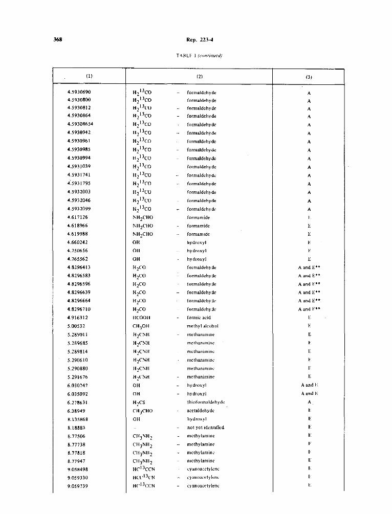
368 Rep. 223-4

Ti\llU I (co11ti11ued)

(I) (2) (3)

4.5930690 H2t3co - formaldehyde A 4.5930800 H213co - formaldehyde A 4.5930812 H213co -· formaldehyde A

4.5930864 H213co - formaldehyde A

4.59308654 H213co - formaldehyde A

4.5930942 H113co - formaldehyde A

4.5930961 H213co - formaldehyde A

4.5930985 Hit3co - formaldehyde A

4.5930994 H213co - formaldehyde A

4.5931039 H213co - formaldehyde A

4.5931741 H213co - formaldehyde A

4°.5931795 H213co - formaldehyde A

4.5932003 H213co formaldehyde A

4.5932046 Hil3co - formaldehyde A

4.5932099 Hzl3co - formaldehyd~ A

4.617126 NH 2CHO -· formamide !-.

4.618966 NH 2CHO - form amide L

4.619988 NH 2CHO - form amide E

4.660242 OH - hydroxyl E

4.750656 OH -·· hydroxyl E

4. 765562 OH hydroxyl E

4.8296413 H2co formaldehyde A and E ..

4.8296583 H2CO ·- formaldehyde A and E ..

4.8296596 HzCO - formaldehyde A and E**

4.8296639 H2CO - formaldehyde A and E**

4.8296664 H2co - formaldehyde A and E**

4.8296710 H2CO - formaldchy de A and E**

4.916312 HCOOH - formic acid E

5.00532 CH 30H methyl alrnhol E

5.289011 H2CNH - methanimine E

5.289685 H2CNH methaniminc E

5.289814 H2CNH mcthaniminc I·:

5.290610 H2CNH methaniminc E

5.290880 H2CNH - methaniminc F

5.291676 H2cNH - methanimine E

6.030747 OH - hydroxyl AandE

6.035092 OH - hydroxyl A and .E

6.278631 H1CS - thioforrnaldeh ydc A

6.38949 CH3CHO acetaldchyde E

8.135868 OH hydroxyl E

8.18883 - - not yet identified E

8.77506 CH3NH 2 - methylamine E

8.77738 CH 3NH 2 -· me thy lam inc E

8.77818 CH3NH 2 - mcthylaminc F

8.77947 CH3Nll 2 methylaminc E

9.058498 Hcl3ccN cyanoaeetylcne I·:

9.059330 Hcc13cN ·- cyanoaectylcnc F

9.059739 Hc13ccN - cyanoacctylenc F

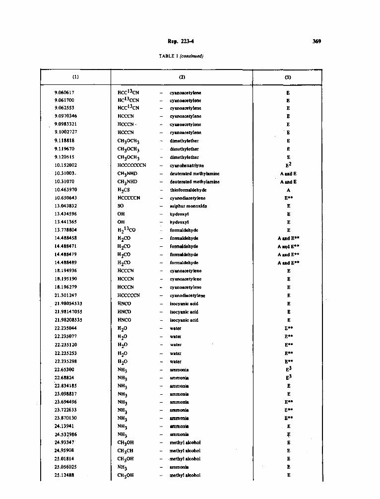
Rep. 2~ 369

TABLE I (continutd)

(1) (2) (3)

9.060617 nccl3cN - cyanoacetylene E 9.061700 ncl3ccN - cyanoacetylene E

9.062553 ncc13cN - cyanoacetylene E

9.0970346 HCCCN - cyanoacetylene E

9.0983321 HCCCN· - cyanoacetylene E

9.1002727 HCCCN - cyanoaoetylene E

9.118818 CH30CH3 - dimethylether E

9.119670 CH30CH3 - dimethylether E

9.120515 CH30CH3 - dimethylether E

10.152002 HCCCCCCCN - cyanohexatriyne £2

10.31003. CH3NHD - de11terated methylamine AIDdE

10.31070 CH3NHD - de11terated methylamine AIDdE

10.463970 H2CS - thloformaldehyde A

10.650643 HCCCCCN - cyanodiacetylene E ..

13.043832 so - S11lph11r monoxide E

13.434596 OH - hydroxyl E

13.441365 OH - hydroxyl E

13.778804 H213CO - formaldehyde E

14.488458 H2CO - formaldehyde AandE ..

14.488471 H2CO - formaldehyde A~4E ..

14.488479 H2CO - formaldehyde AID\IE ..

14.488489 H2CO - formaldehyde AIDdE••

18.194936 HCCCN - cyanoacetylene E

18.195190 HCCCN - cy1111oacetylene E

18.196279 HCCCN - cyanoacetylene E

21.301247 HCCCCCN - cyanodiacetylene E

21.98054533 HNCO - isocyanic acid E

21.98147055 HNCO - isocyanic acid E

21.98208535 HNCO - isocyanic acid E

22.235044 H2o - water E ..

22.235077 H20 - water E ..

22.235120 H2o - water E ..

22.235253 H20 - water EH

22.235298 H20 - water E ..

22.65300 NH3 - ammonia £3

22.68824 NH3 - ammonia El

22.834185 NH3 - ammonia E

23.098817 NH3 - ammonia E

23.694496 NH3 - ammonia £••

23.722633 NH3 - ammonia E ..

23.870130 NH3 - ammonia E ..

24.13941 NH3 - ammonia E

24.532986 NH3 - ammonia ~ 24.93347" CH30H - methyl alcohol E

24.95908 CH3CH - methyl alcohol E

25.01814 CH30H - . methyl alcohol E

25.056025 NH3 - ammonia E

25.12488 CH30H - methyl alc9hol E

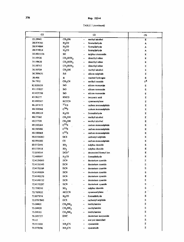
370 Rep. 2234

TABLE 1 (continued)

(1) (2) (3)

25.29441 CH30H - methyl alcohol E 28.974781 H2CO - formaldehyde A 28.974804 H2CO - formaldehyde A 28.974814 H2CO - formaldehyde A

30.0015236 so - sulphur monoxide E

31.10526 CH30CH 3 - dimethyl ether E

31.10620 CH3ocH3 - dimethyl ether E

31.10712 CH30cH3 - dimethyl ether E

36.16924 CH30H - methyl alcohol E

36.309631 SiS - silicon sulphide E

36.466 H - excited hydrogen E 36.7952 CH3CN - methyl cyanide E4

42.820539 SiO - silicon monoxide E

43.122027 SiO - silicon monoxide E

43.423798 SiO - silicon monoxide E

43.96277 HNCO - isocyanic acid E

45.490307 HCCCN - cyanoacetylene E

46.247472 13cs - carbon monosulphide E

48.206948 c34s - carbon monosulphide E

48.284519 H2CO - formaldehyde E

48.37260 CH30H - methyl alcohol E

48.37709 CH30H - methyl alcohol E

48.583264 c33s - carbon monosulphide E

48.585906 c33s - carbon monosulphlde E

48.589068 c33s - carbon monosulphide E

48.6516063 ocs - carbonyl sulphide E

48.991000 cs - carbon monosulphide E

68.972145 S02 - sulphur dioxide E

69.575918 S02 - sulphur dioxide E

72.039354 oco+ - deuterated formyl ion E

72.409097 H2CO - formaldehyde E

72.4134843 DCN - deuterium cyanide E

72.4135143 DCN - deuterium cyanide E

72.4135584 DCN - deuterium cyanide E

72.4149054 DCN - deuterium cyanide E

72.4149270 DCN - deuterium cyanide E

72.4149732 DCN - deuterium cyanide E

72.4170297 DCN - deuterium cyanide E

72.758210 SOz - sulphur dioxide E

72.783822 HCCCN - cyanoacetylene E

72.837974 Hz CO - formaldehyde E

72.9767845 ocs - carbonyl sulphide E

73.04401 CH3NH2 - methylamine E

73.04420 CH3NH2 - methylamine E

73.04515 CH3NH2 - methylamine E

76.305727 DNC - deuterium isocyanide E

79.15 - - not yet identified E

79.915101 NH2CN - cyanamide E

79.979596 NH2CN - cyanamide E

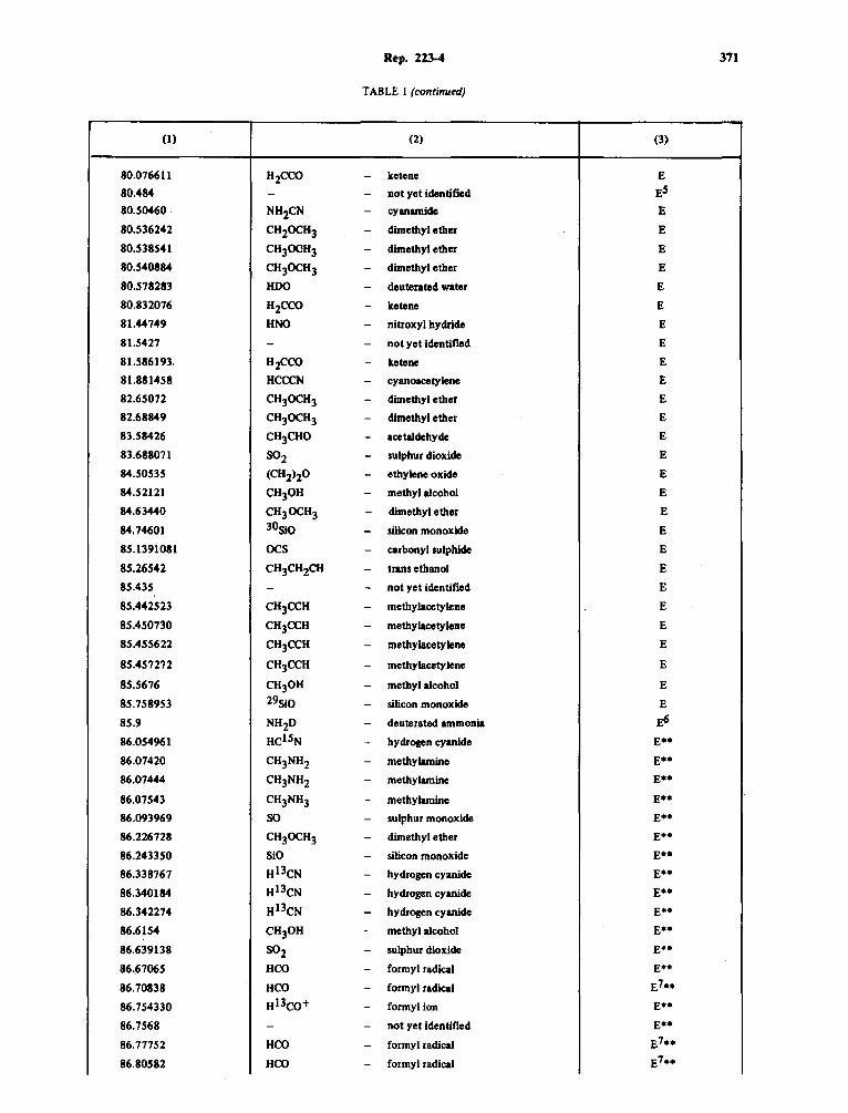
Rep. 223-4 371

TABLE 1 (continued)

(1) (2) (3)

80.076611 H2COO - ketene E

80.484 - - not yet identified ES

80.50460. NH2CN - cyanainide E

80.536242 CH20CH3 - dimethyl ether E

80.538541 CH300H3 - dimethyl ether E

80.540884 CH30CH3 - dimethyl ether E

80.578283 HOO - deuterated water E

80.832076 H2CCO - ketene E

81.44749 HNO - nitroxyl hydride E

81.5427 - - not yet identified E

81.586193. HzCOO - ketene E

81.881458 HCCCN - cyanoacetylene E

82.65072 CH30CH3 - dimethyl ether E

82.68849 CH30CH3 - dimethyl ether E

83.58426 CH3CHO - acetaldehyde E

83.688071 S02 - sulphur dioxide E

84.50535 (CH2>20 - ethylene oxide E

84.52121 CH30H - methyl alcohol E

84.63440 CH30CH3 - dimethyl ether E

84.74601 30Si0 - silicon monoxide E

85.1391081 ocs - cubonyl sulphide E

85.26542 CH3CH2CH - trans ethanol E

85.435 - - not yet identified E

85.442523 CH3CCH - methylacetylene E

85.450730 CH3CCH - methylacetylene E

85.455622 CH3CCH - methylacetylene E

85.457272 CH3CCH - methylacetylene E

85.5676 CH30H - methyl alcohol E

85.758953 29s10 - silicon monoxide E

85.9 NH2D - deuterated ammonia E6

86.054961 Hcl5N - hydrogen cyanide E••

86.07420 CH3NH2 - methylamine E••

86.07444 CH3NH2 - methylamine E••

86.07543 CH3NH3 - methylamine E••

86.093969 so - sulphur monoxide E ..

86.2267211 CH30CH3 - dimethyl ether E••

86.243350 SiO - silicon monoxide E••

86.338767 Hl3cN - hydrogen cyanide E ..

86.3401114 Hl3cN - hydrogen cyanide E ..

86.342274 Hl3cN - hydrogen cyanide E**

86.6154 CH30H - methyl alcohol E••

86.639138 S02 - sulphur dioxide E"*

86.67065 HOO - formyl radical E**

86.701138 HOO - formyl radical E7 ..

86.754330 H13oo+ - formylion E**

86.7568 - - not yet identified E**

86.77752 HOO - formyl radical E7 ..

86.80582 HCO - formyl radical E7••

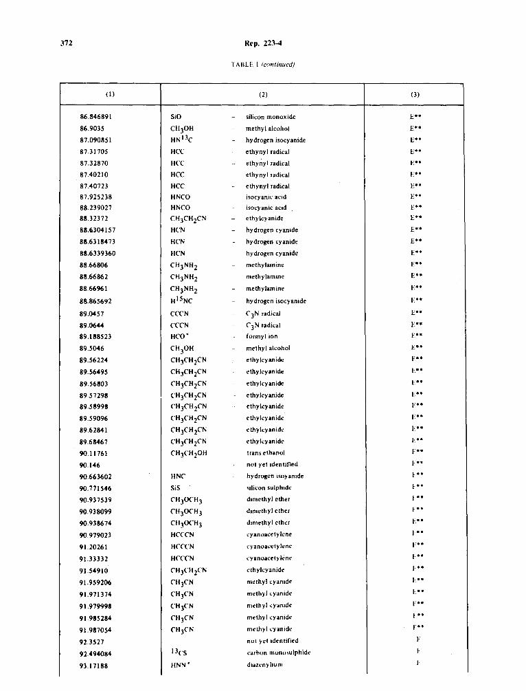
372 Rep. 223-4

TABLF I (continued)

(I) (2) (3)

86.846891 SiO - silicon monoxide E ..

86.9035 CH30H - methyl alcohol 1::•• 87.090851 HNl3c ·- hydrogen isocyanide E•• 87.31705 HCC ethynyl radical E ..

87.32870 HCC - ethynyl radical E ..

87.40210 HCC - ethynyl radical E**

87.40723 HCC - ethynyl radical E•• 87.925238 HNCO - isocyanic acid E ..

88.239027 HNCO - isocyanic acid E**

88.32372 CH3cH2CN - ethylcyanide E ..

88.6304157 HCN - hydrogen cyanide E ..

88.6318473 HCN - hydrogen cyanide E•• 88.6339360 HCN hydrogen cyanide E•• 88.66806 CH3NH 2 - methylaminc E••

88.66862 CH3NH 2 methylamine E•• 88.66961 CH3NH2 - methylamine E**

88.865692 H15 NC - hydrogen isocyanide F**

89.0457 CCCN - c 3N radical E•• 89.0644 CCCN - c3N radical i-:•• 89.188523 Hco+ - formyl ion E**

89.5046 cH 30H methyl alcohol E ..

89.56224 CH3CH 2CN ethylcyanidc E**

89.56495 CH3CH 2CN ethykyanide l·: ..

89.56803 CH3CH 2CN ethylcyanide E•• 89.57298 CH3CH2CN ethykyanide i-:•• 89.58998 CH 3CHzCN ethylcyanide E•• 89.59096 CH3CHzCN cthylcyanide t-:•• 89.62841 CH3CH 2CN cthykyan1dc I·.••

89.68467 CH3CHzCN ethykyanidc ...... 90.11761 CH3CH20H trans ethanol ..... 90.146 not yet identified I·••

90.663602 HNC hydrogen isuy amde I·••

90.771546 SiS 'llicon sulphide I·••

90.937539 CH30CH3 dimethyl ether I·••

90.938099 CH30CH3 dimethyl ether i:•• 90.938674 CH30CH3 dimethyl ether E ..

90.979023 HCCCN cyanoacety lcne I·••

91.20261 HCCCN cyanoa.:etylcne I·••

91.33332 HCCCN .:yanoat·etylene I·••

91.54910 CH3CHzCN cthykyanide I·••

91.959206 CH3CN methyl cyanide I·_••

91.971374 CH3CN methyl cyanide I·••

91.979998 CH3CN methyl cyanide i:••

91.9115284 CH3CN methyl cyanide I·••

91.9117054 CH3C'N methyl ,·yamde , ... 92.3527 not yet identified F

92.494084 Iles rarhon monmulphidt• I·

93.17188 HNN• diaun~lium I

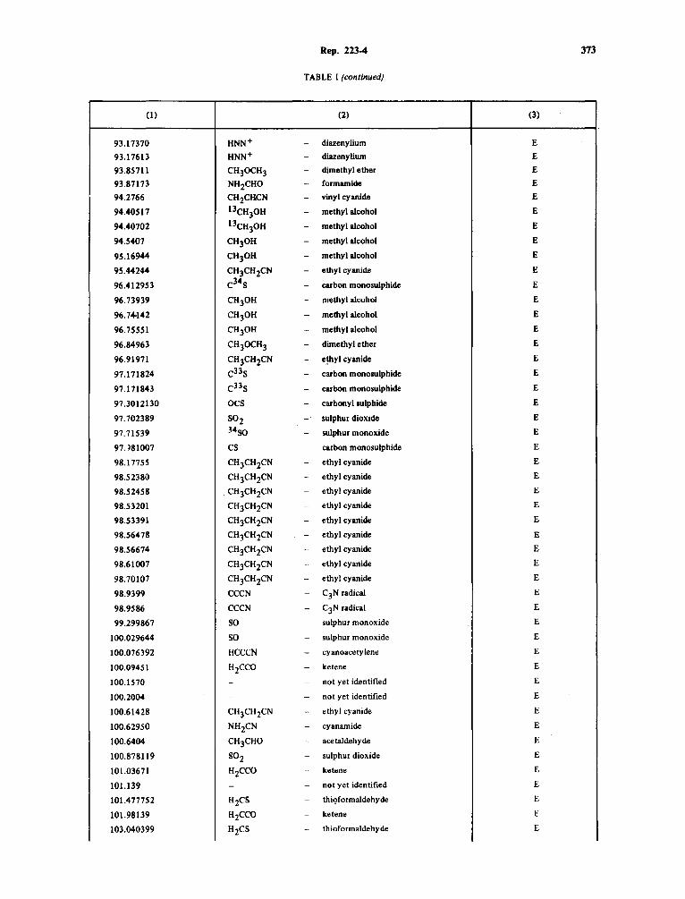
Rep. 223-4 373

TABLE I (continued)

(1) (2) (3)

93.17370 HNN+ - diazenylium E

93.17613 HNN+ - diazenylium E

93.85711 CH30CH3 - dimethyl ether E

93.87173 NH2CHO - formamide E

94.2766 CH2CllCN - vinyl cyanide E

94.40517 13cH30H - methyl alcohol E

94.40702 13cH30H - methyl alcohol E

94.5407 CH30H - methyl alcohol E

95.16944 cH30H - methyl alcohol E

95.44244 CH3CH2CN - ethyl cyanide E

96.412953 c34s - carbon monosulphide E

96.73939 CH30H - methyl alcohol E

96.74-142 CH30H - methyl alcohol E

96.75551 CH30H - methyl alcohol E

96.84963 CH30CH3 - dimethyl ether E

96.91971 CH3CH2CN - e~yl cyanide E

97.171824 c33s - carbon monosulphide E

97.171843 c33s - carbon monosulphide E

97.3012130 ocs - carbonyl sulphide E

97.702389 S02 - sulphur dioxide E

97.71539 3450 - sulphur monoxide E

97. ~81007 cs - carbon monosulphide E

98.17755 CH3CH2CN - ethyl cyanide E

98.52380 CH3CH2CN - ethyl cyanide E

98.52458 CH3CH2CN - ethyl cyanide E

98.53201 CH3CH2CN - ethyl cyanide E

98.53391 CH3CH2CN - ethyl cyanide E

98.56478 CH3CH2CN - ethyl cyanide E

98.56674 CH3CH2CN - ethyl cyanide E

98.61007 CH3CH 2CN - ethyl cyanide E

98.70107 CH3CH2CN - ethyl cyanide E

98.9399 CCCN - c 3N radical E

98.9586 CCCN - c 3N radical E

99.299867 so - sulphur monoxide E

100.029644 so - sulphur monoxide E

100.076392 HCCCN - cyanoacetylene E

100.09451 HzCCO - ketene E

100.1570 - - not yet identified E

100.2004 - - not yet identified E

100.61428 CH3CH2CN - ethyl cyanide E

100.62950 NH2CN - cyanamide E

100.6404 CH3CHO - acetaldehyde E

100.878119 SOz - sulphur dioxide E

101.03671 HzCCO - ketene E

101.139 - - not yet identified E

101.477752 H2CS - thi9formaldehyde E

101.98139 H2CCO - ketene E

103.040399 HzCS - thioformaldehyde E

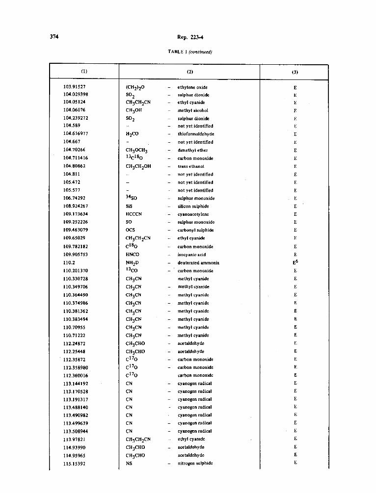
374 Rep. 223-4

TABLE I (continued)

(1) (2) (3)

103.91527 (CH2)20 - ethylene oxide E

104.029398 so2 - sulphur dioxide E 104.05124 CH3CH2CN - ethyl cyanide E

104.06076 CH30H - methyl alcohol E

104.239272 S02 - sulphur dioxide E 104.589 - - not yet identified E

104.616977 H2CO - thioformaldehyde E

104.667 - - not yet identified E

104.70266 CH30CH3 - dimethyl ether E

104.711416 nc180 - carbon monoxide E

104.80862 CH3CH20H - trans ethanol E

104.811 - - not yet identified E

105.472 - - not yet identified E

105.577 - - not yet identified E

106.74292 34so - sulphur monoxide E

108.924267 SiS - silicon sulphide E

109.173634 HCCCN - cyanoacetylene E

109.252226 so - sulphur monoxide E

109.463079 ocs - carbonyl sulphide E

109.65029 CH3CH2CN -· ethyl cyanide E

109.782182 cl8o - carbon monoxide E

109.905753 HNCO - isocyanic acid E

110.2 NH2D - deuterated ammonia E6

110.201370 13co - carbon monoxide E

110.330728 CH3CN - methyl cyanide E

110.349706 CH3CN - methyl cyanide E

110.364490 CH3CN - methyl cyanide E

110.374986 CH3CN - methy I cyanide E

110.381362 CH3CN - methyl cyanide E

110.383494 CH3CN - methyl cyanide E

110.70955 CH3CN - methyl cyanide E

110.71222 CH3CN - methyl cyanide E

112.24872 CH3CHO - acetaldehyde E

112.25448 CH3CHO - acetaldehyde E

112.35872 c17o - carbon monoxide E

112.358980 cl7o - carbon monoxide E

112.360016 c17o - carbon monoxide E

113.144192 CN - cyanogen radical E

113.170528 CN - cyanogen radical E

JI 3.191317 CN - cyanogen radical E

113.488140 CN - cyanogen radical E

113.490982 CN - cyanogen radical E

113.499639 CN - cyanogen radical E

113.508944 CN - cyanogen radical E

113.97821 CH3CH2CN - ethyl cyanide E

114.93990 CH3CHO - acetaldehyde E

114.95965 CH3CHO - acetaldehyde E

115.15392 NS - nitrogen sulphide E

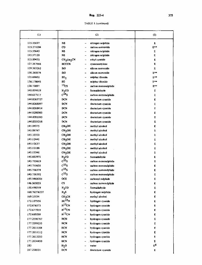
Rep. 223-4 375

TABLE I (continued}

(1) (2) (3)

115.15697 NS - nitrogen sulphide E

115.271204 co - carbon monoxide E ..

115.55643 NS - nitrogen sulphide E

115.57120 NS - nitrogen sulphide E

115.89435 CH3CH2CN - ethyl cyanide E

127.367666 HCCCN - cyanoacetylene E

129.363262 SiO - silicon monoxide E

130.268574 SiO - silicon monoxide E**

135.69602 S02 - sulphur dioxide E**

138.178645 so - sulphur dioxide E**

138.73897 13cs - carbon monosulphide Eu

140.839529 H2co - formaldehyde E

144.617117 c34s - carbon monosulphide E

144.8265727 DCN - deuterium cyanide E

144.8268097 DCN - deuterium cyanide E

144.8268414 DCN - deuterium cyanide E

144.8280003 DCN - deuterium cyanide E

144.8281093 DCN - deuterium cyanide E

144.8303358 DCN - deuterium cyanide E

145.09375 CH30H - methyl alcohol E

145.09747 CH30H - methyl alcohol E

145.10323 CH30H - methyl alcohol E

145.12441 CH30H - methyl alcohol E

145.12637 CH30H - methyl alcohol E

145.13188 CH30H - methyl alcohol E

145.13346 CH30H - methyl alcohol E

145.602971 H2CO - formaldehyde E

145.755619 c33s - carbon monosulphide E

145. 755635 c33s - carbon monosulphide E

145.756374 c33s - carbon monosulphide E

145.756392 c33s - carbon monosulphide E

145.9468205 ocs - carbonyl sulphide E

146.969039 cs - carbon monosulphide E

150.498359 H2CO - formaldehyde E

168. 76276237 H2S - hydrogen sulphide E

169.33534 CH3CH - methyl alcohol E

172.107956 He I SN - hydrogen cyanide E

172.676573 Hl3CN - hydrogen cyanide E

172.677959 Hl3CN - hydrogen cyanide E

172.680209 H13cN - hydrogen cyanide E

177.2596767 HCN - hydrogen cyanide E

177.2599233 HCN - hydrogen cyanide E

177.2611104 HCN - hydrogen cyanide E

177.2611112 HCN - hydrogen cyanide E

177.2612232 HCN - hydrogen cyanide E

177.2634450 HCN - . hydrogen cyanide E

183 H20 - water ES

217.238531 DCN - deuterium cyanide E

376 Rep. 223-4

TAFILF I (continued)

(1) (2) (3)

219.560369 cIBo - carbon monoxide E

220.398714 13co - carbon monoxide E

230.538001 co - carbon monoxide E ..

345 co - carbon monoxide E9

* A complete list of radio atomic and molecular lines is given in order to facilitate protection arrangements. There are also a large number of important recombination lines of hydrogen, helium, carbon etc. A full table of recombination line frequencies is available !Lilley and Palmer (1968)).

** Afforded some measure of protection by the Radio Regulations.

REFERENCES (TABLE I)

I. GARDNER, F. F. and WHITEOAK, J.B. [1976). Monthly Notes of the Royal Astronomical Society, 176, 57. 2. KROTO, H. W., KIRBY, C., WALTON, D.R. M., AVERY, L. W., BRUTEN, N. W., OKA, T. and MACLEOD, J.M.

[1977). Bulletin of the American Astronomical Society, 9, 303. 3. SWEITZER, J. S., PALMER, P., MORRIS, M., TURNER, B. E. and ZUCKERMAN, B. [1977) 811/Jetin of the

American Astronomical Society, 9, 373. 4. BLACKMAN, G. L., BROWN, R. D., GODFREY, P. D., BASSEZ, M. P .. OTIREY, A. L., WRJNKLER, D. and

ROBINSON, B. J. [1977). Monthly Notes of the Royal Astronomical Society, 180, I.

5. TURNER, B. E., KISLYAKOV, A.G., LISZT, H. S. and KAirU, N., (1975] Astrophys. Journ. (Letters), 201, L 149. 6. BLAKE, B. H. and PALMER, P. [1977) Bulletin of the American Astronomical Society, 9, 429. 7. SNYDER, L. E., HOLLIS, J.M. and ULICH, B. L. [1976] Astrophys. Journ. (Letters), 208, L 91. 8. WATERS, J. W., GUSTINCIC, J. J., KAKAR, R. K., KUIPER, T. B. H., SWANSON, P. N., KERR, A. R. and

THADDEUS, P. [ 1976) Bu/Jetin of the American Astronomical Society, 8, 564. 9. HUGGINS, P. J., PHILLIPS, T. G., NEUGEBAUER, G., WERNER, M. V., WAN NIER, P. G. and ENNIS, D. [1977)

Bulletin of the American Astronomical Society, 9, 353. IO. LOVAS, F. J., JOHNSON, D.R. and SNYDER. L. E. [1978], Astrophys. Journ. Suppl. (in preparation).

ANNEX I

THE NEUTRAL HYDROGEN UNI:. AT 1420.406 MHz

Emission from atomic hydrogen occurs from a hyperfine spin-nip transition at the ground level of the atom. This emission was first observed in 1951 [Ewen and Purcell, 1951 ]. The study of the neutral hydrogen component of the interstellar medium is particularly suitable for a number of fundamental astronomical problems. Hydrogen, the most abundant element in the Universe, is also the main observed constituent of the interstellar medium. The motions and distribution of hydrogen are closely related to those of other galactic constituents, both stellar and interstellar. The interstellar medium is transparent enough to radio emission at 1420 MHz, so that, with the exception of a few directions along the galactic equator, it is possible to investigate the entire Milky Way galaxy and other distant galaxies. This transparency allows investigation of regions of the Milky Way which are too distant, or are too obscured by dust in the interstellar medium, to be studied optically. Interstellar neutral hydrogen is so abundant and is distributed in such a general fashion throughout the galaxy, that the emission line has been detected at every direction in the sky at which a suitably equipped radio telescope has been pointed. No time variation of this line has been found. Many 21-cm surveys of galactic hydrogen have been published. These are listed by [Kerr, 1969) and [Burton, 1974] and [Heiles and Wrixon, 1976].

What is detected is a line profile giving intensity, usually expressed as a brightness temperature, as a function of frequency. The frequency observed for the line may indicate a Doppler shift from the natural rest frequency of 1420.406 MHz. The Doppler-shift information inherent in observations of hydrogen within .a galaxy is very important since it allows the kinematic distribution of the gas to be studied, in addition to the spatial distribution of intensities. In practice, the measured frequency shifts are converted to radial velocities. At 1420 MHz, a velocity of recession of I km/s corresponds to a reduction in frequency of 4.74 kHz. The natural width of the neutral hydrogen line is 5 x JO- 1" Hz and is thus infinitesimally s111all <:om pared to that which can be measured by radioastronomical methods. However, profiles observed near the Milky Way typically extend over 500 kHz. This broadening occurs throughout several mechanisms. The broadening corresponding to the thermal velocities of atoms within a single concentration of gas is typically 5 or 10 kHz. Turbulent motions within a concentration of hydrogen gas will also produce profile broadening of this order of magnitude. Large-scale streaming motions with Doppler-shift amplitudes of the order of 30 kHz have been observed in our galaxy and in others, and these motions influence the measured width of features in a profile. However, most of the total line broadening in galaxies comes from the differential rotation of the galaxy as a whole. For many galaxies this rotation broadens the profiles by 2500 kHz. Large-scale expansion motions in the still poorly understood central region of the Milky Way result in profiles broadened by a similar amount.

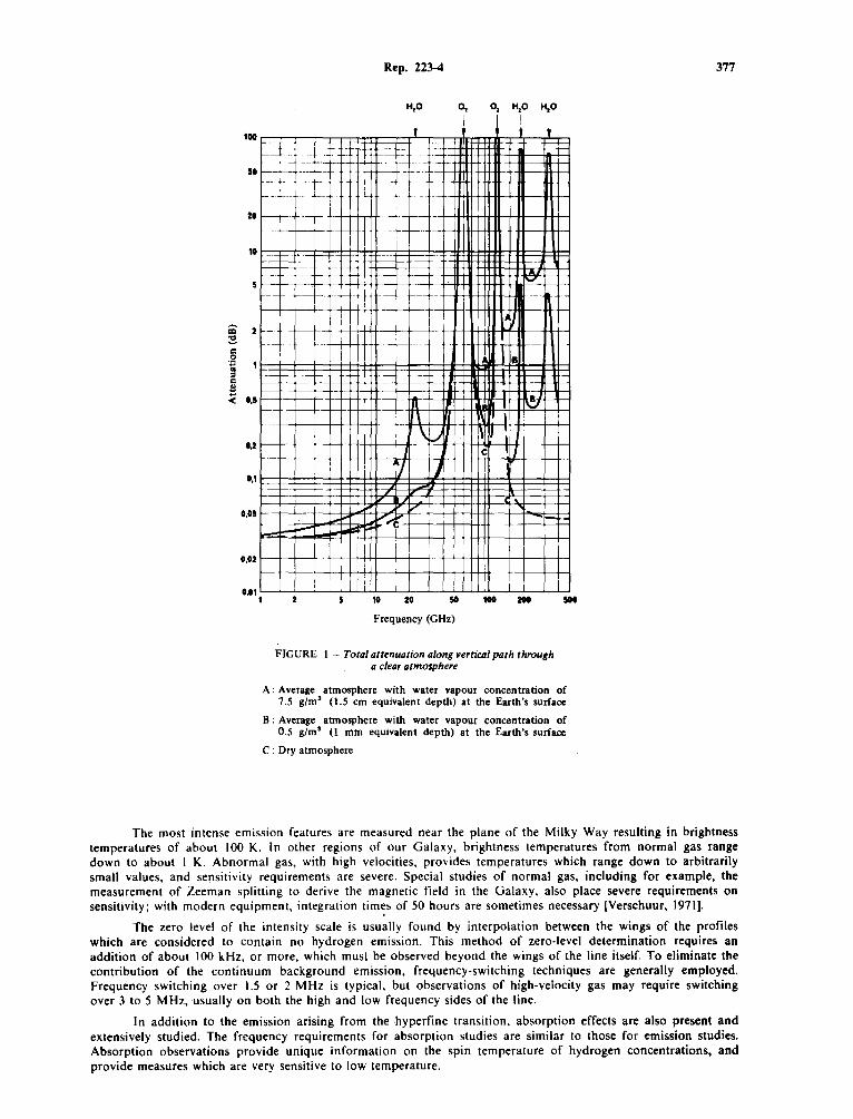
= ~ c: .g .. " c: $

<

Rep. 223-4

H20 o, 0, H,O H20

100 i ' ~ - <-- -- --~

50 >---- 1---- 1----- - - - ·- ~- - ~

21 ~ ~ + -- ··-~--·· ~-~

10 1--· 1---1---- - I-- ~-

~ 1---- --· I--

5 -~-

Ii 2

I. I

•.s ~ L--

" I

\ 1 \u '

0,2 I

I c I

0,1 '/ ~

, . 0,05 _ ....

,,,.-~"" / - -

'----- -=

0,02 -t-i I

I : i

•.•1, I I

10 20 50 100 2" sot

Frequency (GHz)

FIGURE I - Total attenuation along vertical path through a clear atmosphere

A: Average atmosphere with water vapour concentration of 7 .5 g/m 3 (1.5 cm equivalent depth) at the Earth's surface

B : Average atmosphere with water vapour concentration of 0.5 g/m" (1 mm equivalent depth) at the Earth's surface

C : Dry atmosphere

377

The most intense em1ss1on features are measured near the plane of the Milky Way resulting in brightness temperatures of about 100 K. In other regions of our Galaxy, brightness temperatures from normal gas range down to about I K. Abnormal gas, with high velocities, provides temperatures which range down to arbitrarily small values, and sensitivity requirements are severe. Special studies of normal gas, including for example, the measurement of Zeeman splitting to derive the magnetic field in the Galaxy, also place severe requirements on sensitivity; with modern equipment, integration timc;s of SO hours are sometimes necessary [Verschuur, 1971].

The zero level of the intensity scale is usually found by interpolation between the wings of the profiles which are considered to contain no hydrogen emission. This method of zero-level determination requires an addition of about 100 kHz, or more, which must be observed beyond the wings of the line itself. To eliminate the contribution of the continuum background emission, frequency-switching techniques are generally employed. Frequency switching over 1.5 or 2 MHz is typical, but observations of high-velocity gas may require switching over 3 to S MHz, usually on both the high and low frequency sides of the line.

In addition to the emission arising from the -hyperfine transition, absorption effects are also present and extensively studied. The frequency requirements for absorption studies are similar to those for emission studies. Absorption observations provide unique information on the spin temperature of hydrogen concentrations, and provide measures which are very sensitive to low temperature.

378 Rep. 223-4

External galaxies exhibit the well-known "red shift", a decrease of the observed frequency dependent on the distance of the galaxy. Receivers used at present allow successful studies to be made at intensities below 0.0 I jansky •. Most normal spiral galaxies at this nux density level have radial velocities of 4000 to 6000 km/s, and therefore are observed at frequencies down to 1390 MHz. The number of normal galaxies for which hydrogen-line data are available is approximately 500; this number is increasing rapidly, and is being augmented by investigations of nearby dwarf galaxies which were heretofore undetectable. These studies are important for determining the gross properties of galaxies such as distance, mass and hydrogen content. Data on a wide variety of objects will facilitate the development of theories of galactic formation and evolution. Concurrently, detailed synthetic aperture observations of the larger nearby galaxies are being made to confirm theories of spiral structure.

Some of the most exciting and important present day radio observations involve detection of the observed hydrogen· line in distant continuum sources. These have been accomplished for the radio galaxy Perseus A [De Young et al., 1973) and for the quasi-stellar objects 3C 286 [Brown and Roberts, 1973) and AO 0235 + 164 [Roberts et al., 1976). The detection of red-shifted 21 cm radiation from AO 0235 + 164 is of great cosmological significance. Since red-shifted optical lines (Mg+) had been previously detected in this source it became possible to make a direct comparison between the radio and optical red-shifts over a large cosmological distance. The fact that the radio and optical red-shifts agreed to within the experimental uncertainties ( 1 parl in 5000 for the optical measurement, and I part in 50 000 for the radio), allows one to place upper limits on the time variations of the physical constants which enter the atomic theory of spectroscopy.

H,istorically, the first line to be detected in the radio spectrum, the 21-cm hydrogen line, continues to grow in importance. The development of sensitive receivers has broadened the scope of extra-galactic studies to include objects with large Doppler shifts. Current observational programmes are directed towards obtaining spectra of large numbers of galaxies having emission frequencies at and below 1370 MHz at intensities of about 0.01 jansky. At the same time, detailed studies of our own and nearby galaxies are continuing between 1415 and 1427 MHz.

REf'F.RENCES

BROWN, R. L. and ROBERTS, M. S. [1973) A.-crophys. Journ., 184, L7.

BURTON, W. B. (1974) Galactic and extragalactic radio a.,tronomy. Eds. G. L. Verschuur and K.L. Kellermann, Springer-Verlag, 82.

DE YOUNG, D.S., ROBERTS, M. ~·and SASLAW, W. C. (1973) Astrophys. Journ., 185, 809.

EWEN, H. I. and PURCELL, E. M. [1951) Nature, 168, 356.

HEILES, C. and WRIXON, G. [1976), Method-' ofexperimenliil physics, UC, ed. M. L. Meeks (Academic Press: New York), 58.

KERR, F. J. [1969) Annual Review of Ascron. Astrophys., 7 39.

ROBERTS, M. S., BROWN, R. L., BRUNDAGE. W. D., ROTS, A.H., HAYNES. M. P. and WOLFE, A. M. [1976) Ascron. Journ., 81, 293.

VERSCHUUR, G. L. [1971) Astrophys. Journ., 165, 651.

ANNEX II

THE OH LINES IN RADIOASTRONOMY

1. Introduction

Radio-frequency spectral lines due to the hydroxyl molecule (OH) were first detected and measured in the laboratory in 1959 [Ehrenstein et al., 1959), and in interstellar space in 1963 [Weinreb et al., 1963). Absorption of radio-frequency radiation from the radio source Cassiopeia A was observed at frequencies** which correspond to those of the two principal ground state lines, at 1665.401 and 1667.358 MHz. Shortly afterwards, even stronger absorption lines were found from the region of the galactic centre [Bolton et al., 1964a; Robinson et al., 1964; Goldstein et al., 1964), and two expected subsidiary ground-state lines, arising from alternative configurations of spins within the OH molecule, were detected and their rest frequencies determined at 1612.231 and 1720.527 MHz [Goss, 1968). The very much lower intensity absorption line at 1639 MHz has been detected in the direction of the galactic centre [Rogers and Barrett, 1966). This line is due to the 0 18H molecule where the oxygen is the mass-18 isotope of the normal 0 16• Investigation of narrow-band emissions from regions of ionized hydrogen in the galaxy (Weaver et al., 1965; Zuckerman et al., 1965) identified them as arising from OH. This emission is unexpectedly intense, producing increases in antenna temperature of as much as 150 K, and it has, surprisingly, been found to have a circularly polarized component (Davies et al., 1966). A number of the sources of OH emission have now been studied with interferometers, to get more precise positions of the sources [Rogers et al., 1967) and estimates of the angular sizes of the sources [Davies et al., 1967). The new technique of "very long base-line" or VLB interferometry, with base-lines of length comparable with the diameter of the Earth, have been used to study some OH sources [Moran et al., 1967) and, also apparent angular sizes of less than 0.005 seconds of arc have been measured. This last technique, by an equipment improvement which is within the state of our present knowledge,

One jansky (Jy) = I flux unit (f.u.) = 10-2• W/m2

per Hz.

•• The frequencies in thi~ Report are the rest frequencies for the radiation concerned.

Rep. 223-4 379

opens up possibilities of using radio sources of very small angular size as position references for the location of the observing points on the Earth. Possible uses in measuring earth tides, continental drift, and accurate terrestrial rates of rotation, have been predicted (Gold, 1967; MacDonald, 1967].

The discovery of lines due to OH is of great astrophysical significance. The extent by which the observed frequencies are displaced from their rest frequencies by Doppler effects provides direct information about the motions of the gas clouds in which the OH occurs. The anomalies in the line intensities, both in emission and absorption, throw new and unexpected light on the physical conditions in particular regions of our galaxy. The observations also give more information on the structure of our galaxy.

2. The distribution or OH in the galaxy

Early survey work (Goss, 1968] showed, and later more thorough work (Turner, 1970; Turner, 1972) confirmed, that OH is very widely distributed throughout the galactic disk in a region within a few hundred parsecs • of the galactic plane. It is somewhat more closely confined to the plane than atomic hydrogen, and appears to be an excellent tracer of spiral arms. It does not appear to be closely associated with continuum sources, but rather to delineate the presence of dense neutral clouds of gas in a manner which is not possible optically or by means of 21-cm line of atomic hydrogen. This latter aspect has been of immense importance in the burgeoning studies of many other newly discovered interstellar molecules, as these molecules have been found in just these same dense clouds. In a literal sense, OH has proved to be the tracer molecule in the new field of interstellar molecular chemistry. Apart from its location in dense neutral gas clouds, OH has been discovered in some types of infra-red stars. A variety of other types of astronomical objects, such as planetary nebulae, Wolf-Rayet and T-Tauri stars, young and highly reddened stellar associations and clusters, do not yield observable OH to very low limits. It is anticipated that studies of physical conditions in these objects will shed light on the questions of formation and destruction of interstellar molecules in general, and OH in particular. Detection of OH in both absorption and emission has been made in comets, and research in this area is having important implications as to the origin and history of the solar system.

3. The properties or the absorption lines

The anomalies in the intensities of the lines when observed in absorption, continue to pose important problems, as these relative intensities in the observed lines sometimes differ considerably from the expected values for a source in thermodynamic equilibrium. For example, the absorption spectrum of the supernova remnant, Cassiopeia A, was examined at the frequencies of the two satellite lines, 1612 and 1720 MHz. Whereas both the 1665 and 1667 MHz transitions show splitting into two lines, neither the 1612 nor the 1720 MHz transition shows any splitting. Furthermore, the absorption at 1612 MHz is approximately one half of that at 1665 MHz, instead of one fifth, as expected. Finally, the observations indicate a small amount of OH emission at 1720 MHz, but none is detectable at 1612 MHz. The unusual absorption features and the presence of weak emission have been independently confirmed. It is very difficult to see how any of these observations can be explained in terms of a medium in thermodynamic equilibrium, and these observations are among the many that require further explanation. ·

Other absorption anomalies have been found in the•spectrum of the galactic centre (Robinson et al., 1964; Goldstein et al., 1964; Goss, 1968; Bolton et al., 1964b]. For example, the observed ratios of line intensities among the four lines are quite different from the ratios that are expected on the basis of thermal equilibrium. It is tempting to try to explain the observed values in terms of a medium exhibiting large attenuation, for which all ratios would approach unity, but this attempt fails. For example, isolated regions near the galactic centre show stronger absorption at 1665 than at 1667 MHz, and many regions show unequal absorption at 1612 and at 1720 MHz. It seems clear that these observations require the assumption of non-thermal distribution of the OH molecules among the internal energy states from which the radio lines are derived.

The OH observations in the galactic centre pose problems other than anomalous line-intensity ratios. OH absorption is very strong and extends over a considerable frequency, or velocity range. If OH profiles for the galactic centre are interpreted in a manner similar to that described for Cassiopeia A, then one derives on OH/H abundance ratio of - 10-4 some 103 times the ratio in the direction of Cassiopeia A. However, this value must be used with extreme caution, because any derived values, based upon observations, must await a full understanding of the mechanism by which OH is formed, how it is distributed with respect to its internal energy levels, and how it absorbs and emits radio energy. From the frequency at which OH absorption occurs, one can determine the velocity in the line-of-sight of the OH cloud relative to the Sun; and it is found that much of the OH is moving toward the galactic centre with a velocity of 40 km/s. This cloud also contains· other molecules and neutral hydrogen. On the other hand, most of the other gases associated with the galactic centre appear to be streaming away from the centre. The motions in the central region are clearly very complex. This is a curious situation and may force a revision of our ideas about the physical conditions in the galactic nucleus. It should be emphasized, though, that the observations tell us nothing about the distances to the OH and H; the concept that they are associated with the galactic centre rests strictly on interpretations of the accumulated evidence.

I parsec - 3.26 light years.

380 Rep. 223-4

4. The properties of the emission lines

The observations of the OH emission lines have similarly opened up a new and complex area of astronomical research. Early attempts to detect OH emission were confined to observations at 1667 MHz because it was thought this would be the strongest transition, but all attempts gave negative results. When OH was finally discovered in emission at 1665 MHz, not 1667 MHz, its properties were so unusual that two out of the first three groups of radio astronomers to observe it did not attribute the line to OH.

Australian observers first observed OH emission in June, 1964, when a narrow, intense emission line was detected to the side of an absorption line at 1665 MHz in the direction of the galactic centre (McGee et al., 1%5). However, the effect was apparently thought to be an instrumental effect and was not reported at the time. Six months or more later, OH emission was observed by groups at Harvard and Berkeley, with properties so unexpected that the Berkeley radio astronomers thought they had detected an unidentified micro-wave spectral line; they nicknamed the line "mysterium" until identification could be established. Although "mysterium" was almost immediately identified as OH, the name can hardly be called a misnomer in view of the strange properties exhibited in interstellar OH.

The first OH emission sources found, were characterized by intense, narrow emission lines at 1665 MHz, with lines of lesser intensity at the other three OH frequencies. Departures by several orders of magnitude from the expected intensity ratios were the rule; furthermore, the spectrum obtained at one frequency was usually completely uncorrelated with that obtained at another. This early type of OH emission source is now recognized as o~ly one of three distinctly different types of such sources. A second type radiates solely in the 1720 MHz line, while the third type has strongest emission at 1612 MHz but may be accompanied by weaker emission at both 1665 and 1667 MHz. While the peculiarities of these three types of emission source may appear random, in fact this is not so. Observationally, each type is rather well defined with respect to the relative intensities among the four lines, and each type also shows distinct polarization properties. Theoretically, models have been developed which, although probably not unique, do appear to explain the salient properties of each type of source.

The objects with which the various types of OH emission source are associated, are a major factor in the models proposed to explain them. Unlike the 21-cm emission of atomic hydrogen which is widely distributed throughout the Milky Way, each type of OH emission source is found only in special regions. The type associated with strong 1665 MHz emission is found only in isolated positions near ionized hydrogen regions, at positions where strong sources of infra-red are often found; while the type associated with strong 1612 MHz lines comes from the atmospheres of cool stars. The sources emitting in only the 1720 MHz line have a more obscure origin, although they are definitely not associated with stellar-like objects.

Between 1968 and 1971, a total of five different emission lines have been discovered which arise from transitions within excited rotational energy states of OH [Zuckerman et al., 1968; Yen et al., 1969; Turner et al., 1970]. Many other lines from these states which theoretically ought to be present are not found. This situation offers evidence as strong as that provided by the peculiar properties of the 18-cm lines, that the excitation of OH is in general not consistent with a medium in thermodynamic equilibrium. Observations of excited-state lines have also proved very valuable in distinguishing between the various theoretical models for anomalous excitation of OH.

~. The 0 18H and 0 17H lines

The strong OH absorption found in the direction of the galactic centre has made another experiment feasible. All the results discussed above have referred to the abundant isotopic species 0 16H, but the observation of strong absorption suggested the possibility that the isotopic species 0 18H and possibly also 0 17 H could be detected. The frequencies of these isotopes are shifted relative to those of the 0 16H lines because of mass­dependent effects on the molecular energy levels.

Early searches for the 0 18 H lines were successful [Rogers and Barrett, 1966; Wilson and Barrett, 1970]. Although weak as expected, both main lines (at 1637 and 1639 MHz) were detected in the galactic centre, and yielded an abundance ratio Q18H/0 16H of l/390, which is consistent with the terrestrial ratio for 0 18/0 16 of 11490 within the uncertainties in the observations.

Laboratory measurements of the 18 cm lines in the ground states of 0 18H and 0 17H have been made [Ball et al., 1970). Because of the nuclear spin of the 0 17 nucleus, there are many more hyperfine transitions within the ground state of 0 17 H than in the other two isotopes. However, the line strengths of only two of these 017H lines are strong enough to warrant astronomical searches with present equipment. These two lines, at 1624.4 and 1626.2 MHz have been found in the direction towards the galactic centre.

6. Positions and sizes of OH emission sources

The positions of a number of the OH sources have been determined to an accuracy of better than one second of arc [Rogers ct al., 1967]. The results have shown that an emission source can be a number of very small bright regions separated by angular distances of a few seconds of arc. The angular sizes of the regions themselves have been studied with interferometers of ever increasing base lines and angular resolutions. First results come with spacings between the antennae of 127 km, or 7 x 105 wavelengths [Davies et al., 1967], and these showed that one emitting region was less than 0.05 seconds of arc in size.

Rep. 223-4 381

The technique of very long base-line (VLB) interferometry began at about this time. In these experiments, two very distant radio telescopes observe the same source, and work as an interferometer because the local oscillator or phase reference at each telescope is derived from a highly stable rubidium maser. The resulting records for each telescope are subsequently carried to a computer and cross-correlated to develop the interference fringes. This technique was shown to work first for continuum observations [Broten et al., 1967; Bare et al., 1967]; but it is now extensively applied to OH line studies. As examples of base lines used, the radio telescopes at Hat Creek (University of California), Lincoln Laboratory (Massachusetts Institute of Technology, near Boston), National Radio Astronomy Observatory (Green Bank, West Virginia) and Onsala (near Gothenburg, Sweden) have all experimented on OH line work in pairs. The results show that OH emission sources can be as small as 0.005 seconds of arc in size. This li]nit may be still further reduced as experiments continue .

• If the frequency and phase stability of the VLB experiments can be improved (by the use of hydrogen

masers, for example), the technique may be usable for measuring the absolute positions of sources in the sky to better than 10- 3 seconds of arc. This in turn corresponds to position measures on Earth of 3 cm and the possibility of using such measures for a variety of geodetic and geophysical measurements is very attractive [Gold, 1967; MacDonald, 1967].

7. The emission mechanism

The emission line intensities and the very small angular sizes of the sources raise difficult problems in the understanding of the mechanism by which the sources emit. Most attempts to explain the OH observational results have centred around some kind of population inversion of the energy levels, whereby the OH medium would be converted into a medium which amplifies rather than absorbs. For amplification to occur, the population of the higher energy levels (those defining the radio lines) must exceed those of the lower-energy levels, so that the net effect of the passage of a radio wave through the OH is to induce more transitions from high to low energy levels than from low to high levels. As transitions from high to low energy levels add energy to the radio wave, and those from low to high levels subtract energy, a medium with population inversion will add energy to the radio wave - that is, will amplify the radio wave.

The most obvious reason for attempting to invoke maser action to explain the OH observations is to meet the requirement for explaining the extremely intense lines. The intrinsic temperatures of the lines correspond to temperatures in the range I0 12 to 1014 K, a circumstance which is highly suggestive of amplification processes, because such temperatures exceed, by several orders of magnitude, known physical temperatures. But the intensity of the lines is not the only reason for suspecting maser processes. Extremely narrow lines have been observed, and amplifying processes can lead to a line narrowing, line shapes as well as widths being altered by the amplification. Thus line widths of 600 Hz, corresponding to kinetic temperatures of 5 K, could exist in situations where the line intensities correspond to temperatures between 1012 K and 1014 K. Furthermore, if the maser mechanism were sensitive to polarization, then the observed radiation might exhibit a large degree of polarization, such as is observed.

Finally, another property of maser processes should not be overlooked. If an OH medium can be brought to a state of amplification, then sources of radiation lying behind it, as viewed from the Earth, or emission of the medium itself, may appear as sources of extremely small angular size. This may be true because of the coherent nature of the amplifying processes, which produces a high degree of directionality in the amplified radiation. If this is indeed happening, then the small angular sizes observed in the interferometric observations may actually be "apparent" sizes rather than true angular sizes. For this reason, the linear dimensions of the OH emitting regions may be considerably larger than those inferences obtained from observations.

8. Techniques

The continuation of this research, and particularly the investigation of the mechanism by which the OH molecule is formed in interstellar space; will involve further detailed observations using the greatest attainable sensitivity and freedom from harmful interference.

Receivers used to study the OH lines need to have narrower resolutions than those used in the observation of the 1420 MHz line of hydrogen. The OH lines are usually narrower than the hydrogen lines because the OH molecule exists only in regions which are both more quiescent and of higher density. Linewidths of I to 10 kHz are typical. The receivers need, however, to be tunable over an appropriate range, since the lines observed are broadened and displaced in frequency up to several megahertz, as a result of Doppler effects due to relative motions in the line-of-sight. Furthermore, accurate measurements of the shape of the spectral lines require comparison measurements at adjacent frequencies which are free from the effects of OH absorption or emission. The overall frequency band technically necessary for detailed study of the two principal lines at 1665.4 and 1667.4 MHz, taking into account the requirements for comparison observations and Doppler shifts, is at least 5 MHz, and preferably about 10 MHz. In the foregoing, the OH molecule referred to is the OH molecule within our galaxy; however, OH has also been detected in external galaxies [Welizchew, 1971]. The studies in this area require downward extensions in frequency since the Doppler shift of the lines is much larger for gas residing in external galaxies than in our own galaxy.

382 Rep. 2234

REFERENCES

BALL, J. A., ZUCKERMAN, B., G01TLIEB, C. A. and RADFORD, H. E. (1970) Bulletin of the American Astronomical Society, 2, 293.

BARE, C., CLARK, B. G., KELLERMANN, K. I., COHEN, M. H. and JAUNCEY, D. L [1967) Science, 157, 189.

BOLTON, J. G., van DAMME, K. J., GARDNER, F. F. and ROBINSON, B. J. [1964a) Nature, 201, 279.

BOLTON, J. G., GARDNER, F. F., McGEE, R. X. and ROBINSON, B. J. [1964b) Nature, 204, 30.

BROTEN, N. W., LEGG, T.H., LOCKE, J. L., McLEISH, C. W., RICHARDS, R. S., CHISOLM, R. M., GUSH, H. P., YEN, J. L and GALT, J. A. [1967) Science, 156, 1592.

DAVIES, R. D., de JAEGER, G. and VERSCHUUR, G. L., [1966) Nature, 209, 974.

DAVIES, R.D., ROWSON, B., BOOTH, R.S., COOPER, A.J., GENT, H., ADGIE, R.L. and CROWTHER, J.H. (1967) Nature, 213, 1109.

EHRENSTEIN, G., TOWNES, C.H. and STEVENSON, M. J. (1959) Phys. Rev. Letters, 3, 40.

GOLD, T. (1967) Science, 157, 302·304.

GOLDSTEIN, S. J., GUNDERMANN, E. J., PENZIAS, A. A. and LILLEY, A. E. (1964) Nature, 203, 65.

GOSS, W. M. (1968) Astrophys. Journ., Suppl., 15, 131.

MacDONALD, G. J. F. [1967) Science, 157, 304·305.

McGEE. R. X., ROBINSON, B. J., GARDNER, F. F. and BOLTON, J. G. [1965) Nature, 208, 1193.

MORAN, J. M., CROWTHER, P. P., BURKE, B. F., BARRETI, A. H., ROGERS, A. E. E., BALL, J. A., CARTER, J.C. and BARE, C. C. (1967) Science, 157, 676.

ROBINSON, B. J., GARDNER, F. F., van DAMME, K. J. and BOLTON, J. G. (1964) Nature, 202, 989.

ROGERS, A. E. E. and BARRETI, A.H. (1966) Astron. Journ., 71, 868.

ROGERS, A. E. E., MORAN, J. M., CROWTHER, P. P., BURKE, B. F., MEEKS, M. L., BALL, J. A. and HYDE, G. M. [1967] Astrophys. Journ., 147, 369.

TURNER, B. E. (1970) Astrophys. Joum. (Letters), 6, 99.

TURNER, B. E. [1972) Astrophys. Journ., 171, 503.

TURNER, B. E., PALMER, P. and ZUCKERMAN, B. (1970) Astrophys. Journ. (Letters), 160, Ll25.

WEAVER, H., WILLIAMS, D.R. W., DIETER, N. H. and LUM, W. T. [1965) Nature, 208, 29.

WEINREB, S., BARRETI, A.H., MEEKS, M. L. and HENRY, J.C. (1963) Nature, 200, 829.

WEINREB, S., MEEKS, M. L., CARTER, J.C., BARRETI, A.H. and ROGERS, A. E. E. [1965) Nature, 208, 440.

WELIZCHEW, L. (1971) Astrophys. Journ. (Letters), 167, L47.

WILSON, W. J. and BARRETI, A.H. (1970) Astropys. Journ. (Letters), 6, 231.

YEN, J. L., ZUCKERMAN, B., PALMER, P. and PENFIELD, H. (1969) Astrophys. Journ. (Letters), 156, L27.

ZUCKERMAN, B., LILLEY, A. E. and PENFIELD, H. (1965] Nature, 208, 441.

ZUCKERMAN, B., PALMER, P., PENFIELD, H. and LILLEY, A. E. (1968] Astrophys. Journ. (Letters), 153, L69.

ANNEX III

WATER VAPOUR LINE AT 22.235 GHz

I. Introduction

The 22.235 GHz spectral line of the water molecule is well known to radio engineers because of its contribution to atmospheric absorption of radio waves. The water vapour line in the atmosphere is pressure broadened causing significant propagation loss over a band of several GHz around the 22.235 GHz centre frequency.

The important possibility that water molecules in space could be detected through identification of this line was considered feasible [Snyder and Buhl, 1969), since the line width will be much narrower for molecules at very low pressure in space, and can easily be distinguished from the very broad atmospheric line. The line emission from HP molecules in space was discovered in 1968 [Cheung et al., 1969) in three separate regions in the Galaxy, and at a suprisingly high intensity level. In fact, by orders of magnitude, the H20 so:urces are the most intense celestial radio sources in this frequency range, with the exception of continuous emissions from the Sun and the Moon.

In rapid succession, a number of additional very intense celestial H20 sources were discovered and it was found that the sources emit complex spectra of Doppler-shifted lines; that the radiation is in some cases linearly polarized; that the sources are smaller than the beams of large radio telescopes; and that the line intensities are highly variable, in some cases over periods .of a week which suggests extremely small source sizes [Knowles et al., 1969a,b; Meeks et al., 1969; Buhl et al., 1969; Turner et al., 1970; Sullivan, 1971, 1973; Johnston et al., 197ta, 1973; Turner et al., 1971). Investigations by the technique of very long base-line interferometry have shown angular sizes for the sources as small as 0.0003 arc seconds, comparable in angular diameter with the smallest known celestial radio continuum sources [Burke et al., 1970, 1971; Johnston et al., 197tb; Abliazov et al., 1974). Maser amplification by the water molecules is indicated by the very high line intensities and very small source

Rep. 223-4 383

diameters giving apparent brightness temperatures greater than 1012 K; and by polarization of the radiation. The first celestial H20 sources were found in, or near, galactic ionized hydrogen clouds and positions near OH emis­sion sources and in some cases infra-red sources. Subsequently, the line emission of water molecules was found in a number of infra-red stars [Knowles et al., 1969a; Turner et al., 1970; Schwartz and Barrett, 1970; Schwartz, 1971; Dickinson et al., 1973), and in external galaxies [Churchwell et al., 1977).

The discovery of the intense non-thermal radio radiation from water molecules in space, is of great astrophysical significance and practical importance. It provides a new means for investigating the distribution of molecules in the Universe, the motions of the gas clouds, and the physical conditions in space which support the maser amplification process. These intense, very small radio sources in the sky give a new potential for applications as known radio beacons', and with the very long base-line interferometry a technique for accurate position determination on earth over great distances.

Thermal emission or absorption by water molecules in space has not yet been detected and it is important to extend the research to weaker signal levels to determine the distribution of water molecules in the Universe.

2. Spectral properties

SpectroJ;Jletry with high resolution shows the H20 source spectra to be complex composites of intense, narrow lines which are Doppler-shifted in frequency by different amounts depending on the velocities in the line-of-sight of the emitting gas clouds, with respect to the Earth. The broadest known spectrum, in the source W49, shows lines spread over a range of line-of-sight velocities of at least ± 240 km/s corresponding to a frequency spread of 37 MHz. Individual lines have total widths at the half intensity point as small as 40 kHz (corresponding to about 0.5 km/s in the line-of-sight velocity), the range of line widths extends up to three times this value, and lines at different Doppler shift~ blend together to produce broad spectral features.

Individual line intensities range up to a flux density of approximately 10- 21 W/m2 • Hz and vary with time. In some cases, order of magnitude intensity variations are observed on a time scale of weeks, while some lines vary little over time periods of a year or more. An increase in line intensity is, in many cases, accompanied by maser narrowing of line width. Small variations of line frequency with time are observed, and are probably the result of intensity variations in unresolved line blends. The intensity variations of individual lines are largely unrelated, indicating separate emission regions, and neither order nor periodicity has been found in most sources. Exceptions are the H20 sources associated with long period variable stars, where the H20 emission varies periodically in phase with the stellar light variation.

3. Polarization properties

Linear polarization of a magnitude up to approximately 50% has been observed in some lines, but the linear polarization of the majority of the observed lines is less than I 0%. The degree of polarization observed in the Orion Nebula varies with time in the same sense as the line intensity. Circular polarization has not been detected.

4. Sizes and positions of H20 sources

The sizes and positions of the H20 sources are currently being investigated by the technique of very long base-line interferometry. The intense source, W49, has been most intensively studied at increasingly longer base lines up to 7375 km (547 million wave lengths) where the fringe spacing is 0.00038 arc seconds. At this base line, the strongest emission source is partially resolved; this result is consistent with a uniformly bright source of diameter 0.0003 arc seconds. In comparison, the sizes of OH sources in the same vicinity are about 0.05 arc seconds. The H20 sources in the Orion region, which is about 30 times nearer Earth than the W49 region, are in some cases partially resolved at a base line ten times shorter.

At shorter base lines, the relative positions of the sources, each of which corresponds to an individual line in the W49 spectrum, have been measured. They are found to scatter over an area of sky about 1.5 arc seconds in diameter. There is no obvious correlation between the positions and the line-of-sight velocities of the lines which would indicate systematic motions of the water molecule clouds. The absolute positions of the most intense lines were measured to I" x 10" arc accuracy and there is agreement, within this range of uncertainty, with the position of the OH source. The dimensions of the space occupied by the Orion and W49 sources are roughly equal, despite a difference of over three orders of magnitude in their intrinsic intensities.

Accurate interferometer positions have been measured for several of the intense H20 sources [Hills et al., 1972) confirming the close association of H20 and OH sources, and in some cases, close association in position with infra-red sources and compact ionized hydrogen regions.

These experiments demonstrate that H20 sources can be used for interferometry over the maximum distances allowable on Earth for astrophysical, geodetic, and geophysical investigations.

384 Rep. 223-4

5. Emission mechanism

The observed line intensitie~ and the very small apparent source diameters observed by very long base-line interferometer techniques, give maximum source brightness temperatures of the order of I 0 15 K and hence require a non-thermal process. Maser amplification by water molecules is consistent with the intensity requirements and line narrowing from reasonable interstellar conditions, and provides possible mechanisms for extreme time variability through changes in population inversion of the molecular energy levels, changes in amplification path length, and changes in beaming of the radiation. The mechanism for overpopulating the higher energy level relative to the lower energy level to allow amplification may be radiative, collisional, or chemical. The occurrence and temporal behaviour of H,O sources near cool stars, strongly suggests radiative inversion of the H20 rotational levels via the 2 to 5 mµ near-infra-red vibration-rotation bands. This mechanism, however, appears to be inadequate to explain emission from the vicinity of ionized hydrogen regions. The apparent coincidence of the OH and H10 masers in many objects suggests a common inversion mechanism, perhaps involving the creation and destruction of H,O molecules by radiation or collision but, as yet, no quantitative description of such a process exists. Theoretical and experimental work is still proceeding to define a clear preference for one unique mechanism.

6. Technical requirements

Continuation of this research, and the important extension to the weak lines of normal water molecules, as well as research into the scientific applicatipns of the very long base-line interferometer technique to make precise measurements of positions on the Earth, and earth motions for geodesy and geophysics, will require the highest possible measurement sensitivity and freedom from harmful interference.

The observed lines are narrow (40 kHz) but are spread over a band of at least 37 MHz by Doppler shifts. Extra-galactic water lines are Doppler-shifted by greater amounts. Detailed measurements require receivers with a frequency resolution of less than 40 kHz, but tunable over many megahertz. The overall frequency band required for detailed study of the 22.235 GHz Hp line is at least 50 MHL.

REFERENCES

ABLIAZOV. V. A., ALEKSEEV, V. I.. SOROTCHENKO, R. L.. TROITZKI, V. S., ANTONETZ, M.A., ARISKIN, V. A., VEKSHIN, V. P., GATELJUK, E.G., DEMIN. V. M., EFANOV, V. A., KUTUZA, B. G., MINIATOV, B. N., MATVEENKO, L. I., MKRETCHAN, S. M., MOIJSEEV. I. G., NIKONOV, V. N., ATANESIAN, V. A., SANAMIAN, V. A., SIZOV, A S., SOSNIN, V. P., FOTIEV, B. P., TCHIKIN. H. N. and TSHEKOTIEV, B. V. (1974) Izvestia Vuz, Serie~ "Radiofizika''.

BUHL, D., SNYDER, L. E., SCHWARTZ, P.R. and BARRETT, A.H. [1969] Astrophys. Journ. (letters}, 158, L97.

BURKE, B.F., MATVEYENKO, L. I., MORAN, J.M., MOISEYFV, I. G., KNOWLES, S. H., CLARK. B. G., EFANOV, V. A., JOHNSTON, K. J., KOGAN, L. R., KOSTENKO, V. I., LO, K. Y., PAPA, D. C., PAPADOPOULOS, G.D., ROGERS, A. E. E. and SCHWARTZ. P.R. [December, 1971) Abstract, 136th Meeting AAS.

BURKE. B. F., PAPA, 0. C., PAPADOPOULOS, G.D., SCHWARTZ. P.R .• KNOWLES, S. H., SULLIVAN, W. T., MEEKS, M. L. and MORAN, J.M. [1970] Astrophys. Journ. (letters), 160. L63.

CHEUNG, A. C., RANK, D. M., TOWNES, C.H., THORNTON, D. D. and WELCH. W. J. (1969] Nature, 221, 626.

CHURCHWELL, E., WITZEL, A., HUCHTMEIER, W., PAULINY-TOTH, I. ROLAND, J. and SIEBER, W. [1977) Astronomy and Astrophysics. 54, 969.

DICKINSON, D. F., BECHIS, K. P. and BARRETT, A.H. (1973] Astrophys. Journ., 180, 831.

HILLS, E., JANSSEN, M.A.. THORNTON, D. D. and WELCH, W. J. (1972) Asrrophys. Journ. (le1ters), 175, L59.

JOHNSTON, K. J., KNOWLES, S. H. and SULLIVAN, W. T. [197la) Astrophys. Journ. (letters). 167, L93.

JOHNSTON, K. J., KNOWLES, S. H., SULLIVAN. W. T., MORAN, J.M., BURKE, B. F, LO, K. Y .• PAPA. D. C., PAPADOPOULOS, G.D., SCHWARTZ, P.R., KNIGHT, C. A., SHAPIRO, I. I. and WELCH, W. J. [1971b] Astro­phys. Journ. (letter.•), 166, L2 I.

JOHNSTON, K. J., SLOANAKER, R. M. and BOLOGNA. J.M. [1973) Astrophy.~. Journ., 182, 67.

KNOWLES, S. H., MAYER, C.H., CHEUNG, A. C., RANK, D. M. and TOWNES. C.H. [1969a) Science, 163, 1055.

KNOWLES. S. H .. MAYER. C.H .. SULLIVAN, W. T. a11d CHEUNG, A. C. (1969bJ Science, 16", 221.

MEEKS, M. L., CARTER, J.C., BARRETT, A.H., SCHWARTZ. P.R., WATERS, J. W. and BROWN, W. E. (1969) Science, 165, 180.

SCHWARTZ, P.R. [7 May, 1971) Dissertation, MIT.

SCHWARTZ, P.R. and BARRETT, A.H. (1970] A5trophys. Journ. (letters), 159, Ll2J.

SNYDER, L. E. and BUHL, D. [1969) Astrophys. Journ. (letters), 155, L65.

SULLIVAN, W. T. [19 July, 1971) A;lrophys. Journ., 166, 321. Dis:.ertation, Univ. of Maryland.

SULLIVAN. W. T. [1973] Astrophys. Journ., Suppl.. 222, 25, 393.

TURNER, B. E., BUHL, D., CHURCHWELL, E. B., MEZGER, P. G. and SNYDER. L. E. (1970) Astronomy and Astrophy.~ic.~.

4, 165.

TURNER, B. E. and RUBIN, R.H. [1971) Astrophys. Journ. (Letters), 170, LI 13.

Rep. 223-4 385

ANNEX IV

THE FORMALDEHYDE LINES

1. Introduction

Radio lines from clouds of formaldehyde (H 2CO) in our galaxy have been detected on at least eight different frequencies. Lines from the carbon-13 isotope at 4593 MHz and the oxygen-18 isotope at 4389 MHz have also been detected. The most important line is at 4830 MHz which generally appears in absorption against bright radio sources, ionized hydrogen regions, and even the microwave background in nearby dust clouds. The next lines of importance after this line, are those at 14.488 GHz and at 140.840 GHz, 145.603 GHz, and 150.498 GHz. The last three lines appear in the high density cores of rapidly condensing galactic cloud~.

2. Formaldehyde absorption at 4830 MHz

The discovery in March, 1969, of the 4830 MHz absorption line of formaldehyde [Snyder et al., 1969] had followed the detection of ammonia and water in late 1968, and so, clearly demonstrated the existence of organic polyatomic molecules in interstellar space. None of the molecular lines subsequently discovered in 1970 and 1971 (with the possible exception of the CO line at 115.267 GHz) are as important to the study of dust clouds and galactic structure as the 4830 MHz line of formaldehyde. A large number of radio sources have formaldehyde absorption lines in them [Zuckerman et al., 1970; Whiteoak and Gardner, 1970] showing that formaldehyde, like hydrogen and hydroxyl, is a common constituent of galactic spiral arms. Hence, it can be used to study the structure of our Milky Way galaxy. High-resolution studies have been made of the formaldehyde lines in the galactic centre using lunar occultation techniques [Kerr and Sandqvist, 1970) and interferometry [Fomalont and Weliachew, 1973). Absorption at 4830 MHz has been detected in external galaxies (Gardner and Whiteoak, 1974).

One of the most interesting aspects of formaldehyde absorption are the anomalous lines observed in a number of nearby dust clouds [Palmer et al., 1969). This aspect is quite anomalous, since only emission lines from other molecules are observed in the same cloud. The absorption must be produced against the 3 K background radiation, the microwave remnant of the primeval fireball. Accordingly many nearby dust clouds can be examined by means of the formaldehyde molecule without the need for a background radio source. This refrigerator mechanism is the inverse of a maser mechanism and it is only observed in dust clouds and possibly in the very dense cores of galactic sources [Townes and Cheung, 1969). Hence the 4830 MHz transition is useful for studying the physical conditions inside dust clouds.

Formaldehyde is separated into ortho and para levels and transitions between the ortho and para states are forbidden by electric dipole transition. This can be thought of as two species of the molecule that differ in energy: o~tho formaldehyde and para formaldehyde. The lowest energy state for ortho formaldehyde will normally have a high population. Not only is this the optimum configuration for producing an absorption line, but also 4830 MHz is a good frequency for large telescopes. At lower frequencies, the spatial resolution deteriorates and at higher radio frequencies, the continuum background necessary for absorption becomes weaker. A similar situation occurs in the OH molecule. The formaldehyde line is actually split into six components covering about 30 kHz [Tucker et al., 1971 ). In most cases the Doppler broadening of the line is much greater than this.

3. Other formaldehyde absorption lines

Absorption lines from two other pairs of levels of ortho formaldehyde have been found. The lines appear at 14.489 GHz, 28.975 GHz and 48.285 GHz, and have a large optical depth in the galactic centre [Evans et al., 1970; Welch, 1970). They are rarely seen outside this region, which indicates that the higher energy levels are not as well populated as those levels that give rise to the 4830 MHz transition. In addition, the continuum sources are considerably weaker at the above 14, 29 and 48 GHz lines. Increases in receiver sensitivity may make these lines useful in the future for studying the excitation of formaldehyde.

4. The 140 to 150 GHz emission lines

Three high frequency emission lines of formaldehyde have been found in the Orion Nebula. Lines of ortho formaldehyde have been detected in Orion A, the galactic centre source Sgr A (NH.1A) and at least two other galactic sources [Kutner, et al., 1971; Thaddeus, et al., 1971). The emission lines are the most intense in Orion, whereas the 4830 MHz absorption line is very weak [Kutner and Thaddeus, 1971]. This happens because the molecular cloud is located in the dusty region behind the bright nebulae and radio source. The angular diameter of the emission region is about 3' arc, and is generally centred on the OH maser [Thaddeus et al., 1971], a region where emission lines from other molecules have been found. Another line at a frequency of 72.838 GHz has been detected, and is important because it is the lowest ground state transition of the formaldehyde molecule. We know from the 4830 MHz absorption measurements that the formaldehyde cloud extends southward for at least 30' arc [Kutner and Thaddeus, 1971). The conclusion is that the densities required to produce the 140 to 150 GHz emission lines are quite high, of the order of 10' hydrogen molecules/cm·' [Thaddeus et al., 1971). Such densities are only achieved in the central part of the nebula. It is generally assumed that these dense regions are highly collapsed clouds in the process of forming stars. Hence we can see the importance of both the 140 to 150 GHz emission, and 4830 MHz absorption lines, in studying this region which is at an important stage in the evolution of interstellar clouds.

386 Rep. 223-4

-REFERENCES

EVANS, N. J. 11, CHEUNG, A. C. and SLOAN AKER, R. M. [1970) Astrophys. Journ., 159, L9.

FOMALONT, E. B. and WELIACHEW, L. N. (1973) Astrophys, Journ., 181, 781.

GARDNER, F. F. and WHITEOAK, J.B. [1974) Nature, 247, 526.

KERR, F. J. and SANDQVIST, Aa. (1970) Astrophys. Lett., 5, 59.

KUTNER, M. and THADDEUS, P. (1971) Astrophys. Journ., 168, L67.

KUTNER, M., THADDEUS, P., JEFFERTS, K. B., PENZIAS, A. A. and WILSON, R. W. (1971) Astrophys. Journ., 164, L49.

PALMER, P., ZUCKERMAN, B., BUHL, D. and SNYDER, L. E. [1969) Astrophys. Journ., 156, Ll47.

SNYDER, L. E., BUHL, D., ZUCKERMAN, B. and PALMER, P. [1969) Phys. Rev. Lett., 22, 679.

THADDEUS, P., WILSON, R. W., KUTNER, M., PENZIAS, A. A. and JEFFERTS, K. B. [1971) Astrophys. Journ., 168, L59.

TOWNES, C.H. and CHEUNG, A. C. [1969) Astrophys. Journ., 157 LI03.

TUCKER, K. D., TOMASEVICH, G. R. and THADDEUS, P. [1971) Astrophys. Journ., 169, 429.

WELCH, W. J. [1970) Bulletin of the American Astronomy Society, 2, 355.

WHITEOAK, J.B. and GARDNER, F. F. [1970) Astrophys. Lett., 5, 5.

ZUCKERMAN, B., BUHL, D., PALMER, P. and SNYDER, L. E. [1970) Astrophys, Journ., 160, 485.

ANNEX V

THE CARBON MONOXIDE LINES

1. Introduction

Carbon monoxide is a diatomic molecule with a simple rotation spectrum [Gilliam et al., 1950). This molecule was first detected in interstellar space in 1970 when line emission from 12C 160 at 115.2712 GHz, 13C 160 at 110.2014 GHz and 12C 180 at 109.7822 GHz was discovered [Wilson et al., 1970; Penzias et al., 1971). The most intense line, that of 12C 160, has been found to be readily detectable over much of the area near the plane of our galaxy, as well as in the directions of ionized hydrogen regions, interstellar dust clouds, supernova remnants and an infra-red star. This emission typically covers a considerably larger area of the sky than the optical size of the object. The corresponding 13C 160 lines are generally present with between one third to one tenth the intensity of the more common isotope. The weaker 12C 180 line has been detected in the strongest sources and found to be about one fifth that of the 13C 160 line.

2. General

Perhaps because it is, by a considerable margin, the most stable of the known interstellar molecules [Brewer et al., 1948), it appears, after molecular hydrogen, to be the most abundant. Its wide distribution makes it an extremely useful tool in the study of a variety of astronomical problems pertaining to the chemical composition, mass motion, excitation and density distribution of interstellar space. It permits the study of galactic motion in direct analogy with the 1420 MHz line of neutral atomic hydrogen. The much shorter wavelength of the CO line affords a large increase in resolution: l' arc for the CO line on a I I m diameter millimetre wave antenna compared with IO' arc resolution for the hydrogen line on a I 00 m antenna. Furthermore, by observing several CO isotope lines one can obtain opacity information in the dense regions near the centre of the galaxy. The observed CO column densities are so high that much of the interstellar carbon must be in the form of CO, enabling us to investigate the total mass of hydrogen from the C/H ratio.

3. Techniques

All the present work has been done with a receiver of almost two orders of magnitude less sensitive than those now used at the hydrogen-line frequency. With the advent of cryogenically cooled receivers for this work, a reduction in noise of at least a factor of ten seems likely. Such· an improvement in sensitivity wm undoubtedly reveal many fainter areas of CO. The most important of these will be external galaxies which may be expected to have Doppler shifts of several hundreds of MHz from the rest frequencies of the lines. The widest CO lines observed so far, those near the galactic centre, require a frequency band at least 100 MHz wide for their study.

REFERENCES

BREWER, L., GILLES, P. W. and JENKINS, F. A. [1948) Journ. Chem. Phys. 16, 797.

GILLIAM, 0. R., JOHNSON, C. M. and GORDY, W. [1950) Phys. Rev. 78, 1940.

PENZIAS, A. A., JEFFERTS, K. B. and WILSON, R. W. [1971) Astrophys. Journ. 165, 229.

WILSON, R. W., JEFFERTS, K. B. and PENZIAS, A. A. (1970) Astrophys. Journ., 161, L43.

Rep. 224-4

REPORT 224-4

ClfARACTt:RISTICS OF THE RA()IOASTRONOMY SERVICE,

AND INTERFERENCE PROTE(TION CRITERIA

(Question 5-1 /2)

387

(1963-1966-1970-1974-1978)

A. CHARACTERISTICS OF THE RADIOASTRONOMY SERVICE

I. Introduction

The science of astronomy concerns itself with the study of the Universe. With very few exceptions, such as meteorites. particles ejected by the Sun and space probes, all the available information about the Universe is conveyed by electromagnetic waves.

Radioastronomy and the radioastronomy service are defined in Article I, Nos. 74, 75, and 75A of the Radio Regulations as being astronomy based upon the reception of radio waves of cosmic origin. Since it uses receiving techniques only. the radioastronomy service does not cause interference to any other service. Radio­astronomy at present utilizes the electromagnetic spectrum ranging from I MHz to about 300 GHz.

Radar astronomy, which involves the transmission of a signal at a high power-level and the detection of that signal after reflection from celestial bodies, man-made satellites, or meteor trails; is a quite different service, and is rnvercd in Question 6-1/2.

Radioastronomy began with the discovery in 1932. by Karl Jan~ky, of radio waves of extra-terrestrial origin [Jansky, 1935). The cosmic emissions with which the radioastronomy service is concerned constitute the ··cosmic background noise" of communications engineering.

Since Jansky's original observations, remarkable progress has been made in identifying the nature of these emissions. and radioastronomy is now firmly established as an important branch of astronomy. It is a new field of science, but it has already made important contributions to our knowledge of the measurement of atmospheric absorption at radio frequencies and also to our knowledge of the composition and nature of the Sun, the planets, interplanetary space and, in particular. the major disturbances in the solar atmosphere which are often the forerunners of interruptions to radiocommunication circuits and of radiation hazards to man in space. Further afield. studies of individual sources over a range of frequencies, and of the "line" emissions at precise frequencies resulting from transitions within certain atoms and molecules, provide information basic to our understanding of the physical processes responsible for the emissions of plasmas, and of the structure and evolution of galaxies and of the Universe as a whole. The radioastronomy service offers means for studying magnetic fields in distant region~ of the Universe. and much of the information it provides is unique in that it is unobtainable by optical or other methods: one of it'> most spectacular characteristics is the ability to probe even further into the depths of space than is possible with the largest optical telescopes.

1 n addition to pro\ iding new knowledge and understanding of great significance to astrophysics and cosmology, radioastronomy is repaying, in a practical way, some of the investment of specialized radio techniques that helped to bring it into being. It supplied a major stimulus to the development of maser and parametric amplifier techniques. and hence to an increase, hy orders of magnitude, in the sensitivity attainable in radio receivers. It has also made, and is continuing to make, significant contributions to the design of large steerable antennae and feed systems. The te1.:hniques of very long base·line interferometry (VLBI) are becoming of increasing importance for geodetic measurements of global distan1.:es. Radioastronomy methods are now being employed for radionavigation and are finding applications in the medical field.

The cosmic emissions with which the radioastronomy service is concerned are characterized by low power nux levels at tht: Earth. Most emissions show no modulation, other than random noise: an exception is the pulsars, which emit pube:-. of radio energy at extremely regular repetition rates. For many sources, the best times for observation are dictated hy natural phenomena over which the observer has no control, and so radio astronomers are not generally able to observe over any chosen limited time interval at their own convenience. Furthermore, the radio astronomer is unable to change the character of the "signal" he wishes to receive; he cannot increase the transmitter power nor code the transmitted signal to increase its detectability. Recent discoveries of discrete line emission from molecules at frequencies other than those currently allocated to radioastronomy cause radio astronomers to be faced with interference situations over which they have no control.

Studying radiation, the radio astronomer observes and measures all the properties of the electromagnetic emission. These are:

inten.,ity, frequency. polarization. the position in the sky, and the variation of these parameters with time.

The results are combined in order to gain an understanding of the physical processes in the Universe.

388 Rep. 224-4

2. Origin and nature of the emissions

2.1 The radio waves with which the radioastronomy service is concerned are generated in extra-terrestrial sources by four distinct mechanisms:

thermal emission from hot ionized gas and from solid bodies;

non-thermal processes, mainly synchrotron emission from electrons spiralling in a magnetic field, but including also emission from plasmas (as in the solar atmosphere); and the pulses emitted by pulsars;

"line" emission resulting from transitions within individual atoms and molecules;

primordial radiation fields.

These combine to produce:

2.1.1 A continuum of radiation, which extends relatively smoothly over the whole frequency range accessible to observation; upper and lower limits of observation are imposed by the Earth's atmosphere at roughly 300 GHz and 1.5 MHz respectively.

The continuum is composed of a background together with numerous small "bright" regions, the discrete radio sources. The background shows a general distribution over the whole sky with a broad

·maximum in the direction of the galactic centre, together with a ridge of intense emission around the galactic equator (the Milky Way), showing a marked maximum in the direction of the centre.

The discrete sources, often referred to as radio stars, are, with a few exceptions, (notably the Sun, and special types of nearby stars), not stars but radio "nebulae". They are of two kinds, those of extra-galactic origin and those originating within our galaxy. The extra-galactic sources are, in general, distributed randomly over the sky while the galactic sources are for the most part confined to within a few degrees of the galactic equator.

2.1.2 "Line" emission which, though occurring at the source at one or more precise frequencies determined by the transitions involved, is observable over a band of frequencies, the result of Doppler shifts due to relative motions in the line-of-sight. Spectral lines are also observable in absorption when a strong source of continuum emission is viewed through an intervening gaseous medium.

2.1.3 Intermittent emission ("bursts") of durations which may vary from seconds to hours. They are most intense in the HF and VHF bands, and those from disturbances in the solar atmosphere may vary progressively in frequency, from high to low, during their lifetime. Those so far detected originate in localized areas on the Sun, some types of stars, the planet Jupiter and (at a lower level) X-ray sources.

2.1.4 Pulsating emission (pulsars) was discovered in 1967 (Hewish et al., 1968) and is believed to be radiation from stars composed only of neutrons and thus to be matter in its most highly condensed state. The neutron star rotates and the interaction of its magnetic field with the surrounding plasma generates the pulses of radio waves. The rate of emission of these pulses varies in different pulsars from about 30 per second to about one pulse every 4 seconds. Some pulsars are slowing down; cases have occurred where the pulse recurrence frequency has changed suddenly. A general description of pulsars has been published [Radhakrishnan, 1969). Pulsars are not only important astrophysical objects but they often serve for the investigation of the interstellar and interplanetary media. Furthermore, observation of a pulsar member of a binary star system offers a possible new technique for investigating the general theory of relativity.

2.2 Continuum radiation and discrete sources

The discovery of the largest class of radio sources and the bulk of current knowledge about their nature and distribution, and the processes responsible for the radio emission from them, has come about through observations of the continuum radiation, made at a limited number of frequencies at the lower end of the band transmitted by the ionosphere. Observations of intensity need to be made at a number of frequencies to determine the characteristic "spectra" of sources, but, because the distribution of continuum radiation with frequency is relatively smooth, observations of this kind do not need to be made at specific or closely adjacent frequencies. For many types of observation, bands spaced at intervals of an octave are satisfactory. However, there are some unusual sources, for example those showing self-absorption, newly-created .sources such as novae and pulsars for which observations at intervals of less than half an octave are desirable. In addition the study of polarization often requires observations at closely spaced frequencies.

The detailed structure of many radio sources is an important feature which can lead to a better understanding of the ways in which radio energy is generated. To observe this structure, high angular resolutions are needed. Antenna systems (arrays) capable of producing details with a resolution of a few seconds of arc have very large dimensions (100 000 wavelengths or more). Much finer detail can be observed by using very long base line interferometers with antennae separated by thousands of kilometres or by observing when the Moon occults the source. World-wide protection of the continuum bands is needed to ensure that no transmitter in the protected bands will illuminate the Moon or be able to interfere via any antenna of an interferometer system which often extends over different countries or different continents.

Rep. 224-4 389

The continuum radiation from most discrete sources and from parts of the background is partially plane polarized. A study of this polarization over a range of frequencies can be used to deduce the Faraday rotation, and hence the magnetic field conditions in the radiation source, the ionosphere and the interstellar regions of the Milky Way. For this work, observations at more closely spaced frequency intervals than the normally adequate octave separation are desirable at frequencies below about 2 GHz.

The bands made available to the radioastronomy service, in accordance with the Final Acts of the .World Administrative Radio Conference for Space Telecommunications, Geneva, 1971, represent a significant improve­ment over the international allocations made to the service in 1959 and 1963 and are a partial fulfilment of the requirements of the service. However, many of the allocated bands have insufficient bandwidths; they are in most cases shared with other services; many apply to limited areas of the world; and there are large intervals between some of the allocated bands.

2.3 Line radiation

The first line radio radiation discovered in 1951 was that due to neutral atomic hydrogen at a rest frequency of 1420.4 MHz [Ewen and Purcell, 1951]. In 1963, the hydroxyl molecule OH was found (Weinreb et al., 1963}; it has a group of 4 lines at about 1612, 1665, 1667 and 1721 MHz and other transitions including isotopes of t}je molecule, are known, which give frequencies near 4.6, 6.0 and 8.1 GHz. More complete descriptions of specific molecular lines in emission and absorption can be found in Report 223-4. Since that time, many other radio lines have been found. Hydrogen, helium and carbon in their excited states give rise to a whole series of lines throughout the spectrum. These have been observed at frequencies as low as 400 MHz and as high as 85.69 GHz (Lilley and Palmer, 1968].

Lines from more complex molecules and their isotopes have recently been discovered at a remarkable rate. Water, ammonia, carbon monoxide, cyanogen, hydrogen cynanide, formaldehyde, formic acid, methyl alcohol and cyano-acetylene are all now known to exist in interstellar space. More than thirty-five different molecules have now been identified in interstellar space by means of radio observations of spectral lines. Isotopic forms of many of these molecules have also been identified. When it is considered that each of these molecules and their isotopic forms may have a number of spectral lines, each associated with different energy level transitions, then it is understandable that the radio spectrum is found to be heavily populated with line signals. More than two hundred and fifty radio spectral lines have already been detected in interstellar space and are listed in Report 223-4. Not all are of equal astronomical interest, and the most important are listed in Annex I of this present Report.

The value to astronomy of line .observations is now very great. By using the neutral hydrogen line, the distribution and motion of hydrogen is mapped, both within our own galaxy and in many of our neighbouring galaxies. Studies of the Zeeman e1iect on radio waves absorbed in clouds of hydrogen allowed the very small magnetic fields in interstellar space to be measured [Verschuur, 1969). The recombination lines allow measure­ments to be made of temperature as well as of the relative abundance of hydrogen and helium in the ionized nebulae in our galaxy. The OH lines, the water lines and the ammonia lines lead to complex theories of maser action in space to explain their behaviour. The formaldehyde line was the precursor to other, more complex, organic compound lines, with all the implications that their discovery might have on our knowledge of how life can be generated in our Universe.

The study of radio frequency lines is one of the most difficult fields in radioastronomy. The best antennae and receivers and the most highly developed electronic processing equipment is used. Integration times of many hours are common. For all these reasons, freedom from harmful interference is necessary. It is necessary over a band of frequencies for each line, a band wide enough to include broadening and shifting of the original emission due to Doppler effects, together with a band of comparable width for comparison or reference purposes, adjacent to that containing the line.

2.4 Bursts, pulsars and variable sources

The Sun is an outstanding source of short-period bursts of radio energy of many types which give important knowledge of processes of solar and plasma physics [Wild et al., 1963]. Some stars seem, like the Sun, to show large increases in their output in the form of flares of optical and radio waves together, and these short duration flares can be detected by radio astronomers. Jupiter is a source of large bursts of radio energy, observed sporadically at frequencies below about 30 MHz [Roberts, 1963].

Pulsars are sources which emit pulses of remarkably regular periodicities, in the approximate range from 30 pulses per second to one pulse every four seconds. The emissions can be observed in the frequency range between 30 MHz and 15 GHz, and observation at several frequencies in this range are needed. Only for strong pulsars is the detection of single pulses possible. For weak sources pulse averaging techniques with integration times of up to some hours are used to detect the mean pulse profile. Pulse arrival time measurements, extending over some years give not only information about proper motions of the pulsars and their positions, with an accuracy of 0.01 arc second, but also about the long-term stability of the pulsar period.

Some radio sources, particularly the quasars, show variability of their radio emission over a time scale of a few weeks, and, recently, novae and X-ray sources have been found to emit a changing level of their radio noise as their optical brightness changes.

390 Rep. 224-4

2.5 Observations below 30 MHz

Several phenomena of astrophysical interest manifest themselves only at observations at wavelengths of the order of 10 m or longer. Free-free absorption in ionized regions of the Galaxy, self-absorption in radio galaxies and in quasars, and low-frequency emission from tenuous plasmas in clusters of galaxies are a few which require extensive investigation.

2.6 Summary

This outline of the nature of radio signals in radioastronomy shows two general facts. First, there is a wide variety of phenomena to be studied over the whole accessible range of radio frequencies. Second, the science is still growing at a rapid rate and enormously increasing our knowledge. These two facts demonstrate clearly the difficulties which face both the astronomer and the frequency allocation authorities in their search for the best solution to the problem of achieving the right degree of protection for a radioastronomy service.

3. Frequency considerations of the radioastronom} senice

Spectral line observations must be made at the specific frequency or frequencies set by nature for the spectral emission of the atoms or molecules of interest. Report 223-4 lists many details of spectral line observations already made by radio astronomers. Of the many spectral lines listed there, radio astronomers have identified a much smaller number which are of major importance and form part of the frequency requirements of the radioastronomy service. These are listed in Annex I. Bandwidths required for these spectral line observations are set by the changes in line frequency resulting from the Doppler frequency shifts. For many molecules, observable only within the Galaxy, the Doppler shifts are related directly to the velocity of galactic rotation. For the hydrogen line near 1420 MHz there is an additional requirement for a frequency band below 1400 MHz. In this case the Doppler shift in frequency is much greater because observations are being made of other galaxies which are retreating from us at very high velocities.

In the case of continuum observations the radio astronomer wishes to define the frequency variation of continuum emission, from sources of interest, over the entire spectrum available to them. It has been the experience of radio astronomers that observations at intervals of a factor of two in frequency are in general adequate for defining the overall spectrum, although closer spacings are needed for some specialized types of observation such as the measurement of polarization (see § 2.2). For ground based radioastronomy the lower limit of the frequency spectrum for which there is a requirement is about 1.5 MHz. At the present time the upper limit

·is set by the availability of suitable technology and is about 300 GHz. It may be expected to go to higher frequencies in the future. Within these broad limits there is a general requirement for a frequency band in each octave of the spectrum. Some adjustment may be necessary at frequencies above 30 GHz since it is of importance that radioastronomy have access to the atmospheric windows of low attenuation. The attenuation curve is shown in Fig. I, Report 223-4.

The radioastronomy service has identified the need for bandwidths of the order of 1% to 2% for continuum measurements. As is pointed out later in this Report the sensitivity of radioastronomy receivers is improved when bandwidths are widened. For paraboloidal telescopes, wider bandwidths and consequent better sensitivities lead to improved efficiency in the use of these major astronomical installations. The same is true in the case of telescopes with unfilled apertures (such as the Tor cross antenna). However, in this case, bandwidth can have a direct effect on the cost of the telescope. If the required sensitivity is not achieved because of an insufficiently wide bandwidth then it may be necessary to fill in more of the aperture at a very large cost.

4. Classes of observations

4.1 Radioastronomy observations can be broadly divided into two classes:

4.1.1 Class A observations are those in which the sensitivity of the equipment is not a primary factor. They are often used in the study of those cosmic emissions which are of relatively high intensity. Many of the solar, Jupiter, riometer, and scintillation observations fall into this class; continuity is a primary factor for these observations.

4.1.2 Class B observations are of such nature that they can be made only with advanced low-noise receivers using the best available techniques: long integration times and wide receiver bandwidths are usually involved. The significance of these observations is critically dependent upon the sensitivity of the equipment used in making them.

4.2 The sensitivity of receivers used for class B observations and the levels of harmful interference are discussed later in this Report. The simplest way to define the sensitivity of an observation in radioastronomy is to state the smallest power level change at the radiometer input which can, with high certainty, be detected and measured by the radiometer. In § 7 this quantity is defined, and typical values for it are derived. It is convenient to measure the smallest detectable change (LI. T,) in the equivalent temperature of the output terminals of the antenna connected to the radiometer.

Rep. 224-4 391

5. Details of radioastronomy observatories

Appendix I A (Section F) of the Radio Regulations describes the information on observatories and on the observations in progress or planned, which Administrations should furnish to the IFRB for incorporation in the Master International Frequency Register. This information is published by the ITU from time to time, in the form outlined in the revision of Appendix 9 of the Radio Regulations (List VIIIA). Collected information and the activities of radioastronomy and radar observatories can be obtained upon application to the Secretary-General of IUCAF, Appleton Laboratory, Slough, United Kingdom.

B. PROTECTION CRITERIA FOR THE RADIOASTRONOMY SERVICE

6. Introduction

The random radiation encountered in radioastronomy induces signals which have a Gaussian probability distribution in amplitude, and which qualitatively cannot be distinguished from the noise generated in the receivers or from thermal radiation from the Earth and its atmosphere. Furthermore, the intensity of cosmic radiation is usually much lower than that of noise, often by 30 dB or more. A full recognition of these facts is the key to understanding the interference problems encountered by the radioastronomy service. The radio astro­nomers' signal-to-noise ratio is -30 dB or worse; in extreme cases a signal-to-noise ratio as low as -60 dB may yield useful data. In the following paragraphs the theoretical considerations leading to the sensitivity criteria in radioastronomy are described.

7. Sensitivity of radioastronomy systems

7.1 Theoretical considerations

The output of the radiometer detector is a function of the total power at the input of the receiver. (It is assumed that the gain and other parameters of the receiving system remain constant during the observation.) The total input power consists of the wanted signal power Ps and the unwanted noise power PN (e.g. thermal and receiver noise). Both P5 and PN are caused by random processes, and it is not possible to distinguish between them qualitatively. However, both have an average power level, and if these levels can be established with sufficient precision, the presence of the wanted signal can be detected. The statistical average of a stationary random variable such as noise power (P) can be found with a precision which is inversely proportional to the square root of the number of samples (N), and the standard deviation of this average is:

p ~P - Vil

The standard deviation (tl.P) is often called root mean square or rms.

(1)

By observing a sufficient number of samples (N), the measurement of the radio noise power can be made with any desired precision. By reducing the fluctuations tl.P to a value less than the wanted signal power, P5 ,

detection of very weak signals is possible. N can be made very large by using wide bandwidths and long observing times. Within a band tl.f, approximately tl.fsamples per second are measured by the radiometer, and by extending the observing time (t), (also called integration time), N can be made very large.

Now,

N-= Llf· t (2)

and if this relation is combined with (1)

(3)

which is the basic sensitivity relation in radioastronomy.

The proportionality factor T5 which is needed to make (3) an equation, is dependent on details of the equipment and the observing technique. Conditions making this factor 1N2 have been discussed by Kraus [1966). With this value adopted, the sensitivity equation becomes:

tl.P I 1 = P i12· v~11 (4)

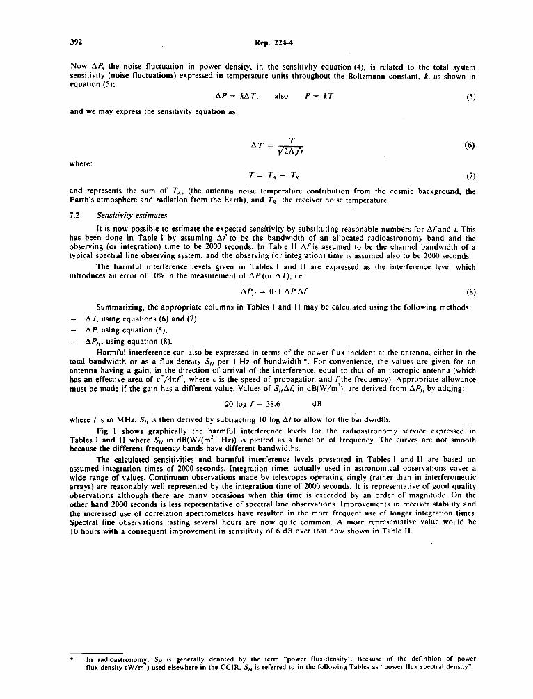
392 Rep. 224-4

Now 6P, the noise fluctuation in power density, in the sensitivity equation (4), is related to the total system sensitivity (noise fluctuations) expressed in temperature units throughout the Boltzmann constant, k, as shown in equation (5):

6P = k6T; also P= kT (5)

and we may express the sensitivity equation as:

T 6 T = V2llJi {6)

where:

(7)

and represents the sum of TA, (the antenna noise temperature contribution from the cosmic background, the Earth's atmosphere and radiation from the Earth), and Tll. the receiver noise temperature.

7.2 Sensitivity estimates

It is now possible to estimate the expected sensitivity by substituting reasonable numbers for 6f and t. This has bee'n done in Table I by assuming 6f to be the bandwidth of an allocated radioastronomy band and the observing (or integration) time to be 2000 seconds. In Table II 6f is assumed to be the channel bandwidth of a typical spectral line observing system, and the observing (or integration) time is assumed also to be 2000 seconds.

The harmful interference levels given in Tables I and 11 are expressed as the interference level which introduces an error of 10% in the measurement of tl.P(or tl.T), i.e.:

(8)

Summarizing, the appropriate columns in Tables I and II may be calculated using the following methods:

ti. T, using equations (6) and (7),

6P, using equation (5).

6PH, using equation (8).

Harmful interference can also be expressed in terms of the power flux incident at the antenna, either in the total bandwidth or as a flull·density SH per I Hz of bandwidth*. For convenience, the values are given for an antenna having a gain, in the direction of arrival of the interference, equal to that of an isotropic antenna (which has an effective area of c 2/4nf2

, where c is the speed of propagation and fthe frequency). Appropriate allowance must be made if the gain has a different value. Values of SHti.f, in dB(W Im\ are derived from ti.PH by adding:

20 log r - 38.6 dB

where fis in MHz. SH is then derived by subtracting 10 log 6fto allow for the bandwidth.

Fig. I shows graphically the harmful interference levels for the radioastronomy service expressed in Tables I and II where SH in dB(W /(m2

• Hz)) is plotted as a function of frequency. The curves are not smooth because the different frequency bands have different bandwidths.

The calculated sensitivities and harmful interference levels presented in Tables I and II are based on assumed integration times of 2000 seconds. Integration times actually used in astronomical observations cover a wide range of values. Continuum observations made by telescopes operating singly (rather than in interferometric arrays) are reasonably well represented by the integration time of 2000 seconds. It is representative of good quality observations although there are many occasions when this time is exceeded by an order of magnitude. On the other hand 2000 seconds is less representative of spectral line observations. Improvements in receiver stability and the increased use of correlation spectrometers have resulted in the more frequent use of longer integration times. Spectral line observations lasting several hours are now quite common. A more representative value would be 10 hours with a consequent improvement in sensitivity of 6 dB over that now shown in Table II.

• In radioastronom~, SH is generally denoted by the term "power nux-density". Because of the definition of power nux-density (W/m) used.elsewhere in the CCIR, SH is referred to in the following Tables as "power nux spectral density".

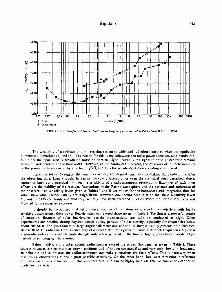
Rep. 224-4 393

-200

l•~ 19

, .. ... -210

le'' I le . " I .. ~

... ,..o .. -~ ..

~

,.., -220 .. ::c:

·' ... I

...... ·-.... A...JI •• ' _I .. - ,o

il, ,..

' ~-' .. ~ ...

r• .• ••• 4 t· ~ ~·o"

10 --41- - .. >-

:g -230

~ ~ ::!. -240

~ -250

-260

-270 0,01 0,02 0,05 0,1 0,2 0,5 2 5 10 20 50 100 200 500 1000

A: Line Frequency (GHz) B : Continuum

FIGURE I - Harmfal interference limits versus frequency as expressed in Tables I and// fort= 2000 s

The sensitivity of a radioastronomy receiving system to wideband radiation improves when the ~ndwidth is increased (equations (4) and (6)). The reason for this is the following: the noise power increases with bandwidth, but, since the signal also is broadband noise, so does the signal. Actually the signal-to-noise power ratio remains constant, independent of the bandwidth. However, as the bandwidth increases, the precision of the determination of the power levels improves (by a factor of {Kl), and thus the sensitivity is correspondingly improved.

Equations (4) or (6) suggest that one may achieve any desired sensitivity by making the bandwidth and/or the observing time, large enough. In reality, however, factors other than the statistical ones described above, sooner or later put a practical limit on the sensitivity of a radioastronomy observation. Examples of such other effects are the stability of the receiver, fluctuations in the Earth's atmosphere and the patience and endurance of the observer. The sensitivity levels given in Tables I and II use values for the bandwidth and integration time for which these other factors usually are insignificant. However, one should bear in mind that these sensitivity levels are not fundamental limits and that they actually have been exceeded in cases where the utmost sensitivity was required for a successful experiment.

It should be recognized that astronomical sources of radiation exist which may interfere with highly sensitive observations; their power flux-densities can exceed those given in Table I. The Sun is a powerful source of emission. Because of solar interference, certain investigations can only be conducted at night. Other experiments are possible during daytime except during periods of solar activity, especially for frequencies below about 200 MHz. The quiet Sun is of large angular diameter and constant in flux; it usually presents no difficulties. Below 38 MHz, radiation from Jupiter may also exceed the limits given in Table I. At such frequencies Jupiter is a sporadic radio source which emits strongly only a few per cent of the time at highly predictable periods. These periods of emission can be avoided.

Below I GHz, many other cosmic radio sources exceed the power flux-densities given in Table I. These sources however, are generally at known positions and of known constant flux and vary only slowly in frequency. In principle and in practice the radioastronomer can make corrections for their effects. This is necessary when performing observations at the highest possible sensitivity. On the other hand, low level terrestrial interference normally has an unknown position, flux and spectrum, and can be highly time variable, so corrections cannot be made for its effects.

TABLE I - Sensitivities and harmful interference levels for radioastronomy continuum observations with 2000 second integration time

-System sensitivity

Harmful interference levels (noise fluctuations)

Nominal Centre Assumed Minimum Receiver

frequency frequency(') bandwidth antenna noise noise temperature temperature Power

Temperature spectral Input Power Power flux

density power flux spectral density

f. J; ::.~ ;~ ;~ t:.T AP AP9 S91!>.JA Sn (Mi'Iz) (Mliz) (M z) (mK) (dB(W/Hz)) (dBW) (dB(W/m2)) (dB(W/(m' · Hz)))

(l) (2) (3) (4) (5) (6) (7) (8) (9) (10)

20 21.860 0.020 30000 100 3 365.00 -223 -190 -202 -245 40 38.000 0.500 6000 100 136.00 -237 -190 -197 -254 80 73.800 1.600 1000 100 13.75 -247 -195 -196 -258

150 152.000 3.000 200 100 2.74 -253 -199 -195 -259 327 325.300 6.600 40 100 0.86 -259 -201 -189 -258 408 408.050 3.900 25 100 1.00 -259 -203 -189 -255 610 611.000 . 6.000 15 100 0.74 -260 -202 -185 -253

1420 1413.500 27.000 10 20 0.09 -269 -205 -180 -255 2700 2695.000 10.000 10 20 0.15 -267 -207 -177 -247 5000 4 995.000 10.000 10 20 0.15 -267 -207 -171 -241

10650 10690 100 12 20 0.05 -272 -202 -160 -240 15 350 15 375 50 15 30 0.10 -269 -202 -156 -233 23 800 23 800 400 15 50 0.05 -271 -195 -146 -233 31400 31400 200 18 100 0.13 -267 -194 -143 -226

90000 89000 6000 30 150 0.04 -273 -185 -125 -223 135 000 135000 10000 40 ISO 0.03 -274 -184 -120 -220 235000 235000 10000 35 200 0.04 -273 -183 -114 -214

(') Calculation of harmful interference levels is based on the centre frequency shown in this column although not all regions have the same allocations. Note. - If an integration time of 15 minutes, one hour, two hours, five hours or ten hours is used, the relevant values in the Table should be varied by + l. 7, -1.3, -2.8, -4.8 or -0.3 dB

respectively. ·

f

" ~

"!II w

t

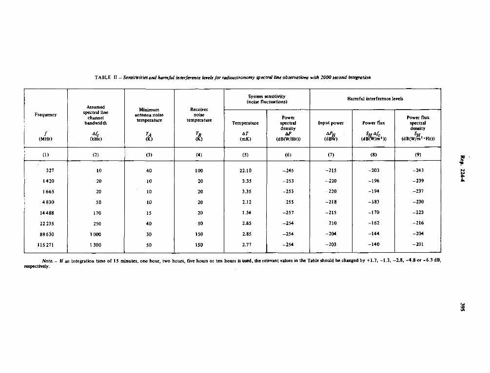
TABLE II - Sensitillities and hannful interference levels for radiCHZstronomy spectral line obseniations with 2000 second integration

System sensitivity Harmful interference levels (noise fluctuations)

Assumed Minimum Receiver Frequency spectral line antenna noise noise

channel Power Power flux bandwidth

temperature temperatw:e Temperature spectral Input power Power flux spectral

density density f ilfc ~) ff) ilT ill' ill'H ~~ilfc SH

{MHz) (kHz) (mK) (dB(W/Hz)) (dBW) (dB /m")) (dB(W/m" ·Hz))

(I) (2) (3) {4) (5) (6) (7) (8) (9)

327 10 40 100 22.10 -245 -215 -203 -243

1420 20 10 20 3.35 -253 -·220 -196 -239

1665 20 10 20 3.35 -253 -220 -194 -237

4830 50 10 20 2.12 -255 -218 -183 -230

14488 170 15 20 1.34 -257 -215 -170 -223

22 235 250 40 50 2.85 -254 -210 -162 -216

88630 l 000 30 150 2.85 -254 -204 -144 -204

115 271 1300 50 ISO 2.77 -254 -203 -140 -201

Note. - If an integration time of IS minutes, one hour, two hours, five hours or ten hows is used, the relevant values in the Table should be changed by +1.7, -1.3, -2.8, -4.8 or -6.3 dB, respectively.

,, "' "!='

f

1i

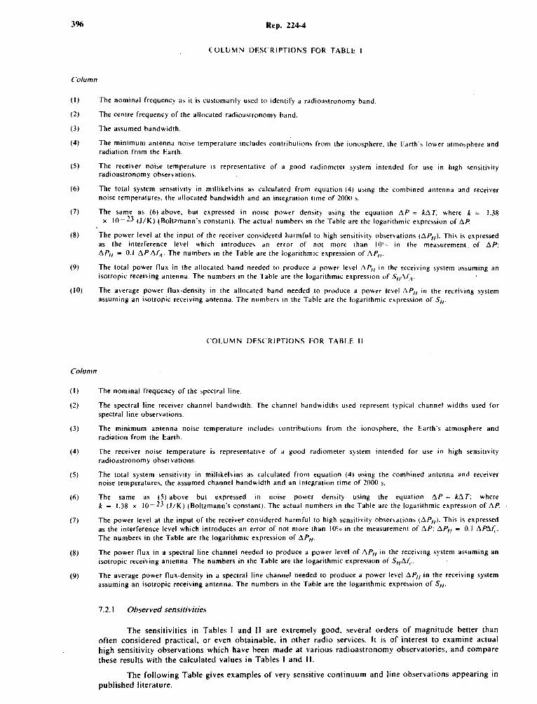
396 Rep. 224-4

COLUMN DESCRIPTIONS FOR TABLE I

Column

(I) The nominal frequency as it is customarily used to identify a radioastronomy band.

(2) The centre frequency of the allocated radioastronomy band.

(3) The assumed bandwidth.

(4) The minimum antenna noise temperature includes contributions from the ionosphere. the Earth'' lower atmosphere and radiation from the Earth.

(5) The receiver noise temperature is representative of a good radiometer system intended for use in high sensitivity radioastronomy observations.

(6) The total system sensitivity in millikelvins as calculated from equation (4) using the combined antenna and receiver noise temperatures. the allocated bandwidth and an integnllion time of 2000 s.

(7) The same as (6) above. but expressed in noise power density using the equation !lP = k!l T. where k = 1.38 x 10-23 (J/K) (Boltzmann's constant). The actual numbers in the Table are the logarithmic expre,sion of l'lP.

(8) The power level at the input of the receiver considered harmful to high sensitivity observations (/l,.P11 ). This is expressed as the interference level which introduces an error of not more than IO''" in the measurement of l'lP: 6P11 - 0.1 !lP l'lf4 . The numbers in the Table are the logarithmic expression of l'lP11 .

(9) The total power nux in the allocated band needed to produce a power level l'lP11 in the receiving system assuming an isotropic receiving antenna. The numbers in the Table are the logarithmic expression of Sfll'lf.1.

( 10) The average power nux-density in the allocated band needed to produce a power level l'lP11 in the receiving system assuming an isotropic receiving antenna. The numbers in the Table are the logarithmic expression of SH.

COLUMN DESCRIPTIONS FOR TABLE II

Column

(I) The nominal freqliency of the spectral line.

(2) The spectral line receiver channel bandwidth. The channel bandwidths u~ed represent typical channel widths used for spectral line observations.

(3) The minimum antenna noise temperature include, contributions from the iono,phere, the Earth's atmosphere and radiation from the E:arth.

(4) The receiver noise temperature is representative of a good radiometer system intended for use in high sensitivity radioastronomy observations.

(5) The total system sensitivity in millikelvins a' calculated rrom equation (4) using the combined antenna and receiver noise temperatures, the assumed channel bandwidth and an integration time of 2000 s.

(6) The same as (5) above but expressed in noise power density using the equation !lP = k!l T: where k = 1.38 x 10-23 (J/KJ (Boltzmann's constant). The actual numbers in the Table are the logarithmic expression of 6P.

(7) The power level at the input of the receiver considered harmful to high sensitivity obsenations (6P11 ). This is expressed as the interrerence level which introduces an error or not more than 10°10 in the measurement of l'lP: l'lPfl = 0.1 !'i.Pllf.." The numbers in the Table are the logarithmic expression of !lPfl.

(8) The power nux in a spectral line channel needed to produce a power level or !lPfl in the receiving system assuming an isotropic receiving antenna. The numbers in the Table are the logarithmic expression of Sfll'lf.. ..

(9) The average power nux-density in a spectral line channel needed to produce a power level 6P11 in the receiving system assuming an isotropic receiving antenna. The numbers in the Table are the logarithmic expression of 5 11 .

7.2.1 Observed sensitivities

The sensitivities in Tables I and 11 are extremely good, several orders of magnitude better than often considered practical, or even obtainable, in other radio services. It is of interest to examine actual high sensitivity observations which have been made at various radioastronomy observatories, and compare these results with the calculated values in Tables I and II.

The following Table gives examples of very sensitive continuum and line observations appearing in published literature.

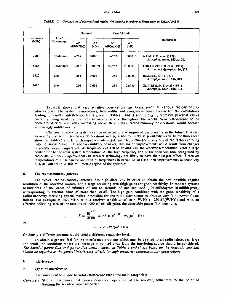
Rep. 224-4 397

TABLE Ill - Compariwn of obseniational results with harmful interference limits given in Tabler I and II

Observed Harmful limit

Frequency Line/ References (MHz) Continuum 4.1' liT tJ.P tiT (dB(W/Hz)) (mK) (dB(W/Hz)) (mK)

2700 Continuum -269 0.0001 -267 0.00015 WADE,C.M.tta/. (1971) Astrophys. Journ. 163, LlOS.

8785 Continuum -265 0.00024 "'-267 .. 0.0001 FOMALONT, E.B. et al. (1975) Astron. and Astrophys. 36, 273.

1420 Line -254 0.003 -253 0.0035 BIGNELL, R.C. (1973) Astrophys. Journ. 186, 889.

1690 Line -256 0.002 -253 0.0035 GOTTESMAN, S. et al. (1971) Asrrophys. Journ. 168, 131.

Table III shows that very sensitive observations are being made at various radioastronomy observatories. The system temperatures, bandwidths and integration times chosen for the calculations leading to harmful interference limits given in Tables I and II and in Fig. I, represent practical values currently being used by the radioastronomy service throughout the world. Were interference to be encountered with intensities increasing above these limits, radioastronomy observations would become increasingly untrustworthy.

Changes in receiving systems can be expected to give improved performance in the future. It is safe to assume that within ten years observations will be made routinely at sensitivity levels better than those shown in Tables I and II. Such improvements might result from changes in any one of the factors entering into Equations 6 and 7. It appears unlikely however, that major improvements could result from changes in receiver noise temperature. At frequencies of 150 MHz and less, the receiver temperature is not a large contributor to the total system temperature. At the high frequency end of the spectrum now being used by radio astronomers, improvements in receiver technology are likely to have their largest effect. If receiver temperatures of 10 K can be achieved at frequencies in excess of 30 GHz then improvements in sensitivity of 6 dB will result in this millimetric region of the spectrum.

8. The radioastronom)· ?ntenna

The typical radioastronomy antenna has high directivity in order to obtain the best possible angular resolution of the observed sources, and a large collecting area (high gain) for good sensitivity. In modern systems beamwidths of the order of minutes of arc to seconds of arc are used (JOO millidegrees-JO millidegrees), corresponding to antenna gains of more than 70 dB. The high gain combined with the good sensitivity of a radioastronomy receiving system makes it possible for the radio astronomer to observe very faint power fluxes indeed. For example at 1420 MHz, with a receiver sensitivity of 10- 21 W/Hz (-270 dB(W/Hz)) and with an effective collecting area of the antenna of 4000 m1 (61 dB gain), the detectable power flux density is:

10-27 -31

S = 4000

= 2.5 x IO W/(m 2 • Hz)

or:

- 306 dB(W /(m1. Hz)).

Obviously a different antenna would yield a different sensitivity level.

To obtain a general feel for the interference problems which may be applied to all radio telescopes, large and small, the conditions where the telescope is pointed away from the interfering source should be considered. The harmful power flux and power flux-density shown in Tables I and II are based on the isotropic case and should be regarded as the general interference criteria for high sensitivity radioastronomy observations

9. Interference

9.1 Types of interference

It is convenient to divide harmful interference into three main categoric~:

Category I: Strong interference that causes non-linear operation of the receiver, sometimes to the point of harming the sensitive input amplifier.

398 Rep. 224-4

Fortunately, this type of interference is rare and unlikely to be caused by normal transmissions. However, rad~r .transmitters in I.ow flying aircraft are capable of physically damaging the electronics of a radioastronomy receiving system. Typically a power level at the radiometer input of 0.1 W would burn out the varactor in a parame~ric amplifier. Thi.s corresponds to a power flux of I 0 W Im' (I 0 dB(W lm 2)) at 1400 MHz, if the interfering source 1s outside the main beam of the antenna. The corresponding power flux-density, assuming a bandwidth of 27 MHz (1400 to 1427 MHz) would be 3.7 x 10- 1Wl(m'. Hz) or -64 dB(Wl(m 2

• Hz)). If the antenna is accidentally pointed at such a strong interference source, the power flux-density that could burn out the input varactor must be reduced by the gain of the antenna.

Category 2: Relatively strong interference which is easy to recognize.

Usually this is the case if the interference power is stronger than the noise power in the radiometer input. This type of interference is fatal to observations, and there is no doubt that it is interference. There is no choice but to discard the data. Typically, interference power fluxes above -110 dB(W/m2

) belong in this category. With an assumed bandwidth of 27 MHz (the 1413.5 MHz band), the corresponding power flux-density is -184 dB(W/(m2

• Hz)).

Category 3: Very low-level interference with a very low interference to noise ratio (less than - 20 dB) that cannot be recognized.

The long integration times required to bring the wanted signal out of the noise will mask the characteristic features of the interfering signal. It cannot be recognized as interference and erroneous data result; this type of low-level interference is therefore particularly harmful. Furthermore, because the radio astronomer cannot determine by examination of the data that he has encountered interference, there is no possibility of identifying the source.

9.2 Interference reduction techniques

A number of techniques designed to reduce the effects of interference can be tried by the radio astronomer. Some of these are obvious and straightforward, and some are clever. complicated and often time consuming. They all suffer from the problem of being of limited usefulness. In general, the employment of interference reduction techniques leads to the need for more observing time.

9.2.1 Filtering techniques.

Unwanted signal energy outside the observed band is rejected in the radioastronomy receiver by using bandpass filters. Normally, when the interfering signals are of low intensity and do not cause non-linear operation anywhere in the system, limiting the observed passband by Al filter in the IF channel is useful. Since the IF frequencies are relatively low, typically between I 00 to 300 MHz, relatively steep skirt selectivity is possible. However, limiting the observing band decreases the sensitivity of the system which is proportional to {M: Filtering in the radiometer input is also used, particularly when the potentially interfering signals are strong. Again decreased sensitivity is the result, both because of the narrower bandwidth and because of the insertion loss of the filter which, when inserted in the receiver input, adds to the loss and the noise temperature of the system. Since the filtering takes place at the observing frequency, adequate skirt selectivity may be a problem. Typically, about 75% of an allocated band remains available after a reasonable IF filtering (see Report 696) which corresponds to a sensitivity loss of about 13%. If input filtering is needed, sensitivity reduction of a factor of 2 or more could be expected.

In order to obtain 100 dB reduction of the midband response at the band edge of the radio­astronomy ban~, one needs three or more 8-section filters in the IF channel. Although such a filter system is feasible, there are important phase considerations to be taken into account when observing with an antenna array or interferometer. This makes it questionable whether filtering really is a· viable general solution to the band edge interference problem. Bandpass filters do not, of course, alleviate the in-band interference problem.

9.2.2 Observing techniques

It is possible, and often necessary, to reduce the effect of interference by using special observing techniques. One possibility is to repeat the observation several times, with the assumption that the interference is present only occasionally. It is also useful to move the telescope on a,nd off the source during an observing run, assul)'ling that the interference is present all the time. Both methods are of limited usefulness, because of the assumptions one has to make of the behaviour of the celestrial source as well as of the interference. They also increase the required observing time by a sizeable factor. Furthermore, the

Rep. 224-4 399

technique of repeating the observations is not very useful in the case of sources of variable intensity, as it is not possible to distinguish between variations in the interference and in intrinsic variations in the source. The on/off technique is not useful for observations of extended astronomical objects, such as the cosmic background, since there is no region of the sky which can be considered off-source. An assumption that the intensity of the interference is constant must also be made. This is not generally true; often the interference varies in intensity with time and in a complicated way across the frequency band.

9.2.3 Data processing techniques.

After-the-fact reduction of the effects of very low-level interference is of very limited usefulness in radioastronomy. One reason for this is that in order to detect power at a very low level, long integration times, which mask the identifying characteristics of the interfering signals, have to be used. The added power caused by the interference is then no longer distinguishable from the random noise one is looking for. It might be possible, in some special cases such as pulsed radar interference where the characteristics of the interfering signals are also accurately known, to process the data in a way that might reduce the effect of the interference.

Continuum observations, which require a large bandwidth in order to achieve good sensitivity, can be made by a receiver covering the desired bandwidth with a number of contiguous channels (a spectral line receiver). The spectral information can then be used to identify a narrow interfering signal. However, for interference covering a bandwidth comparable to the continuum bandwidth observed, this technique is not useful.

In very special and rare cases if the characteristics of the wanted signal are known, this fact can be used to separate it from the interference and noise. However, for the general case of radioastronomy observations, there seems not to be any useful data processing technique that may be used to identify and reduce interference.

9.3 Interference and long baseline interferometers

High resolution observations require the use of interferometers or arrays of antennae with wide spacings between their elements. Each antenna may be subject to different interference conditions. In the extreme case of very long base-line interferometer (VLBI), the interference may affect only one antenna of the system. This may reduce the effect of interference by a small factor. On the other hand, it should be noted that VLBI experiments involve sophisticated data reduction and use of very distant antennae with consequent co-ordination problems. Interference affecting only one antenna may invalidate a whole observation. This leads to the need for world-wide protection of VLBI observations.

REFERENCES AND BIBLIOGRAPHY

COHEN, M. H. [1969) High resolution observations of radio sources. Annual Re~. of Astron. and Astrophys., 7, 619-664.

ELLIS, G. R. A. and HAMILTON, P.A. (1966) Astrophys. Journ., 143, 227.

EWEN, H. I. and PURCELL, E. M. (1951) Nature, 1611, 356.

HEWISH, A., BELL, S. J., PILKINGTON, J. D. H., SCOTI, P. F. and COLLINS, R. A. (1968) Observations of a rapidly pulsating radio source. Nature, 217, 709-713.

JANSKY, K. G. [1935) Pro,-. IRE, 23, 1158.

KRAUS, J. D. (1966) Radio Astronomy, McGraw Hill, New York, USA.

LILLEY, A. E. and PALMER, P. [1968) Tables of radio frequency recombination lines. Astrophys. Journ., Suppl. Series No. 144, 16, 143-174.

RADHAKRISHNAN, V. (1969) Fifteen months of pulsar astronomy. Proc. Astron. Soc. of Australia, I, 254-263.

ROBERTS, J. A. [ 1963) Radio emission from the planets. Planet. and Space Science, 11, 221.

SNYDER, L. E., BUHL, D., ZUCKERMAN, B. and PALMER, P. (1969) Microwave detection of interstellar formaldehyde. Phys. Rev. Letters, 22, 679.

VERSCHUUR, G. L. (1969) Measurements of magnetic fields in interstellar clouds of neutral hydrogen. Astrophys. Journ., 156, 861-874.

WEINREB, S., BARRETT, A.H., MEEKS, M. L. and HENRY, J.C. [1963] Nature, 200, 829.

WILD, J.P., SMERD, S. F. and WEISS, A. A. (1963) Solar bursts. Annual Rev. of Astron. and Astrophys., 1, 291.

CCJR Document

(1971): Report of the CCIR Special Joint Meeting, Geneva, 1971, Chapter 3, Table 3.3-JV.

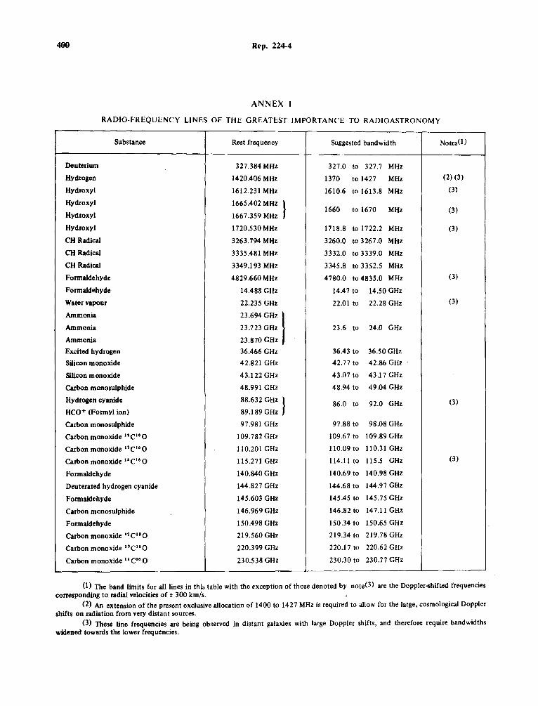
400 Rep. 224-4

ANNEX I

RADIO-FREQUENCY LINES OF THE GREATEST IMPORTANCE TO RADIOASTRONOMY

Substance Rest frequency Suggested bandwidth NotesO)

Deuterium 327.384 MHz 327.0 to 327.7 MHz

Hydrogen 1420.406 MHz 1370 to 1427 MHz (2) (3)

Hydroxyl 1612.231 MHz 1610.6 to 1613.8 MHz (3)

Hydroxyl 1665.402 MHz } Hydroxyl 1660 to 1670 MHz (3)

1667 .359 MHz

Hydroxyl 1720.530 MHz 1718.8 to 1722.2 MHz (3)

CH Radical 3263.794 MHz 3260.0 to 3267.0 MHz

CH Radical 3335.481 MHz 3332.0 to 3339.0 MHz

CH Radical 3349.193 MHz 3345.8 to 3352.5 MHz

Formaldehyde 4829 .660 MHz 4780.0 to 4835.0 MHz (3)

Formaldehyde 14.488 GHz 14.47 to 14.50 GHz

Water vapour 22.235 GHz 22.01 to 22.28 GHz (3)

Ammonia 23.694 G"' I

Ammonia 23.723 GHz 23.6 to 24.0 GHz

Ammonia 23.870 GHz

Excited hydrogen 36.466 GHz 36.43 to 36.50 GHz

Silicon monoxide 42.821 GHz 42.77 to 42.86 GHz

Silicon monoxide 43.122 GHz 43.07to 43.17 GHz

Carbon monosulphide 48.991 GHz 48.94 to 49.04 GHz

Hydrogen cyanide 88.632 GHz } 86.0 to 92.0 GHz (3) Hco+ (Formyl ion) 89.189GHz

Carbon monosulphide 97 .981 GHz 97 .88 to 98.08 GHz

Carbon monoxide 12C11 0 109.782 GHz 109.67 to 109.89 GHz

Carbon monoxide "C"O 110.201 GHz 110.09 to 110.31 GHz

Carbon monoxide 11 C16 0 115.271 GHz 114.11 to 115.5 GHz (3)

Formaldehyde 140.840 GHz 140.69 to 140.98 GHz

Deuterated hydrogen cyanide 144.827 GHz 144.68 to 144.97 GHz

Formaldehyde 145.603 GHz 145.45 to 145.75 GHz

Carbon monosulphide 146.969GHz 146.82 to 147.11 GHz

Formaldehyde 150.498 GHz 150.34 to 150.65 GHz

Carbon monoxide 11 C18 0 219.560GHz 219.34to 219.78 GHz

Carbon monoxide ''C"O 220.399 GHz 220.17 to 220.62 GHz

Carbon monoxide 11 C'6 0 230.538 GHz 230.30 to 230.77 GHz

(1) The band limits for all lines in thii; table with the exception of those denoted by note(3) are the Doppler-shifted frequencies corresponding to radial velocities of ± 300 km/s.

(2) An extension of the present exclusive allocation of 1400 to 1427 MHz is required to allow for the large, cosmological Doppler shifts on radiation from very distant sources.

(3) These line frequencies are being observed in distant galaxies with large Doppler shifts, and therefore require bandwidths widened towards the lower frequencies.

APPENDIX B

CCIR REPORTS ON DEEP-SPACE RESEARCH (Reports 365-3 and 685)

144 Rec. 365-3

RECOMMENDATION 365-3 *

FREQUENCIES, BANDWIDTHS AND PROTECTION CRITERIA FOR MANNED AND UNMANNED DEEP-SPACE RESEARCH

(Question 1-112)

( 1963 - 1966 - 1974 - 1978) The CCIR,

CONSIDERING

(a) that suitable operating frequencies, required radio-frequency bandwidths, and limiting interference criteria for deep-space manned and unmanned research telecommunication links are determined by the technical considerations set forth in Reports 536-1, 683 and 685.

(b) that' cosmic noise and- man-made noise militate against the use of frequencies lower than 100 MHz and that atmospheric noise and absorption allow the use of only particular frequency bands at frequencies much higher than 10 GHz;

(c) that some high precision tracking techniques required for guidance of spacecraft to the Moon and the planets and for manoeuvres in their vicinity result in a preference for several widely separated frequencies above I GHz;

(d) that two-way communication is required for all deep-space missions, and is vital for manned deep-space missions;

(e) that manned deep-space missions require in particular two-way voice and also television as aids to command and control, guidance navigation and other telecommunication functions:

(I) that for most deep-space missions the typical operating noise temperature of earth station receivers, operating at frequencies in the 2 GHz region will be 16 K, equivalent to -217 dB(W/Hz), in the 8 GHz region will be 23 K, equivalent to - 215 dB(W /Hz), and in the 15 GHz region will be 33 K, equivalent to -213 dB(W/Hz), with design margins of less than 6 dB; and that for reception at frequencies less than I GHz cosmic noise increases the system noise temperature approximately as the inverse of the square of the frequency;

(g) that the typical operating input noise temperature of a receiver in a deep-space station operating at frequencies in the 2 GHz region will be 600 K, equivalent to -201 dB(W/Hz), in the 7 GHz region will be 800 K, equivalent to -200 dB(W/Hz), and in the 15 GHz region will be 1100 K, equivalent to -198 dB(W/Hz), with design margins of less than 6 dB; and that for reception at frequencies less than 300 MHz, cosmic noise increases the system noise temperature approximately as the inverse of the square of the frequency:

(h) that, at frequencies higher than 4 GHz, water vapour in the atmosphere can produce significant degradation in the quality of deep-space communications;

(j) that typical deep-space systems will use directional antennae both on the Earth and on the spacecraft. These antennae will have a surface precision of between 0.24 mm and 5 mm r.m.s., regardless of diameter, so that frequencies between I and 20 GHz will generally be more suitable for efficient transmission;

(k) that Doppler shifts can be of the order of I x I 0-4 of the carrier frequency;

(/) that interruptions in communications which aggregate to more than five minutes on any one day without prior planning, could seriously affect the success of the mission;

(m) that real-time television from the lunar surface is practical with frame rates, resolutions, and qualities comparable to terrestrial television, and that photographic facsimile from the nearer planets is similarly practical;

(n) that it is practical and desirable to effect telemetering, data transmission, and tracking functions on the same space-to-Earth link, and telecommand and tracking functions on the same Earth-to-space link;

(o) that to effect precision tracking, a pair of coherently-related Earth-to-space and space-to-Earth frequencies with a separation of at least 7% of the higher frequency in any one band (e.g. pairs near 2 GHz, 8 GHz an<I the region of 15 GHz) is required, and that for more accurate correction for effects of charged particles on space propagation delays, simultaneous use of space-Earth links with coherent frequencies in two or more of these bands is required;

(p) that to enable precision tracking corrections and to allow both low-rate weather-immune emergency communications, and high-rate primary communications, both Earth-to-space and space-to-Earth communications are desirable on two or more widely separated frequency bands (e.g. 2 GHz, 8 GHz and near 15 GHz);

(q) that the angular spacings of the Moon and the planets are often such that the same frequency may be used for probes at different celestial coordinates, but that different spacecraft in the vicinity of the same coordinates or in the antenna beamwidth may require different frequencies;

This Recommendation is brought to the attention of Study Groups I, 4, 7, 8, 9, 10 and 11.

Rec. 365-3 145

(r) that geographical separations which permit sharing between terrestrial services and deep-space research operations are typically several hundreds of kilometres, and may be greater than 500 km in the absence of terrain shielding; that separations of this magnitude are not readily obtainable in many parts of the world; and that the spacecraft are visible over large areas of the Earth;

(s} that considerable difficulties can be expected when sharing frequencies between deep-space research operations and other services, due to the technical problems of furnishing the required protection against both terrestrial and near-Earth satellite transmissions,

UNANIMOUSLY RECOMMENDS

I. that frequencies for deep-space manned and unmanned telecommunication links be located in the frequency band between I 00 MHz and 30 GHz, with additional links for use during near-Earth and recovery phases of manned space-flights in the frequency bands below 25 MHz, in accordance with the following guidelines:

I. I frequencies in the HF range below 25 MHz are technically suitable for two-way voice and other comm,unications during manned mission near-Earth and recovery phases;

1.2 the band between 100 MHz and I GHz is generally more suitable for narrow-band telemetering, tracking, telecommand and voice from launch to intermediate distances;

1.3 the band between I GHz and 6 GHz is generally more suitable for wideband telemetering, precision tracking, telecommand, voice and television from launch to extreme distances;

1.4 the band above 6 GHz is generally more suitable for very wideband telemetering, very precise tracking and television at various distances;

1.5 that special consideration should be given to the availability of coherently related frequencies, spaced at 7% or more of the higher frequency in the bands above I GHz, and to the availability of frequencies in three bands, widely separated in frequency, such as the 2 GHz, 8 GHz and 15 GHz regions for precision tracking systems;

2. that spectrum space of the order of 2 to 4 MHz per link (due account being taken of the dependency of the radio-frequency bandwidth on the type of modulation used) is technically suitable for the transmission of wideband information for lunar flights.

3. that spectrum space of the order of 2 to 6 MHz per link is technically suitable for the transmission of wideband signals for precision two-way ranging;

4. that bandwidths of the order of 40 to 400 MHz per link are technically suitable for the transmission of very wideband signals for very precise two-way tracking;

5. that tracking be time-multiplexed with lunar television or planetary facsimile where practicable;

6. that where practicable, frequencies be shared among deep-space probes with different launch periods and different ceJestial coordinates, but not generally with spacecraft with the same celestial coordinates;

7. that the protection criteria for earth stations be established as follows: the total time during which the power spectral density of noise-like interference, or the total power of CW-type interference in any single band and all sets of bands I Hz wide, is greater than - 222 dB(W /Hz) in the 2 GHz region, -220 dB(W /Hz) in the 8 GHz region, and -218 dB(W/Hz) in the 15 GHz region, at the input terminals of the receiver, shall not exceed an aggregate of five minutes on any one day without prior planning; for frequencies below I GHz, the permissible interference power level may be increased at the rate of 20 dB per decreasing frequency decade;

8. that the protection criteria for space stations be established as follows: the total time during which the power spectral density of noise-like interference or the total power of CW-type interference in any single band and all sets of bands 1 kHz wide, is greater than -171 dB(W/kHz) in the 2 GHz region, -170 dB(W/kHz) in the 7 GHz region and -168 dB(W/kHz) in the 15 GHz region, at the input termifl;lls of the receiver, shall not exceed an aggregate of five minutes of any one day; for frequencies less than 300 MHz, the permissible interference may be increased at the rate of 20 dB per decreasing frequency decade;

9. that, when necessary for emergency purposes, manned deep-space flights use the recognized distress frequencies in accordance with the Radio Regulations;

10. that a deep-space research service cannot share Earth-to-space bands with:

10.1 receiving aeronautical mobile stations,

I 0.2 receiving satellite stations, and

I 0.3 transmitting terrestrial stations and earth stations utilizing high average e.i.r.p.; for example, transmitting trans-horizon stations, and transmitting fixed satellite earth stations.

When coordination is practicable, sharing is feasible with other stations of all services. In some cases, coordination distances may be unacceptably great;

146 Rec. 365-3, 364-3

11. that a deep-space research service cannot share space-to-Earth bands with:

I I.I transmitting aeronautical mobile stations, and

11.2 transmitting satellite stations.

When coordination is practicable, sharing is feasible with other stations of all services. In some cases, coordination distances may be unacceptably great.

RECOMMENDATION 364-3 *

TELECOMMUNICATION LINKS FOR MANNED AND

UNMANNED NEAR-EARTH RESEARCH SATELLITES

Frequencies, bandwidths and criteria for protection from interference

(Questions 1812 and 2212)

(1963 - 1966 - 1970 - 1978) The CCIR,

CONSIDERING

(a.) that suitable operating frequencies, required radio-frequency bandwidths, and limiting interference criteria for near-Earth satellite telecommunication links are determined by the technical considerations set forth in the appropriate Reports;

(b) that, based on past experience, it is expected that of the order of 100 active research near-Earth satellites may be h orbit simultaneously;

(c) that two-way communication is required for many near-Earth missions, and is vital for manned missions;

(d) that various radio-frequency bands are suitable for near-Earth satellite telecommunication links, and that the variety of functions and the conditions under which they must be performed divide this region into the following suitable regions: below I GHz, I to 6 GHz, 6 to 10 GHz, and IO to 30 GHz;

(e) that telemetering data lir.ks typically require radio-frequency bandwidths ranging from 10 kHz to 20 MHz per link in the frequency range from 100 MHz to 30 GHz, with a bandwidth of 10 kHz in the lower portion, and up to 20 MHz in the upper portion;

(f) that tracking links typically require radio-frequency bandwidths ranging from 10 kHz to 100 MHz per link in the frequency range from 100 MHz to 15 GHz with bandwidths of 10 kHz in the lower portion and up to 100 MHz in the upper portion of this range, the latter being required for high precision two-way, coherent, range and range rate systems;

(g) that voice links typically require radio-frequency bandwidths ranging from 3 kHz to 45 kHz per link;

(h) that wideband data and television links typically require radio-frequency bandwidths within the range 50 kHz to 300 MHz in the frequency range from 100 MHz to 30 GHz, with preference for 50 kHz in the lower portion and 300 MHz in the upper portion of li1is range;

(j) that the operating noise temperatures of earth-station telemetering and tracking receiving systems usually range from 30 K above I GHz to 3000 Kat 100 MHz (equivalent lo -214 dB(W/Hz) and -194 dB(W/Hz));

(k) that earth-station antenn.le for satellite communication do not operate at elevation angles less than 5", except for initial acquisition;

(/) that typical operating noise temperatures for receivers in near-Earth research spacecraft are approximately 600 K ( - 171 dB(W /kHz)), but that measures can be taken to protect the spacecraft receiving system against interference approximately I 0 dB greater than thi~. noise level;

(m) that telecommand requirements can normally he satisfied by one data link channel per craft with radio-frequency bandwidths ranging from 10 kHz at 100 MHz to 500 kHz at 15 GHz, largely determined by the Doppler shift which may be of the order of I x 10- 4 of the carrier frequency;

(n) that coding techniques and the future use of narrow-beam antennae may make possible the control of several crafts using the same radio-frequency telecommand channel;

(o) that circuit design in spacecraft for high precision coherent tracking systems dictate that two frequencies be used, spaced by at least 6% of the higher one;

* This Recommendation is brought to the attention of Study Groups I, 4, 7, 8, 9, 10 and 11.

Rec. 364-3, Rep. 684 147

(p) that, for some frequency sharing situations between near-Earth research satellites and certain representative terrestrial services, separations of several hundreds of kilometres between the earth terminals may be required and that, in many parts of the world, separations of this magnitude are not readily attainable; (q) that frequency sharing among near-Earth research satellites is desirable and feasible; (r) that difficulties can be expected when frequencies are shared between near·Earth research satellites and stations in other Services, due to the technical problems of furnishing the required protection against terrestrial Services,

UNANIMOUSLY RECOMMENDS

I. that the range below I GHz is technically suitable for near-Earth research satellites, with each satellite using radio-frequency bandwidths varying from 10 to 500 kHz per link, for accomplishing telemetering, wideband data transmission, tracking, telecommand and voice functions; 2. that the range between I GHz and 6 GHz is technically suitable for near-Earth research satellites, with each satellite using radio-frequency bandwidths varying from 500 kHz to 4 MHz per link, for accomplishing telemetering, wideband data transmission, tracking, telecommand, voice and television functions; 3. that the range between 6 and 10 GHz is technically suitable for near·Earth research satellites, with each satellite using radio frequency bandwidths varying from 500 kHz to 20 MHz per link, for accomplishing telemetering, wideband data transmission, tracking, telecommand, voice and television functions; 4. that the range between IO GHz and 30 GHz is technically suitable for near-Earth research satellites, with each satellite using radio frequency bandwidths ranging from 1 MHz to 300 MHz per link, for accomplishing telemetering, wideband data transmission and television functions; 5. that high frequencies below about 25 MHz are technically suitable for two-way voice communication during manned-mission near-Earth and recovery phases; 6. that, when necessary, for emergency purposes in manned near-Earth missions, the recognized distress frequencies be used in accordance with the Radio Regulations; 7. that consideration be given to the availability of coherently related frequencies spaced by more than 6% of the higher frequency for precision tracking systems;

, 8. that frequency sharing be accomplished to the maximum extent feasible among near-Earth research satellites; 9. that the protection criterion for earth receiving stations be established as follows: for frequencies greater ~han I GHz and up to at least IO GHz, the total time for which the power spectral density of noise-like interference or the total power of CW-type interference in any single band and all sets of bands 1 Hz wide is greater than -220 dB(W/Hz) at the input terminals of the receiver, shall not exceed 5 minutes per day, for manned research missions (O.lo/o of the time being permissible for other near-Earth research missions); for frequencies less than I GHz, the permissible interference may be increased at the rate of 20 dB per decreasing frequency decade; 10. that the protection criterion for receivers in spacecraft be established as follows: for frequencies greater than 300 MHz and up to at least 10 GHz, the total time during which the power spectral-density of noise-like interference or the total power of CW-type interference in any single band or all sets of bands I kHz wide is greater than - 171 dB(W /kHz) at the input terminals of the receiver, shall not exceed 5 minutes per day for manned research missions ( - 161 dB(W /kHz) during a maximum of 0.1 % of the time being permissible for other near-Earth research missions); for frequencies less than 300 MHz, the permissible interference may be increased at the rate of 20 dB per decreasing frequency decade; 11. that note be taken of the difficulties to be expected in frequency sharing between near-Earth research satellites and stations in other services.

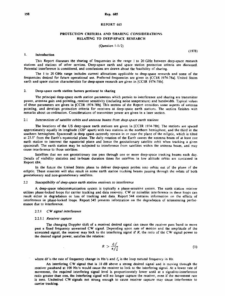
158 Rep. 685

REPORT 685

PROTECTION CRITERIA AND SHARING CONSIDERATIONS RELATING TO DEEP-SPACE RESEARCH

(Question 1-1 /2)

(1978) I. Introduction

This Report discusses the sharing of frequencies in the range I to 20 GHz between deep-space research stations and stations of other services. Deep-space earth and space station protection criteria are discussed. Potential interference is considered, and conclusions are drawn about the feasibility of sharing.

The I to 20 GHz range includes current allocations applicable to deep-space research and some of the frequencies desired for future operational use. Preferred frequencies are given in [CCIR 1974-78a). United States earth and space station characteristics for deep-space research are given in [CCIR 1974-78b).

2. Deep-space earth station factors pertinent to sharing

The principal deep-space earth station parameters which pertain to interference and sharing are transmitter power, antenna gain and pointing, receiver sensitivity (including noise temperature) and bandwidth. Typical values of these parameters are given in [CCIR 1974-78b). This section of the Report considers some aspects of antenna pointing, and develops protection criteria for receivers at deep-space earth stations. The section finishes with remarks about co-ordination. Considerations of transmitter power are given in a later section.

2.1 Intersections of satellite orbits and antenna beams from deep-space earth stations

The locations of the US deep-space earth stations are given in [CCIR 1974-78b). The stations are spaced approximately equally in longitude (120° apart) with two stations in the northern hemisphere, and the third in the southern hemisphere. Spacecraft in deep space currently remain in or near the plane of the ecliptic, which is tilted at 23.5° from the Earth's equatorial plane. The daily rotation of the Earth causes the antenna beam of at least one earth station to intersect the equatorial plane and hence the geostationary satellite orbit when tracking a given spacecraft. The earth station may be subjected to interference from satellites within the antenna beam, and may cause interference to those satellites.

Satellites that are not geostationary can pass through one or more deep-space tracking beams each day. Details of visibility statistics and in-beam duration times for satellites in low altitude orbits are contained in Report 684.

In the future the United States plans to deliver deep-space probes into orbits out of the plane of the ecliptic. These missions will also result in some earth station tracking beams passing through the orbits of both geostationary and non-geostationary satellites.

2.2 Susceptibility of deep-space earth station receivers to interference

A deep-space telecommunication system is typically a phase-sensitive system. The earth station receiver utilizes phase-locked loops for carrier tracking and data recovery. CW or noiselike interference in these loops can result either in degradation or loss of tracking and data. Report 544 contains information on the effects of interference in phase-locked loops. Report 545 presents information on the degradation of telemetering perfor­mance due to interference.

2.2.1 CW signal interference

2.2.1.1 Receiver capture

The changing Doppler shift of a received desired signal can cause the receiver pass band to move past a fixed frequency unwanted CW signal. Depending upon rate of motion and the amplitude .of the unwanted signal, the receiver may lock to the interfering signal if R, the ratio of the CW signal power to the desired signal power, satisfies the relation:

R > df nf;

where dfis the rate of frequency change in Hz/s and f 0 is the loop natural frequency in Hz.

(1)

An interfering CW signal that is IO dB above a strong desired signal and is moving through the receiver passband at 100 Hz/s would cause the receiver to lock to the interfering signal. At a lower rate of movement, the required interfering signal level is proportionately lower until at a signal-to-interference ratio greater than one, the interfering signal will no longer capture the receiver, even if the movement rate is zero. Undesired CW signals not strong enough to cause receiver capture may cause interference to carrier tracking.

Rep. 685 159

2.2.1.2 Carrier tracking degradation

An interfering CW signal can induce a phase modulation on the desired carrier signal when the frequency separation between the two signals is comparable to, or less than, the phase locked loop bandwidth. A maximum acceptable phase modulation of 10° amplitude results from an interference-to­carrier power ratio of -15 dB. The design margin for carrier tracking is typically 10 dB with reference to the noise power in the carrier tracking loop bandwidth. For maximum acceptable carrier tracking degradation, the power in a CW interfering signal that may be within the phase locked loop bandwidth must not be greater than the amount shown in Table I.

TABLE I -- CW interference with CIJl'rier tracking

Frequency Noise in I Hz loop Minimum carrier power Maximum CW interference (GHz) (dBW) (dBW) (dBW)

2.3 -216.6 --206.6 -221.6

8.5 -215.0 -205.0 -220.0

15.0 -213.4 -203.4 -218.4

2.2.1.3 Telemetering degradation

Telemetering degradation is defined as the amount by which the signal-to-noise ratio must be increased to make the bit error rate, when an interfering signal is present, equal to that which it would be if the interfering signal were absent. The maximum allowable degradation for deep-space telemetering is I dB. For coded telemetering with a threshold signal-to-noise ratio of 2.3 dB, CW interference 6.8 dB below the noise power will result in I dB degradation. For uncoded telemetering with a threshold signal-to-noise ratio of 9.8 dB, CW interference 5 dB below the noise will result in I dB degradation. The noise power is proportional to the data bandwidth and the receiver noise spectral density. Examples of allowable level of CW interference are shown in Table II.

TABLE II - CW interference with telemetering

Frequency Data rate Noise power in data lnterference-to·noise Maximum CW

ratio for 1 dB interference . (GHz) (bit/s) bandwidth (dBW) degradation (dB) (dBW)

2.3 40, uncoded -200.6 -5.0 -205.6 8.4 40, coded -200.0 -6.8 -206.8

115 k. coded -164.4 -6.8 -171.2 15.0 40, coded -197.4 -6.8 -204.2

115 k, coded -162.8 -6.8 -169.6

160 Rep. 685

2.2.2 Wideband interference

Wideband signals or noise which reduces the signal-to-noise ratio, affects both the carrier tracking and the data channels. In the case of the telemetering channel, the spectral density of the interfering signal must be at least 5.9 dB below the spectral density of the receiver noise, in order not to degrade the threshold performance by more than I dB. Maximum levels of wideband interference are shown in Table III.

TABLE III - Wideband interference with telemetering

Frequency Noise spectral density Interference-to-noise Maximum wideband interference (GHz) (dB(W/Hz)) ratio (dB) (dB(W/Hz))

2.3 -216.6 -5.9 -222.5

8.4 -215.0 -5.9 -220.9

15.0 -213.4 -5.9 -219.3

2.2.3 Interference to maser operation

Mixing of signals with the idler frequency of the maser pump can cause interference and saturation in the receiver passband. There are·many frequencies at which such mixing can occur, all of which are far removed from the normal frequency of reception. Table IV gives possible interference frequencies for the two frequency bands currently used for reception at deep-space research earth stations.

Interfering signals must be above - 120 dBW in the idler bandwidth (which is very broad) at the maser input, to be significant.

TABLE IV - Frequencies at which interference may be caused by mixing in the maser

Receiver frequency band 2290 to 2300 MHz 8400 to 8500 MHz

Maser pump frequency 12.7 GHz 19.3 and 24.0GHz

15.0GHz 32.4GHz

Interference frequencies 10.4 27.8 1.S 15.6 5.2 10.9

2.2.4 Adjacent channel receiver saturation

The cryogenically cooled maser of the deep-space receiver has a bandpass of approximately 50 MHz. Adjacent channel signals, if received at total power levels greater than -120 dBW, can generate intermodulation products in the mixer and other receiver elements, causing saturation of the receiver.

Rep. 685 161

2.2.5 Interference protection for deep-space earth station receivers

Interruption of telecommunications can result from interference that is strong enough to cause receiver capture or saturation. Weaker interference may result in degraded carrier tracking and teleme­tering performance. The level of interference that can be tolerated is determined by acceptable performance degradation. To protect deep-space earth station receivers, the power spectral density of wideband interference, or the total power of CW interference, in any single band and all sets of bands I Hz wide, should not be greater than the values shown in Table V, for an aggregate of five minutes in any one day •. Table V also shows the maximum power flux-density of interference, considering the effective area of a 70 m earth station antenna.

TABLE V ..:. Interference protection for earth station receivers

Band Maximum power spectral density Maximum spectral power flux-(GHz) (dB(W/Hz)) density (dB(W/(m• .Hz)))

2.3 -222.5 -256.2

8.4 -220.9 -253.8

15.0 -219.3 -250.2

2.3 Co-ordination considerations

The practicability of co-ordination is determined partially by the number of stations with which co-ordination must be effected. This is in turn controlled by the co-ordination distance. For deep-space research, the practicable co-ordination distance is currently considered to be 1500 km.

Co-ordination distance may be calculated by the method of Appendix 28 of the Radio Regulations. An alternative method of evaluating propagation factors is given in Report 724. The two ways of determining distance give different results. For example, assuming a transhorizon station (i.e., 93 dB(W/10 kHz), in the 2.3 GHz band), the distances are 2100 and 800 km, respectively.

A decision on the practicability of sharing with transhorizon stations is thus not possible, and further study is necessary.

3. Deep-space station parameters and protection pertinent to sharing

The principal deep-space station parameters which pertain to interference and sharing are antenna gain and pointing, transmitter power and receiver sensitivity. Details of these parameters are given in [CCIR 1974-78b].

Space station and earth station receivers for deep-space research function in a similar manner, except that the space station does not include a maser. Space stations are as susceptible to interference as described earlier for earth stations. ·

The criterion for protection of deep-space station receivers is that interference power must be no stronger than receiver noise power. Compared to deep-space earth station criteria, this is less severe and is a consequence of generally larger performance margins on the earth-to-space link. For protection of deep-space stations, the power spectral density of wideband interference, or total power of CW interference, in any 1 kHz band should be no larger than the amount shown in Table VI, for an aggregate of 5 minutes per day.

Deep-space station e.i.r.p. is normally reduced while near the Earth, thus minimizing the potential for interference to other stations.

4. Sharing considerations : Earth-to-space bands

Table VII and the following paragraphs consider the possibility of interference in the deep-space research Earth-to-space bands.

* Five minutes per day is generally taken as 0.001% of the time; as discussed in Report 536-1.

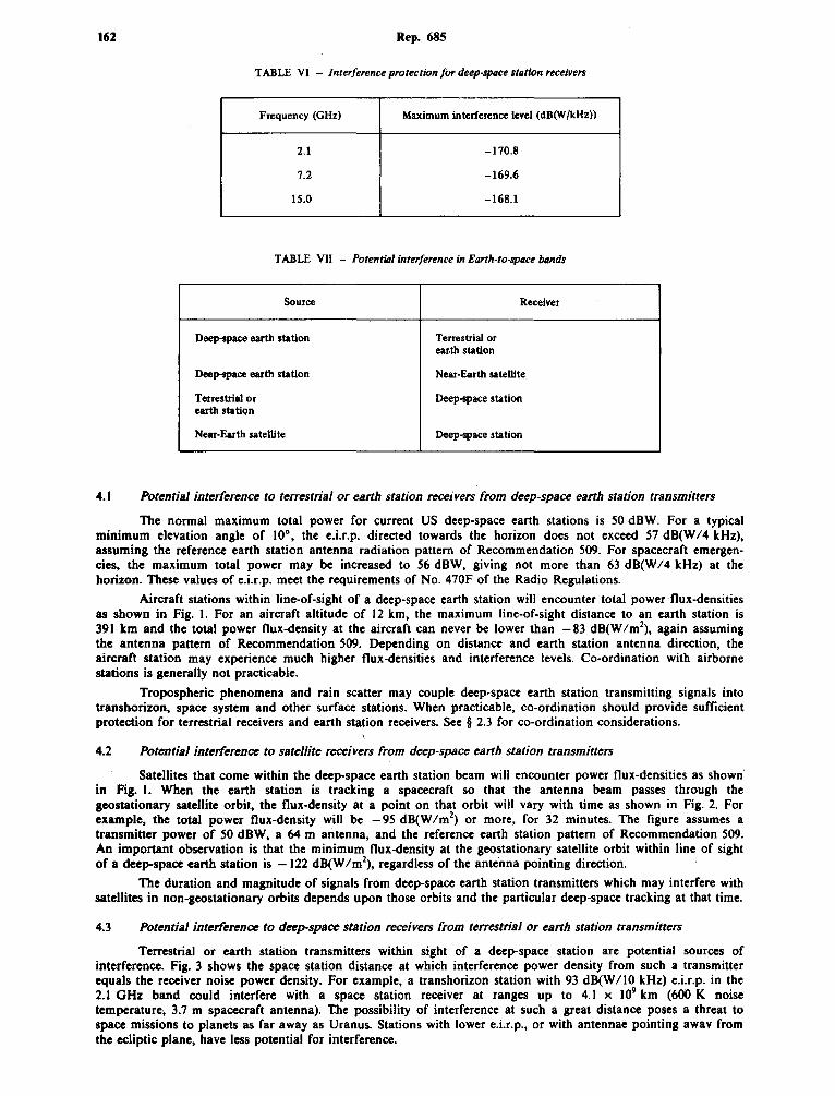
162 Rep. 685

TABLE VI - Interference protection for deep·qHlCe ltation receivers

Frequency (GHz) Maximum interference level (dB(W{kHz))

2.1 -170.8

7.2 -169.6

15.0 -168.1

TABLE VII - Potential interference in Earth-to-!{[Jace bands

Source Receiver

Deep-space earth station Terrestrial or ear.th station

Deep-space earth station Near-Earth satellite

Terrestrial or Deep-space station earth station

Near-Earth satellite Deep-space station

4.1 Potential interference to terrestrial or earth station receivers from deep-space earth station transmitters

The normal maximum total power for current US deep-space earth stations is 50 dBW. For a typical minimum elevation angle of 10°, the e.i.r.p. directed towards the horizon does not exceed 57 dB(W/4 kHz), assuming the reference earth station antenna radiation pattern of Recommendation 509. For spacecraft emergen­cies, the maximum total power may be increased to 56 dBW, giving not more than 63 dB(W/4 kHz) at the horizon. These values of e.i.r.p. meet the requirements of No. 470F of the Radio Regulations.

Aircraft stations within line-of-sight of a deep-space earth station will encounter total power flux-densities as shown in Fig. 1. For an aircraft altitude of 12 km, the maximum line-of-sight distance to an earth station is 391 km and the total power flux-density at the aircraft can never be lower than -83 dB(W/m2

), again assuming the antenna pattern of Recommendation 509. Depending on distance and earth station antenna direction, the aircraft station may experience much higher flux-densities and interference levels. Co-ordination with airborne stations is generally not practicable.

Tropospheric phenomena and rain scatter may couple deep-space earth station transmitting signals into transhorizon, space system and other surface stations. When practicable, co-ordination should provide sufficient protection for terrestrial receivers and earth station receivers. See § 2.3 for co-ordination considerations.

4.2 Potential interference to satellite receivers from deep-space earth station transmitters

Satellites that come within the deep-space earth station beam will encounter power flux-densities as shown· in Fig. I. When the earth station is tracking a spacecraft so that the antenna beam passes through the geostationary satellite orbit, the flux-density at a point on that orbit will vary with time as shown in Fig. 2. For example,' the total power flux-density will be -95 dB(W/m2

) or more, for 32 minutes. The figure assumes a transmitter power of 50 dBW, a 64 m antenna, and the reference earth station pattern of Recommendation 509. An important observation is that the minimum flux-density at the geostationary satellite orbit within line of sight of a deep-space earth station is - 122 dB(W I m2

), regardless of the antenna pointing direction. ·

The duration and magnitude of signals from deep-space earth station transmitters which may interfere with satellites in non-geostationary orbits depends upon those orbits and the particular deep-space tracking at that time.

4.3 Potential interference to deep-space station receivers from terrestrial or earth station transmitters

Terrestrial or earth station transmitters within sight of a deep-space station are potential sources of interference. Fig. 3 shows the space station distance at which interference power density from such a transmitter equals the receiver noise power density. For example, a transhorizon station with 93 dB(W/IO kHz) e.i.r.p. in the 2.1 GHz band could interfere with a space station receiver at ranges up to 4.1 x I09 km (600 K noise temperature, 3.7 m spacecraft antenna). The possibility of interference at such a great distance poses a threat to space missions to planets as far away as Uranus. Stations with lower e.i.r.p., or with antennae pointing awav from the ecliptic plane, have less potential for interference.

i ~

j i!

Rep. 685

107

5 I L

I I I

2 I I I

I I I

106 I f I

5 ,. I

I I I

2 I I I

I I I I

105 A/ a 1q DJ

5 I

I I ... - ·~· --r- - - -, ·--· T"

2 I I I I I I I

104 I I I I

s I . ,. I I I I

2 I I I I I I I

103 I I I I

5 . 1' .

I I I

2 I I I I ' I I I

•20 ·40 ·60 ·80 •100 ·120 ·148

Power flux-density (dB(W /m'))

FIGURE 1 - Power flux-density from earth station traMmittu JOO kW, 64 m antenna

A: Main beam, 15 GHz

B: Main beam, 2.1 GHz

C: 5° off axis (14.5 dB gain, Recommendation 509)

D: >48° off axis (-10 dB gain, Rec. 509)

___ :Altitude of geostationary satellite orbit, 3.56 X 10• km

•40

-110 0

\ \

'

""' --........ r--r--- --- -10 20 30 40 50 10 70

Cumulative time at or above minimum power flux-density (minutes)

IO

FIGURE 2 - Duration of potentilll lntuference to geostationary Jlltellite intersecting beam axis from earth station with JOO kW

tr11111mitter and 64 m antenM

-:2.lGHz

----: lSGHz

163

164

~ 8 ! ,IQ .., s:: .g ~ ., ~ Q,

"'

Rep. 685

1010

,, /

v / /

109 / /

I I ,, I ,, ,,

/ / /

0/ C/ BV A~

-7- -- ~-- - -- -/ -/ ~/-2 d

108

I I I , ,, ,, 5 / / /

" / ~

/ / /

107 / / /

I I I , , I

/ / /

/ v ~ / / /

/ / /

I I , , / /

v ~

/

105 / 0 10 20 30 40 50 60 70

Space station antenna gain (dBi)

FIGURE 3 - Space station distance from terrestrial transmitter for interference power equal to receiver noise power

A: lS GHz relay transmitter, SS dB(W/10 kHz); -168 dB(W/kHz) receiver noise power

B: 7.2 GHz relay transmitter, 55 dB(W/10 kHz); -170 dB(W/kHz) receiver noise power

C: 2.1 GHz relay transmitter, 55 dB(W /I 0 kHz); - I 71 dB(W /k.Hz) receiver noise power

D: 2.1 GHz transhorizon transmitter, 93 dB(W/10 kHz); -171 dB(W/kHz) receiver noise power

d: Space station range of I astronomical unit, l .S x I 01 km

4.4 Potential interference to deep-space station receivers from near-Earth satellite transmitters

Near-Earth satellites typically have antennae directed to the Earth or to other satellites. Interference with deep-space station receivers may occur for those brief periods when the satellite antenna is directed near the ecliptic plane. As received at deep-space stations, signals from satellites will usually be relatively weaker than those from earth stations.

S. Sharing considerations: space-to-Earth bands

Table VIII and the following paragraphs consider the possibility of interference in the deep-space research space-to-Earth bands.

TABLE VIII - Potential interfere11ce in space.to-Earth bands

Source Receiver

Deep-space station Terrestrial or earth station

Deep-space station Near-Earth satellite

Terrestrial or Deep-space earth station earth station

Near-Earth satellite Deep-space earth station

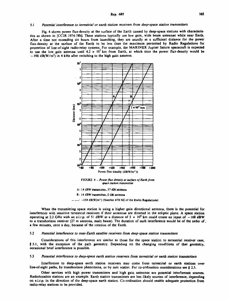
Rep. 685 165

5.1 Potential interference to terrestrial or earth station receivers from deep-space station transmitters

Fig. 4 shows power nux-density at the surface of the Earth caused by deep-space stations with characteris­tics as shown in [CCIR 1974-78b]. These stations typically use low gain, wide beam antennae while near Earth. After a time not exceeding six hours from launching, they are usually at a sufficient distance for the power flux-density at the surface of the Earth to be less than the maximum permitted by Radio Regulations for protection of line-of-sight radio-relay systems. For example, the MARINER Jupiter Saturn spacecraft is expected to use the low gain antenna until 4.2 x 107 km from Earth, at which time the power nux-density would be -198 dB(W/m2

) in 4 kHz after switching to the high gain antenna.

107

5

5

5

2

. . I

I I ,

I

I

I I

I

. . I

I I ,

' . . I

I

'

I / I I

I I I ,

' I I

I I

A/ BI I 'I ,

' 7X104 km_ . I

I i I

J I

/ I I

I !

i

I

I I

! 1o2 -80 -80 -100 •120 -MO -180 •180 -zoo

Power flux density (dB(W/m 2 ))

FIGURE 4 - Power flwc density at 1AUfoce of Earth from spoct station transmitter

A : 14 dBW tl'&llsmitter, 3 7 dBi antenna

B: 14 dBW tl'&llsmitter, 0 dBi antenna

- --= -154 dB(W/m') (Number 470 NE of the RadiQ Regulations)

When the transmitting space station is using a higher gain directional antenna, there is the potential for interference with sensitive terrestrial receivers if their antennae are directed in the ecliptic plane. A space station operating at 2.3 GHz with an e.i.r.p. of 51 dBW at a distance of 5 x 108 km could create an input of -168 dBW to a transhorizon receiver (27 m antenna, main beam). The duration of such interference would be of the order of. a few minutes, once a day, because of the rotation of the Earth.

5.2 Potential interference to near-Earth satellite receivers from deep-space station transmitters

Considerations of this interference are similar to those for the space ·station to terrestrial receiver case, f 5.1, with the exception of the path geometry. Depending on the changing conditions of that geometry, occasional brief interference is possible.

5.3 Potential interference to deep-space earth station receivers from terrestrial or earth station transmitters

Interference to deep-space earth station receivers may come from terrestrial or earth stations over line-of-sight paths, by transhorizon phenomena, or by rain scatter. For co-ordination considerations see § 2.3.

Other services with high power transmitters and high gain antennae arc potential interferen~ sources. Radiolocation stations are an example. Earth station transmitters are less likely sources of interference, depending on e.i.r.p. in the direction of the deep-space earth station.· Co-ordination should enable adequate protection from radio-relay stations to be provided.

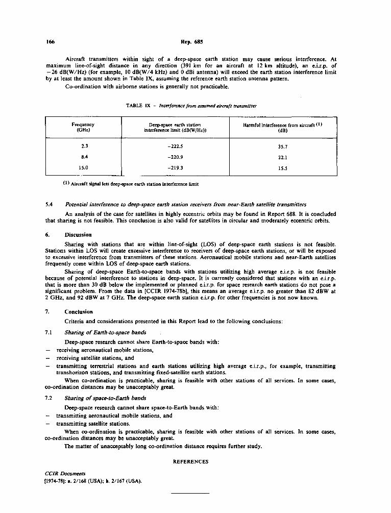
166 Rep. 685

Aircraft transmitters within sight of a deep-space earth station may cause serious interference. At maximum line-of-sight distance in any direction (391 km for an aircraft at 12 km altitude), an e.i.r.p. of -26 dB(W/Hz) (for example, 10 dB(W/4 kHz) and 0 dBi antenna) will exceed the earth station interference limit by at least the amount shown in Table IX, assuming the reference earth station antenna pattern.

Co-ordination with airborne stations is generally not practicable.

TABLE IX - Interference from asmmed aircraft transmitter

Frequency Deep-space earth station Harmful interference from aircraft (1) (GHz) interference limit (dB(W /Hz)) (dB)

2.3 -222.5 35.7

8.4 -220.9 22.1

IS.0 -219.3 15.5

(I) Aircraft signal less deep11Jace earth station interference limit

5.4 Potential interference to deep-space earth station receivers from near-Earth satel/ite transmitters

An analysis of the case for satellites in highly eccentric orbits may be found in Report 688. It is concluded that sharing is not feasible. This conclusion is also valid for satellites in circular and moderately eccentric orbits.

6. Discussion

Sharing with stations that are within line-of-sight (LOS) of deep-space earth stations is not feasible. Stations within LOS will create excessive interference to receivers of deep-space earth stations, or will be exposed to excessive interference from transmitters of these stations. Aeronautical mobile stations and near-Earth satellites frequently come within LOS of deep-space earth stations.

Sharing of deep-space Earth-to-space bands with stations utilizing high average e.Lr.p. is not feasible because of potential interference to stations in deep-space. It is currently considered that stations with an e.i.r.p. that is more than 30 dB below the implemented or planned e.i.r.p. for space research earth stations do not pose a significant problem. From the data in [CCIR 1974-78b], this means an average e.i.r.p. no greater than 82 dBW at 2 GHz, and 92 dBW at 7 GHz. The deep-space earth station e.i.r.p. for other frequencies is not now known.

7. Conclusion

Criteria and considerations presented in this Report lead to the following conclusions:

7.1 Sharing of Earth-to-space bands

Deep-space research cannot share Earth-to-space bands with: receiving aeronautical mobile stations, receiving satellite stations, and transmitting terrestrial stations and earth stations utilizing high average e.i.r.p., for example, transmitting transhorizon stations, and transmitting fixed-satellite earth stations.

When co-ordination is practicable, sharing is feasible with other stations of all services. In some cases, co-ordination distances may be unacceptably great.

7.2 Sharing of space-to-Earth bands

Deep-space research cannot share space-to-Earth bands with: transmitting aeronautical mobile stations, and transmitting satellite stations.

When co-ordination is practicable, sharing is feasible with other stations of all services. In some cases, co-ordination distances may be unacceptably great.

The matter of unacceptably long co-ordination distance requires further study.

REFERENCES

CCIR Documents (1974-78): a. 2/168 (USA); b. 2/167 (USA).

APPENDIX C

EFFECT OF SOLAR POWER SATELLITE TRANSMISSIONS ON RADIO ASTRONOMICAL RESEARCH

Chairman's Note: The following paper has been submitted by its authors to the British Royal Society of London and is reprinted here by permission of the Society.* Although its analysis is based on SPS parameters which differ somewhat from those of the current Reference System, its conclusions are similar to those of the working group. It is included here as an example of international concern over· SPS effects on radio astronomy.

The working group's brief discussion of this paper noted that the assumed parametric amplifier receiver first stage represents a worst case for out-of-passband overload sensitivity. While parametric amplifiers are extremely useful and widely used, and while all likely alternatives exhibit qualitatively similar overload phenomena, it seems likely that quantitative improvements in the overload performance of low noise receivers can be expected in the next two decades.

* The present text was retyped at PNL to improve reproducibility and PNL accepts responsibility for any typographic errors.

c .1

Effect of Solar Power Satellite transmissions on radio astronomical research

by B. Anderson and Sir Bernard Lovell, F.R.S.

Nuffield Radio Astronomy Laboratories, Jodrell Bank, University of Manchester

SUMMARY

Solar power satellites (SPS) now in the research and development stage are intended to be placed in geostationary orbits where large arrays of photocells will collect solar energy which will be delivered to Earth on a frequency of 2.45 GHz at a power level of 10 gigawatts. The calculations in this paper indicate that severe restrictions will be placed on the use of radio tele­scopes on Earth for the study of radio emissions from celestial objects. For a single SPS it would be possible to operate with the radio receiver protected by suitable filters at radio frequencies well separated from 2.45 GHz and at angles of look well displaced from the SPS. However, operational systems involving many SPS to supply significant amounts of power to Earth would create serious hazards to radio astronomical research, except possibly in thinly populated areas of the Earth.

1. Introduction It is now several years since Glaser(!) of the Arthur D. Little Consul­

tancy in the U.S. proposed that solar power should be collected by an orbit­ing satellite and beamed to Earth using a microwave transmitter. The concept is based on the consideration that the solar energy flux incident on the atmosphere (1360 W m- 2) is several times greater than mean ground level values in Europe and twice the mean flux in the Sahara. Further, at a frequency of 2.45 GHz, radiation penetrates the atmosphere from space with near unit trans­mission coefficient under all atmospheric conditions. Therefore if power is transmitted to Earth from space at this frequency there is negligible energy exchange with the atmosphere and a secure 24 hour system can be envisaged

1

with the efficiency dependent only on the conversion factors for the solar collector and transmitter in space and the collector on Earth. Substantial encouragement has now been given for the initiation of R & D on the system( 2) and in this paper we draw attention to the effects which an operational system might have on important areas of astronomical research.

2. The present proposals for a Solar Power Satellite System (SPS) In a 1975 presentation to NASA of advanced space concepts for the epoch

1980-2000 AD, Bekey( 3) outlined parameters for a system around which most of the subsequent discussion has centred. The scheme invisages a number of satel­lites in synchronous equatorial orbits. Each satellite would have solar col­lecting arrays with dimensions of 13.5 x 4.8 km feeding a 10 GW transmitter beamed to Earth on a frequency of 2.45 GHz through a 1 km aerial array. The beam would be directed to an antenna on Earth covering 10 km x 10 km and it is computed that each system would ultimately deliver 5 to 10 GW into the terrestrial distribution system. Each satellite would weigh over 11 million kg and require 20 billion photocells, and at the turn of the century it has been estimated that 8 satellites of this type could supply the UK electrical needs and that 100 could provide one-third of the U.S. electricity requirements. The power density at Earth in the 10 GW, 2.45 GHz beam transmitted from each satellite is computed to be 200 W m- 2 and we first compare this flux with that received from celestial sources by radio telescopes.

3. Interference with radio telescopes Terrestrial radio telescopes normally operate over the radio wavebands

from a few centimetres to several metres. Research in the millimetre waveband generally demands special high altitude sites and at the long wave end the ionosphere becomes the limiting factor. By normal standards the signals re­ceived from the galaxy and extragalactic objects are extremely weak. The achievable sensitivity varies over the waveband but as a guide for present purposes it may be assumed that most radio astronomical systems today work at sensitivity limits of a few millijansky (1 mJy = 10-29 W m- 2 Hz- 1). Inter­nationally regulated bands for terrestrial transmitters screen a few frequen­cies for use in radio astronomy within bandwidths of the order 4 MHz. Thus the incident flux on the antennae at limiting sensitivity is of the order

2

10-23 W m- 2. Since the flux from the SPS is of the order 1025 times that of the natural radio signals from astronomical objects it is necessary to enquire whether the operational conditions of the SPS and of radio telescopes lead to any measure of compatibility.

4. Operational circumstances The feasibility of operating radio telescopes when the 2.45 GHz beams are

incident on Earth depends (a) on the polar diagram and the sidelobe level of the solar power beamt (b) on the polar diagram and the sidelobe level of the radio telescope and (c) on the undesired ambient power levels at which the receiver of the telescope can operate. On these points the following informa­tion is available.

(a) The polar diagram of the 2.45 GHz array The 1 km diameter SPS array on 2.45 GHz will have a beam width of approx­imately 0.02 deg. The flux in the main beam collected by a 10 km "rec­tenna" on Earth will be 200 W m-2. At the edge of the rectenna the polar diagram of the SPS must be such that the radiation safety standards must be met. These allowable limits at present extend from 100 W m-2 in the USA to 0.1 W m- 2 in the USSR. We assume an intermediate value of 1 W m-2

at the edge of the collector and that by skilful design and control of the array elements in space the far-out sidelobes could be reduced to -50dB with respect to the main beam. At a level of 200 W m- 2 in the main beam the intensity of the far-out sidelobes would then be of the order 2 x 10-3 W m- 2. Howevert Kassing and Reinhertz( 4) quote a figure 50 times

· greater of 0.1 W m- 2 as the achievable diminution of flux from the SPS in the far out-zones. In the present calculations these values of 10-l and 2 x 10-3 W m- 2 are taken as the likely maximum and minimum values of the SPS flux in the far-out zones.

(b) The polar diagram of the terrestrial radio telescope We are concerned with the power delivered to the focus of the radio telescope from the 2.45 GHz transmissions from the SPS, notwithstanding the actual frequency on which the telescope is receiving the signals from celestial objects. The relevant characteristics of the radio

3

telescope are therefore those appropriate to the SPS frequency of 2.45 GHz. For simplicity we take the characteristics of the Mk IA radio telescope at Jodrell Bank. On 2.45 GHz these are -

Beam width to 3dB points = 5 arc min. Mean sidelobe level to 5° off axis = -30dB with respect to main beam. Sidelobe level beyond 5° = -60dB with respect to main beam. Effective area of the collector= 3 x 103 m 2.

We assume that the telescope is far enough removed (say more than 100 km) from the SPS terrestrial collector that it can be considered to be only in the far-out zone flux of the SPS. The power delivered at the focus for the maximum and minimum limits considered in 4(a) can then be calcu­lated for typical circumstances. Table 1 gives the power delivered to the focus for three values of e - the angle between the axis of the tele­scope beam and the SPS.

Table 1

Power delivered to the focus of the radio telescope at different values of e for two levels of the far-out zone field of the SPS.

SPS field (far-out zone} e 2 x 10-3 W m-2 10-l W m- 2

a) e < 0.1° 6W 300W b) 0.5° < e < 50 6 x 10-3w 3 x 10-1w c) e > 5° 6 x 10-6w 3 x io-4w

The power delivered to the focus of the telescope from a celestial source (assuming a limiting sensitivity of 10-29 W m-2 Hz-l and a typical bandwidth of 4 MHz) will be of the order 10-19 watts. Thus the power input from the SPS into the telescope focus will be from approximately

1014 to 1022 times greater than that from the celestial source which it is desired to study.

4

(c) The characteristics of typical radio frequency amplifiers in a disturbing field With such a great disparity between wanted and unwanted power levels the feasibility of operating a radio telescope even in the far-out field of the SPS depends on the level of rejection of the SPS signal which can be obtained by filtering at the 2.45 GHz frequency. It is possible to pro­vide adequate protection from out-of-band interfering signals for all the stages of a radio receiver except the first. The first stage is typically a parametric amplifier that has been optimised for minimum noise figure so that maximum sensitivity is achieved. Protection of a parametric amplifier by means of a filter results in a degradation in noise performance due to the insertion loss of the filter and the noise that it contributes. The amount of degradation increases with the amount of protection that is required and also as the unwanted frequency approaches the desired frequency.

Measurements have been made of the effect of out-of-band interfer­ence on several of the relatively narrow bandwidth (~ 1%) parametric amplifiers in regular use at Jodrell Bank. Three main effects have been observed:-

(;) gain compression for the case where the interfering frequency is within a few percent of the desired frequency.

(ii) detuning and gain peaking where the frequency separation is greater than in {i).

(iii) cross modulation i.e. the generation of an inband signal in the parametric amplifier from two out-of-band signals.

Many astronomical observations would be prejudiced by gain changes of 0.01% and/or spurious in-band components of 10-4 times the receiver noise. Interference levels of about 10-9 W at the parametric amplifier are sufficient to cause these changes if the frequencies are within a few percent of one another. Stronger interference can be tolerated if the frequency offset is greater.

5. Filtering requirements

The discussion in the preceding section indicates that the maximum

5

tolerable level of an interfering signal at a parametric amplifier varies from approximately 10-9 W for frequencies offset by less than 10% from the desired signal to approximately 10-7 W for offsets greater than 50%. These data are combined with those from Table 1 to deduce the specification of a filter to give the necessary protection to the parametric amplifier. The results are shown in Table 2.

Another relevant parameter of a filter is the insertion loss at the desired frequency and the effect of this on signal to noise ratios. The best parametric amplifiers currently achieve system noise temperature of about 40K; a filter with an insertion loss of 0.2 dB at room temperature would degrade signal to noise ratios with this system by 40% and, further­more, would limit the amount of possible improvement by future developments in parametric amplifiers. It is difficult to combine high rejection and low insertion loss in a filter, especially if the fractional separation of the pass and reject bands is small.

a) b) c)

Table 2

Filter attenuations required to protect the parametric amplifier from the power levels of Table 1.

The maximum and minimum values correspond to the most pessimistic and optimistic estimates respectively of the sidelobe levels from the SPS.

Filter attenuation e frequency separation frequency separation

< 10% > 50%

e < 0.1° 100 - 117 dB 80 - 97 dB 0.5° < e < 50 70 - 87 dB 50 - 67 dB e > 5° 40 - 57 dB 20 - 37 dB

6

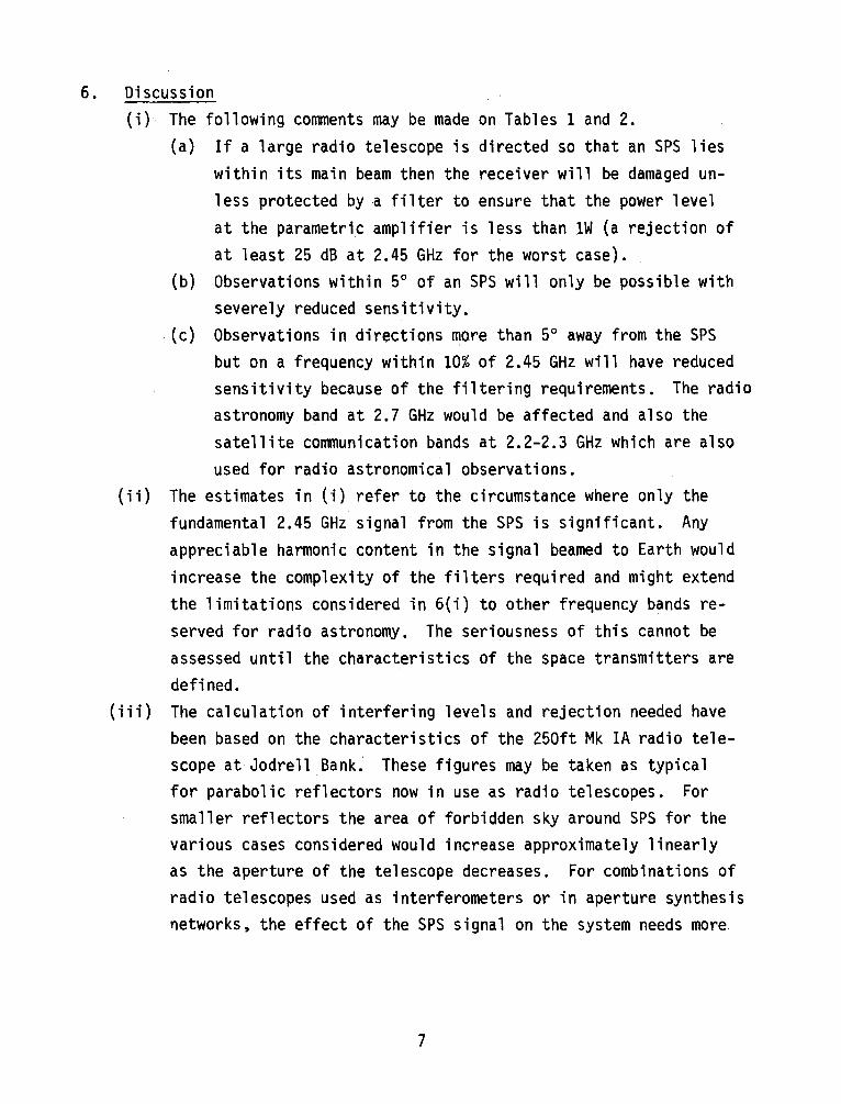
6. Discussion (i) The following comments may be made on Tables 1 and 2.

(a) If a large radio telescope is directed so that an SPS lies within its main beam then the receiver will be damaged un­less protected by a filter to ensure that the power level at the parametric amplifier is less than lW (a rejection of at least 25 dB at 2.45 GHz for the worst case).

(b) Observations within 5° of an SPS will only be possible with severely reduced sensitivity.

(c) Observations in directions more than 5° away from the SPS but on a frequency within 10% of 2.45 GHz will have reduced sensitivity because of the filtering requirements. The radio astronomy band at 2.7 GHz would be affected and also the satellite communication bands at 2.2-2.3 GHz which are also used for radio astronomical observations.

{ii) The estimates in (i) refer to the circumstance where only the fundamental 2.45 GHz signal from the SPS is significant. Any appreciable harmonic content in the signal beamed to Earth would increase the complexity of the filters required and might extend the limitations considered in 6(i) to other frequency bands re­served for radio astronomy. The seriousness of this cannot be assessed until the characteristics of the space transmitters are defined.

(iii) The calculation of interfering levels and rejection needed have been based on the characteristics of the 250ft Mk IA radio tele­scope at Jodrell BanL These figures may be taken as typical for parabolic reflectors now in use as radio telescopes. For smaller reflectors the area of forbidden sky around SPS for the various cases considered would increase approximately linearly as the aperture of the telescope decreases. For combinations of radio telescopes used as interferometers or in aperture synthesis networks, the effect of the SPS signal on the system needs more

7

detailed analysis. At best, the restrictions assessed in 6(i), as applied to the smallest aperture telescope in the network would seem to be the limiting factor.

7. Conclusions The parameters for solar power satellites now under discussion would

illuminate radio telescopes situated remotely from the SPS terrestrial col­lector at power levels at least 1020 times greater than those received from the celestial sources now being investigated and several orders of magnitude greater than those from other man made sources. The extent of the inhibition to radio astronomical research would depend critically on the polar diagram of the space array, the harmonic content of the space transmitter and the number of such power systems operating in space. For a single space station with the best attainable polar diagram and negligible harmonic radiation it should be possible to filter the interfering signal at the radio telescope so that observations would be possible except on frequencies near the protected band of 2.45 GHz, although investigations of the celestial radiation within several degrees of the satellite would be severely restricted. On the other hand,operational systems requiring several satellites to supply significant amounts of energy to Earth would create serious hazards to radio astronomical research except in thinly populated areas of the Earth. For example, it is estimated that 8 space stations would be required to supply the needs of the U.K. by 2000 AD. If the terrestrial collectors were distributed over the U.K. then it is unlikely that any site would remain for the satisfactory operation of a radio telescope.

Apart from these direct effects of the space power beam on radio astro­nomical research it may be noted that other possibilities are now under study which may influence such research. For example, measurements with the Arecibo radio telescope are in progress to determine the possible influence of the 2.45 GHz beam on the electron temperature in the ionosphere( 5); and studies at Harvard by Grossi and Colombo( 6) relate to the possibility of weather modification by using a space transmitter at 22.2 GHz. Should this be attempted then, at least,all research on the water vapour spectral line from celestial sources would be brought to a halt.

8

References and Notes

(1) P.E. Glaser - Science 162, 857, 1968.

(2) In 1978 NASA and the U.S. Department of Energy were authorised to corrmission a $25M study. Boeing Aerospace and Grurrman Corporation are involved in these studies. In the U.K., British Aerospace state that they have a £59k study contract from the European Space Agency related to this problem (British Aerospace News No.10 March 1978; Press Release 8 Feb. 1978).

(3) Bekey, I. Aerospace Corp. presentation NASA Space Station study NASA-MSFC. Dec.1975.

(4) Kassing, D. and Reinhertz, K.K. ESA Journal g_, 179, 1978. (5) Microwave Systems News, !!_, 38, 1978. (6) Grossi, M.D. and Colombo, G. Jr. of Microwave Power_!!, 209, 1977.

9

APPENDIX 0

NATIONAL ACADEMY OF SCIENCES REPORT ON SPS EFFECTS

January 23, 1979

Solar Power Satellite - Assessment of Potential for Interference to Radio Astronomy Observations

by National Academy of Sciences - National Research Council

Connnittee on Radio Frequencies

The National Aeronautics and Space Administration (NASA) and the Depart­ment of Energy (DOE) are currently exploring the feasibility of satellites placed in synchronous orbit to convert solar energy to microwaves. These micro­waves, beamed to a receiving site on the earth's surface, would be converted to 60 Hz alternating current and fed into the nation's power grid. In one con­ceptual design (NASA Publication CR-2357), each such satellite would transmit 6 gigawatts of power at a frequency near 3 GHz; eventually the system would grow to about 100 such satellites.

The power densities which would be produced in the atmosphere and on the ground by such systems are very much higher than those encountered in present­day communications and radar. This gives rise to concern about the harmful in­terference that could be caused to both terrestrial and space services. The Radio Astronomy Service is particularly sensitive to such interference, so much so that even a low-powered prototype satellite might cause serious problems at North American radio observatories.

Radio astronomy is the study of the universe by reception of natural electromagnetic waves in the wavelength range of about 1 nnn to 1 km. The radiant power detected by radio telescopes from remote cosmic sources is typi­cally 10 -lSw or less, many orders of magnitude less than the man-made signals in connnon use in the connnunications industry. Despite the low-power levels, proper frequency management, combined with the siting of radio observatories in remote rural locations, has been successful in maintaining coexistence of these two human activities.

The level of interference which can be tolerated in radio astronomy depends in a complex way on naturally occurring sources of radio noise, the kind of observation being pursued, and the bandwidth in use. The International Radio Consultative Connnittee (CCIR) Report 224-4 summarizes the results of studies of this problem (Tables 1 and 2, Appendix). The CCIR tables of harm­ful interference levels as a function of frequency have been used, for example, as guidelines in planning satellite operations that could affect radio astrornmy observations in the 2690-2700 MHz radio astronomy band.

The NASA study includes a discussion of the radio noise levels to be expected from the solar power satellite. In the initial proposal the satel­lite's transmitter would consist of 106 Arnplitron tubes. Each tube would produce about 7000 watts of power at a frequency near 2.5 GHz. Current tubes, according to the study, can achieve a noise power, in a 1 MHz band, 55 dB below the signal; with such tubes a broadband noise power of 43 dBW/MHz would be generated by the satellite in a band two hundred MHz wide centered on the signal frequency. Outside this band the noise power density would drop by 15 dB per hundred MHz.

D.l

This noise power would be focused differently from the signal. Each tube would feed one element of a phased array, each element have an effective area of about one square meter, with a forward gain of 30 dB at the design frequency, falling off slowly (1 dB/100 MHz) with frequency. !he signal beam from the 1 km diameter phased array would subtend an angle of less than an arc­minute, placing more than 90 percent of the signal in an area 10 km across the earth's surface. However, the noise voltages would not be correlated from one Amplitron to the next. Hence the noise beamwidth would be defined by the pat­tern of the individual elements, about 10°. The noise would therefore be dis­tributed over an area some thousands of miles in diameter centered on each receiving site.

The study proposes reducing this noise level, which is unacceptable even for commercial communications services, by further development of the Amplitron tubes and by filtering the signal from the tubes before it reaches the antenna elements. The filtering requirements are severe if permanent damage to radio and radar astronomy is to be avoided. The unfiltered noise signal with current tube designs would be -153 dBW m2 Hz-1 at the earth's surface. The harmful interference levels defined in the CCIR report lies some 80 to 90 dB below this level in the 2-3 GHz region. Even if adequate filters could be designed, the failure of a single one of the 106 filters could produce a noise level in excess of the harmful limits of CCIR 224-4. (These limits apply when the radio telescope is pointed away from the satellite; in a small area around the satel­lite's position the interference would be much worse). There are several other mechanisms by which serious out-of·-band interference might be generated by virtue of extremely high r-f power levels. These include non-linear effects in the earth's atmosphere and in metallic structures in the satellite or on the earth's surface.

In addition to the problems from the noise power, the signal power itself will be so high that there could be substantial interference due to the energy which goes into directions other than the main beam, and to frequencies outside the intended band. It is never possible to confine all the energy of a radio signal to the main beam and the assigned frequency'band, but with normal trans­mitters the out-of-beam and out-of-band levels are usually low enough to be negligible. The situation would be quite different for the very powerful trans­mitters being considered here, especially for interference to the very sensitive receivers used in radio astronomy.

Many observatories could be affected by any of the types of interference considered above; major U.S. installations are currently located at Green Bank, WV; Socorro, NM; Tucson, AZ; Hat Creek and OWens Vally,(sic) CA; Marfa, TX; Arecibo, PR; Amherst and Westford, MA, and Danville, IL. A remote location provides no protection from satellite interference. National borders are equally ineffective; Canadian installations in Algonquin Park, Ontario, and Penticton, BC, would also be affected. A particularly severe problem would exist for the world's most powerful and sensitive radar system, located at Arecibo, as its assigned operating frequency of 2380 MHz lies just outside the 2400-2500 MHz band currently under consideration for use by the power satellite.

D.2

Deep space communications frequencies at 2300 MHz and a radio astronomy band at 2700 MHz are other frequencies where there would be great danger of satellite-generated interference. The radio astronomy band at 5 GHz would be endangered by the second harmonic of the satellite power signal.

The Committee on Radio Frequencies concludes that the potential for harmful interference to radio astronomy is so great that protection from satellite-generated radio interference must be a major design consideration even for the earliest low-powered prototypes of the power satellite system. There may well be other radio services that share these concerns. The proposers of a new program such as this must perform adequate and realistic analyses and that work must be independently confirmed to assure that the public interest is served.

D.3

APPENDIX E

ENVIRONMENTAL CONSIDERATIONS FOR THE MICROWAVE BEAM FROM A SOLAR POWER SATELLITE

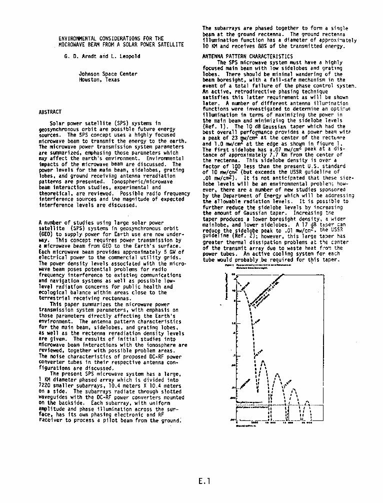
ENVIRONMENTAL CONSIDERATIONS FOR THE MICROWAVE BEAM FROM A SOLAR POWER SATELLITE

ABSTRACT

G. D. Arndt and L. Leopold

Johnson Space Center Houston, Texas

Solar power satellite (SPS) systems in geosynchronous orbit are possible future energy sources. The SPS concept uses a highly focused microwave beam to transmit the energy to the earth. The microwave power transmission system para~eters are summarized, emphasing those parameters which may affect the earth's environment. Environmental impacts of the microwave beam are discussed. The power levels for the main beam, sidelobes, grating lobes, and ground receiving antenna reradiation pattef'ns are presented. Ionospheric/microwave beam interaction studies. experimental and theoretical, are reviewed. Possible radio frequency interference sources and tne magnitude of expected interference levels are discussed.

A number of studies using large solar power satellite (SPS) systems in geosynchronous orbit (GEO) to supply power for Earth use are now under· way. This concept requires power transmission by a microwave beam from GEO to the Earth's surface. Each microwave beam provides approximately 5 GW of electrical power to the commercial utility grids. The power density levels associated with the micro· wave beam poses potential problems for radio frequency interference to existing communications and navigation systems as well as possible low­level radiation concerns for public health and ecological balance within areas close to the terrestrial receiving rectennas.

Thfs paper sunrnarizes the microwave power transmission system parameters, with emphasis on those parameters directly affecting the Earth's environment. The antenna pattern characteristics for the main beam, sidelobes, and grating lobes, as well as the rectenna reradiation density levels are given. The results of initial studies into microwave beam interactions with the ionosphere are reviewed, together with possible problem areas. The noise characteristics of proposed DC-RF power converter tubes in their respective antenna con­figurations are discussed.

The present SPS microwave system has a large, l KM diameter phased array which is divided into 7220 smaller subarrays, 10.4 meters X 10.4 meters on a side. The subarrays radiate through slotted waveguides with t~e DC-RF power converters mounted on the backside. Each subarray, with uniform amplitude and phase illumination across the sur­face, has its own phasing electronic and RF . raceiver to process a pilot beam from the ground.

The subarrays are phased together to form a single beam at the ground rectenna. The ground rectenna fllumination function has a diameter of approxi~ately 10 l<M and receives 88% of the transmitted energy.

ANTENNA PATTERN CHARACTERISTICS The SPS microwave system must have a highly

focused main beam ~tith low sidelobes and grating lobes. There should be minimal wandering of the beam boresfght, with a fail-safe mechanism in the event of a total failure of the phase control system. An active, retrodirective phasing technique satisfies this latter requirement as will be shown later. A number of different antenna illu~ination functions were investigated to determine an opti~uq illumination in terms of maximizing the power in the main beam and minimizing the sidelobe levels (Ref. 1). The 1 O dB Gaussian taper which had the best overall performance provides a power beaon witr. a peak of 23 ~/cmZ at the center of the recttnna and 1.0 mw/cm at the edge as shown in figure 1. The first sidelobe has a.07 mw/cm~ peak at a dis­tance of approximately 7.7 Km from the center of the rectenna. This sidelobe density is over a factor of 100 less than the present U.S. standard of 10 rrPN/cm2 (but exceeds the USSR guideli~e of .01 rrPN/cm2). It is not anticip11ted that these sice­lobe levels will be an environmental proble~; how­ever, there are a number of new studies sponsored. by the Department of Energy which will be a~dress1ng the allowable radiation levels. It is possible to further reduce the sidelobe levels by increasing the amount of Gaussian taper. Increasing the taper produces a lower boresight density, a wider mainlobe, and lower sidelobes. A 17 dB taper can reduce the sidelobe pe•k to .01 mw/c~2, the USSR guideline (Ref. 2); however, this large ta?er has greater thermal dissipation problems at t~e c~nter of the transmit array due to waste heat from the power tubes. An active cooling system for each tube would probably.be required for t~is taper. , .................. , ......................... . ....................... ,

---

E. l

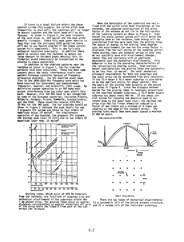
If there is a total failure within the phase control system (for example, the uplink pilot beam transmitter is shut off), the subarrays will no longer be phased together and the total beam will be de­focused. As shown in figure 1, the peak intensity of the beam drops to .003 mw/cm2 and the beam width greatly increases. Since this peak power density is less than even the stringent USSR guideline there will not be any health problem if the phase control system fails completely. This is the fail-safe mechanism mentioned previously. In addition there would be sensors near the rectenna to detect any large changes in incident power density; this in­formation would immediately be transmitted to the antenna to cease operations.

In addition to the sidelobe patterns near the rectenna as given in figure 1, the far-sidelobe patterns have been calculated. There had been some concern about the radio interference levels over eastern European countries because of frequency allocation problems. The SPS downlink power beam lies fn the 2400-2500 MHz frequency band which has been reserved for Government and nonGovernment industrial, medical, and scientific (IMS) usage. By definition anyone operating in an IMS band must accept interference from any other user within this band. However, this 100 MHz band is not recognized by some of the European countries, including Albania Bulgaria, Hungary, Poland, Ronmania, Czechoslovakia.' and the USSR. These countries reserve 2375 MHz + 50 MHz for the IMS band. The far sidelobe levels as shown in figure 2 indicate the peak levels for one 5 gigawatt SPS system are three to four orders of magnitude below .01 mw/cm2. For simultaneous operation of one hundred, ten gigawatt SPS systems the average peak level is still one to two orders ~f 11111gnitude lower than .01 mw/cm2 .

l

• ....,,,.,_,~~•••• t"•'"r Lt .... I H.lf•ai:l .. ltlAmll h11•ni.-... -•AC->tiif_..._ .... ~ .... "'

-Grating lobes, which occur at 440 Km intervals

from the rectenna, are functions of subarray size and mechanical misalinement of the subarrays within the 1 Km phased array. The grating lobes occur at spatial dfistances corresponding to angular directions off axis o the array where the signals from each of the sub-arrays add in-phase. ·

When the boresights of the subarrays are not a-1 ined with the uplink pilot beam transmitter at the rectenna, the unwanted contributions of the array factor of the antenna do not lie in the null-points of the subarray pattern as shown in figure 3. Even though.the phase control system will still point the composite beam at the rectenna, some energy will be transferred from the main beam into the grating lobes. The amount of energy in the grating lobes depends upon the misalinement (or how far the array factor is displaced from the null points of the subarray patte-· These arating lobes are somewhat unique in that they do not spatially move with misalinement changes rather they are stationary with an amplitude ' dependence upon the mechanical misalinements. This behavior is due to the operating characteristics of the retrodirective phasing syst~m. From environ­mental considerations the grating lobes are constrair::: to be less than .01 mw/cm2. The total mechanical alinement requirements for both the subarrays and the total array can be determined from this constraint. If the 10.4 meter X 10.4 meter subarray is considered to be the smallest entity for phase control, then the peaks of the grating lobe patterns at the ground are shown in figure 4. Since the distance between maxima for the grating lobes is inversely proportiona: to the spacings between subarrays, a 10.4 meter square subarray has peaks every 440 Km. If the phase con­trol system for focusing the downlink beam is ex­tended down to the power tube level, the maximum sub­array size has its linear dimension reduced by a factor of two (there are a minimum of 4 tubes per subarray at the edge of the transmit array). The grating lobes would then have peaks spaced a minimum of 880 Km apart.

.. _. --~

... '°!!!I M'tlMI

• • • • •

• • • • •

• ...........

at:CttMI \

• • ..l ... ,..

• • • • 'T

• • • • • Ptl'irte, ll'tt.l11tLt .. 11t1t•

There are two types of mechanical misalinements: 1) a systematic tilt of the entire antenna structure, and 2) a random tilt of the individual subarrays.

E.2

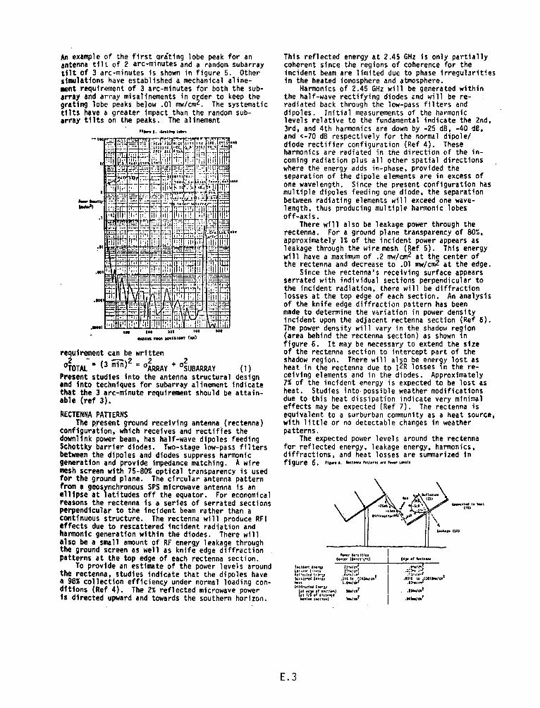
An example of the first qrating lobe peak for an antenna till of 2 arc-minutes and a random subarray tilt of 3 arc-minutes is shown in figure 5. Other simulations have established a mechanical aline­ment requirement of 3 arc-minutes for both the sub­array and array mi sa 1i nements in o~der to keep the grating lobe peaks be]ow .01 mw/cm . The systematic tilts have a greater impact than the random sub­array tilts on the peaks. The alinement

........ l.°'"lt""L~

requirement can be written 2 - -)2 2 2

0 TOTAL • (3 min ~ 0 ARRAY + 0 SUBARRAY (1) Present studies into the antenna structural design end into techniques for subarray alinement indicate thet the 3 arc-minute requirement should be attain­able (ref 3).

RECTENNA PATTERNS The Rresent ground receiving antenna (rectenna)

configuration, which receives and rectiff es the downlink power beam, has half-wave dipoles feeding Schottky barrier diodes. Two-stage low-pass filters between the dipoles and diodes suppress harmonic generation and provide impedance matching. A wire mesh screen with 75-80% optical transparency is used for the ground plane. The circular antenna pattern from a geosynchronous SPS microwave antenna is an ellipse at latitudes off the equator. For economical reasons the rectenna is a series of serrated sections perpendicular to the incident beam rather than a continuous structure. The rectenna will produce RF! effects due to rescattered incident radiation and harmonic generation within the diodes. There will also be a small amount of RF energy leakage through the ground screen as well as knife edge diffraction patterns at the top edge of each rectenna section.

To provide an estimate of the power levels around the rectenna, studies indicate that the dipoles have a 98% collection efficiency under normal loading con­ditions (Ref 4). The 2% reflected mic~owave power 1s directed upward and towards the southern horizon.

This reflected energy at 2.45 GHz is only partially coherent since the regions of coherence for the incident beam are limited due to phase irregularities in the heated ionosphere and atmosphere.

Harmonics of 2.45 GHz will be generated within the half-wave rectifying diodes end will be re­radiated back through the low-pass filters and dipoles. Initial measurements of the harmonic levels relative to the fundamental indicate the 2nd, 3rd, and 4th harmonics are down by -25 dB, -40 dB, and ~-70 dB respectively for the normal dipole/ diode rectifier configuration (Ref 4). These harmonics are radiated in the direction of the in­coming radiation plus all other spatial directions where the energy adds in-phase, provided the separation of the dipole elements are in excess of one wavelength. Since the present configuration has multiple dipoles feeding one diode, the separation between radiating elements will exceed one wave­length, thus producing multiple harmonic lobes off-axis.

There will also be leakage power through the rectenna. For a ground plane transparency of 80~. approximately 1% of the incident power appears as leakage through the wire mesh (Ref 5). This energy will have a maximum of .2 rrrH/cm2 at the center of the rectenna and decrease to .01 mw/cm2 at the edge.

Since the rectenna's receiving surface appears serrated with individual sections perpendicular to the incident radiation, there will be diffraction losses at the top edge of each section. An analysis of the knife edge diffraction pattern has been made to determine the v~riation in power density incident upon the adjacent rectenna section (Ref 6). The power density will vary in the shadow region (area behind the rectenna section) as shown in figure 6. It may be necessary to extend the size of the rectenna section to intercept part of the shadow region. There will al~o be ener~y lost as heat in the rectenna due to I2R losses in the re­ceiving elements and in the diodes. Approximately 7% of the incident energy is expected to be lost as heat. Studies into· possible weather modifications due to this heat dissipation indicate very minimal effects may be expected (Ref 7). The rectenna is equivalent to a surburban community as a heat source, with little or no detectable changes in weather patterns.

The expected power levels around the rectenna for reflected energy, leakage energy, harmonics, diffractions, and heat losses are su1TJ11arized in figure 6 t f1fll't I. llH.ttlN 'Hhr111 •~II ,..,., L .. •11

lnc14.,.t (11u11 lfl Cf~f (••r-;p ttr•uted ~.,,.~.,

k.t Utl'K [flttU'

"''' 011frut'41 '"""91

1:: ~:r.s',,~:~!~:1

N"l"' H<tlo1111I

E.3

ftftr lk"llttn C4"ttr l~rn,;~tl

lhrfc-:2

:J~;~:i ·f~~~~~~'.l*irlttif

_,,,.1 1•1f•'

,,.....,:"'lz ·~~;;:;;~ -~~~::./:>01h/cto1

.l~c-1

. ..... , ....

IONOSPHERIC INTERACTIONS The microwave beam/ionospheric interactions may

be divided into two categories: resistive (ohmic} heating effects and self-focusing instabilities. The ext(!nt of the interactions depend upon the microwave beam intensity, its frequency, the altitude (D, E, or F region), and the angle between the beam and the earth's magnetic lines. At some threshold po~er density level, nonlinear inter­actions between the power beam and the ionosphere have·been predicted to occur. These nonlinear effects could possibly degrade existing HF and VHF comnunications and VLF navigation systems due to radio frequency interference and multipath degrad­tfons. There is also concern regarding the effects of the heated fonsphere on the uplink pilot beam phasing signal. In particular the introduction of phase jitter and/or differential phase delays on the pilot beam will degrade the phase control system.

Ionospheric studies to-date indicate that thermal runaway in the E-region (110 Kilometers) and nonlinear thermal self-focusing instabilities 1n the F-region (200 to 300 kilometers) will limit the maximum power density in the beam to less than 23 rrr«/cm2 (Ref 8 to 10}. However this limit of 23 mWlcm2 (which i~ t?elieved to be correct to with· in 1 factor of twoJ 1s a theoretical result for underdense heating and has not been verified by experfment;s.

In the lower ionosphere (D and E regions), thermal conduction can be neglected; the electron heating effects are controlled by a balance between local heating and heat loss (cooling} processes. The energy loss mechanisms for the D and E regions 1111.Y be surrmarized as follows:

rotational exc1 tion

loss mechanisms

vibrational excitation

the SPS power beam. The heating and cooling con­stants for the D and E regions are short, on the order of 2 to 100 milliseconds, depending upon the altitude. Thus as the heated particles flow out of the SPS beam, the temperatures return to normal very rapidly. There is little or no coupling of the heated electrons to magnetic field lines as shown in figure 8.

N2· Oz (this loss decreases with increasing temperature}

(increases as temperature

N2,,,,~

0s

2es) ~3(P) In the upper ionosphere (F region), thermal con·

duction is the main heat loss mechanism. The heat· ing phenomenon of interest in this region is t~er~ally induced self.focusing which is predicted to produce field-alined striations. As the power density of

resonant the microwave beam increases there will be a slight transfer to focusing and defocusing of the wave due to small vibrational modes variations in the index of refraction of the

$ ~ ionospheric medium. The electric field intensity

CO H 0 increases as the incident electromagnetic wave re-fracts into regions of lesser density. Ohmic heat-

optical (in rared}excitation ing tends to drive the plasma from the focused regions,

t """ . further amplifying the self-focusing instability. 4. microns 6.5 microns The plasma thus becomes structured into large-scale

A thermal runaway can occur at these altitudes field-alined striations. As the incident field when the amount of heat deposited into a region ex- intensity increases, these striations become narrower. ceeds its cooling capacity. The studies indicate Temperature increases of 200-SOQOK will appear along the electron temperature will increase from 200°~ the magnetic field lines intersected by the micro-to lOOOOK and the electron density will increase by wave beam as shown in figure 8. The heated region 1 factor of three when the SPS beam is heating the is not confined to that volume intersected by the ionosphere (Ref 8). The electron density variation power beam since the heated particles will now as a function of altitude for SPS heating is shown traverse the magnetic field lines. The temperature 1n figure 7. In the D and E regio~s the microwave contour lines are strongly dependent upon the angle, heating slows the electron/ion recombination rate and hence the degree of coupling, between the magnetic and the density increases. The corresponding changes field lines and the power beam. The conclusions in electron temperatures for a Houston, Texas latitude from the analyses are that only those rectenna sitf>s are shown in figure 8 (Ref 8). In the D and E regio~~ at lo~er l~titudes would experience nonlinear the~ral the heated volume is confined to that subtended by self-focusing heating as determined by an angle of

E.4

incidence of seven degrees or less between the microwave beam and the earth's magnetic field lines (Ref 8).

The theoretical results indicate that a micro­wave power'densi~y of 20-25 mW/cm2.is the threshold fo·r achieving thennal runaway in the D and E regions and thermal self-focusing in the F-region (with the added requirement of 70 or less as the angle between the power beam and the magnetic field lines). Experimentally, a series of test~ were conducted at the Arecibo Observatory, Puerto Rico, in June 1977. under the direction of Dr. W. Gordon of Rice University to heat the ionosphere and to look for possible communications effects. Heating frequencies of 10 MHz, 430 MHz, and 2380 MHz were used to simu­late SPS heating effects. Using the existing facilities at Arecibo the heat input levels were below the equivalent SPS levels and the heated vol­ume was smaller. For these conditions and employing a dfagnostic radar properly located to detect any field-alined striations, no thermal runaways in the D and E reg1ons nor thermal self-focusing instabilit­ies fn the F region were observed. In addition no conmunication effects were detected.

A series of tests have been proposed using higher powers to equal or exceed the equivalent SPS heating levels in order to simulate the conditions more closely of the solar power satellite. These experiments could involve conmunications and dia­nostic tests at several facilities over the next several years, with the objectives of determining the extent of the ionosphere/microwave beam inter­actions and any effects on conrnunications/navigation systems.

T~ question of phase perturbations induced up­on the uplink pilot beam by the heated ionosphere 1s also under study now. Previously, there had been evfden_ce of.scintillations produced·by a nonrial ionosphere on microwave signals between geosynchronous satellites and the ground (Ref 11). However, these scintillations usually occur at ground stations in the tropics, fn the early evening, and at the times of equinox. For the SPS pilot beam system, the region of interest fn the heated ionosphere is a 10 meter diameter spot around boresight. This 10 meter circle fs the geometrical area subtended in the ionosphere by the 1 Km transmit array at the geosynchronous satellite as shown below. The corresponding

1angle (9) subtended by the 1 ~m array

ls (9) • sfn· 1 Km/36,000 Km = .00160 which; for an ionospheric mean height of 360 Km, subtends a 10 meter diameter area. 0

I ftE:::l I I I I I I ,-

•.ooo 1111 ~, f ' I ~10•

l ~ ; 360 ltlC I ,,

1 Uplink

·r A···"? I .. I I trrtlY I I

I I I I I I I I

I I

: I Jl,OOll Ja •110:

r ·-·· I I I I

•' 360Ja ·:

I r Slllftocl Uplink 8e1to

a~tonu11*ff9

"'1tia •' •' •' i\ I I

I ' I I I \ I I I \

l \ J60 "'° I

I I I \ I I I I

~~-~ °"""11""

flt•"" t. 1-;plierlo PorturNtlons on Uplink Pilot -

The ionosphere c,1 1 nduce several types f cfe­gradat ions to the up·, nk pilot beam including differential phase d~ il}'i (which results' in bore­sight mfsalinement), random phase jitter (which must be included 1n · ·u~ RMS phase error budget of 100 for the phase crn;trol system), and amplitude variations (resultir , in AH-to-PH conversion at the receivers in the tr. '"rr.it array). In order to determine the maxim:,:, differential phase delays permissible by the 1 ir.osphere, let us first look at the downlink power ~' -''"· All the beams from the 7220 subarrays will '' l so go through a 10 meter spot in the ionosphere tu r.~ach a point source (one dipole) at the recte--:1a. For a beam displacement at the rectenna of 5.~ meters (whfch would be 1n addition to the 50 meter displacement produced by the previously discussed 2 mean phase buildup specification on the transmit antenna), the corresponding differential phase·delay, a. in. electrical degrees is S = 3600 (X/.1225 m) where X/10 meters = 50 meters/360 Km or a • 4.0So across the 10 meter area.

On the uplink beam, ff there is a corresponding· 40 differential delay through ·the 10 meter area, then a distance, 0, where D :w (36,000 Km) {50/ 360 Km°) = 5 Km. Thus the uplink boresight beam will be shifted 5 Km from the transmit array as shown in the diagram. The 10 meter spot in the ionosphere that is actually incident upon the satellite's transmit array is shifted from boresfght by . ·

t.D =B~?o~ Km1 5 Km• 50 meters fn the ionosphere. The allowa6ie differential phase delay (on both

uplink and downlink signals) through a 10 meter dia­meter area in the heated ionosphere is 4°. Pre­liminary studies indicate the actual delay may be smaller by several orders of magnitude (Ref 12).

The pilot beam/ionosphere differential delay relationships may be sunrnarized as follows: The uplink pilot signal and the downlink power beams from each of the 7220 subarrays to a single dipole element at the rectenna will intersect a 10 meter diameter area in the ionosphere. For a differential phase delay of 40 across thfs 10 meter area, the downlink beam will be shifted by 50 meters (which has been taken as the alinement requirement for each source of error). The spatial portion of up­link pilot signal that intersects the transmit · antenna will be shifted 50 meters from true bore­sight. This shift will introduce an additional 50 meter alfnement error in the retrodfrective phase control system. (The fact that the uplink pilot and downlink power beam do not transverse the same paths through the ionosphere does not pre~ent a problem. After the retrodfrective beam leaves the satellite antenna, the required areas of coherence are limited to 10 meter diameter sections fn the ionosphere. )

The ionosphere puts an additional constraint on the uplink pilot beam signal. The present pilot beam system has double-sideband, suppressed carrier modulation which is syrrmetrical about the downlink power beam frequency, fDL' as shown below:

r "",·! :~ .£ . ~ MODULATION

'oL

E.5

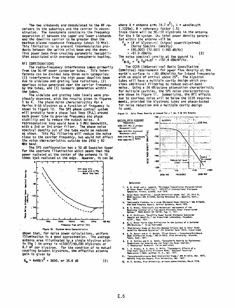
The two sidebands are-demodulated in the RF re­ceivers in the subarrays and the carrier is recon­structed. The ionosphere constrains the frequency separation ~f between the upper and lower sidebands and the downlink carrier to be greater than the maximum plasma resonance frequency (about 10 MHz). This limitation is to prevent intermodulation pro­ducts between the uplink pilot beam and the down­link power beam from creating parametric instabili­ties associated.with.overdense ionospheric heating.

RFI COt<tSIDERATIONS The radio-frequency interference comes primarily

from the DC-RF power conterter tubes. This inter­ference can be divided into three main categories: (1) interference from the high power downlink beam due to sidelobe and grating lobe radiations, (2) spurious noise generated near the carrier frequency by the tubes, and (3) harmonic generation within the tubes.

The sidelobe and grating lobe levels were pre­viously examined, with the rrsults given in figures 1 to 4. The phase noise characteristics for a Varian V-58 klystron as a function of frequency is shown in figure 10. The SPS phase control system will probably ·have a phase lock loop (PLL) around each power tube to provide frequency and phase stability and to reduce the output noise. A representative loop would have a 5 MHz bandwidth, with a 2nd or 3rd order filter. The phase noise spectral density out of the tube would be reduced as shown. This PLL filtering will reduce the noise close to the carrier frequency, but would not affect the noise characteristics outside the 2450 + 50 MHz band. -

The .SPS configuration has a lo dB Gaussian taper for the aperture illumination which means that the power radiated at the center of the antenna is 10 t1mes t~at radiated at the edge. However, it can be

1' - tube onty

-40 ---tubl w1th S l™r

j phase 10<? lo<k

] ·80 i ' \

L ' ' . ' tl ·12' ' ' !! ' . ... ... .. ... s • HO ..... j ... , ----,, s l • m

101Ufl IMl'z l~Hz 100 "11

frllqUtocy ,,.., urr11r (Kz)

'11•re 10. Kly1t"'n ll01H th1r1ctor1sttcs

shown that, for noise power calculations, uniform illumination is a good approximation. The average antenna area illuminated b¥ a single klystron with­fn th~ l Km array is n(S00)2/90,000 klystrons or 8.7 m per klystron. For the conditon of no mutual coupling between klystrons, the effective antenna gain is given by

GN • 4wAN/A2 • 3650, or 35.6 dB (2)

where A= antenna arl!a (8.7 m2), A= wavelength (.l225m), N =coherency factor (.5) Since there will oe 90, 1J'JO klystrons in the antenna for the 5 GW system, lh~ total power density genera­ted within the antenna will be

PN = (#of klystrcn~) (signal power/klystron) (Noise Spectral Density)

= (90,000) (72.000) (-160 dB/Hz) = -61. g dBW/Hz (3)

The noise spectral censity at the g~ound is PN-G a PN GN/4TIR2 ~ -187.4 dBW/m /Hz.

Th~ CCIR (Internat'onal Radio Consultative1

Committee) requirements for p~wer flux density~ at the earth's surface is -180 dBW/m /Hz for S-band frequencie: with an angle of arrival above 25°. The klystron tubes will have a multiple cavity design which pro­vides additional filtering to reduce out-of·band noise. Using a 24 dB/octave attenuation characteristic for multiple cavities, the SPS noise characteristics are shown in figure 11. Summarizing, the RFI effects due to spurious noise will be below the CCIR require­ments, provided the klystrons tubes are phase-locked for noise reduction and a multiple cavity design is used.

f19ure 11. t&o1sc Powr De-nstty at (;round for • 1 km. 5 G.W SP$ -.ntenn1

rul!.CAL AADIO A.ill,~ f.fil.U!E~.1_[_~_

1400-1417 '"" (ll1drogen luonan(t line)

ltfenincH

·Ito F----:-r- ---- . ll't'S't!!!';t~ , ~ - _- I : ·180 _ ~---,~.--CCIRJl;ti.

:::: ~~:--- ·_r;.:-~~r--t~- · _:_-::: ... •• - . .. 1 --.---- I •

·Z40 :~r-·r~~~-- 1-- ------

·ZMl I--== .... -...... --- ... --- ------. --· I ::.:-. , .'

·180 ,----------!-__;:_:__ ---~. ' lndostr1al land I ! Alo:.ron&lll!f •:IOOi_.,_ l1~1t --1 "'! ____ i •'141

.. )20 ~~ ----·---·~ --· ----~J_,_; -• __.. !1 +10 +lf)Q •1000

2450 IG1Z rREQUENCt

1. Ci. D. Arndt and L. Leopo14 1 •Mtcrownr lr"ansmtn1on Ch1r1tttrtn1c1 of Sollr Po_.r Sate111tes." 1££E>Hn-S Jntrrnu1onal Microwve 51'J1Poshr.n. Ottawa~ C'n•d1. Ju,\t 1918 .

z. So11r Power Satelltte - Syst"'1 Def1n1tton Study. Vol. tV, P•"t 'Z, NASA COntl"lct NJS 9-15196.._ 8oc1ng Uro\ptce to .• Sc•tt.le. Wash., DK. 1977.

>. •Act.tev•ble F'htreu tn • larige Mtcrwne Powr Ar'ltenn1.• RAS 9·1SC.ZJ • Mld-Ttm Pro9ren Roort. Genl!ril Dynamics. Mlirch 1978 .

4. II. C. lrown, •Electronic artd Mech•ntcal lft'IPrOv!fllt"lt of tt\e Rlocth1ng Tem1n•l of t f"ru-Spt1ct Microwave Power Trtnv.tsslon S1stem.• NASA Rcpor-t CR-1351~. A.1,19. I, 1977.

S. I. M. Dtctfoson. "Sate I 1 tte Powtir S)'Uffl'i Mic;.rowan Subs)'s.tem IMP•ct' and Benefits," Jet Propulsion l1bontory, P1Hdtn1 • C.11f,. Stpt. 1917.

6. W. C.. lrawn ·~1fe [d<Je DlffractiOl'I tn the Contut of• StrT1ttd SPS Rectenn•. • To tw: Publ tshed

7. "PN11111tnary Study of Po,.~1bh WHther Effeets due to Sohr P~dr Satellite ftectenna Opcr1t 1an'" JSC Inttrna 1 Note l 2S19. Unpubl nMd

I. L. M. l)vru;an and W. E. Gordon, "rtn•I A.t'Part • Ionospl'lere/f'Ucrow•wt lelftl lnteractlc'I Study,• NAS 9-152l2. Rict Unhustt1. Hc-uston, tu.n 1 $cpt. 1977.

t. f. V. Perktns •nd R. G. Roble, •io"osphntc He1tt"9 by A:;.dtowHes: Pritdjcttans for J.rf'c:tbtJ 1nd tht Satellite- Power Station." J. C.aaprtystc.al lluHrc"· (To b• publtshe.-$}

to. L. H. Hrilway. A. H. Katy, G. HtlU, 11 Joncspl'te-rtc £ff•cl1 of 1 Hi9h Pt1wPr SplCt-·Bllrne M1c:to1111v• 8u11," Raytt'l .. on TC"chnical Mwir.oraodU'll 1-)028, W•ltham, M.A .• Mov. 1917.

11. •ionosphere/Hlcro.,.,•ve Beari~ Jntf'r•C.t1on Stud1.· llAS •-1521Z. Deoc. 1'71,, Monthly Progren Report, Rice Univer-slty, Dec. 197'.

\2. w. [. Gordon, Rtte Unherslty, prtvlte co111r11.mlc1tton 1 fl'trcl'I '918.

E.6

ACKNOWLEDGMENTS

The editors wish to thank the National Academy of Sciences, and G. D. Arndt and L. Leopold of the Johnson Space Center for permission to reproduce material in Appendices D and E. Thanks are also extended to the International Radio Consultative Co1T111ittee for permission to reproduce reports in Appendices A and B. We would also like to thank R. A. Stokes who organized the workshop, and those who assisted in the preparation of this report, G. Long, L. Foley, T. Jewell and V. Tarr.

255