Embed Size (px)
Citation preview

Workshop on multilevel modeling II
Belkacem Abdous & Thierry [email protected]
Universite Laval
Bangalore: October 17-21, 2011
Abdous & Duchesne (Laval) MLM-Workshop October 17-21, 2010 1 / 297
Course Aims
Recap of two level models
• Introduction• Two-level models for binary responses• Subject-specific and population-averaged inferences
Advanced MLM topics
• Higher-level models with nested random effects• Higher-level models with crossed random effects
Abdous & Duchesne (Laval) MLM-Workshop October 17-21, 2010 2 / 297
Notes
Notes

Introduction
Multilevel Models
Also known as
random-effects models,
hierarchical models,
variance-components models,
random-coefficient models,
mixed models
Abdous & Duchesne (Laval) MLM-Workshop October 17-21, 2010 3 / 297
Introduction
What is multilevel modeling?
Statistical models designed for data with hierarchicalstructures or multistage samples.
Examples:• take a sample of districts, then sample individuals within
each district• pupils nested within schools• patients nested in hospitals,• people in neighborhoods,• employees in firms.
Longitudinal data is a classical example where multipleobservations over time are nested within units (e.g.subjects).
Abdous & Duchesne (Laval) MLM-Workshop October 17-21, 2010 4 / 297
Notes
Notes

Introduction
Multilevel modeling: Four Key Notions1
1-Modeling data with a complex structure:
A large range of structures that ML can handle routinely;e.g. houses nested in neighborhoods
2-Modeling heterogeneity:
standard regression models (averages), i.e. the generalrelationship, while ML additionally models variances; e.g.individual house prices vary from neighborhood toneighborhood
1From: http://www.cmm.bristol.ac.uk/Abdous & Duchesne (Laval) MLM-Workshop October 17-21, 2010 5 / 297
Introduction
Multilevel modeling: Four Key Notions2
3-Modeling dependent data:
potentially complex dependencies in the outcome over time,over space, over context; e.g.houses within a neighborhoodtend to have similar prices
4-Modeling contextuality: micro and macro and relations,
e.g. individual house prices depends on individual propertycharacteristics and on neighborhood characteristics
2From: http://www.cmm.bristol.ac.uk/Abdous & Duchesne (Laval) MLM-Workshop October 17-21, 2010 6 / 297
Notes
Notes
Introduction
Hierarchical structures
Abdous & Duchesne (Laval) MLM-Workshop October 17-21, 2010 7 / 297
Introduction
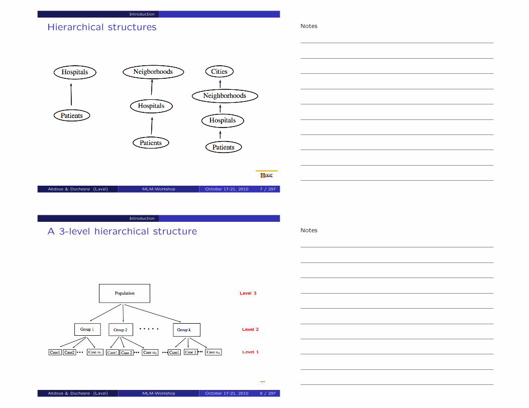
A 3-level hierarchical structure
Abdous & Duchesne (Laval) MLM-Workshop October 17-21, 2010 8 / 297
Notes
Notes

Introduction
Cross-classified structure
Abdous & Duchesne (Laval) MLM-Workshop October 17-21, 2010 9 / 297
Introduction
Cross-classified structure
Abdous & Duchesne (Laval) MLM-Workshop October 17-21, 2010 10 / 297
Notes
Notes

Introduction
Multiple membership structure
Abdous & Duchesne (Laval) MLM-Workshop October 17-21, 2010 11 / 297
Introduction
Multiple membership structure
Abdous & Duchesne (Laval) MLM-Workshop October 17-21, 2010 12 / 297
Notes
Notes

Introduction
A mix of crossed-classifications and multiplemembership structures
Abdous & Duchesne (Laval) MLM-Workshop October 17-21, 2010 13 / 297
Introduction
Analysis Strategies for Multilevel Data
Group-level analysis
Individual analysis
Contextual analysis
Analysis of covariance (fixed effects model)
Fit single-level model but adjust standard errors forclustering (GEE approach)
Multilevel (random effects) model
Abdous & Duchesne (Laval) MLM-Workshop October 17-21, 2010 14 / 297
Notes
Notes

Introduction
Group-level analysis
Aggregate to level 2 and fit standard regression models 3
Example: use the regional incidence rate of coronaryheart disease (CHD) as the dependent variable andvariables including average age and income, proportionof women etc. as independent variables.
This loses a lot of information and we riskmisinterpreting the results.
3LEYLAND AND GROENEWEGEN:http://nvl002.nivel.nl/postprint/PPpp1539.pdf
Abdous & Duchesne (Laval) MLM-Workshop October 17-21, 2010 15 / 297
Introduction
Group-level analysis
Problem : if level 2 and level 1 variables reflect differentcausal processes
Ecological or aggregation fallacy: This is the methodologicalidentification of a relationship at an area level between anoutcome and a population characteristic, and attribution ofthis relation to individuals when this relationship actuallydoes not exist at the individual level.
Abdous & Duchesne (Laval) MLM-Workshop October 17-21, 2010 16 / 297
Notes
Notes

Introduction
Group-level analysis
Robinson (1950) : correlation between illiteracy andethnicity in the USA
Level Black illiteracy Foreign-bornilliteracy
Individual 0.20 0.11(97 million people)
State( 48 units) 0.77 -0.52
Abdous & Duchesne (Laval) MLM-Workshop October 17-21, 2010 17 / 297
Introduction
Individual analysis
Use Level 1 variables and distribute level 2 characteristics tolevel 1 individuals then fit standard regression models 4
Example: assign the economic welfare of regions to allindividuals (i.e. identical for each individual within aregion).
Here we risk the atomistic fallacy : draw inferencesregarding the relation between group level variablesbased on individual level data when individual-levelassociations may differ of those at the group level.
4LEYLAND AND GROENEWEGEN:http://nvl002.nivel.nl/postprint/PPpp1539.pdf
Abdous & Duchesne (Laval) MLM-Workshop October 17-21, 2010 18 / 297
Notes
Notes

Introduction
Ecological and atomistic fallacies 5
The relationship between cost and need found amongindividuals. As need increases, so does the average cost.
The fact that individuals live in different municipalities isignored
5LEYLAND AND GROENEWEGEN:http://nvl002.nivel.nl/postprint/PPpp1539.pdf
Abdous & Duchesne (Laval) MLM-Workshop October 17-21, 2010 19 / 297
Introduction
Ecological and atomistic fallacies
The relationship between cost and need across threemunicipalities. The relationship differs little from thatfound at the individual level.
Abdous & Duchesne (Laval) MLM-Workshop October 17-21, 2010 20 / 297
Notes
Notes

Introduction
Ecological and atomistic fallacies
This ignores the data on individuals and assumes thatthe average relationships between municipalities holdbetween individuals.The relationship is fairly consistent across the threemunicipalities. An increase in need is associated with asmaller increase in cost than in the two previous figures
The average level of spending for a fixed level of needvaries between municipalities, and the ecological andindividual analyses could not take this into account.
Abdous & Duchesne (Laval) MLM-Workshop October 17-21, 2010 21 / 297
Introduction
Contextual analysis
Analyse individual-level data by including group-levelpredictors.
But : Assumes all group-level variance can be explainedby group-level predictors; incorrect SE’s for group-levelpredictors
Abdous & Duchesne (Laval) MLM-Workshop October 17-21, 2010 22 / 297
Notes
Notes

Introduction
Contextual analysis
Do pupils in single-sex school experience higher exam attainment?
Structure: 4059 pupils in 65 schools
Response: Normal score across all London pupils aged 16
Predictor: Girls and Boys School compared to Mixed school
Parameter Single level Multilevel
Cons (Mixed school) -0.098 (0.021) -0.101 (0.070)Boy school 0.122 (0.049) 0.064 (0.149)Girl school 0.245 (0.034) 0.258 (0.117)
Between school 0.155 (0.030)variance(σ2
u)Between student 0.985 (0.022) 0.848 (0.019)
variance (σ2e )
Abdous & Duchesne (Laval) MLM-Workshop October 17-21, 2010 23 / 297
Introduction
Analysis of covariance (fixed effects model)
Include dummy variables for each and every group. But
What if number of groups very large, eg households?
No single parameter assesses between group differences
Can not make inferences beyond groups in sample
Can not include group-level predictors as all degrees offreedom at the group-level have been consumed
Target of inference: individual School versus schools
Abdous & Duchesne (Laval) MLM-Workshop October 17-21, 2010 24 / 297
Notes
Notes

Introduction
GEE approach
Fit single-level model but adjust standard errors forclustering (GEE approach) But
Treats groups as a nuisance rather than of substantiveinterest;
No estimate of between-group variance;
Not extendible to more levels and complex heterogeneity
Abdous & Duchesne (Laval) MLM-Workshop October 17-21, 2010 25 / 297
Introduction
Multilevel (random effects) model
Partition residual variance into between- andwithin-group (level 2 and level 1) components.
Allows for un-observables at each level.
corrects standard errors.
Micro AND macro models analysed simultaneously.
Avoids ecological fallacy and atomistic fallacy.
Richer set of research questions BUT (as usual) needwell-specified model and assumptions met.
Abdous & Duchesne (Laval) MLM-Workshop October 17-21, 2010 26 / 297
Notes
Notes

Two-level models for binary responses
Two-level models for binary responses
Abdous & Duchesne (Laval) MLM-Workshop October 17-21, 2010 27 / 297
Two-level models for binary responses Single-level models
Logistic regression
When the distribution is binomial (e.g., binary response,such as HIV prevalence) and the link function is logit, we getthe logistic regression model:
E [yi |xi ] = P[yi = 1|xi ] = πi ;
logit(πi ) = ln(
πi1−πi
)= ln{Odds(yi = 1|xi )} = β1 +β2xi ;
Odds(yi = 1|xi ) = eβ1+β2xi ⇔ πi = eβ1+β2xi
1+eβ1+β2xi.
Abdous & Duchesne (Laval) MLM-Workshop October 17-21, 2010 28 / 297
Notes
Notes

Two-level models for binary responses Single-level models
Interpretation of the model parameters
The exponential of the model parameters are easilyinterpreted in terms of odds ratios:
eβ1: odds of getting a response of 1 when xi = 0;
eβ2: value by which odds of getting yi = 1 are multipliedwhen xi increases by 1 (and other covariates xij ’s, ifavailabe, remain unchanged).
Abdous & Duchesne (Laval) MLM-Workshop October 17-21, 2010 29 / 297
Two-level models for binary responses Single-level models
Example: Determinants of HIV prevalenceamong FSW
Ramesh et al. (AIDS 2008) use the IBBA1 data to exploreassociations between HIV prevalence and sociodemographic+ sex work characteristics of FSW in 23 districts of 4southern states.
Abdous & Duchesne (Laval) MLM-Workshop October 17-21, 2010 30 / 297
Notes
Notes

Two-level models for binary responses Single-level models
Example: Determinants of HIV prevalenceamong FSW
Model and notation:
yi = 1 if i-th FSW is HIV positive, yi = 0 otherwise
xi = (1,xi1,xi2, . . . ,xip): sociodemographic and sex workcharacteristics of i-th FSW
Model:logit(P[Yi = 1|xi ]) = β′xi = β0 +β1xi1 +β2xi2 + · · ·+βpxip
Abdous & Duchesne (Laval) MLM-Workshop October 17-21, 2010 31 / 297
Two-level models for binary responses Single-level models
Example: Determinants of HIV prevalenceamong FSW
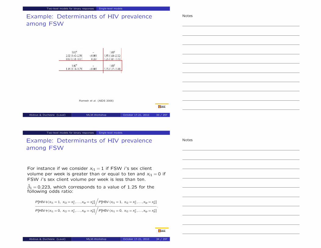
Ramesh et al. (AIDS 2008)Abdous & Duchesne (Laval) MLM-Workshop October 17-21, 2010 32 / 297
Notes
Notes
Two-level models for binary responses Single-level models
Example: Determinants of HIV prevalenceamong FSW
Ramesh et al. (AIDS 2008)
Abdous & Duchesne (Laval) MLM-Workshop October 17-21, 2010 33 / 297
Two-level models for binary responses Single-level models
Example: Determinants of HIV prevalenceamong FSW
For instance if we consider xi1 = 1 if FSW i’s sex clientvolume per week is greater than or equal to ten and xi1 = 0 ifFSW i’s sex client volume per week is less than ten.
β1 = 0.223, which corresponds to a value of 1.25 for thefollowing odds ratio:
P[HIV+|xi1 = 1, xi2 = x∗2 , . . . ,xip = x∗p ]
/P[HIV-|xi1 = 1, xi2 = x∗2 , . . . ,xip = x∗p ]
P[HIV+|xi1 = 0, xi2 = x∗2 , . . . ,xip = x∗p ]
/P[HIV-|xi1 = 0, xi2 = x∗2 , . . . ,xip = x∗p ]
.
Abdous & Duchesne (Laval) MLM-Workshop October 17-21, 2010 34 / 297
Notes
Notes

Two-level models for binary responses Two-level random intercept model
Two-level random intercept logistic model
Suppose that we have individuals (level 1) within districts(level 2). We might need to
relax the assumption of independence among individualsin a same district;
incorporate the potential effects of omitted/unobserveddistrict-specific variables in the model;
allow the odds of having a response equal to 1 for equalxi1 to vary among districts.
This can be done by adding a district-level random interceptin the logistic regression model.
Abdous & Duchesne (Laval) MLM-Workshop October 17-21, 2010 35 / 297
Two-level models for binary responses Two-level random intercept model
Two-level random intercept logistic model
Let
yij be the response for individual i in district j;
x1ij = (x1ij1,x1ij2, . . . ,x1ijp)′ be the individual level covariatesfor individual i in district j.
x2j = (x2j1,x2j2, . . . ,x2jq)′ be the district level covariates fordistrict j;
The random intercept logistic regression model assumes that
logit{P[yij = 1|xij , ζj ]} = β0 +β′1x1ij +β′2x2j + ζj ,
with ζj ∼N(0,Ψ) a district-specific random intercept.
Abdous & Duchesne (Laval) MLM-Workshop October 17-21, 2010 36 / 297
Notes
Notes
Two-level models for binary responses Two-level random intercept model
Interpretation of the random intercept logisticmodel
β0: log-odds of yij = 1 when x2j = x3ij = ζj = 0;
β1k : increase in log-odds of yij = 1 when x1ijk increases byone unit, but other x1ij`’s, ζj and x2j remain unchanged⇒effect of increasing the value of x1ijk by one unitwithout changing district and holding the value of allother covariates fixed.
β2k : increase in log-odds of yij = 1 when x2jk increases byone unit, but ζj and all other covariates remainunchanged⇒effect of increasing the value of x2jk by one unitwithout changing district and holding the value of x1ij
fixed;
Abdous & Duchesne (Laval) MLM-Workshop October 17-21, 2010 37 / 297
Two-level models for binary responses Example: HIV in FSW
Example: Determinants of HIV prevalenceamong FSW
Ramesh et al. (AIDS 2008) fitted a two-level randomintercept model with only individual level covariates:
yij = 1 if i-th FSW in j-th district is HIV positive, yij = 0otherwise
x1ij : sociodemographics and sex work characteristics fori-th FSW in j-th district
Model:logit(P[yij = 1|x1ij , ζj ]) = β0 +β11x1ij1 + · · ·+β1px1ijp + ζj , withζj ∼N(0,Ψ).
Abdous & Duchesne (Laval) MLM-Workshop October 17-21, 2010 38 / 297
Notes
Notes

Two-level models for binary responses Example: HIV in FSW
Example: Determinants of HIV prevalenceamong FSW
Ramesh et al. (AIDS 2008)
Abdous & Duchesne (Laval) MLM-Workshop October 17-21, 2010 39 / 297
Two-level models for binary responses Example: HIV in FSW
Example: Determinants of HIV prevalenceamong FSW
Ramesh et al. (AIDS 2008)
Abdous & Duchesne (Laval) MLM-Workshop October 17-21, 2010 40 / 297
Notes
Notes

Two-level models for binary responses Example: HIV in FSW
Example: Determinants of HIV prevalenceamong FSW
For instance, the estimate of the coefficient in front of thecovariate that is 1 if the FSW has more than 10 clients perweek is β = 0.107, with a standard error of 0.06. Thecorresponding odds ratio would be exp(0.107) = 1.11.
The estimate of the variance of the random intercepts isΨ = 0.347.
Abdous & Duchesne (Laval) MLM-Workshop October 17-21, 2010 41 / 297
Two-level models for binary responses Example: HIV in FSW
Determinants of HIV prevalence among FSW
Ramesh et al fitted the model using the PQL method inMLwiN. We can fit it by maximum likelihood (more on this ina few moments) using Stata’s xtmelogit:
************
* Read data in data and declare as panel data,
* define response variable hiv_prev
************
use "F:\IBBA1.dta", clear
xtset districtnum
generate hiv_prev = abs(hiv_final-2)
********
* Null model
********
xtmelogit hiv_prev || districtnum: ///
, variance intpoints(12)
Abdous & Duchesne (Laval) MLM-Workshop October 17-21, 2010 42 / 297
Notes
Notes

Two-level models for binary responses Example: HIV in FSW
Determinants of HIV prevalence among FSW
**************
* Random intercept model
**************
xtmelogit hiv_prev ib(2).CurrentAge ///
ib(1).MaritalStatus ib(2).Literacy ///
ib(1).IncomeOtherSources ib(1).PlaceSolicit ib(1).SexVolume ///
ib(1).DurationSW ib(2).SexWorkDebut ib(2).SexDebut ///
|| districtnum: , variance intpoints(12)
* RAN IN ABOUT 2 MINUTES
estimates store RameshRI1
matrix ri1 = e(b)
Abdous & Duchesne (Laval) MLM-Workshop October 17-21, 2010 43 / 297
Two-level models for binary responses Example: HIV in FSW
Example: Determinants of HIV prevalenceamong FSW
Abdous & Duchesne (Laval) MLM-Workshop October 17-21, 2010 44 / 297
Notes
Notes

Two-level models for binary responses Example: HIV in FSW
Example: Determinants of HIV prevalenceamong FSW
Abdous & Duchesne (Laval) MLM-Workshop October 17-21, 2010 45 / 297
Two-level models for binary responses Example: HIV in FSW
Example: Determinants of HIV prevalenceamong FSW
Abdous & Duchesne (Laval) MLM-Workshop October 17-21, 2010 46 / 297
Notes
Notes

Two-level models for binary responses Example: HIV in FSW
Example: Determinants of HIV prevalenceamong FSW
Abdous & Duchesne (Laval) MLM-Workshop October 17-21, 2010 47 / 297
Two-level models for binary responses Example: HIV in FSW
Example: Determinants of HIV prevalenceamong FSW
Fitting the same model with Stata’s gllamm:
gllamm hiv_prev ///
AgeLess25 WidDivSepDeva Unmarried Literate ///
NoOtherIncome Brothels PubPlaces ///
Clients10plus Duration5plus ///
StartedWorkLess20 SexDebutLess15 ///
, i(districtnum) link(logit) family(binom) nip(3)
* RAN IN 2.5 MINUTES
estimates store RameshRI3
matrix ri3 = e(b)
Abdous & Duchesne (Laval) MLM-Workshop October 17-21, 2010 48 / 297
Notes
Notes

Two-level models for binary responses Example: HIV in FSW
Example: Determinants of HIV prevalenceamong FSW
* Then use ri3 as starting value for more quadrature points
gllamm hiv_prev ///
AgeLess25 WidDivSepDeva Unmarried Literate ///
NoOtherIncome Brothels PubPlaces ///
Clients10plus Duration5plus ///
StartedWorkLess20 SexDebutLess15 ///
, i(districtnum) link(logit) family(binom) ///
from(ri3) nip(15)
* RAN IN 7 MINUTES
estimates store RameshRI15
matrix ri15 = e(b)
Abdous & Duchesne (Laval) MLM-Workshop October 17-21, 2010 49 / 297
Two-level models for binary responses Example: HIV in FSW
Example: Determinants of HIV prevalenceamong FSW
Abdous & Duchesne (Laval) MLM-Workshop October 17-21, 2010 50 / 297
Notes
Notes

Two-level models for binary responses Example: HIV in FSW
Example: Determinants of HIV prevalenceamong FSW
Abdous & Duchesne (Laval) MLM-Workshop October 17-21, 2010 51 / 297
Two-level models for binary responses Latent-response formulation
Latent-response formulation
To interpret the value of the variance estimates in randomintercept models, it is useful to rewrite the logistic regressionmodel as a latent-response model.
Suppose that y ∗i is an unobserved variable (e.g., “propensity”to contract diseases), but that we observe yi defined as
yi =
{1, if y ∗i > 00, otherwise.
,
with y ∗i = β0 +β1xi + εi .
If εi follows a standard logistic distribution (mean 0, varianceθ = π2/3≈ 3.29), we get the logistic regression model for yi .
Abdous & Duchesne (Laval) MLM-Workshop October 17-21, 2010 52 / 297
Notes
Notes

Two-level models for binary responses Latent-response formulation
Latent-response formulation
From Rabe-Hesketh & Skrondal (2005, p. 239)
Abdous & Duchesne (Laval) MLM-Workshop October 17-21, 2010 53 / 297
Two-level models for binary responses Latent-response formulation
Latent-response formulation
Now to get the two-level random intercept model, supposethat y ∗ij is an unobserved variable, but that we observe yij
defined as
yij =
{1, if y ∗ij > 00, otherwise.
,
with y ∗ij = β0 +β′1x1ij +β′2x2j + ζj + εij .
If εij is independent of ζj and follows a standard logisticdistribution, we get the random intercept logistic regressionmodel for yij .
Abdous & Duchesne (Laval) MLM-Workshop October 17-21, 2010 54 / 297
Notes
Notes

Two-level models for binary responses Latent-response formulation
Latent variable formulation
This formulation yields an interesting interpretation for Ψ:
correlation(y ∗ij ,y∗i ′j |xij ,xi ′j) =
Ψ
Ψ + 3.29= VPC .
⇒ Ψ controls the conditional within-district correlation.
Abdous & Duchesne (Laval) MLM-Workshop October 17-21, 2010 55 / 297
Two-level models for binary responses Latent-response formulation
Latent variable formulation
VPC is often referred to as the variance partition coefficient.
It is interpreted as the proportion of the residual (i.e.,unexplained by covariates) variability in the latent response(e.g., propensity to contract diseases) explained bybetween-district variations.
Abdous & Duchesne (Laval) MLM-Workshop October 17-21, 2010 56 / 297
Notes
Notes
Two-level models for binary responses Latent-response formulation
Latent variable formulation
Because θ = Var (y ∗ij |ζj) = Var (εij) = 3.29 is fixed, omitting level1 covariates x1ijk from a random-intercept logistic modelcannot result in an increase in the unexplained level 1variability Ψ.
But because VPC is increased (there is more unexplainedvariability), there will be an increase in the estimate of Ψ.
Abdous & Duchesne (Laval) MLM-Workshop October 17-21, 2010 57 / 297
Two-level models for binary responses Latent-response formulation
Example: Determinants of HIV prevalenceamong FSW
For the “Null” random intercept model in Table 4 ofRamesh et al:
Ψ = 0.514
⇒VPC = 0.514/(0.514 + 3.29)≈ 0.135
Hence in the null model, 13.5% of the latent response’svariability is explained by unobserved between-districtcharacteristics.
Abdous & Duchesne (Laval) MLM-Workshop October 17-21, 2010 58 / 297
Notes
Notes

Two-level models for binary responses Latent-response formulation
Example: Determinants of HIV prevalenceamong FSW
In the random intercept model with covariates (column 2 ofTable 4 of Ramesh et al):
Ψ = 0.347
⇒VPC = 0.347/(0.347 + 3.29)≈ 0.095
So 9.5% of the residual variability (variability in y ∗
unexplained by the individual-level covariates) is explained bybetween-district variations.
Abdous & Duchesne (Laval) MLM-Workshop October 17-21, 2010 59 / 297
Two-level models for binary responses Two-level random coefficient model
Two-level random coefficient (slope) model
It is possible to generalize the model so that the effect ofthe level 1 covariates is different in each district.
This can be done by adding random coefficients in front ofsome of the individual-level covariates of the model:
logit{P[yij = 1|x1ij ,x2j , ζ0j , ζ1j ]} = β0 + ζ0j + (β1 + ζ1j)x1ij1
+β12x1ij2 + · · ·+β1px1ijp
+β2x2j ,
where (ζ0j , ζ1j) are assumed to follow a bivariate normaldistribution with mean vector (0,0), Var (ζ0j) = Ψ00,Var (ζ1j) = Ψ11 and Cov (ζ0j , ζ1j) = Ψ01.
Abdous & Duchesne (Laval) MLM-Workshop October 17-21, 2010 60 / 297
Notes
Notes

Two-level models for binary responses Two-level random coefficient model
Two-level random coefficient (slope) model
Interpretation:
(β1 + ζ1j) is the increase in the log-odds of yij = 1 for anindividual in district j whose value of x1ij1 increases byone unit;
β1 is the same increase, but in an “average district”, i.e.a district for which ζ1j = 0;
Abdous & Duchesne (Laval) MLM-Workshop October 17-21, 2010 61 / 297
Two-level models for binary responses Two-level random coefficient model
Example: Determinants of HIV prevalenceamong FSW (cont’d)
Ramesh et al. (AIDS 2008) also fitted two-level randomcoefficient models to the IBBA1 data:
yij = 1 if i-th FSW in j-th district is HIV positive, yij = 0otherwise
x1ij : sociodemographic and sex work characteristics fori-th FSW in j-th district
Abdous & Duchesne (Laval) MLM-Workshop October 17-21, 2010 62 / 297
Notes
Notes

Two-level models for binary responses Two-level random coefficient model
Example: Determinants of HIV prevalenceamong FSW (cont’d)
The model in column 3 (random intercept and randomcoefficients in front of marital status indicators):
logit(P[yij = 1|x1ij , ζj ]) = (β0 + ζ0j)
+ (β11 + ζ1j)x1ij1 + (β12 + ζ2j)x1ij2
+β13x1ij3 + · · ·+β1px1ijp,
(ζ0j , ζ1j , ζ2j)′ ∼N
(0,0,0)′,Ψ =
Ψ0,0 Ψ0,1 Ψ0,2
Ψ0,1 Ψ1,1 Ψ1,2
Ψ0,2 Ψ1,2 Ψ2,2
x1ij1 = 1 if widowed/divorsed/separated/devadasi
x1ij2 = 1 if unmarried.
Abdous & Duchesne (Laval) MLM-Workshop October 17-21, 2010 63 / 297
Two-level models for binary responses Two-level random coefficient model
Example: Determinants of HIV prevalenceamong FSW (cont’d)
Abdous & Duchesne (Laval) MLM-Workshop October 17-21, 2010 64 / 297
Notes
Notes

Two-level models for binary responses Two-level random coefficient model
Example: Determinants of HIV prevalenceamong FSW (cont’d)
Abdous & Duchesne (Laval) MLM-Workshop October 17-21, 2010 65 / 297
Two-level models for binary responses Two-level random coefficient model
Determinants of HIV prevalence among FSW(cont’d)
Fitting the model with Stata’s xtmelogit
**************
* Random slope (marital status)
**************
* First, with Laplace approximation and a simple
* variance-covariance structure
xtmelogit hiv_prev ///
AgeLess25 WidDivSepDeva Unmarried Literate ///
NoOtherIncome Brothels PubPlaces ///
Clients10plus Duration5plus ///
StartedWorkLess20 SexDebutLess15 ///
|| districtnum: WidDivSepDeva Unmarried, ///
variance laplace
* RAN IN 5 MINUTES
matrix rs1un1 = e(b)
Abdous & Duchesne (Laval) MLM-Workshop October 17-21, 2010 66 / 297
Notes
Notes

Two-level models for binary responses Two-level random coefficient model
Determinants of HIV prevalence among FSW(cont’d)
* Same, with more complex variance-covariance structure
* and 5 quadrature points
matrix a1 = (rs1un1,0,0,0)
xtmelogit hiv_prev ///
AgeLess25 WidDivSepDeva Unmarried Literate ///
NoOtherIncome Brothels PubPlaces ///
Clients10plus Duration5plus ///
StartedWorkLess20 SexDebutLess15 ///
|| districtnum: WidDivSepDeva Unmarried, ///
variance covariance(unstructured) ///
intpoints(5) from(a1,copy) refineopts(iterate(0))
* RAN IN 18 MINUTES
Abdous & Duchesne (Laval) MLM-Workshop October 17-21, 2010 67 / 297
Two-level models for binary responses Two-level random coefficient model
Example: Determinants of HIV prevalenceamong FSW (cont’d)
Abdous & Duchesne (Laval) MLM-Workshop October 17-21, 2010 68 / 297
Notes
Notes

Two-level models for binary responses Two-level random coefficient model
Example: Determinants of HIV prevalenceamong FSW (cont’d)
Abdous & Duchesne (Laval) MLM-Workshop October 17-21, 2010 69 / 297
Two-level models for binary responses Two-level random coefficient model
Example: Determinants of HIV prevalenceamong FSW (cont’d)
To get the values in column 3 of Table 4 of Ramesh et al:
Var (ζ0j + x1ij1ζ1j + x1ij2ζ2j) = Ψ00 + x21ij1Ψ11 + x2
1ij2Ψ22
+ 2x1ij1Ψ01 + 2x1ij2Ψ02 + 2x1ij1x1ij2Ψ12.
With maximum likelihood, 5 quadrature points, xtmelogit:
Married (x1ij1 = x1ij2 = 0): 0.55 [With PQL, from Ramesh et al., Table
4: 0.62]
Widowed/Divorced/Separated/Devadasi (x1ij1 = 1, x1ij2 = 0):0.55 + 0.13 + 2∗ (−0.20) = 0.28 [With PQL, from Ramesh et al., Table
4: 0.31]
Never married (x1ij1 = 0, x1ij2 = 1):0.55 + 0.11 + 2∗ (−0.21) = 0.24 [With PQL, from Ramesh et al., Table
4: 0.27]
Abdous & Duchesne (Laval) MLM-Workshop October 17-21, 2010 70 / 297
Notes
Notes

Two-level models for binary responses Two-level random coefficient model
Example: Determinants of HIV prevalenceamong FSW (cont’d)
The effect of marital status (odds ratios of being HIV+when divorced or never married vs married) is not the samefrom one district to the other.
If we look at the xtmelogit output, we have a coefficient of0.66 with a variance of 0.28 for Widowed, etc. vs married.
⇒ log-odds ratio of being HIV+ for Widowed, etc. vsmarried varies among districts according to a N(0.66, 0.28)distribution.
Abdous & Duchesne (Laval) MLM-Workshop October 17-21, 2010 71 / 297
Two-level models for binary responses Two-level random coefficient model
Example: Determinants of HIV prevalenceamong FSW (cont’d)
Some interesting calculations can then be made. Forexample:
1st quartile of N(0.66, 0.28) is given by0.66 + z0.25
√0.28 = 0.66 + (−0.67)(0.53) = 0.30, so 25% of
districts have odds ratio for Divorced etc. vs Married lessthan exp(0.30) = 1.35
3rd quartile N(0.66, 0.28) is given by0.66 + z0.75
√0.28 = 0.66 + (0.67)(0.53) = 1.02, so 25% of
districts have odds ratio for Divorced etc. vs Married greaterthan exp(1.02) = 2.76
Abdous & Duchesne (Laval) MLM-Workshop October 17-21, 2010 72 / 297
Notes
Notes

Two-level models for binary responses Two-level random coefficient model
Determinants of HIV prevalence among FSW(cont’d)
Fitting the same model with Stata’s gllamm:
* Using random intercept model as starting point
matrix a2 = (ri15,0,0,0,0,0)
* Equations to define random coefficients
generate cons = 1
eq randomIntercept: cons
eq randomWid: WidDivSepDeva
eq randomUnmar: Unmarried
gllamm hiv_prev ///
AgeLess25 WidDivSepDeva Unmarried Literate NoOtherIncome ///
Brothels PubPlaces Clients10plus Duration5plus ///
StartedWorkLess20 SexDebutLess15 ///
, i(districtnum) nrf(3) eqs(randomIntercept randomWid randomUnmar) ///
link(logit) family(binom) from(a2) copy ip(m) nip(5)
Abdous & Duchesne (Laval) MLM-Workshop October 17-21, 2010 73 / 297
Two-level models for binary responses Two-level random coefficient model
Example: Determinants of HIV prevalenceamong FSW (cont’d)
Abdous & Duchesne (Laval) MLM-Workshop October 17-21, 2010 74 / 297
Notes
Notes

Two-level models for binary responses Two-level random coefficient model
Example: Determinants of HIV prevalenceamong FSW (cont’d)
Abdous & Duchesne (Laval) MLM-Workshop October 17-21, 2010 75 / 297
Two-level models for binary responses Inferences in two-level logistic models
Maximum likelihood estimation
Consider the general model
logit{P[yij = 1|x1ij ,x2j , ζj ]} = β0 +β′1x1ij +β′2x2j + ζ ′jzij ,
where ζj ∼N(0,Ψ) and zij is specified so as to obtain thedesired random intercept or random coefficient model.
Maximum likelihood estimation consists in finding the valuesof β = (β0,β′1,β
′2)′ and Ψ that maximize the probability of the
observed data.
Abdous & Duchesne (Laval) MLM-Workshop October 17-21, 2010 76 / 297
Notes
Notes

Two-level models for binary responses Inferences in two-level logistic models
Likelihood function
The likelihood function is the probability of the observedresponses given the observed covariates:
L(β,Ψ) = P[yij , i = 1, . . . ,nj , j = 1, . . . ,N|X]
=N∏
j=1
P[yij , i = 1, . . . ,nj |Xj ]
=N∏
j=1
∫P[yij , i = 1, . . . ,nj |Xj , ζj ]φ(ζj ;0,Ψ) dζj ,
where φ(ζj ;0,Ψ) is the density of the multivariate normaldistribution with mean vector 0 and variance matrix Ψ.
All one needs to do is find the value of β and Ψ thatmaximize L(β,Ψ), but ...
Abdous & Duchesne (Laval) MLM-Workshop October 17-21, 2010 77 / 297
Two-level models for binary responses Inferences in two-level logistic models
Numerical integration and maximization
... the integral in L(β,Ψ) cannot be evaluated in closed formfor two-level logistic models:
L(β,Ψ) =N∏
j=1
∫ ni∏i=1
eβ0+β′1x1ij +β
′2x2j +ζ
′j zij
1 + eβ0+β′1x1ij +β′
2x2j +ζ′j zij
× (2π||Ψ||)−d/2 exp
(−
1
2ζ′j Ψ−1ζj
)dζj ,
where d = dim(ζj) and ||Ψ|| is the absolute value of thedeterminant of Ψ.
⇒ Software combines numerical integration methods withnumerical maximization.
Abdous & Duchesne (Laval) MLM-Workshop October 17-21, 2010 78 / 297
Notes
Notes

Two-level models for binary responses Inferences in two-level logistic models
Stata implementation
Numerical integration in maximum likelihood is performed byxtmelogit and gllamm using quadrature methods. Thenumber of quadrature points can be specified: the higherthe number of points, the more precise the likelihoodevaluation, the better the estimates of the elements of Ψ ...but the slower the execution!
xtmelogit: Use option intpoint(#). [With #=1 we getthe Laplace approximation (good estimates of β, poorestimates of Ψ). We use Laplace to get starting pointsfor method with #≥ 3.]
gllamm: Use option nip(#). [Laplace method not allowed,so use with #≥ 3.]
Abdous & Duchesne (Laval) MLM-Workshop October 17-21, 2010 79 / 297
Two-level models for binary responses Inferences in two-level logistic models
Fitting random intercept and randomcoefficient models
In the random intercept model, d =dim(ζj) = 1, so integrationin one dimension: easy and quick, so we can use largenumber of quadrature points (say 12 or 20).
When fitting a model with random coefficients as well, thend =dim(ζj)≥ 2, so numerical integration now in higherdimension.
⇒Fitting such a model with maximum likelihood isnumerically quite challenging (much, much slower than whend = 1).
Abdous & Duchesne (Laval) MLM-Workshop October 17-21, 2010 80 / 297
Notes
Notes

Two-level models for binary responses Inferences in two-level logistic models
Getting maximum likelihood estimation toconverge
Some tricks to achieve convergence with maximumlikelihood:
Start with the Laplace method (1 quadrature point) anduse its results as starting point for quadrature with morequadrature points.
Try fitting a model with a simpler structure for Ψ (e.g.,diagonal structure, the default in xtmelogit).
If the database is not too large (unfortunately not thecase of IBBA ...), use the “data cloning” method totrick WinBUGS into giving you the maximum likelihoodestimators. (Create a new dataset that is comprised of a large number of copies of the
current dataset, then fit Bayesian model with flat priors ⇒ posterior mean is maximum likelihood
estimate and posterior variance is variance of estimate.)
Abdous & Duchesne (Laval) MLM-Workshop October 17-21, 2010 81 / 297
Two-level models for binary responses Inferences in two-level logistic models
Example: Determinants of HIV prevalenceamong FSW
Fitting the random coefficient model with Stata’s xtmelogit:
**************
* Random slope (marital status)
**************
* First, with Laplace approximation and a
* simple variance-covariance structure
xtmelogit hiv_prev ///
AgeLess25 WidDivSepDeva Unmarried Literate ///
NoOtherIncome Brothels PubPlaces ///
Clients10plus Duration5plus ///
StartedWorkLess20 SexDebutLess15 ///
|| districtnum: WidDivSepDeva Unmarried, ///
variance laplace
* RAN IN 5 MINUTES
estimates store RameshRS1UN1
matrix rs1un1 = e(b)
Abdous & Duchesne (Laval) MLM-Workshop October 17-21, 2010 82 / 297
Notes
Notes

Two-level models for binary responses Inferences in two-level logistic models
Example: Determinants of HIV prevalenceamong FSW
* Same, with more complex variance-covariance structure
* and 5 quadrature points
matrix a1 = (rs1un1,0,0,0)
xtmelogit hiv_prev ///
AgeLess25 WidDivSepDeva Unmarried Literate ///
NoOtherIncome Brothels PubPlaces ///
Clients10plus Duration5plus ///
StartedWorkLess20 SexDebutLess15 ///
|| districtnum: WidDivSepDeva Unmarried, ///
variance covariance(unstructured) ///
intpoints(5) from(a1,copy) refineopts(iterate(0))
* RAN IN 18 MINUTES
estimates store RameshRS5UN
matrix rs5un = e(b)
Abdous & Duchesne (Laval) MLM-Workshop October 17-21, 2010 83 / 297
Two-level models for binary responses Inferences in two-level logistic models
Example: Determinants of HIV prevalenceamong FSW (cont’d)
Abdous & Duchesne (Laval) MLM-Workshop October 17-21, 2010 84 / 297
Notes
Notes

Two-level models for binary responses Inferences in two-level logistic models
Example: Determinants of HIV prevalenceamong FSW (cont’d)
Abdous & Duchesne (Laval) MLM-Workshop October 17-21, 2010 85 / 297
Two-level models for binary responses Inferences in two-level logistic models
Determinants of HIV prevalence among FSW(cont’d)
Fitting the model with Stata’s gllamm
* Using random intercept model as starting point
matrix a2 = (ri15,0,0,0,0,0)
* Equations to define random coefficients
generate cons = 1
eq randomIntercept: cons
eq randomWid: WidDivSepDeva
eq randomUnmar: Unmarried
gllamm hiv_prev ///
AgeLess25 WidDivSepDeva Unmarried Literate NoOtherIncome ///
Brothels PubPlaces Clients10plus Duration5plus ///
StartedWorkLess20 SexDebutLess15 ///
, i(districtnum) nrf(3) eqs(randomIntercept randomWid randomUnmar) ///
link(logit) family(binom) from(a2) copy ip(m) nip(5)
Abdous & Duchesne (Laval) MLM-Workshop October 17-21, 2010 86 / 297
Notes
Notes

Two-level models for binary responses Inferences in two-level logistic models
Standard errors and approximate distribution
The preceding outputs showed standard errors. These arethe square roots of the diagonal elements of the negativehessian matrix of the log of the likelihood function(automatically calculated when numerical maximization isused).
If se(βk ) is the standard error of βk , then we have that βk isapproximately normally distributed with mean βk andvariance se(βk )2. This means that a (1−α)100% confidenceinterval for βk is given by βk ±z1−α/2se(βk ), and by
exp(βk ±z1−α/2se(βk
)for the corresponding odds ratio.
Abdous & Duchesne (Laval) MLM-Workshop October 17-21, 2010 87 / 297
Two-level models for binary responses Inferences in two-level logistic models
Standard errors and approximate distribution
For the Ramesh et al model with random coefficients, thelast xtmelogit output gave β11 = 0.66 with associatedstandard error 0.10.
Hence a 95% confidence interval for the odds ratio of beingHIV+ for Divorced, etc. vs Married is given byexp (0.66±1.96×0.10) = (1.59, 2.35).
Abdous & Duchesne (Laval) MLM-Workshop October 17-21, 2010 88 / 297
Notes
Notes

Two-level models for binary responses Inferences in two-level logistic models
Test of linear combinations
As a matter of fact, the entire vector of maximum likelihoodestimates β is approximately normally distributed with meanvector given by the true value of the parameters β andvariance matrix given by the inverse of the negative of thehessian of the log of the likelihood.
This approximate normality is used to construct Wald testsof hypotheses of the form H0 : linear combination of the βcoefficients= 0 vs H1 : this combination is not equal to 0.
Abdous & Duchesne (Laval) MLM-Workshop October 17-21, 2010 89 / 297
Two-level models for binary responses Inferences in two-level logistic models
Example: Determinants of HIV prevalenceamong FSW
Say we want to test that the odds ratio in the group ofUnmarried FSW who have more than 10 clients per weekand all other covariates at the reference level is the same asthe odds ratio of the FSW who solicit in brothels and haveall other covariates at the reference level, i.e.,
Unmarried + Clients10plus = Brothels
⇒ Unmarried + Clients10plus - Brothels = 0
Abdous & Duchesne (Laval) MLM-Workshop October 17-21, 2010 90 / 297
Notes
Notes

Two-level models for binary responses Inferences in two-level logistic models
Example: Determinants of HIV prevalenceamong FSW
This can be done with the lincom function after having fittedthe model with xtmelogit:
* Wald test of Unmarried + Clients10plus = Brothels
* Output in terms of the beta’s
lincom Unmarried + Clients10plus - Brothels
* Same test, but with output in terms of the odds ratio
lincom Unmarried + Clients10plus - Brothels, or
Abdous & Duchesne (Laval) MLM-Workshop October 17-21, 2010 91 / 297
Two-level models for binary responses Inferences in two-level logistic models
Example: Determinants of HIV prevalenceamong FSW
Abdous & Duchesne (Laval) MLM-Workshop October 17-21, 2010 92 / 297
Notes
Notes

Two-level models for binary responses Inferences in two-level logistic models
Example: Determinants of HIV prevalenceamong FSW
We can see that the p-value of the test is 0.465, hence nosignificant difference between the two groups.
Abdous & Duchesne (Laval) MLM-Workshop October 17-21, 2010 93 / 297
Two-level models for binary responses Inferences in two-level logistic models
Test that a second level is required
In Stata, xtmelogit automatically compares the model fittedwith an ordinary (level-1 only) logistic regression model. Aconservative p-value for the test H0 : ordinary logisticregression vs H1 : two-level model is given as the last line ofthe xtmelogit output.
In the xtmelogit output for the random coefficient model,with have a p-value of 0.0000, so very small, so we have verystrong evidence against the null model and so the randomintercept and coefficients have a highly significant variability.
Abdous & Duchesne (Laval) MLM-Workshop October 17-21, 2010 94 / 297
Notes
Notes

Two-level models for binary responses Inferences in two-level logistic models
Estimation of the ζj
Though the ζj are not model parameters, their values mightbe useful to compare districts. Because these values areunobserved, they must be estimated.
Unfortunately, when doing maximum likelihood, we integratethem out, so we cannot estimate them.
Abdous & Duchesne (Laval) MLM-Workshop October 17-21, 2010 95 / 297
Two-level models for binary responses Inferences in two-level logistic models
Empirical Bayes
Software that fits GLMM by maximum likelihood can easilyfind the mode of the posterior distribution of the randomeffects given the data, i.e., the values of ζj that maximize∏
j
φ(ζj ;0,Ψ)∏
i
P[yij |xij , ζj ],
with Ψ replaced by its maximum likelihood estimate. Theseare called the empirical Bayes (modal) predictions of therandom effects.
Abdous & Duchesne (Laval) MLM-Workshop October 17-21, 2010 96 / 297
Notes
Notes

Two-level models for binary responses Inferences in two-level logistic models
Caterpillar plots
Plotting estimates of the ζj ’s along with their respectiveconfidence intervals can give a good idea of how significantthe between district variability may be:
If all the ζj are close to zero, then the random effects arenot significant and a two-level model is not necessary.
Abdous & Duchesne (Laval) MLM-Workshop October 17-21, 2010 97 / 297
Two-level models for binary responses Inferences in two-level logistic models
Example: Determinants of HIV prevalenceamong FSW
Stata code ran after xtmelogit that produced the randomintercept model to get a caterpillar plot
* caterpillar plot
* store random intercept estimates in u0
predict u0, reffects
* store the standard error of random effect estimates in u0se
predict u0se, reses
* u0 and u0se repeated for each FSW, we only need one per district
egen pickone = tag(districtnum)
sort u0
generate u0rank = sum(pickone)
serrbar u0 u0se u0rank if pickone==1, scale(1.96) yline(0)
Abdous & Duchesne (Laval) MLM-Workshop October 17-21, 2010 98 / 297
Notes
Notes

Two-level models for binary responses Inferences in two-level logistic models
Example: Determinants of HIV prevalenceamong FSW
Abdous & Duchesne (Laval) MLM-Workshop October 17-21, 2010 99 / 297
Two-level models for binary responses Adding level-two explanatory variables
Random intercept vs level-two explanatoryvariables
The variability of the random intercepts in a randomintercept model can be viewed as between-district variabilityin the latent response that is due to unmodelled differencesbetween districts.
Abdous & Duchesne (Laval) MLM-Workshop October 17-21, 2010 100 / 297
Notes
Notes

Two-level models for binary responses Adding level-two explanatory variables
Random intercept vs level-two explanatoryvariables
Adding significant district-level explanatory variables in thelinear predictor should explain some of this variability andtherefore diminish the level of unexplained between-districtvariability.
Thus to explain the between-district variability, we can use alinear predictor of the form
logit{P[yij = 1|x1ij ,x2j , ζ0j ]} = β0 + ζ0j +β1x1ij
+β2x2j .
Abdous & Duchesne (Laval) MLM-Workshop October 17-21, 2010 101 / 297
Two-level models for binary responses Adding level-two explanatory variables
Example: Adding district-level variables inRamesh et al.’s study
We repeated the analysis with the random intercept modelof Table 4 of Ramesh et al, but we added district-levelvariables to the model.
Several variables were significant when added alone, but fewremained significant when added together with otherdistrict-level variables.
In the end (e.g., reverse causality, outliers, etc.), we endedup just adding the the total proportion of female (ages 15 to45) in the population, PropFem.
Abdous & Duchesne (Laval) MLM-Workshop October 17-21, 2010 102 / 297
Notes
Notes

Two-level models for binary responses Adding level-two explanatory variables
Example: Adding district-level variables inRamesh et al.’s study
Random intercept model of Table 4, but with district-levelvariable PropFem added.
rename prop_fem_pop_15_49_t PropFem
* Random intercept model with MeanAgeMar added
* Start with Laplace approximation
xtmelogit hiv_prev ///
AgeLess25 WidDivSepDeva Unmarried Literate ///
NoOtherIncome Brothels PubPlaces ///
Clients10plus Duration5plus ///
StartedWorkLess20 SexDebutLess15 ///
PropFem || districtnum: ///
, variance laplace
* MeanAgeMar || districtnum: ///
* RAN IN 1 MINUTE
matrix riAge1 = e(b)
Abdous & Duchesne (Laval) MLM-Workshop October 17-21, 2010 103 / 297
Two-level models for binary responses Adding level-two explanatory variables
Example: Adding district-level variables inRamesh et al.’s study
* Now with 12 integration points
xtmelogit hiv_prev ///
AgeLess25 WidDivSepDeva Unmarried Literate ///
NoOtherIncome Brothels PubPlaces ///
Clients10plus Duration5plus ///
StartedWorkLess20 SexDebutLess15 ///
PropFem || districtnum: ///
, variance from(riAge1,copy) ///
refineopts(iterate(0)) intpoints(12)
* MeanAgeMar || districtnum: ///
* RAN IN 2 MINUTES
estimates store RameshRIage12
matrix riAge12 = e(b)
Abdous & Duchesne (Laval) MLM-Workshop October 17-21, 2010 104 / 297
Notes
Notes

Two-level models for binary responses Adding level-two explanatory variables
Example: Adding district-level variables inRamesh et al.’s study
Abdous & Duchesne (Laval) MLM-Workshop October 17-21, 2010 105 / 297
Two-level models for binary responses Adding level-two explanatory variables
Example: Adding district-level variables inRamesh et al.’s study
Abdous & Duchesne (Laval) MLM-Workshop October 17-21, 2010 106 / 297
Notes
Notes

Two-level models for binary responses Adding level-two explanatory variables
Example: Adding district-level variables inRamesh et al.’s study
There is a negative coefficient in front of the variable ⇒decrease in district’s proportion of female is associatedwith increase in HIV prevalence.This effect is highly significant (p-value = 0.010)Variance of random intercepts went down from 0.34 to0.25 (see also caterpillar plot of random interceptestimates on next page).VPC = 0.25/(0.25 + 3.29) = 7.1%⇒ Instead of 9.5% ofthe variability in y ∗ due to unexplained between-districtvariability, we are down to 7.1%.Nonetheless, there is still a significant amount ofunexplained between-district variability (p-value oflikelihood ratio test of 0.0000), so the random interceptsare still required.
Abdous & Duchesne (Laval) MLM-Workshop October 17-21, 2010 107 / 297
Two-level models for binary responses Adding level-two explanatory variables
Example: Adding district-level variables inRamesh et al.’s study
Ramesh et al. random intercept + proportion of females Ramesh et al. random intercept
Abdous & Duchesne (Laval) MLM-Workshop October 17-21, 2010 108 / 297
Notes
Notes

Two-level models for binary responses Adding level-two explanatory variables
Example: Adding district-level variables inRamesh et al.’s study
Let us see what happens if we add a level-2 variable thatdoes not explain much between-district variability: the sexratio (sexratio).
xtmelogit hiv_prev ///
AgeLess25 WidDivSepDeva Unmarried Literate ///
NoOtherIncome Brothels PubPlaces ///
Clients10plus Duration5plus ///
StartedWorkLess20 SexDebutLess15 ///
sexratio || districtnum: ///
, variance from(riAge1,copy) ///
refineopts(iterate(0)) intpoints(12)
Abdous & Duchesne (Laval) MLM-Workshop October 17-21, 2010 109 / 297
Two-level models for binary responses Adding level-two explanatory variables
Example: Adding district-level variables inRamesh et al.’s study
Abdous & Duchesne (Laval) MLM-Workshop October 17-21, 2010 110 / 297
Notes
Notes

Two-level models for binary responses Adding level-two explanatory variables
Example: Adding district-level variables inRamesh et al.’s study
Abdous & Duchesne (Laval) MLM-Workshop October 17-21, 2010 111 / 297
Two-level models for binary responses Adding level-two explanatory variables
Example: Adding district-level variables inRamesh et al.’s study
This variable does not have a significant effect (p-value= 0.81)
Variance of random intercepts only went down from 0.34to 0.33
VPC = 0.33/(0.33 + 3.29) = 9.1%
Abdous & Duchesne (Laval) MLM-Workshop October 17-21, 2010 112 / 297
Notes
Notes

Two-level models for binary responses Adding level-two explanatory variables
Random coefficient vs level-two explanatoryvariables
The variability of the random coefficients in a randomcoefficient model can be viewed as between-districtvariability in the effect of an individual-level explanatoryvariable on the latent response that is due to unmodelleddifferences between districts.
Abdous & Duchesne (Laval) MLM-Workshop October 17-21, 2010 113 / 297
Two-level models for binary responses Adding level-two explanatory variables
Random coefficient vs level-two explanatoryvariables
Adding a significant interaction between a district-level andthis individual-level explanatory variable in the linearpredictor should explain some of this variability and thereforediminish the level of unexplained between-district variability.
logit{P[yij = 1|x1ij ,x2j , ζ0j , ζ1j ]} = β0 + ζ0j + (β1 + ζ1j)x1ij
+β2x2j +β3x1ijx2j .
Abdous & Duchesne (Laval) MLM-Workshop October 17-21, 2010 114 / 297
Notes
Notes

Two-level models for binary responses Adding level-two explanatory variables
Example: Adding interactions withdistrict-level variables in Ramesh et al.’s study
Can we explain some of the between-district variability in theeffect of marital status using district level variables?
Let us try with PropFem: Does adding an interaction betweenPropFem and marital status significantly reduce the varianceof the random coefficients for marital status?
Abdous & Duchesne (Laval) MLM-Workshop October 17-21, 2010 115 / 297
Two-level models for binary responses Adding level-two explanatory variables
Example: Adding interactions withdistrict-level variables in Ramesh et al.’s study
Procedure:
Fit the model with random coefficients and PropFem, butwithout the interactions.
Fit the model with random coefficients and PropFem withinteractions.
Compare the two models with a likelihood ratio test(Null: model without interactions; alternative: modelwith interactions; if p-value small, reject the null andconclude that interactions are required).
Abdous & Duchesne (Laval) MLM-Workshop October 17-21, 2010 116 / 297
Notes
Notes

Two-level models for binary responses Adding level-two explanatory variables
Example: Adding interactions withdistrict-level variables in Ramesh et al.’s study
First, we fit the model with random coefficients and PropFem,but without interactions.
* Random coefficients + PropFem,
* simple variance structure, Laplace
matrix s1 = (riAge12,0,0)
xtmelogit hiv_prev ///
AgeLess25 WidDivSepDeva Unmarried Literate ///
NoOtherIncome Brothels PubPlaces ///
Clients10plus Duration5plus ///
StartedWorkLess20 SexDebutLess15 ///
PropFem || districtnum: ///
WidDivSepDeva Unmarried ///
, variance from(s1,copy) refineopts(iterate(0)) laplace
* RAN IN 3 MINUTES
estimates store RameshRSage1
matrix rSAge1 = e(b)
Abdous & Duchesne (Laval) MLM-Workshop October 17-21, 2010 117 / 297
Two-level models for binary responses Adding level-two explanatory variables
Example: Adding interactions withdistrict-level variables in Ramesh et al.’s study
* Samething, but with 5 pt quadrature
xtmelogit hiv_prev ///
AgeLess25 WidDivSepDeva Unmarried Literate ///
NoOtherIncome Brothels PubPlaces ///
Clients10plus Duration5plus ///
StartedWorkLess20 SexDebutLess15 ///
PropFem || districtnum: ///
WidDivSepDeva Unmarried ///
, variance from(rSAge1,copy) ///
refineopts(iterate(0)) intpoints(5)
* RAN IN 5 MINUTES
estimates store RameshRSage5
matrix rSAge5 = e(b)
Abdous & Duchesne (Laval) MLM-Workshop October 17-21, 2010 118 / 297
Notes
Notes

Two-level models for binary responses Adding level-two explanatory variables
Example: Adding interactions withdistrict-level variables in Ramesh et al.’s study
Abdous & Duchesne (Laval) MLM-Workshop October 17-21, 2010 119 / 297
Two-level models for binary responses Adding level-two explanatory variables
Example: Adding interactions withdistrict-level variables in Ramesh et al.’s study
Abdous & Duchesne (Laval) MLM-Workshop October 17-21, 2010 120 / 297
Notes
Notes

Two-level models for binary responses Adding level-two explanatory variables
Example: Adding interactions withdistrict-level variables in Ramesh et al.’s study
Now we fit the model with random coefficients, PropFem, andits interactions with marital status.
generate PropDivor = WidDivSepDeva*PropFem
generate PropUnmar = Unmarried*PropFem
* First with Laplace approximation
matrix s1 = (rSAge5[1,1..12],0,0,rSAge5[1,13..16])
xtmelogit hiv_prev ///
AgeLess25 WidDivSepDeva Unmarried Literate ///
NoOtherIncome Brothels PubPlaces ///
Clients10plus Duration5plus ///
StartedWorkLess20 SexDebutLess15 ///
PropFem PropDivor PropUnmar || districtnum: ///
WidDivSepDeva Unmarried ///
, variance from(s1,copy) ///
refineopts(iterate(0)) intpoints(1)
* RAN IN 5 MINUTES
estimates store RameshRSageInter1
matrix rSAgeInter1 = e(b)Abdous & Duchesne (Laval) MLM-Workshop October 17-21, 2010 121 / 297
Two-level models for binary responses Adding level-two explanatory variables
Example: Adding interactions withdistrict-level variables in Ramesh et al.’s study
* Next with full quadrature with 5 points
xtmelogit hiv_prev ///
AgeLess25 WidDivSepDeva Unmarried Literate ///
NoOtherIncome Brothels PubPlaces ///
Clients10plus Duration5plus ///
StartedWorkLess20 SexDebutLess15 ///
PropFem PropDivor PropUnmar || districtnum: ///
WidDivSepDeva Unmarried ///
, variance from(rSAgeInter1,copy) ///
refineopts(iterate(0)) intpoints(5)
* RAN IN 7.5 MINUTES
estimates store RameshRSageInter5
matrix rSAgeInter5 = e(b)
Abdous & Duchesne (Laval) MLM-Workshop October 17-21, 2010 122 / 297
Notes
Notes

Two-level models for binary responses Adding level-two explanatory variables
Example: Adding interactions withdistrict-level variables in Ramesh et al.’s study
Abdous & Duchesne (Laval) MLM-Workshop October 17-21, 2010 123 / 297
Two-level models for binary responses Adding level-two explanatory variables
Example: Adding interactions withdistrict-level variables in Ramesh et al.’s study
Abdous & Duchesne (Laval) MLM-Workshop October 17-21, 2010 124 / 297
Notes
Notes

Two-level models for binary responses Adding level-two explanatory variables
Example: Adding interactions withdistrict-level variables in Ramesh et al.’s study
We can test if the interactions are significant with alikelihood ratio test:
lrtest RameshRSageInter5 RameshRSage5 , stats
Abdous & Duchesne (Laval) MLM-Workshop October 17-21, 2010 125 / 297
Two-level models for binary responses Adding level-two explanatory variables
Example: Adding interactions withdistrict-level variables in Ramesh et al.’s study
Abdous & Duchesne (Laval) MLM-Workshop October 17-21, 2010 126 / 297
Notes
Notes

Two-level models for binary responses Adding level-two explanatory variables
Example: Adding interactions withdistrict-level variables in Ramesh et al.’s study
Likelihood ratio statistic:2{−4085.739− (−4086.348)} = 1.22
Degrees of freedom: model 1 has 2 parameters less(none of them variances) than model 1 ⇒ 2 degrees offreedom
Pr[chi-squared with 2 degrees of freedom> 1.22] = 0.5442
AIC (smaller is better) also suggests model 1 (BICcannot be used here, since treats all 10 093 observationsas independent)
Abdous & Duchesne (Laval) MLM-Workshop October 17-21, 2010 127 / 297
Two-level models for binary responses Adding level-two explanatory variables
Example: Adding interactions withdistrict-level variables in Ramesh et al.’s study
Not surprisingly, variances of random coefficients not muchdifferent between the two models:
With interactions Without interactionsσ2
WidDiv 0.0440 (0.03) 0.0436 (0.03)σ2
Unmar 0.0180 (0.05) 0.0175 (0.05)σ2
cons 0.288 (0.10) 0.287 (0.10)
⇒ Between-district differences in the effect of marital statusnot explained by between-district differences in proportion offemales in population.
Abdous & Duchesne (Laval) MLM-Workshop October 17-21, 2010 128 / 297
Notes
Notes

Subject-specific and population-averaged inferences
Subject-specific and population-averagedinferences
Abdous & Duchesne (Laval) MLM-Workshop October 17-21, 2010 129 / 297
Subject-specific and population-averaged inferences Differences between SS and PA inferences
Differences between subject-specific andpopulation-averaged inferences
Abdous & Duchesne (Laval) MLM-Workshop October 17-21, 2010 130 / 297
Notes
Notes

Subject-specific and population-averaged inferences Differences between SS and PA inferences
Subject-specific vs population-averagedinferences
In multi-level models inferences can generally be categorizedinto two main types:
subject-specific (or conditional) inferences;
population-averaged (or marginal) inferences.
Warning:Differences between these two types of inferences are subtle,both conceptually and numerically!
Abdous & Duchesne (Laval) MLM-Workshop October 17-21, 2010 131 / 297
Subject-specific and population-averaged inferences Differences between SS and PA inferences
Subject-specific vs population-averagedinferences
Subject-specific effect
The subject-specific effect of a covariate is the effect of a changeof its value on the individual (subject-specific, level 2) probabilities.
The term “subject-specific” arises from the longitudinal dataanalysis literature and can be somewhat misleading. “Subjects”really denote the level 2 units.
For instance the fixed-effects (β′xij part) in our previous two-level
models estimate district-specific effects, as they give changes in
log-odds of conditional probabilities P[Yij = 1|xij , ζj ] for a “typical
district” with ζj = 0.
Abdous & Duchesne (Laval) MLM-Workshop October 17-21, 2010 132 / 297
Notes
Notes

Subject-specific and population-averaged inferences Differences between SS and PA inferences
Subject-specific vs population-averagedinferences
Population-averaged effect
The population-averaged effect of a covariate is the effect ofa change of its value on the average probability of Y = 1 inthe entire population.
The fixed-effects (β′xij part) in a single level model estimatesuch population-averaged effects, as they give the change inlog-odds of marginal (unconditional, population-wide)probabilities P[Yij = 1|xij ].
Abdous & Duchesne (Laval) MLM-Workshop October 17-21, 2010 133 / 297
Subject-specific and population-averaged inferences Differences between SS and PA inferences
Subject-specific vs population-averagedinferences
ExampleIf we look at the Ramesh et al study, we can think of effectsthat we would more likely want at the district-specific level:
Suppose that interventions to reduce the number ofclients per week will be applied to certain districts. Thenthe district-specific effect of the number of clients perweek should be more interesting than itspopulation-averaged effect.
Perhaps a district-specific interpretation of the effect ofthe place of solicitation would make more sense than apopulation-averaged interpretation.
Abdous & Duchesne (Laval) MLM-Workshop October 17-21, 2010 134 / 297
Notes
Notes

Subject-specific and population-averaged inferences Differences between SS and PA inferences
Subject-specific vs population-averagedinferences
Example (cont’d)We can also think of effects that we would more likely wantto estimate at the population-averaged level:
We would like to compare the prevalence betweenliterate and illiterate FSWs. In this case we areinterested in a population-averaged effect.
Since district-level variables are usually difficult tochange for a given district, the population-averagedeffect of these variables is often easier to interpret (e.g.,prevalence in districts with a high proportion of womenvs districts with a low proportion of women).
Abdous & Duchesne (Laval) MLM-Workshop October 17-21, 2010 135 / 297
Subject-specific and population-averaged inferences Differences between SS and PA inferences
Subject-specific vs population-averagedinferences
In a typical longitudinal study where, say, patients are thelevel 2 units and several measures (level 1) are taken oneach patient.
The effect of a variable that cannot change for a givenpatient (e.g., gender) makes more sense at thepopulation-averaged level.
We usually want to assess the patient-specific effect ofvariables that can be changed at the patient level, forinstance the effect of treatment.
Abdous & Duchesne (Laval) MLM-Workshop October 17-21, 2010 136 / 297
Notes
Notes

Subject-specific and population-averaged inferences Differences between SS and PA inferences
Subject-specific vs population-averagedinferences
Mathematically, we can get from a two-level (hencesubject-specific, or conditional) logistic regression model toa marginal (population-averaged) regression model by“integrating the random effects out” of the model:
P[yij = 1|xij ] =
∫ exp(β′xij + ζ′j zij
)1 + exp
(β′xij + ζ′j zij
)φ(ζj ;0,Ψ) dζj .
Unfortunately, there is no formula to go from thepopulation-averaged to the subject-specific probabilities ingeneral ...
Abdous & Duchesne (Laval) MLM-Workshop October 17-21, 2010 137 / 297
Subject-specific and population-averaged inferences Differences between SS and PA inferences
Subject-specific vs population-averagedinferences
The equation from the previous slide implies that in practice,parameter estimates of a marginal (e.g., single-level) model,say, βSL
k , are attenuated values of parameter estimates of thecorresponding two-level model (e.g., random-intercept modelwith βRI
k ).
As a matter of fact, for the random intercept model, it ispossible to show that
βSLk =
√3.29
3.29 +σ2ζ
βRIk .
Abdous & Duchesne (Laval) MLM-Workshop October 17-21, 2010 138 / 297
Notes
Notes

Subject-specific and population-averaged inferences Differences between SS and PA inferences
Subject-specific vs population-averagedinferences
From Rabe-Hesketh & Skrondal (2005, p. 255). Bold line: population-averaged probability. Dashed lines:
district-specific probabilities from a random-intercept model.Abdous & Duchesne (Laval) MLM-Workshop October 17-21, 2010 139 / 297
Subject-specific and population-averaged inferences Differences between SS and PA inferences
Example: Ramesh et al study
Effect of AgeLess25 and PropFem in the Ramesh et al randomintercept model, with proportion of females in the 15-49 agegroup added.
District-specific Population-averagedestimate std. err. p-value estimate std. err. p-value
AgeLess25 -.295 .093 0.002 -.292 .123 0.018PropFem -11.3 4.35 0.010 -9.97 4.60 0.030
We will see how these estimates were obtained in a fewmoments ...
Abdous & Duchesne (Laval) MLM-Workshop October 17-21, 2010 140 / 297
Notes
Notes

Subject-specific and population-averaged inferences Subject-specific inferences
Subject-specific and population-averaged inferences
Abdous & Duchesne (Laval) MLM-Workshop October 17-21, 2010 141 / 297
Subject-specific and population-averaged inferences Subject-specific inferences
Types of subject specific inferences
All inferences based on multi-level models seen so far todayhave been subject-specific inferences.
We will now see how to get predicted individual-levelprobabilities, which are another type of subject-specificinferences that can be carried out with a multi-levelregression model
Abdous & Duchesne (Laval) MLM-Workshop October 17-21, 2010 142 / 297
Notes
Notes

Subject-specific and population-averaged inferences Subject-specific inferences
Predicted individual-level probabilities
Let ζj denote the empirical Bayes estimate of the randomeffects for district j. We may want various types ofprediction of the probability of yij = 1:
1. FSW i of district j:
P[yij = 1|xij , ζj ] = exp(β′xij + ζ ′jzij
)/{1 + exp
(β′xij + ζ ′jzij
)}.
After xtmelogit, you simply need to typepredict PredictedProb, mu
and PredictedProb will contain the desired probability foreach individual.
Abdous & Duchesne (Laval) MLM-Workshop October 17-21, 2010 143 / 297
Subject-specific and population-averaged inferences Subject-specific inferences
Subject-specific probabilities with xtmelogit
xtmelogit hiv_prev ///
AgeLess25 WidDivSepDeva Unmarried Literate NoOtherIncome ///
Brothels PubPlaces Clients10plus Duration5plus ///
StartedWorkLess20 SexDebutLess15 ///
PropFem ///
|| districtnum: , variance intpoints(1)
* RAN IN 1 MINUTE
estimates store RameshRI1b
matrix ri1b = e(b)
xtmelogit hiv_prev ///
AgeLess25 WidDivSepDeva Unmarried Literate NoOtherIncome ///
Brothels PubPlaces Clients10plus Duration5plus ///
StartedWorkLess20 SexDebutLess15 ///
PropFem ///
|| districtnum: , variance intpoints(15)
estimates store RameshRI12
matrix ri12 = e(b)
* predicted individual-level probabilities
predict PredictedProb, mu
Abdous & Duchesne (Laval) MLM-Workshop October 17-21, 2010 144 / 297
Notes
Notes

Subject-specific and population-averaged inferences Subject-specific inferences
Subject-specific model fit
Ramesh et al, random intercept, with PropFem
Abdous & Duchesne (Laval) MLM-Workshop October 17-21, 2010 145 / 297
Subject-specific and population-averaged inferences Subject-specific inferences
Predicted individual-level probabilities
2. New FSW in district j: We will have covariateinformation for this new FSW, say x0j . Thus we compute(by hand)
P[yij = 1|x0j , ζj ] = exp(β′x0j + ζ′j z0j
)/{1 + exp
(β′x0j + ζ′j z0j
)}.
You can get the random effects estimates ζj using the optionreffects in predict.
Abdous & Duchesne (Laval) MLM-Workshop October 17-21, 2010 146 / 297
Notes
Notes

Subject-specific and population-averaged inferences Subject-specific inferences
Subject-specific probabilities with xtmelogit
xtmelogit hiv_prev ///
AgeLess25 WidDivSepDeva Unmarried Literate NoOtherIncome ///
Brothels PubPlaces Clients10plus Duration5plus ///
StartedWorkLess20 SexDebutLess15 ///
PropFem ///
|| districtnum: , variance intpoints(1)
* RAN IN 1 MINUTE
estimates store RameshRI1b
matrix ri1b = e(b)
xtmelogit hiv_prev ///
AgeLess25 WidDivSepDeva Unmarried Literate NoOtherIncome ///
Brothels PubPlaces Clients10plus Duration5plus ///
StartedWorkLess20 SexDebutLess15 ///
PropFem ///
|| districtnum: , variance intpoints(15)
estimates store RameshRI12
matrix ri12 = e(b)
* estimates of the random effects
predict Rinter, reffects
Abdous & Duchesne (Laval) MLM-Workshop October 17-21, 2010 147 / 297
Subject-specific and population-averaged inferences Subject-specific inferences
Subject-specific model fit
Ramesh et al, random intercept, with PropFem
Predicted probabilities (PredictedProb) and random interceptestimate (Rinter) for the first few FSW in the Bangaloredistrict (using Data Editor)
Abdous & Duchesne (Laval) MLM-Workshop October 17-21, 2010 148 / 297
Notes
Notes

Subject-specific and population-averaged inferences Subject-specific inferences
Predicted individual-level probabilities
3. New individual in new district: We will have covariateinformation for this new individual, say x00. For the newdistrict, we must assume a value for ζ, say ζ0. For a“typical” district, this would be ζ0 = 0.
Thus we compute (by hand)
P[yij = 1|x00, ζ0] = exp(β′x00 + ζ′0z00
)/{1 + exp
(β′x00 + ζ′0z00
)}.
Abdous & Duchesne (Laval) MLM-Workshop October 17-21, 2010 149 / 297
Subject-specific and population-averaged inferences Subject-specific inferences
Predicted individual-level probabilities
One possible use of predicted district-level probabilities is theestimation of the potential number of cases averted by anintervention (suppose that there is an intervention variable xin the model that is 1 if there is an intervention in thedistrict and that is 0 otherwise). Suppose that there is anintervention in district j.
Count the number of observed cases (yij = 1) in district j;
Compute the predicted prevalence if no intervention forthat district using ζj , β, x = 0 for the interventionvariable and the district average for the value of theother variables;
Compare the observed number of cases to the number ofcases expected when there is no intervention.
Abdous & Duchesne (Laval) MLM-Workshop October 17-21, 2010 150 / 297
Notes
Notes

Subject-specific and population-averaged inferences Population averaged-inference based on GEE
Population-averaged inferences
Abdous & Duchesne (Laval) MLM-Workshop October 17-21, 2010 151 / 297
Subject-specific and population-averaged inferences Population averaged-inference based on GEE
Estimation of population-averaged effects
For factors that cannot be modified within level 2 (e.g.,gender in a longitudinal study following individuals), it makesmore sense to infer about the average change in response inthe population when these factors are modified.
(So it makes more sense to talk about the differencebetween men and women in a population than to talk aboutthe effect of changing one’s gender from man to woman.)
We have seen how to obtain subject-specific inferences frommulti-level models. How can we obtain population-averagedinferences?
Abdous & Duchesne (Laval) MLM-Workshop October 17-21, 2010 152 / 297
Notes
Notes

Subject-specific and population-averaged inferences Population averaged-inference based on GEE
Estimation of population-averaged effects
Some possible avenues:
Fitting an ordinary one-level regression model:Fitting such a model to multilevel data would yield validpopulation-averaged estimates, but invalid standarderrors, confidence intervals or p-values because of thewithin-district correlation. We will not consider thisavenue any further ...
Computing population-averaged estimates from amulti-level model: As we have seen, this is possible,but seems to be numerically challenging (the formulainvolved a complicated integral). (This can be done withgllamm.)
Using generalized estimating equations: Thisapproach readily yields valid population-averagedinferences. Subject-specific inferences cannot be derived.
Abdous & Duchesne (Laval) MLM-Workshop October 17-21, 2010 153 / 297
Subject-specific and population-averaged inferences Population averaged-inference based on GEE
Predicted population-averaged probabilitiesfrom a multi-level model
Population-averaged probability for given xij: Supposethat we want to know the marginal probability P[yij = 1|xij ]from a two-level model. This is estimated by
P[yij = 1|xij ] =
∫ exp(β′xij + ζ′j zij
)1 + exp
(β′xij + ζ′j zij
)φ(ζj ;0,Ψ) dζj .
(We simply replace unknown quantities by their maximum
likelihood estimates in the equation seen a few slides ago ...)
Abdous & Duchesne (Laval) MLM-Workshop October 17-21, 2010 154 / 297
Notes
Notes

Subject-specific and population-averaged inferences Population averaged-inference based on GEE
Predicted population-averaged probabilitiesfrom a multi-level model
In Stata, this can only be done with gllamm:
1. Run gllamm to get the random intercept model
2. Type gllapred PredictProbPopAve, mu marginal
You can compare gllapred PredictProbSubSpec, mu andPredictProbPopAve using the Data Editor!!!
Abdous & Duchesne (Laval) MLM-Workshop October 17-21, 2010 155 / 297
Subject-specific and population-averaged inferences Population averaged-inference based on GEE
Population-averaged probabilities using gllamm
Ramesh et al random intercept model with PropFem
gllamm hiv_prev ///
AgeLess25 WidDivSepDeva Unmarried Literate NoOtherIncome ///
Brothels PubPlaces Clients10plus Duration5plus ///
StartedWorkLess20 SexDebutLess15 ///
PropFem ///
, i(districtnum) link(logit) family(binom) from(ri1b) copy nip(3)
gllapred PredictProbPopAve, mu marginal
gllapred PredictedProb2, mu
Abdous & Duchesne (Laval) MLM-Workshop October 17-21, 2010 156 / 297
Notes
Notes

Subject-specific and population-averaged inferences Population averaged-inference based on GEE
Subject-specific model fit
Ramesh et al, random intercept, with PropFem
Subject-specific predicted probabilities using xtmelogit
(PredictedProb), gllamm (PredictedProb2), estimates ofrandom intercepts using xtmelogit (Rinter) andpopulation-averaged probabilities using gllamm
(PredictProbPopAve) for the first few FSW of the Bangaloredistrict.
Abdous & Duchesne (Laval) MLM-Workshop October 17-21, 2010 157 / 297
Subject-specific and population-averaged inferences Population averaged-inference based on GEE
Generalized estimating equations (GEE)
We can directly estimate population-averaged effects andmake population-averaged inferences using GeneralizedEstimating Equations (GEE):
No numerical integration required, no model for randomeffects required, but no level-1 estimation or predictionpossible.
Abdous & Duchesne (Laval) MLM-Workshop October 17-21, 2010 158 / 297
Notes
Notes

Subject-specific and population-averaged inferences Population averaged-inference based on GEE
Generalized estimating equations (GEE)
GEE use an iterative algorithm to find the values of theregression parameters that solve∑
j
Wj(Yj −P[Yj = yj ;β]) = 0,
where Wj is a weight matrix associated with the j-th level 2unit and depends on our guess of the correlation structurebetween the level 1 observations within the level 2 units.
A nice property of GEE estimates is that even if we guess thecorrelation structure wrong, inferences about β based on arobust variance estimate remain valid; however guessing thecorrelation structure right yields more powerful inferences.
Abdous & Duchesne (Laval) MLM-Workshop October 17-21, 2010 159 / 297
Subject-specific and population-averaged inferences Population averaged-inference based on GEE
Generalized estimating equations (GEE)
Procedure:
Specify a model for the mean of the observations (i.e.,an ordinary one-level regression model)
Try to guess the form of the within-district correlation(independent, exchangeable, ar #, unstructured). If youget it wrong, you lose a bit of efficiency, but inferencesusing GEE remain valid.
Use coefficient estimates and robust standard errors tomake inferences.
Abdous & Duchesne (Laval) MLM-Workshop October 17-21, 2010 160 / 297
Notes
Notes

Subject-specific and population-averaged inferences Population averaged-inference based on GEE
GEE in Stata
For multilevel logistic regression, we can fit a model with theGEE approach using xtlogit or xtgee. Actually xtgee iscomparable to gllamm and can perform GEE inference forany generalized linear model.
* Population-averaged inference for the random intercept model
* With xtgee ... requires more space in memory for large matrices
set matsize 1000
xtgee hiv_prev ///
AgeLess25 WidDivSepDeva Unmarried Literate NoOtherIncome ///
Brothels PubPlaces Clients10plus Duration5plus ///
StartedWorkLess20 SexDebutLess15 ///
PropFem ///
, i(districtnum) link(logit) family(binomial) ///
corr(exchangeable) vce(robust)
Abdous & Duchesne (Laval) MLM-Workshop October 17-21, 2010 161 / 297
Subject-specific and population-averaged inferences Population averaged-inference based on GEE
Population-averaged inference with xtgee
E.g., to get valid 95% confidence interval for odds ratio
corresponding to Unmarried, simply compute
exp(0.431±1.96×0.098) = (1.27, 1.86) or ...
Abdous & Duchesne (Laval) MLM-Workshop October 17-21, 2010 162 / 297
Notes
Notes

Subject-specific and population-averaged inferences Population averaged-inference based on GEE
GEE in Stata
... add eform option in xtgee statement:
* Population-averaged inference for the random intercept model
* With xtgee ... requires more space in memory for large matrices
set matsize 1000
xtgee hiv_prev ///
AgeLess25 WidDivSepDeva Unmarried Literate NoOtherIncome ///
Brothels PubPlaces Clients10plus Duration5plus ///
StartedWorkLess20 SexDebutLess15 ///
PropFem ///
, i(districtnum) link(logit) family(binomial) ///
corr(exchangeable) vce(robust) eform
Abdous & Duchesne (Laval) MLM-Workshop October 17-21, 2010 163 / 297
Subject-specific and population-averaged inferences Population averaged-inference based on GEE
Population-averaged inference with xtgee
Abdous & Duchesne (Laval) MLM-Workshop October 17-21, 2010 164 / 297
Notes
Notes

Subject-specific and population-averaged inferences Population averaged-inference based on GEE
GEE in Stata using xtlogit
Or, equivalently, using xtlogit:
* We could have obtained identical results
* with xtlogit:
xtlogit hiv_prev ///
AgeLess25 WidDivSepDeva Unmarried Literate NoOtherIncome ///
Brothels PubPlaces Clients10plus Duration5plus ///
StartedWorkLess20 SexDebutLess15 ///
PropFem ///
, i(districtnum) pa corr(exchangeable) vce(robust)
The output is exactly the same as with xtgee.
Abdous & Duchesne (Laval) MLM-Workshop October 17-21, 2010 165 / 297
Subject-specific and population-averaged inferences Population averaged-inference based on GEE
Getting estimates of the working correlationmatrix parameters
When fitting a model with GEE, we have to “guess” thecorrelation structure between the level 1 observations (e.g.,FSW) within a same level 2 unit (e.g., district).
With Stata, it is possible to output the value of theparameter estimates in the working correlation structure, aslong as the xtgee command was used to fit the model.
Abdous & Duchesne (Laval) MLM-Workshop October 17-21, 2010 166 / 297
Notes
Notes

Subject-specific and population-averaged inferences Population averaged-inference based on GEE
Getting estimates of the working correlationmatrix parameters
set matsize 1000
xtgee hiv_prev ///
AgeLess25 WidDivSepDeva Unmarried Literate NoOtherIncome ///
Brothels PubPlaces Clients10plus Duration5plus ///
StartedWorkLess20 SexDebutLess15 ///
PropFem ///
, i(districtnum) link(logit) family(binomial) ///
corr(exchangeable) vce(robust) eform
* FOLLOWING LINES MUST BE RUN FOLLOWING xtgee
* WILL NOT WORK AFTER xtlogit!!!!
* to get an idea of the working correlation matrix
estat wcorrelation, compact
Abdous & Duchesne (Laval) MLM-Workshop October 17-21, 2010 167 / 297
Subject-specific and population-averaged inferences Population averaged-inference based on GEE
Getting estimates of the working correlationmatrix parameters
Abdous & Duchesne (Laval) MLM-Workshop October 17-21, 2010 168 / 297
Notes
Notes

Subject-specific and population-averaged inferences Population averaged-inference based on GEE
Getting population-averaged estimatedprobabilities
If we compute the inverse logit of β′xij when β is obtainedwith the GEE method,
e β′xij
1 + e β′xij,
we obtain an estimate of the proportion of individuals withY = 1 in a population where everyone has covariate value xij .
Again, it is easy to get these values with Stata after havingrun xtgee.
Abdous & Duchesne (Laval) MLM-Workshop October 17-21, 2010 169 / 297
Subject-specific and population-averaged inferences Population averaged-inference based on GEE
Getting population-averaged estimatedprobabilities
set matsize 1000
xtgee hiv_prev ///
AgeLess25 WidDivSepDeva Unmarried Literate NoOtherIncome ///
Brothels PubPlaces Clients10plus Duration5plus ///
StartedWorkLess20 SexDebutLess15 ///
PropFem ///
, i(districtnum) link(logit) family(binomial) ///
corr(exchangeable) vce(robust) eform
* FOLLOWING LINES MUST BE RUN FOLLOWING xtgee
* WILL NOT WORK AFTER xtlogit!!!!!
* to get population averaged predicted probabilities
predict marginprob
Abdous & Duchesne (Laval) MLM-Workshop October 17-21, 2010 170 / 297
Notes
Notes

Subject-specific and population-averaged inferences Population averaged-inference based on GEE
Getting estimates of the working correlationmatrix parameters
Predicted population-averaged probabilities with covariate values of the
first few FSW in the Bangalore district
Abdous & Duchesne (Laval) MLM-Workshop October 17-21, 2010 171 / 297
Advanced MLM topics Variance-components three-level model
Three-level models with nested randomeffects
Chapter 10, MLMUS2
Abdous & Duchesne (Laval) MLM-Workshop October 17-21, 2010 172 / 297
Notes
Notes
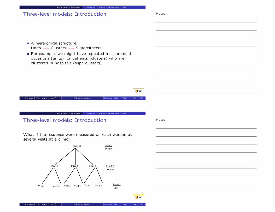
Advanced MLM topics Variance-components three-level model
Three-level models: Introduction
A hierarchical structure:Units −→ Clusters −→ Superclusters
For example, we might have repeated measurementoccasions (units) for patients (clusters) who areclustered in hospitals (superclusters).
Abdous & Duchesne (Laval) MLM-Workshop October 17-21, 2010 173 / 297
Advanced MLM topics Variance-components three-level model
Three-level models: Introduction
What if the response were measured on each woman atseveral visits at a clinic?
District
FSW 1 FSW 2 FSW 3
Level 3
Level 2Woman
Visit 1 Visit 2 Visit 1Visit 3Visit 2 Visit 3 Level 1Visit
District
Abdous & Duchesne (Laval) MLM-Workshop October 17-21, 2010 174 / 297
Notes
Notes

Advanced MLM topics Variance-components three-level model
Three-level models: Introduction
We could think of other examples with 3 levels using thecurrent IBBA round 1 data. For example:
Level 1: FSW
Level 2: District
Level 3: State
Warning: To estimate level 3 variance parameters, we needto have several level 3 units (e.g., several states)!
Abdous & Duchesne (Laval) MLM-Workshop October 17-21, 2010 175 / 297
Advanced MLM topics Variance-components three-level model
Three-level models : continuousresponses
Abdous & Duchesne (Laval) MLM-Workshop October 17-21, 2010 176 / 297
Notes
Notes

Advanced MLM topics Variance-components three-level model
Variance-components model 6
Example: Do peak-expiratory-flow measurements varybetween method?Peak expiratory flow is measured using two methods, thestandard Wright peak flow and the Mini Wright meter, eachon two occasions on 17 subjects.
Level 1: Occasion (i)
Level 2: Method (j)
Level 3: Subjects (k)
6From: MLMUS2, Chapter 2Abdous & Duchesne (Laval) MLM-Workshop October 17-21, 2010 177 / 297
Advanced MLM topics Variance-components three-level model
Variance-components model
See MLMUS2, p.53Abdous & Duchesne (Laval) MLM-Workshop October 17-21, 2010 178 / 297
Notes
Notes

Advanced MLM topics Variance-components three-level model
Variance-components model
Let Yijk be the response of subject k for method j atoccasion i. A model with random intercept for subjects :
Model 1 : Yijk = β+ ζ(3)k + εijk
Within subjects residual :
εijk |ζ(3)k ∼N(0,θ)
Random effect of subjects (between) :
ζ(3)k ∼N(0,ψ(3))
We ignore the fact that different methods were used
Abdous & Duchesne (Laval) MLM-Workshop October 17-21, 2010 179 / 297
Advanced MLM topics Variance-components three-level model
Variance-components model : Stata code
use ./mlmus2/pefr, clear
reshape long wm wp, i(id) j(occasion)
generate i = nreshape long w, i(i) j(meth) string
sort id meth occasion
list id meth occasion w in 1/8, clean noobs
encode meth, gen(method)
recode method 2=0
Abdous & Duchesne (Laval) MLM-Workshop October 17-21, 2010 180 / 297
Notes
Notes
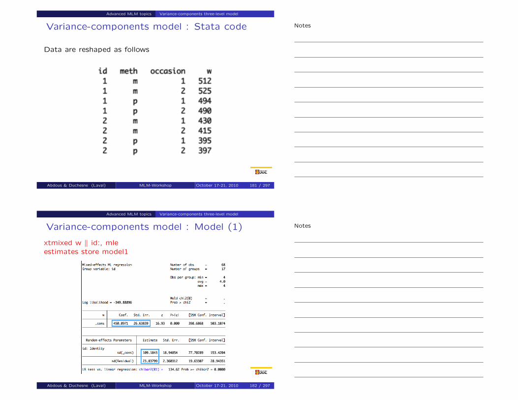
Advanced MLM topics Variance-components three-level model
Variance-components model : Stata code
Data are reshaped as follows
Abdous & Duchesne (Laval) MLM-Workshop October 17-21, 2010 181 / 297
Advanced MLM topics Variance-components three-level model
Variance-components model : Model (1)
xtmixed w ‖ id:, mleestimates store model1
Abdous & Duchesne (Laval) MLM-Workshop October 17-21, 2010 182 / 297
Notes
Notes

Advanced MLM topics Variance-components three-level model
Variance-components model
To allow for a systematic difference between the 2 methods,we might add a binary variable for estimating the methods?effect
Model 2 : Yijk = β1 +β2xj + ζ(3)k + εijk
with xj a dummy variable and
εijk |xj , ζ(3)k ∼ N(0,θ)
ζ(3)k |xj ∼ N(0,ψ(3))
Abdous & Duchesne (Laval) MLM-Workshop October 17-21, 2010 183 / 297
Advanced MLM topics Variance-components three-level model
Variance-components model : Model (2)
xtmixed w method ‖ id:, mleestimates store model2
Abdous & Duchesne (Laval) MLM-Workshop October 17-21, 2010 184 / 297
Notes
Notes

Advanced MLM topics Variance-components three-level model
Variance-components model
The intraclass correlation coefficient is the correlationbetween the 4 repeated measures on the same individual( the method used for the measurement is ignored)
ρ =ψ(3)
ψ(3) +θ=
109.222
109.222 + 23.822= 0.95
This is the % of the total variance of the measurementsthat is explained by the variance of the individualmeasurments.
Abdous & Duchesne (Laval) MLM-Workshop October 17-21, 2010 185 / 297
Advanced MLM topics Variance-components three-level model
Variance-components model
In addition to subjects and occasions variations,measurements obtained with the same method might bemore similar to each other than measurements obtained withtwo different methods
Abdous & Duchesne (Laval) MLM-Workshop October 17-21, 2010 186 / 297
Notes
Notes

Advanced MLM topics Variance-components three-level model
Variance-components of a three-level model:
The between subjects variation modeled by ζ(3)k
it reflects the fact that measurements on the samesubjects are more similar than measurements on differentsubjects.
Abdous & Duchesne (Laval) MLM-Workshop October 17-21, 2010 187 / 297
Advanced MLM topics Variance-components three-level model
Variance-components of a three-level model:
The conditional independence assumption of model (1)
Yijk = β+ ζ(3)k + εijk is violated
For a given subject, the measurements using the samemethod tend to be more similar to each other.
Abdous & Duchesne (Laval) MLM-Workshop October 17-21, 2010 188 / 297
Notes
Notes

Advanced MLM topics Variance-components three-level model
Variance-components of a three-level model:
Model 2: Yijk = β1 +β2xj + ζ(3)k + εijk is unsatisfactory
The shift of the measurements using one method relativeto the other is not constant, it varies between subjects.
Abdous & Duchesne (Laval) MLM-Workshop October 17-21, 2010 189 / 297
Advanced MLM topics Variance-components three-level model
Variance-components of a three-level model
To accommodate the between-method within-subjectheterogeneity we might add a random intercept for eachcombination of method and subject
Model 3 : Yijk = β1 + ζ(2)jk + ζ
(3)k + εijk
The random effect of method is nested within subjects: ittakes a different value for each combination method-subject
Abdous & Duchesne (Laval) MLM-Workshop October 17-21, 2010 190 / 297
Notes
Notes

Advanced MLM topics Variance-components three-level model
Variance-components of a three-level model
Interpretation of the parameters
Yijk = β1 + ζ(2)jk + ζ
(3)k + εijk
where
β1 = Population average
(across occasions, methods, and subjects)
β1 + ζ(3)k = Average for subject k
(across occasions and methods)
β1 + ζ(2)jk + ζ
(3)k = Average for method j and for subject k
(across occasions)
Abdous & Duchesne (Laval) MLM-Workshop October 17-21, 2010 191 / 297
Advanced MLM topics Variance-components three-level model
Variance-components of a three-level model
Assumptions for Model 3
Yijk = β1 + ζ(2)jk + ζ
(3)k + εijk
where
ζ(3)k |xj ∼ N(0,ψ(3))
ζ(2)jk |xj , ζ
(3)k ∼ N(0,ψ(2))
εijk |xj , ζ(2)jk , ζ
(3)k ∼ N(0,θ)
Abdous & Duchesne (Laval) MLM-Workshop October 17-21, 2010 192 / 297
Notes
Notes

Advanced MLM topics Variance-components three-level model
Variance-components model : Model (3)
xtmixed w ‖ id: ‖ method:, mleestimates store model3
Abdous & Duchesne (Laval) MLM-Workshop October 17-21, 2010 193 / 297
Advanced MLM topics Variance-components three-level model
Variance-components of a three-level model
We might add a systematic variation between methods
Model 4 : Yijk = β1 +β2xj + ζ(2)jk + ζ
(3)k + εijk
Two-way mixed-effects ANOVA model:
Two factors: method (fixed) and subject (random)
Replicates: occasion
Main effects: Method (β2), Subject (ζ(3)k )
Interaction : Method by Subject (ζ(2)jk )
Abdous & Duchesne (Laval) MLM-Workshop October 17-21, 2010 194 / 297
Notes
Notes

Advanced MLM topics Variance-components three-level model
Variance-components model : Model (4)
xtmixed w method ‖ id: ‖ method:, mleestimates store model4
Abdous & Duchesne (Laval) MLM-Workshop October 17-21, 2010 195 / 297
Advanced MLM topics Variance-components three-level model
Variance-components three-level model
Intraclass correlations for pairs of responses
Same subject k but different methods j and j ′:
ρ(subject)≡Cor (Yijk ,Yi ′j ′k |xj ,xj ′) =ψ(3)
ψ(2) +ψ(3) +θ
Same subject k and same method j :
ρ(method,subject)≡Cor (Yijk ,Yi ′jk )|xj) =ψ(2) +ψ(3)
ψ(2) +ψ(3) +θ
Abdous & Duchesne (Laval) MLM-Workshop October 17-21, 2010 196 / 297
Notes
Notes

Advanced MLM topics Variance-components three-level model
Variance-components model
Note that ρ(method,subject) > ρ(subject)Measurements for the same subject are more correlated ifthey use the same method than if they use different methods
Abdous & Duchesne (Laval) MLM-Workshop October 17-21, 2010 197 / 297
Advanced MLM topics Variance-components three-level model
Variance-components three-level model
Three-stage formulation
Stage 1: Level-1 model
Yijk = η1jk + εijk
where η1jk varies between methods j and subjects k.
Stage 2: Level-2 model
η1jk = π11k +π12xj + ζ(2)jk
where the intercept π11k is in turn modeled using thelevel-3 model.
Stage 3: Level-3 model
π11k = γ111 + ζ(3)k
Abdous & Duchesne (Laval) MLM-Workshop October 17-21, 2010 198 / 297
Notes
Notes

Advanced MLM topics Variance-components three-level model
Variance-components three-level model
Upon substituting π11k into level-2 model, and η1jk intoLevel-1 model we end up with
Yijk = γ111︸︷︷︸β1
+ π12︸︷︷︸β2
xj + ζ(2)jk + ζ
(3)k + εijk
Abdous & Duchesne (Laval) MLM-Workshop October 17-21, 2010 199 / 297
Advanced MLM topics Variance-components three-level model
Variance-components three-level model :summary
Two-Level models Three-Level modelsModel 1 Model 2 Model 3 Model 4Est (SE) Est (SE) Est (SE) Est (SE)
Fixed partβ1 450.9(26.6) 447.9(26.8) 450.9(26.6) 447.9(26.9)β2 6.0(5.7) 6.0(7.8)Random part√ψ(2) 19.5 19.0√ψ(3) 109.2 109.2 108.6 108.6√θ 23.8 23.6 17.8 17.8
Log Likelihood -349.89 -349.34 -345.29 -345.00
Abdous & Duchesne (Laval) MLM-Workshop October 17-21, 2010 200 / 297
Notes
Notes

Advanced MLM topics Variance-components three-level model
Variance-components three-level model :Comparison of Model 2 and Model 4
Thus, a random effect for methods is requiredHowever, the fixed effect β2 is not significant at 5%
Abdous & Duchesne (Laval) MLM-Workshop October 17-21, 2010 201 / 297
Advanced MLM topics Variance-components three-level model
Variance-components three-level model : Thefinal Model
xtmixed w ‖ id: ‖ method:, mle
Abdous & Duchesne (Laval) MLM-Workshop October 17-21, 2010 202 / 297
Notes
Notes

Advanced MLM topics Variance-components three-level model
Variance-components three-level model
Intraclass correlations for pairs of responses
Same subject k but different methods j and j ′:
ρ(subject) =ψ(3)
ψ(2) +ψ(3) +θ= 0.94
Same subject k and same method j :
ρ(method,subject) =ψ(2) +ψ(3)
ψ(2) +ψ(3) +θ= 0.97
Abdous & Duchesne (Laval) MLM-Workshop October 17-21, 2010 203 / 297
Advanced MLM topics Variance-components three-level model
Variance-components three-level model
In summary
No evidence of systematic bias between methods
Subject by method interaction bias
Subject-specific bias
Methods have good test-retest reliability(ρ(method,subject))
Abdous & Duchesne (Laval) MLM-Workshop October 17-21, 2010 204 / 297
Notes
Notes
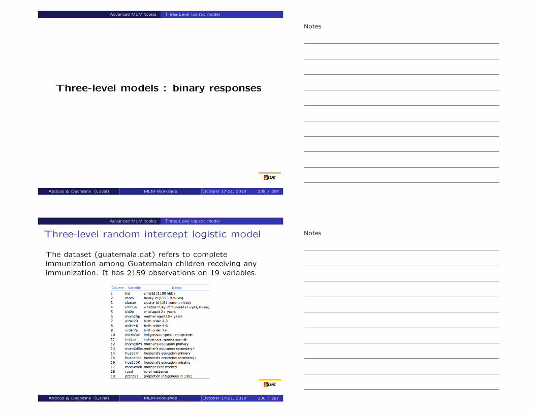
Advanced MLM topics Three-Level logistic model
Three-level models : binary responses
Abdous & Duchesne (Laval) MLM-Workshop October 17-21, 2010 205 / 297
Advanced MLM topics Three-Level logistic model
Three-level random intercept logistic model
The dataset (guatemala.dat) refers to completeimmunization among Guatemalan children receiving anyimmunization. It has 2159 observations on 19 variables.
Abdous & Duchesne (Laval) MLM-Workshop October 17-21, 2010 206 / 297
Notes
Notes

Advanced MLM topics Three-Level logistic model
Three-level random intercept logistic model
Level 1: child i- immun: indicator (yijk ) is 1 if child has received full
immunization, 0 otherwise- kid2p: dummy variable (x2ijk ) is the indicator that the
child is at least 2 years old and hence eligible for full setof immunizations
Level 2: mother j, several mother-level covariates(x3ij–x9ij)
- mom: identifier for mothers- indNoSpa: mother is indigenous, not Spanish speaking
(x3jk )- indSpa: mother is indigenous, Spanish speaking (x4jk )- . . .
Level 3: community, k, two community-level covariates,rural (x10k), pcInd81 (x11k)
Abdous & Duchesne (Laval) MLM-Workshop October 17-21, 2010 207 / 297
Advanced MLM topics Three-Level logistic model
Three-level random intercept logistic model
Children i nested in mothers j who are nested incommunities k
logit{P(yijk = 1|xijk , ζ(2)jk , ζ
(3)k )} =
(β1 + ζ(2)jk + ζ
(3)k ) +β2x2ijk + · · ·+β11x11k ,
where
xijk = (x2ijk , . . . ,x11k )′ is a vector of all covariates
ζ(3)k |xijk ∼N(0,ψ(3)) a random-intercept varying over
communities
ζ(2)jk |ζ
(3)k ,xijk ∼N(0,ψ(2)) a random-intercept varying over
mothers
random effects are assumed independent.
Abdous & Duchesne (Laval) MLM-Workshop October 17-21, 2010 208 / 297
Notes
Notes

Advanced MLM topics Three-Level logistic model
Latent-response formulation
As usual, there is a latent-response representation of thismodel:
y ∗ijk = β0 + ζ(2)jk + ζ
(3)k
+β1x1ijk + · · ·+β11x11k + εijk ,
where εijk |ζ(3)k , ζ
(2)jk ,xijk follows a standard logistic distribution
(with variance =π2/3 = 3.29), and
yijk =
{1 if y ∗ijk > 0 ;
0 if y ∗ijk ≤ 0 ;
Abdous & Duchesne (Laval) MLM-Workshop October 17-21, 2010 209 / 297
Advanced MLM topics Three-Level logistic model
Intra-class correlations
There are a couple of ways to define and compute intra-classcorrelation in a three-level random intercept logistic model:
Children from same community, different mothers:
corr(y ∗ijk ,y∗i ′j ′k |xijk ,xij ′k ′) =
ψ(3)
ψ(2) +ψ(3) + 3.29
Children from same community and mother:
corr(y ∗ijk ,y∗i ′jk |xijk ,xijk ′) =
ψ(2) +ψ(3)
ψ(2) +ψ(3) + 3.29
In these models ψ(2),ψ(3) > 0⇒ children from a same motherare more correlated than children from a same communitybut different mothers.
Abdous & Duchesne (Laval) MLM-Workshop October 17-21, 2010 210 / 297
Notes
Notes

Advanced MLM topics Three-Level logistic model
Three-stage formulation
Stage 1: Level-1 : Child-Level : x2ijk
logit{P(yijk = 1|xijk , ζ(2)jk , ζ
(3)k )} = η1jk + β2x2ijk︸ ︷︷ ︸
Level−1var .
where the intercept η1jk varies between mothers j andcommunities k.
Abdous & Duchesne (Laval) MLM-Workshop October 17-21, 2010 211 / 297
Advanced MLM topics Three-Level logistic model
Three-stage formulation
Stage 2: Level-2 : mother-level: 7 variables w2jk , . . . ,w8jk
η1jk = π11k +π12w2jk + · · ·+π18w8jk︸ ︷︷ ︸Level−2var .
+ζ(2)jk
the intercept π11k is in turn modeled using thecommunity-level (level-3) model.
Abdous & Duchesne (Laval) MLM-Workshop October 17-21, 2010 212 / 297
Notes
Notes

Advanced MLM topics Three-Level logistic model
Three-stage formulation
Stage 3: Level-3 : community-level model : v2k = rural,v3k = pcInd81
π11k = γ111 +γ112v2k +γ113v3k︸ ︷︷ ︸Level−3var .
+ζ(3)k
Substitute step-3 in step-2 then step-2 in step-1
Abdous & Duchesne (Laval) MLM-Workshop October 17-21, 2010 213 / 297
Advanced MLM topics Three-Level logistic model
Fitting three-level random intercept logisticmodel in Stata
This can be done using either xtmelogit or gllamm. We willillustrate using the Guatemalan immunization study.
First we must download the data
* get the data from Stata website
use http://www.stata-press.com/data/mlmus2/guatemala, clear
* save to local file for future use
save "F:\Data-Stata\guatemala.dta", replace
Abdous & Duchesne (Laval) MLM-Workshop October 17-21, 2010 214 / 297
Notes
Notes

Advanced MLM topics Three-Level logistic model
three-level random interceptlogistic model with gllamm
Abdous & Duchesne (Laval) MLM-Workshop October 17-21, 2010 215 / 297
Advanced MLM topics Three-Level logistic model
Fitting three-level random intercept logisticmodel with gllamm
Download gllamm fromhttp://www.gllamm.org/install.html or simply usessc install gllamm
Use gllamm with 5 quadrature points (...otherwise, timeconsuming...)
gllamm immun kid2p indNoSpa indSpa momEdPri momEdSec husEdPri ///
husEdSec husEdDK rural pcInd81, ///
family(binomial) link(logit) i(mom cluster) nip(5)
Abdous & Duchesne (Laval) MLM-Workshop October 17-21, 2010 216 / 297
Notes
Notes

Advanced MLM topics Three-Level logistic model
Fitting three-level random intercept logisticmodel with gllamm
Abdous & Duchesne (Laval) MLM-Workshop October 17-21, 2010 217 / 297
Advanced MLM topics Three-Level logistic model
Fitting three-level random intercept logisticmodel with gllamm
Store the previous estimates in order to use them asstarting valuesmatrix a=e(b)
Increase the number of quadrature points to 8 (default)per dimension + adaptive quadraturegllamm immun kid2p indNoSpa indSpa momEdPri momEdSec husEdPri ///
husEdSec husEdDK rural pcInd81, ///
family(binomial) link(logit) i(mom cluster) from(a) adapt
Abdous & Duchesne (Laval) MLM-Workshop October 17-21, 2010 218 / 297
Notes
Notes

Advanced MLM topics Three-Level logistic model
Fitting three-level random intercept logisticmodel with gllamm
Abdous & Duchesne (Laval) MLM-Workshop October 17-21, 2010 219 / 297
Advanced MLM topics Three-Level logistic model
Fitting three-level random intercept logisticmodel with gllamm
Same results for ”odds ratios”: gllam, eform
Abdous & Duchesne (Laval) MLM-Workshop October 17-21, 2010 220 / 297
Notes
Notes

Advanced MLM topics Three-Level logistic model
Three-level random intercept logistic model,Guatemalan immunization
The variable of main interest x2ijk =kid2p has a large OR5.55> 0 and is highly significant.
The variance of the mother-level random intercepts isψ(2) = 5.19.
The variance of the community-level random intercepts isψ(3) = 1.03.
Abdous & Duchesne (Laval) MLM-Workshop October 17-21, 2010 221 / 297
Advanced MLM topics Three-Level logistic model
Three-level random intercept logistic model,Guatemalan immunization
The correlation between the latent-responses of two childrenfrom a same community but from different mothers is
ψ(3)/(ψ(2) + ψ(3) + 3.29) = 1.03/(5.19 + 1.03 + 3.29) = 0.11.
The correlation between the latent-responses of two childrenfrom a same mother is
(ψ(2) +ψ(3))/(ψ(2) +ψ(3) +3.29) = (5.19+1.03)/(5.19+1.03+3.29) = 0.65.
Abdous & Duchesne (Laval) MLM-Workshop October 17-21, 2010 222 / 297
Notes
Notes

Advanced MLM topics Three-Level logistic model
three-level random interceptlogistic model with xtmelogit
Abdous & Duchesne (Laval) MLM-Workshop October 17-21, 2010 223 / 297
Advanced MLM topics Three-Level logistic model
Fitting three-level random intercept logisticmodel with xtmelogit
Start with Laplace method obtained with the optionintpoints(1) or laplace which is computationallyefficient.** 10.7.2 Using xtmelogit
* Laplace
xtmelogit immun kid2p indNoSpa indSpa momEdPri momEdSec ///
husEdPri husEdSec husEdDK rural pcInd81 ///
|| cluster: || mom:, intpoints(1)
Save these Laplace estimates in order to use them asstarting values for MLE with adaptive quadrature with 3or 4 or 5 integration points....TIME consuming...
matrix a = e(b)
Abdous & Duchesne (Laval) MLM-Workshop October 17-21, 2010 224 / 297
Notes
Notes

Advanced MLM topics Three-Level logistic model
Fitting three-level random intercept logisticmodel with xtmelogit
Laplace estimates
Abdous & Duchesne (Laval) MLM-Workshop October 17-21, 2010 225 / 297
Advanced MLM topics Three-Level logistic model
Fitting three-level random intercept logisticmodel with xtmelogit
Adaptive quadrature: 5 points
matrix a = e(b)
xtmelogit immun kid2p indNoSpa indSpa momEdPri momEdSec husEdPri husEdSec ///
husEdDK rural pcInd81 || cluster: || mom:, intpoints(5) ///
from(a) refineopts(iterate(0))
Abdous & Duchesne (Laval) MLM-Workshop October 17-21, 2010 226 / 297
Notes
Notes

Advanced MLM topics Three-Level logistic model
Fitting three-level random intercept logisticmodel with xtmelogit
Adaptive quadrature: 5 points
Abdous & Duchesne (Laval) MLM-Workshop October 17-21, 2010 227 / 297
Advanced MLM topics Three-Level logistic model
Fitting three-level random intercept logisticmodel with xtmelogit
Adaptive quadrature: 8 points
Abdous & Duchesne (Laval) MLM-Workshop October 17-21, 2010 228 / 297
Notes
Notes

Advanced MLM topics Three-Level logistic model
Fitting three-level random intercept logisticmodel with xtmelogit
Abdous & Duchesne (Laval) MLM-Workshop October 17-21, 2010 229 / 297
Advanced MLM topics Three-Level logistic model
Three-level random coefficientlogistic model
Abdous & Duchesne (Laval) MLM-Workshop October 17-21, 2010 230 / 297
Notes
Notes

Advanced MLM topics Three-Level logistic model
Three-level random coefficient logistic model
It is possible to let the coefficients in front of level 1(Child) variables vary from level 2 to level 2 (Mother )and/or from level 3 to level 3 unit (Community).
Similarly, it is possible to let the coefficients in front oflevel 2 variables vary from level 3 to level 3 unit.
In the Guatemalan immunization study, does the effectof eligibility (level 1 variable x2ijk) vary from communityto community (level 3 units)?
Abdous & Duchesne (Laval) MLM-Workshop October 17-21, 2010 231 / 297
Advanced MLM topics Three-Level logistic model
Three-level random coefficient logistic model
We can refit the model, but with a random coefficient thatvaries across level 3 units in front of x2ijk :
logit{P(yijk = 1|xijk , ζ(2)jk , ζ
(3)k )} = β1 + ζ
(2)jk + ζ
(3)1k
+ (β2 + ζ(3)2k )x2ijk
+β3x3jk · · ·+β11x11k ,
where (ζ(3)1k , ζ
(3)2k )|xijk ∼N[(0,0),Ψ(3)]
with
Ψ(3) =
[ψ
(3)11 ) ψ
(3)12 )
ψ(3)21 ) ψ
(3)22 )
]
and ζ(2)jk |ζ
(3)0k , ζ
(3)2k ,xijk ∼N(0,ψ(2)).
Abdous & Duchesne (Laval) MLM-Workshop October 17-21, 2010 232 / 297
Notes
Notes

Advanced MLM topics Three-Level logistic model
Three-level random coefficient logistic model
�
Normally if a random coefficient is included at acertain level, corresponding random coefficients should alsobe included at all lower levels.
In the Guatemalan immunization example, this has beendone for the intercepts, but not for the coefficient of x2ijk
because the treatment was applied at the community leveland x2ijk does not vary much at the mother-level (seeMLMUS2 p. 454 for detailed discussion).
Abdous & Duchesne (Laval) MLM-Workshop October 17-21, 2010 233 / 297
Advanced MLM topics Three-Level logistic model
Fitting three-level random coefficient logisticmodel with gllamm
First, fit a random-intercept model
logit{P(yijk = 1|xijk , ζ(2)jk , ζ
(3)k )} =
β1 +β2x2ijk +β10x10k +β11x11kζ(2)jk + ζ
(3)k
Use the previous model to retrieve the estimations of thefull model : estimates restore glri8 and the skip optionsince some covariates have been dropped
matrix a = e(b)
gllamm immun kid2p rural pcInd81, ///
family(binomial) link(logit) ///
i(mom cluster) from(a) skip adapt eform
estimates store glri0
Abdous & Duchesne (Laval) MLM-Workshop October 17-21, 2010 234 / 297
Notes
Notes

Advanced MLM topics Three-Level logistic model
Fitting three-level random coefficient logisticmodel with gllamm
Abdous & Duchesne (Laval) MLM-Workshop October 17-21, 2010 235 / 297
Advanced MLM topics Three-Level logistic model
Fitting three-level random coefficient logisticmodel with gllamm
Specify equation for intercept (one for community leveland one for mother level) and a slope for kid2p atcommunity levelgenerate cons = 1
eq inter: cons
eq slope: kid2p
Use previous estimates as starting values + two morevalues (for ψ(3)
22 and ψ(3)21 )
matrix a = e(b)
matrix a = (a,.2,0)
Abdous & Duchesne (Laval) MLM-Workshop October 17-21, 2010 236 / 297
Notes
Notes

Advanced MLM topics Three-Level logistic model
Fitting three-level random coefficient logisticmodel with gllamm
gllamm immun kid2p rural pcInd81, ///
family(binomial) link(logit) i(mom cluster) ///
nrf(1 2) eqs(inter inter slope) nip(8 4 4) ///
from(a) copy adapt eform
estimates store glrc
The nrf() option specifies the number of random levelsin i() statement: nrf(1 2) means 1 for mom and 2 forcluster
The eqs() option specifies one equation for each randomeffect
The nip() option specifies the number of quadraturepoints for each random effect
Abdous & Duchesne (Laval) MLM-Workshop October 17-21, 2010 237 / 297
Advanced MLM topics Three-Level logistic model
Fitting three-level random coefficient logisticmodel with gllamm
Abdous & Duchesne (Laval) MLM-Workshop October 17-21, 2010 238 / 297
Notes
Notes

Advanced MLM topics Three-Level logistic model
Three-level random coefficient model,Guatemalan immunization
The random-intercept variance at level 3 is ψ(3)11 = 2.42, it
might be interpreted as the residual between-communityvariance for too young children (kid2p=0)
The random-slope variance at level 3 is ψ(3)22 = 1.80, it
might be interpreted as the residual variability in theeffectiveness of the campaign across communities.
Abdous & Duchesne (Laval) MLM-Workshop October 17-21, 2010 239 / 297
Advanced MLM topics Three-Level logistic model
Three-level random coefficient model,Guatemalan immunization
The negative covariance (ψ(3)12 =−1.51) or correlation
(ψ(3)12 /
√ψ
(3)11 ψ
(3)22 =−1.51/
√2.41×1.79 =−0.73) between
the random intercept and coefficient at level 3 suggeststhat effect of kid2p is stronger in communities where theimmunization rate is low.
Interactions between kid2p and level 3 covariates may beable to explain part of the variability in the randomcoefficients.
Abdous & Duchesne (Laval) MLM-Workshop October 17-21, 2010 240 / 297
Notes
Notes

Advanced MLM topics Three-Level logistic model
Fitting three-level random coefficient logisticmodel with gllamm
lrtest glrc glri0 =⇒ LRchi2(2) = 8.43 andProb > chi2 = 0.0148
Abdous & Duchesne (Laval) MLM-Workshop October 17-21, 2010 241 / 297
Advanced MLM topics Three-Level logistic model
Fitting three-level random coefficient logisticmodel with gllamm
xtmelogit immun kid2p rural pcInd81 ///
|| cluster:kid2p, cov(unstructured) || mom: ///
,intpoints(4 8) or
estimates store xtrc
The level 3 specification: ‖ cluster:kid2p,cov(unstructured). A random slope for kid2p, anintercept is included by default.
No restriction for the covariance matrix
Abdous & Duchesne (Laval) MLM-Workshop October 17-21, 2010 242 / 297
Notes
Notes

Advanced MLM topics Three-Level logistic model
Fitting three-level random coefficient logisticmodel with xtmelogit
Abdous & Duchesne (Laval) MLM-Workshop October 17-21, 2010 243 / 297
Advanced MLM topics Crossed random effects: continuous response
Multilevel models with crossed randomeffects
Abdous & Duchesne (Laval) MLM-Workshop October 17-21, 2010 244 / 297
Notes
Notes

Advanced MLM topics Crossed random effects: continuous response
Hierarchical structures
Abdous & Duchesne (Laval) MLM-Workshop October 17-21, 2010 245 / 297
Advanced MLM topics Crossed random effects: continuous response
Nested vs crossed random-effects
Nested design: When observations from level L aresampled (e.g., state), then the observations from levelL−1 (e.g., district) are drawn from units sampled atlevel L.
Abdous & Duchesne (Laval) MLM-Workshop October 17-21, 2010 246 / 297
Notes
Notes

Advanced MLM topics Crossed random effects: continuous response
Cross-classified structure7
7www.bristol.ac.uk/cmm/team/cross-classified-review.pdAbdous & Duchesne (Laval) MLM-Workshop October 17-21, 2010 247 / 297
Advanced MLM topics Crossed random effects: continuous response
Cross-classified structure
Abdous & Duchesne (Laval) MLM-Workshop October 17-21, 2010 248 / 297
Notes
Notes

Advanced MLM topics Crossed random effects: continuous response
Nested vs crossed random-effects
Crossed design: The fact that units from level L aresampled does not determine whether units at level L−1(e.g., Round) will be observed or not. For instanceresults from Round 1 and Round 2 will be sampledregardless of which FSW are sampled.
Abdous & Duchesne (Laval) MLM-Workshop October 17-21, 2010 249 / 297
Advanced MLM topics Crossed random effects: continuous response
Typical situations with crossed random-effects
See MLMUS2, p. 500
Panel (longitudinal) data with random time effects: theinvestment by each of 10 firms is recorded each yearfrom 1935 to 1965 (see pp. 474-480 of MLMUS2)
Observational data on individuals classified in two ways:an attainment score at age 16 is obtained from pupilswho each attended one of 148 primary schools and oneof 19 secondary schools (see pp. 481-492 of MLMUS2)
Abdous & Duchesne (Laval) MLM-Workshop October 17-21, 2010 250 / 297
Notes
Notes

Advanced MLM topics Crossed random effects: continuous response
Typical situations with crossed random-effects
Data from an experimental design with crossed blockingfactors (see pp. 493-499 of MLMUS2)
Several raters rate each of several objects (see exercises11.4 and 11.7 of MLMUS2)
Social network data (e.g., individuals rate how muchthey like every other individual)
Abdous & Duchesne (Laval) MLM-Workshop October 17-21, 2010 251 / 297
Advanced MLM topics Crossed random effects: continuous response
Example: How does investment depend onexpected profit and capital stock?
Data on 10 large American corporations : grunfeld.dta
fn: firm identifier i
firmname: firm name
yr: year j
I: Annual gross investment (in $ 1, 000, 000) = amountspent on plant and equipment, . . . (yij)
F: market value of firm (in $ 1, 000, 000) = value of allshares plus book value of all debts . . . (x2ij)
C: real vaue of capital stock (in $ 1, 000, 000) =deviation of stock of plant and equipment from stock in1933 . . . (x3ij)
Abdous & Duchesne (Laval) MLM-Workshop October 17-21, 2010 252 / 297
Notes
Notes

Advanced MLM topics Crossed random effects: continuous response
A basic cross-classified model
The gross investment yij for firm i in year j could beexpressed in terms of the market value and capital stockx2ij and x3ij :
yij = β1 +β2x2ij +β3x3ij
The investment behavior of corporations is surely notdeterministic. Allow the effect of both firms and yearson gross investment to vary:
yij = β1 +β2x2ij +β3x3ij + ζ1i + ζ2j + εij
Abdous & Duchesne (Laval) MLM-Workshop October 17-21, 2010 253 / 297
Advanced MLM topics Crossed random effects: continuous response
A basic cross-classified model
The two random intercepts ζ1i and ζ2i represent thefactors firm (i) and year (j) that are crossed instead ofnested, while εij is a residual error with
ζ1i ∼N(0,ψ1), ζ2i ∼N(0,ψ2), εij ∼N(0,θ).
The random intercept ζ1i is shared across all years for agiven firm i.
The random intercept ζ2j is shared across all firms for agiven year j.
The residual error εij = interaction between year andfirm and any other effect specific to firm i in year j
Abdous & Duchesne (Laval) MLM-Workshop October 17-21, 2010 254 / 297
Notes
Notes

Advanced MLM topics Crossed random effects: continuous response
Example: How does investment depend onexpected profit and capital stock?
�
The STATA xtmixed is designed for nested randomeffects. Use the following trick to fit crossed effects
Consider the entire dataset as a level-3 unit a (say)within which both firms and years are nested.
Choose the factor with more levels (i.e. years) as level-2
units with random intercepts u(2)ja .
Specify a level-3 random intercept for each unit of theother factor ( firm): u(3)
pa for p = 1, . . . ,10. To this end,construct the dummy variable dpij as follows
dpij =
{1 if p = i0 otherwise
Abdous & Duchesne (Laval) MLM-Workshop October 17-21, 2010 255 / 297
Advanced MLM topics Crossed random effects: continuous response
Example: investment ?
The previous model becomes
yija = β1 +β2x2ij +β3x3ij + u(2)ja +
∑p
u(3)pa dpij + εija
Abdous & Duchesne (Laval) MLM-Workshop October 17-21, 2010 256 / 297
Notes
Notes

Advanced MLM topics Crossed random effects: continuous response
Example: investment ?
Residual intra-class correlations
ρ(firm): Correlation of observations on the same firmover time
ρ(firm) = cor (yij ,yij ′ |x2ij ,x3ij ,x2ij ′ ,x3ij ′) =ψ1
ψ1 +ψ2 +θ
ρ(year ): Correlation for the same year across firms
ρ(year ) = cor (yij ,yi ′j |x2ij ,x3ij ,x2i ′j ,x3i ′j) =ψ2
ψ1 +ψ2 +θ.
Abdous & Duchesne (Laval) MLM-Workshop October 17-21, 2010 257 / 297
Advanced MLM topics Crossed random effects: continuous response
Example: investment ?
Stata code
To specify the random intercept u(3)pa for each firm use
the syntax R.fn.
R.fn sets a covariance matrix proportional to the identity(same variances and correlations=0)
The artificial level-3 identifier is created by all
use http://www.stata-press.com/data/mlmus2/grunfeld, clear
xtmixed I F C || all: R.fn || yr:, mle
Abdous & Duchesne (Laval) MLM-Workshop October 17-21, 2010 258 / 297
Notes
Notes

Advanced MLM topics Crossed random effects: continuous response
Example: investment ?
Abdous & Duchesne (Laval) MLM-Workshop October 17-21, 2010 259 / 297
Advanced MLM topics Crossed random effects: continuous response
Example: investment ?
High correlation over years within firms
ρ(firm) =ψ1
ψ1 +ψ2 +θ= 0.7
Negligible correlation over firms within years
ρ(year ) =ψ2
ψ1 +ψ2 +θ= 0.002
The syntax xtmixed I F C || all: R.yr || fn:, mle
produces the same results as above, BUT it has 20random effects at level 3
Abdous & Duchesne (Laval) MLM-Workshop October 17-21, 2010 260 / 297
Notes
Notes

Advanced MLM topics Crossed random effects: continuous response
Example: investment ?
Empirical Bayes (BLUP) preditions of the random effectsof firms and year using predict and reffects option:
** 11.3.4 Prediction
predict firm year, reffects
sort fn yr
list fn firmname yr firm year if yr<1938&fn<5, clean noobs
Abdous & Duchesne (Laval) MLM-Workshop October 17-21, 2010 261 / 297
Advanced MLM topics Crossed random effects: continuous response
Example: Primary and secondary school vsattainment at age 16
Dataset fife.dta : students cross-classified by 148primary schools and 19 secondary schools.
Pupils from a given primary school can go to several ofthe secondary schools and vice-versa =⇒ Primary andsecondary schools are not nested
Not every combination of primary and secondary schoolexists
Many combinations occur multiple times.
Abdous & Duchesne (Laval) MLM-Workshop October 17-21, 2010 262 / 297
Notes
Notes

Advanced MLM topics Crossed random effects: continuous response
Example: Primary and secondary school
attain: attainment score at age 16 of pupil i who wentto primary school k and secondary school j (yijk)
pid: identifier of primary school (up to age 12) (k)
sid: identifier of secondary school (from age 12) (j)
vrq: verbal-reasoning score (last year of primary school)
sex: 1: female, 0: male
Abdous & Duchesne (Laval) MLM-Workshop October 17-21, 2010 263 / 297
Advanced MLM topics Crossed random effects: continuous response
A look at the data structure
Create dummy variables for each combination of primaryand secondary schools
egen pick_comb = tag(pid sid)
Compute the number of such combinations by primaryschools and list them
egen numsid = total(pick_comb), by(pid)
sort pid sid
list pid sid numsid if pick_comb & pid<10, sepby(pid) noobs
Abdous & Duchesne (Laval) MLM-Workshop October 17-21, 2010 264 / 297
Notes
Notes

Advanced MLM topics Crossed random effects: continuous response
A look at the data structure
Abdous & Duchesne (Laval) MLM-Workshop October 17-21, 2010 265 / 297
Advanced MLM topics Crossed random effects: continuous response
Additive crossed random-effects model
A simple model with random intercepts for primary andsecondary schools is
yijk = β1 + ζ1j + ζ2k + εijk ,
where εijk , ζ1j , ζ2k are independent and normally distributedwith mean 0 and respective variances θ, ψ1 and ψ2.
Abdous & Duchesne (Laval) MLM-Workshop October 17-21, 2010 266 / 297
Notes
Notes

Advanced MLM topics Crossed random effects: continuous response
Additive crossed random-effects model
We can rewrite the model as a three-level model with nestedrandom effects:
Level 3: the entire dataset is the only level 3 unit
Level 2: treat one of the two crossed factors as level 2(usually the factor with more levels) and put a level 2
random intercept in the model, say u(2)j
Level 1: Define a dummy variable dpjk that will be 1 ifp = k, 0 otherwise and put a level-3 random coefficientu(3)
p in front of dpjk in the model
Abdous & Duchesne (Laval) MLM-Workshop October 17-21, 2010 267 / 297
Advanced MLM topics Crossed random effects: continuous response
Additive crossed random-effects model
The model:
yijk = β1 + u(2)j +
∑p
u(3)p dpjk + εijk
We have 19 SS and 148 PS =⇒ Level-2 Units: Primaryschool, Level-3: artificial level (dataset) + 19 randomeffects for the SS
Stata code
** 11.5.2 Estimation using xtmixed
xtmixed attain || _all: R.sid || pid:, mle variance
estimates store model1
Abdous & Duchesne (Laval) MLM-Workshop October 17-21, 2010 268 / 297
Notes
Notes

Advanced MLM topics Crossed random effects: continuous response
Additive crossed random-effects model
Abdous & Duchesne (Laval) MLM-Workshop October 17-21, 2010 269 / 297
Advanced MLM topics Crossed random effects: continuous response
Intra-class correlations
Within primary school:ψ2/(ψ1 +ψ2 +θ) = 1.12/(0.35 + 1.12 + 8.11) = 0.12
Within secondary school:ψ1/(ψ1 +ψ2 +θ) = 0.35/(0.35 + 1.12 + 8.11) = 0.037
θ captures variation unexplained by primary school orsecondary school effects (e.g., pupil-level effects, covariates,interaction between primary and secondary school).
Abdous & Duchesne (Laval) MLM-Workshop October 17-21, 2010 270 / 297
Notes
Notes

Advanced MLM topics Crossed random effects: continuous response
Additive crossed random-effects model withrandom interaction
Since we have more than one pupil in mostprimary-secondary school combination, we can fit a modelwith a random interaction:
yijk = β1 + ζ1j + ζ2k + ζ3jk + εijk ,
with εijk , ζ1j , ζ2k , ζ3jk independent and normally distributedwith mean 0 and respective variances θ, ψ1, ψ2 and ψ3.
⇒ The effect of a secondary school is now allowed todepend on which primary school the pupil attended (whereasit was the same regardless of the primary school attended inthe previous model).
Abdous & Duchesne (Laval) MLM-Workshop October 17-21, 2010 271 / 297
Advanced MLM topics Crossed random effects: continuous response
Additive crossed random-effects model withrandom interaction
Severall residual intra-class correlations :Residual correlation between pupils from different PSsbut from the same SS
ρ(j) = ρ(SS) = cor (yijk ,yi ′jk ′) =ψ1
ψ1 +ψ2 +ψ3 +θ
Residual correlation between pupils from different SSsbut from the same PS
ρ(k) = ρ(PS) = cor (yijk ,yi ′j ′k ) =ψ2
ψ1 +ψ2 +ψ3 +θ
Residual correlation between pupils from the sameprimary and SS
ρ(jk) = ρ(SS,PS) = cor (yijk ,yi ′jk ) =ψ1 +ψ2 +ψ3
ψ1 +ψ2 +ψ3 +θ
Abdous & Duchesne (Laval) MLM-Workshop October 17-21, 2010 272 / 297
Notes
Notes

Advanced MLM topics Crossed random effects: continuous response
Additive crossed random-effects model withrandom interaction
If we consider all pupils in SS j, what is the residualcorrelation between pupils from the same PS?
ρ(k |j) = ρ(PS|SS) = cor (yijk ,yi ′jk |j) =ψ2 +ψ3
ψ2 +ψ3 +θ
If we consider all pupils in PS k, what is the residualcorrelation between pupils from the same SS?
ρ(j|k) = ρ(SS|PS) = cor (yijk ,yi ′jk |k) =ψ1 +ψ3
ψ1 +ψ3 +θ
Abdous & Duchesne (Laval) MLM-Workshop October 17-21, 2010 273 / 297
Advanced MLM topics Crossed random effects: continuous response
Fitting the model with random interactionwith xtmixed
Two ways to fit the model
Create an identifier variable for SS and SP combinations
egen comb=group(sid pid)
xtmixed attain || _all: R.sid || pid: || comb: ///
, mle variance
Since sid is nested within pid, we do not need to createcomb
egen comb=group(sid pid)
xtmixed attain || _all: R.sid || pid: || sid: ///
, mle variance
estimates store model2
Abdous & Duchesne (Laval) MLM-Workshop October 17-21, 2010 274 / 297
Notes
Notes

Advanced MLM topics Crossed random effects: continuous response
Model with random interaction
Abdous & Duchesne (Laval) MLM-Workshop October 17-21, 2010 275 / 297
Advanced MLM topics Crossed random effects: continuous response
Intra-class correlations
Within primary school:ψ2/(ψ1 +ψ2 +ψ3 +θ) = 0.90/(0.31+0.90+0.24+8.09) = 0.09
Within secondary school:ψ1/(ψ1 +ψ2 +θ) = 0.31/(0.31 + 0.90 + 0.24 + 8.09) = 0.032
Same primary & secondary:(ψ1 +ψ2 +ψ3)/(ψ1 +ψ2 +θ) =(0.31 + 0.90 + 0.24)/(0.31 + 0.90 + 0.24 + 8.09) = 0.15
primary|secondary: (ψ2 +ψ3)/(ψ2 +ψ3 +θ) =(0.90 + 0.24)/(0.90 + 0.24 + 8.09) = 0.12
secondary|primary: (ψ1 +ψ3)/(ψ1 +ψ3 +θ) =(0.31 + 0.24)/(0.31 + 0.24 + 8.09) = 0.06
Abdous & Duchesne (Laval) MLM-Workshop October 17-21, 2010 276 / 297
Notes
Notes

Advanced MLM topics Crossed random effects: continuous response
Is the interaction needed?
A likelihood ratio test can be used to see whether theinteraction is significant (but since this tests if ψ3 = 0, thep-value is conservative and should be divided by 2.
The stata code lrtest model1 model2 gives a p-value of 0.28(0.14 when divided by 2), so the interaction is notsignificant.
Abdous & Duchesne (Laval) MLM-Workshop October 17-21, 2010 277 / 297
Advanced MLM topics Crossed random effects: logistic regression
Crossed random-effects: logisticregression
Abdous & Duchesne (Laval) MLM-Workshop October 17-21, 2010 278 / 297
Notes
Notes

Advanced MLM topics Crossed random effects: logistic regression
Crossed random-effects: logistic regression
We can fit a similar model to the data when the response isbinary. In this case, the model becomes
logit{P[yijk = 1|xijk , ζ1j , ζ2k ]} = β1 +β′2xijk + ζ1j + ζ2k ,
with ζ1j , ζ2k independent and normally distributed withmean 0 and respective variances ψ1 and ψ2.
Abdous & Duchesne (Laval) MLM-Workshop October 17-21, 2010 279 / 297
Advanced MLM topics Crossed random effects: logistic regression
Latent-response formulation
Once again, we can obtain the model from the precedingpage when we observe yijk = 1 if y ∗ijk > 0 and yijk = 0 ify ∗ijk ≤ 0, with
y ∗ijk = β1 +β′2xijk + ζ1j + ζ2k + εijk ,
with ζ1j , ζ2k independent and normally distributed withmean 0 and respective variances ψ1 and ψ2 and εijk followinga standard logistic distribution.
Abdous & Duchesne (Laval) MLM-Workshop October 17-21, 2010 280 / 297
Notes
Notes

Advanced MLM topics Crossed random effects: logistic regression
Crossed random-effects: logistic regression
Residual intra-class correlations between latent-responses aregiven by
ρ(j) =ψ1
ψ1 +ψ2 + 3.29
ρ(k) =ψ2
ψ1 +ψ2 + 3.29.
Abdous & Duchesne (Laval) MLM-Workshop October 17-21, 2010 281 / 297
Advanced MLM topics Crossed random effects: logistic regression
Crossed random-effects: logistic regression
Do salamanders from different populations matesuccessfully? (MLMUS2, p. 493)
Two salamander populations: roughbutt (RB) andwhiteside (WS) which had been geographically isolatedfrom each other.
Scope: Investigate whether salamanders wouldcross-breed.
Three experiment have been conducted : 1 in 1986 and2 in 1987.
Abdous & Duchesne (Laval) MLM-Workshop October 17-21, 2010 282 / 297
Notes
Notes

Advanced MLM topics Crossed random effects: logistic regression
Salamanders data: design
Experiment 1 in 1986: two groups of 20 salamanders
Each group = 5 RB male (RBM), 5 RB female (RBF),5 WS male (WSM) and 5 WS female (WSF).
Within each group: 60 male-female pairs. Eachsalamander has 3 partners from the same population and3 from the other population.
Experiment 2 in 1987: The same salamanders as inExperiment 1
Experiment 3 in 1987: new set of salamanders
Abdous & Duchesne (Laval) MLM-Workshop October 17-21, 2010 283 / 297
Advanced MLM topics Crossed random effects: logistic regression
Salamanders data: design
Abdous & Duchesne (Laval) MLM-Workshop October 17-21, 2010 284 / 297
Notes
Notes

Advanced MLM topics Crossed random effects: logistic regression
Salamanders data: variables
y: indicator for successful mating (1: successful, 0:unsuccessful)
female: male identifier 1-60
male : female identifier 1-60
group: identifier of 6 groups of 20 salamanders (seetable 11-4)
experiment: experimnet number (1-3)
rbm rbf wsm wsf: dummy variables for salamander type
Abdous & Duchesne (Laval) MLM-Workshop October 17-21, 2010 285 / 297
Advanced MLM topics Crossed random effects: logistic regression
Salamanders data: design
Abdous & Duchesne (Laval) MLM-Workshop October 17-21, 2010 286 / 297
Notes
Notes

Advanced MLM topics Crossed random effects: logistic regression
Salamanders data: design
Abdous & Duchesne (Laval) MLM-Workshop October 17-21, 2010 287 / 297
Advanced MLM topics Crossed random effects: logistic regression
Crossed random-effects: logistic regression
Treat salamanders from experiment 1 and 2 as independentand fit a logistic random-effects regression model
logit{P[yij = 1|x2i ,x3j , ζ1i , ζ2j ]} =
β1 +β2x2i +β3x3j +β4x2ix3j + ζ1i + ζ2j ,
where
ζ1i and ζ2j are independent random intercepts for males iand females j with variances ψ1 and ψ2 (givencovariates).
The covariates wsm (x2i ) and wsf (x3j) and theirinteraction are included
Abdous & Duchesne (Laval) MLM-Workshop October 17-21, 2010 288 / 297
Notes
Notes

Advanced MLM topics Crossed random effects: logistic regression
Fitting the model with xtmelogit
This is done in exactly the same manner as with xtmixed.xtmelogit y wsm wsf ww || all: R.male || female:,
orxtmelogit y wsm wsf ww || all: R.female || male:,
Unfortunately, it is computationally extremelydemanding. In both cases we need 60 randomcoefficients.
Abdous & Duchesne (Laval) MLM-Workshop October 17-21, 2010 289 / 297
Advanced MLM topics Crossed random effects: logistic regression
Fitting the model with xtmelogit
How to set up the crossed-random effects model for ahierarchical software package?
See Harvey Goldstein Chapter 8,Multilevel StatisticalModels Second Edition. (London: Edward Arnold,1995), esp. pp. 116-17 and pp. 123-24.)
Choose one of the crossed random effects as the secondlevel
Take the other crossed effect and create dummy(indicator) variables of it as random effects at a thirdlevel.
Constraint the variance-covariance matrix of this secondrandom effect to be proportional to the identity(diagonal elements are equal and off-diagonal elementsare zero)
Abdous & Duchesne (Laval) MLM-Workshop October 17-21, 2010 290 / 297
Notes
Notes

Advanced MLM topics Crossed random effects: logistic regression
Fitting the model with xtmelogit
In chapter 11 of MLMUS2, interested readers can find atrick to partition the data so that numerical integrationis performed in lower dimension.
It requires the use of the Stata command supclust.
This trick cannot always be applied: it can only be usedwhen the data can be partitioned into clusters withinwhich other factors are nested.
split the data on primary/secondary schools into 3“regions” so that all primary and secondary schools (i)appear in a single region and (ii) a secondary school withwhich a primary school is paired must be in the sameregion.
Abdous & Duchesne (Laval) MLM-Workshop October 17-21, 2010 291 / 297
Advanced MLM topics Crossed random effects: logistic regression
Fitting the model with xtmelogit
Since Salamanders are nested within groups with nomatings occurring across groups, we can use group asthe highest level.
We only need 10 random coefficients for males
The first random coefficient is for a dummy variablecorresponding to the male salamanders number: 1, 11,21, 31,41 and 51.
The second random coefficient is for a dummy variablecorresponding to the male salamanders number: 2, 12,22, 32, 42 and 52.
and so forth.
Groups of 6 salamanders with different randomcoefficients (each group has its own coefficient)
Abdous & Duchesne (Laval) MLM-Workshop October 17-21, 2010 292 / 297
Notes
Notes

Advanced MLM topics Crossed random effects: logistic regression
Fitting the model with xtmelogit
Relabel the males : salamanders within the same groupwill have the same labelgenerate m = male - (group-1)*10
generate f = female - (group-1)*10
Use xtmelogit with laplace optiongenerate ww = wsf*wsm
xtmelogit y wsm wsf ww || ///
group: R.m || f:, laplace
Abdous & Duchesne (Laval) MLM-Workshop October 17-21, 2010 293 / 297
Advanced MLM topics Crossed random effects: logistic regression
Salamanders data: xtmelogit-Laplace
Abdous & Duchesne (Laval) MLM-Workshop October 17-21, 2010 294 / 297
Notes
Notes

Advanced MLM topics Crossed random effects: logistic regression
Fitting the model with xtmelogit-intpoints(2)
The previous trick enabled us to reduce thedimensionality of integration to 10 at level 3 and 1 atlevel 2 (instead of 60 at level 3 and 1 at level 2)
Use xtmelogit with 2 integration points + Laplaceapproximation as starting valuesmatrix a = e(b)
xtmelogit y wsm wsf ww || group: R.m || f:,///
intpoints(2) from(a) refineopts(iterate(0))
Abdous & Duchesne (Laval) MLM-Workshop October 17-21, 2010 295 / 297
Advanced MLM topics Crossed random effects: logistic regression
Salamanders data: xtmelogit-intpoints(2)
Abdous & Duchesne (Laval) MLM-Workshop October 17-21, 2010 296 / 297
Notes
Notes

Advanced MLM topics Crossed random effects: logistic regression
Fitting the model with xtmelogit-intpoints(3)
Increase the integration points to 3matrix a = e(b)
xtmelogit y wsm wsf ww || group: R.m || f:,///
intpoints(3) from(a) refineopts(iterate(0))
The option intpoints(3) took a night to run!!!!
Abdous & Duchesne (Laval) MLM-Workshop October 17-21, 2010 297 / 297
Notes
Notes