Embed Size (px)
Citation preview
2373-10
Workshop on Geophysical Data Analysis and Assimilation
Alik T. Ismail-Zadeh
29 October - 3 November, 2012
Karlsruhe Institute of Technology, Karlsruhe Germany
Institute of Earthquake Prediction Theory and Mathematical Geophysics, RAS, Moscow Russia
Institut de Physique du Globe de Paris, Paris FranceFrance
Methods of data assimilation in geodynamic models
WORKSHOP ON GEOPHYSICAL DATA ANALYSIS AND ASSIMILATION
29 October 2012 - 3 November 2012
Methods of data assimilation in geodynamic models
Alik T. Ismail-Zadeh
Institute of Applied Geosciences, Karlsruhe Institute of Technology,Karlsruhe, Germany
Institute of Earthquake Prediction Theory and Mathematical Geophysics, Russian Academy of Sciences, Moscow, Russia
Institut de Physique du Globe de Paris, Paris, France
TRIESTEOctober 2012
8 Data assimilation methods
8.1 Introduction
Many geodynamic problems can be described by mathematical models, i.e. by a set ofpartial differential equations and boundary and/or initial conditions defined in a specificdomain. A mathematical model links the causal characteristics of a geodynamic processwith its effects. The causal characteristics of the process include, for example, parametersof the initial and boundary conditions, coefficients of the differential equations, and geo-metrical parameters of a model domain. The aim of the direct mathematical problem is todetermine the relationship between the causes and effects of the geodynamic process andhence to find a solution to the mathematical problem for a given set of parameters andcoefficients. An inverse problem is the opposite of a direct problem. An inverse problem isconsidered when there is a lack of information on the causal characteristics (but informationon the effects of the geodynamic process exists). Inverse problems can be subdivided intotime-reverse or retrospective problems (e.g. to restore the development of a geodynamicprocess), coefficient problems (e.g. to determine the coefficients of the model equationsand/or boundary conditions), geometrical problems (e.g. to determine the location of heatsources in a model domain or the geometry of the model boundary), and some others. Inthis chapter we will consider time-reverse (retrospective) problems in geodynamics.
Inverse problems are often ill-posed. Jacques Hadamard (1865–1963) introduced theidea of well- (and ill-) posed problems in the theory of partial differential equations(Hadamard, 1902). A mathematical model for a geophysical problem has to be well-posedin the sense that it has to have the properties of existence, uniqueness and stability of asolution to the problem. Problems for which at least one of these properties does not holdare called ill-posed. The requirement of stability is the most important one. If a problemlacks the property of stability then its solution is almost impossible to compute becausecomputations are polluted by unavoidable errors. If the solution of a problem does notdepend continuously on the initial data, then, in general, the computed solution may havenothing to do with the true solution.
The inverse (retrospective) problem of thermal convection in the mantle is an ill-posedproblem, since the backward heat problem, describing both heat advection and conductionthrough the mantle backwards in time, possesses the properties of ill-posedness (Kirsch,1996). In particular, the solution to the problem does not depend continuously on the initialdata. This means that small changes in the present-day temperature field may result in largechanges of predicted mantle temperatures in the past. Let us explain this statement in thecase of the one-dimensional (1-D) diffusion equation.
Source: Ismail-Zadeh, A., and P. Tackley, 2010. Computational Methods for Geodynamics, Cambridge University Press, Cambridge.
149 8.1 Introduction
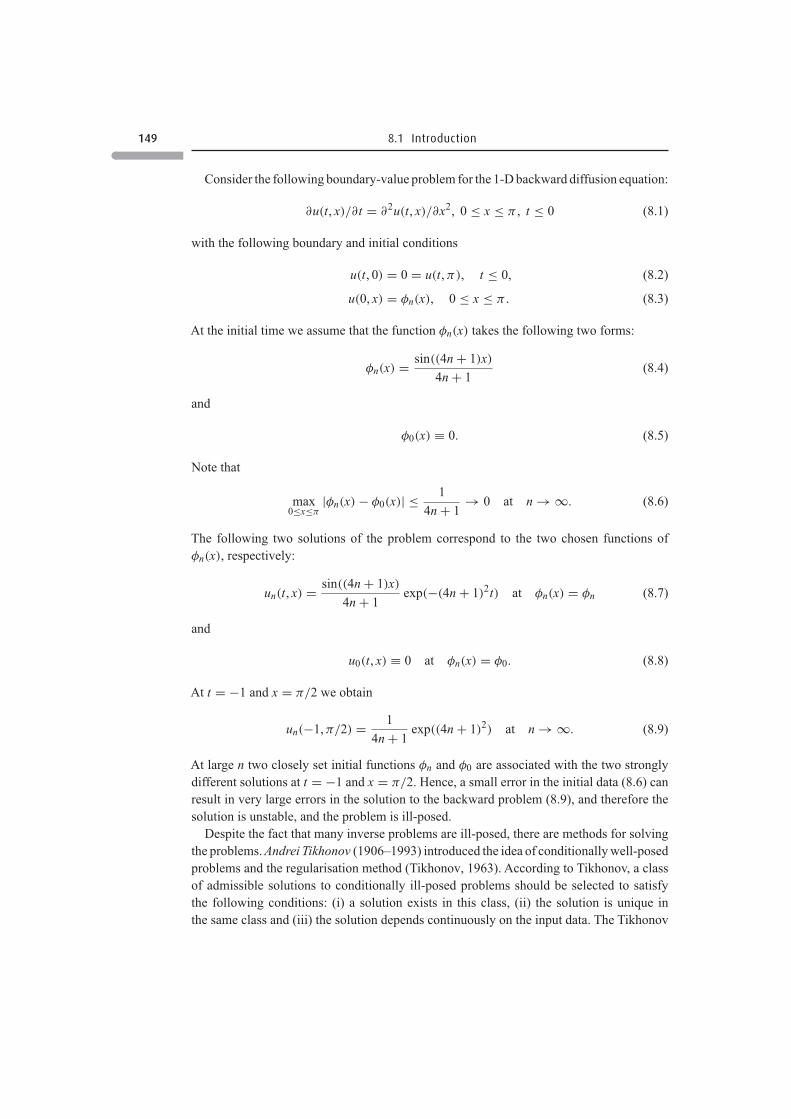
Consider the following boundary-value problem for the 1-D backward diffusion equation:
∂u(t, x)/∂t = ∂2u(t, x)/∂x2, 0 ≤ x ≤ π , t ≤ 0 (8.1)
with the following boundary and initial conditions
u(t, 0) = 0 = u(t, π), t ≤ 0, (8.2)
u(0, x) = φn(x), 0 ≤ x ≤ π . (8.3)
At the initial time we assume that the function φn(x) takes the following two forms:
φn(x) = sin((4n + 1)x)
4n + 1(8.4)
and
φ0(x) ≡ 0. (8.5)
Note that
max0≤x≤π
|φn(x) − φ0(x)| ≤ 1
4n + 1→ 0 at n → ∞. (8.6)
The following two solutions of the problem correspond to the two chosen functions ofφn(x), respectively:
un(t, x) = sin((4n + 1)x)
4n + 1exp(−(4n + 1)2t) at φn(x) = φn (8.7)
and
u0(t, x) ≡ 0 at φn(x) = φ0. (8.8)
At t = −1 and x = π/2 we obtain
un(−1, π/2) = 1
4n + 1exp((4n + 1)2) at n → ∞. (8.9)
At large n two closely set initial functions φn and φ0 are associated with the two stronglydifferent solutions at t = −1 and x = π/2. Hence, a small error in the initial data (8.6) canresult in very large errors in the solution to the backward problem (8.9), and therefore thesolution is unstable, and the problem is ill-posed.
Despite the fact that many inverse problems are ill-posed, there are methods for solvingthe problems. Andrei Tikhonov (1906–1993) introduced the idea of conditionally well-posedproblems and the regularisation method (Tikhonov, 1963). According to Tikhonov, a classof admissible solutions to conditionally ill-posed problems should be selected to satisfythe following conditions: (i) a solution exists in this class, (ii) the solution is unique inthe same class and (iii) the solution depends continuously on the input data. The Tikhonov
150 Data assimilation methods
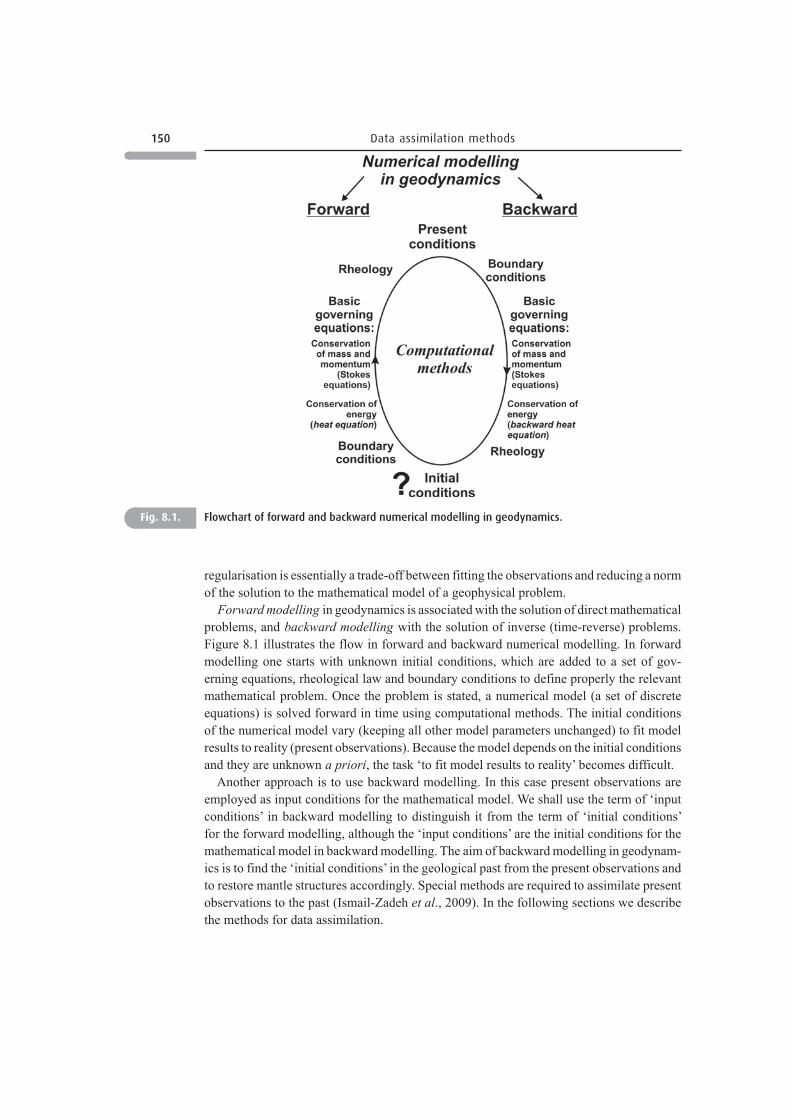
Fig. 8.1. Flowchart of forward and backward numerical modelling in geodynamics.
regularisation is essentially a trade-off between fitting the observations and reducing a normof the solution to the mathematical model of a geophysical problem.
Forward modelling in geodynamics is associated with the solution of direct mathematicalproblems, and backward modelling with the solution of inverse (time-reverse) problems.Figure 8.1 illustrates the flow in forward and backward numerical modelling. In forwardmodelling one starts with unknown initial conditions, which are added to a set of gov-erning equations, rheological law and boundary conditions to define properly the relevantmathematical problem. Once the problem is stated, a numerical model (a set of discreteequations) is solved forward in time using computational methods. The initial conditionsof the numerical model vary (keeping all other model parameters unchanged) to fit modelresults to reality (present observations). Because the model depends on the initial conditionsand they are unknown a priori, the task ‘to fit model results to reality’ becomes difficult.
Another approach is to use backward modelling. In this case present observations areemployed as input conditions for the mathematical model. We shall use the term of ‘inputconditions’ in backward modelling to distinguish it from the term of ‘initial conditions’for the forward modelling, although the ‘input conditions’ are the initial conditions for themathematical model in backward modelling. The aim of backward modelling in geodynam-ics is to find the ‘initial conditions’ in the geological past from the present observations andto restore mantle structures accordingly. Special methods are required to assimilate presentobservations to the past (Ismail-Zadeh et al., 2009). In the following sections we describethe methods for data assimilation.
151 8.2 Data assimilation
8.2 Data assimilation
The mantle is heated from the core and from inside owing to decay of radioactive elements.Since thermal convection in the mantle is described by heat advection and diffusion, one canask: is it possible to tell, from the present temperature distribution estimations of the Earth,something about the Earth’s temperature distribution in the geological past? Even thoughheat diffusion is irreversible in the physical sense, it is possible to predict accurately theheat transfer backwards in time by using data assimilation techniques without contradictingthe basic thermodynamic laws (see, for example, Ismail-Zadeh et al., 2004a, 2007).
To restore mantle dynamics in the geological past, data assimilation techniques can beused to constrain the initial conditions for the mantle temperature and velocity from theirpresent observations. The initial conditions so obtained can then be used to run forwardmodels of mantle dynamics to restore the evolution of mantle structures. Data assimilationcan be defined as the incorporation of observations (in the present) and initial conditions(in the past) in an explicit dynamic model to provide time continuity and coupling amongthe physical fields (e.g. velocity, temperature). The basic principle of data assimilationis to consider the initial condition as a control variable and to optimise the initial con-dition in order to minimise the discrepancy between the observations and the solutionof the model.
If heat diffusion is neglected, the present mantle temperature and flow can be assimilatedinto the past by using the backward advection (BAD). Numerical approaches to the solutionof the inverse problem of the Rayleigh–Taylor instability were developed for a dynamicrestoration of diapiric structures to their earlier stages (Ismail-Zadeh et al., 2001b; Kausand Podladchikov, 2001; Korotkii et al., 2002; Ismail-Zadeh et al., 2004b). Steinberger andO’Connell (1998) and Conrad and Gurnis (2003) modelled the mantle flow backwards intime from present-day mantle density heterogeneities inferred from seismic observations.
In sequential filtering a numerical model is computed forward in time for the interval forwhich observations have been made, updating the model each time where observations areavailable. The sequential filtering was used to compute mantle circulation models (Bungeet al., 1998, 2002). Despite sequential data assimilation well adapted to mantle circulationstudies, each individual observation influences the model state at later times. Informationpropagates from the geological past into the future, although our knowledge of the Earth’smantle at earlier times is much poorer than that at present.
The variational (VAR) data assimilation method has been pioneered by meteorologistsand used very successfully to improve operational weather forecasts (see Kalnay, 2003).The data assimilation has also been widely used in oceanography (see Bennett, 1992) and inhydrological studies (see McLaughlin, 2002). The use of VAR data assimilation in modelsof mantle dynamics (to estimate mantle temperature and flow in the geological past) hasbeen put forward by Bunge et al. (2003) and Ismail-Zadeh et al. (2003a, b) independently.The major differences between the two approaches are that Bunge et al. (2003) applied theVAR method to the coupled Stokes, continuity and heat equations (generalised inverse),whereas Ismail-Zadeh et al. (2003a) applied the VAR method to the heat equation only. TheVAR approach by Ismail-Zadeh et al. (2003a) is computationally less expensive, because
152 Data assimilation methods
it does not involve the Stokes equation in the iterations between the direct and adjointproblems. Moreover, this approach admits the use of temperature-dependent viscosity.
The VAR data assimilation algorithm was employed for numerical restoration of modelsof present prominent mantle plumes to their past stages (Ismail-Zadeh et al., 2004a; Hier-Majumder et al., 2005). Effects of thermal diffusion and temperature-dependent viscosityon the evolution of mantle plumes was studied by Ismail-Zadeh et al. (2006) to recoverthe structure of mantle plumes prominent in the past from that of present plumes weakenedby thermal diffusion. Liu and Gurnis (2008) simultaneously inverted mantle propertiesand initial conditions using the VAR data assimilation method and applied the method toreconstruct the evolution of the Farallon Plate subduction (Liu et al., 2008).
The quasi-reversibility (QRV) method was introduced by Lattes and Lions (1969). Theuse of the QRV method implies the introduction into the backward heat equation of theadditional term involving the product of a small regularisation parameter and a higher-order temperature derivative. The data assimilation in this case is based on a search of thebest fit between the forecast model state and the observations by minimising the regularisa-tion parameter. The QRV method was introduced in geodynamic modelling (Ismail-Zadehet al., 2007) and employed to assimilate data in models of mantle dynamics (Ismail-Zadehet al., 2008).
In this chapter we describe three principal techniques used to assimilate data relatedto geodynamics: (i) backward advection, (ii) variational (adjoint) and (iii) quasi-reversibility methods.
8.3 Backward advection (BAD) method
We consider the three-dimensional model domain � = [0, x1 = 3h] × [0, x2 = 3h] ×[0, x3 = h], where x = (x1, x2, x3) are the Cartesian coordinates and h is the depth of thedomain, and assume that the mantle behaves as a Newtonian incompressible fluid with atemperature-dependent viscosity and infinite Prandtl number. The mantle flow is describedby heat, motion and continuity equations (Chandrasekhar, 1961). To simplify the governingequations, we make the Boussinesq approximation (Boussinesq, 1903) keeping the densityconstant everywhere except for buoyancy term in the equation of motion. In the Boussinesqapproximation the dimensionless equations take the form:
∂T/∂t + u · ∇T = ∇2T , x ∈ �, t ∈ (0, ϑ), (8.10)
∇P = div [ηE] + RaTe, E = {∂ui/∂xj + ∂uj/∂xi}, e = (0, 0, 1), (8.11)
divu = 0, t ∈ (0, ϑ), x ∈ �. (8.12)
Here T , t, u = (u1, u2, u3), P and η are dimensionless temperature, time, velocity, pressureand viscosity, respectively. The Rayleigh number is defined as Ra = αgρref Th3η−1
ref κ−1,
where α is the thermal expansivity, g is the acceleration due to gravity, ρref and ηref are thereference typical density and viscosity, respectively; T is the temperature contrast between
153 8.4 Application of the BAD method
the lower and upper boundaries of the model domain; and κis the thermal diffusivity. In Eqs.(8.10)–(8.12) length, temperature and time are normalised by h,T and h2κ−1, respectively.
At the boundary � of the model domain � we set the impenetrability condition withno-slip or perfect slip conditions: u = 0 or ∂uτ /∂n = 0, u · n = 0, where n is the outwardunit normal vector at a point on the model boundary, and uτ is the projection of the velocityvector onto the tangent plane at the same point on the model boundary. We assume zeroheat flux through the vertical boundaries of the box. Either temperature or heat flux areprescribed at the upper and lower boundaries of the model domain. To solve the problemforward or backward in time we assume the temperature to be known at the initial time(t = 0) or at the present time (t = ϑ). Equations (8.10)–(8.12) together with the boundaryand initial conditions describe a thermo-convective mantle flow.
The principal difficulty in solving the problem (8.10)–(8.12) backward in time is theill-posedness of the backward heat problem and the presence of the heat diffusion termin the heat equation. The backward advection (BAD) method suggests neglecting the heatdiffusion term, and the heat advection equation can then be solved backward in time. Bothdirect (forward in time) and inverse (backward in time) problems of the heat (density)advection are well-posed. This is because the time-dependent advection equation has thesame form of characteristics for the direct and inverse velocity field (the vector velocityreverses its direction, when time is reversed). Therefore, numerical algorithms used tosolve the direct problem of the gravitational instability can also be used in studies of thetime-reverse problems by replacing positive time steps with negative ones.
Using the BAD method, Steinberger and O’Connell (1998) studied the motion of hotspotsrelative to the deep mantle. They combined the advection of plumes, which are thought tocause the hotspots on the Earth’s surface, with a large-scale mantle flow field and constrainedthe viscosity structure of the Earth’s mantle. Conrad and Gurnis (2003) modelled the historyof mantle flow by using a tomographic image of the mantle beneath southern Africa asan input (initial) condition for the backward mantle advection model while reversing thedirection of flow. If the resulting model of the evolution of thermal structures obtained bythe BAD method is used as a starting point for a forward mantle convection model, presentmantle structures can be reconstructed if the time of assimilation does not exceed 50–75 Myr.
8.4 Application of the BAD method: restoration of theevolution of salt diapirs
Salt is so buoyant and weak compared with most other rocks with which it is found that itdevelops distinctive structures with a wide variety of shapes and relationships with otherrocks by various combinations of gravity, thermal effects and lateral forces. The crests ofpassive salt bodies can stay near the sedimentation surface while their surroundings areburied (downbuilt) by other sedimentary rocks (Jackson et al., 1994). The profiles of down-built passive diapirs can simulate those of fir trees because they reflect the ratio of increasein diapir height relative to the rate of accumulation of the downbuilding sediments (Talbot,1995) and lateral forces (Koyi, 1996). Salt movements can be triggered by faulting and
154 Data assimilation methods
driven by erosion and redeposition, differential loading, buoyancy and other geologicalprocesses. Many salt sequences are buried by overburdens sufficiently stiff to resist thebuoyancy of the salt. Such salt will only be driven by differential loading into sharp-crestedreactive-diapiric walls after the stiff overburden is weakened and thinned by faults (Vendev-ille and Jackson, 1992). Such reactive diapirs often rise up and out of the fault zone andthereafter can continue increasing in relief as by passive downbuilding of more sediment.
Active diapirs are those that lift or displace their overburdens. Although any erosion ofthe crests of salt structures and deposition of surrounding overburden rocks influence theirgrowth, diapirs with significant relief have sufficient buoyancy to rise (upbuild) throughstiff overburdens (Jackson et al., 1994). The rapid deposition of denser and more viscoussediments over less dense and viscous salt results in the Rayleigh–Taylor instability. Thisleads to a gravity-driven single overturn of the salt layer with its denser but ductile overbur-den. Rayleigh–Taylor overturns (Ramberg, 1968) are characterised by the rise of rocksaltthrough overlying and younger compacting clastic sediments that are deformed as a result.The consequent salt structures evolve through a great variety of shapes. Perturbations ofthe interface between salt and its denser overburden result in the overburden subsiding assalt rises owing to the density inversion.
Two-dimensional (2-D) numerical models of salt diapirism were first developed by Woidt(1978) who examined how the viscosity ratio between the salt and its overburden affectsthe shapes and growth rate of diapirs. Schmeling (1987) demonstrated how the dominantwavelength and the geometry of gravity overturns are influenced by the initial shape ofthe interface between the salt and its overburden. Römer and Neugebauer (1991) presentednumerical results of modelling diapiric structures in a multilayered medium. Later Poliakovet al. (1993a) and Naimark et al. (1998) developed numerical models of diapiric growthconsidering the effects of sedimentation and redistribution of sediments. Van Keken et al.(1993), Poliakov et al. (1993b), Daudre and Cloetingh (1994), and Poliakov et al. (1996)introduced non-linear rheological properties of salt and overburden into their numericalmodels. The authors mentioned above used various numerical methods to compute themodels of salt diapirism, among them FD method, Lagrangian and Eulerian FE method andtheir combination.
Two-dimensional analyses of the evolution of salt structures are restricted and not suitablefor examining the complicated shapes of mature diapiric patterns. Resolving the geometryof gravity overturns requires three-dimensional (3-D) numerical modelling. Ismail-Zadehet al. (2000b) analysed such typical 3-D structures as deep polygonal buoyant ridges, shallowsalt-stock canopies and salt walls. Kaus and Podladchikov (2001) showed how complicated3-D diapirs developed from initial 2-D perturbations of the interface between salt andits overburden.
The increasing application of 3-D seismic exploration in oil and gas prospecting points tothe need for vigorous efforts toward numerical modelling of the evolution of salt structuresin three dimensions, both forward and backward in time. Most numerical models of saltdiapirism involved the forward evolution of salt structures toward increasing maturity.Ismail-Zadeh et al. (2001b) developed a numerical approach to 2-D dynamic restorationof cross-sections across salt structures. The approach was based on solving the inverseproblem of gravitational instability by the BAD method. The same method was used in
155 8.4 Application of the BAD method
3-D cases to model Rayleigh-Taylor instability backward in time (Kaus and Podladchikov,2001; Korotkii et al., 2002; Ismail-Zadeh et al., 2004b).
We consider here the advection problem (slow flow of an incompressible fluid of variabledensity and viscosity due to gravity) in the rectangular domain �. A 3-D model of the flowof salt and of the viscous deformation of the overburden of salt is described by the Stokesequations (8.11), where the term Ra T is replaced by the term −gρ, and by Eq. (8.10), wheretemperature T is replaced by density ρ (viscosity η) and the term on the right-hand side isomitted. Equation (8.10) in this case describes the advection of density (viscosity) with theflow. For details of the numerical model see Section 4.10.2.
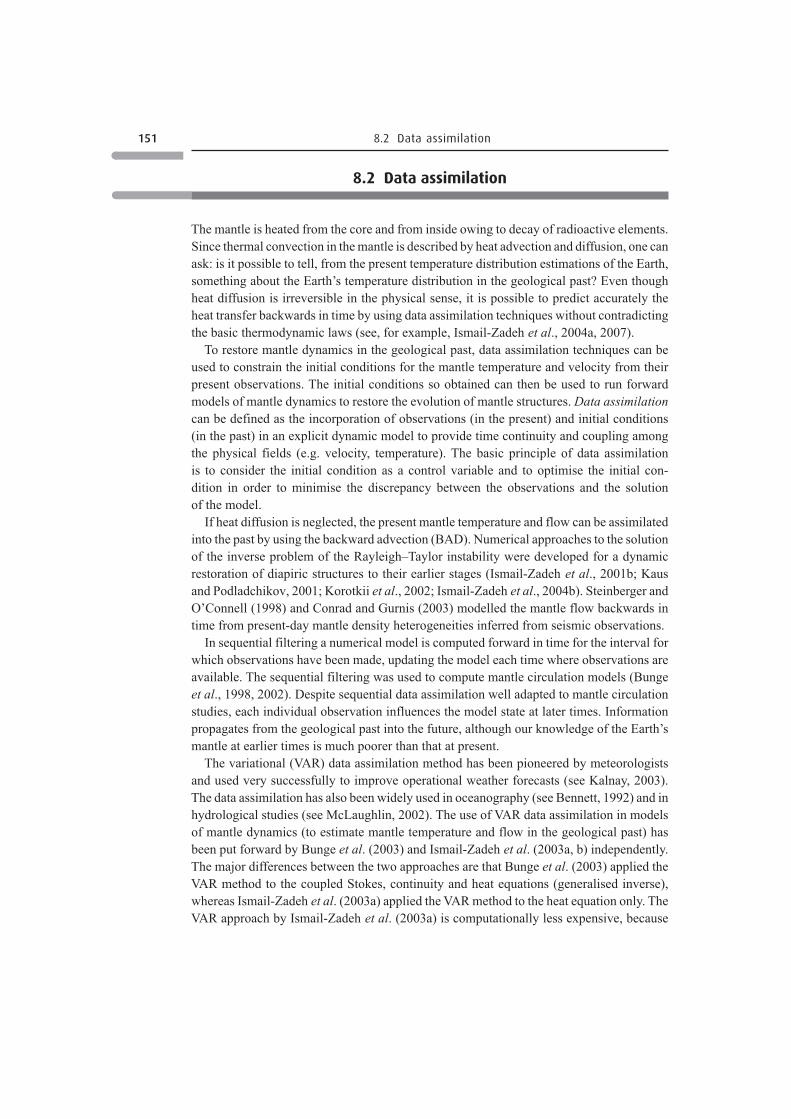
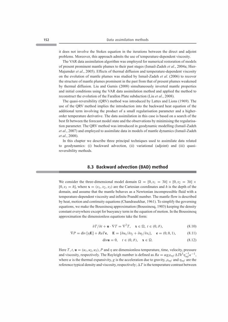
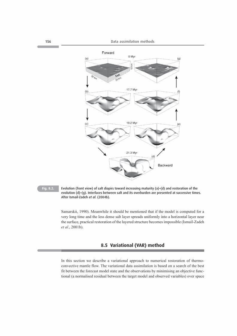
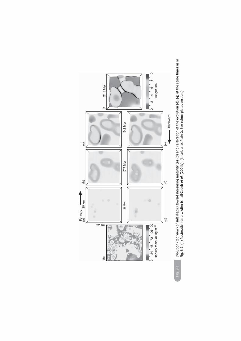
Although dimensionless values and functions are used in computations, numerical resultsare presented in dimensional form for the reader’s convenience. The time step t is chosenfrom the condition that the maximum displacement does not exceed a given small valueh: t = h/umax, where umax is the maximum value of the flow velocity. Salt diapirs inthe numerical model evolve from random initial perturbations of the interface between thesalt and its overburden deposited on the top of horizontal salt layer prior to the interfaceperturbation. Initially the evolution of salt diapirs is modelled forward in time as presentedin the model example in Section 4.10.2. Figures 8.2 (a–d, a front view) and 8.3 (a–d, atop view) show the positions of the interface between salt and overburden in the model atsuccessive times over a period of about 21 Myr.
To restore the evolution of salt diapirs predicted by the forward model through successiveearlier stages, a positive time is replaced by a negative time, and the problem is solved back-ward in time. Such a replacement is possible, because the characteristics of the advectionequations have the same form for both direct and inverse velocity fields. The final positionof the interface between salt and its overburden in the forward model (Figs. 8.2d and 8.3d)is used as an initial position of the interfaces for the backward model. Figures 8.2, d–g and8.3, d–g illustrate successive steps in the restoration of the upbuilt diapirs. Least squareerrors δ of the restoration are calculated by using the formula:
δ(x1, x2) =⎛⎝
h∫0
(ρ(x1, x2, x3) − ρ̃(x1, x2, x3))2 dx3
⎞⎠
1/2
, (8.13)
where ρ(x1, x2, x3) is the density at initial time, and ρ̃(x1, x2, x3) is the restored density(Fig. 8.3h). The maximum value δ does not exceed 120 kg m−3, and the error is associatedwith small areas of the initial interface’s perturbation.
To demonstrate the stability of the restoration results with respect to changes in the densityof the overburden, the restoration procedure was tested by synthetic examples. Initially theforward model is run for 200 computational time steps (about 30 Myr). Then the densitycontrast (δρ) between salt and its overburden is changed by a few per cent: namely, δρ
was chosen to be 400, 405, 410 (the actual contrast), 415 and 420 kg m−3. The evolutionof the system was restored for these density contrasts. Ismail-Zadeh et al. (2004b) foundsmall discrepancies (less than 0.5%) between least square errors for all these test cases.The tests show that the solution is stable to small changes in the initial conditions, andthis is in agreement with the mathematical theory of well-posed problems (Tikhonov and
156 Data assimilation methods
(a)
(b)
(c)
(d)
(e)
(f)
(g)0 Myr
17.7 Myr
19.2 Myr
21.3 Myr
Fig. 8.2. Evolution (front view) of salt diapirs toward increasing maturity (a)–(d) and restoration of theevolution (d)–(g). Interfaces between salt and its overburden are presented at successive times.After Ismail-Zadeh et al. (2004b).
Samarskii, 1990). Meanwhile it should be mentioned that if the model is computed for avery long time and the less dense salt layer spreads uniformly into a horizontal layer nearthe surface, practical restoration of the layered structure becomes impossible (Ismail-Zadehet al., 2001b).
8.5 Variational (VAR) method
In this section we describe a variational approach to numerical restoration of thermo-convective mantle flow. The variational data assimilation is based on a search of the bestfit between the forecast model state and the observations by minimising an objective func-tional (a normalised residual between the target model and observed variables) over space
For
war
d
0 M
yr17
.7 M
yr19
.2 M
yr
21.3
Myr
(a)
(b)
30 k
m
30 km
(c)
(d)
(e)
(f)
(g)
024
48D
ensi
ty r
esid
ual,
kg m
–372
9612
00
24
Hei
ght,
km
Bac
kwar
d
68
10
(h)
Fig.8.3.
Evolution(topview)ofsaltdiapirstowardincreasingmaturity(a)–(d)andrestorationoftheevolution(d)–(g)atthesametimesasin
Fig.8.2.(h)Restorationerrors.AfterIsmail-Zadehet
al.(2004b).(IncolourasPlate2.Seecolourplatessection.)
158 Data assimilation methods
and time. To minimise the objective functional over time, an assimilation time interval isdefined and an adjoint model is typically used to find the derivatives of the objective func-tional with respect to the model states. The variational data assimilation is well suited forsmooth problems (we discuss the problem of smoothness in Section 8.7).
The method for variational data assimilation can be formulated with a weak constraint (ageneralised inverse) where errors in the model formulation are taken into account (Bungeet al., 2003) or with a strong constraint where the model is assumed to be perfect except forthe errors associated with the initial conditions (Ismail-Zadeh et al., 2003a). Actually thereare several sources of errors in forward and backward modelling of thermo-convective man-tle flow, which we discuss in Section 8.12. The generalised inverse of mantle convectionconsiders model errors, data misfit and the misfit of parameters as control variables. Unfortu-nately the generalised inverse presents a tremendous computational challenge and is difficultto solve in practice. Hence, Bunge et al. (2003) considered a simplified generalised inverseimposing a strong constraint on errors (ignoring all errors except for the initial conditionerrors). Therefore, the strong constraint makes the problem computationally tractable.
We consider the following objective functional at t ∈ [0, ϑ]
J (ϕ) = ‖T (ϑ , ·; ϕ) − χ(·)‖2 , (8.14)
where ‖ · ‖ denotes the norm in the space L2(�) (the Hilbert space with the norm defined as‖y‖ = [∫
�y2(x)dx]1/2). Since in what follows the dependence of solutions of the thermal
boundary value problems on initial data is important, we introduce these data explicitlyinto the mathematical representation of temperature. Here T (ϑ , ·; ϕ) is the solution of thethermal boundary value problem (8.10) at the final time ϑ , which corresponds to some(unknown as yet) initial temperature distribution ϕ(x); χ(x) = T (ϑ , x; T0) is the knowntemperature distribution at the final time, which corresponds to the initial temperature T0(·).The functional has its unique global minimum at value ϕ ≡ T0 and J (T0) ≡ 0, ∇J (T0) ≡ 0(Vasiliev, 2002).
To find the minimum of the functional we employ the gradient method (k = 0, . . . , j, . . .):
ϕk+1 = ϕk − βk∇J (ϕk), ϕ0 = T∗, (8.15)
βk ={
J (ϕk)/ ‖∇J (ϕk)‖ , 1 ≤ k ≤ k∗1/(k + 1), k > k∗
, (8.16)
where T∗ is an initial temperature guess. The minimisation method belongs to a class oflimited-memory quasi-Newton methods (Zou et al., 1993), where approximations to theinverse Hessian matrices are chosen to be the identity matrix. Equation (8.16) is usedto maintain the stability of the iteration scheme (8.15). Consider that the gradient of theobjective functional ∇J (ϕk) is computed with an error ‖∇Jδ(ϕk) − ∇J (ϕk)‖ < δ, where∇Jδ(ϕk) is the computed value of the gradient. We introduce the function ϕ∞ = ϕ0 −∑∞
k=1 βk∇J (ϕk), assuming that the infinite sum exists, and the function ϕ∞δ = ϕ0 −∑∞
k=1 βk∇J (δ ϕk) as the computed value of ϕ∞. For stability of the iteration method (8.15),
159 8.5 Variational (VAR) method
the following inequality should be held:
∥∥ϕ∞δ − ϕ∞∥∥ =
∥∥∥∥∥∞∑
k=1
βk(∇Jδ(uk) − ∇J (uk))
∥∥∥∥∥
≤∞∑
k=1
βk ‖∇Jδ(ϕk) − ∇J (ϕk)‖ ≤ δ
∞∑k=1
βk .
The sum∑∞
k=1 βk is finite, ifβk = 1/kp, p > 1.We use p = 1, but the number of iterations islimited, and therefore, the iteration method is conditionally stable, although the convergencerate of these iterations is low. Meanwhile the gradient of the objective functional ∇J (ϕk)
decreases steadily with the number of iterations providing the convergence, although theabsolute value of J (ϕk)/‖∇J (ϕk)‖ increases with the number of iterations, and it can resultin instability of the iteration process (Samarskii and Vabischevich, 2004).
The minimisation algorithm requires the calculation of the gradient of the objectivefunctional, ∇J . This can be done through the use of the adjoint problem for the modelequations (8.10)–(8.12) with the relevant boundary and initial conditions. In the case of theheat problem, the adjoint problem can be represented in the following form:
∂�/∂t + u · ∇� + ∇2� = 0, x ∈ �, t ∈ (0, ϑ),
σ1� + σ2∂�/∂n = 0, x ∈ �, t ∈ (0, ϑ),
�(ϑ , x) = 2(T (ϑ , x; ϕ) − χ(x)), x ∈ �, (8.17)
where σ1 and σ2 are some smooth functions or constants satisfying the condition σ 21 +σ 2
2 =0. Selecting σ1 and σ2 we can obtain corresponding boundary conditions.
The solution to the adjoint problem (8.17) is the gradient of the objective functional (8.14).To prove the statement, we consider an increment of the functional J in the following form:
J (ϕ + h) − J (ϕ) =∫�
(T (ϑ , x; ϕ + h) − χ(x))2 dx −∫�
(T (ϑ , x; ϕ) − χ(x))2 dx
= 2∫�
(T (ϑ , x; ϕ) − χ(x)) ζ(ϑ , x)dx +∫�
ζ 2(ϑ , x)dx
=∫�
�(ϑ , x)ζ(ϑ , x)dx +∫�
ζ 2(ϑ , x)dx
=∫�
ϑ∫0
∂
∂t(�(t, x)ζ(t, x)) dxdt +
∫�
�(0, x)h(x)dx +∫�
ζ 2(ϑ , x)dx,
(8.18)
where �(t, x) = 2(T (t, x; ϑ) − χ(x)); h(x) is a small heat increment to the unknown initialtemperature ϕ(x); and ζ = T (t, x; ϕ+h)−T (t, x; ϕ) is the solution to the following forward
160 Data assimilation methods
heat problem
∂ζ/∂t + u · ∇ζ − ∇2ζ = 0, x ∈ �, t ∈ (0, ϑ),
σ1ζ + σ2∂ζ/∂n = 0, x ∈ �, t ∈ (0, ϑ),
ζ(0, x) = h(x), x ∈ �. (8.19)
Considering the fact that � = �(t, x) and ζ = ζ(t, x) are the solutions to (8.17) and (8.19)respectively, and the velocity u satisfies (8.12) and the boundary conditions specified,we obtain
∫�
ϑ∫0
∂
∂t(�(t, x)ζ(t, x)) dtdx =
ϑ∫0
∫�
{∂
∂t�(t, x)ζ(t, x) + �(t, x)
∂ζ(t, x)
∂t
}dxdt
=ϑ∫
0
∫�
ζ(t, x)[−u · ∇� − ∇2�
]dxdt +
ϑ∫0
∫�
�(t, x)[−u · ∇ζ + ∇2ζ
]dxdt
=ϑ∫
0
∫�
{�∇ζ · n − ζ∇� · n}d�dt +ϑ∫
0
∫�
{∇� · ∇ζ − ∇ζ · ∇�}dxdt
+ϑ∫
0
∫�
{ζ�∇ · u + �u · ∇ζ − �u · ∇ζ } dxdt − 2
ϑ∫0
∫�
ζ�u · n d�dt = 0.
(8.20)
Hence
J (ϕ + h) − J (ϕ) =∫�
�(0, x)h(x)dx+∫�
ζ 2(ϑ , x)dx =∫�
�(0, x)h(x)dx + o(‖h‖).
(8.21)
The gradient is derived by using the Gateaux derivative of the objective functional.Therefore, we obtain that the gradient of the functional is represented as
∇J (ϕ) = �(0, ·). (8.22)
Thus, the solution of the backward heat problem is reduced to solutions of series of for-ward problems, which are known to be well-posed (Tikhonov and Samarskii, 1990). Thealgorithm can be used to solve the problem over any subinterval of time in [0, ϑ].
We note that information on the properties of the Hessian matrix (∇2J ) is important inmany aspects of minimisation problems (Daescu and Navon, 2003). To obtain sufficientconditions for the existence of the minimum of the problem, the Hessian matrix must bepositive definite at T0 (optimal initial temperature). However, an explicit evaluation of theHessian matrix in many cases is prohibitive owing to the number of variables.
161 8.6 Variational (VAR) method
We now describe the algorithm for numerical solution of the inverse problem of mantleconvection, that is, the numerical algorithm to solve (8.10)–(8.12) backward in time usingthe VAR method. A uniform partition of the time axis is defined at points tn = ϑ − δt n,where δt is the time step, and n successively takes integer values from 0 to some naturalnumber m = ϑ/δt. At each subinterval of time [tn+1, tn], the search of the temperature Tand flow velocity u at t = tn+1 consists of the following basic steps.
Step 1. Given the temperature T = T (tn, x) at t = tn solve a set of linear algebraic equationsderived from (8.11) and (8.12) with the appropriate boundary conditions in orderto determine the velocity u.
Step 2. The ‘advective’ temperature Tadv = Tadv(tn+1, x) is determined by solving theadvection heat equation backward in time, neglecting the diffusion term in Eq.(8.10). This can be done by replacing positive time steps by negative ones (seeSection 8.4). Given the temperature T = Tadv at t = tn+1 steps 1 and 2 are thenrepeated to find the velocity uadv = u(tn+1, x; Tadv).
Step 3. The heat equation (8.10) is solved with appropriate boundary conditions and initialcondition ϕk(x) = Tadv(tn+1, x), k = 0, 1, 2, . . . , m, . . . forward in time usingvelocity uadv in order to find T (tn, x; ϕk).
Step 4. The adjoint equation of (8.17) is then solved backward in time with appropriateboundary conditions and initial condition �(tn, x) = 2(T (tn, x; ϕk) − χ(x)) usingvelocity u in order to determine ∇J (ϕk) = �(tn+1, x; ϕk).
Step 5. The coefficient βk is determined from (8.16), and the temperature is updated (i.e.ϕk+1 is determined) from (8.15).
Steps 3 to 5 are repeated until
δϕn = J (ϕn) + ‖∇J (ϕn)‖2 < ε, (8.23)
where ε is a small constant. Temperature ϕk is then considered to be the approximation tothe target value of the initial temperature T (tn+1, x). And finally, step 1 is used to determinethe flow velocity u(tn+1, x; T (tn+1, x)). Step 2 introduces a pre-conditioner to acceleratethe convergence of temperature iterations in steps 3 to 5 at high Rayleigh number. Atlow Ra, step 2 is omitted and uadv is replaced by u. After these algorithmic steps, weobtain temperature T = T (tn, x) and flow velocity u = u(tn, x) corresponding to t = tn,n = 0, . . . , m. Based on the obtained results, we can use interpolation to reconstruct, whenrequired, the entire process on the time interval [0, ϑ] in more detail.
Thus, at each subinterval of time we apply the VAR method to the heat equation only,iterate the direct and conjugate problems for the heat equation in order to find temperature,and determine backward flow from the Stokes and continuity equations twice (for ‘advec-tive’ and ‘true’ temperatures). Compared to the VAR approach by Bunge et al. (2003),the described numerical approach is computationally less expensive, because we do notinvolve the Stokes equation in the iterations between the direct and conjugate problems(the numerical solution of the Stokes equation is the most time consuming calculation).
162 Data assimilation methods
8.6 Application of the VAR method: restoration ofmantle plume evolution
A plume is hot, narrow mantle upwelling that is invoked to explain hotspot volcanism. Ina temperature-dependent viscosity fluid such as the mantle, a plume is characterised by amushroom-shaped head and a thin tail. Upon impinging under a moving lithosphere, such amantle upwelling should therefore produce a large amount of melt and successive massiveeruption, followed by smaller but long-lived hot-spot activity fed from the plume tail (Mor-gan, 1972; Richards et al., 1989; Sleep, 1990). Meanwhile, slowly rising plumes (a buoyancyflux of less than 103 kg s−1) coming from the core–mantle boundary should have cooledso much that they would not melt beneath old lithosphere (Albers and Christensen, 1996).
Mantle plumes evolve in three distinguishing stages: (i) immature, i.e. an origin andinitial rise of the plumes; (ii) mature, i.e. plume–lithosphere interaction, gravity spread-ing of plume head and development of overhangs beneath the bottom of the lithosphere,and partial melting of the plume material (see Ribe and Christensen, 1994; Moore et al.,1998); and (iii) overmature, i.e. slowing-down of the plume rise and fading of the man-tle plumes due to thermal diffusion (Davaille and Vatteville, 2005; Ismail-Zadeh et al.,2006). The ascent and evolution of mantle plumes depend on the properties of the sourceregion (that is, the thermal boundary layer) and the viscosity and thermal diffusivity ofthe ambient mantle. The properties of the source region determine the temperature andviscosity of the mantle plumes. Structure, flow rate and heat flux of the plumes are con-trolled by the properties of the mantle through which the plumes rise. While propertiesof the lower mantle (e.g. viscosity, thermal conductivity) are relatively constant duringabout 150 Myr lifetime of most plumes, source region properties can vary substantiallywith time as the thermal basal boundary layer feeding the plume is depleted of hot material(Schubert et al., 2001). Complete local depletion of this boundary layer cuts the plume offfrom its source.
A mantle plume is a well-established structure in computer modelling and laboratoryexperiments. Numerical experiments on dynamics of mantle plumes (Trompert and Hansen,1998a,b; Zhong, 2005) showed that the number of plumes increases and the rising plumesbecome thinner with an increase in Rayleigh number. Disconnected thermal plume struc-tures appear in thermal convection at Ra greater than 107 (Hansen et al., 1990; Malevskyet al., 1992). At high Ra (in the hard turbulence regime) thermal plumes are torn off theboundary layer by the large-scale circulation or by non-linear interactions between plumes(Malevsky and Yuen, 1993). Plume tails can also be disconnected when the plumes aretilted by plate scale flow (see Olson and Singer, 1985; Steinberger and O’Connell, 1998).Ismail-Zadeh et al. (2006) presented an alternative explanation for the disconnected mantleplume heads and tails that is based on thermal diffusion of mantle plumes.
A dimensionless temperature-dependent viscosity law (Busse et al., 1993) is employedin the models discussed in this chapter
η(T ) = exp
(M
T + G− M
0.5 + G
), (8.24)
163 8.6 Application of the VAR method
where M = [225/ln(r)] − 0.25 ln(r), G = 15/ln(r) − 0.5, and r is the viscosity ratiobetween the upper and lower boundaries of the model domain. The temperature-dependentviscosity profile has its minimum at the core–mantle boundary. A more realistic viscosityprofile (Forte and Mitrovica, 2001) will influence the evolution of mantle plumes, thoughit will not influence the restoration of the plumes.
The model domain is divided into 37 × 37 × 29 rectangular finite elements to approxi-mate the vector velocity potential by tricubic splines, and a uniform grid 112 × 112 × 88is employed for approximation of temperature, velocity and viscosity. Temperature inthe heat equation (8.10) is approximated by finite differences and determined by thesemi-Lagrangian method (see Section 7.8). A numerical solution to the Stokes and incom-pressibility equations (8.11) and (8.12) is based on the introduction of a two-componentvector velocity potential and on the application of the Eulerian finite-element method witha tricubic-spline basis for computing the potential (Section 4.9 and 4.10). Such a proce-dure results in a set of linear algebraic equations with a symmetric positive-definite bandedmatrix. We solve the set of equations by the conjugate gradient method (Section 6.3.3).
8.6.1 Forward modelling
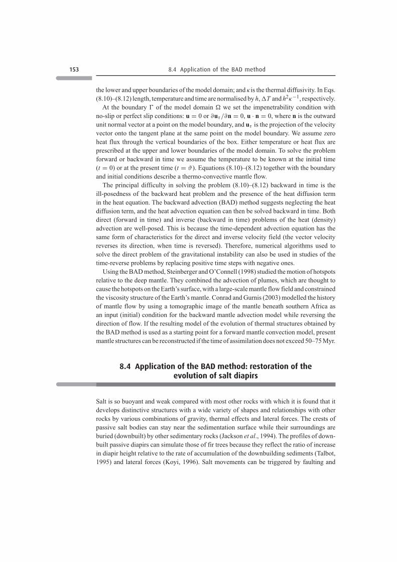
Here the evolution of mature mantle plumes is modelled initially forward in time. Withα = 3×10⁻⁵ K−1, ρref = 4000 kg m−3, T = 3000 K, h = 2800 km, ηref = 8×10²² Pa s,and κ = 10−6 m−2 s−1, the initial Rayleigh number is Ra = 9.5 × 10⁵. While plumesevolve in the convecting heterogeneous mantle, at the initial time it is assumed that theplumes develop in a laterally homogeneous temperature field, and hence the initial mantletemperature is considered to increase linearly with depth.
Mantle plumes are generated by random temperature perturbations at the top of thethermal source layer associated with the core–mantle boundary (Fig. 8.4a). The mantlematerial in the basal source layer flows horizontally toward the plumes. The reducedviscosity in this basal layer promotes the flow of the material to the plumes. Verti-cal upwelling of hot mantle material is concentrated in low viscosity conduits near thecentrelines of the emerging plumes (Fig. 8.4b,c). The plumes move upward through themodel domain, gradually forming structures with well-developed heads and tails. Coldermaterial overlying the source layer (e.g. portions of lithospheric slabs subducted to thecore–mantle boundary) replaces hot material at the locations where the source materialis fed into mantle plumes. Some time is required to recover the volume of source ma-terial depleted due to plume feeding (Howard, 1966). Because the volume of upwellingmaterial is comparable to the volume of the thermal source layer feeding the man-tle plumes, hot material could eventually be exhausted, and mantle plumes would bestarved thereafter.
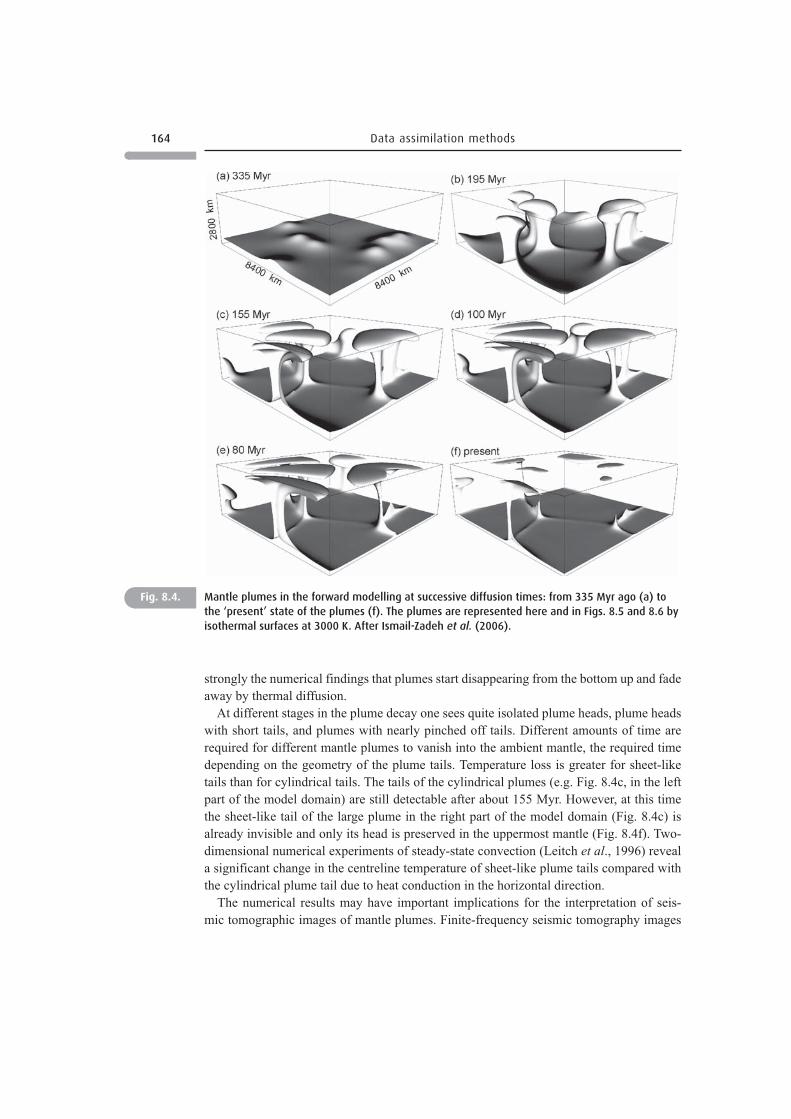
The plumes diminish in size with time (Fig. 8.4d), and the plume tails disappear beforethe plume heads (Fig. 8.4e,f). We note that Fig. 8.4 presents a hot isothermal surface of theplumes. If colder isotherms are considered, the disappearance of the isotherms will occurlater. But anyhow, hot or cold isotherms are plotted, plume tails will vanish before theirheads. Results of recent laboratory experiments (Davaille and Vatteville, 2005) support
164 Data assimilation methods
Fig. 8.4. Mantle plumes in the forward modelling at successive diffusion times: from 335 Myr ago (a) tothe ‘present’ state of the plumes (f). The plumes are represented here and in Figs. 8.5 and 8.6 byisothermal surfaces at 3000 K. After Ismail-Zadeh et al. (2006).
strongly the numerical findings that plumes start disappearing from the bottom up and fadeaway by thermal diffusion.
At different stages in the plume decay one sees quite isolated plume heads, plume headswith short tails, and plumes with nearly pinched off tails. Different amounts of time arerequired for different mantle plumes to vanish into the ambient mantle, the required timedepending on the geometry of the plume tails. Temperature loss is greater for sheet-liketails than for cylindrical tails. The tails of the cylindrical plumes (e.g. Fig. 8.4c, in the leftpart of the model domain) are still detectable after about 155 Myr. However, at this timethe sheet-like tail of the large plume in the right part of the model domain (Fig. 8.4c) isalready invisible and only its head is preserved in the uppermost mantle (Fig. 8.4f). Two-dimensional numerical experiments of steady-state convection (Leitch et al., 1996) reveala significant change in the centreline temperature of sheet-like plume tails compared withthe cylindrical plume tail due to heat conduction in the horizontal direction.
The numerical results may have important implications for the interpretation of seis-mic tomographic images of mantle plumes. Finite-frequency seismic tomography images
165 8.6 Application of the VAR method
(Montelli et al., 2004) show that a number of plumes extend to mid-mantle depths butare not visible below these depths. From a seismological point of view, the absence of theplume tails could be explained as a combination of several factors (Romanowicz and Gung,2002): elastic velocities are sensitive to composition as well as temperature; the effect oftemperature on velocities decreases with increasing pressure (Karato, 1993); and wavefronthealing effects make it difficult to accurately image low velocity bodies (Nolet and Dahlen,2000). The ‘disappearance’ of the plume tails can hence be explained as the effects of poortomographic resolution at deeper levels. Apart from this, the numerical results demonstratethe plausibility of finding a great diversity in the morphology of seismically imaged mantleplumes, including plume heads without tails and plumes with tails that are detached fromtheir sources.
8.6.2 Backward modelling
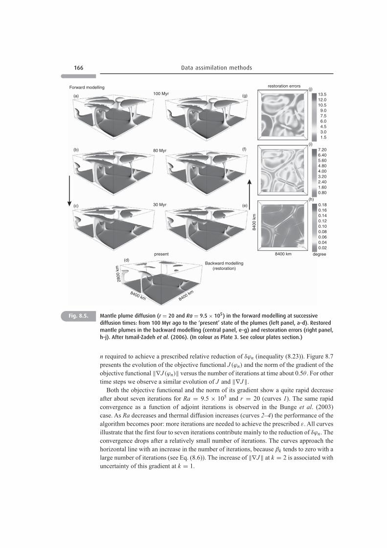
To restore the prominent state of the plumes (Fig. 8.4d) in the past from their ‘present’weakstate (Fig. 8.4f), the VAR method can be employed. Figure 8.5 illustrates the restored statesof the plumes (middle panel) and the temperature residuals δT (right panel) between thetemperature T (x) predicted by the forward model and the temperature T̃ (x) reconstructedto the same age:
δT (x1, x2) =⎡⎣
h∫0
(T (x1, x2, x3) − T̃ (x1, x2, x3)
)2dx3
⎤⎦
1/2
. (8.25)
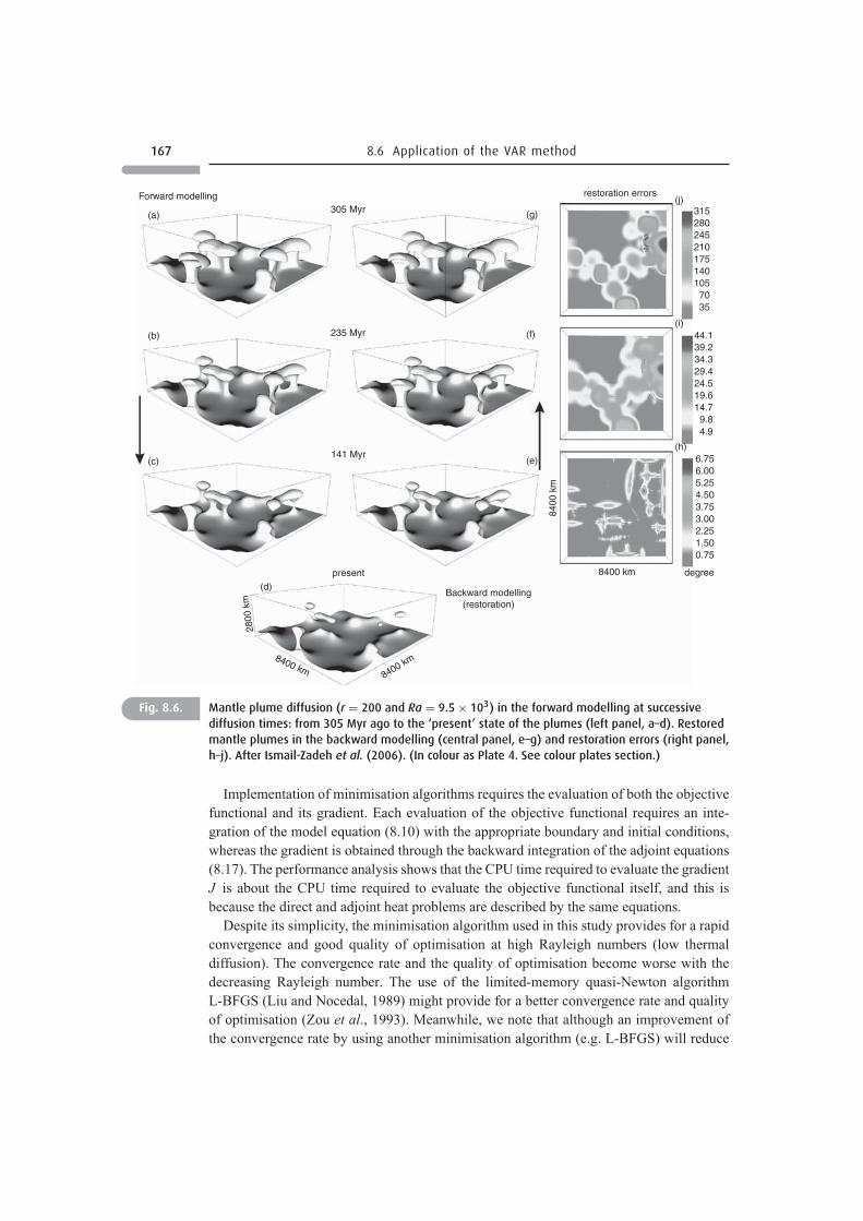
To study the effect of thermal diffusion on the restoration of mantle plumes, several exper-iments on mantle plume restoration were run for various Rayleigh number Ra (typicallyless than the initial Ra) and viscosity ratio r. Figure 8.6 presents the case of r = 200 andRa = 9.5 × 10³ and shows several stages in the diffusive decay of the mantle plumes.
The dimensional temperature residuals are within a few degrees for the initial restorationperiod (Figs. 8.5i and 8.6h). The computations show that the errors (temperature residuals)get larger the farther the restorations move backward in time (e.g. δT ≈ 300 K at therestoration time of more than 300 Myr, r = 200, and Ra = 9.5 × 10³). Compared withthe case of Ra = 9.5 × 10⁵, one can see that the residuals become larger as the Rayleighnumber decreases or thermal diffusion increases and viscosity ratio increases.
The quality of the restoration depends on the dimensionless Péclet number Pe =humaxκ
−1, where umax is the maximum flow velocity. According to the numerical experi-ments, the Péclet number corresponding to the temperature residual δT = 600 K is Pe = 10;Pe should not be less than about 10 for a high quality plume restoration.
8.6.3 Performance of the numerical algorithm
Here we analyse the performance of the VAR data assimilation algorithm for various Raand r. The performance of the algorithm is evaluated in terms of the number of iterations
166 Data assimilation methods
Forward modelling
100 Myr
restoration errors
(a)
(b)
(c)
(d)
(e)
(f)
(g)
(j)
(i)
(h)
present
Backward modelling(restoration)
8400 km 8400 km
80 Myr
30 Myr
2800
km
8400 km degree84
00 k
m
13.512.010.59.07.56.04.53.01.5
7.206.405.604.804.003.202.401.600.80
0.180.160.140.120.100.080.060.040.02
Fig. 8.5. Mantle plume diffusion (r = 20 and Ra = 9.5× 10⁵) in the forward modelling at successivediffusion times: from 100 Myr ago to the ‘present’ state of the plumes (left panel, a–d). Restoredmantle plumes in the backward modelling (central panel, e–g) and restoration errors (right panel,h–j). After Ismail-Zadeh et al. (2006). (In colour as Plate 3. See colour plates section.)
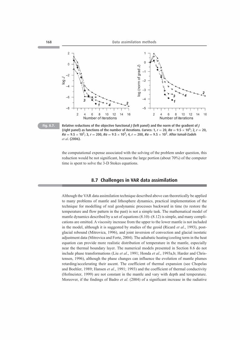
n required to achieve a prescribed relative reduction of δϕn (inequality (8.23)). Figure 8.7presents the evolution of the objective functional J (ϕn) and the norm of the gradient of theobjective functional ‖∇J (ϕn)‖ versus the number of iterations at time about 0.5θ . For othertime steps we observe a similar evolution of J and ‖∇J‖.
Both the objective functional and the norm of its gradient show a quite rapid decreaseafter about seven iterations for Ra = 9.5 × 10⁵ and r = 20 (curves 1). The same rapidconvergence as a function of adjoint iterations is observed in the Bunge et al. (2003)case. As Ra decreases and thermal diffusion increases (curves 2–4) the performance of thealgorithm becomes poor: more iterations are needed to achieve the prescribed ε. All curvesillustrate that the first four to seven iterations contribute mainly to the reduction of δϕn. Theconvergence drops after a relatively small number of iterations. The curves approach thehorizontal line with an increase in the number of iterations, because βk tends to zero with alarge number of iterations (see Eq. (8.6)). The increase of ‖∇J‖ at k = 2 is associated withuncertainty of this gradient at k = 1.
167 8.6 Application of the VAR method
Forward modelling305 Myr
restoration errors
(a)
(b)
(c)
(d)
(e)
(f)
(g)
(j)
(i)
(h)
present
Backward modelling(restoration)
8400 km8400 km
235 Myr
141 Myr
2800
km
8400 km degree
8400
km
3152802452101751401057035
44.139.234.329.424.519.614.7
9.84.9
6.756.005.254.503.753.002.251.500.75
Fig. 8.6. Mantle plume diffusion (r = 200 and Ra = 9.5× 10³) in the forward modelling at successivediffusion times: from 305 Myr ago to the ‘present’ state of the plumes (left panel, a–d). Restoredmantle plumes in the backward modelling (central panel, e–g) and restoration errors (right panel,h–j). After Ismail-Zadeh et al. (2006). (In colour as Plate 4. See colour plates section.)
Implementation of minimisation algorithms requires the evaluation of both the objectivefunctional and its gradient. Each evaluation of the objective functional requires an inte-gration of the model equation (8.10) with the appropriate boundary and initial conditions,whereas the gradient is obtained through the backward integration of the adjoint equations(8.17). The performance analysis shows that the CPU time required to evaluate the gradientJ is about the CPU time required to evaluate the objective functional itself, and this isbecause the direct and adjoint heat problems are described by the same equations.
Despite its simplicity, the minimisation algorithm used in this study provides for a rapidconvergence and good quality of optimisation at high Rayleigh numbers (low thermaldiffusion). The convergence rate and the quality of optimisation become worse with thedecreasing Rayleigh number. The use of the limited-memory quasi-Newton algorithmL-BFGS (Liu and Nocedal, 1989) might provide for a better convergence rate and qualityof optimisation (Zou et al., 1993). Meanwhile, we note that although an improvement ofthe convergence rate by using another minimisation algorithm (e.g. L-BFGS) will reduce
168 Data assimilation methods
Fig. 8.7. Relative reductions of the objective functional J (left panel) and the norm of the gradient of J(right panel) as functions of the number of iterations. Curves: 1, r = 20, Ra = 9.5× 10⁵; 2, r = 20,Ra = 9.5× 10²; 3, r = 200, Ra = 9.5× 10³; 4, r = 200, Ra = 9.5× 10². After Ismail-Zadehet al. (2006).
the computational expense associated with the solving of the problem under question, thisreduction would be not significant, because the large portion (about 70%) of the computertime is spent to solve the 3-D Stokes equations.
8.7 Challenges in VAR data assimilation
Although the VAR data assimilation technique described above can theoretically be appliedto many problems of mantle and lithosphere dynamics, practical implementation of thetechnique for modelling of real geodynamic processes backward in time (to restore thetemperature and flow pattern in the past) is not a simple task. The mathematical model ofmantle dynamics described by a set of equations (8.10)–(8.12) is simple, and many compli-cations are omitted. A viscosity increase from the upper to the lower mantle is not includedin the model, although it is suggested by studies of the geoid (Ricard et al., 1993), post-glacial rebound (Mitrovica, 1996), and joint inversion of convection and glacial isostaticadjustment data (Mitrovica and Forte, 2004). The adiabatic heating/cooling term in the heatequation can provide more realistic distribution of temperature in the mantle, especiallynear the thermal boundary layer. The numerical models presented in Section 8.6 do notinclude phase transformations (Liu et al., 1991; Honda et al., 1993a,b; Harder and Chris-tensen, 1996), although the phase changes can influence the evolution of mantle plumesretarding/accelerating their ascent. The coefficient of thermal expansion (see Chopelasand Boehler, 1989; Hansen et al., 1991; 1993) and the coefficient of thermal conductivity(Hofmeister, 1999) are not constant in the mantle and vary with depth and temperature.Moreover, if the findings of Badro et al. (2004) of a significant increase in the radiative
169 8.7 Challenges in VAR data assimilation
thermal conductivity at high pressure are relevant to the lower mantle, plume tails shoulddiffuse away even faster than the studied models predict. To consider these complicationsin the VAR data assimilation, the adjoint equations should be derived each time when theset of the equations is changed. The cost to be paid is in software development since anadjoint model has to be developed.
8.7.1 Smoothness of observational data
The solution T (ϑ , ·; ϕ) of the heat equation (8.10) with appropriate boundary and initialconditions is a sufficiently smooth function and belongs to space L2(�). The present temper-ature χδ derived from the seismic tomography is a representation of the exact temperatureχ of the Earth and so it must also belong to this space and hence be rather smooth; other-wise, the objective functional J cannot be defined. Therefore, before any assimilation ofthe present temperature data can be attempted, the data must be smoothed. The smoothingof the present temperature improves the convergence of the iterations.
8.7.2 Smoothness of the target temperature
If mantle temperature in the geological past was not a smooth function of space variables,recovery of this temperature by using the VAR method is not effective because the iterationsconverge very slowly to the target temperature. Here we explain the problem of recoveringthe initial temperature on the basis of three one-dimensional model tasks: restoration of asmooth, piece-wise smooth and discontinuous target function. We note that the tempera-ture in the Earth’s mantle is not a discontinuous function but its shape can be close to astep function.
The dynamics of a physical system is assumed to be described by the Burgers equationut + uux = uxx, 0 ≤ t ≤ 1, 0 ≤ x ≤ 2π with the boundary conditions u(t, 0) = 0,u(t, 2π) = 0, 0 ≤ t ≤ 1 and the condition uθ = u(1, x; u0), 0 ≤ x ≤ 2π at t = 1, wherethe variable u can denote temperature. The problem is to recover the function u0 = u0(x),0 ≤ x ≤ 2π at t = 0 (the state in the past) from the function uθ = uθ (x), 0 ≤ x ≤ 2π att = 1 (its present state). The finite difference approximations and the variational methodare applied to the Burgers equation with the appropriate boundary and initial conditions.
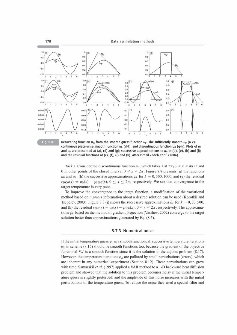
Task 1. Consider the sufficiently smooth function u0 = sin(x), 0 ≤ x ≤ 2π . The functionsu0 and uθ are shown in Fig. 8.8a. Figures 8.8b and c illustrate the iterations ϕk using theiterative scheme similar to Eq. (8.15) for k = 0, 4, 6 and the residual r6(x) = u0(x)−ϕ6(x),0 ≤ x ≤ 2π respectively. We see that iterations converge rather rapid for the sufficientlysmooth target function.
Task 2. Now consider the continuous piece-wise smooth function u0 = 3x/(2π), 0 ≤x ≤ 2π/3 and u0 = 3/2 − 3x/(2π), 2π/3 ≤ x ≤ 2π . Figure 8.8 presents (d) the functionsu0 and uθ , (e) the successive approximations ϕk for k = 0, 4, 1000, and (f) the residualr1000(x) = u0(x) − ϕ1000(x), 0 ≤ x ≤ 2π , respectively. This example shows that a largenumber of iterations is required to reach the target function.
170 Data assimilation methods
Fig. 8.8. Recovering function u0 from the smooth guess function uθ . The sufficiently smooth u0 (a–c);continuous piece-wise smooth function u0 (d–f); and discontinuous function u0 (g–k). Plots of u0and uθ are presented at (a), (d) and (g); successive approximations to u0 at (b), (e), (h) and (j);and the residual functions at (c), (f), (i) and (k). After Ismail-Zadeh et al. (2006).
Task 3. Consider the discontinuous function u0, which takes 1 at 2π/3 ≤ x ≤ 4π/3 and0 in other points of the closed interval 0 ≤ x ≤ 2π . Figure 8.8 presents (g) the functionsu0 and uθ , (h) the successive approximations ϕk for k = 0, 500, 1000, and (e) the residualr1000(x) = u0(x) − ϕ1000(x), 0 ≤ x ≤ 2π , respectively. We see that convergence to thetarget temperature is very poor.
To improve the convergence to the target function, a modification of the variationalmethod based on a priori information about a desired solution can be used (Korotkii andTsepelev, 2003). Figure 8.8 (j) shows the successive approximations ϕ̃k for k = 0, 30, 500,and (k) the residual r̃500(x) = u0(x) − ϕ̃500(x), 0 ≤ x ≤ 2π , respectively. The approxima-tions ϕ̃k based on the method of gradient projection (Vasiliev, 2002) converge to the targetsolution better than approximations generated by Eq. (8.5).
8.7.3 Numerical noise
If the initial temperature guess ϕ0 is a smooth function, all successive temperature iterationsϕk in scheme (8.15) should be smooth functions too, because the gradient of the objectivefunctional ∇J is a smooth function since it is the solution to the adjoint problem (8.17).However, the temperature iterations ϕk are polluted by small perturbations (errors), whichare inherent in any numerical experiment (Section 8.12). These perturbations can growwith time. Samarskii et al. (1997) applied a VAR method to a 1-D backward heat diffusionproblem and showed that the solution to this problem becomes noisy if the initial temper-ature guess is slightly perturbed, and the amplitude of this noise increases with the initialperturbations of the temperature guess. To reduce the noise they used a special filter and
171 8.8 Quasi-reversibility (QRV) method
illustrated the efficiency of the filter. This filter is based on the replacement of iterations(8.15) by the following iterative scheme:
B(ϕk+1 − ϕk) = −βk∇J (ϕk), (8.26)
where By = y − ∇2y. Unfortunately, employment of this filter increases the number ofiterations to obtain the target temperature and it becomes quite expensive computationally,especially when the model is three-dimensional. Another way to reduce the noise is toemploy high-order adjoint (Alekseev and Navon, 2001) or regularisation (Tikhonov, 1963;Lattes and Lions, 1969; Samarskii and Vabischevich, 2004) techniques.
8.8 Quasi-reversibility (QRV) method
The principal idea of the quasi-reversibility (QRV) method is based on the transformationof an ill-posed problem into a well-posed problem (Lattes and Lions, 1969). In the caseof the backward heat equation, this implies an introduction of an additional term into theequation, which involves the product of a small regularisation parameter and higher-ordertemperature derivative. The additional term should be sufficiently small compared to otherterms of the heat equation and allow for simple additional boundary conditions. The dataassimilation in this case is based on a search of the best fit between the forecast modelstate and the observations by minimising the regularisation parameter. The QRV method isproven to be well suited for smooth and non-smooth input data (Lattes and Lions, 1969;Samarskii and Vabishchevich, 2004).
To explain the transformation of the problem, we follow Ismail-Zadeh et al. (2007)and consider the following boundary-value problem for the one-dimensional heat conduc-tion problem
∂T (t, x)
∂t= ∂2T (t, x)
∂x2, 0 ≤ x ≤ π , 0 ≤ t ≤ t∗, (8.27)
T (t, x = 0) = T (t, x = π) = 0, 0 ≤ t ≤ t∗, (8.28)
T (t = 0, x) = 1
4n + 1sin((4n + 1)x), 0 ≤ x ≤ π . (8.29)
The analytical solution to (8.27)–(8.29) can be obtained in the following form
T (t, x) = 1
4n + 1exp(−(4n + 1)2t) sin((4n + 1)x). (8.30)
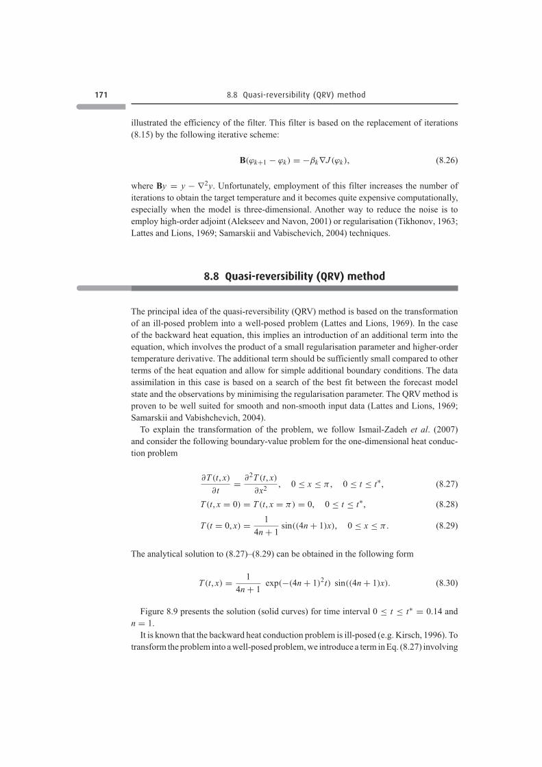
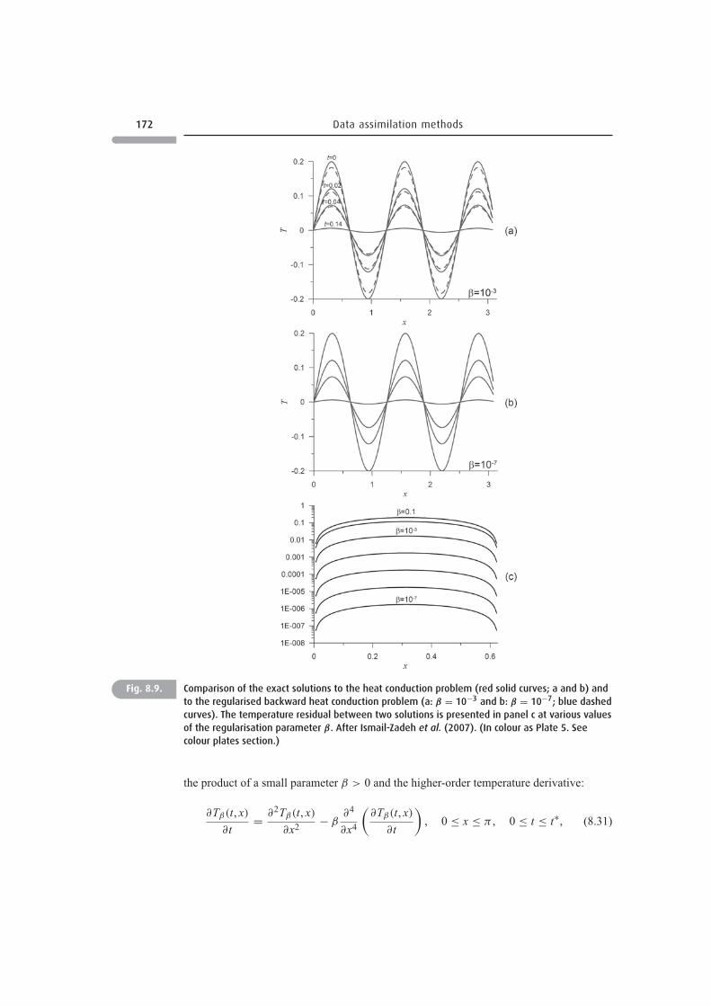
Figure 8.9 presents the solution (solid curves) for time interval 0 ≤ t ≤ t∗ = 0.14 andn = 1.
It is known that the backward heat conduction problem is ill-posed (e.g. Kirsch, 1996). Totransform the problem into a well-posed problem, we introduce a term in Eq. (8.27) involving
172 Data assimilation methods
Fig. 8.9. Comparison of the exact solutions to the heat conduction problem (red solid curves; a and b) andto the regularised backward heat conduction problem (a: β = 10−3 and b: β = 10−7; blue dashedcurves). The temperature residual between two solutions is presented in panel c at various valuesof the regularisation parameter β. After Ismail-Zadeh et al. (2007). (In colour as Plate 5. Seecolour plates section.)
the product of a small parameter β > 0 and the higher-order temperature derivative:
∂Tβ(t, x)
∂t= ∂2Tβ(t, x)
∂x2− β
∂4
∂x4
(∂Tβ(t, x)
∂t
), 0 ≤ x ≤ π , 0 ≤ t ≤ t∗, (8.31)
173 8.8 Quasi-reversibility (QRV) method
Tβ(t, x = 0) = Tβ(t, x = π) = 0, 0 ≤ t ≤ t∗, (8.32)
∂2Tβ(t, x = 0)
∂x2= ∂2Tβ(t, x = π)
∂x2= 0, 0 ≤ t ≤ t∗, (8.33)
Tβ(t = t∗, x) = 1
4n + 1exp(−(4n + 1)2t∗) sin((4n + 1)x), 0 ≤ x ≤ π . (8.34)
Here the initial condition is assumed to be the solution (8.30) to the heat conduction problem(8.27)–(8.29) at t = t∗. The subscript β at Tβ is used to emphasise the dependence of thesolution to problem (8.31)–(8.34) on the regularisation parameter. The analytical solutionto the regularised backward heat conduction problem (8.31)–(8.34) is represented as:
Tβ(t, x) = An exp
( −(4n + 1)2t
1 + β(4n + 1)4
)sin((4n + 1)x),
An = 1
4n + 1exp(−(4n + 1)2t∗) exp−1
( −(4n + 1)2t∗
1 + β(4n + 1)4
), (8.35)
and the solution approaches the initial condition for the problem (8.27)–(8.29) at t = 0 andβ → 0. Figure 8.9a,b illustrates the solution to the regularised problem at two values of β
(dashed curves) and n = 1. The temperature residual (Fig. 8.9c) indicates that the solution(8.35) approaches the solution (8.30) with β → 0.
Samarskii and Vabischevich (2004) estimated the stability of the solution to problem(8.31)–(8.33) with respect to the initial condition expressed in the form Tβ(t = t∗, x) = T ∗
β :
∥∥Tβ(t, x)∥∥ + β
∥∥∂Tβ(t, x)/∂x∥∥ ≤ C
(∥∥∥T ∗β
∥∥∥ + β
∥∥∥∂T ∗β /∂x
∥∥∥) exp[(t∗ − t)β−1/2
],
where C is a constant, and showed that the natural logarithm of errors will increase in directproportion to time and inversely to the root square of the regularisation parameter.
Any regularisation has its advantages and disadvantages. A regularising operator is usedin a mathematical problem to (i) accelerate a convergence; (ii) fulfil the physical laws (e.g.maximum principal, conversation of energy, etc.) in discrete equations; (iii) suppress a noisein input data and in numerical computations; and (iv) take into account a priori informationabout an unknown solution and hence to improve a quality of computations. The majordrawback of regularisation is that the accuracy of the solution to a regularised problem isalways lower than that to a non-regularised problem.
We should mention that the transformation to the regularised backward heat problem isnot only a mathematical approach to solving ill-posed backward heat problems, but hassome physical meaning: it can be explained on the basis of the concept of relaxing heat fluxfor heat conduction (Vernotte, 1958). The classical Fourier heat conduction theory providesthe infinite velocity of heat propagation in a region. The instantaneous heat propagation isunrealistic, because the heat is a result of the vibration of atoms and the vibration prop-agates in a finite speed (Morse and Feshbach, 1953). To accommodate the finite velocityof heat propagation, a modified heat flux model was proposed by Vernotte (1958) andCattaneo (1958).
The modified Fourier constitutive equation (sometimes called the Riemann law of heatconduction) is expressed as �Q = −k∇T − τ ∂ �Q/∂t, where �Q is the heat flux, and k is the
174 Data assimilation methods
coefficient of thermal conductivity. The thermal relaxation time τ = k/(ρcpv
2)
is usuallyrecognised to be a small parameter (Yu et al., 2004), where ρ is the density, cp is the specificheat, and v is the heat propagation velocity. The situation for τ → 0 leads to instantaneousdiffusion at infinite propagation speed, which coincides with the classical thermal diffusiontheory. The heat conduction equation ∂T/∂t = ∇2T +τ ∂2T/∂t2 based on non-Fourier heatflux can be considered as a regularised heat equation. If the Fourier law is modified further
by an addition of the second derivative of heat flux, e.g. �Q = −k∇T +β∂2 �Q∂t2
, where small βis the relaxation parameter of heat flux (Bubnov, 1976, 1981), the heat conduction equationcan be transformed into a higher-order regularised heat equation similar to Eq. (8.31).
8.8.1 The QRV method for restoration of thermo-convective flow
For convenience, we present a set of equations (8.10)–(8.12) with the relevant boundaryand initial conditions as two mathematical problems. Namely, we consider the boundary-value problem for the flow velocity (it includes the Stokes equation, the incompressibilityequation subject to appropriate boundary conditions)
∇P = div (η(T )E) + RaTe, x ∈ �, (8.36)
divu = 0, x ∈ �, (8.37)
u · n = 0, ∂uτ /∂n = 0, x ∈ ∂�, (8.38)
where uτ is the projection of the velocity vector onto the tangent plane at the same point onthe model boundary, and the initial-boundary-value problem for temperature (it includesthe heat equation subject to appropriate boundary and initial conditions)
∂T/∂t + u · ∇T = ∇2T + f , t ∈ [0, ϑ], x ∈ �, (8.39)
σ1T + σ2∂T/∂n = T∗, t ∈ [0, ϑ], x ∈ ∂�, (8.40)
T (0, x) = T0(x), x ∈ �, (8.41)
where T∗ is the given temperature.The direct problem of thermo-convective flow can be formulated as follows: find the
velocity u = u(t, x), the pressure P = P(t, x), and the temperature T = T (t, x) satisfyingboundary value problem (8.36)–(8.38) and initial-boundary-value problem (8.39)–(8.41).We can formulate the inverse problem in this case as follows: find the velocity, pressure,and temperature satisfying boundary-value problem (8.36)–(8.38) and the final-boundaryvalue problem that includes Eqs. (8.39) and (8.40) and the final condition:
T (ϑ , x) = Tϑ(x), x ∈ �, (8.42)
where Tϑ is the temperature at time t = ϑ .To solve the inverse problem by the QRV method, Ismail-Zadeh et al. (2007) considered
the following regularised backward heat problem to define temperature in the past from the
175 8.8 Quasi-reversibility (QRV) method
known temperature Tϑ(x) at present time t = ϑ :
∂Tβ/∂t − uβ · ∇Tβ = ∇2Tβ + f − β�(∂Tβ/∂t), t ∈ [0, ϑ], x ∈ �, (8.43)
σ1Tβ + σ2∂Tβ/∂n = T∗, t ∈ (0, ϑ), x ∈ ∂�, (8.44)
σ1∂2Tβ/∂n2 + σ2∂
3Tβ/∂n3 = 0, t ∈ (0, ϑ), x ∈ ∂�, (8.45)
Tβ(ϑ , x) = Tϑ(x), x ∈ �, (8.46)
where �(T ) = ∂4T/∂x41 + ∂4T/∂x4
2 + ∂4T/∂x43, and the boundary value problem to
determine the fluid flow:
∇Pβ = −div[η(Tβ)E(uβ)
] + RaTβe, x ∈ �, (8.47)
divuβ = 0, x ∈ �, (8.48)
uβ · n = 0 (and/or ∂(uβ)τ /∂n = 0), x ∈ ∂�, (8.49)
where the sign of the velocity field is changed (uβ by −uβ) in Eqs. (8.43) and (8.47) tosimplify the application of the total variation diminishing (TVD) method (see Section 7.9)for solving (8.43)–(8.46). Hereinafter we refer to temperature Tϑ as the input temperature forthe problem (8.43)–(8.49). The core of the transformation of the heat equation is the additionof a high-order differential expression �(∂Tβ/∂t) multiplied by a small parameter β > 0.Note that Eq. (8.45) is added to the boundary conditions to properly define the regularisedbackward heat problem. The solution to the regularised backward heat problem is stable forβ > 0, and the approximate solution to (8.43)–(8.49) converges to the solution of (8.36)–(8.40), and (8.42) in some spaces, where the conditions of well-posedness are met (Samarskiiand Vabischevich, 2004). Thus, the inverse problem of thermo-convective mantle flow isreduced to determination of the velocity uβ = uβ(t, x), the pressure Pβ = Pβ(t, x), and thetemperature Tβ = Tβ(t, x) satisfying (8.43)–(8.49).
8.8.2 Optimisation problem
A maximum of the following functional is sought with respect to the regularisationparameter β:
δ − ∥∥T (t = ϑ , ·; Tβk (t = 0, ·)) − ϕ(·)∥∥ → maxk
, (8.50)
βk = β0qk−1, k = 1, 2, . . . , , (8.51)
where sign ‖ · ‖ denotes the norm in the space L2(�). Since in what follows the dependenceof solutions on initial temperature data is important, we introduce these data explicitly intothe mathematical representation of temperature. Here Tk = Tβk (t = 0, ·) is the solutionto the regularised backward heat problem (8.43)–(8.45) at t = 0; T (t = ϑ , ·; Tk) is thesolution to the heat problem (8.39)–(8.41) at the initial condition T (t = 0, ·) = Tk at timet = ϑ ; ϕ is the known temperature at t = ϑ (the input data on the present temperature);
176 Data assimilation methods
small parameters β0 > 0 and 0 < q < 1 are defined below; and δ > 0 is a given accuracy.When q tends to unity, the computational cost becomes large; and when q tends to zero, theoptimal solution can be missed.
The prescribed accuracy δ is composed from the accuracy of the initial data and theaccuracy of computations. When the input noise decreases and the accuracy of computa-tions increases, the regularisation parameter is expected to decrease. However, estimatesof the initial data errors are usually inaccurate. Estimates of the computation accuracyare not always known, and when they are available, the estimates are coarse. In practi-cal computations, it is more convenient to minimise the following functional with respectto (8.51)
∥∥Tβk+1(t = 0, ·) − Tβk (t = 0, ·)∥∥ → mink
, (8.52)
where misfit between temperatures obtained at two adjacent iterations must be compared.To implement the minimisation of temperature residual (8.50), the inverse problem (8.43)–(8.49) must be solved on the entire time interval as well as the direct problem (8.36)–(8.41) on the same time interval. This at least doubles the amount of computations. Theminimisation of functional (8.52) has a lower computational cost, but it does not rely on apriori information.
8.8.3 Numerical algorithm for QRV data assimilation
In this section we describe the numerical algorithm for solving the inverse problem ofthermo-convective mantle flow using the QRV method. We consider a uniform temporalpartition tn = ϑ − δt n (as defined in Section 8.5) and prescribe some values to parametersβ0, q and (e.g. β0 = 10−3, q = 0.1 and = 10). According to (8.51) a sequence ofthe values of the regularisation parameter {βk} is defined. For each value β = βk modeltemperature and velocity are determined in the following way.
Step 1. Given the temperature Tβ = Tβ(t, ·) at t = tn, the velocity uβ = uβ(tn, ·) is foundby solving problem (8.47)–(8.49). This velocity is assumed to be constant on thetime interval [tn+1, tn].
Step 2. Given the velocity uβ = uβ(tn, ·), the new temperature Tβ = Tβ(t, ·) at t = tn+1
is found on the time interval [tn+1, tn] subject to the final condition Tβ = Tβ(tn, ·)by solving the regularised problem (8.43)–(8.46) backward in time.
Step 3. Upon the completion of steps 1 and 2 for all n = 0, 1, . . . , m, the temperatureTβ = Tβ(tn, ·) and the velocity uβ = uβ(tn, ·) are obtained at each t = tn. Basedon the computed solution we can find the temperature and flow velocity at eachpoint of time interval [0, ϑ] using interpolation.
Step 4a. The direct problem (8.39)–(8.41) is solved assuming that the initial temperatureis given as Tβ = Tβ(t = 0, ·), and the temperature residual (8.50) is found. If theresidual does not exceed the predefined accuracy, the calculations are terminated,and the results obtained at step 3 are considered as the final ones. Otherwise,
177 8.9 Application of the QRV method: mantle plume evolution
parameters β0, q and entering Eq. (8.51) are modified, and the calculations arecontinued from step 1 for new set {βk}.
Step 4b. The functional (8.52) is calculated. If the residual between the solutions obtainedfor two adjacent regularisation parameters satisfies a predefined criterion (thecriterion should be defined by a user, because no a priori data are used at this step),the calculation is terminated, and the results obtained at step 3 are considered asthe final ones. Otherwise, parameters β0, q and entering Eq. (8.51) are modified,and the calculations are continued from step 1 for new set {βk}.
In a particular implementation, either step 4a or step 4b is used to terminate the computa-tion. This algorithm allows (i) organising a certain number of independent computationalmodules for various values of the regularised parameter βk that find the solution to theregularised problem using steps 1–3 and (ii) determining a posteriori an acceptable resultaccording to step 4a or step 4b.
8.9 Application of the QRV method: mantle plume evolution
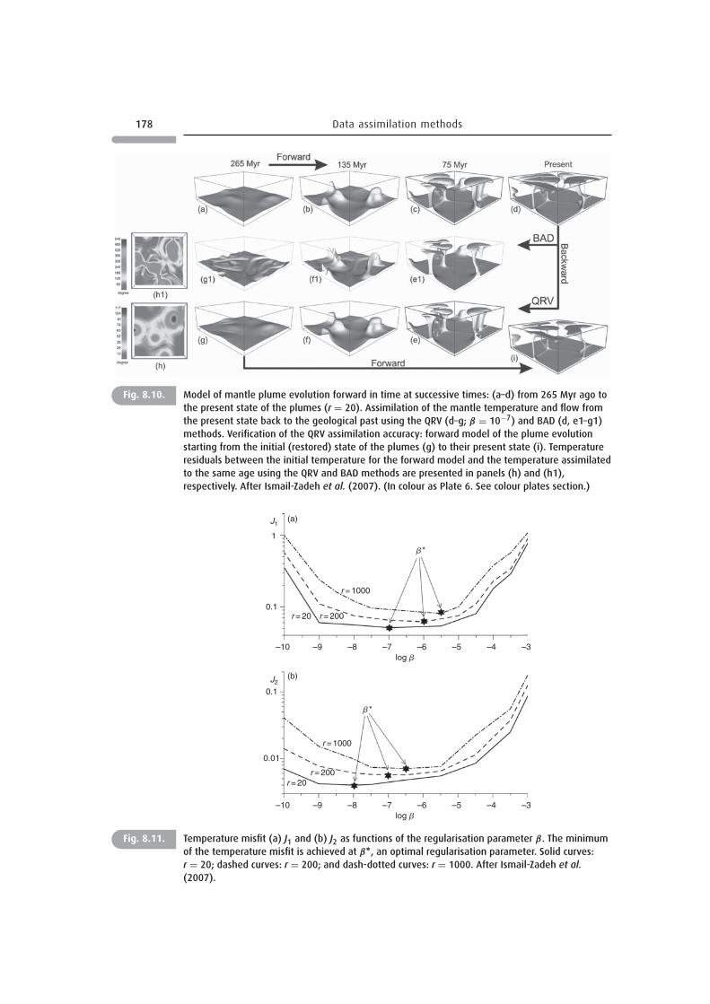
To compare the numerical results obtained by the QRV method with that obtained by theVAR and BAD methods described in this chapter, we develop the same forward model formantle plume evolution as presented in Section 8.6. Figure 8.10 (panels a–d) illustrates theevolution of mantle plumes in the forward model. The state of the plumes at the ‘present’time (Fig. 8.10d) obtained by solving the direct problem was used as the input temperaturefor the inverse problem (an assimilation of the ‘present’ temperature to the past). Notethat this initial state (input temperature) is given with an error introduced by the numericalalgorithm used to solve the direct problem. Figure 8.10 illustrates the states of the plumesrestored by the QRV method (panels e–g) and the residual δT (see Eq. (8.26) and panel h)between the initial temperature for the forward model (Fig. 8.10a) and the temperature T̃ (x)
assimilated to the same age (Fig. 8.10g). To check the stability of the algorithm, a forwardmodel of the restored plumes is computed using the solution to the inverse problem at thetime of 265 Myr ago (Fig. 8.10g) as the initial state for the forward model. The result ofthis run is shown in Fig. 8.10i.
To compare the accuracy of the data assimilation methods, a restoration model from the‘present’time (Fig. 8.10d) to the time of 265 Myr ago was developed using the BAD method.Figure 8.10 shows the BAD model results (panels e1–g1) together with the temperatureresidual (panel h1) between the initial temperature (panel a) and the temperature assimilatedto the same age (panel g1). The VAR method was not used to assimilate data within the timeinterval of more than 100 Myr (for Ra ≈ 106), because proper filtering of the increasingnoise is required to smooth the input data and solution (Section 8.7).
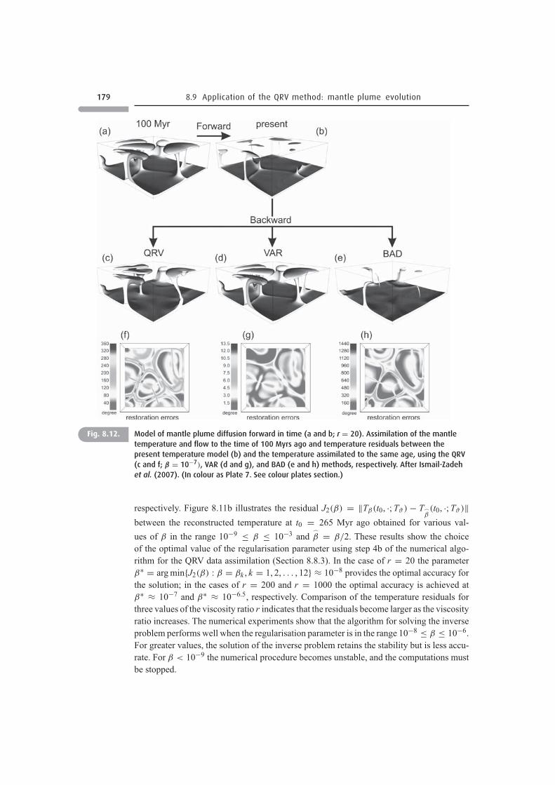
Figure 8.11a presents the residual J1(β) = ‖T0(·) − Tβ(t = t0, ·; Tϑ)‖ between the initialtemperature T0 at t0 = 265 Myr ago and the restored temperature (to the same time) obtainedby solving the inverse problem with the input temperature Tϑ . The optimal accuracy isattained at β∗ = arg min{J1(β) : β = βk , k = 1, 2, . . . , 10} ≈ 10−7 in the case of r = 20,and at β∗ ≈ 10−6 and β∗ ≈ 10−5.5 in the cases of the viscosity ratio r = 200 and r = 1000,
178 Data assimilation methods
Fig. 8.10. Model of mantle plume evolution forward in time at successive times: (a–d) from 265 Myr ago tothe present state of the plumes (r = 20). Assimilation of the mantle temperature and flow fromthe present state back to the geological past using the QRV (d–g; β = 10−7) and BAD (d, e1–g1)methods. Verification of the QRV assimilation accuracy: forward model of the plume evolutionstarting from the initial (restored) state of the plumes (g) to their present state (i). Temperatureresiduals between the initial temperature for the forward model and the temperature assimilatedto the same age using the QRV and BAD methods are presented in panels (h) and (h1),respectively. After Ismail-Zadeh et al. (2007). (In colour as Plate 6. See colour plates section.)
(a)
(b)
J1
J2
1
–10 –9 –8
r = 1000
r = 1000
r = 200
r = 200
r = 20
r = 20
–7log b
b*
b*
–6 –5 –4 –3
–10 –9 –8 –7log b
–6 –5 –4 –3
0.1
0.1
0.01
Fig. 8.11. Temperature misfit (a) J1 and (b) J2 as functions of the regularisation parameter β. The minimumof the temperature misfit is achieved at β∗, an optimal regularisation parameter. Solid curves:r = 20; dashed curves: r = 200; and dash-dotted curves: r = 1000. After Ismail-Zadeh et al.(2007).
179 8.9 Application of the QRV method: mantle plume evolution
Fig. 8.12. Model of mantle plume diffusion forward in time (a and b; r = 20). Assimilation of the mantletemperature and flow to the time of 100 Myrs ago and temperature residuals between thepresent temperature model (b) and the temperature assimilated to the same age, using the QRV(c and f; β = 10−7), VAR (d and g), and BAD (e and h) methods, respectively. After Ismail-Zadehet al. (2007). (In colour as Plate 7. See colour plates section.)
respectively. Figure 8.11b illustrates the residual J2(β) = ‖Tβ(t0, ·; Tϑ) − T�β(t0, ·; Tϑ)‖
between the reconstructed temperature at t0 = 265 Myr ago obtained for various val-
ues of β in the range 10−9 ≤ β ≤ 10−3 and�
β = β/2. These results show the choiceof the optimal value of the regularisation parameter using step 4b of the numerical algo-rithm for the QRV data assimilation (Section 8.8.3). In the case of r = 20 the parameterβ∗ = arg min{J2(β) : β = βk , k = 1, 2, . . . , 12} ≈ 10−8 provides the optimal accuracy forthe solution; in the cases of r = 200 and r = 1000 the optimal accuracy is achieved atβ∗ ≈ 10−7 and β∗ ≈ 10−6.5, respectively. Comparison of the temperature residuals forthree values of the viscosity ratio r indicates that the residuals become larger as the viscosityratio increases. The numerical experiments show that the algorithm for solving the inverseproblem performs well when the regularisation parameter is in the range 10−8 ≤ β ≤ 10−6.For greater values, the solution of the inverse problem retains the stability but is less accu-rate. For β < 10−9 the numerical procedure becomes unstable, and the computations mustbe stopped.
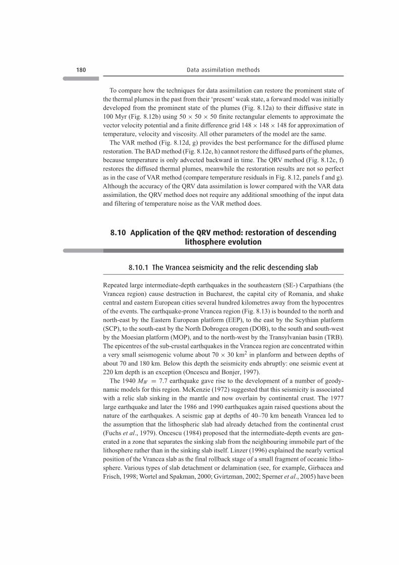
180 Data assimilation methods
To compare how the techniques for data assimilation can restore the prominent state ofthe thermal plumes in the past from their ‘present’weak state, a forward model was initiallydeveloped from the prominent state of the plumes (Fig. 8.12a) to their diffusive state in100 Myr (Fig. 8.12b) using 50 × 50 × 50 finite rectangular elements to approximate thevector velocity potential and a finite difference grid 148 × 148 × 148 for approximation oftemperature, velocity and viscosity. All other parameters of the model are the same.
The VAR method (Fig. 8.12d, g) provides the best performance for the diffused plumerestoration. The BAD method (Fig. 8.12e, h) cannot restore the diffused parts of the plumes,because temperature is only advected backward in time. The QRV method (Fig. 8.12c, f)restores the diffused thermal plumes, meanwhile the restoration results are not so perfectas in the case of VAR method (compare temperature residuals in Fig. 8.12, panels f and g).Although the accuracy of the QRV data assimilation is lower compared with the VAR dataassimilation, the QRV method does not require any additional smoothing of the input dataand filtering of temperature noise as the VAR method does.
8.10 Application of the QRV method: restoration of descendinglithosphere evolution
8.10.1 The Vrancea seismicity and the relic descending slab
Repeated large intermediate-depth earthquakes in the southeastern (SE-) Carpathians (theVrancea region) cause destruction in Bucharest, the capital city of Romania, and shakecentral and eastern European cities several hundred kilometres away from the hypocentresof the events. The earthquake-prone Vrancea region (Fig. 8.13) is bounded to the north andnorth-east by the Eastern European platform (EEP), to the east by the Scythian platform(SCP), to the south-east by the North Dobrogea orogen (DOB), to the south and south-westby the Moesian platform (MOP), and to the north-west by the Transylvanian basin (TRB).The epicentres of the sub-crustal earthquakes in the Vrancea region are concentrated withina very small seismogenic volume about 70 × 30 km2 in planform and between depths ofabout 70 and 180 km. Below this depth the seismicity ends abruptly: one seismic event at220 km depth is an exception (Oncescu and Bonjer, 1997).
The 1940 MW = 7.7 earthquake gave rise to the development of a number of geody-namic models for this region. McKenzie (1972) suggested that this seismicity is associatedwith a relic slab sinking in the mantle and now overlain by continental crust. The 1977large earthquake and later the 1986 and 1990 earthquakes again raised questions about thenature of the earthquakes. A seismic gap at depths of 40–70 km beneath Vrancea led tothe assumption that the lithospheric slab had already detached from the continental crust(Fuchs et al., 1979). Oncescu (1984) proposed that the intermediate-depth events are gen-erated in a zone that separates the sinking slab from the neighbouring immobile part of thelithosphere rather than in the sinking slab itself. Linzer (1996) explained the nearly verticalposition of the Vrancea slab as the final rollback stage of a small fragment of oceanic litho-sphere. Various types of slab detachment or delamination (see, for example, Girbacea andFrisch, 1998; Wortel and Spakman, 2000; Gvirtzman, 2002; Sperner et al., 2005) have been
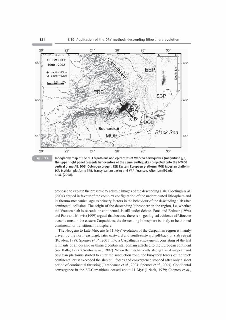
181 8.10 Application of the QRV method: descending lithosphere evolution
Fig. 8.13. Topography map of the SE-Carpathians and epicentres of Vrancea earthquakes (magnitude ≥3).The upper right panel presents hypocentres of the same earthquakes projected onto the NW–SEvertical plane AB. DOB, Dobrogea orogen; EEP, Eastern European platform; MOP, Moesian platform;SCP, Scythian platform; TRB, Transylvanian basin; and VRA, Vrancea. After Ismail-Zadehet al. (2008).
proposed to explain the present-day seismic images of the descending slab. Cloetingh et al.(2004) argued in favour of the complex configuration of the underthrusted lithosphere andits thermo-mechanical age as primary factors in the behaviour of the descending slab aftercontinental collision. The origin of the descending lithosphere in the region, i.e. whetherthe Vrancea slab is oceanic or continental, is still under debate. Pana and Erdmer (1996)and Pana and Morris (1999) argued that because there is no geological evidence of Mioceneoceanic crust in the eastern Carpathians, the descending lithosphere is likely to be thinnedcontinental or transitional lithosphere.
The Neogene to Late Miocene (c 11 Myr) evolution of the Carpathian region is mainlydriven by the north-eastward, later eastward and south-eastward roll-back or slab retreat(Royden, 1988; Sperner et al., 2001) into a Carpathians embayment, consisting of the lastremnants of an oceanic or thinned continental domain attached to the European continent(see Balla, 1987; Csontos et al., 1992). When the mechanically strong East-European andScythian platforms started to enter the subduction zone, the buoyancy forces of the thickcontinental crust exceeded the slab pull forces and convergence stopped after only a shortperiod of continental thrusting (Tarapoanca et al., 2004; Sperner et al., 2005). Continentalconvergence in the SE-Carpathians ceased about 11 Myr (Jiricek, 1979; Csontos et al.,
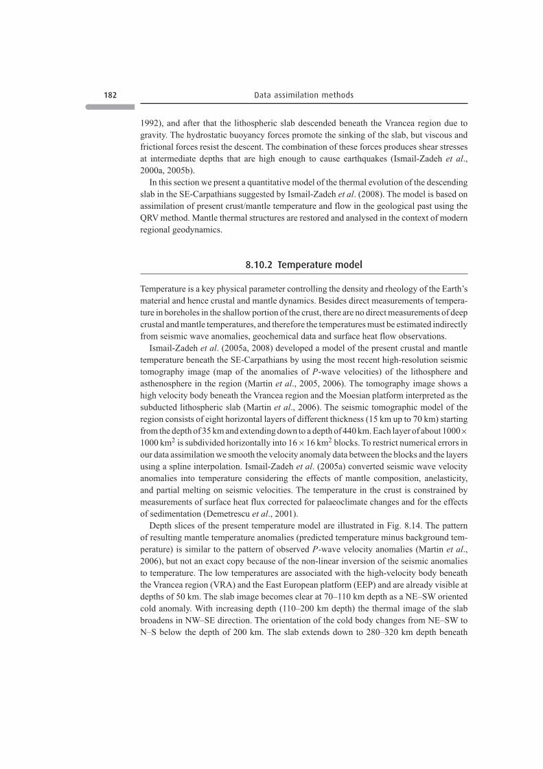
182 Data assimilation methods
1992), and after that the lithospheric slab descended beneath the Vrancea region due togravity. The hydrostatic buoyancy forces promote the sinking of the slab, but viscous andfrictional forces resist the descent. The combination of these forces produces shear stressesat intermediate depths that are high enough to cause earthquakes (Ismail-Zadeh et al.,2000a, 2005b).
In this section we present a quantitative model of the thermal evolution of the descendingslab in the SE-Carpathians suggested by Ismail-Zadeh et al. (2008). The model is based onassimilation of present crust/mantle temperature and flow in the geological past using theQRV method. Mantle thermal structures are restored and analysed in the context of modernregional geodynamics.
8.10.2 Temperature model
Temperature is a key physical parameter controlling the density and rheology of the Earth’smaterial and hence crustal and mantle dynamics. Besides direct measurements of tempera-ture in boreholes in the shallow portion of the crust, there are no direct measurements of deepcrustal and mantle temperatures, and therefore the temperatures must be estimated indirectlyfrom seismic wave anomalies, geochemical data and surface heat flow observations.
Ismail-Zadeh et al. (2005a, 2008) developed a model of the present crustal and mantletemperature beneath the SE-Carpathians by using the most recent high-resolution seismictomography image (map of the anomalies of P-wave velocities) of the lithosphere andasthenosphere in the region (Martin et al., 2005, 2006). The tomography image shows ahigh velocity body beneath the Vrancea region and the Moesian platform interpreted as thesubducted lithospheric slab (Martin et al., 2006). The seismic tomographic model of theregion consists of eight horizontal layers of different thickness (15 km up to 70 km) startingfrom the depth of 35 km and extending down to a depth of 440 km. Each layer of about 1000×1000 km2 is subdivided horizontally into 16×16 km2 blocks. To restrict numerical errors inour data assimilation we smooth the velocity anomaly data between the blocks and the layersusing a spline interpolation. Ismail-Zadeh et al. (2005a) converted seismic wave velocityanomalies into temperature considering the effects of mantle composition, anelasticity,and partial melting on seismic velocities. The temperature in the crust is constrained bymeasurements of surface heat flux corrected for palaeoclimate changes and for the effectsof sedimentation (Demetrescu et al., 2001).
Depth slices of the present temperature model are illustrated in Fig. 8.14. The patternof resulting mantle temperature anomalies (predicted temperature minus background tem-perature) is similar to the pattern of observed P-wave velocity anomalies (Martin et al.,2006), but not an exact copy because of the non-linear inversion of the seismic anomaliesto temperature. The low temperatures are associated with the high-velocity body beneaththe Vrancea region (VRA) and the East European platform (EEP) and are already visible atdepths of 50 km. The slab image becomes clear at 70–110 km depth as a NE–SW orientedcold anomaly. With increasing depth (110–200 km depth) the thermal image of the slabbroadens in NW–SE direction. The orientation of the cold body changes from NE–SW toN–S below the depth of 200 km. The slab extends down to 280–320 km depth beneath
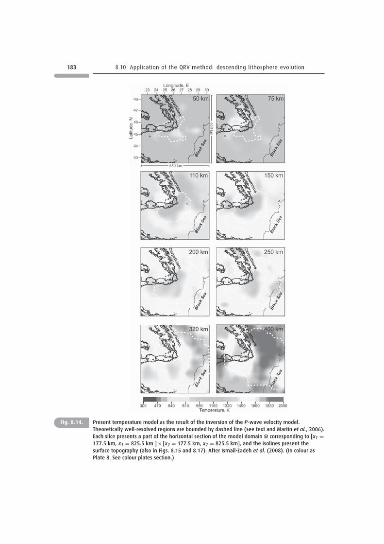
183 8.10 Application of the QRV method: descending lithosphere evolution
Fig. 8.14. Present temperature model as the result of the inversion of the P-wave velocity model.Theoretically well-resolved regions are bounded by dashed line (see text and Martin et al., 2006).Each slice presents a part of the horizontal section of the model domain � corresponding to [x1 =177.5 km, x1 = 825.5 km ]× [x2 = 177.5 km, x2 = 825.5 km], and the isolines present thesurface topography (also in Figs. 8.15 and 8.17). After Ismail-Zadeh et al. (2008). (In colour asPlate 8. See colour plates section.)
184 Data assimilation methods
the Vrancea region itself. A cold anomaly beneath the Transylvanian Basin is estimated atdepths of 370–440 km. According to Wortel and Spakman (2000) and Martin et al. (2006)this cold material can be interpreted as a remnant of subducted lithosphere detached dur-ing the Miocene along the Carpathian Arc and residing within the upper mantle transitionzone. High temperatures are predicted beneath the Transylvanian Basin (TRB) at about 70–110 km depth. Two other high temperature regions are found at 110–150 km depth below theMoesian platform (MOP) and deeper than 200 km under the EEP and the Dobrogea orogen(DOB), which might be correlated with the regional lithosphere/asthenosphere boundary.
8.10.3 QRV data assimilation
To minimise boundary effects, the studied region (650 × 650 km2 and 440 km deep, seeFig. 8.14) has been bordered horizontally by a 200 km area and extended vertically to thedepth of 670 km. Therefore, a rectangular domain � = [0, l1 = 1050 km] × [0, l2 =1050 km] × [0, h = 670 km] is considered for assimilation of present temperature andmantle flow beneath the SE-Carpathians.
Our ability to reverse mantle flow is limited by our knowledge of past movements inthe region, which are well constrained in only some cases. In reality, the Earth’s crust andlithospheric mantle are driven by mantle convection and the gravitational pull of densedescending slabs. However, when a numerical model is constructed for a particular region,external lateral forces can influence the regional crustal and uppermost mantle movements.Yet in order to make useful predictions that can be tested geologically, a time-dependentnumerical model should include the history of surface motions. Since this is not currentlyachievable in a dynamical way, it is necessary to prescribe surface motions by using velocityboundary conditions.
The simulations are performed backward in time for a period of 22 Myr. Perfect slipconditions are assumed at the vertical and lower boundaries of the model domain. For thefirst 11 Myr (starting from the present time), when the rates of continental convergence wereinsignificant (Jiricek, 1979; Csontos et al., 1992), no velocity is imposed at the surface, andthe conditions at the upper boundary are free slip. The north-westward velocity is imposedin the portion of the upper model boundary (Fig. 8.15a) for the time interval from 11 Myr to16 Myr and the westward velocity in the same portion of the boundary (Fig. 8.15b) for theinterval from 16 Myr to 22 Myr. The velocities are consistent with the direction and rates ofthe regional convergence in the Early and Middle Miocene (Morley, 1996; Fügenschuh andSchmid, 2005; Sperner et al., 2005). The effect of the surface loading due to the CarpathianMountains is not considered, because this loading would have insignificant influence onthe dynamics of the region (as was shown in two-dimensional models of the Vrancea slabevolution; Ismail-Zadeh et al., 2005b).
The heat flux through the vertical boundaries of the model domain � is set to zero. Theupper and lower boundaries are assumed to be isothermal surfaces. The present temperatureabove 440 km depth is derived from the seismic velocity anomalies and heat flow data. Theadiabatic geotherm for potential temperature 1750 K (Katsura et al., 2004) was used todefine the present temperature below 440 km (where seismic tomography data are not
185 8.10 Application of the QRV method: descending lithosphere evolution
Fig. 8.15. Surface velocity imposed on the part of the upper boundary of the model domain (see the captionof Fig. 8.14) in data assimilation modelling for the time interval from 11 Myr to 16 Myr ago (a)and for that from 16 Myr to 22 Myr ago (b). After Ismail-Zadeh et al. (2008).
available). Equations (8.36)–(8.49) with the specified boundary and initial conditions aresolved numerically.
To estimate the accuracy of the results of data assimilation, the temperature and mantleflow restored to the time of 22 Myr ago were employed as the initial condition for a modelof the slab evolution forward in time; the model was run to the present; and the temperatureresidual (the difference between the present temperature and that predicted by the forwardmodel with the restored temperature as an initial temperature distribution) was analysedsubsequently. The maximum temperature residual does not exceed 50 K.
A sensitivity analysis was performed to understand how stable is the numerical solutionto small perturbations of input (present) temperatures. The model of the present temperature(Section 8.10.2) has been perturbed randomly by 0.5% to 2% and then assimilated to thepast to find the initial temperature. A misfit between the initial temperatures related to theperturbed and unperturbed present temperature is rather small (2% to 4%), which provesthat the solution is stable. The numerical models, with a spatial resolution of 7 km ×7 km × 5 km, were run on parallel computers. The accuracy of the numerical solutionshas been verified by several tests, including grid and total mass changes (Ismail-Zadehet al., 2001a).
8.10.4 What the past tells us
We discuss here the results of assimilation of the present temperature model beneath the SE-Carpathians into Miocene times. Although there is some evidence that the lithospheric slabwas already partly subducted some 75 Myr ago (Sandulescu, 1988), the assimilation intervalwas restricted to the Miocene, because the pre-Miocene evolution of the descending slab, aswell as the regional horizontal movements, are poorly known. Incorporation of insufficiently
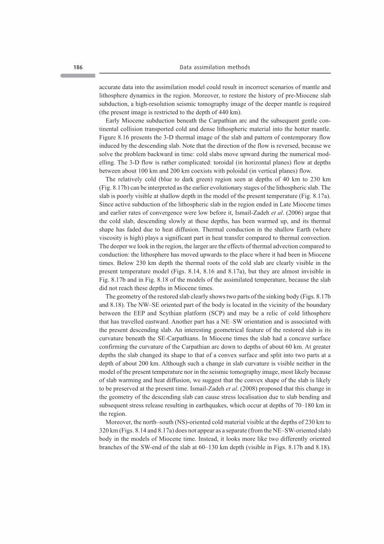
186 Data assimilation methods
accurate data into the assimilation model could result in incorrect scenarios of mantle andlithosphere dynamics in the region. Moreover, to restore the history of pre-Miocene slabsubduction, a high-resolution seismic tomography image of the deeper mantle is required(the present image is restricted to the depth of 440 km).
Early Miocene subduction beneath the Carpathian arc and the subsequent gentle con-tinental collision transported cold and dense lithospheric material into the hotter mantle.Figure 8.16 presents the 3-D thermal image of the slab and pattern of contemporary flowinduced by the descending slab. Note that the direction of the flow is reversed, because wesolve the problem backward in time: cold slabs move upward during the numerical mod-elling. The 3-D flow is rather complicated: toroidal (in horizontal planes) flow at depthsbetween about 100 km and 200 km coexists with poloidal (in vertical planes) flow.
The relatively cold (blue to dark green) region seen at depths of 40 km to 230 km(Fig. 8.17b) can be interpreted as the earlier evolutionary stages of the lithospheric slab. Theslab is poorly visible at shallow depth in the model of the present temperature (Fig. 8.17a).Since active subduction of the lithospheric slab in the region ended in Late Miocene timesand earlier rates of convergence were low before it, Ismail-Zadeh et al. (2006) argue thatthe cold slab, descending slowly at these depths, has been warmed up, and its thermalshape has faded due to heat diffusion. Thermal conduction in the shallow Earth (whereviscosity is high) plays a significant part in heat transfer compared to thermal convection.The deeper we look in the region, the larger are the effects of thermal advection compared toconduction: the lithosphere has moved upwards to the place where it had been in Miocenetimes. Below 230 km depth the thermal roots of the cold slab are clearly visible in thepresent temperature model (Figs. 8.14, 8.16 and 8.17a), but they are almost invisible inFig. 8.17b and in Fig. 8.18 of the models of the assimilated temperature, because the slabdid not reach these depths in Miocene times.
The geometry of the restored slab clearly shows two parts of the sinking body (Figs. 8.17band 8.18). The NW–SE oriented part of the body is located in the vicinity of the boundarybetween the EEP and Scythian platform (SCP) and may be a relic of cold lithospherethat has travelled eastward. Another part has a NE–SW orientation and is associated withthe present descending slab. An interesting geometrical feature of the restored slab is itscurvature beneath the SE-Carpathians. In Miocene times the slab had a concave surfaceconfirming the curvature of the Carpathian arc down to depths of about 60 km. At greaterdepths the slab changed its shape to that of a convex surface and split into two parts at adepth of about 200 km. Although such a change in slab curvature is visible neither in themodel of the present temperature nor in the seismic tomography image, most likely becauseof slab warming and heat diffusion, we suggest that the convex shape of the slab is likelyto be preserved at the present time. Ismail-Zadeh et al. (2008) proposed that this change inthe geometry of the descending slab can cause stress localisation due to slab bending andsubsequent stress release resulting in earthquakes, which occur at depths of 70–180 km inthe region.
Moreover, the north–south (NS)-oriented cold material visible at the depths of 230 km to320 km (Figs. 8.14 and 8.17a) does not appear as a separate (from the NE–SW-oriented slab)body in the models of Miocene time. Instead, it looks more like two differently orientedbranches of the SW-end of the slab at 60–130 km depth (visible in Figs. 8.17b and 8.18).
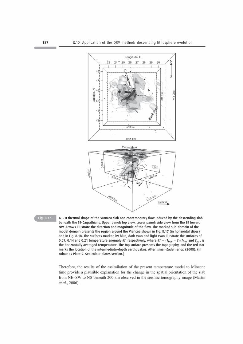
187 8.10 Application of the QRV method: descending lithosphere evolution
Fig. 8.16. A 3-D thermal shape of the Vrancea slab and contemporary flow induced by the descending slabbeneath the SE-Carpathians. Upper panel: top view. Lower panel: side view from the SE towardNW. Arrows illustrate the direction and magnitude of the flow. The marked sub-domain of themodel domain presents the region around the Vrancea shown in Fig. 8.17 (in horizontal slices)and in Fig. 8.18. The surfaces marked by blue, dark cyan and light cyan illustrate the surfaces of0.07, 0.14 and 0.21 temperature anomaly δT, respectively, where δT = (Thav − T)/Thav and Thav isthe horizontally averaged temperature. The top surface presents the topography, and the red starmarks the location of the intermediate-depth earthquakes. After Ismail-Zadeh et al. (2008). (Incolour as Plate 9. See colour plates section.)
Therefore, the results of the assimilation of the present temperature model to Miocenetime provide a plausible explanation for the change in the spatial orientation of the slabfrom NE–SW to NS beneath 200 km observed in the seismic tomography image (Martinet al., 2006).
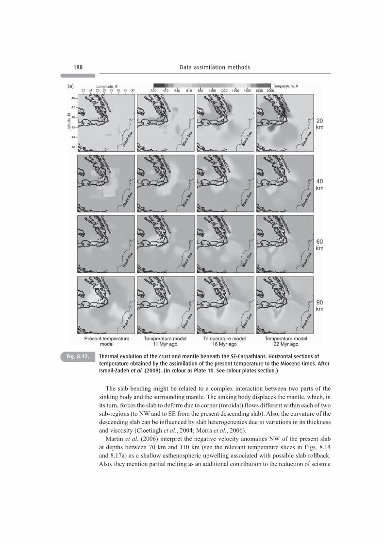
188 Data assimilation methods
(a)
Fig. 8.17. Thermal evolution of the crust and mantle beneath the SE-Carpathians. Horizontal sections oftemperature obtained by the assimilation of the present temperature to the Miocene times. AfterIsmail-Zadeh et al. (2008). (In colour as Plate 10. See colour plates section.)
The slab bending might be related to a complex interaction between two parts of thesinking body and the surrounding mantle. The sinking body displaces the mantle, which, inits turn, forces the slab to deform due to corner (toroidal) flows different within each of twosub-regions (to NW and to SE from the present descending slab). Also, the curvature of thedescending slab can be influenced by slab heterogeneities due to variations in its thicknessand viscosity (Cloetingh et al., 2004; Morra et al., 2006).
Martin et al. (2006) interpret the negative velocity anomalies NW of the present slabat depths between 70 km and 110 km (see the relevant temperature slices in Figs. 8.14and 8.17a) as a shallow asthenospheric upwelling associated with possible slab rollback.Also, they mention partial melting as an additional contribution to the reduction of seismic
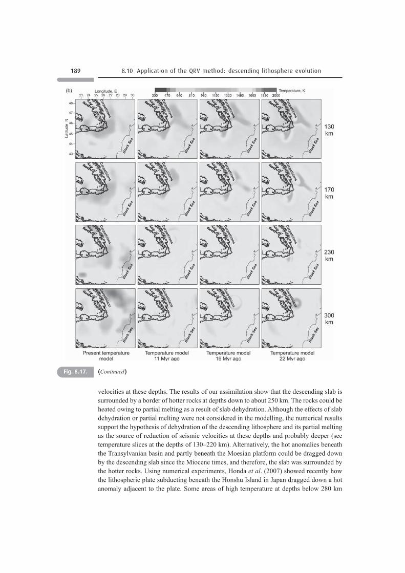
189 8.10 Application of the QRV method: descending lithosphere evolution
(b)
Fig. 8.17. (Continued)
velocities at these depths. The results of our assimilation show that the descending slab issurrounded by a border of hotter rocks at depths down to about 250 km. The rocks could beheated owing to partial melting as a result of slab dehydration. Although the effects of slabdehydration or partial melting were not considered in the modelling, the numerical resultssupport the hypothesis of dehydration of the descending lithosphere and its partial meltingas the source of reduction of seismic velocities at these depths and probably deeper (seetemperature slices at the depths of 130–220 km). Alternatively, the hot anomalies beneaththe Transylvanian basin and partly beneath the Moesian platform could be dragged downby the descending slab since the Miocene times, and therefore, the slab was surrounded bythe hotter rocks. Using numerical experiments, Honda et al. (2007) showed recently howthe lithospheric plate subducting beneath the Honshu Island in Japan dragged down a hotanomaly adjacent to the plate. Some areas of high temperature at depths below 280 km
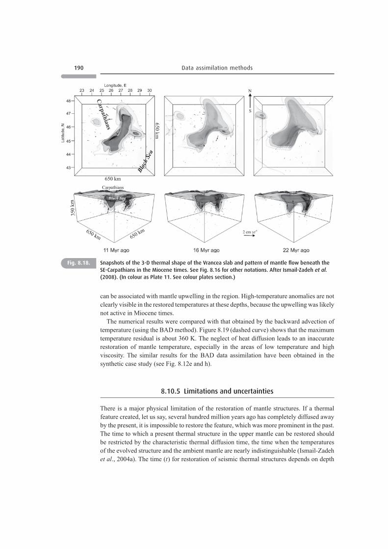
190 Data assimilation methods
Fig. 8.18. Snapshots of the 3-D thermal shape of the Vrancea slab and pattern of mantle flow beneath theSE-Carpathians in the Miocene times. See Fig. 8.16 for other notations. After Ismail-Zadeh et al.(2008). (In colour as Plate 11. See colour plates section.)
can be associated with mantle upwelling in the region. High-temperature anomalies are notclearly visible in the restored temperatures at these depths, because the upwelling was likelynot active in Miocene times.
The numerical results were compared with that obtained by the backward advection oftemperature (using the BAD method). Figure 8.19 (dashed curve) shows that the maximumtemperature residual is about 360 K. The neglect of heat diffusion leads to an inaccuraterestoration of mantle temperature, especially in the areas of low temperature and highviscosity. The similar results for the BAD data assimilation have been obtained in thesynthetic case study (see Fig. 8.12e and h).
8.10.5 Limitations and uncertainties
There is a major physical limitation of the restoration of mantle structures. If a thermalfeature created, let us say, several hundred million years ago has completely diffused awayby the present, it is impossible to restore the feature, which was more prominent in the past.The time to which a present thermal structure in the upper mantle can be restored shouldbe restricted by the characteristic thermal diffusion time, the time when the temperaturesof the evolved structure and the ambient mantle are nearly indistinguishable (Ismail-Zadehet al., 2004a). The time (t) for restoration of seismic thermal structures depends on depth
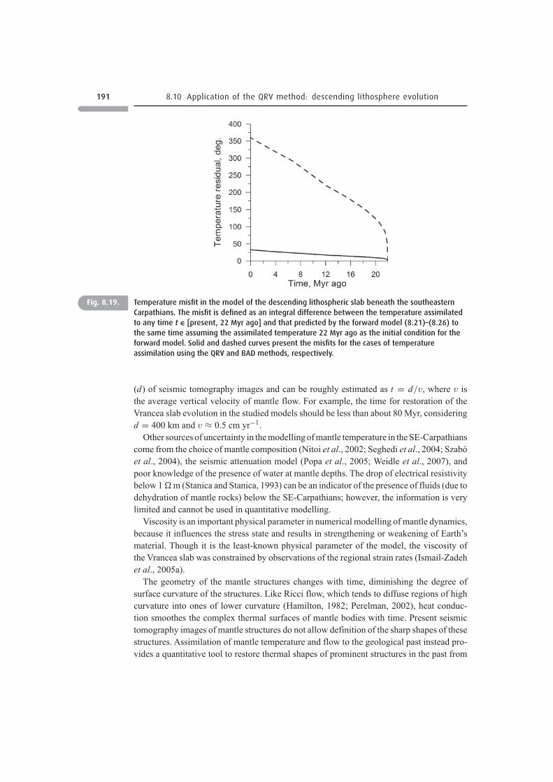
191 8.10 Application of the QRV method: descending lithosphere evolution
Fig. 8.19. Temperature misfit in the model of the descending lithospheric slab beneath the southeasternCarpathians. The misfit is defined as an integral difference between the temperature assimilatedto any time t ∈ [present, 22 Myr ago] and that predicted by the forward model (8.21)–(8.26) tothe same time assuming the assimilated temperature 22 Myr ago as the initial condition for theforward model. Solid and dashed curves present the misfits for the cases of temperatureassimilation using the QRV and BAD methods, respectively.
(d) of seismic tomography images and can be roughly estimated as t = d/v, where v isthe average vertical velocity of mantle flow. For example, the time for restoration of theVrancea slab evolution in the studied models should be less than about 80 Myr, consideringd = 400 km and v ≈ 0.5 cm yr−1.
Other sources of uncertainty in the modelling of mantle temperature in the SE-Carpathianscome from the choice of mantle composition (Nitoi et al., 2002; Seghedi et al., 2004; Szabóet al., 2004), the seismic attenuation model (Popa et al., 2005; Weidle et al., 2007), andpoor knowledge of the presence of water at mantle depths. The drop of electrical resistivitybelow 1 � m (Stanica and Stanica, 1993) can be an indicator of the presence of fluids (due todehydration of mantle rocks) below the SE-Carpathians; however, the information is verylimited and cannot be used in quantitative modelling.
Viscosity is an important physical parameter in numerical modelling of mantle dynamics,because it influences the stress state and results in strengthening or weakening of Earth’smaterial. Though it is the least-known physical parameter of the model, the viscosity ofthe Vrancea slab was constrained by observations of the regional strain rates (Ismail-Zadehet al., 2005a).
The geometry of the mantle structures changes with time, diminishing the degree ofsurface curvature of the structures. Like Ricci flow, which tends to diffuse regions of highcurvature into ones of lower curvature (Hamilton, 1982; Perelman, 2002), heat conduc-tion smoothes the complex thermal surfaces of mantle bodies with time. Present seismictomography images of mantle structures do not allow definition of the sharp shapes of thesestructures. Assimilation of mantle temperature and flow to the geological past instead pro-vides a quantitative tool to restore thermal shapes of prominent structures in the past from
192 Data assimilation methods
their diffusive shapes at present. High-resolution experiments on seismic wave attenuation,improved knowledge of crustal and mantle mineral composition, accurate GPS measure-ments of regional movements, and precise geological palaeoreconstructions of crustalmovements will assist to refine the present models and our knowledge of the regional ther-mal evolutions. The basic knowledge we have gained from the case studies is the dynamicsof the Earth’s interior in the past, which could result in its present dynamics.
8.11 Comparison of data assimilation methods
We compare the VAR, QRV and BAD methods in terms of solution stability, convergence,and accuracy, time interval for data assimilation, analytical and algorithmic works, and com-puter performance (see Tables 8.1–8.3). The VAR data assimilation assumes that the directand adjoint problems are constructed and solved iteratively forward in time. The structure ofthe adjoint problem is identical to the structure of the original problem, which considerablysimplifies the numerical implementation. However, the VAR method imposes some require-ments for the mathematical model (i.e. a derivation of the adjoint problem). Moreover, for anefficient numerical implementation of the VAR method, the error level of the computationsmust be adjusted to the parameters of the algorithm, and this complicates computations.
The QRV method allows employing sophisticated mathematical models (because it doesnot require derivation of an adjoint problem as in the VAR data assimilation) and henceexpands the scope for applications in geodynamics (e.g. thermo-chemical convection, phasetransformations in the mantle). It does not require that the desired accuracy of computationsbe directly related to the parameters of the numerical algorithm. However, the regularisingoperators usually used in the QRV method enhance the order of the system of differentialequations to be solved.
The BAD is the simplest method for data assimilation in models of mantle dynamics,because it does not require any additional work (neither analytical nor computational).The major difference between the BAD method and two other methods (VAR and QRVmethods) is that the BAD method is by design expected to work (and hence can be used) onlyin advection-dominated heat flow. In the regions of high temperature/low mantle viscosity,where heat is transferred mainly by convective flow, the use of the BAD method is justified,and the results of numerical reconstructions can be considered to be satisfactory. Otherwise,in the regions of conduction-dominated heat flow (due to either high mantle viscosity or highconductivity of mantle rocks), the use of the BAD method cannot guarantee any similarityof reconstructed structures. If mantle structures are diffused significantly, the remainingfeatures of the structures can be only backward advected with the flow.
The comparison between the data assimilation methods is summarised in Table 8.2 interms of a quality of numerical results. The quality of the results is defined here as a relative(not absolute) measure of their accuracy. The results are good, satisfactory or poor comparedwith other methods for data assimilation considered in this study. The numerical results ofthe reconstructions for both synthetic and geophysical case studies show the comparisonquantitatively.
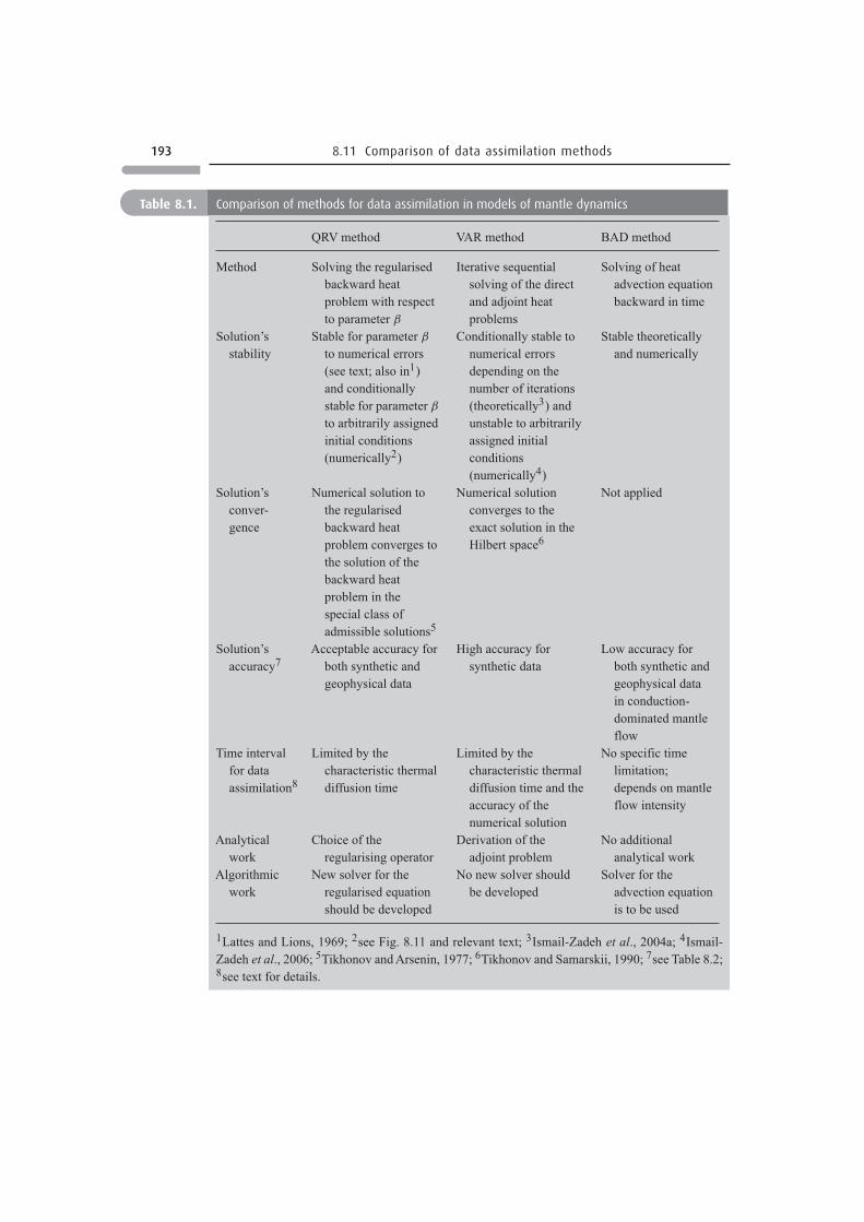
193 8.11 Comparison of data assimilation methods
Table 8.1. Comparison of methods for data assimilation in models of mantle dynamics
QRV method VAR method BAD method
Method Solving the regularisedbackward heatproblem with respectto parameter β
Iterative sequentialsolving of the directand adjoint heatproblems
Solving of heatadvection equationbackward in time
Solution’sstability
Stable for parameter β
to numerical errors(see text; also in1)and conditionallystable for parameter β
to arbitrarily assignedinitial conditions(numerically2)
Conditionally stable tonumerical errorsdepending on thenumber of iterations(theoretically3) andunstable to arbitrarilyassigned initialconditions(numerically4)
Stable theoreticallyand numerically
Solution’sconver-gence
Numerical solution tothe regularisedbackward heatproblem converges tothe solution of thebackward heatproblem in thespecial class ofadmissible solutions5
Numerical solutionconverges to theexact solution in theHilbert space6
Not applied
Solution’saccuracy7
Acceptable accuracy forboth synthetic andgeophysical data
High accuracy forsynthetic data
Low accuracy forboth synthetic andgeophysical datain conduction-dominated mantleflow
Time intervalfor dataassimilation8
Limited by thecharacteristic thermaldiffusion time
Limited by thecharacteristic thermaldiffusion time and theaccuracy of thenumerical solution
No specific timelimitation;depends on mantleflow intensity
Analyticalwork
Choice of theregularising operator
Derivation of theadjoint problem
No additionalanalytical work
Algorithmicwork
New solver for theregularised equationshould be developed
No new solver shouldbe developed
Solver for theadvection equationis to be used
1Lattes and Lions, 1969; 2see Fig. 8.11 and relevant text; 3Ismail-Zadeh et al., 2004a; 4Ismail-Zadeh et al., 2006; 5Tikhonov and Arsenin, 1977; 6Tikhonov and Samarskii, 1990; 7see Table 8.2;8see text for details.
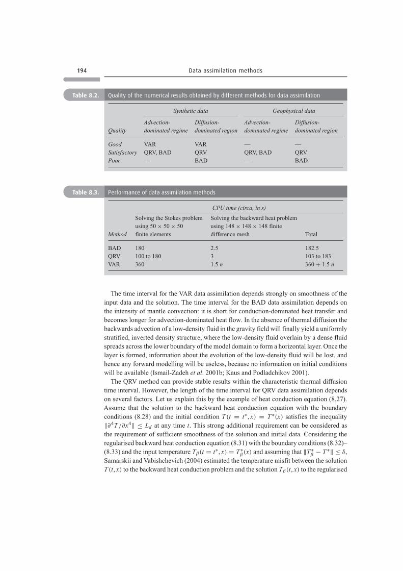
194 Data assimilation methods
Table 8.2. Quality of the numerical results obtained by different methods for data assimilation
Synthetic data Geophysical data
Advection- Diffusion- Advection- Diffusion-Quality dominated regime dominated region dominated regime dominated region
Good VAR VAR — —Satisfactory QRV, BAD QRV QRV, BAD QRVPoor — BAD — BAD
Table 8.3. Performance of data assimilation methods
CPU time (circa, in s)
Solving the Stokes problem Solving the backward heat problemusing 50 × 50 × 50 using 148 × 148 × 148 finite
Method finite elements difference mesh Total
BAD 180 2.5 182.5QRV 100 to 180 3 103 to 183VAR 360 1.5 n 360 + 1.5 n
The time interval for the VAR data assimilation depends strongly on smoothness of theinput data and the solution. The time interval for the BAD data assimilation depends onthe intensity of mantle convection: it is short for conduction-dominated heat transfer andbecomes longer for advection-dominated heat flow. In the absence of thermal diffusion thebackwards advection of a low-density fluid in the gravity field will finally yield a uniformlystratified, inverted density structure, where the low-density fluid overlain by a dense fluidspreads across the lower boundary of the model domain to form a horizontal layer. Once thelayer is formed, information about the evolution of the low-density fluid will be lost, andhence any forward modelling will be useless, because no information on initial conditionswill be available (Ismail-Zadeh et al. 2001b; Kaus and Podladchikov 2001).
The QRV method can provide stable results within the characteristic thermal diffusiontime interval. However, the length of the time interval for QRV data assimilation dependson several factors. Let us explain this by the example of heat conduction equation (8.27).Assume that the solution to the backward heat conduction equation with the boundaryconditions (8.28) and the initial condition T (t = t∗, x) = T ∗(x) satisfies the inequality‖∂4T/∂x4‖ ≤ Ld at any time t. This strong additional requirement can be considered asthe requirement of sufficient smoothness of the solution and initial data. Considering theregularised backward heat conduction equation (8.31) with the boundary conditions (8.32)–(8.33) and the input temperature Tβ(t = t∗, x) = T ∗
β (x) and assuming that ‖T ∗β − T ∗‖ ≤ δ,
Samarskii and Vabishchevich (2004) estimated the temperature misfit between the solutionT (t, x) to the backward heat conduction problem and the solution Tβ(t, x) to the regularised
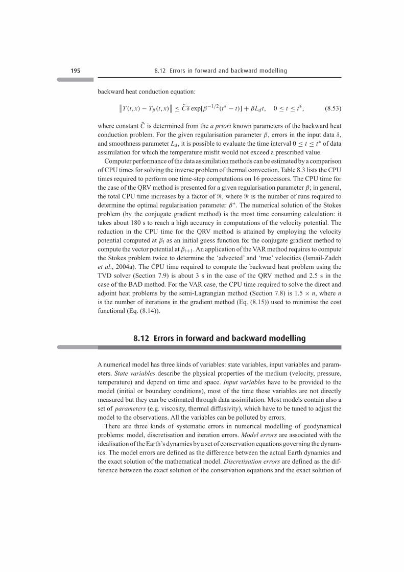
195 8.12 Errors in forward and backward modelling
backward heat conduction equation:
∥∥T (t, x) − Tβ(t, x)∥∥ ≤ C̃δ exp[β−1/2(t∗ − t)] + βLdt, 0 ≤ t ≤ t∗, (8.53)
where constant C̃ is determined from the a priori known parameters of the backward heatconduction problem. For the given regularisation parameter β, errors in the input data δ,and smoothness parameter Ld , it is possible to evaluate the time interval 0 ≤ t ≤ t∗ of dataassimilation for which the temperature misfit would not exceed a prescribed value.
Computer performance of the data assimilation methods can be estimated by a comparisonof CPU times for solving the inverse problem of thermal convection. Table 8.3 lists the CPUtimes required to perform one time-step computations on 16 processors. The CPU time forthe case of the QRV method is presented for a given regularisation parameter β; in general,the total CPU time increases by a factor of , where is the number of runs required todetermine the optimal regularisation parameter β∗. The numerical solution of the Stokesproblem (by the conjugate gradient method) is the most time consuming calculation: ittakes about 180 s to reach a high accuracy in computations of the velocity potential. Thereduction in the CPU time for the QRV method is attained by employing the velocitypotential computed at βi as an initial guess function for the conjugate gradient method tocompute the vector potential at βi+1.An application of the VAR method requires to computethe Stokes problem twice to determine the ‘advected’ and ‘true’ velocities (Ismail-Zadehet al., 2004a). The CPU time required to compute the backward heat problem using theTVD solver (Section 7.9) is about 3 s in the case of the QRV method and 2.5 s in thecase of the BAD method. For the VAR case, the CPU time required to solve the direct andadjoint heat problems by the semi-Lagrangian method (Section 7.8) is 1.5 × n, where nis the number of iterations in the gradient method (Eq. (8.15)) used to minimise the costfunctional (Eq. (8.14)).
8.12 Errors in forward and backward modelling
A numerical model has three kinds of variables: state variables, input variables and param-eters. State variables describe the physical properties of the medium (velocity, pressure,temperature) and depend on time and space. Input variables have to be provided to themodel (initial or boundary conditions), most of the time these variables are not directlymeasured but they can be estimated through data assimilation. Most models contain also aset of parameters (e.g. viscosity, thermal diffusivity), which have to be tuned to adjust themodel to the observations. All the variables can be polluted by errors.
There are three kinds of systematic errors in numerical modelling of geodynamicalproblems: model, discretisation and iteration errors. Model errors are associated with theidealisation of the Earth’s dynamics by a set of conservation equations governing the dynam-ics. The model errors are defined as the difference between the actual Earth dynamics andthe exact solution of the mathematical model. Discretisation errors are defined as the dif-ference between the exact solution of the conservation equations and the exact solution of
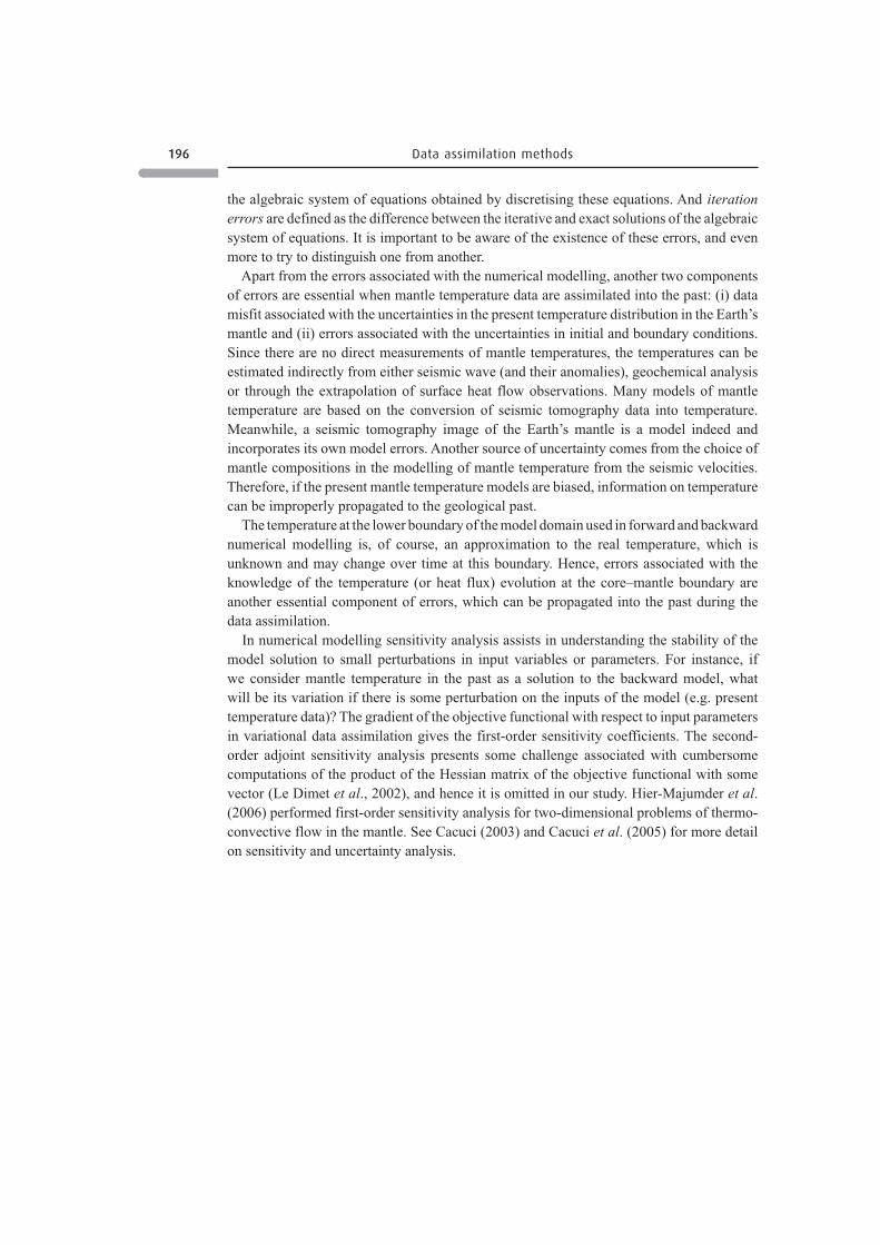
196 Data assimilation methods
the algebraic system of equations obtained by discretising these equations. And iterationerrors are defined as the difference between the iterative and exact solutions of the algebraicsystem of equations. It is important to be aware of the existence of these errors, and evenmore to try to distinguish one from another.
Apart from the errors associated with the numerical modelling, another two componentsof errors are essential when mantle temperature data are assimilated into the past: (i) datamisfit associated with the uncertainties in the present temperature distribution in the Earth’smantle and (ii) errors associated with the uncertainties in initial and boundary conditions.Since there are no direct measurements of mantle temperatures, the temperatures can beestimated indirectly from either seismic wave (and their anomalies), geochemical analysisor through the extrapolation of surface heat flow observations. Many models of mantletemperature are based on the conversion of seismic tomography data into temperature.Meanwhile, a seismic tomography image of the Earth’s mantle is a model indeed andincorporates its own model errors. Another source of uncertainty comes from the choice ofmantle compositions in the modelling of mantle temperature from the seismic velocities.Therefore, if the present mantle temperature models are biased, information on temperaturecan be improperly propagated to the geological past.
The temperature at the lower boundary of the model domain used in forward and backwardnumerical modelling is, of course, an approximation to the real temperature, which isunknown and may change over time at this boundary. Hence, errors associated with theknowledge of the temperature (or heat flux) evolution at the core–mantle boundary areanother essential component of errors, which can be propagated into the past during thedata assimilation.
In numerical modelling sensitivity analysis assists in understanding the stability of themodel solution to small perturbations in input variables or parameters. For instance, ifwe consider mantle temperature in the past as a solution to the backward model, whatwill be its variation if there is some perturbation on the inputs of the model (e.g. presenttemperature data)? The gradient of the objective functional with respect to input parametersin variational data assimilation gives the first-order sensitivity coefficients. The second-order adjoint sensitivity analysis presents some challenge associated with cumbersomecomputations of the product of the Hessian matrix of the objective functional with somevector (Le Dimet et al., 2002), and hence it is omitted in our study. Hier-Majumder et al.(2006) performed first-order sensitivity analysis for two-dimensional problems of thermo-convective flow in the mantle. See Cacuci (2003) and Cacuci et al. (2005) for more detailon sensitivity and uncertainty analysis.
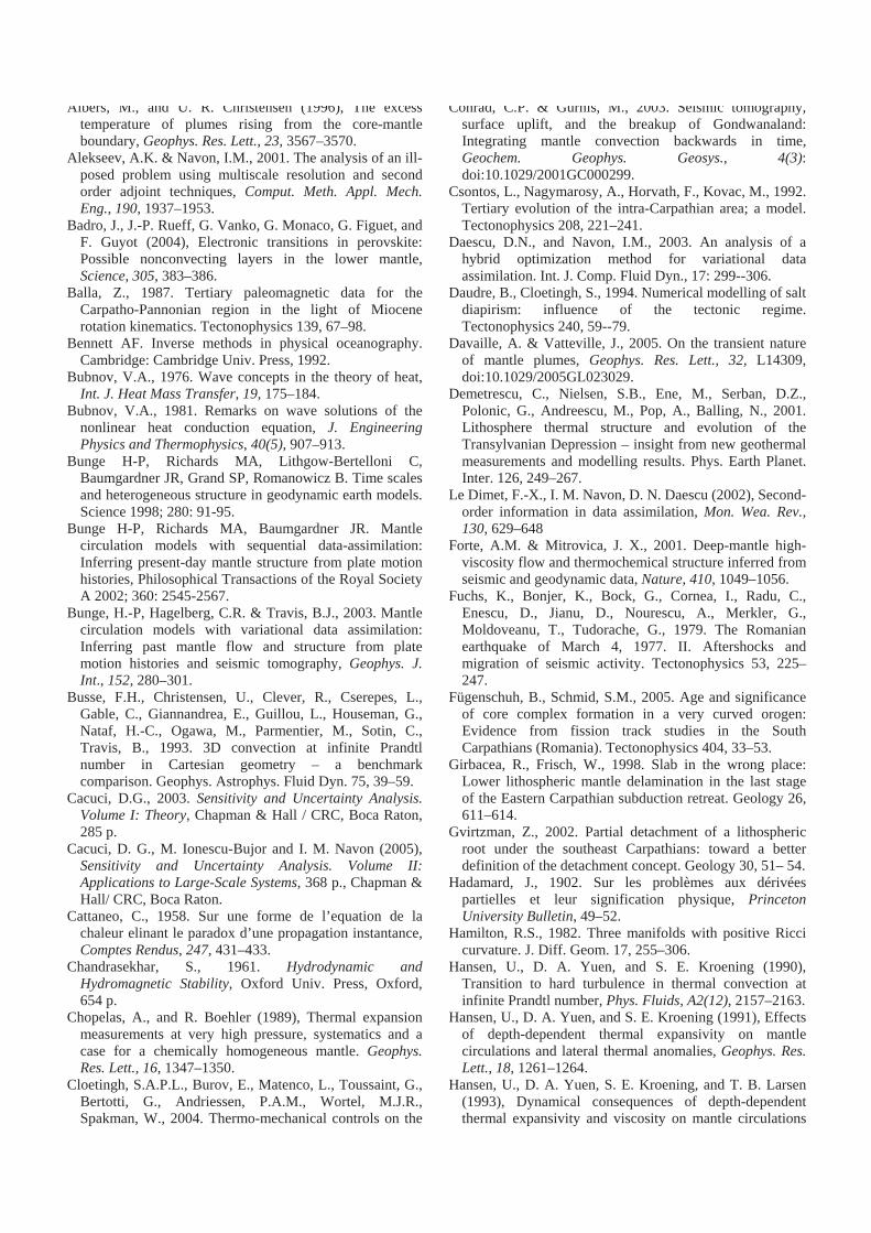
Albers, M., and U. R. Christensen (1996), The excess temperature of plumes rising from the core-mantle boundary, Geophys. Res. Lett., 23, 3567–3570.
Alekseev, A.K. & Navon, I.M., 2001. The analysis of an ill-posed problem using multiscale resolution and second order adjoint techniques, Comput. Meth. Appl. Mech. Eng., 190, 1937–1953.
Badro, J., J.-P. Rueff, G. Vanko, G. Monaco, G. Figuet, and F. Guyot (2004), Electronic transitions in perovskite: Possible nonconvecting layers in the lower mantle, Science, 305, 383–386.
Balla, Z., 1987. Tertiary paleomagnetic data for the Carpatho-Pannonian region in the light of Miocene rotation kinematics. Tectonophysics 139, 67–98.
Bennett AF. Inverse methods in physical oceanography. Cambridge: Cambridge Univ. Press, 1992.
Bubnov, V.A., 1976. Wave concepts in the theory of heat, Int. J. Heat Mass Transfer, 19, 175–184.
Bubnov, V.A., 1981. Remarks on wave solutions of the nonlinear heat conduction equation, J. Engineering Physics and Thermophysics, 40(5), 907–913.
Bunge H-P, Richards MA, Lithgow-Bertelloni C, Baumgardner JR, Grand SP, Romanowicz B. Time scales and heterogeneous structure in geodynamic earth models. Science 1998; 280: 91-95.
Bunge H-P, Richards MA, Baumgardner JR. Mantle circulation models with sequential data-assimilation: Inferring present-day mantle structure from plate motion histories, Philosophical Transactions of the Royal Society A 2002; 360: 2545-2567.
Bunge, H.-P, Hagelberg, C.R. & Travis, B.J., 2003. Mantle circulation models with variational data assimilation: Inferring past mantle flow and structure from plate motion histories and seismic tomography, Geophys. J. Int., 152, 280–301.
Busse, F.H., Christensen, U., Clever, R., Cserepes, L., Gable, C., Giannandrea, E., Guillou, L., Houseman, G., Nataf, H.-C., Ogawa, M., Parmentier, M., Sotin, C., Travis, B., 1993. 3D convection at infinite Prandtl number in Cartesian geometry – a benchmark comparison. Geophys. Astrophys. Fluid Dyn. 75, 39–59.
Cacuci, D.G., 2003. Sensitivity and Uncertainty Analysis. Volume I: Theory, Chapman & Hall / CRC, Boca Raton, 285 p.
Cacuci, D. G., M. Ionescu-Bujor and I. M. Navon (2005), Sensitivity and Uncertainty Analysis. Volume II: Applications to Large-Scale Systems, 368 p., Chapman & Hall/ CRC, Boca Raton.
Cattaneo, C., 1958. Sur une forme de l’equation de la chaleur elinant le paradox d’une propagation instantance, Comptes Rendus, 247, 431–433.
Chandrasekhar, S., 1961. Hydrodynamic and Hydromagnetic Stability, Oxford Univ. Press, Oxford, 654 p.
Chopelas, A., and R. Boehler (1989), Thermal expansion measurements at very high pressure, systematics and a case for a chemically homogeneous mantle. Geophys.Res. Lett., 16, 1347–1350.
Cloetingh, S.A.P.L., Burov, E., Matenco, L., Toussaint, G., Bertotti, G., Andriessen, P.A.M., Wortel, M.J.R., Spakman, W., 2004. Thermo-mechanical controls on the
Conrad, C.P. & Gurnis, M., 2003. Seismic tomography, surface uplift, and the breakup of Gondwanaland: Integrating mantle convection backwards in time, Geochem. Geophys. Geosys., 4(3):doi:10.1029/2001GC000299.
Csontos, L., Nagymarosy, A., Horvath, F., Kovac, M., 1992. Tertiary evolution of the intra-Carpathian area; a model. Tectonophysics 208, 221–241.
Daescu, D.N., and Navon, I.M., 2003. An analysis of a hybrid optimization method for variational data assimilation. Int. J. Comp. Fluid Dyn., 17: 299--306.
Daudre, B., Cloetingh, S., 1994. Numerical modelling of salt diapirism: influence of the tectonic regime. Tectonophysics 240, 59--79.
Davaille, A. & Vatteville, J., 2005. On the transient nature of mantle plumes, Geophys. Res. Lett., 32, L14309, doi:10.1029/2005GL023029.
Demetrescu, C., Nielsen, S.B., Ene, M., Serban, D.Z., Polonic, G., Andreescu, M., Pop, A., Balling, N., 2001. Lithosphere thermal structure and evolution of the Transylvanian Depression – insight from new geothermal measurements and modelling results. Phys. Earth Planet. Inter. 126, 249–267.
Le Dimet, F.-X., I. M. Navon, D. N. Daescu (2002), Second-order information in data assimilation, Mon. Wea. Rev., 130, 629–648
Forte, A.M. & Mitrovica, J. X., 2001. Deep-mantle high-viscosity flow and thermochemical structure inferred from seismic and geodynamic data, Nature, 410, 1049–1056.
Fuchs, K., Bonjer, K., Bock, G., Cornea, I., Radu, C., Enescu, D., Jianu, D., Nourescu, A., Merkler, G., Moldoveanu, T., Tudorache, G., 1979. The Romanian earthquake of March 4, 1977. II. Aftershocks and migration of seismic activity. Tectonophysics 53, 225–247.
Fügenschuh, B., Schmid, S.M., 2005. Age and significance of core complex formation in a very curved orogen: Evidence from fission track studies in the South Carpathians (Romania). Tectonophysics 404, 33–53.
Girbacea, R., Frisch, W., 1998. Slab in the wrong place: Lower lithospheric mantle delamination in the last stage of the Eastern Carpathian subduction retreat. Geology 26, 611–614.
Gvirtzman, Z., 2002. Partial detachment of a lithospheric root under the southeast Carpathians: toward a better definition of the detachment concept. Geology 30, 51– 54.
Hadamard, J., 1902. Sur les problèmes aux dérivées partielles et leur signification physique, PrincetonUniversity Bulletin, 49–52.
Hamilton, R.S., 1982. Three manifolds with positive Ricci curvature. J. Diff. Geom. 17, 255–306.
Hansen, U., D. A. Yuen, and S. E. Kroening (1990), Transition to hard turbulence in thermal convection at infinite Prandtl number, Phys. Fluids, A2(12), 2157–2163.
Hansen, U., D. A. Yuen, and S. E. Kroening (1991), Effects of depth-dependent thermal expansivity on mantle circulations and lateral thermal anomalies, Geophys. Res. Lett., 18, 1261–1264.
Hansen, U., D. A. Yuen, S. E. Kroening, and T. B. Larsen (1993), Dynamical consequences of depth-dependent thermal expansivity and viscosity on mantle circulations
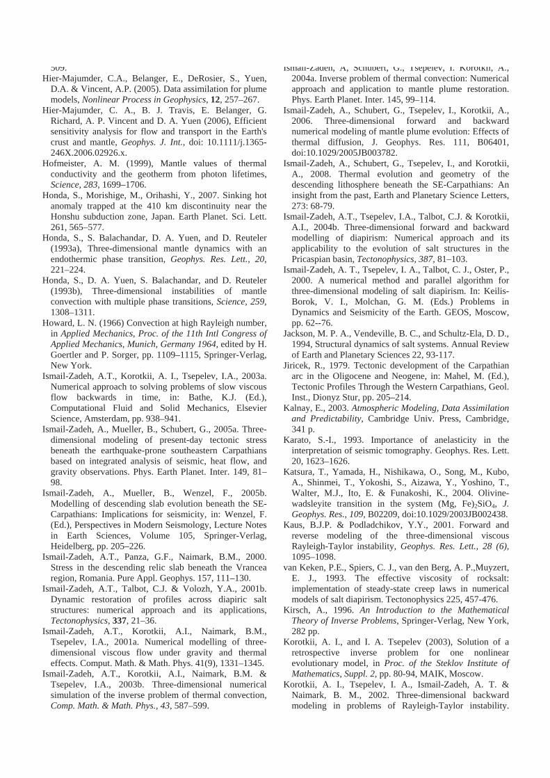
509.Hier-Majumder, C.A., Belanger, E., DeRosier, S., Yuen,
D.A. & Vincent, A.P. (2005). Data assimilation for plume models, Nonlinear Process in Geophysics, 12, 257–267.
Hier-Majumder, C. A., B. J. Travis, E. Belanger, G. Richard, A. P. Vincent and D. A. Yuen (2006), Efficient sensitivity analysis for flow and transport in the Earth's crust and mantle, Geophys. J. Int., doi: 10.1111/j.1365-246X.2006.02926.x.
Hofmeister, A. M. (1999), Mantle values of thermal conductivity and the geotherm from photon lifetimes, Science, 283, 1699–1706.
Honda, S., Morishige, M., Orihashi, Y., 2007. Sinking hot anomaly trapped at the 410 km discontinuity near the Honshu subduction zone, Japan. Earth Planet. Sci. Lett. 261, 565–577.
Honda, S., S. Balachandar, D. A. Yuen, and D. Reuteler (1993a), Three-dimensional mantle dynamics with an endothermic phase transition, Geophys. Res. Lett., 20,221–224.
Honda, S., D. A. Yuen, S. Balachandar, and D. Reuteler (1993b), Three-dimensional instabilities of mantle convection with multiple phase transitions, Science, 259,1308–1311.
Howard, L. N. (1966) Convection at high Rayleigh number, in Applied Mechanics, Proc. of the 11th Intl Congress of Applied Mechanics, Munich, Germany 1964, edited by H. Goertler and P. Sorger, pp. 1109–1115, Springer-Verlag, New York.
Ismail-Zadeh, A.T., Korotkii, A. I., Tsepelev, I.A., 2003a. Numerical approach to solving problems of slow viscous flow backwards in time, in: Bathe, K.J. (Ed.), Computational Fluid and Solid Mechanics, Elsevier Science, Amsterdam, pp. 938–941.
Ismail-Zadeh, A., Mueller, B., Schubert, G., 2005a. Three-dimensional modeling of present-day tectonic stress beneath the earthquake-prone southeastern Carpathians based on integrated analysis of seismic, heat flow, and gravity observations. Phys. Earth Planet. Inter. 149, 81–98.
Ismail-Zadeh, A., Mueller, B., Wenzel, F., 2005b. Modelling of descending slab evolution beneath the SE-Carpathians: Implications for seismicity, in: Wenzel, F. (Ed.), Perspectives in Modern Seismology, Lecture Notes in Earth Sciences, Volume 105, Springer-Verlag, Heidelberg, pp. 205–226.
Ismail-Zadeh, A.T., Panza, G.F., Naimark, B.M., 2000. Stress in the descending relic slab beneath the Vrancea region, Romania. Pure Appl. Geophys. 157, 111–130.
Ismail-Zadeh, A.T., Talbot, C.J. & Volozh, Y.A., 2001b. Dynamic restoration of profiles across diapiric salt structures: numerical approach and its applications, Tectonophysics, 337, 21–36.
Ismail-Zadeh, A.T., Korotkii, A.I., Naimark, B.M., Tsepelev, I.A., 2001a. Numerical modelling of three-dimensional viscous flow under gravity and thermal effects. Comput. Math. & Math. Phys. 41(9), 1331–1345.
Ismail-Zadeh, A.T., Korotkii, A.I., Naimark, B.M. & Tsepelev, I.A., 2003b. Three-dimensional numerical simulation of the inverse problem of thermal convection, Comp. Math. & Math. Phys., 43, 587–599.
Ismail-Zadeh, A, Schubert, G., Tsepelev, I. Korotkii, A., 2004a. Inverse problem of thermal convection: Numerical approach and application to mantle plume restoration. Phys. Earth Planet. Inter. 145, 99–114.
Ismail-Zadeh, A., Schubert, G., Tsepelev, I., Korotkii, A., 2006. Three-dimensional forward and backward numerical modeling of mantle plume evolution: Effects of thermal diffusion, J. Geophys. Res. 111, B06401, doi:10.1029/2005JB003782.
Ismail-Zadeh, A., Schubert, G., Tsepelev, I., and Korotkii, A., 2008. Thermal evolution and geometry of the descending lithosphere beneath the SE-Carpathians: An insight from the past, Earth and Planetary Science Letters,273: 68-79.
Ismail-Zadeh, A.T., Tsepelev, I.A., Talbot, C.J. & Korotkii, A.I., 2004b. Three-dimensional forward and backward modelling of diapirism: Numerical approach and its applicability to the evolution of salt structures in the Pricaspian basin, Tectonophysics, 387, 81–103.
Ismail-Zadeh, A. T., Tsepelev, I. A., Talbot, C. J., Oster, P., 2000. A numerical method and parallel algorithm for three-dimensional modeling of salt diapirism. In: Keilis-Borok, V. I., Molchan, G. M. (Eds.) Problems in Dynamics and Seismicity of the Earth. GEOS, Moscow, pp. 62--76.
Jackson, M. P. A., Vendeville, B. C., and Schultz-Ela, D. D., 1994, Structural dynamics of salt systems. Annual Review of Earth and Planetary Sciences 22, 93-117.
Jiricek, R., 1979. Tectonic development of the Carpathian arc in the Oligocene and Neogene, in: Mahel, M. (Ed.), Tectonic Profiles Through the Western Carpathians, Geol. Inst., Dionyz Stur, pp. 205–214.
Kalnay, E., 2003. Atmospheric Modeling, Data Assimilation and Predictability, Cambridge Univ. Press, Cambridge, 341 p.
Karato, S.-I., 1993. Importance of anelasticity in the interpretation of seismic tomography. Geophys. Res. Lett. 20, 1623–1626.
Katsura, T., Yamada, H., Nishikawa, O., Song, M., Kubo, A., Shinmei, T., Yokoshi, S., Aizawa, Y., Yoshino, T., Walter, M.J., Ito, E. & Funakoshi, K., 2004. Olivine-wadsleyite transition in the system (Mg, Fe)2SiO4, J.Geophys. Res., 109, B02209, doi:10.1029/2003JB002438.
Kaus, B.J.P. & Podladchikov, Y.Y., 2001. Forward and reverse modeling of the three-dimensional viscous Rayleigh-Taylor instability, Geophys. Res. Lett., 28 (6),1095–1098.
van Keken, P.E., Spiers, C. J., van den Berg, A. P.,Muyzert, E. J., 1993. The effective viscosity of rocksalt: implementation of steady-state creep laws in numerical models of salt diapirism. Tectonophysics 225, 457-476.
Kirsch, A., 1996. An Introduction to the Mathematical Theory of Inverse Problems, Springer-Verlag, New York, 282 pp.
Korotkii, A. I., and I. A. Tsepelev (2003), Solution of a retrospective inverse problem for one nonlinear evolutionary model, in Proc. of the Steklov Institute of Mathematics, Suppl. 2, pp. 80-94, MAIK, Moscow.
Korotkii, A. I., Tsepelev, I. A., Ismail-Zadeh, A. T. & Naimark, B. M., 2002. Three-dimensional backward modeling in problems of Rayleigh-Taylor instability.
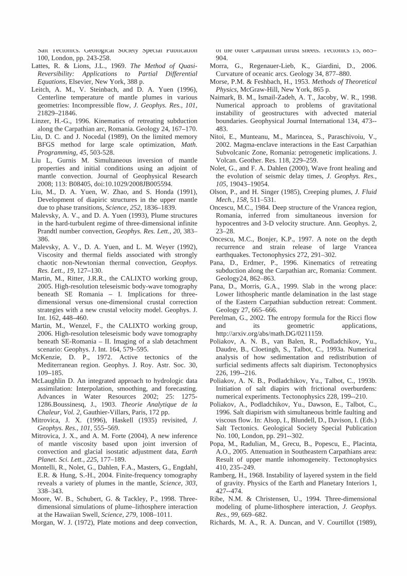
Salt Tectonics. Geological Society Special Publication 100, London, pp. 243-258.
Lattes, R. & Lions, J.L., 1969. The Method of Quasi-Reversibility: Applications to Partial Differential Equations, Elsevier, New York, 388 p.
Leitch, A. M., V. Steinbach, and D. A. Yuen (1996), Centerline temperature of mantle plumes in various geometries: Incompressible flow, J. Geophys. Res., 101,21829–21846.
Linzer, H.-G., 1996. Kinematics of retreating subduction along the Carpathian arc, Romania. Geology 24, 167–170.
Liu, D. C. and J. Nocedal (1989), On the limited memory BFGS method for large scale optimization, Math.Programming, 45, 503-528.
Liu L, Gurnis M. Simultaneous inversion of mantle properties and initial conditions using an adjoint of mantle convection. Journal of Geophysical Research 2008; 113: B08405, doi:10.1029/2008JB005594.
Liu, M., D. A. Yuen, W. Zhao, and S. Honda (1991), Development of diapiric structures in the upper mantle due to phase transitions, Science, 252, 1836–1839.
Malevsky, A. V., and D. A. Yuen (1993), Plume structures in the hard-turbulent regime of three-dimensional infinite Prandtl number convection, Geophys. Res. Lett., 20, 383–386.
Malevsky, A. V., D. A. Yuen, and L. M. Weyer (1992), Viscosity and thermal fields associated with strongly chaotic non-Newtonian thermal convection, Geophys.Res. Lett., 19, 127–130.
Martin, M., Ritter, J.R.R., the CALIXTO working group, 2005. High-resolution teleseismic body-wave tomography beneath SE Romania – I. Implications for three-dimensional versus one-dimensional crustal correction strategies with a new crustal velocity model. Geophys. J. Int. 162, 448–460.
Martin, M., Wenzel, F., the CALIXTO working group, 2006. High-resolution teleseismic body wave tomography beneath SE-Romania – II. Imaging of a slab detachment scenario: Geophys. J. Int. 164, 579–595.
McKenzie, D. P., 1972. Active tectonics of the Mediterranean region. Geophys. J. Roy. Astr. Soc. 30, 109–185.
McLaughlin D. An integrated approach to hydrologic data assimilation: Interpolation, smoothing, and forecasting. Advances in Water Resources 2002; 25: 1275-1286.Boussinesq, J., 1903. Theorie Analytique de la Chaleur, Vol. 2, Gauthier-Villars, Paris, 172 pp.
Mitrovica, J. X. (1996), Haskell (1935) revisited, J.Geophys. Res., 101, 555–569.
Mitrovica, J. X., and A. M. Forte (2004), A new inference of mantle viscosity based upon joint inversion of convection and glacial isostatic adjustment data, EarthPlanet. Sci. Lett., 225, 177–189.
Montelli, R., Nolet, G., Dahlen, F.A., Masters, G., Engdahl, E.R. & Hung, S.-H., 2004. Finite-frequency tomography reveals a variety of plumes in the mantle, Science, 303,338–343.
Moore, W. B., Schubert, G. & Tackley, P., 1998. Three-dimensional simulations of plume–lithosphere interaction at the Hawaiian Swell, Science, 279, 1008–1011.
Morgan, W. J. (1972), Plate motions and deep convection,
of the outer Carpathian thrust sheets. Tectonics 15, 885–904.
Morra, G., Regenauer-Lieb, K., Giardini, D., 2006. Curvature of oceanic arcs. Geology 34, 877–880.
Morse, P.M. & Feshbach, H., 1953. Methods of Theoretical Physics, McGraw-Hill, New York, 865 p.
Naimark, B. M., Ismail-Zadeh, A. T., Jacoby, W. R., 1998. Numerical approach to problems of gravitational instability of geostructures with advected material boundaries. Geophysical Journal International 134, 473--483.
Nitoi, E., Munteanu, M., Marincea, S., Paraschivoiu, V., 2002. Magma-enclave interactions in the East Carpathian Subvolcanic Zone, Romania: petrogenetic implications. J. Volcan. Geother. Res. 118, 229–259.
Nolet, G., and F. A. Dahlen (2000), Wave front healing and the evolution of seismic delay times, J. Geophys. Res., 105, 19043–19054.
Olson, P., and H. Singer (1985), Creeping plumes, J. Fluid Mech., 158, 511–531.
Oncescu, M.C., 1984. Deep structure of the Vrancea region, Romania, inferred from simultaneous inversion for hypocentres and 3-D velocity structure. Ann. Geophys. 2, 23–28.
Oncescu, M.C., Bonjer, K.P., 1997. A note on the depth recurrence and strain release of large Vrancea earthquakes. Tectonophysics 272, 291–302.
Pana, D., Erdmer, P., 1996. Kinematics of retreating subduction along the Carpathian arc, Romania: Comment. Geology24, 862–863.
Pana, D., Morris, G.A., 1999. Slab in the wrong place: Lower lithospheric mantle delamination in the last stage of the Eastern Carpathian subduction retreat: Comment. Geology 27, 665–666.
Perelman, G., 2002. The entropy formula for the Ricci flow and its geometric applications, http://arxiv.org/abs/math.DG/0211159.
Poliakov, A. N. B., van Balen, R., Podladchikov, Yu., Daudre, B., Cloetingh, S., Talbot, C., 1993a. Numerical analysis of how sedimentation and redistribution of surficial sediments affects salt diapirism. Tectonophysics 226, 199--216.
Poliakov, A. N. B., Podladchikov, Yu., Talbot, C., 1993b. Initiation of salt diapirs with frictional overburdens: numerical experiments. Tectonophysics 228, 199--210.
Poliakov, A., Podladchikov, Yu., Dawson, E., Talbot, C., 1996. Salt diapirism with simultaneous brittle faulting and viscous flow. In: Alsop, I., Blundell, D., Davison, I. (Eds.) Salt Tectonics. Geological Society Special Publication No. 100, London, pp. 291--302.
Popa, M., Radulian, M., Grecu, B., Popescu, E., Placinta, A.O., 2005. Attenuation in Southeastern Carpathians area: Result of upper mantle inhomogeneity. Tectonophysics 410, 235–249.
Ramberg, H., 1968. Instability of layered system in the field of gravity. Physics of the Earth and Planetary Interiors 1, 427--474.
Ribe, N.M. & Christensen, U., 1994. Three-dimensional modeling of plume-lithosphere interaction, J. Geophys. Res., 99, 669–682.
Richards, M. A., R. A. Duncan, and V. Courtillot (1989),
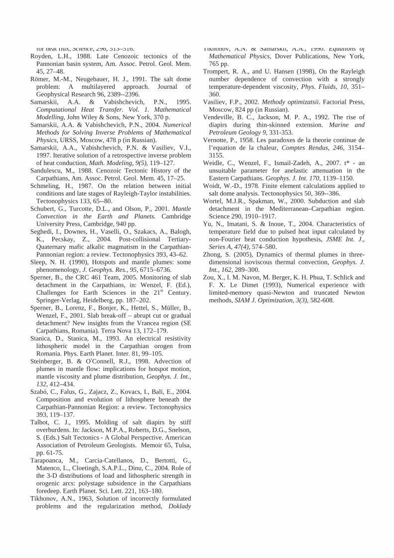
for heat flux, Science, 296, 513–516. Royden, L.H., 1988. Late Cenozoic tectonics of the
Pannonian basin system, Am. Assoc. Petrol. Geol. Mem. 45, 27–48.
Römer, M.-M., Neugebauer, H. J., 1991. The salt dome problem: A multilayered approach. Journal of Geophysical Research 96, 2389--2396.
Samarskii, A.A. & Vabishchevich, P.N., 1995. Computational Heat Transfer. Vol. 1. Mathematical Modelling, John Wiley & Sons, New York, 370 p.
Samarskii, A.A. & Vabishchevich, P.N., 2004. Numerical Methods for Solving Inverse Problems of Mathematical Physics, URSS, Moscow, 478 p (in Russian).
Samarskii, A.A., Vabishchevich, P.N. & Vasiliev, V.I., 1997. Iterative solution of a retrospective inverse problem of heat conduction, Math. Modeling, 9(5), 119–127.
Sandulescu, M., 1988. Cenozoic Tectonic History of the Carpathians, Am. Assoc. Petrol. Geol. Mem. 45, 17–25.
Schmeling, H., 1987. On the relation between initial conditions and late stages of Rayleigh-Taylor instabilities. Tectonophysics 133, 65--80.
Schubert, G., Turcotte, D.L., and Olson, P., 2001. Mantle Convection in the Earth and Planets. Cambridge University Press, Cambridge, 940 pp.
Seghedi, I., Downes, H., Vaselli, O., Szakacs, A., Balogh, K., Pecskay, Z., 2004. Post-collisional Tertiary-Quaternary mafic alkalic magmatism in the Carpathian-Pannonian region: a review. Tectonophysics 393, 43–62.
Sleep, N. H. (1990), Hotspots and mantle plumes: some phenomenology, J. Geophys. Res., 95, 6715–6736.
Sperner, B., the CRC 461 Team, 2005. Monitoring of slab detachment in the Carpathians, in: Wenzel, F. (Ed.), Challenges for Earth Sciences in the 21st Century. Springer-Verlag, Heidelberg, pp. 187–202.
Sperner, B., Lorenz, F., Bonjer, K., Hettel, S., Müller, B., Wenzel, F., 2001. Slab break-off – abrupt cut or gradual detachment? New insights from the Vrancea region (SE Carpathians, Romania). Terra Nova 13, 172–179.
Stanica, D., Stanica, M., 1993. An electrical resistivity lithospheric model in the Carpathian orogen from Romania. Phys. Earth Planet. Inter. 81, 99–105.
Steinberger, B. & O’Connell, R.J., 1998. Advection of plumes in mantle flow: implications for hotspot motion, mantle viscosity and plume distribution, Geophys. J. Int., 132, 412–434.
Szabó, C., Falus, G., Zajacz, Z., Kovacs, I., Bali, E., 2004. Composition and evolution of lithosphere beneath the Carpathian-Pannonian Region: a review. Tectonophysics 393, 119–137.
Talbot, C. J., 1995. Molding of salt diapirs by stiff overburdens. In: Jackson, M.P.A., Roberts, D.G., Snelson, S. (Eds.) Salt Tectonics - A Global Perspective. American Association of Petroleum Geologists. Memoir 65, Tulsa, pp. 61-75.
Tarapoanca, M., Carcia-Catellanos, D., Bertotti, G., Matenco, L., Cloetingh, S.A.P.L., Dinu, C., 2004. Role of the 3-D distributions of load and lithospheric strength in orogenic arcs: polystage subsidence in the Carpathians foredeep. Earth Planet. Sci. Lett. 221, 163–180.
Tikhonov, A.N., 1963, Solution of incorrectly formulated problems and the regularization method, Doklady
Tikhonov, A.N. & Samarskii, A.A., 1990. Equations of Mathematical Physics, Dover Publications, New York, 765 pp.
Trompert, R. A., and U. Hansen (1998), On the Rayleigh number dependence of convection with a strongly temperature-dependent viscosity, Phys. Fluids, 10, 351–360.
Vasiliev, F.P., 2002. Methody optimizatsii. Factorial Press, Moscow, 824 pp (in Russian).
Vendeville, B. C., Jackson, M. P. A., 1992. The rise of diapirs during thin-skinned extension. Marine and Petroleum Geology 9, 331-353.
Vernotte, P., 1958. Les paradoxes de la theorie continue de l’equation de la chaleur, Comptes Rendus, 246, 3154–3155.
Weidle, C., Wenzel, F., Ismail-Zadeh, A., 2007. t* - an unsuitable parameter for anelastic attenuation in the Eastern Carpathians. Geophys. J. Int. 170, 1139–1150.
Woidt, W.-D., 1978. Finite element calculations applied to salt dome analysis. Tectonophysics 50, 369--386.
Wortel, M.J.R., Spakman, W., 2000. Subduction and slab detachment in the Mediterranean–Carpathian region. Science 290, 1910–1917.
Yu, N., Imatani, S. & Inoue, T., 2004. Characteristics of temperature field due to pulsed heat input calculated by non-Fourier heat conduction hypothesis, JSME Int. J., Series A, 47(4), 574–580.
Zhong, S. (2005), Dynamics of thermal plumes in three-dimensional isoviscous thermal convection, Geophys. J. Int., 162, 289–300.
Zou, X., I. M. Navon, M. Berger, K. H. Phua, T. Schlick and F. X. Le Dimet (1993), Numerical experience with limited-memory quasi-Newton and truncated Newton methods, SIAM J. Optimization, 3(3), 582-608.