Workplace Project Portfolio C (WPP C)

1

Workplace Project Portfolio C (WPP C)

Scott A Sims

Front sheet

1. Project title

Factors associated with duration of breastmilk provision to children during the

first six months: a national perspective.

2. Location and dates

This project used data from the 2010 Australian National Infant Feeding Survey

conducted by the Australian Institute of Health and Welfare (AIHW). The

analyses were conducted between July and November 2011.

3. Context

The Infant Feeding Survey is one of the few surveys run entirely by the AIHW.

In this regard it allowed easy access to the data and provided an opportunity

for myself (as a senior data analyst at the AIHW) to conduct further analysis on

the survey data that was not initially budgeted for. This subject area is also of

great interest to me, especially having a 20 month old daughter of my own.

The primary objective of the project was to determine the factors that

contributed to the length of time mothers spent breastfeeding their child (a

longer duration equates to higher breast feeding success), with particular

interest in the effect of pacifier use.

4. Contribution of student to the project as a whole

• Deriving the research topic

• Obtaining data

• Data had already been cleaned by the AIHW but certain variables

required for analysis needed to be derived.

• Formatting and labelling data

• Selecting appropriate methodology suitable for analysing data

• Setting up data for survival analysis

• Building model and validating assumptions

2

• Analysing and reporting of results

5. Statistical issues involved

• Treatment of missing data

• Treatment of outliers

• Validating proportional hazards assumption

• Overall goodness of fit of the model

6. Signed declaration by student

I declare this project is evidence of my own work, with direction and assistance

provided by my project supervisors. This work has not been previously

submitted for academic credit.

………………………………………. ……………………………………….

Scott A Sims Date

Supervisor Statement

I confirm that Scott did indeed contribute to the project as he has stated above.

This was not a straightforward modelling exercise and I believe Scott has

learned a great deal from doing this project; in particular, about dealing with

collinearity and apparent violations of the proportional hazards assumption in

a large data set with many variables, and also about presentation and

discussion of results. He worked diligently on repeated iterations of the

analysis and was very tolerant of some long delays in replying by his

supervisor!

………………………………………. ……………………………………….

Judy M Simpson Date

3

Preface

Student’s role

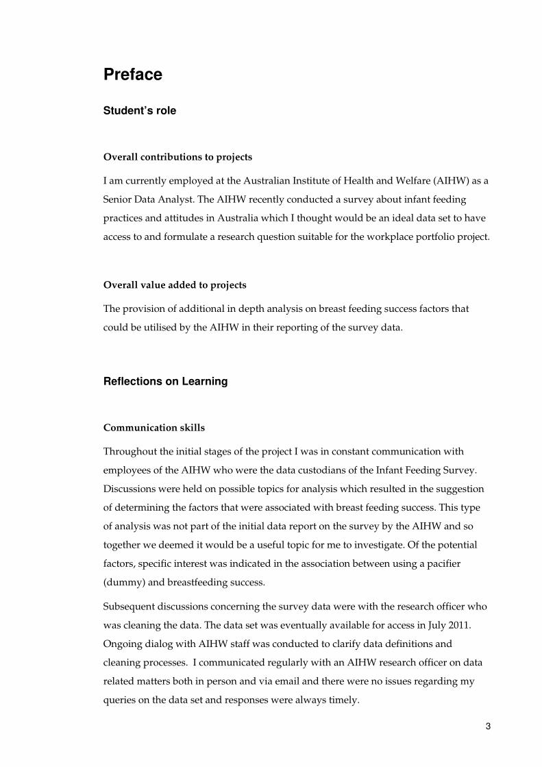
Overall contributions to projects

I am currently employed at the Australian Institute of Health and Welfare (AIHW) as a

Senior Data Analyst. The AIHW recently conducted a survey about infant feeding

practices and attitudes in Australia which I thought would be an ideal data set to have

access to and formulate a research question suitable for the workplace portfolio project.

Overall value added to projects

The provision of additional in depth analysis on breast feeding success factors that

could be utilised by the AIHW in their reporting of the survey data.

Reflections on Learning

Communication skills

Throughout the initial stages of the project I was in constant communication with

employees of the AIHW who were the data custodians of the Infant Feeding Survey.

Discussions were held on possible topics for analysis which resulted in the suggestion

of determining the factors that were associated with breast feeding success. This type

of analysis was not part of the initial data report on the survey by the AIHW and so

together we deemed it would be a useful topic for me to investigate. Of the potential

factors, specific interest was indicated in the association between using a pacifier

(dummy) and breastfeeding success.

Subsequent discussions concerning the survey data were with the research officer who

was cleaning the data. The data set was eventually available for access in July 2011.

Ongoing dialog with AIHW staff was conducted to clarify data definitions and

cleaning processes. I communicated regularly with an AIHW research officer on data

related matters both in person and via email and there were no issues regarding my

queries on the data set and responses were always timely.

4

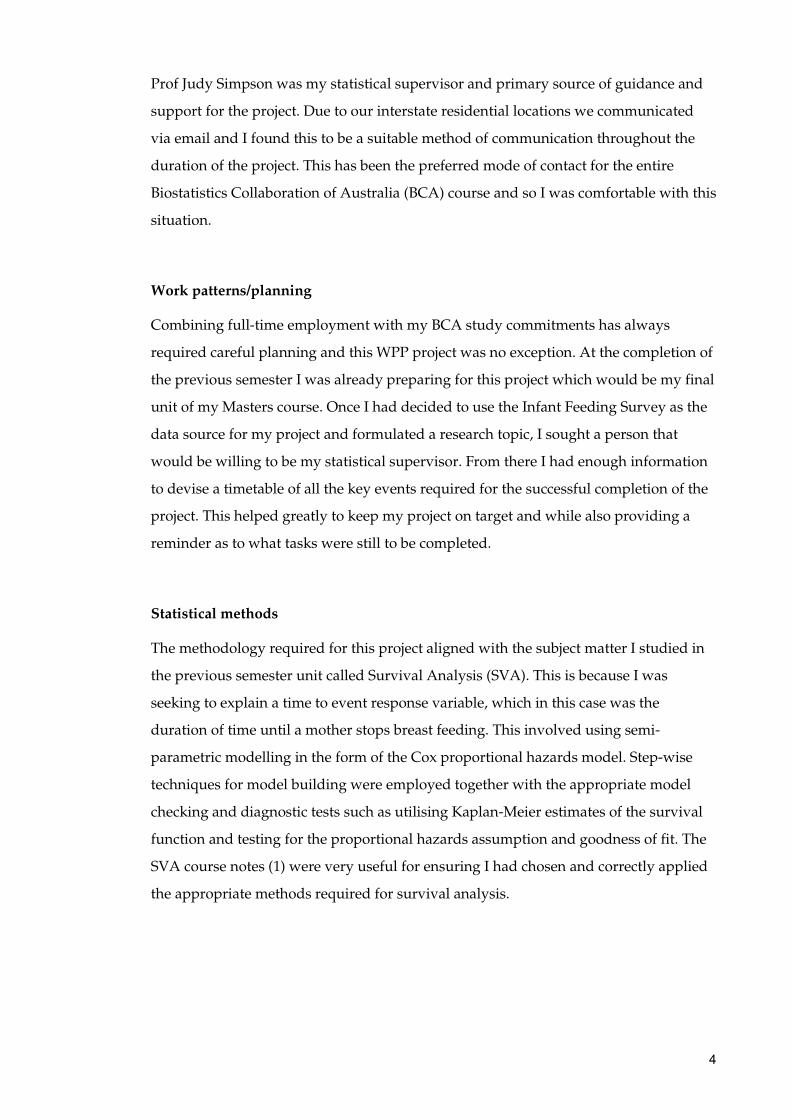
Prof Judy Simpson was my statistical supervisor and primary source of guidance and

support for the project. Due to our interstate residential locations we communicated

via email and I found this to be a suitable method of communication throughout the

duration of the project. This has been the preferred mode of contact for the entire

Biostatistics Collaboration of Australia (BCA) course and so I was comfortable with this

situation.

Work patterns/planning

Combining full-time employment with my BCA study commitments has always

required careful planning and this WPP project was no exception. At the completion of

the previous semester I was already preparing for this project which would be my final

unit of my Masters course. Once I had decided to use the Infant Feeding Survey as the

data source for my project and formulated a research topic, I sought a person that

would be willing to be my statistical supervisor. From there I had enough information

to devise a timetable of all the key events required for the successful completion of the

project. This helped greatly to keep my project on target and while also providing a

reminder as to what tasks were still to be completed.

Statistical methods

The methodology required for this project aligned with the subject matter I studied in

the previous semester unit called Survival Analysis (SVA). This is because I was

seeking to explain a time to event response variable, which in this case was the

duration of time until a mother stops breast feeding. This involved using semi-

parametric modelling in the form of the Cox proportional hazards model. Step-wise

techniques for model building were employed together with the appropriate model

checking and diagnostic tests such as utilising Kaplan-Meier estimates of the survival

function and testing for the proportional hazards assumption and goodness of fit. The

SVA course notes (1) were very useful for ensuring I had chosen and correctly applied

the appropriate methods required for survival analysis.

5

Statistical principles

A number of statistical principles were adhered to during the development of this

project. Censoring and truncation is probably one of the most important concepts that

was taught in the SVA course and was important in understanding the nature of the

survey data as these are typically the main features of survival data. It is where the

outcome is determined to be either missing or all the information on a subject is

missing. If these were not correctly taken into account then it could have invalidated

my analysis. It was also important to understand the concept of survival function

modelling and in particular the functional form for the covariates in the model. For this

project the Cox proportional hazards model (Cox regression) was used which assumes

a functional form for covariates in the model but makes no distributional assumption

about the survival times (as parametric modelling does).

One of the biggest decisions that I had to make regarding the project was the revision

of the scope from investigating duration of breastfeeding for the first 24 months to only

analysing the first six months (censoring those who breast fed longer than 6 months).

This issue arose because of the trouble I was experiencing in getting the final predictive

model to satisfy the proportional hazards assumption. This test consumed a lot of time

and effort and is probably the part of the project that caused the most problems. In

hindsight it is an issue that I could have avoided earlier if I had followed the examples

set by previous studies that usually only investigated the first 6 to 12 months duration

of breastfeeding. Also, in Australia (as well as internationally) it is recommended that

children be exclusively breastfed for the first six months of their life (2). This factor

alone is also what may have resulted in the proportional hazards assumptions being

violated beyond the six month stage as most mothers would be considering stopping

breastfeeding and introducing solid foods.

One of the many benefits of such a lengthy proportional hazards assumption testing

process was that I really understood the reasons behind why we test for the

assumption in the first place and how much of an impact not satisfying the assumption

has on the model results and ability to easily and correctly interpret the outcomes. I

also understood more clearly how important and crucial it is to properly interpret the

Kaplan-Meier curves when exploring the data. I have realised it is a very useful tool in

survival analysis which provides an understanding of the shape of the survival

function for each categorical group and an idea if the groups are proportional or not. It

is this proportionality (where the survival curves are parallel) that I found really useful

as it helped diagnose where the issues with the proportional hazards violation was

6

occurring. In these instances it was clear that the lines were usually converging

approximately after the six month mark which was a catalyst for redefining the scope

of the project.

Statistical computing

Throughout this project I used Stata 10.1 for all data analysis. This was the primary

software used for most of the units in the BCA course and so was the analysis tool I felt

most comfortable using. I used Stata for tasks such as performing extensive data

manipulation, the creation of new variables necessary for survival analysis and

formatting and labelling variables and imputation (e.g. checking for true missing

values and assigning an alternative value otherwise).

One of the most time consuming aspects was preparing the data for survival analysis.

Most of the survey data I had been given access to had been cleaned but there were still

a number of variables that I had to convert from continuous to categorical to remove

outlying effects and skewness. There were also categorical variables that required re-

defining of groups to account for proportional hazard violations. Some groups had to

be combined as they were close to identical in survival rates, while other variables had

to be defined that combined elements of more than one variable to account for multiple

survey questions relating to the same topic.

Correctly defining the time variable was also one of the most important processes and

one which required thorough examination of the sequencing of survey questions that

related to breastfeeding duration. Each one of these questions had to be mapped out in

a flowchart to properly account for all the possible responses that would contribute to

the derivation of duration of breastfeeding.

Teamwork

I consulted with a number of people throughout the duration of this project. These

included two people who were AIHW staff from the Population Health section while

Prof Judy Simpson was my statistical supervisor from the University of Sydney. My

initial point of contact with the data custodians of the AIHW was in May 2011 where

they advised that I could use the Infant Feeding Survey data but that a cleaned version

7

of the data was not yet available. I also met with them several times to discuss that

nature of the data set and what type of analysis would be appropriate.

After the initial discussions that led to the choice of topic for the project and obtaining

the survey data, all the statistical analysis was performed by me under the guidance of

my statistical supervisor. The primary mode of communication within the team was

through email. Ideally having a team all present in the same geographic location would

have been easier and allowed more direct and personal communication but the team

arrangements put in place provided no issues.

To help manage the dispersed nature of the team I found that ongoing communication

was essential to keep my project on schedule. The timetable of key events and targets I

created at the beginning of the project helped greatly with my planning and forced me

to consider the schedules of others and how that would fit into my own plans.

Ethical considerations

Although the data I worked with had already been de-identified, I was not able to use

the survey data outside the AIHW computing environment. This was because of the

confidentiality under which the survey was governed (AIHW Act).

8

Project description

Background

The Australian National Infant Feeding Survey 2010 is the first of its kind in Australia

and is about how Australian mothers and carers feed their children. The health and

wellbeing of children is very important and it is vital that recommended health

measures are in place early in their development.

A large body of Australian and international evidence shows that breastfeeding

provides significant value to children, mothers and society (3) (4). About half of

Australian babies are not receiving any breastmilk by the time they reach six months of

age (5) and those less likely to breastfeed are:

• Aboriginal and Torres Strait Islander mothers

• Less educated mothers of low socio-economic status

• Young mothers.

Reliable national level time trend data and state comparisons for Australian

breastfeeding rates are not available due to inconsistent use of definitions and

methodological differences between surveys (3).

Currently there are no national data available on exclusive breastfeeding for

Indigenous infants or infants in remote or low socio-economic areas.

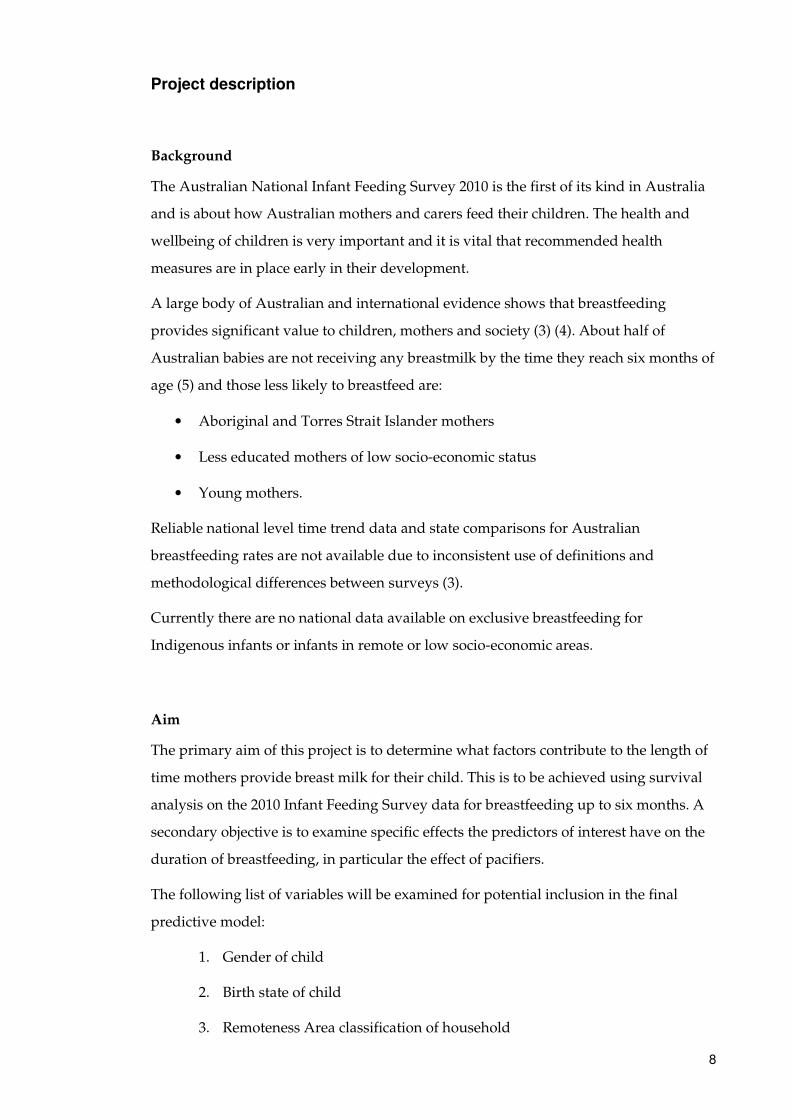
Aim

The primary aim of this project is to determine what factors contribute to the length of

time mothers provide breast milk for their child. This is to be achieved using survival

analysis on the 2010 Infant Feeding Survey data for breastfeeding up to six months. A

secondary objective is to examine specific effects the predictors of interest have on the

duration of breastfeeding, in particular the effect of pacifiers.

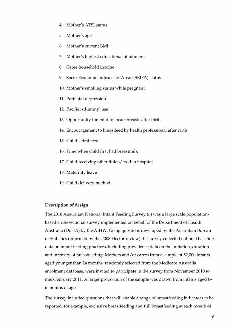
The following list of variables will be examined for potential inclusion in the final

predictive model:

1. Gender of child

2. Birth state of child

3. Remoteness Area classification of household

9

4. Mother’s ATSI status

5. Mother’s age

6. Mother’s current BMI

7. Mother’s highest educational attainment

8. Gross household income

9. Socio-Economic Indexes for Areas (SEIFA) status

10. Mother’s smoking status while pregnant

11. Perinatal depression

12. Pacifier (dummy) use

13. Opportunity for child to locate breasts after birth

14. Encouragement to breastfeed by health professional after birth

15. Child’s first feed

16. Time when child first had breastmilk

17. Child receiving other fluids/food in hospital

18. Maternity leave

19. Child delivery method

Description of design

The 2010 Australian National Infant Feeding Survey (6) was a large scale population-

based cross-sectional survey implemented on behalf of the Department of Health

Australia (DoHA) by the AIHW. Using questions developed by the Australian Bureau

of Statistics (informed by the 2008 Hector review) the survey collected national baseline

data on infant feeding practices, including prevalence data on the initiation, duration

and intensity of breastfeeding. Mothers and/or carers from a sample of 52,000 infants

aged younger than 24 months, randomly selected from the Medicare Australia

enrolment database, were invited to participate in the survey from November 2010 to

mid-February 2011. A larger proportion of the sample was drawn from infants aged 0–

6 months of age.

The survey included questions that will enable a range of breastfeeding indicators to be

reported, for example, exclusive breastfeeding and full breastfeeding at each month of

10

age, and any breastfeeding to 2 years. The outcomes of the survey will also inform

implementation in later years of the Australian National Breastfeeding Strategy 2010–

15 (7) and provide baseline data for strategy evaluation.

Ethical issues

The data obtained for this project were de-identified and hence no risk of identifying

names of people who completed the surveys. I ensured that the data were secure at all

times whilst working on this project by only using the data in a secure environment at

my workplace at the AIHW. The data however still contain sensitive information

which prevents information being released or published by me or any other user of the

data until officially released by the AIHW.

Data management

Obtaining data

The first stage in obtaining access to the survey data was to determine who the data

custodian for the survey was in the AIHW. This was the Head of Population Statistics

at AIHW and so I proceeded to organise a meeting with him to discuss my project idea

and the possibilities of accessing the data required for my project.

A discussion of the survey data took place with the AIHW where they explained what

work had been already done to the data set up to that point and what their intentions

were in terms of analysis and publishing results. The AIHW indicated they would be

happy to provide full access to the final de-identified cleaned data set from the 2010

Australian National Infant Feeding Survey for use with my proposed project.

Subsequent discussions relating to data have been with a research officer at the AIHW

tasked with preparing the data for publication. The research officer supplied a final

version of the cleaned data set in Stata file format in zip form.

The Infant Feeding Survey yielded a response rate of 56% from the random sample of

52,000 mothers and carers selected for the survey. Approximately 28,500 usable records

from this sample were included in the final data set for me to access and analyse. These

records were eventually reduced to 27,190 after manipulating the data into a form that

was suitable for survival analysis and met the scope of this project.

11

Data cleaning

The majority of the data in the version of the survey I received had already been

substantially cleaned with a number of variables already created for the analysis

purposes of the AIHW. However, I still needed to perform some cleaning and data

manipulation to some variables for the purposes of survival analysis. This included

recoding variables, applying out of range rules, and creating composite variables from

pre-existing variables. I had ongoing dialog with the AIHW regarding some of these

data items which included aspects such as seeking clarification of variable definitions

and specifications. I also on occasion was required to remove data for some

respondents when there was key information missing required for survival analysis.

All cleaning/manipulation and analysis were performed using Stata v10.1.

Duration of receiving breastmilk (time)

This data item required cross referencing a number of other survey questions to enable

the most complete data item (as few missing values) as possible.

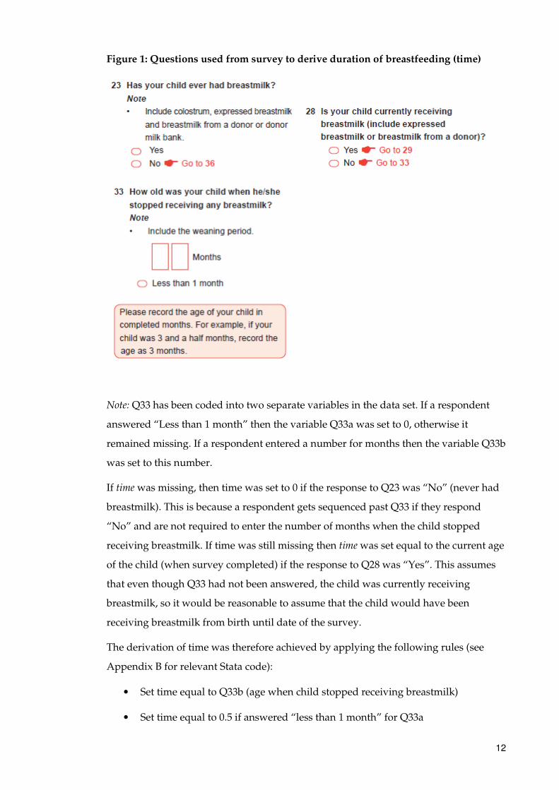
The main source of data for this variable was Q33 of the survey (6), where time was

initially set equal to the response given for Q33 (in months), shown in Figure 1. If the

respondent entered “less than 1 month” the time value was set to 0.5 to ensure those

respondents were set up for survival analysis in the same manner as respondents with

a survival time greater than 1 month (i.e. not treated the same as those with no survival

time or those who were never breastfed).

12

Figure 1: Questions used from survey to derive duration of breastfeeding (time)

Note: Q33 has been coded into two separate variables in the data set. If a respondent

answered “Less than 1 month” then the variable Q33a was set to 0, otherwise it

remained missing. If a respondent entered a number for months then the variable Q33b

was set to this number.

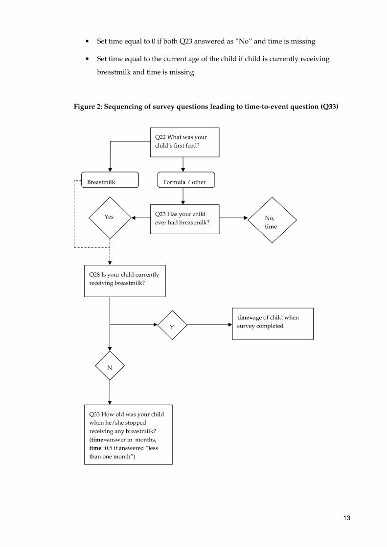
If time was missing, then time was set to 0 if the response to Q23 was “No” (never had

breastmilk). This is because a respondent gets sequenced past Q33 if they respond

“No” and are not required to enter the number of months when the child stopped

receiving breastmilk. If time was still missing then time was set equal to the current age

of the child (when survey completed) if the response to Q28 was “Yes”. This assumes

that even though Q33 had not been answered, the child was currently receiving

breastmilk, so it would be reasonable to assume that the child would have been

receiving breastmilk from birth until date of the survey.

The derivation of time was therefore achieved by applying the following rules (see

Appendix B for relevant Stata code):

• Set time equal to Q33b (age when child stopped receiving breastmilk)

• Set time equal to 0.5 if answered “less than 1 month” for Q33a

13

• Set time equal to 0 if both Q23 answered as “No” and time is missing

• Set time equal to the current age of the child if child is currently receiving

breastmilk and time is missing

Figure 2: Sequencing of survey questions leading to time-to-event question (Q33)

Q23 Has your child

ever had breastmilk? Yes No,

time

time=age of child when

survey completed

Q28 Is your child currently

receiving breastmilk?

Y

N

Q33 How old was your child

when he/she stopped

receiving any breastmilk?

(time=answer in months,

time=0.5 if answered “less

than one month”)

Q22 What was your

child’s first feed?

Formula / other Breastmilk

14

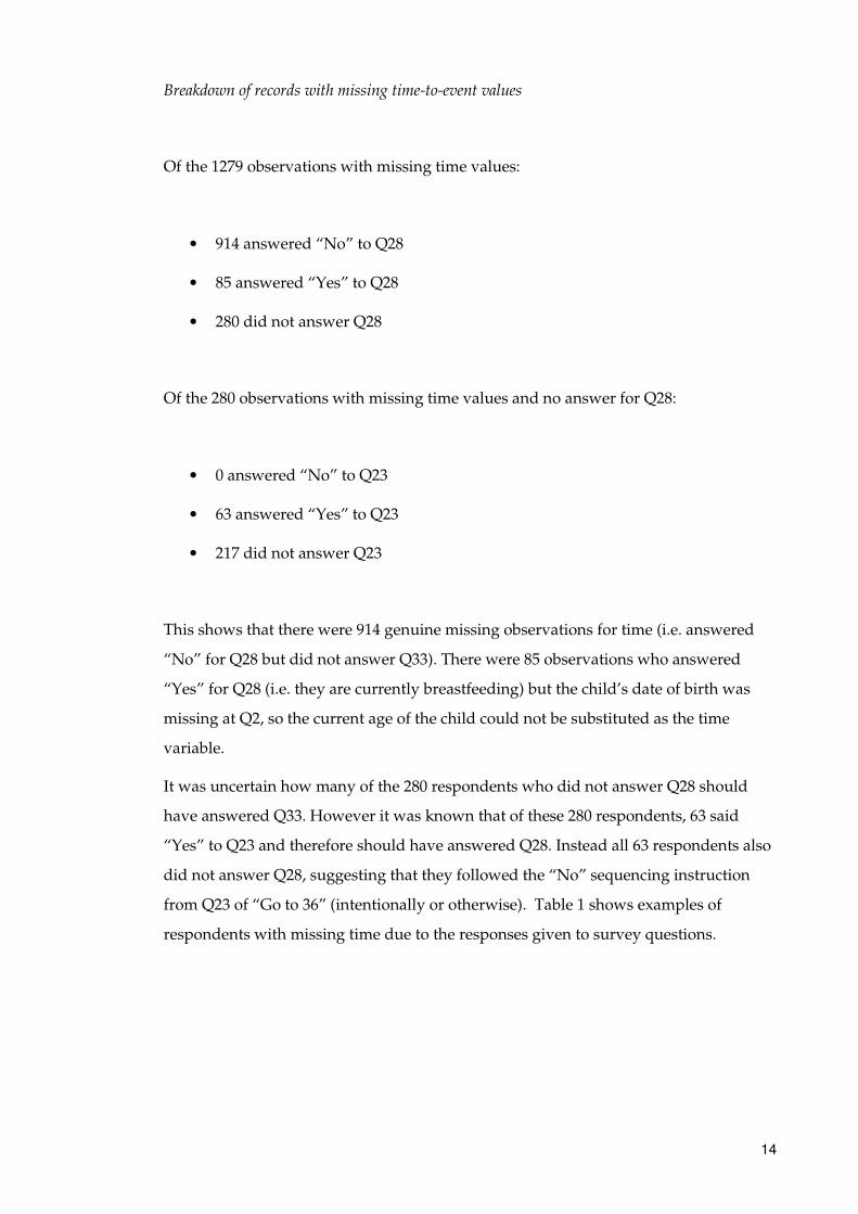
Breakdown of records with missing time-to-event values

Of the 1279 observations with missing time values:

• 914 answered “No” to Q28

• 85 answered “Yes” to Q28

• 280 did not answer Q28

Of the 280 observations with missing time values and no answer for Q28:

• 0 answered “No” to Q23

• 63 answered “Yes” to Q23

• 217 did not answer Q23

This shows that there were 914 genuine missing observations for time (i.e. answered

“No” for Q28 but did not answer Q33). There were 85 observations who answered

“Yes” for Q28 (i.e. they are currently breastfeeding) but the child’s date of birth was

missing at Q2, so the current age of the child could not be substituted as the time

variable.

It was uncertain how many of the 280 respondents who did not answer Q28 should

have answered Q33. However it was known that of these 280 respondents, 63 said

“Yes” to Q23 and therefore should have answered Q28. Instead all 63 respondents also

did not answer Q28, suggesting that they followed the “No” sequencing instruction

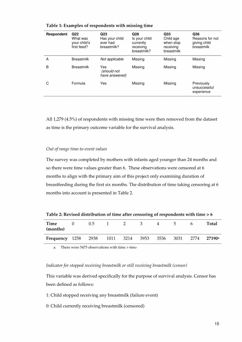
from Q23 of “Go to 36” (intentionally or otherwise). Table 1 shows examples of

respondents with missing time due to the responses given to survey questions.

15

Table 1: Examples of respondents with missing time

Respondent Q22 What was your child’s first feed?

Q23 Has your child ever had breastmilk?

Q28 Is your child currently receiving breastmilk?

Q33 Child age when stop receiving breastmilk

Q36 Reasons for not giving child breastmilk

A Breastmilk Not applicable Missing Missing Missing

B Breastmilk Yes (should not have answered)

Missing Missing Missing

C Formula Yes Missing Missing Previously unsuccessful experience

All 1,279 (4.5%) of respondents with missing time were then removed from the dataset

as time is the primary outcome variable for the survival analysis.

Out of range time-to-event values

The survey was completed by mothers with infants aged younger than 24 months and

so there were time values greater than 6. These observations were censored at 6

months to align with the primary aim of this project only examining duration of

breastfeeding during the first six months. The distribution of time taking censoring at 6

months into account is presented in Table 2.

Table 2: Revised distribution of time after censoring of respondents with time > 6

Time (months)

0 0.5 1 2 3 4 5 6 Total

Frequency 1258 2938 1011 3214 3953 3536 3031 2774 27190a

a. There were 5475 observations with time > 6mo

Indicator for stopped receiving breastmilk or still receiving breastmilk (censor)

This variable was derived specifically for the purpose of survival analysis. Censor has

been defined as follows:

1: Child stopped receiving any breastmilk (failure event)

0: Child currently receiving breastmilk (censored)

16

This was derived in Stata by using the following rules (see Appendix B for relevant

Stata code):

• Set censor to 0 if child currently receiving breastmilk.

• Set censor to 1 if either: child not currently receiving breastmilk, child never

had breastmilk, months (Q33b) not missing or less than one month (Q33a=0)

when stopped breastfeeding for Q33.

Mother’s age

Age was computed as the difference in years between the mother’s date of birth and

the date they completed the survey. Only respondents with calculated age between 15

and 50 years were kept in the dataset. Those aged less than 15 (179 records) or greater

than 50 (26 records) were removed from the dataset as they were the default values

chosen for average age at menarche and menopause respectively. Those with missing

age (64 records) were also removed. The variable was then categorised into four age

groups “15 to 24 years”, “25 to 29 years”, “30 to 34 years” and “35+ years” due to the

likely non-linear effect on survival.

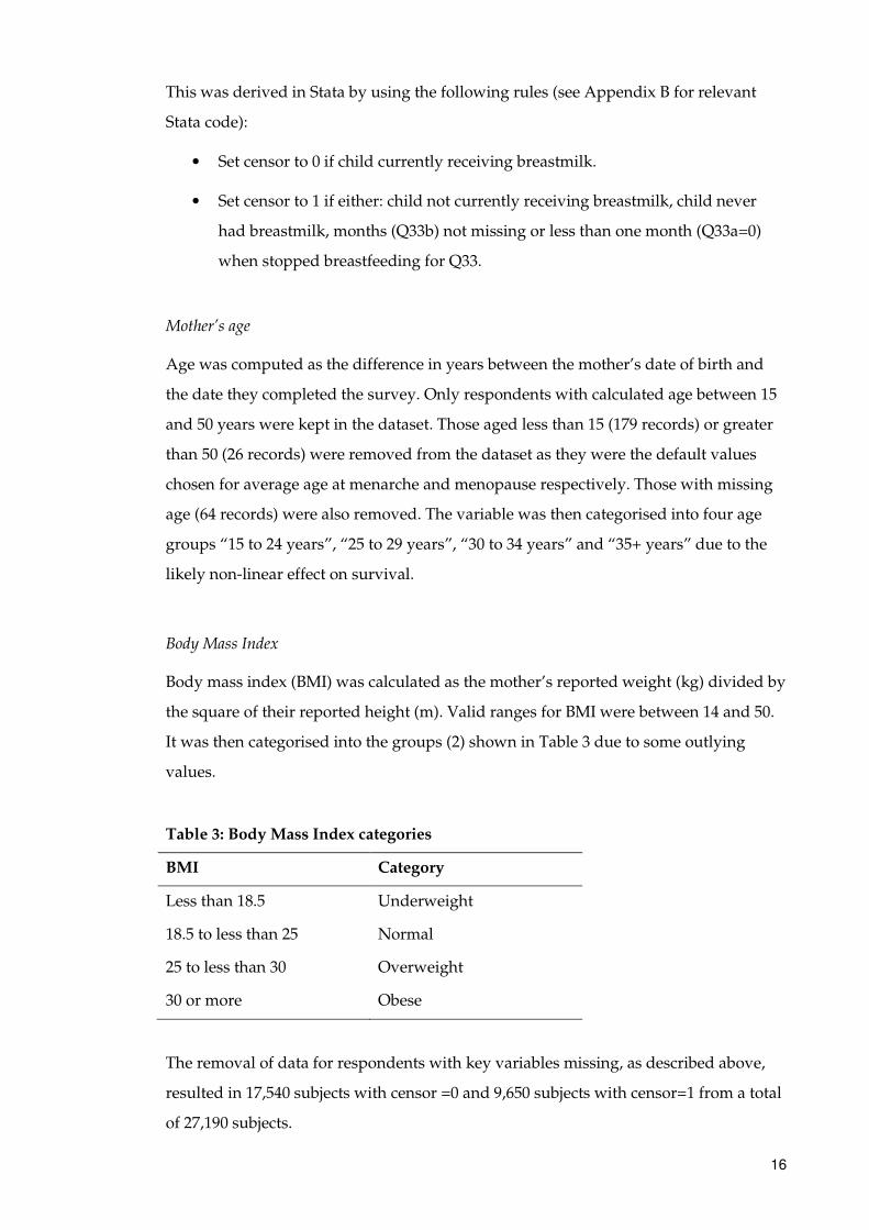
Body Mass Index

Body mass index (BMI) was calculated as the mother’s reported weight (kg) divided by

the square of their reported height (m). Valid ranges for BMI were between 14 and 50.

It was then categorised into the groups (2) shown in Table 3 due to some outlying

values.

Table 3: Body Mass Index categories

BMI Category

Less than 18.5 Underweight

18.5 to less than 25 Normal

25 to less than 30 Overweight

30 or more Obese

The removal of data for respondents with key variables missing, as described above,

resulted in 17,540 subjects with censor =0 and 9,650 subjects with censor=1 from a total

of 27,190 subjects.

17

Setting up data for survival analysis

Before survival analysis, data were set up in Stata using the stset command. The

variable in the failure option defines what a failure is. The default is for non-zero

values to represent failure event and zero to be censored values. In this case the failure

event for the censor variable is equal to 1.

If respondents with missing time variables were to be included then Stata would report

a “probable error” message, confirming that there is a potential problem with the time-

to-event data. This is what occurred when I initially set-up the data for survival

analysis and so removing the data for those respondents resulted in no more errors.

A summary of the data setup showed that, of the 27,190 total observations, 1,258

children were never breastfed and 8,392 children stopped receiving breastmilk

(experienced the event). There were 18,798 censored observations (i.e. the child was

breastfed for >6 months).

Restricting time to first six months

The K-M plots from the initial univariate analysis of breastfeeding up to 24 months

showed that mostly the effects of the predictors only held for the first six months. After

this the survival curves tended to cross. This subsequently led to problems validating

the proportional hazards assumption. To rectify this model violation it was decided

that the project aim would be restricted to predictors of breastfeeding to six months by

censoring observations at six months (still breastfeeding and ‘at risk’ of stopping). This

is also in accordance with previous literature and aligns with the World Health

Organisation (WHO) recommendations relating to the recommended duration of

breastfeeding before progressing to solid foods (2) (7) (8). This resulted in a further

5,475 observations being censored from the original analysis that included records with

duration of breastfeeding up to 24 months.

18

Statistical methods

Descriptive statistics

Characteristics of the data were examined to check the distribution of the covariates

and to ensure that none of the categories appeared too small, especially the number of

events (stopped breastfeeding), which is more important in survival analysis. The

23,181 children who were breastfed for at least one month were compared with those

who were breastfed for less than one month or never were (4,009 children) using a two-

sample t-test to determine whether the group means differed (Stata command: ttest).

For comparisons between categorical variables a chi-square test was used.

Univariate Analysis

Although the initial data set contained some continuous variables (Age, BMI), the

variables used in the univariate analysis were only categorical. This was mainly due to

the skewed nature of some of the continuous variables (e.g. BMI). The only continuous

variable used as a covariate in this analysis was therefore the survival time variable

itself (duration of breastfeeding).

Prior to undertaking any survival analysis the first step was to thoroughly examine the

association between the duration of breastfeeding and each of the covariates being

considered for inclusion in the model. As these are categorical covariates this analysis

comprised examining Kaplan-Meier (K-M) estimates of the group-specific survival

functions, hazard ratios and 95% confidence interval estimates, and performing log-

rank tests to compare survival for the covariate groups. Assessment of the global

significance for each variable was performed during univariate analysis to help decide

whether or not a variable should be included in the initial model building step.

Examples of K-M plots can be seen in Appendix A. The K-M plot showed age appeared

to have a non-linear effect on survival so it was decided that it should be categorised

rather than left as a continuous variable.

Multivariate Analysis

The method to determine covariates associated with the length of time a mother

provided breastmilk for their child was Cox multiple regression. The univariate

analysis of each independent variable using the Cox proportional hazards model (i.e.

19

stcox command in Stata) indicated which covariates would be entered in the initial

model. Covariates which were significant with P < 0.01 at univariate analysis were

included into the initial model as potential predictors of the duration of breastfeeding

for the final model, with the significance being tested by the likelihood ratio test

statistic.

Collinearity

Collinearity occurs when two or more covariates to be included in a model are closely

correlated, or nearly linearly dependent on each other. When this occurs it may make it

difficult to separate the effects of each covariate. A useful tool to diagnose these issues

is the variance-inflation factor (VIF) which is tested in Stata using the vif,

uncentered command. The square root of the VIF gives an approximation of how

much the standard error of the corresponding effect has increased due to collinearity

with the other covariates.

Variables deemed to be closely related in terms of what the variable was measuring

were assessed for collinearity. Variables suspected of collinearity were also checked to

see whether their standard errors and/or coefficient estimates changed noticeably

when they were added and removed during the model building process. If collinearity

was present between two variables that were closely related then only one of those

variables would be retained in the initial model. Previous findings relating to the

relevant subject matter were used to inform the decision between which of the two

collinear variables to include in the model.

Model development

There are a number of model building and variable selection methods that can be used

in survival analysis and most follow the same principles that were used for other types

of regression models presented in BCA units such as Linear Regression Models and

Categorical Data Analysis.

Building an appropriate multivariable model requires careful selection of relevant

variables. The method chosen for this process was the “purposeful selection” method

detailed in the prescribed Survival Analysis textbook by Hosmer, Lemeshow and May

(9). This method allows a lot of control in terms of how the variables are selected

20

compared to other more automated methods that use statistical algorithms for

selecting covariates such as the stepwise method.

The first step to building the model was to fit a model that contained all variables that

were significant in the univariate analysis, apart from those removed due to

collinearity. At this stage variables not significant could still be included if they were

deemed to be of clinical significance but none were included on this basis.

The resulting estimates from the initial fitted model and their associated P-values from

the Wald tests then determined what covariates could be removed from subsequent

refitting of the model. Non-significant covariates were removed one at a time as

reducing the size of the model too much at once could lead to the exclusion of what

perhaps could have been a significant covariate after refitting. For this reason a partial

likelihood ratio test was performed to ensure that the removed covariate was indeed

non-significant.

After fitting a model with a reduced set of covariates, the variable that was previously

excluded was checked to see if it was a confounder. These variables were judged to be

confounders if the estimated coefficients of the refitted model varied by more than

20%. If this was the case the variable was added back into the model. This process of

refitting the model after excluding a non-significant covariate was repeated until no

more covariates could be removed from the model.

All variables that were removed were then added back into the model one at a time to

check that these variables have remained non-significant and not an important

confounder. This step is not always considered a common step in variable selection

processes but sometimes variables that were initially non-significant could become

significant in the reduced model. Variables previously excluded due to collinearity

with other variables were also included again to confirm collinearity still existed in the

final model (e.g. checking the estimated coefficient intervals).

The last step in the variable selection process was to check if any interactions might be

required in the model. Any plausible interactions from the variables contained in the

reduced model from the previous step were checked by comparing the reduced model

with and without the interaction term using the likelihood ratio test.

21

Model adequacy

Test of proportional-hazards assumption

It is very important that the proportional hazards (PH) assumption is evaluated to

enable the correct interpretation and use of a fitted proportional hazards model. This

can be done using a method based on scaled Schoenfeld residuals (using stphtest in

Stata) which can be tested for each covariate (using the detail option) and for the

whole model. If the proportional hazards assumption is met, then a plot of the scaled

residuals over time should have slope of zero.

Overall goodness of fit

To test the overall goodness of fit of the final model, a plot of the cumulative hazard

function calculated from the Cox-Snell residuals should form a 45° line. This is

achieved by first fitting the final model and generating martingale residuals and then

generating the Cox-Snell residuals for the model. The data is then reset and the

variable containing the Cox-Snell residuals is specified as the time variable. From this

the Nelson-Aalen cumulative hazard function is generated and then graphed with the

Cox-Snell residuals to allow the comparison of the hazard function to the diagonal line.

See Appendix B for the Stata code used to generate the goodness-of-fit plot.

Results

Descriptive statistics

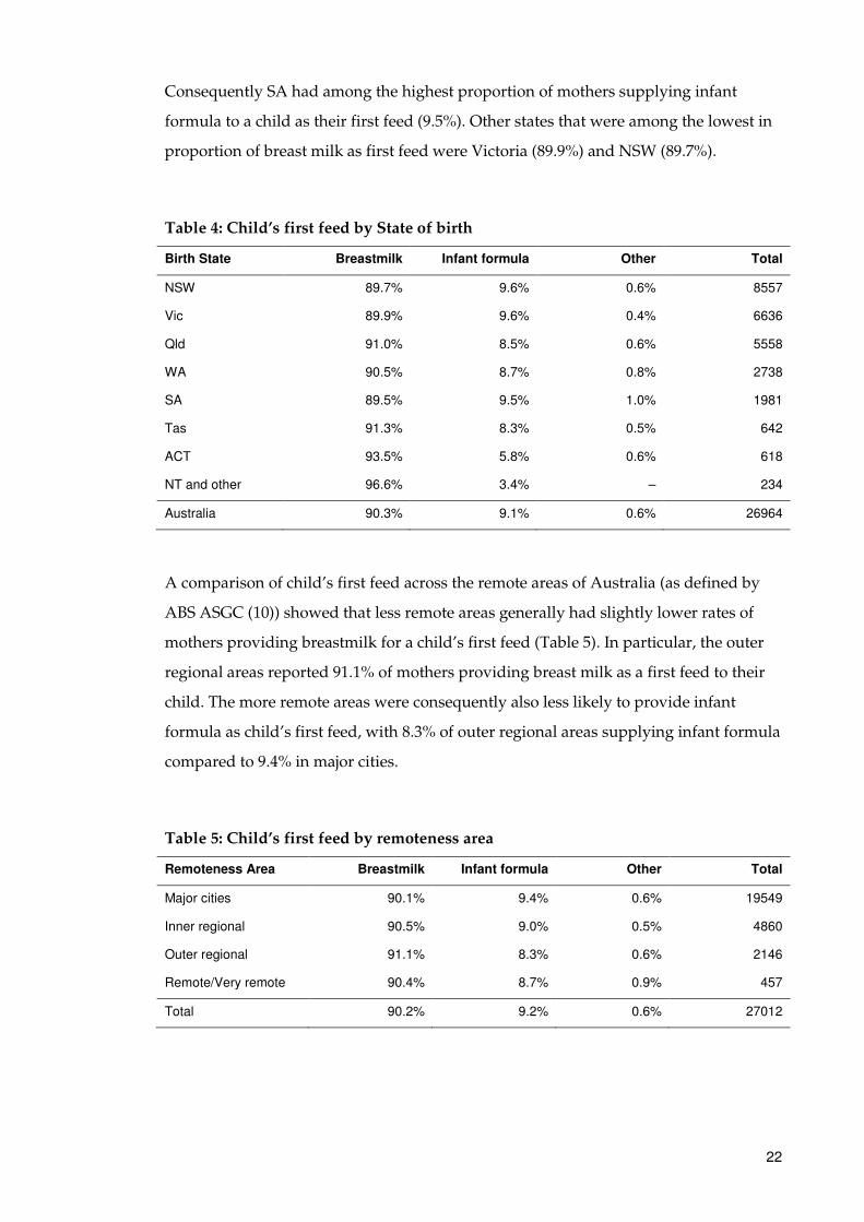
Table 4 compares the proportion of a child’s first type of feed across all states and

territories of Australia. The provision of breast milk as a new born child’s first feed was

most common in the NT (96.6%) compared to the national average of 90.3%. Other

states which had high rates of breastmilk as first feeds were ACT (93.5%), Tasmania

(91.3%) and Queensland (91.0%). The NT also had the lowest reported use of infant

formula as a first feed (3.4%) compared to national average of 9.1%. Together with the

ACT (5.8%) these territories had substantially lower proportions of infant formula as a

first feed than the rest of Australia. The state or territory which had the lowest

proportion of mothers who gave breast milk as their child’s first feed was SA (89.5%).

22

Consequently SA had among the highest proportion of mothers supplying infant

formula to a child as their first feed (9.5%). Other states that were among the lowest in

proportion of breast milk as first feed were Victoria (89.9%) and NSW (89.7%).

Table 4: Child’s first feed by State of birth

Birth State Breastmilk Infant formula Other Total

NSW 89.7% 9.6% 0.6% 8557

Vic 89.9% 9.6% 0.4% 6636

Qld 91.0% 8.5% 0.6% 5558

WA 90.5% 8.7% 0.8% 2738

SA 89.5% 9.5% 1.0% 1981

Tas 91.3% 8.3% 0.5% 642

ACT 93.5% 5.8% 0.6% 618

NT and other 96.6% 3.4% – 234

Australia 90.3% 9.1% 0.6% 26964

A comparison of child’s first feed across the remote areas of Australia (as defined by

ABS ASGC (10)) showed that less remote areas generally had slightly lower rates of

mothers providing breastmilk for a child’s first feed (Table 5). In particular, the outer

regional areas reported 91.1% of mothers providing breast milk as a first feed to their

child. The more remote areas were consequently also less likely to provide infant

formula as child’s first feed, with 8.3% of outer regional areas supplying infant formula

compared to 9.4% in major cities.

Table 5: Child’s first feed by remoteness area

Remoteness Area Breastmilk Infant formula Other Total

Major cities 90.1% 9.4% 0.6% 19549

Inner regional 90.5% 9.0% 0.5% 4860

Outer regional 91.1% 8.3% 0.6% 2146

Remote/Very remote 90.4% 8.7% 0.9% 457

Total 90.2% 9.2% 0.6% 27012

23

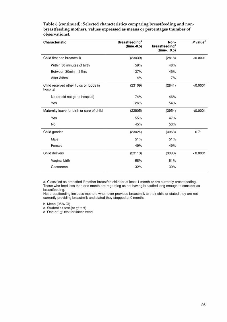
Comparison of breastfeeding and non-breastfeeding mothers

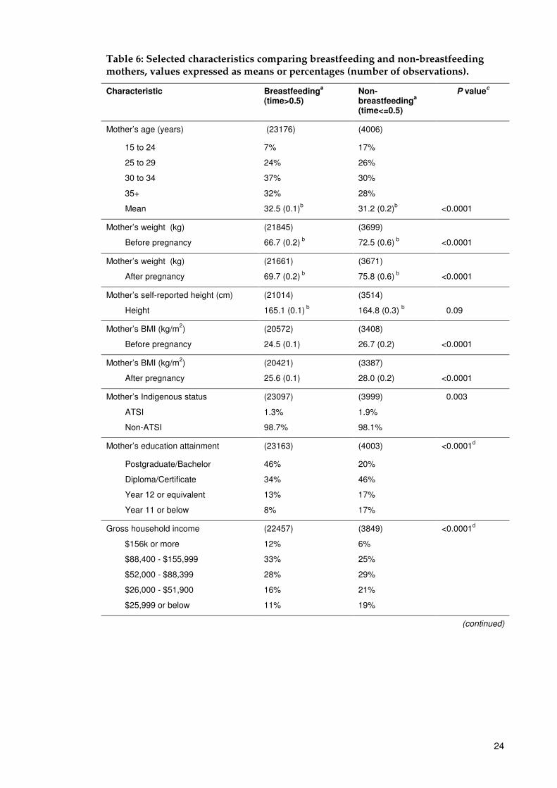
The mother and child characteristics presented in Table 6 have been categorised

according to the provision of breast milk to the child. Mothers who breastfed had a

lower pre-pregnancy and post-pregnancy weight than mothers who never provided

breastmilk to their child (mean difference of 5.8kg before pregnancy and 6.1kg after

pregnancy).

Mothers who did not breastfeed were younger than mothers who breastfed with only

7% of mothers who breastfed being aged 15 to 24 while 17% of mothers who did not

breastfeed were in this age group. In contrast, 37% of mothers who breastfed were

aged 30 to 34 and 32% were aged 35 and over.

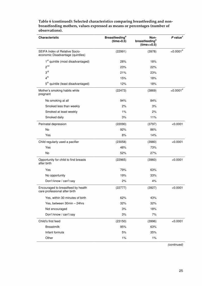
Among mothers who started breastfeeding, 79% gave the opportunity for their child to

find their breasts after birth compared to 63% for mothers who were not providing

breastmilk for their child. Among these same mothers, 59% provided breastmilk to

their child within 30 minutes of birth, 37% between 30 minutes and 24 hours and 4%

after 24 hours.

Pacifiers were used by 11,037 children (41%) during their first month of life with a

further 2,986 children (11%) first regularly using a pacifier after one month of age.

Mothers who breastfed for less than one month reported a higher proportion of regular

pacifier use (73%) than mothers who breastfed for more than one month (48%).

Other notable characteristics of the data showed that, compared to mothers who did

not breastfeed, mothers who breastfed had a lower pre and post birth weight, higher

proportion of postgraduate/bachelor degrees (46% vs. 20%), a generally higher gross

household income, lower proportion of those classified as disadvantaged socio-

economically, lower rates of perinatal depression, lower rates of smoking while

pregnant, lower use of pacifiers, provided more opportunities and encouragement for

their child to initiate breastfeeding, higher rates of maternity leave, and higher rates of

a natural birth method of child delivery.

24

Table 6: Selected characteristics comparing breastfeeding and non-breastfeeding mothers, values expressed as means or percentages (number of observations).

Characteristic Breastfeedinga

(time>0.5) Non-breastfeeding

a

(time<=0.5)

P valuec

Mother’s age (years) (23176) (4006)

15 to 24

25 to 29

30 to 34

35+

Mean

7%

24%

37%

32%

32.5 (0.1)b

17%

26%

30%

28%

31.2 (0.2)b

<0.0001

Mother’s weight (kg)

Before pregnancy

(21845)

66.7 (0.2) b

(3699)

72.5 (0.6) b

<0.0001

Mother’s weight (kg)

After pregnancy

(21661)

69.7 (0.2) b

(3671)

75.8 (0.6) b

<0.0001

Mother’s self-reported height (cm)

Height

(21014)

165.1 (0.1) b

(3514)

164.8 (0.3) b

0.09

Mother’s BMI (kg/m2)

Before pregnancy

(20572)

24.5 (0.1)

(3408)

26.7 (0.2)

<0.0001

Mother’s BMI (kg/m2)

After pregnancy

(20421)

25.6 (0.1)

(3387)

28.0 (0.2)

<0.0001

Mother’s Indigenous status

ATSI

Non-ATSI

(23097)

1.3%

98.7%

(3999)

1.9%

98.1%

0.003

Mother’s education attainment (23163) (4003) <0.0001d

Postgraduate/Bachelor

Diploma/Certificate

Year 12 or equivalent

Year 11 or below

46%

34%

13%

8%

20%

46%

17%

17%

Gross household income

$156k or more

$88,400 - $155,999

$52,000 - $88,399

$26,000 - $51,900

$25,999 or below

(22457)

12%

33%

28%

16%

11%

(3849)

6%

25%

29%

21%

19%

<0.0001d

(continued)

25

Table 6 (continued): Selected characteristics comparing breastfeeding and non-breastfeeding mothers, values expressed as means or percentages (number of observations).


(time>0.5) Non-

breastfeedinga

(time<=0.5)

P valuec

SEIFA Index of Relative Socio-economic Disadvantage (quintiles)

(22991) (3978) <0.0001d

1st quintile (most disadvantaged)

2nd

3rd

4th

5th

quintile (least disadvantaged)

28%

23%

21%

15%

12%

18%

22%

23%

18%

18%

Mother’s smoking habits while pregnant

(22473) (3869) <0.0001d

No smoking at all

Smoked less than weekly

Smoked at least weekly

Smoked daily

94%

2%

1%

3%

84%

3%

2%

11%

Perinatal depression

No

Yes

(22090)

92%

8%

(3797)

86%

14%

<0.0001

Child regularly used a pacifier

Yes

No

(23058)

48%

52%

(3980)

73%

27%

<0.0001

Opportunity for child to find breasts after birth

(22965) (3960) <0.0001

Yes

No opportunity

Don’t know / can’t say

79%

19%

2%

63%

33%

4%

Encouraged to breastfeed by health care professional after birth

(22777) (3927) <0.0001

Yes, within 30 minutes of birth

Yes, between 30min – 24hrs

Not encouraged


62%

32%

3%

3%

43%

32%

18%

7%

Child’s first feed

Breastmilk

Infant formula

Other

(23150)

95%

5%

1%

(3996)

63%

35%

1%

<0.0001

(continued)

26

Table 6 (continued): Selected characteristics comparing breastfeeding and non-breastfeeding mothers, values expressed as means or percentages (number of observations).


(time>0.5) Non-

breastfeedinga

(time<=0.5)

P valuec

Child first had breastmilk (23039) (2818) <0.0001

Within 30 minutes of birth

Between 30min – 24hrs

After 24hrs

59%

37%

4%

48%

45%

7%

Child received other fluids or foods in hospital

(23109) (2841) <0.0001

No (or did not go to hospital)

Yes

74%

26%

46%

54%

Maternity leave for birth or care of child (22905) (3954) <0.0001

Yes

No

55%

45%

47%

53%

Child gender (23024) (3963) 0.71

Male

Female

51%

49%

51%

49%

Child delivery (23113) (3998) <0.0001

Vaginal birth

Caesarean

68%

32%

61%

39%

a. Classified as breastfed if mother breastfed child for at least 1 month or are currently breastfeeding. Those who feed less than one month are regarding as not having breastfed long enough to consider as breastfeeding. Not breastfeeding includes mothers who never provided breastmilk to their child or stated they are not currently providing breastmilk and stated they stopped at 0 months.

b. Mean (95% CI) c. Student’s t-test (or χ2 test) d. One d.f. χ2 test for linear trend

27

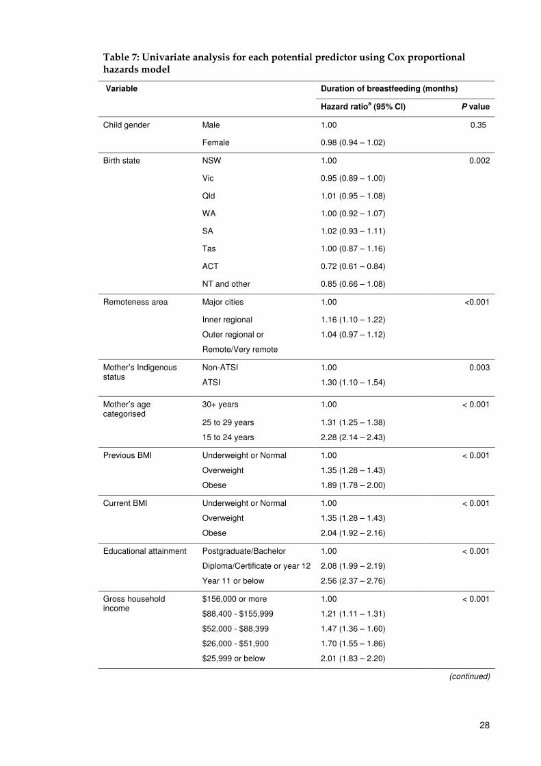
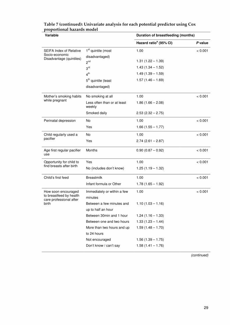
Univariate survival analysis

The results of the univariate survival analysis are presented in Table 7. All variables

except child gender (P=0.35) were significant at the 0.01 level so these variables make

up the initial starting model. Variables thus identified for inclusion in the initial model

as potential predictors of duration of breast feeding were: remoteness area, mothers

age, BMI before pregnancy, BMI after birth, educational attainment, gross household

income, SEIFA level, mothers smoking habits while pregnant, perinatal depression,

pacifier use, age child used pacifier, opportunity to find breasts after birth,

encouragement to breastfeed, child’s first feed, how soon had breastmilk, child

receiving other fluids in hospital, receiving breastmilk when first arrived home, and

child delivery method.

The estimates from the univariate analysis show that mothers with children born in

NSW had a 28% higher probability of stopping breastfeeding early than those born in

the ACT. This was one of the largest discrepancies between states with Queensland

and SA being the other states to have a higher probability of stopping early than NSW

(1% and 2% higher respectively). The median duration of breastfeeding for all states

was 4 months except for Tasmania which had a median duration of 3 months.

Total duration of breastfeeding

A number of variables were significantly associated with breastfeeding duration.

Among the factors that were associated with shorter duration of breastfeeding were:

low educational attainment by the mother (Year 11 or below: HR 2.56, 95% CI 2.37 –

2.76), low gross household income ($25,999 or below: HR 2.01, 95% CI 1.83 – 2.20), high

BMI of the mother after birth (obese: HR 2.04, 95% CI 1.92 – 2.16) and perinatal

depression (HR 1.66, 95% CI 1.55 – 1.77). In regard to factors relating to the initiation of

breastfeeding, having no opportunity for the child to find the mother’s breasts (HR

1.25, 95% CI 1.19 – 1.32), child’s first feed of infant formula (HR 1.78, 95% 1.65 – 1.92),

regularly using a pacifier (HR 2.74, 95% CI 2.61 – 2.87), the child being delivered by

caesarean (HR 1.27, 95% CI 1.21 – 1.33) and the mother being of Aboriginal or Torres

Strait Islander origin (HR 1.30, 95% CI 1.10 – 1.54) were also all associated with shorter

breastfeeding duration.

28

Table 7: Univariate analysis for each potential predictor using Cox proportional hazards model

Variable

Duration of breastfeeding (months)

Hazard ratioa (95% CI) P value

Child gender Male 1.00 0.35

Female 0.98 (0.94 – 1.02)

Birth state NSW 1.00 0.002

Vic 0.95 (0.89 – 1.00)

Qld 1.01 (0.95 – 1.08)

WA 1.00 (0.92 – 1.07)

SA 1.02 (0.93 – 1.11)

Tas 1.00 (0.87 – 1.16)

ACT 0.72 (0.61 – 0.84)

NT and other 0.85 (0.66 – 1.08)

Remoteness area Major cities 1.00 <0.001

Inner regional

Outer regional or

Remote/Very remote

1.16 (1.10 – 1.22)

1.04 (0.97 – 1.12)

Mother’s Indigenous status

Non-ATSI

ATSI

1.00

1.30 (1.10 – 1.54)

0.003

Mother’s age categorised

30+ years 1.00 < 0.001

25 to 29 years

15 to 24 years

1.31 (1.25 – 1.38)

2.28 (2.14 – 2.43)

Previous BMI Underweight or Normal

Overweight

Obese

1.00

1.35 (1.28 – 1.43)

1.89 (1.78 – 2.00)

< 0.001

Current BMI

Underweight or Normal

Overweight

Obese

1.00

1.35 (1.28 – 1.43)

2.04 (1.92 – 2.16)

< 0.001

Educational attainment


Diploma/Certificate or year 12

Year 11 or below

1.00

2.08 (1.99 – 2.19)

2.56 (2.37 – 2.76)

< 0.001


$156,000 or more

$88,400 - $155,999

$52,000 - $88,399

$26,000 - $51,900

$25,999 or below

1.00

1.21 (1.11 – 1.31)

1.47 (1.36 – 1.60)

1.70 (1.55 – 1.86)

2.01 (1.83 – 2.20)

< 0.001

(continued)

29

Table 7 (continued): Univariate analysis for each potential predictor using Cox proportional hazards model

Variable



SEIFA Index of Relative Socio-economic Disadvantage (quintiles)

1st quintile (most

disadvantaged)

2nd

3rd

4th

5th

quintile (least

disadvantaged)

1.00

1.31 (1.22 – 1.39)

1.43 (1.34 – 1.52)

1.49 (1.39 – 1.59)

1.57 (1.46 – 1.69)

< 0.001


No smoking at all

Less often than or at least weekly

Smoked daily

1.00

1.86 (1.66 – 2.08)

2.53 (2.32 – 2.75)

< 0.001


No

Yes

1.00

1.66 (1.55 – 1.77)

< 0.001


No

Yes

1.00

2.74 (2.61 – 2.87)

< 0.001

Age first regular pacifier use

Months 0.90 (0.87 – 0.92) < 0.001

Opportunity for child to find breasts after birth

Yes

No (includes don’t know)

1.00

1.25 (1.19 – 1.32)

< 0.001

Child’s first feed

Breastmilk

Infant formula or Other

1.00

1.78 (1.65 – 1.92)

< 0.001

How soon encouraged to breastfeed by health care professional after birth

Immediately or within a few

minutes

Between a few minutes and

up to half an hour

Between 30min and 1 hour

Between one and two hours

More than two hours and up

to 24 hours

Not encouraged


1.00

1.10 (1.03 – 1.16)

1.24 (1.16 – 1.33)

1.33 (1.23 – 1.44)

1.59 (1.48 – 1.70)

1.56 (1.39 – 1.75)

1.58 (1.41 – 1.76)

< 0.001

(continued)

30

Table 7 (continued): Univariate analysis for each potential predictor using Cox proportional hazards model

Variable



How soon after birth

child first had breastmilk

Immediately or within a few

minutes

Between a few minutes and

up to half an hour

Between 30min and 1 hour

Between one and two hours

More than two hours and up

to 24 hours

After 24 hours

1.00

1.12 (1.05 – 1.19)

1.30 (1.21 – 1.39)

1.34 (1.24 – 1.44)

1.63 (1.52 – 1.74)

2.07 (1.88 – 2.27)

< 0.001


No or Didn’t go to hospital

Yes

1.00

2.14 (2.05 – 2.24)

<0.001

Maternity leave for birth or care of child

Yes

No

1.00

1.09 (1.04 – 1.14)

<0.001

Child delivery method

Vaginal

Caesarean

1.00

1.27 (1.21 – 1.33)

<0.001

a. Hazard ratio for stopping breastfeeding

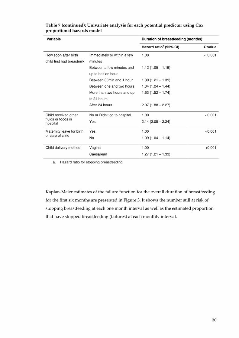
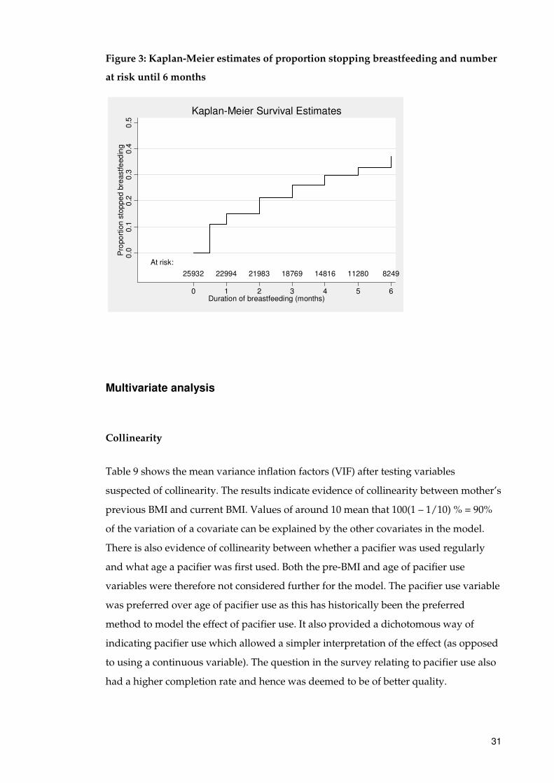
Kaplan-Meier estimates of the failure function for the overall duration of breastfeeding

for the first six months are presented in Figure 3. It shows the number still at risk of

stopping breastfeeding at each one month interval as well as the estimated proportion

that have stopped breastfeeding (failures) at each monthly interval.

31

Figure 3: Kaplan-Meier estimates of proportion stopping breastfeeding and number

at risk until 6 months

Multivariate analysis

Collinearity

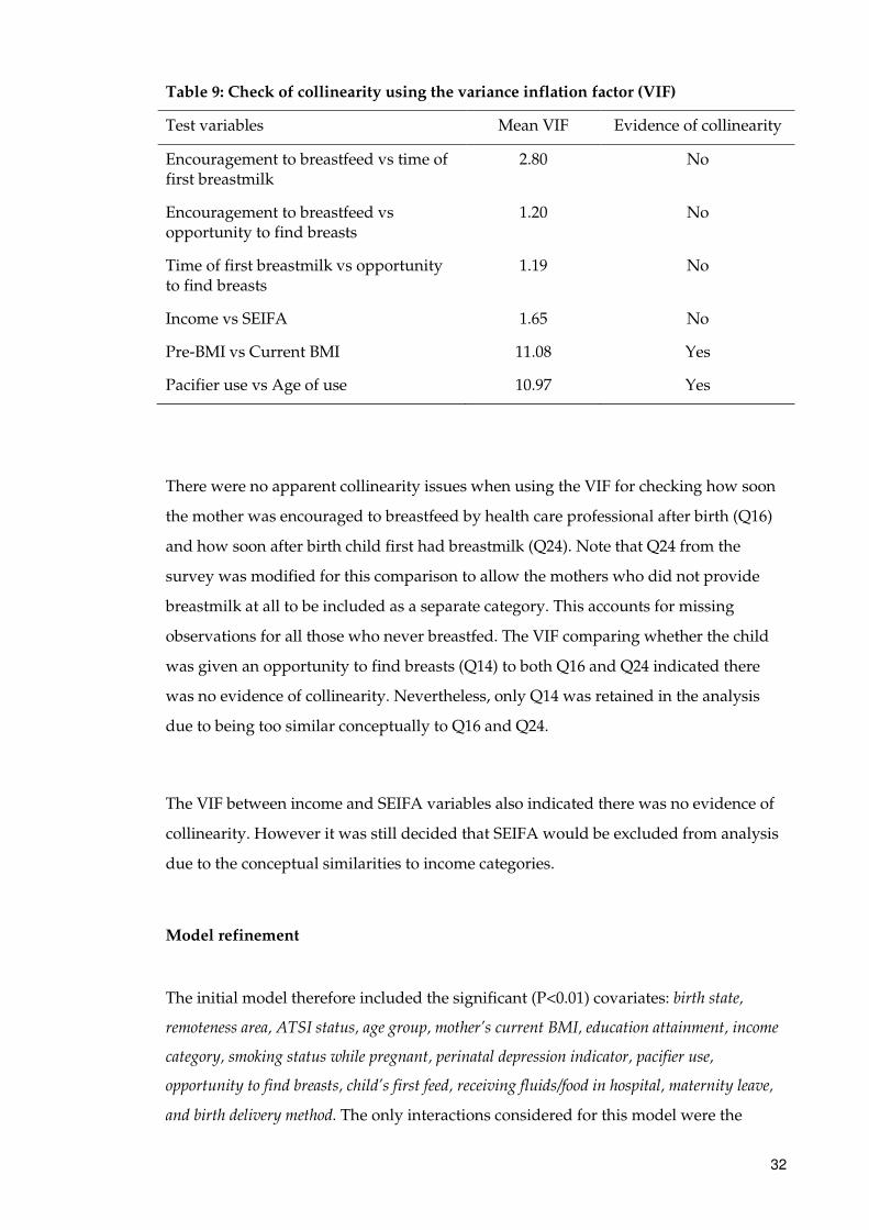
Table 9 shows the mean variance inflation factors (VIF) after testing variables

suspected of collinearity. The results indicate evidence of collinearity between mother’s

previous BMI and current BMI. Values of around 10 mean that 100(1 – 1/10) % = 90%

of the variation of a covariate can be explained by the other covariates in the model.

There is also evidence of collinearity between whether a pacifier was used regularly

and what age a pacifier was first used. Both the pre-BMI and age of pacifier use

variables were therefore not considered further for the model. The pacifier use variable

was preferred over age of pacifier use as this has historically been the preferred

method to model the effect of pacifier use. It also provided a dichotomous way of

indicating pacifier use which allowed a simpler interpretation of the effect (as opposed

to using a continuous variable). The question in the survey relating to pacifier use also

had a higher completion rate and hence was deemed to be of better quality.

At risk:

25932 22994 21983 18769 14816 11280 8249

0.0

0.1

0.2

0.3

0.4

0.5

Pro

po

rtio

n s

top

pe

d b

reastfe

ed

ing

0 1 2 3 4 5 6Duration of breastfeeding (months)

Kaplan-Meier Survival Estimates

32

Table 9: Check of collinearity using the variance inflation factor (VIF)

Test variables Mean VIF Evidence of collinearity

Encouragement to breastfeed vs time of first breastmilk

2.80 No

Encouragement to breastfeed vs opportunity to find breasts

1.20 No

Time of first breastmilk vs opportunity to find breasts

1.19 No

Income vs SEIFA 1.65 No

Pre-BMI vs Current BMI 11.08 Yes

Pacifier use vs Age of use 10.97 Yes

There were no apparent collinearity issues when using the VIF for checking how soon

the mother was encouraged to breastfeed by health care professional after birth (Q16)

and how soon after birth child first had breastmilk (Q24). Note that Q24 from the

survey was modified for this comparison to allow the mothers who did not provide

breastmilk at all to be included as a separate category. This accounts for missing

observations for all those who never breastfed. The VIF comparing whether the child

was given an opportunity to find breasts (Q14) to both Q16 and Q24 indicated there

was no evidence of collinearity. Nevertheless, only Q14 was retained in the analysis

due to being too similar conceptually to Q16 and Q24.

The VIF between income and SEIFA variables also indicated there was no evidence of

collinearity. However it was still decided that SEIFA would be excluded from analysis

due to the conceptual similarities to income categories.

Model refinement

The initial model therefore included the significant (P<0.01) covariates: birth state,

remoteness area, ATSI status, age group, mother’s current BMI, education attainment, income

category, smoking status while pregnant, perinatal depression indicator, pacifier use,

opportunity to find breasts, child’s first feed, receiving fluids/food in hospital, maternity leave,

and birth delivery method. The only interactions considered for this model were the

33

current BMI x age group and smoking while pregnant status x age group. However,

both interactions were non-significant at the 0.01 level and so were not included in the

reduced model.

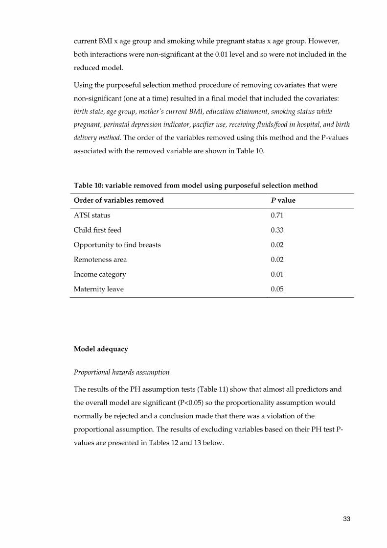
Using the purposeful selection method procedure of removing covariates that were

non-significant (one at a time) resulted in a final model that included the covariates:

birth state, age group, mother’s current BMI, education attainment, smoking status while

pregnant, perinatal depression indicator, pacifier use, receiving fluids/food in hospital, and birth

delivery method. The order of the variables removed using this method and the P-values

associated with the removed variable are shown in Table 10.

Table 10: variable removed from model using purposeful selection method

Order of variables removed P value

ATSI status 0.71

Child first feed 0.33

Opportunity to find breasts 0.02

Remoteness area 0.02

Income category 0.01

Maternity leave 0.05

Model adequacy

Proportional hazards assumption

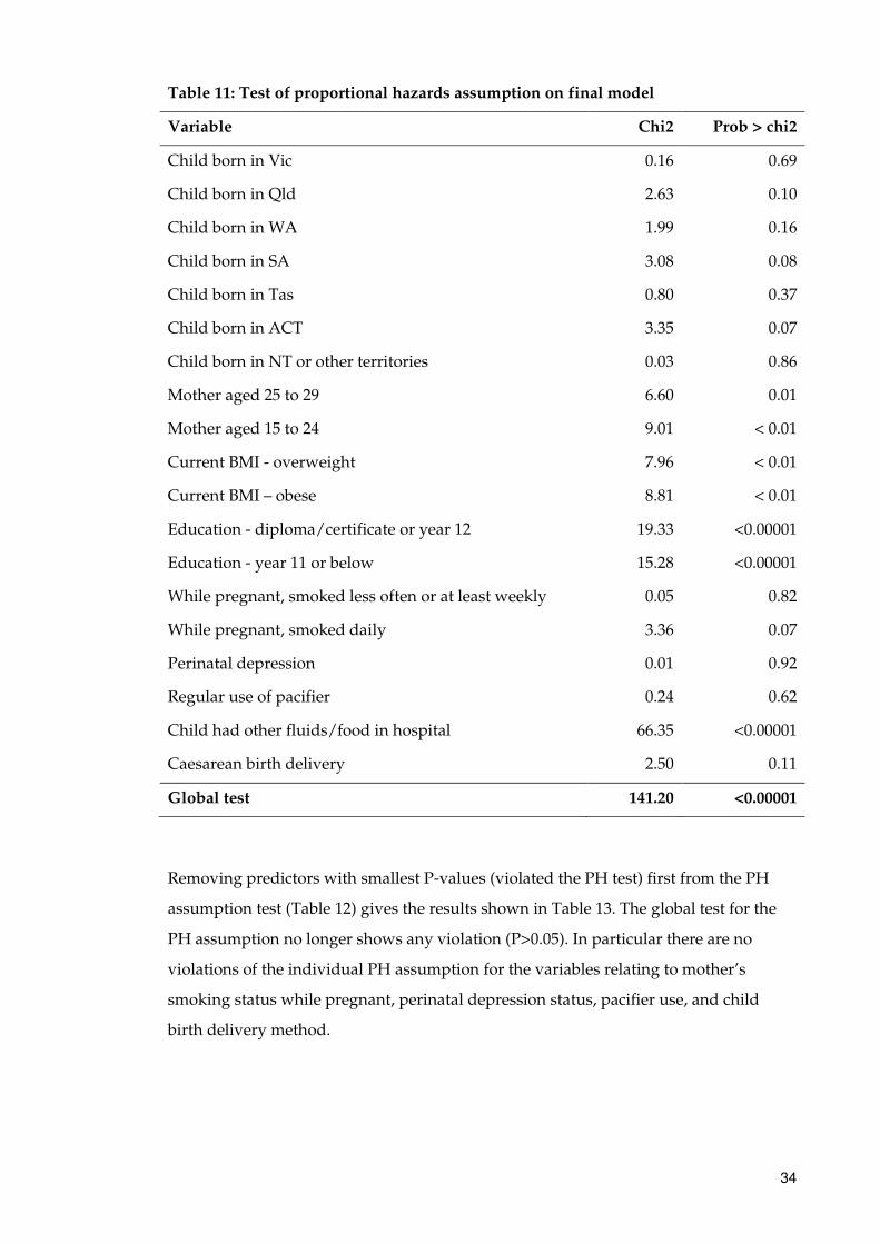
The results of the PH assumption tests (Table 11) show that almost all predictors and

the overall model are significant (P<0.05) so the proportionality assumption would

normally be rejected and a conclusion made that there was a violation of the

proportional assumption. The results of excluding variables based on their PH test P-

values are presented in Tables 12 and 13 below.

34

Table 11: Test of proportional hazards assumption on final model

Variable Chi2 Prob > chi2

Child born in Vic 0.16 0.69

Child born in Qld 2.63 0.10

Child born in WA 1.99 0.16

Child born in SA 3.08 0.08

Child born in Tas 0.80 0.37

Child born in ACT 3.35 0.07

Child born in NT or other territories 0.03 0.86

Mother aged 25 to 29 6.60 0.01

Mother aged 15 to 24 9.01 < 0.01

Current BMI - overweight 7.96 < 0.01

Current BMI – obese 8.81 < 0.01

Education - diploma/certificate or year 12 19.33 <0.00001

Education - year 11 or below 15.28 <0.00001

While pregnant, smoked less often or at least weekly 0.05 0.82

While pregnant, smoked daily 3.36 0.07

Perinatal depression 0.01 0.92

Regular use of pacifier 0.24 0.62

Child had other fluids/food in hospital 66.35 <0.00001

Caesarean birth delivery 2.50 0.11

Global test 141.20 <0.00001

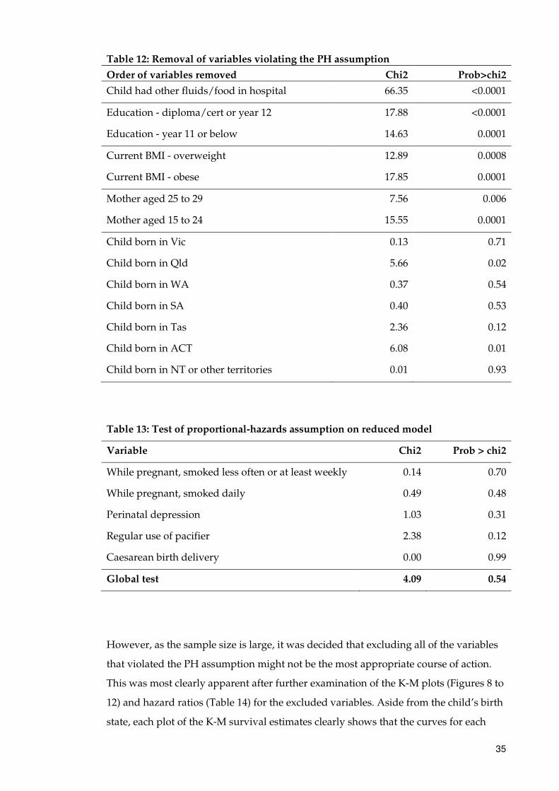
Removing predictors with smallest P-values (violated the PH test) first from the PH

assumption test (Table 12) gives the results shown in Table 13. The global test for the

PH assumption no longer shows any violation (P>0.05). In particular there are no

violations of the individual PH assumption for the variables relating to mother’s

smoking status while pregnant, perinatal depression status, pacifier use, and child

birth delivery method.

35

Table 12: Removal of variables violating the PH assumption

Order of variables removed Chi2 Prob>chi2

Child had other fluids/food in hospital 66.35 <0.0001

Education - diploma/cert or year 12 17.88 <0.0001

Education - year 11 or below 14.63 0.0001

Current BMI - overweight 12.89 0.0008

Current BMI - obese 17.85 0.0001

Mother aged 25 to 29 7.56 0.006

Mother aged 15 to 24 15.55 0.0001

Child born in Vic 0.13 0.71

Child born in Qld 5.66 0.02

Child born in WA 0.37 0.54

Child born in SA 0.40 0.53

Child born in Tas 2.36 0.12

Child born in ACT 6.08 0.01

Child born in NT or other territories 0.01 0.93

Table 13: Test of proportional-hazards assumption on reduced model

Variable Chi2 Prob > chi2

While pregnant, smoked less often or at least weekly 0.14 0.70

While pregnant, smoked daily 0.49 0.48

Perinatal depression 1.03 0.31

Regular use of pacifier 2.38 0.12

Caesarean birth delivery 0.00 0.99

Global test 4.09 0.54

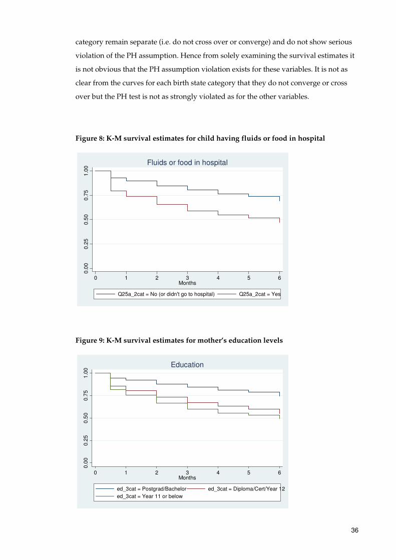
However, as the sample size is large, it was decided that excluding all of the variables

that violated the PH assumption might not be the most appropriate course of action.

This was most clearly apparent after further examination of the K-M plots (Figures 8 to

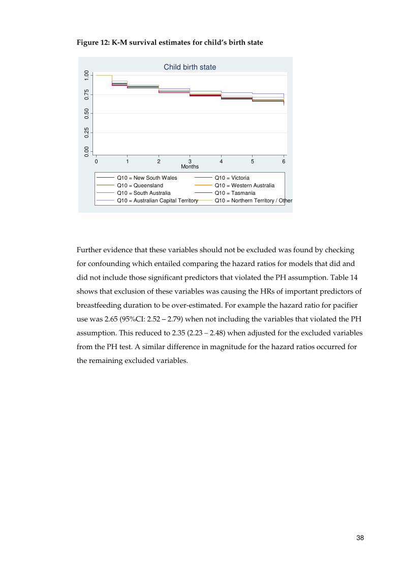
12) and hazard ratios (Table 14) for the excluded variables. Aside from the child’s birth

state, each plot of the K-M survival estimates clearly shows that the curves for each

36

category remain separate (i.e. do not cross over or converge) and do not show serious

violation of the PH assumption. Hence from solely examining the survival estimates it

is not obvious that the PH assumption violation exists for these variables. It is not as

clear from the curves for each birth state category that they do not converge or cross

over but the PH test is not as strongly violated as for the other variables.

Figure 8: K-M survival estimates for child having fluids or food in hospital

Figure 9: K-M survival estimates for mother’s education levels

0.0

00

.25

0.5

00

.75

1.0

0

0 1 2 3 4 5 6Months

Q25a_2cat = No (or didn't go to hospital) Q25a_2cat = Yes

Fluids or food in hospital

0.0

00

.25

0.5

00

.75

1.0

0

0 1 2 3 4 5 6Months

ed_3cat = Postgrad/Bachelor ed_3cat = Diploma/Cert/Year 12

ed_3cat = Year 11 or below

Education

37

Figure 10: K-M survival estimates for mother’s current BMI

Figure 11: K-M survival estimates for mother’s age category

0.0

00

.25

0.5

00

.75

1.0

0

0 1 2 3 4 5 6Months

bmicat_now2 = Underweight/normal bmicat_now2 = Overweight

bmicat_now2 = Obese

Current BMI0

.00

0.2

50

.50

0.7

51

.00

0 1 2 3 4 5 6Months

Q65_age2 = 30+ years Q65_age2 = 25-29 years

Q65_age2 = 15-24 years

Mother's age

38

Figure 12: K-M survival estimates for child’s birth state

Further evidence that these variables should not be excluded was found by checking

for confounding which entailed comparing the hazard ratios for models that did and

did not include those significant predictors that violated the PH assumption. Table 14

shows that exclusion of these variables was causing the HRs of important predictors of

breastfeeding duration to be over-estimated. For example the hazard ratio for pacifier

use was 2.65 (95%CI: 2.52 – 2.79) when not including the variables that violated the PH

assumption. This reduced to 2.35 (2.23 – 2.48) when adjusted for the excluded variables

from the PH test. A similar difference in magnitude for the hazard ratios occurred for

the remaining excluded variables.

0.0

00

.25

0.5

00

.75

1.0

0

0 1 2 3 4 5 6Months

Q10 = New South Wales Q10 = Victoria

Q10 = Queensland Q10 = Western Australia

Q10 = South Australia Q10 = Tasmania

Q10 = Australian Capital Territory Q10 = Northern Territory / Other

Child birth state

39

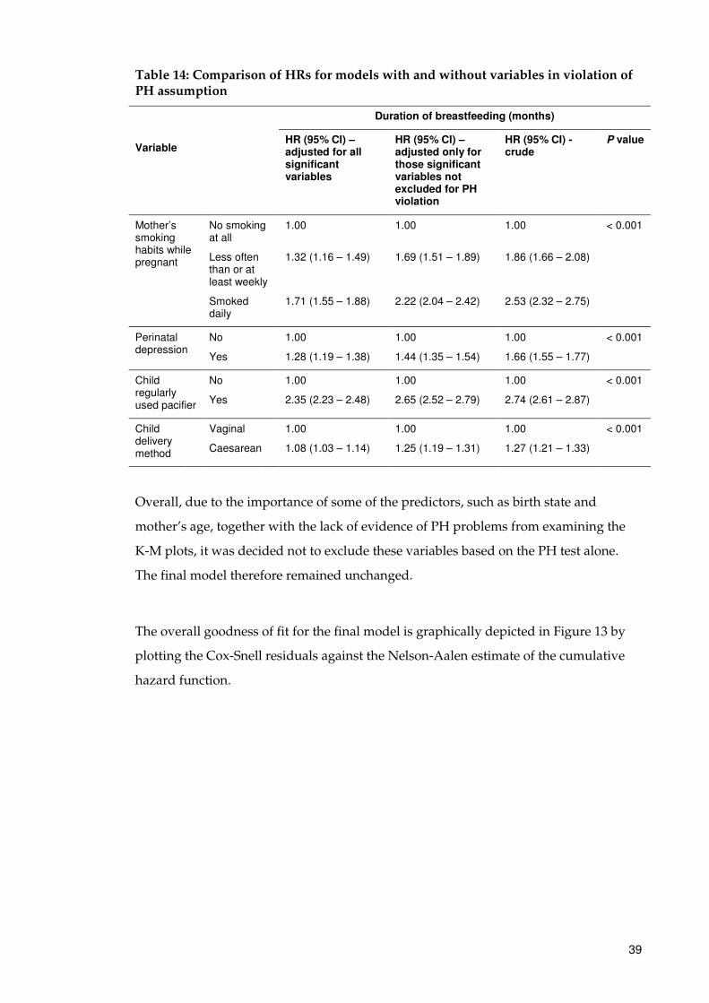
Table 14: Comparison of HRs for models with and without variables in violation of PH assumption

Variable


HR (95% CI) – adjusted for all significant variables

HR (95% CI) –adjusted only for those significant variables not excluded for PH violation

HR (95% CI) - crude

P value


No smoking at all


Smoked daily

1.00

1.32 (1.16 – 1.49)

1.71 (1.55 – 1.88)

1.00

1.69 (1.51 – 1.89)

2.22 (2.04 – 2.42)

1.00

1.86 (1.66 – 2.08)

2.53 (2.32 – 2.75)

< 0.001


No

Yes

1.00

1.28 (1.19 – 1.38)

1.00

1.44 (1.35 – 1.54)

1.00

1.66 (1.55 – 1.77)

< 0.001

Child regularly used pacifier

No

Yes

1.00

2.35 (2.23 – 2.48)

1.00

2.65 (2.52 – 2.79)

1.00

2.74 (2.61 – 2.87)

< 0.001


Vaginal

Caesarean

1.00

1.08 (1.03 – 1.14)

1.00

1.25 (1.19 – 1.31)

1.00

1.27 (1.21 – 1.33)

< 0.001

Overall, due to the importance of some of the predictors, such as birth state and

mother’s age, together with the lack of evidence of PH problems from examining the

K-M plots, it was decided not to exclude these variables based on the PH test alone.

The final model therefore remained unchanged.

The overall goodness of fit for the final model is graphically depicted in Figure 13 by

plotting the Cox-Snell residuals against the Nelson-Aalen estimate of the cumulative

hazard function.

40

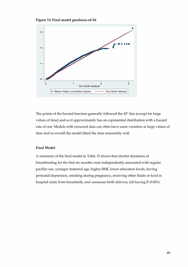
Figure 13: Final model goodness-of-fit

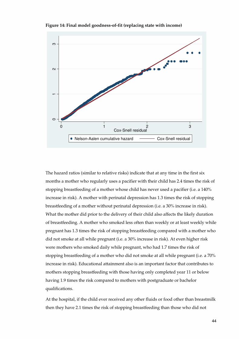
The points of the hazard function generally followed the 45° line (except for large

values of time) and so it approximately has an exponential distribution with a hazard

rate of one. Models with censored data can often have some variation at large values of

time and so overall the model fitted the data reasonably well.

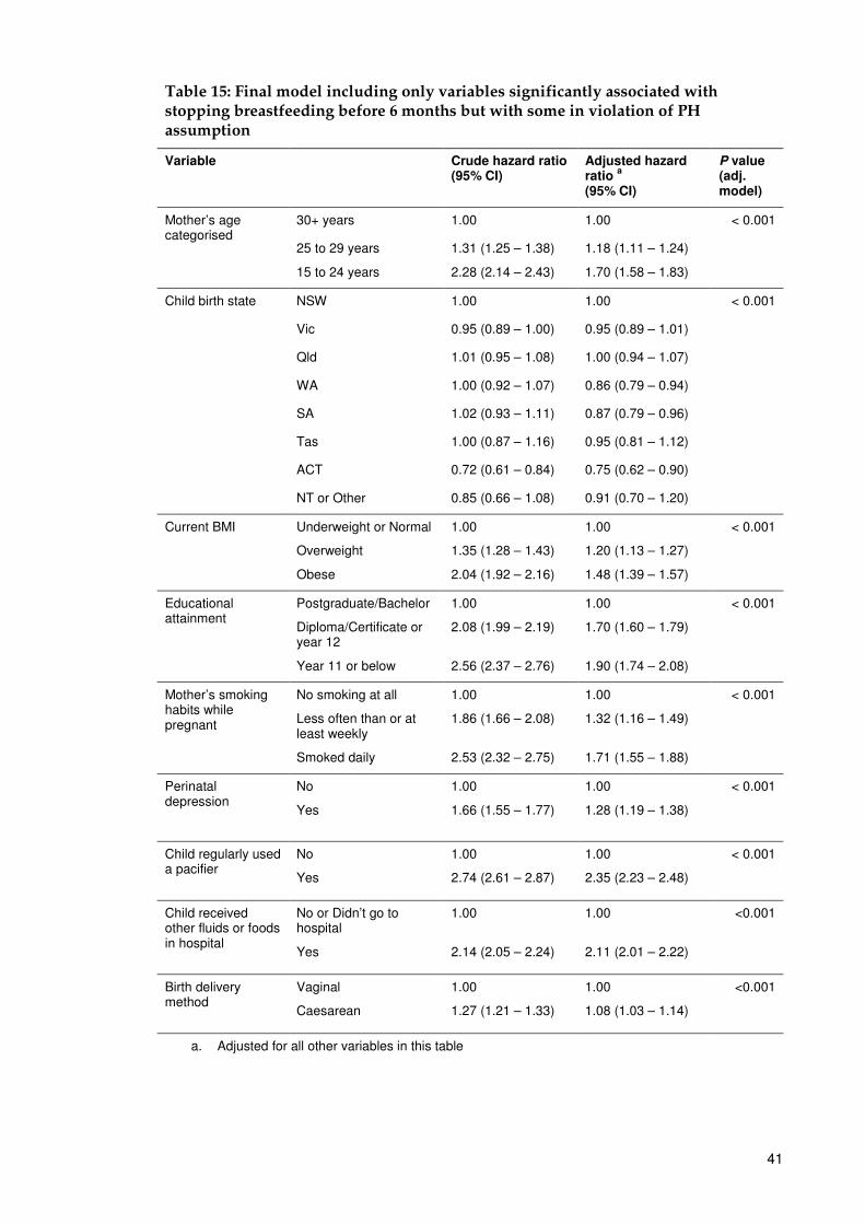
Final Model

A summary of the final model in Table 15 shows that shorter durations of

breastfeeding for the first six months were independently associated with regular

pacifier use, younger maternal age, higher BMI, lower education levels, having

perinatal depression, smoking during pregnancy, receiving other fluids or food in

hospital aside from breastmilk, and caesarean birth delivery (all having P<0.001).

01

23

0 1 2 3Cox-Snell residual

Nelson-Aalen cumulative hazard Cox-Snell residual

41

Table 15: Final model including only variables significantly associated with stopping breastfeeding before 6 months but with some in violation of PH assumption

Variable Crude hazard ratio (95% CI)

Adjusted hazard ratio

a

(95% CI)

P value (adj. model)


30+ years 1.00 1.00 < 0.001

25 to 29 years

15 to 24 years

1.31 (1.25 – 1.38)

2.28 (2.14 – 2.43)

1.18 (1.11 – 1.24)

1.70 (1.58 – 1.83)

Child birth state NSW 1.00 1.00 < 0.001

Vic 0.95 (0.89 – 1.00) 0.95 (0.89 – 1.01)

Qld 1.01 (0.95 – 1.08) 1.00 (0.94 – 1.07)

WA 1.00 (0.92 – 1.07) 0.86 (0.79 – 0.94)

SA 1.02 (0.93 – 1.11) 0.87 (0.79 – 0.96)

Tas 1.00 (0.87 – 1.16) 0.95 (0.81 – 1.12)

ACT 0.72 (0.61 – 0.84) 0.75 (0.62 – 0.90)

NT or Other 0.85 (0.66 – 1.08) 0.91 (0.70 – 1.20)

Current BMI


Overweight

Obese

1.00

1.35 (1.28 – 1.43)

2.04 (1.92 – 2.16)

1.00

1.20 (1.13 – 1.27)

1.48 (1.39 – 1.57)

< 0.001




Year 11 or below

1.00

2.08 (1.99 – 2.19)

2.56 (2.37 – 2.76)

1.00

1.70 (1.60 – 1.79)

1.90 (1.74 – 2.08)

< 0.001


No smoking at all


Smoked daily

1.00

1.86 (1.66 – 2.08)

2.53 (2.32 – 2.75)

1.00

1.32 (1.16 – 1.49)

1.71 (1.55 – 1.88)

< 0.001


No

Yes

1.00

1.66 (1.55 – 1.77)

1.00

1.28 (1.19 – 1.38)

< 0.001


No

Yes

1.00

2.74 (2.61 – 2.87)

1.00

2.35 (2.23 – 2.48)

< 0.001



Yes

1.00

2.14 (2.05 – 2.24)

1.00

2.11 (2.01 – 2.22)

<0.001

Birth delivery method

Vaginal

Caesarean

1.00

1.27 (1.21 – 1.33)

1.00

1.08 (1.03 – 1.14)

<0.001

a. Adjusted for all other variables in this table

42

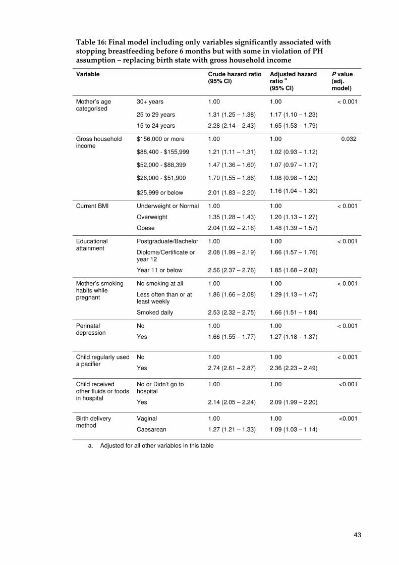
When income is cross-tabulated with birth state, states with the highest proportion of

mothers with a gross household income of over $88,400 were the ACT (68%) and NT

(52%). South Australia (35%) and Tasmania (34%) were among the lowest. ACT and

NT also had the lowest rates of mothers with a household income level below $26,000

(6% and 8% respectively) again compared with South Australia and Tasmania which,

together with New South Wales, had the equal highest rates in Australia (13%).

Because gross household income is more likely than state of residence to be causally

related to breastfeeding duration, a comparison of the final fitted model was made

with a model that replaced the state variable with the income variable (Table 16). It

showed that the model estimates with income and the overall goodness-of-fit varied

little, with the hazard ratios and standard errors slightly decreasing. Considering that

household income levels have also been associated with breastfeeding duration in

previous studies it was decided that income should replace state in the final model.

43

Table 16: Final model including only variables significantly associated with stopping breastfeeding before 6 months but with some in violation of PH assumption – replacing birth state with gross household income

Variable Crude hazard ratio (95% CI)

Adjusted hazard ratio

a

(95% CI)

P value (adj. model)


30+ years 1.00 1.00 < 0.001

25 to 29 years

15 to 24 years

1.31 (1.25 – 1.38)

2.28 (2.14 – 2.43)

1.17 (1.10 – 1.23)

1.65 (1.53 – 1.79)


$156,000 or more 1.00 1.00 0.032

$88,400 - $155,999 1.21 (1.11 – 1.31) 1.02 (0.93 – 1.12)

$52,000 - $88,399 1.47 (1.36 – 1.60) 1.07 (0.97 – 1.17)

$26,000 - $51,900 1.70 (1.55 – 1.86) 1.08 (0.98 – 1.20)

$25,999 or below 2.01 (1.83 – 2.20) 1.16 (1.04 – 1.30)

Current BMI


Overweight

Obese

1.00

1.35 (1.28 – 1.43)

2.04 (1.92 – 2.16)

1.00

1.20 (1.13 – 1.27)

1.48 (1.39 – 1.57)

< 0.001




Year 11 or below

1.00

2.08 (1.99 – 2.19)

2.56 (2.37 – 2.76)

1.00

1.66 (1.57 – 1.76)

1.85 (1.68 – 2.02)

< 0.001


No smoking at all


Smoked daily

1.00

1.86 (1.66 – 2.08)

2.53 (2.32 – 2.75)

1.00

1.29 (1.13 – 1.47)

1.66 (1.51 – 1.84)

< 0.001


No

Yes

1.00

1.66 (1.55 – 1.77)

1.00

1.27 (1.18 – 1.37)

< 0.001


No

Yes

1.00

2.74 (2.61 – 2.87)

1.00

2.36 (2.23 – 2.49)

< 0.001



Yes

1.00

2.14 (2.05 – 2.24)

1.00

2.09 (1.99 – 2.20)

<0.001

Birth delivery method

Vaginal

Caesarean

1.00

1.27 (1.21 – 1.33)

1.00

1.09 (1.03 – 1.14)

<0.001

a. Adjusted for all other variables in this table

44

Figure 14: Final model goodness-of-fit (replacing state with income)

The hazard ratios (similar to relative risks) indicate that at any time in the first six

months a mother who regularly uses a pacifier with their child has 2.4 times the risk of

stopping breastfeeding of a mother whose child has never used a pacifier (i.e. a 140%

increase in risk). A mother with perinatal depression has 1.3 times the risk of stopping

breastfeeding of a mother without perinatal depression (i.e. a 30% increase in risk).

What the mother did prior to the delivery of their child also affects the likely duration

of breastfeeding. A mother who smoked less often than weekly or at least weekly while

pregnant has 1.3 times the risk of stopping breastfeeding compared with a mother who

did not smoke at all while pregnant (i.e. a 30% increase in risk). At even higher risk

were mothers who smoked daily while pregnant, who had 1.7 times the risk of

stopping breastfeeding of a mother who did not smoke at all while pregnant (i.e. a 70%

increase in risk). Educational attainment also is an important factor that contributes to

mothers stopping breastfeeding with those having only completed year 11 or below

having 1.9 times the risk compared to mothers with postgraduate or bachelor

qualifications.

At the hospital, if the child ever received any other fluids or food other than breastmilk

then they have 2.1 times the risk of stopping breastfeeding than those who did not

01

23

0 1 2 3Cox-Snell residual

Nelson-Aalen cumulative hazard Cox-Snell residual

45

receive any (i.e. 110% increase in risk). The final factor that was found to have a strong

association with stopping breastfeeding was the type of birth delivery, mothers who

had a caesarean having 1.09 times the risk of stopping compared to mothers having a

vaginal delivery (i.e. a 9% increase in risk).

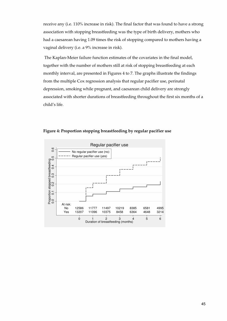
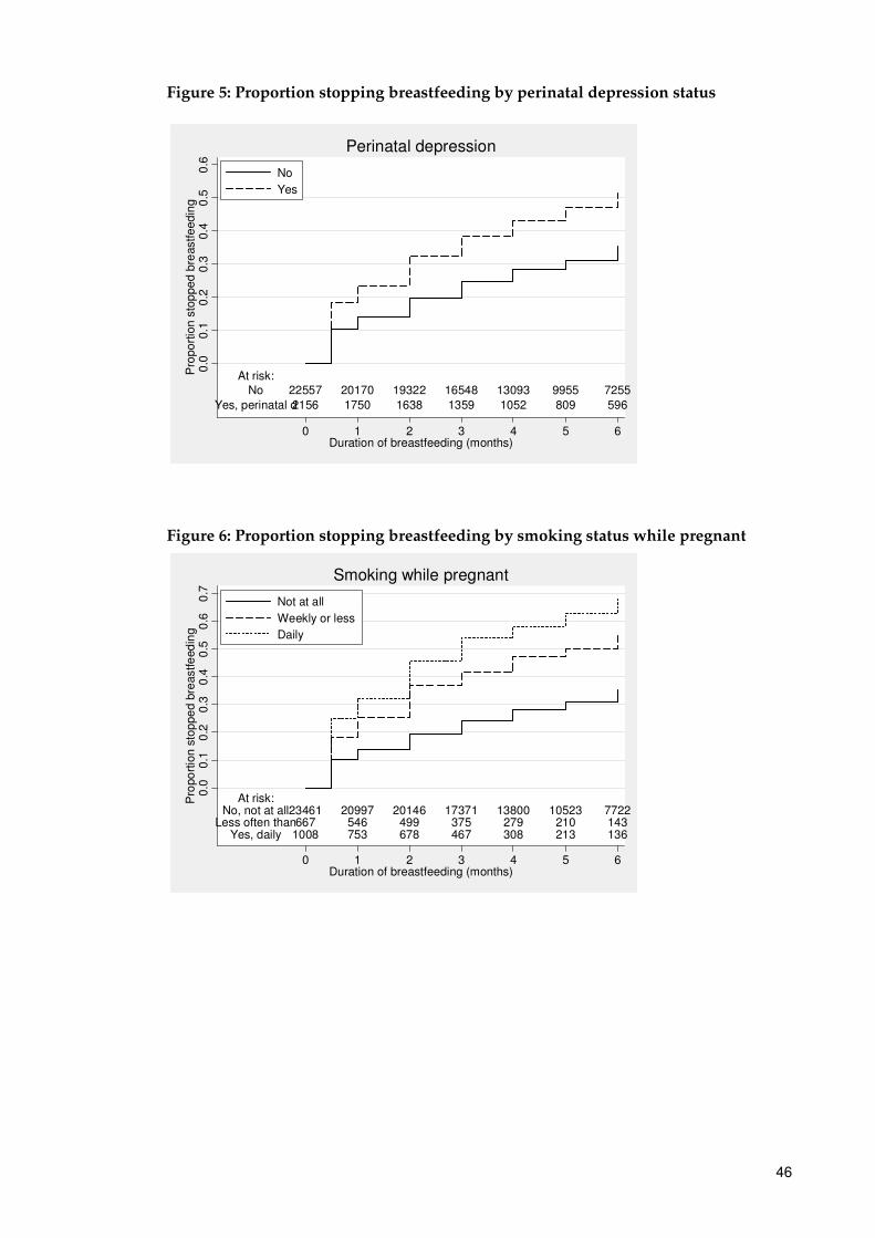
The Kaplan-Meier failure function estimates of the covariates in the final model,

together with the number of mothers still at risk of stopping breastfeeding at each

monthly interval, are presented in Figures 4 to 7. The graphs illustrate the findings

from the multiple Cox regression analysis that regular pacifier use, perinatal

depression, smoking while pregnant, and caesarean child delivery are strongly

associated with shorter durations of breastfeeding throughout the first six months of a

child’s life.

Figure 4: Proportion stopping breastfeeding by regular pacifier use

At risk:No 12586 11777 11497 10219 8385 6581 4995

Yes 13207 11096 10375 8458 6364 4648 3214

0.0

0.1

0.2

0.3

0.4

0.5

0.6

Pro

po

rtio

n s

top

pe

d b

reastfe

ed

ing


No regular pacifier use (no)

Regular pacifier use (yes)

Regular pacifier use

46

Figure 5: Proportion stopping breastfeeding by perinatal depression status

Figure 6: Proportion stopping breastfeeding by smoking status while pregnant

At risk:No 22557 20170 19322 16548 13093 9955 7255

Yes, perinatal d2156 1750 1638 1359 1052 809 596

0.0

0.1

0.2

0.3

0.4

0.5

0.6

Pro

po

rtio

n s

top

pe

d b

reastfe

ed

ing


No

Yes


At risk:No, not at all23461 20997 20146 17371 13800 10523 7722

Less often than667 546 499 375 279 210 143Yes, daily 1008 753 678 467 308 213 136

0.0

0.1

0.2

0.3

0.4

0.5

0.6

0.7

Pro

po

rtio

n s

top

pe

d b

reastfe

ed

ing


Not at all

Weekly or less

Daily

Smoking while pregnant

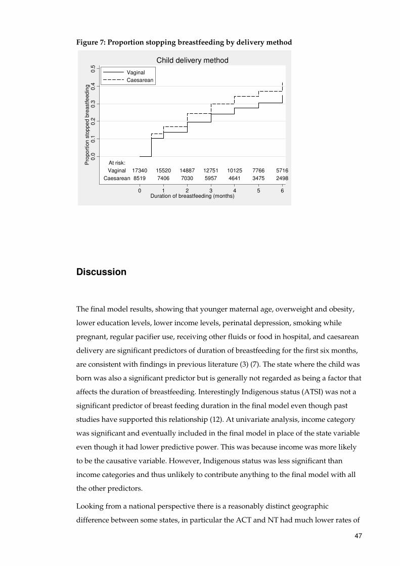
47

Figure 7: Proportion stopping breastfeeding by delivery method

Discussion

The final model results, showing that younger maternal age, overweight and obesity,

lower education levels, lower income levels, perinatal depression, smoking while

pregnant, regular pacifier use, receiving other fluids or food in hospital, and caesarean

delivery are significant predictors of duration of breastfeeding for the first six months,

are consistent with findings in previous literature (3) (7). The state where the child was

born was also a significant predictor but is generally not regarded as being a factor that

affects the duration of breastfeeding. Interestingly Indigenous status (ATSI) was not a

significant predictor of breast feeding duration in the final model even though past

studies have supported this relationship (12). At univariate analysis, income category

was significant and eventually included in the final model in place of the state variable

even though it had lower predictive power. This was because income was more likely

to be the causative variable. However, Indigenous status was less significant than

income categories and thus unlikely to contribute anything to the final model with all

the other predictors.

Looking from a national perspective there is a reasonably distinct geographic

difference between some states, in particular the ACT and NT had much lower rates of

At risk:

Vaginal 17340 15520 14887 12751 10125 7766 5716

Caesarean 8519 7406 7030 5957 4641 3475 2498

0.0

0.1

0.2

0.3

0.4

0.5

Pro

po

rtio

n s

top

pe

d b

reastfe

ed

ing


Vaginal

Caesarean


48

stopping breastfeeding in the first six months than the rest of Australia. One

explanation (at least for the ACT) for this result could be due to the high proportion of

public servants in the ACT compared to the rest of Australia, where over one-third of

Australian Public Service are located (13). The public service provides flexible working

hours and generous maternity leave benefits that are not always available in the

private sector (14) which would allow mothers to spend more time with their child and

subsequently allow more opportunities to establish regular breastfeeding.

Also highlighting this geographical difference is the effect a mother’s income has on

breastfeeding duration. Income alone is strongly associated with breastfeeding

duration where mothers on a higher income are more likely to breastfed longer than

those on a lower income. In particular, the rate of breastfeeding becomes progressively

lower for each drop in income category. When income was cross-tabulated with birth

state, we saw that states which had the highest of proportion mothers with a gross

household income of over $88,400 were the ACT and NT, which also had the lowest

rates of stopping breastfeeding early. These findings also support the notion of the

higher proportion of public service positions in the ACT and hence an environment

more conducive to the encouragement, and opportunity, to establish early and

sustained breastfeeding practices.

Mother’s BMI was strongly associated with breastfeeding duration and there was a

clear pattern which suggested those who were overweight (and especially obese) were

more likely to stop breastfeeding earlier than those who were underweight or at

normal weight. This might be interpreted that biological factors are preventing

mothers from breastfeeding longer due to excess weight (15), possibly related to

decreased levels of prolactin (16). There could also be a false perception that

breastfeeding has caused weight gain. This may cause these mothers to stop

breastfeeding in an attempt to limit weight gain they have attributed to breastfeeding.

One of the main issues encountered in the application of survival analysis to the

original subset of survey data were resulting models that did not fit the data. The first

subset of data comprised mothers who breast fed up until 24 months, but this resulted

in models that clearly violated the proportional hazard assumption which is vital when

attempting to interpret Cox regression models. Revising the scope of data to include

only mothers who breastfed up to 12 months was done in an attempt to rectify this but

again the assumption was violated. Eventually a decision was made to censor

49

observations for mothers who breastfed over six months which resulted in the

proportional hazards assumption being better satisfied.

It was clear from the diagnostic tests of the independent variables that many K-M plots

had lines that were separated to a certain time upon which the lines would converge

(usually around the 6 to 9 month mark). After careful consideration it was determined

that the most likely cause for this was twofold. First, a large proportion of mothers who

take maternity leave typically are on leave for up to six months. This would coincide

with the time of convergence of the K-M plots. Second, the six-month target for

breastfeeding duration is often emphasised by health professionals and health studies

(7) (8) (17) (18), including being recommended by WHO (2). This would be the case

irrespective of a woman’s parental leave issues. Again, this might explain the

convergence in the K-M plots at 6 months.

Mothers with lower levels of completed educational qualifications were more likely to

stop breastfeeding earlier than mothers who had completed a postgraduate

qualification or bachelor degree. Education levels also align with the income levels (i.e.

socio-economic status) which are supported by many studies (11) (19) (20) that have

found socially disadvantaged mothers begin breast feeding less often and also

breastfeed for a shorter duration. This would suggest that less-educated women should

be among the target groups for the promotion of breastfeeding and raising awareness

levels of the benefits both in financial and health terms.

An area of the survey that would have been worth investigating was alcohol use. It is

widely accepted (21) that alcohol should not be consumed during pregnancy due to the

risk it poses to the unborn child’s natural development, not to mention the risk to the

mother herself. As smoking status was collected it seems surprising that alcohol

consumption was not, especially since smoking was determined to have a strong

association with shorter duration of breastfeeding. Alcohol consumption could

conceivably have a similar affect on breastfeeding duration as smoking does so it

would be worthwhile collecting data on this area for the next national survey.

50

Conclusion

Overall, the factors that were determined to be associated with the duration of

breastfeeding for the child’s first six months are consistent with previous literature (3)

(7). Pacifier use in particular has been known for some time to be a leading factor in

reducing the duration of breastfeeding. Other factors such as smoking status while

pregnant and perinatal depression status have been also been linked to duration of

breastfeeding in previous studies but has not been as widely reported as a major factor

as pacifier use. There is also research that fewer women breastfeed their child after

having a caesarean (22) which also aligns with the analysis results. Typically the

reasoning for this association is the inability of women to breastfeed conveniently in

the period just after the delivery of their child.

A national perspective of the survey results showed that ACT was among the leading

states in the percentage of children who provided breastmilk for a child’s first feed. It

also had the highest rates of breastfeeding duration. The NT was also surprisingly high

with no clear explanation for this, although the data sample for NT is the smallest of

the eight states and territories. Nationally it is still clear that breastfeeding duration

could be substantially improved. Australia in comparison to the rest of the world ranks

around the middle in breastfeeding duration rates (23) and the results from this project

help to identify the groups of mothers that should be targeted for improved support

and education to enable the more widespread practice of breastfeeding in Australia. A

recent study (8) on first-time mothers in Sydney showed that a substantial number of

mothers were not aware of the breastfeeding practices recommended by WHO. In

particular, mothers with low levels of education were less likely to be aware of the

recommendations than those with tertiary education. This again aligns with the

findings in this project in relation to the association between mother’s education levels

and breastfeeding duration and is a further indication of the need for increasing the

promotion of breastfeeding in Australia.

51

Bibliography

1. Heller, G, Graham, P and Beath, K. Survival Analysis: Unit of Study Notes. Sydney : Department of Statistics, Macquarie University, 2011.

2. World Health Organization. Global strategy for infant and young child feeding. WHO. [Online] [Cited: 26 July 2011.] http://www.who.int/child_adolescent_health/topics/prevention_care/child/nutrition/global/en/.

3. Australian Institute of Health and Welfare. A picture of Australia’s children. Canberra : AIHW, 2009. Cat. no. PHE 112.

4. National Health and Medical Research Council. Dietary Guidelines for Children and Adolescents in Australia incorporating the Infant Feeding Guidelines for Health Workers. NHMRC. [Online] 2003. [Cited: 2 August 2011.] www.nhmrc.gov.au/PUBLICATIONS/synopses/_files/n34.pdf.

5. Baxter, J. Breastfeeding, employment and leave: An analysis of mothers in Growing Up in Australia. Australian Institute of Family Studies. 2008.

6. Australian Institute of Health and Welfare. Australian National Infant Feeding Survey 2010. [Questionairre] 2010.

7. Australian Government Department of Health and Ageing. The Australian National Breastfeeding Strategy 2010-2015. Canberra : s.n., 2009.

8. Wen, L M; Baur, L A; Rissel, C; Alperstein, G; Simpson, JM. Intention to breastfeed and awareness of health recommendations:findings from first-time mothers in southwest Sydney, Australia. International Breastfeeding Journal. 2009, Vol. 4, 9.

9. Hosmer, DW, Stanley, L and May, S. Applied Survival Analysis: regression modelling of time-to-event data, second edition. New Jersey : John Wiley & Sons, 2008.

10. Australian Bureau of Statistics. 1216.0 - Australian Standard Geographical Classification (ASGC) . ABS. [Online] July 2006. http://www.abs.gov.au/ausstats/[email protected]/Latestproducts/1AE106C101420508CA2571A900170741?opendocument.

11. Amir, L and Donath, S. Socioeconomic status and rates of breastfeeding in Australia: evidence from three recent national health surveys. Medical Journal of Australia. [Online] 2008. http://www.mja.com.au/public/issues/189_05_010908/ami11480_fm.html.

12. Australian Health Ministers’ Advisory Council. Aboriginal and Torres Strait Islander Health Performance Framework Report. Canberra : AHMAC, 2008.

13. Australian Public Service Commission. State of the Service report 2008-09. APSC. [Online] June 2009. [Cited: 22 August 2011.] http://www.apsc.gov.au/stateoftheservice/0809/measuringtheworkforce.html.

14. Australian Bureau of Statistics. 4913.0 - Pregnancy and Employment Transitions, Australia . ABS. [Online] November 2005. http://www.abs.gov.au/AUSSTATS/[email protected]/Lookup/4913.0Main+Features1Nov%202005?OpenDocument.

52

15. Rutishauser, IH and Carlin, JB. Body mass index and duration of breast feeding: a survival analysis during the first six months of life. Journal of Epidemiology and Community Health. 1992, 46, pp. 559-565.

16. Oddy, WH et al. The association of maternal overweight and obesity with breastfeeding duration. The Journal of Pediatrics. 2006, Vol. 149, 2, pp. 185-191.

17. Australian Institute of Health and Welfare. National breastfeeding indicators: workshop report. Canberra : AIHW, 2011. Cat. no. PHE 146.

18. Australian Government. Australian Government Response to The Best Start: Report on the inquiry into the health benefits of breastfeeding. Parliament of Australia. [Online] December 2008. [Cited: 2 August 2011.] www.aph.gov.au/house/committee/haa/breastfeeding/bfgovresp.pdf.

19. Australian Bureau of Statistics. Australian social trends 2007. Canberra : s.n.

20. van Rossem, L et al. Are Starting and Continuing Breastfeeding Related to Educational Background? The Generation R Study. Pediatrics. June 2009, Vol. 123, 6, pp. 1017-1027.

21. National Health and Medical Research Council. Australian Guidelines to Reduce Health Risks from Drinking Alcohol. NHMRC. [Online] 2009. [Cited: 22 August 2011.] http://www.nhmrc.gov.au/_files_nhmrc/publications/attachments/ds10-alcohol.pdf.

22. Zanardo V, et al. Elective cesarean delivery: does it have a negative effect on breastfeeding? PubMed. 2010, Vol. 37, 4.

23. Organisation for Economic Co-operation and Development. CO1.5: Breastfeeding rates. OECD. [Online] 2009. [Cited: 22 August 2011.] http://www.oecd.org/dataoecd/30/56/43136964.pdf.

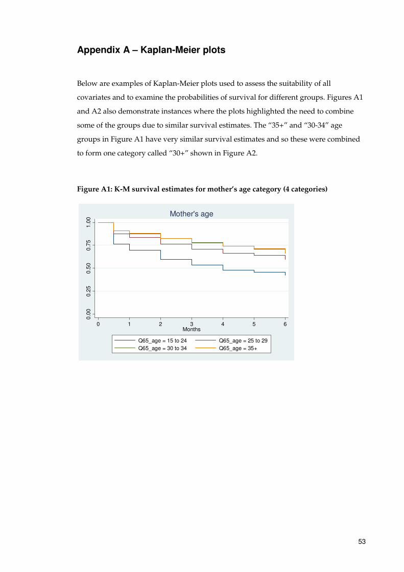
53

Appendix A – Kaplan-Meier plots

Below are examples of Kaplan-Meier plots used to assess the suitability of all

covariates and to examine the probabilities of survival for different groups. Figures A1

and A2 also demonstrate instances where the plots highlighted the need to combine

some of the groups due to similar survival estimates. The “35+” and “30-34” age

groups in Figure A1 have very similar survival estimates and so these were combined

to form one category called “30+” shown in Figure A2.

Figure A1: K-M survival estimates for mother’s age category (4 categories)

0.0

00

.25

0.5

00

.75

1.0

0

0 1 2 3 4 5 6Months

Q65_age = 15 to 24 Q65_age = 25 to 29

Q65_age = 30 to 34 Q65_age = 35+

Mother's age

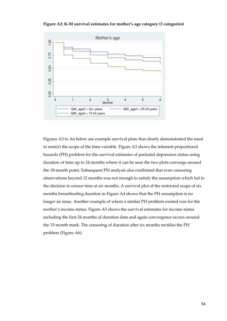
54

Figure A2: K-M survival estimates for mother’s age category (3 categories)

Figures A3 to A6 below are example survival plots that clearly demonstrated the need

to restrict the scope of the time variable. Figure A3 shows the inherent proportional

hazards (PH) problem for the survival estimates of perinatal depression status using

duration of time up to 24 months where it can be seen the two plots converge around

the 18-month point. Subsequent PH analysis also confirmed that even censoring

observations beyond 12 months was not enough to satisfy the assumption which led to

the decision to censor time at six months. A survival plot of the restricted scope of six

months breastfeeding duration in Figure A4 shows that the PH assumption is no

longer an issue. Another example of where a similar PH problem existed was for the

mother’s income status. Figure A5 shows the survival estimates for income status

including the first 24 months of duration data and again convergence occurs around

the 15-month mark. The censoring of duration after six months rectifies the PH

problem (Figure A6).

0.0

00

.25

0.5

00

.75

1.0

0

0 1 2 3 4 5 6Months

Q65_age2 = 30+ years Q65_age2 = 25-29 years

Q65_age2 = 15-24 years

Mother's age

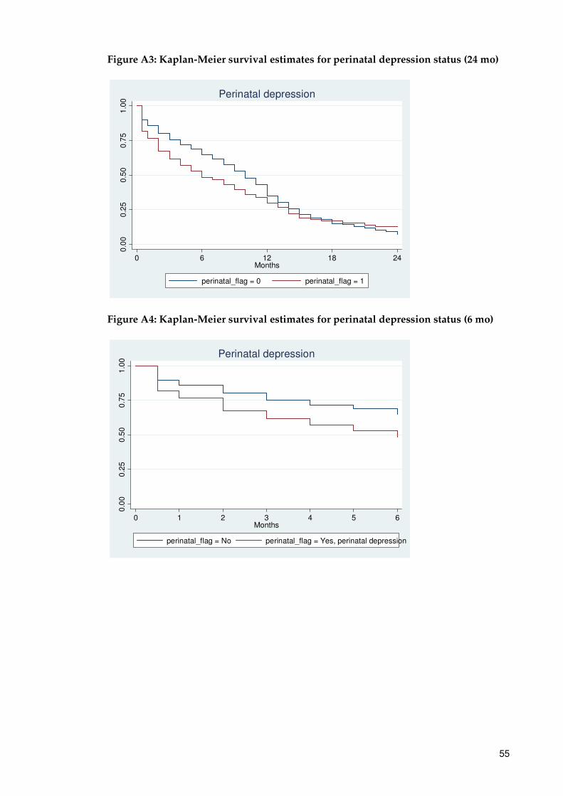
55

Figure A3: Kaplan-Meier survival estimates for perinatal depression status (24 mo)

Figure A4: Kaplan-Meier survival estimates for perinatal depression status (6 mo)

0.0

00

.25

0.5

00

.75

1.0

0

0 6 12 18 24Months

perinatal_flag = 0 perinatal_flag = 1


0.0

00

.25

0.5

00

.75

1.0

0

0 1 2 3 4 5 6Months

perinatal_flag = No perinatal_flag = Yes, perinatal depression


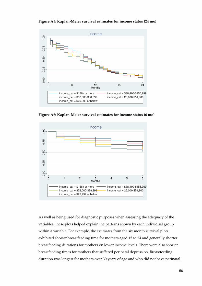
56

Figure A5: Kaplan-Meier survival estimates for income status (24 mo)

Figure A6: Kaplan-Meier survival estimates for income status (6 mo)

As well as being used for diagnostic purposes when assessing the adequacy of the

variables, these plots helped explain the patterns shown by each individual group

within a variable. For example, the estimates from the six month survival plots

exhibited shorter breastfeeding time for mothers aged 15 to 24 and generally shorter

breastfeeding durations for mothers on lower income levels. There were also shorter

breastfeeding times for mothers that suffered perinatal depression. Breastfeeding

duration was longest for mothers over 30 years of age and who did not have perinatal

0.0

00

.25

0.5

00

.75

1.0

0

0 6 12 18 24Months

income_cat = $156k or more income_cat = $88,400-$155,999

income_cat = $52,000-$88,399 income_cat = 26,000-$51,900

income_cat = $25,999 or below

Income

0.0

00

.25

0.5

00

.75

1.0

0

0 1 2 3 4 5 6Months

income_cat = $156k or more income_cat = $88,400-$155,999

income_cat = $52,000-$88,399 income_cat = 26,000-$51,900

income_cat = $25,999 or below

Income

57

depression. In terms of a mother’s income category, the risk of stopping breastfeeding

risk is highest in mothers with gross household incomes less than $26,000. The risk

decreases for each step up in income levels with those having gross household incomes

of over $156,000 having the lowest risk of stopping breastfeeding.

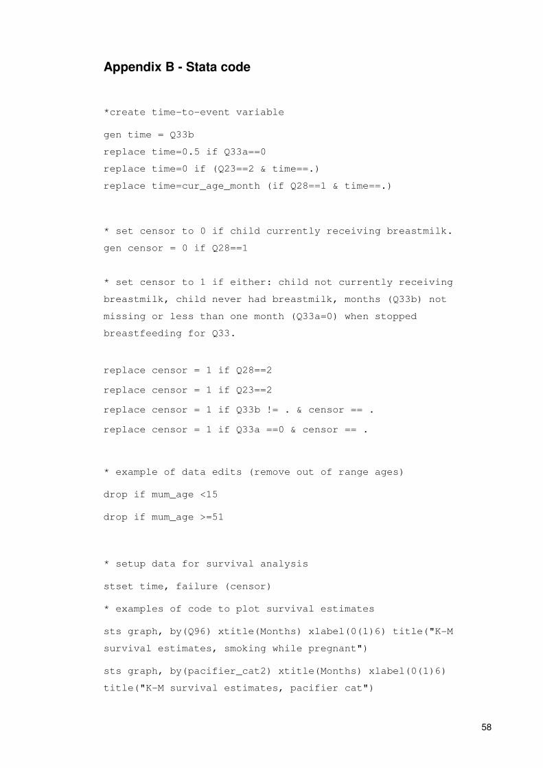
58

Appendix B - Stata code

*create time-to-event variable

gen time = Q33b

replace time=0.5 if Q33a==0

replace time=0 if (Q23==2 & time==.)

replace time=cur_age_month (if Q28==1 & time==.)

* set censor to 0 if child currently receiving breastmilk.

gen censor = 0 if Q28==1

* set censor to 1 if either: child not currently receiving

breastmilk, child never had breastmilk, months (Q33b) not

missing or less than one month (Q33a=0) when stopped

breastfeeding for Q33.

replace censor = 1 if Q28==2

replace censor = 1 if Q23==2

replace censor = 1 if Q33b != . & censor == .

replace censor = 1 if Q33a ==0 & censor == .

* example of data edits (remove out of range ages)

drop if mum_age <15

drop if mum_age >=51

* setup data for survival analysis

stset time, failure (censor)

* examples of code to plot survival estimates

sts graph, by(Q96) xtitle(Months) xlabel(0(1)6) title("K-M

survival estimates, smoking while pregnant")

sts graph, by(pacifier_cat2) xtitle(Months) xlabel(0(1)6)

title("K-M survival estimates, pacifier cat")

59

sts graph, by(seifa_quintile) xtitle(Months) xlabel(0(1)6)

title("K-M survival estimates, SEIFA quintiles")

sts graph, by(Q65_age) xtitle(Months) xlabel(0(1)6) title("K-M

survival estimates, mother's age")

stsatrisk, failure catrisk(0 (1) 6) tmax(12) ylab(0 (0.1) 0.80)

ytitle("Proportion stopped breastfeeding") xtitle("Duration of

breastfeeding (months)") scheme(s2mono) lspace(0.4) vspace(0.4)

title("Kaplan-Meier survival estimates")

* example of two-sample t test for characteristics table

ttest mum_age, by (receive_bm1)

* examples of tabulating characteristics for univariate analysis

tab ed_cat receive_bm, col

tab income_cat receive_bm, col

tab perinatal_flag receive_bm, col

* Table 4

tab Q10 Q22, row

* Table 5

tab remoteness Q22, row

* Table 7

xi: stcox i.Q10 i.Q65_age2 i.bmicat_now2 i.ed_3cat i.Q96_3cat

i.perinatal_flag i.Q17 i.Q25a_2cat i.Q13_2cat

* Table 8

xi: stcox i.Q96_3cat i.perinatal_flag i.Q17 i.Q13_2cat

* check collinearity

xi: stcox i.Q16 i.Q24

vif, uncentered

xi: stcox i.bmicat_b4 i.bmicat_now

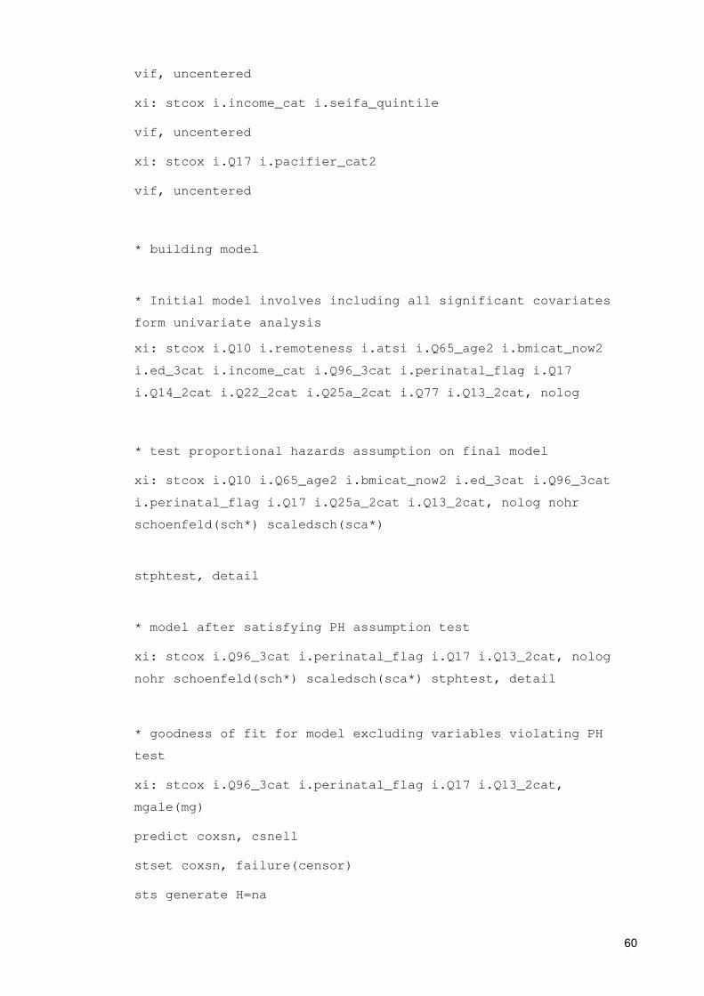
60

vif, uncentered

xi: stcox i.income_cat i.seifa_quintile

vif, uncentered

xi: stcox i.Q17 i.pacifier_cat2

vif, uncentered

* building model

* Initial model involves including all significant covariates

form univariate analysis

xi: stcox i.Q10 i.remoteness i.atsi i.Q65_age2 i.bmicat_now2

i.ed_3cat i.income_cat i.Q96_3cat i.perinatal_flag i.Q17

i.Q14_2cat i.Q22_2cat i.Q25a_2cat i.Q77 i.Q13_2cat, nolog

* test proportional hazards assumption on final model


i.perinatal_flag i.Q17 i.Q25a_2cat i.Q13_2cat, nolog nohr

schoenfeld(sch*) scaledsch(sca*)

stphtest, detail

* model after satisfying PH assumption test

xi: stcox i.Q96_3cat i.perinatal_flag i.Q17 i.Q13_2cat, nolog

nohr schoenfeld(sch*) scaledsch(sca*) stphtest, detail

* goodness of fit for model excluding variables violating PH

test

xi: stcox i.Q96_3cat i.perinatal_flag i.Q17 i.Q13_2cat,

mgale(mg)

predict coxsn, csnell

stset coxsn, failure(censor)

sts generate H=na

61

twoway (scatter H coxsn) (line coxsn coxsn)

stset time, failure(censor)

* goodness of fit for model including variables violating PH

test


i.perinatal_flag i.Q17 i.Q25a_2cat i.Q13_2cat, mgale(mg)

predict coxsn, csnell

stset coxsn, failure(censor)

sts generate H=na

twoway (scatter H coxsn) (line coxsn coxsn)

stset time, failure(censor)

* Figure 4

stsatrisk, failure catrisk(0 (1) 6) tmax(12) ylab(0 (0.1)

0.5,format(%3.1f)) ytitle("Proportion stopped breastfeeding")

xtitle("Duration of breastfeeding (months)") scheme(s2mono)

lspace(0.4) vspace(0.35) legend(label(1 "No regular pacifier use

(no)") label (2 "Regular pacifier use (yes)") pos(10) ring(0)

col(1)) title("Kaplan-Meier Survival Estimates")

* estimates of the failure functions for covariates from final

model

stsatrisk, by (Q17) failure catrisk(0 (1) 6) tmax(12) ylab(0

(0.1) 0.6, format(%3.1f)) ytitle("Proportion stopped

breastfeeding") xtitle("Duration of breastfeeding (months)")

scheme(s2mono) lspace(0.4) vspace(0.35) legend(label(1 "No

regular pacifier use (no)") label (2 "Regular pacifier use

(yes)") pos(10) ring(0) col(1)) title("Regular pacifier use")

stsatrisk, by (perinatal_flag) failure catrisk(0 (1) 6) tmax(12)

ylab(0 (0.1) 0.6, format(%3.1f)) ytitle("Proportion stopped


62

scheme(s2mono) lspace(0.4) vspace(0.35) legend(label(1 "No")

label (2 "Yes") pos(10) ring(0) col(1)) title("Perinatal

depression")

stsatrisk, by (Q96_3cat) failure catrisk(0 (1) 6) tmax(12)



scheme(s2mono) lspace(0.4) vspace(0.35) legend(label(1 "Not at

all") label (2 "Weekly or less") label (3 "Daily") pos(10)

ring(0) col(1)) title("Smoking while pregnant")

stsatrisk, by (Q13_2cat) failure catrisk(0 (1) 6) tmax(12)



scheme(s2mono) lspace(0.4) vspace(0.35) legend(label(1

"Vaginal") label (2 "Caesarean") pos(10) ring(0) col(1))

title("Child delivery method")

63

This page is intentionally left blank

Documents

Workplace Project Portfolio C (WPP C)