Workload-Aware Resource Sharing and Cache Management …nabil/pub/Workload_Aware_TechReport07.pdf · Workload-Aware Resource Sharing and Cache Management for Scalable Video Streaming

Workload-Aware Resource Sharing and CacheManagement for Scalable Video Streaming

Bashar Qudah Nabil J. SarhanThe Department of Electrical and Computer Engineering

Wayne State UniversityDetroit, MI, 48202 USA

e-mail: {bqudah,nabil}@wayne.edu

October 22, 2007

Part of the paper was presented at MASCOTS 2006.This work is supported in part by NSF grant CNS-0626861.

1

Abstract

The required real-time and high-rate transfers for multimedia data severelylimit the number of requests that can be serviced by Video-on-Demand(VOD) servers. Resource sharing techniques can be used to address thisproblem. We evaluate through extensive simulation major resource shar-ing techniques from different classes, considering both the True Video-on-Demand (TVOD) and Near Video-on-Demand (NVOD) service models. TheTVOD model helps in analyzing the server communication bandwidth anddisk I/O bandwidth requirements, whereas the NVOD model helps in com-paring the achieved throughput, waiting times, and unfairness towards un-popular videos. We utilize this extensive analysis in developing a workloadaware hybrid solution (WAHS) that combines the advantages of the bestamong resource sharing techniques. Moreover, we propose a statistical cachemanagement approach (SCM) and derive analytical models for optimal cacheallocation to reduce the demands on the disk I/O when various resource shar-ing techniques are used.

0.1 Introduction

Video-on-Demand (VOD), though has been around for a while as an alterna-tive delivery method, is advancing slowly but surely towards a more marketshare, and is expected to exceed that of broadcast-based TV programmingand DVD movie rentals at stores. The main driving forces behind this phe-nomena are the increasing expectations of viewers as new generations enterthe market, and the industry interest in more control and lower cost of thedelivery process. However, the pace of this advancement is decided by thequality and speed of solutions in the face of the main challenges.

In the technical side, the challenges are greater and harder to solve, themore popular VOD becomes. The number of concurrent video streams thatcan be supported by a VOD server is highly constrained by the required real-time and high-rate transfers. These requirements quickly consume serverresources, including network bandwidth and disk I/O bandwidth.

Resource sharing techniques face this challenge by utilizing the mul-ticast facility. Two resource sharing paradigms dominate scalable videostreaming; stream merging [21, 5, 11, 29, 3, 27, 28] and periodic broadcasting[14, 20, 22, 24, 23, 2, 33, 32]. Stream merging techniques combine streamswhen possible to reduce the delivery costs. These techniques include Patch-ing [6, 21], Transition Patching [5, 7], and Earliest Reachable Merge Tar-get (ERMT) [11, 13]. Periodic broadcasting techniques, such as SkyscraperBroadcasting (SB) [22], Greedy Disk-conserving Broadcasting (GDB) [14],Harmonic Broadcasting (HB) [24], and Fibonacci Broadcasting (FB) [20],divide each supported video into multiple segments and broadcast them pe-riodically on dedicated channels. While stream merging suits wider spectrumof video workloads, periodic broadcasting can be more efficient in serving theextremely popular videos. The decision which paradigm to follow and whichtechnique to use has a great impact on the system overall performance andthroughput, and on the quality of service perceived by clients.

Though efforts have been spent on designing and optimizing techniques ineach group, the option of utilizing both at the same time was not consideredbeyond a casual mentioning, either to justify the need for another periodicbroadcasting technique, or at best arbitrarily by serving some popular videosin the system by a periodic broadcasting technique without a clear criteriaon how to choose them. Selective Catching [16] (and Catching [16]) is an ex-ception to this general pattern, but it suffers from two main problems. First,as we demonstrate in this paper, the chosen techniques to mix are not the

1

best each group can offer. Second, modifying a periodic broadcasting tech-nique to fit a stream merging like behavior causes the periodic broadcastingtechnique to lose its source of strength.

To start with, the literature lacks detailed comparative analysis of variousresource sharing strategies. With the many available resource sharing tech-niques from different classes, it is unclear which one is the best to use in atarget environment. For example, it is unclear how ERMT performs in com-parison with Selective Catching and Transition Patching and how periodicbroadcasting techniques perform compared with stream merging techniques.Moreover, only limited performance metrics, workloads, and service modelswere considered.

Furthermore, there is very little work on cache management for reducingthe demands on the disk I/O when resource sharing techniques are applied.This is, however, an important issue for designing cost effective and scalableVOD servers, especially because of the widening gap between technologyimprovements in the capacities and speeds of hard disk drives [18]. In [4],the impact of caching was reported by actual measurements for only limitedcaching schemes and limited and simple resource sharing techniques. Theresults show that without caching, the disk I/O bandwidth may become abottleneck.

This paper addresses those limitations. The main contributions of thisstudy can be summarized as follows.

• We evaluate through extensive simulation major resource sharing tech-niques under both the True Video-on-Demand (TVOD) and Near Video-on-Demand (NVOD) service models and for two target workloads, oneconsisting of videos with varying popularities and the other consistingof only popular videos.

• We propose a new workload aware hybrid solution (WAHS) that com-bines the advantages of the best in stream merging and periodic broad-casting techniques. The solution is armed with a dynamic configurationalgorithm capable of responding to any significant change in the work-load or the system available resources, and it is tuned for high serverthroughput.

• We propose a statistical cache management approach (SCM). With thisapproach, the server periodically computes video access frequencies anddetermines the data to be cached based on these statistics. Besides

2

being performance effective, this approach is easy to implement andincurs small overhead as updates are triggered only when the work-load varies considerably. We derive analytical models for allocatingcache space for various resource sharing techniques. This work differssignificantly from previous work on proxy caching [25] (and referenceswithin), which has different objectives and factors affecting the alloca-tion decisions. In addition, our approach differs from low-level cachingtechniques, such as Least Recently Used (LRU), Least Frequently Used(LFU), and Interval Caching [8, 30], whereby the content of the cachechanges frequently, incurring significant overheads. SCM is comparedto Interval Caching [9] and is shown to achieve significantly better per-formance when implemented with the most aggressive resource sharingtechniques.

• We develop analytical models for optimal tuning of design parametersfor Transition Patching and Selective Catching.

• We introduce the load on the underlying storage subsystem as an ad-ditional dimension to the comparisons among various resource sharingtechniques and examine the impact of caching on reducing these re-quirements.

The performance evaluation considers four target environments: mixed-video workload and TVOD, hot-video workload and TVOD, mixed-video work-load and NVOD, and hot-video workload and NVOD. While the mixed-videoenvironments are more realistic, the hot-video environments are used to an-alyze periodic broadcasting that are designed for popular videos. In TVOD,we compare the server resources required to service all requests immediately.In NVOD, however, we fix server resources and compare the number of cus-tomers that can be serviced concurrently, the waiting times, and unfairnesstowards unpopular videos. This study examines the impacts of many sys-tem and workload parameters, including customer waiting tolerance, requestarrival rate, number of videos, server network bandwidth, and cache size.The effect of request scheduling is also discussed. Furthermore, we intro-duce and apply a framework for comparing periodic broadcasting techniqueswith other techniques. We consider here the ability of periodic broadcastingtechniques to limit the maximum waiting time and to provide waiting timeguarantees.

3

The rest of this paper is organized as follows. Section 0.2 discusses majorresource sharing techniques and cache management. WAHS, the proposedhybrid solution is presented in Section 0.3, and SCM, the proposed cachemanagement approach is presented in Section 0.4. Section 0.5 shows howdesign parameters can be tuned optimally. Section 0.6 discusses the per-formance evaluation methodology and workload characteristics and presentsthe main results. Finally, conclusions are drawn in the last section.

0.2 Background Information

0.2.1 Resource sharing

Let us now discuss the main resource sharing techniques analyzed in thepaper: Patching, Transition Patching, ERMT, Selective Catching, FB, SB,GDB, and HB. This study excludes techniques that achieve low resource shar-ing (such as Batching[10]) or reduce playback quality (such as Piggybacking[17]). To conduct fair comparisons and account for limitations in client band-width, we do not consider techniques that require client download bandwidthmore than double the video playback rate, except for Harmonic Broadcasting(HB). Despite requiring high download bandwidth in the client, HB is veryeffective in reducing the required server bandwidth. In addition, we excludetechniques that are designed for heterogeneous receivers such as EnhancedHybrid Solution (EHS) [27], HeRo [2], BroadCatch [33], and Optimized Het-erogeneous Periodic Broadcasting (OHPB) [32] for losing their advantagesin homogeneous environments and performing similar or worse than theircounterpart techniques that are designed for homogeneity.

Stream Merging Techniques

While Batching services all waiting requests for a video using one full multi-cast video stream and requires only one client download channel at the videoplayback rate. Patching expands the multicast tree dynamically to includenew requests. A new request joins the latest regular (i.e., full) stream for theobject and receives the missing portion as a patch. Hence, it requires twodownload channels (each at the video playback rate) and additional clientbuffer space. When the playback of the patch is completed, the client contin-ues the playback of the remaining portion using the data received from the

4

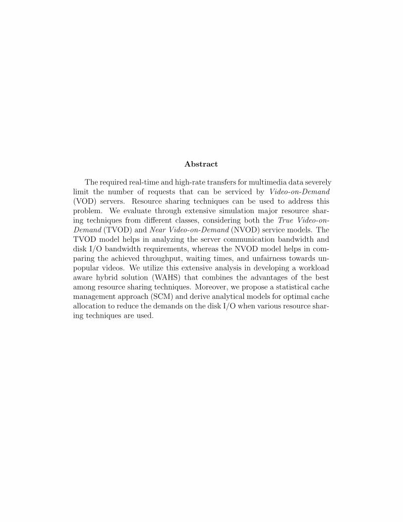
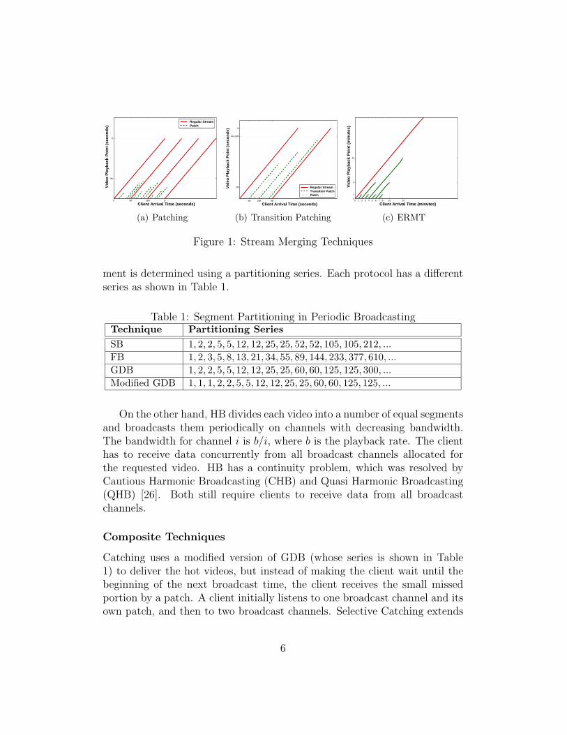
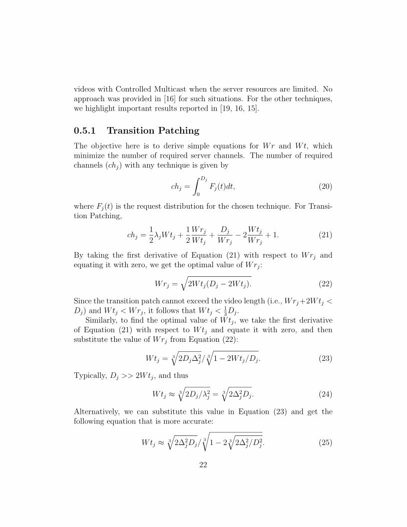
multicast stream and already buffered locally. To avoid the continuously in-creasing patch lengths, regular streams are retransmitted when the requiredpatch length exceeds a pre-specified value called regular window (Wr). Fig-ure 1(a) further explains the concept in servicing one video of D seconds inlength. (Typically, Wr is much smaller than D.)

Transition Patching allows some patches to be sharable by extending theirlengths. It introduces another multicast stream, called transition patch. Thethreshold to start a regular stream is Wr as in Patching, and the threshold tostart a transition patch is called the transition window (Wt). The transitionpatch length is equal to the difference between the starting times of thetransition patch and the last regular stream plus 2Wt, whereas the length ofthe patch is equal to the difference between the starting times of the patchand the latest transition stream or regular stream. Hence, the maximumpossible patch length is Wt, and the maximum possible transition patchlength is Wr + 2Wt. Figure 1(b) further illustrates the concept. A possiblescenario for a client is to start listening to its own patch and the transitionpatch, and when its patch is completed, it starts listening to the regularstream.

ERMT is a near optimal hierarchical stream merging technique. It alsorequires two download channels (each at the playback rate), but it makes eachstream sharable and thus leads to a dynamic merge tree. A new client joinsthe closest reachable stream (target) and receives the missing portion by anew stream (merger). Reachable means the merge can occur before the targetterminates. After the merger stream finishes and merges into the target,the later can get extended to satisfy the playback requirement of the newclient(s), and this extension can affect its own merge target. For example,in Figure 1(c), the third stream length got extended from two minutes tofour minutes after the fourth stream had merged with it. ERMT is used byBandwidth Skimming [12] to work when the client download bandwidth isless than double the playback rate.

Periodic Broadcasting Techniques

SB, GDB, and FB divide each video into a number of non-equal segmentsand broadcast each segment periodically on a dedicated channel at the videoplayback rate. The client waits until the beginning of the next broadcastof the first segment and then receives data concurrently from two broadcastchannels. The relative length of the nth segment compared to the first seg-

5

0 Wr 2Wr D

Wr

D

Vid

eo P

layb

ack

Po

int

(sec

on

ds)

Client Arrival Time (seconds)

Regular Stream Patch

(a) Patching

Wt 2Wt Wr

Wt

Wr+2Wt

D

Vid

eo P

layb

ack

Po

int

(sec

on

ds)

Client Arrival Time (seconds)

Regular Stream Transition Patch Patch

(b) Transition Patching

0 1 2 3 4 5 6 7 8 10 140

1

4

10

Vid

eo P

layb

ack

Po

int

(min

ute

s)

Client Arrival Time (minutes)

(c) ERMT

Figure 1: Stream Merging Techniques

ment is determined using a partitioning series. Each protocol has a differentseries as shown in Table 1.

Table 1: Segment Partitioning in Periodic BroadcastingTechnique Partitioning SeriesSB 1, 2, 2, 5, 5, 12, 12, 25, 25, 52, 52, 105, 105, 212, ...

FB 1, 2, 3, 5, 8, 13, 21, 34, 55, 89, 144, 233, 377, 610, ...

GDB 1, 2, 2, 5, 5, 12, 12, 25, 25, 60, 60, 125, 125, 300, ...

Modified GDB 1, 1, 1, 2, 2, 5, 5, 12, 12, 25, 25, 60, 60, 125, 125, ...

On the other hand, HB divides each video into a number of equal segmentsand broadcasts them periodically on channels with decreasing bandwidth.The bandwidth for channel i is b/i, where b is the playback rate. The clienthas to receive data concurrently from all broadcast channels allocated forthe requested video. HB has a continuity problem, which was resolved byCautious Harmonic Broadcasting (CHB) and Quasi Harmonic Broadcasting(QHB) [26]. Both still require clients to receive data from all broadcastchannels.

Composite Techniques

Catching uses a modified version of GDB (whose series is shown in Table1) to deliver the hot videos, but instead of making the client wait until thebeginning of the next broadcast time, the client receives the small missedportion by a patch. A client initially listens to one broadcast channel and itsown patch, and then to two broadcast channels. Selective Catching extends

6

Catching by delivering the cold videos using Controlled Multicast [15], whichworks essentially the same as Patching.

0.2.2 Cache Management

Interval caching exploits the high skewness in video access patterns by cachingintervals between successive streams accessing the same contents in the mainmemory of the server. Specifically, interval caching reuses the data broughtby a stream in servicing a closely following stream if sufficient cache spaceexists to hold the data blocks in the cache. The two streams are calledthe following stream and the preceding stream, respectively. The followingstream will have to be serviced from disks until the playback reaches the firstcached block. The required cache space for servicing the following streamdepends on the time interval between the two streams and the compressionmethod used. Interval caching uses the cache (memory) space efficiently byvictimizing longer intervals for caching shorter ones.

0.3 Workload Aware Hybrid Solution (WAHS)

Two resource sharing paradigms dominate scalable video streaming; streammerging and periodic broadcasting. While the former suits wider spectrum ofvideo workloads, the later can be more efficient in serving extremely popularvideos. The decision on which paradigm to follow and which technique touse has a great impact on the system overall performance and throughput,and on the quality of service perceived by clients.

Though efforts have been spent on designing and optimizing techniques ineach group, the option of utilizing both at the same time was not consideredbeyond a casual mentioning, either to justify the need for another periodicbroadcasting technique, or at best arbitrarily by serving some popular videosin the system by a periodic broadcasting technique without a clear criteriaon how to choose them. Selective Catching [16] (and Catching [16]) is an ex-ception to this general pattern, but it suffers from two main problems. First,as we demonstrate in this paper, the chosen techniques to mix are not thebest each group can offer. Second, modifying a periodic broadcasting tech-nique to fit a stream merging like behavior causes the periodic broadcastingtechnique to lose its source of strength. As we show later in this paper, Se-lective Catching performs worse than some of the efficient stream merging

7

techniques without even adding any periodic broadcasting componenet tothem.

We propose a workload aware hybrid solution (WAHS) that provides clearapproaches for answering all key configuration questions. The configurationof the system is not static but dynamic and responds to any significant changein the workload or the available system resources. The solution combines thebest in each group (as will be shown in Section 0.6), ERMT as the streammerging technique with Fibonacci periodic broadcasting. Fibonacci is usedfor the most popular videos while ERMT is used for the remaining. Howeverthe Hybrid solution might dynamically converge under certain conditions toone of the two techniques when that potentially achieves better performance.Such as a combination of very low request rate and limited server resourcesmight lead to pure ERMT. But in general, the decision is more involving andneeds to take into consideration several factors at once and to response tochanges dynamically, as well. The main three configuration parameters theapproach tries to set optimally are: (1) How many videos to serve using eachtechnique? (2) How to split the available resources between the two groupsof service? (3) And how to distribute the resources reserved for the broad-casting group among the broadcasting videos for best possible performance?Within the ERMT group the resources are shared by requests of all videosin the group and managed by the scheduling policy in place. The hybridsolution is primarly tuned by the configuration process for higher through-put then for lower average customer waiting time. However the order canbe easily interchanged if desired. Another issue, while system resources in-clude more than server network channels ChAva, such as the I/O channelsand the cache space, for their exceptional importance and simplicity, servernetwork channels are the primary focus in the discussion below. However,other resources can be included in the decision process as needed.

0.3.1 Step I: Forming The Two Groups

The first step in this direction is deciding whether forming two groups is abetter choice. Given the expected workload, customer waiting and defectionbehavior, and the level of resources the system does allocate for service, canERMT provide a TVOD service on its own? If yes, problem is solved andno need for hybridizing till conditions are changed. However, if the answer isno, another question needs to be answered. Is Fibonacci capable of providinga zero-defection (0-D) service by itself? If answer is yes, again problem is

8

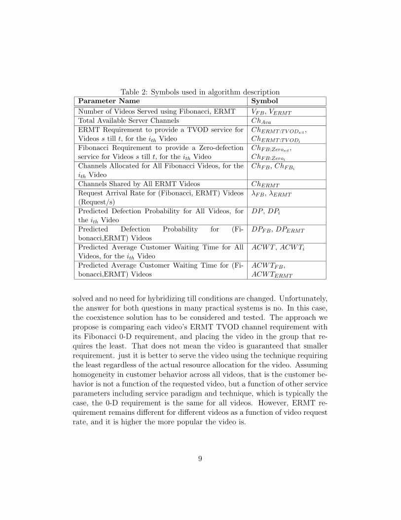
Table 2: Symbols used in algorithm descriptionParameter Name SymbolNumber of Videos Served using Fibonacci, ERMT VFB, VERMT

Total Available Server Channels ChAva

ERMT Requirement to provide a TVOD service forVideos s till t, for the ith Video

ChERMT :TV ODs:t ,ChERMT :TV ODi

Fibonacci Requirement to provide a Zero-defectionservice for Videos s till t, for the ith Video

ChFB:Zeros:t ,ChFB:Zeroi

Channels Allocated for All Fibonacci Videos, for theith Video

ChFB, ChFBi

Channels Shared by All ERMT Videos ChERMT

Request Arrival Rate for (Fibonacci, ERMT) Videos(Request/s)

λFB, λERMT

Predicted Defection Probability for All Videos, forthe ith Video

DP , DPi

Predicted Defection Probability for (Fi-bonacci,ERMT) Videos

DPFB, DPERMT

Predicted Average Customer Waiting Time for AllVideos, for the ith Video

ACWT , ACWTi

Predicted Average Customer Waiting Time for (Fi-bonacci,ERMT) Videos

ACWTFB,ACWTERMT

solved and no need for hybridizing till conditions are changed. Unfortunately,the answer for both questions in many practical systems is no. In this case,the coexistence solution has to be considered and tested. The approach wepropose is comparing each video’s ERMT TVOD channel requirement withits Fibonacci 0-D requirement, and placing the video in the group that re-quires the least. That does not mean the video is guaranteed that smallerrequirement. just it is better to serve the video using the technique requiringthe least regardless of the actual resource allocation for the video. Assuminghomogeneity in customer behavior across all videos, that is the customer be-havior is not a function of the requested video, but a function of other serviceparameters including service paradigm and technique, which is typically thecase, the 0-D requirement is the same for all videos. However, ERMT re-quirement remains different for different videos as a function of video requestrate, and it is higher the more popular the video is.

9

Predicting ERMT TVOD Requirement

The ERMT TVOD requirement to serve all V videos can be predicted usingthe following:

ChERMT :TV OD1:V=

V∑i=1

ChERMT :TV ODi. (1)

Since all videos actually share the pool of resources in case of ERMT, there-fore, when the number of videos are large enough (which is typically thecase), ChERMT :TV ODi

can be substitute with the average server channel re-quirement for the ith video (versus the actual or maximum requirement),which can be predicted using [12]:

ChERMT :TV ODi= η ∗ log(λi × Di/η), (2)

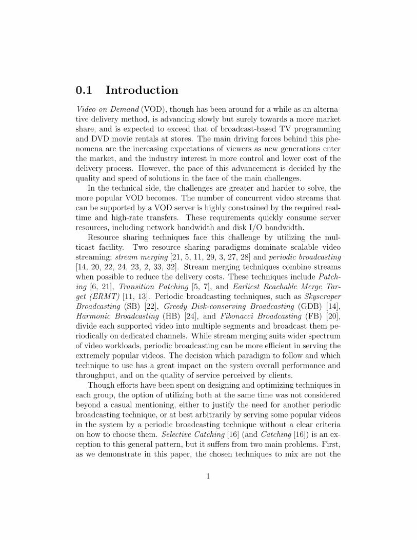
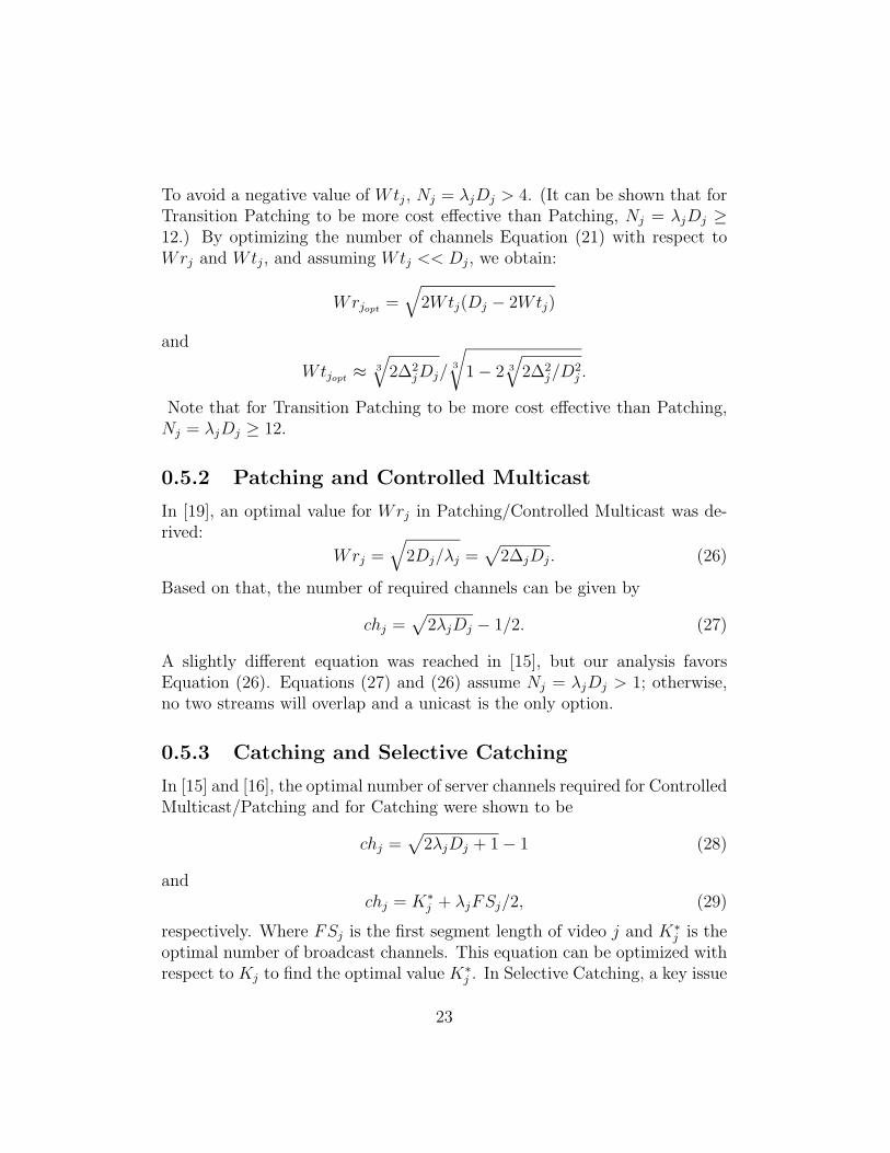
where λi is the request arrival rate (request/second), and Di is the durationin seconds of the ith video. η found by [12] to be 1.62 for an optimal streammerging technique requiring two channels in the client side. However, sinceERMT is not the optimal off-line technique η = 1.62 was derived for, but itis the best known practical on-line stream merging technique, a higher valueof η is required. As presented in Figure 2(a), we found experimentally thatη = 2.0 works better for ERMT.

Predicting Fibonacci 0-D Requirement

Fibonacci 0-D channel requirement per video is independent from video re-quest rate, but depends solely on customer defection behavior. What isrequired is a cap on the maximum waiting time (first segment length) belowthe customer waiting tolerance that with time of service guarantee, which Fi-bonacci is capable of providing, results in almost zero-defection. Once thatvalue is known, the required number of channels are easy to calculate, toresult in a first segment of shorter length.

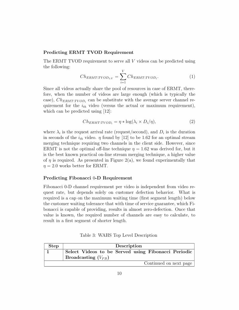
Table 3: WAHS Top Level Description

Step Description1 Select Videos to be Served using Fibonacci Periodic

Broadcasting (VFB)Continued on next page

10

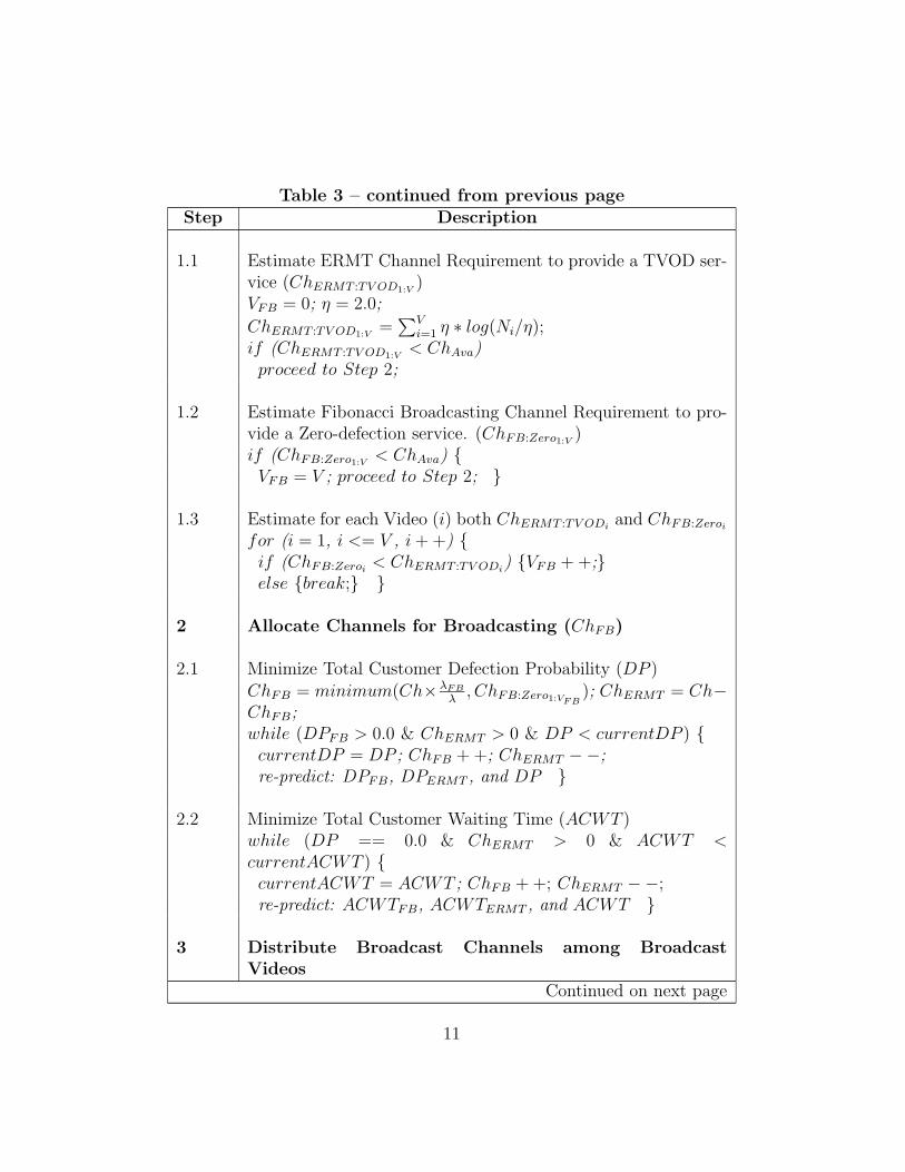
Table 3 – continued from previous pageStep Description

1.1 Estimate ERMT Channel Requirement to provide a TVOD ser-vice (ChERMT :TV OD1:V

)VFB = 0; η = 2.0;

ChERMT :TV OD1:V=

∑Vi=1 η ∗ log(Ni/η);

if (ChERMT :TV OD1:V< ChAva)

proceed to Step 2;

1.2 Estimate Fibonacci Broadcasting Channel Requirement to pro-vide a Zero-defection service. (ChFB:Zero1:V

)if (ChFB:Zero1:V

< ChAva) {VFB = V ; proceed to Step 2; }

1.3 Estimate for each Video (i) both ChERMT :TV ODiand ChFB:Zeroi

for (i = 1, i <= V , i + +) {if (ChFB:Zeroi

< ChERMT :TV ODi) {VFB + +;}

else {break;} }

2 Allocate Channels for Broadcasting (ChFB)

2.1 Minimize Total Customer Defection Probability (DP )ChFB = minimum(Ch× λFB

λ, ChFB:Zero1:VFB

); ChERMT = Ch−ChFB;while (DPFB > 0.0 & ChERMT > 0 & DP < currentDP ) {currentDP = DP ; ChFB + +; ChERMT −−;re-predict: DPFB, DPERMT , and DP }

2.2 Minimize Total Customer Waiting Time (ACWT )while (DP == 0.0 & ChERMT > 0 & ACWT <currentACWT ) {currentACWT = ACWT ; ChFB + +; ChERMT −−;re-predict: ACWTFB, ACWTERMT , and ACWT }

3 Distribute Broadcast Channels among BroadcastVideos

Continued on next page

11

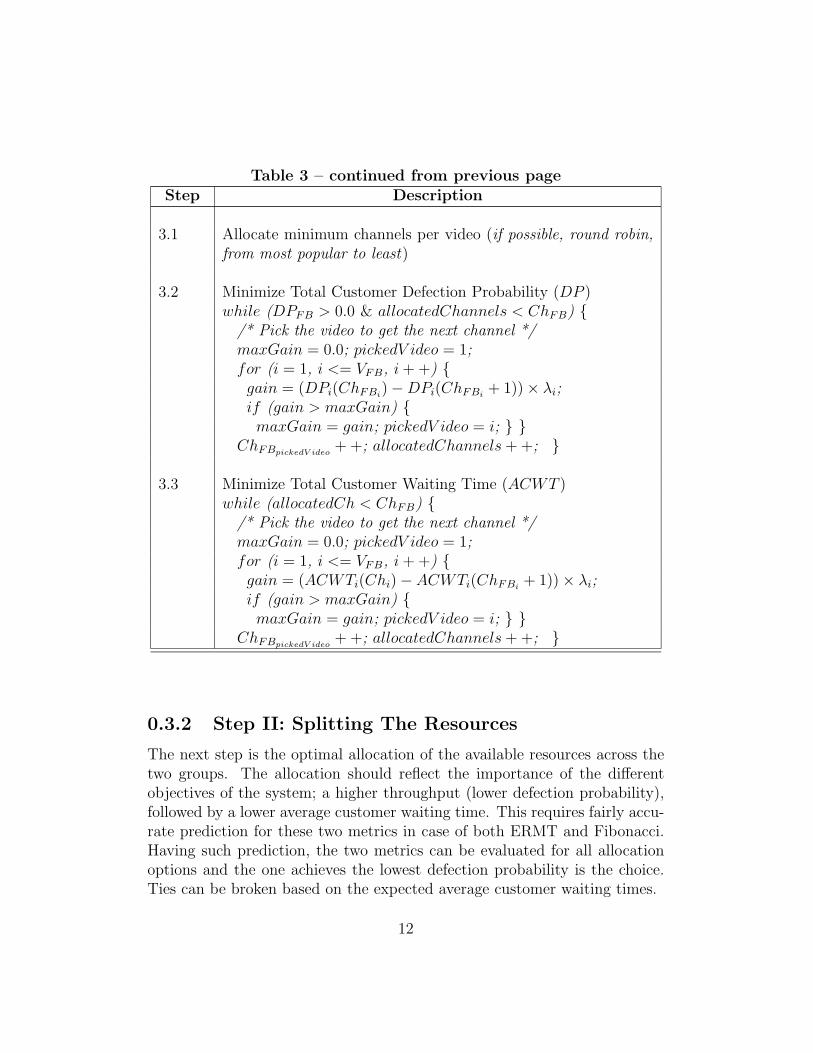
Table 3 – continued from previous pageStep Description

3.1 Allocate minimum channels per video (if possible, round robin,from most popular to least)

3.2 Minimize Total Customer Defection Probability (DP )while (DPFB > 0.0 & allocatedChannels < ChFB) {

/* Pick the video to get the next channel */maxGain = 0.0; pickedV ideo = 1;for (i = 1, i <= VFB, i + +) {gain = (DPi(ChFBi

) − DPi(ChFBi+ 1)) × λi;

if (gain > maxGain) {maxGain = gain; pickedV ideo = i; } }

ChFBpickedV ideo+ +; allocatedChannels + +; }

3.3 Minimize Total Customer Waiting Time (ACWT )while (allocatedCh < ChFB) {

/* Pick the video to get the next channel */maxGain = 0.0; pickedV ideo = 1;for (i = 1, i <= VFB, i + +) {gain = (ACWTi(Chi) − ACWTi(ChFBi

+ 1)) × λi;if (gain > maxGain) {maxGain = gain; pickedV ideo = i; } }

ChFBpickedV ideo+ +; allocatedChannels + +; }

0.3.2 Step II: Splitting The Resources

The next step is the optimal allocation of the available resources across thetwo groups. The allocation should reflect the importance of the differentobjectives of the system; a higher throughput (lower defection probability),followed by a lower average customer waiting time. This requires fairly accu-rate prediction for these two metrics in case of both ERMT and Fibonacci.Having such prediction, the two metrics can be evaluated for all allocationoptions and the one achieves the lowest defection probability is the choice.Ties can be broken based on the expected average customer waiting times.

12

The overall predicted defection probability (DP ) and average customerwaiting time (ACWT ) can be calculated by the weighted averages of thecorresponding group level metrics:

DP = DPFB × λFB

λ+ DPERMT × λERMT

λ, (3)

and

ACWT = ACWTFB × λFB

λ+ ACWTERMT × λERMT

λ. (4)

Predicting Fibonacci Metrics: DPFB and ACWTFB

Fibonacci group level metrics; DPFB and ACWTFB, can be calculated intheir turn by the weighted averages of the corresponding video level metrics::

DPFB =

VFB∑i=1

DPi × λi

λFB

(5)

and

ACWTFB =

VFB∑i=1

ACWTi × λi

λFB

. (6)

The real challenge is in predicting the video level metrics. The video leveldefection probability, in case of Fibonacci, is a function of the customer wait-ing and defection model and the channels allocated for the video. The firstsegment length (li) can be easily calculated based on the available channels,which represents the maximum waiting time for any customer requesting thatparticular video. Assuming equal probability for request arrival during thatperiod (which is typically usually the case) Then DPi can be calculated by:

DPi =

∫ li

0

F (x).dx, (7)

where F (x) is the cumulative distribution function of the customer waitingtolerence model (i.e. F (x) is the probability the customer maximum waitingtime is ≤ x). The customer waiting tolerence model can be built statisti-cally based on system historical information. However, the video allocatedchannels is not known yet. The number of videos in the group is known fromStep I, and the above sub-process is executed for an assumed group chan-nel allocation, therefore, distributing the examined group channel allocation

13

among the group videos is required to know the assumed video allocatedchannels. One trivial solution is to distribute the channels equally amongthe group videos, however a more optimal solution is explained in Step III.The distribution algorithm need to be executed iteratively in Step II beforeit is finally executed for the actual group allocation; the output of Step 2.The video level average customer waiting time is much easier and a functionof only the video channel allocation. Simply, ACWTi = li/2. Figure 2(b)demonstrates how accurate the predition of the defection rate is in case ofFibonacci.

Predicting ERMT Metrics: DPERMT and ACWTERMT

Unlike Fibonacci, the ERMT group level metrics are harder to predict. Theresource pooling, scheduling policy interaction, the dependency on the re-quest rate, and the dynamic nature of the technique, all make predictioncomplex and hard with stream merging techniques, and ERMT is no excep-tion. Though ERMT does not isolate videos during service, but to simplifythis complexity, we follow the divide and conquer approach by performingthe prediction at the video level, as we did with Fibonacci. Therefore, asin Fibonacci, the group level metrics; DPERMT and ACWTERMT , are cal-culated in their turn by weighted averages of the corresponding video levelmetrics::

DPERMT =V∑

i=VFB+1

DPi × λi

λERMT

(8)

and

ACWTERMT =V∑

i=VFB+1

ACWTi × λi

λERMT

. (9)

However a series of modifications are introduced to fit that approach for theERMT case.

The first modification is in predicting the video actual average share ofchannels. Though the resources are pooled with ERMT, but practically ata snapshot of time the channels has to be allocated for the different videorequests managed by the scheduling policy. We try to predict the averageshare over long period of time, but that lack the accuracy in case of Fibonacci,where the allocation is static and known in advance. Under a fair schedulingpolicy like FCFS, each video is expected to receive in average a share of

14

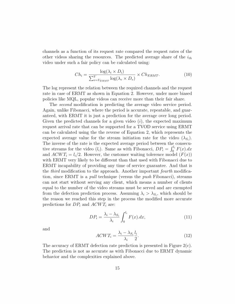
channels as a function of its request rate compared the request rates of theother videos sharing the resources. The predicted average share of the ithvideo under such a fair policy can be calculated using:

Chi =log(λi × Di)∑V

v=VERMTlog(λv × Dv)

× ChERMT . (10)

The log represent the relation between the required channels and the requestrate in case of ERMT as shown in Equation 2. However, under more biasedpolicies like MQL, popular videos can receive more than their fair share.

The second modification is predicting the average video service period.Again, unlike Fibonacci, where the period is accurate, repeatable, and guar-anteed, with ERMT it is just a prediction for the average over long period.Given the predicted channels for a given video (i), the expected maximumrequest arrival rate that can be supported for a TVOD service using ERMTcan be calculated using the the reverse of Equation 2, which represents theexpected average value for the stream initiation rate for the video (λSi

).The inverse of the rate is the expected average period between the consecu-tive streams for the video (li). Same as with Fibonacci, DPi =

∫ li0

F (x).dxand ACWTi = li/2. However, the customer waiting tolerence model (F (x))with ERMT very likely to be different than that used with Fibonacci due toERMT incapability of providing any time of service guarantee. And that isthe third modification to the approach. Another important fourth modifica-tion, since ERMT is a pull technique (versus the push Fibonacci), streamscan not start without serving any client, which means a number of clientsequal to the number of the video streams must be served and are exemptedfrom the defection prediction process. Assuming λi > λSi

, which should bethe reason we reached this step in the process the modified more accuratepredictions for DPi and ACWTi are:

DPi =λi − λSi

λi

∫ li

0

F (x).dx, (11)

and

ACWTi =λi − λSi

λi

li2. (12)

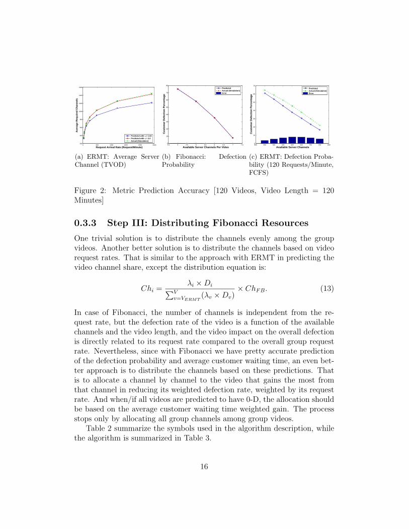
The accuracy of ERMT defection rate prediction is presented in Figure 2(c).The prediction is not as accurate as with Fibonacci due to ERMT dynamicbehavior and the complexities explained above.

15

0 500 1000 1500 2000 2500200

400

600

800

1000

1200

1400

1600

Request Arrival Rate (Request/Minute)

Ave

rag

e R

equ

ired

Ch

ann

els

Predicted with η = 1.62 Predicted with η = 2.0 Actual (Simulation)

(a) ERMT: Average ServerChannel (TVOD)

3.5 4 4.5 5 5.5 6 6.5 7 7.50

10

20

30

40

50

60

70

80

Available Server Channels Per Video

Cu

sto

mer

Def

ecti

on

Per

cen

tag

e

Predicted Actual (Simulation) Error

(b) Fibonacci: DefectionProbability

400 450 500 550 600 650 700 750 8000

10

20

30

40

50

60

70

Available Server Channels

Cu

sto

mer

Def

ecti

on

Per

cen

tag

e

Predicted Actual (Simulation) Error

(c) ERMT: Defection Proba-bility (120 Requests/Minute,FCFS)

Figure 2: Metric Prediction Accuracy [120 Videos, Video Length = 120Minutes]

0.3.3 Step III: Distributing Fibonacci Resources

One trivial solution is to distribute the channels evenly among the groupvideos. Another better solution is to distribute the channels based on videorequest rates. That is similar to the approach with ERMT in predicting thevideo channel share, except the distribution equation is:

Chi =λi × Di∑V

v=VERMT(λv × Dv)

× ChFB. (13)

In case of Fibonacci, the number of channels is independent from the re-quest rate, but the defection rate of the video is a function of the availablechannels and the video length, and the video impact on the overall defectionis directly related to its request rate compared to the overall group requestrate. Nevertheless, since with Fibonacci we have pretty accurate predictionof the defection probability and average customer waiting time, an even bet-ter approach is to distribute the channels based on these predictions. Thatis to allocate a channel by channel to the video that gains the most fromthat channel in reducing its weighted defection rate, weighted by its requestrate. And when/if all videos are predicted to have 0-D, the allocation shouldbe based on the average customer waiting time weighted gain. The processstops only by allocating all group channels among group videos.

Table 2 summarize the symbols used in the algorithm description, whilethe algorithm is summarized in Table 3.

16

0.4 Statistical Cache Management (SCM)

The goal of cache management is to reduce the load on the storage subsystemand thus reduce the cost of the overall solution by caching selected data in themain memory. While Interval Caching [8] shown to be effective in reducingthe I/O requirements when applied with Batching, it does not address byitself the problem of the limited network bandwidth and its effectiveness wasnot evaluated with more aggressive resource sharing techniques. Besides itcan incur significant overhead on the system.

We investigate here a statistical approach for cache management. Withthis approach, the server periodically computes video access frequencies anddetermines the data to be cached based on these statistics. Besides beingperformance effective, this approach is easy to implement and incurs smalloverhead as updates are triggered only when the workload varies considerably.

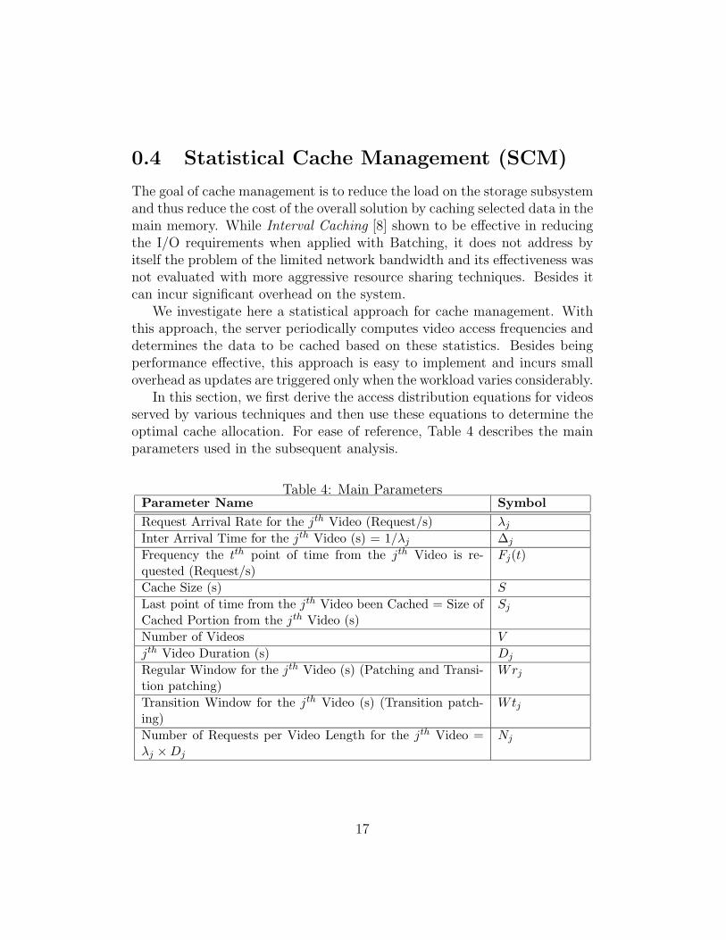
In this section, we first derive the access distribution equations for videosserved by various techniques and then use these equations to determine theoptimal cache allocation. For ease of reference, Table 4 describes the mainparameters used in the subsequent analysis.

Table 4: Main ParametersParameter Name SymbolRequest Arrival Rate for the jth Video (Request/s) λj

Inter Arrival Time for the jth Video (s) = 1/λj Δj

Frequency the tth point of time from the jth Video is re-quested (Request/s)

Fj(t)

Cache Size (s) S

Last point of time from the jth Video been Cached = Size ofCached Portion from the jth Video (s)

Sj

Number of Videos V

jth Video Duration (s) Dj

Regular Window for the jth Video (s) (Patching and Transi-tion patching)

Wrj

Transition Window for the jth Video (s) (Transition patch-ing)

Wtj

Number of Requests per Video Length for the jth Video =λj × Dj

Nj

17

0.4.1 Video Access Distributions

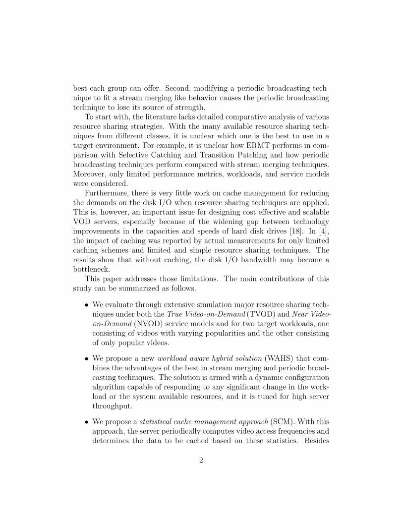
We derive next the access distribution equations for each playback point ina video delivered using various techniques. We assume here a TVOD modelwhere every request is served immediately (except for Periodic Broadcasting).Hence, the average service rate of video j is the same as its average requestarrival rate (λj). We also assume that Fj(t) is the rate (frequency) by whichthe tth point of time of video j is requested from the disks when there is nocache. The derived equations were validated by simulation. In Figures 3(a)through 3(d) we report the results for a video with a request arrival rate of2 requests per minute (which is the rate for the second most popular videoin the mixed workload, discussed in Section 0.6).

Patching and Controlled Multicast

Because of having two types of streams in Patching (and Controlled Mul-ticast), and having a limit on the maximum patch length (Wrj), the videocan be divided into two regions: [0,Wrj] and [Wrj, Dj]. Since every regu-lar stream delivers the full video data, all points in the second region willbe requested with an equal rate: 1/Wrj. The situation is different for thefirst region because the patches vary in length. The closer the point to thebeginning of the video, the more likely it will be missed and requested bypatches. The access rate approaches the video request rate (λj) as the pointbecomes closer to the beginning. Consequently, the access distribution canbe formulated as follows:

Fj(t)=

8>><>>:

λj − (λj

Wrj− 1

(Wrj)2)t 0 ≤ t < Wrj,

1Wrj

Wrj ≤ t ≤ Dj.(14)

Figure 3(a) shows that the analytical and simulation results match almostperfectly.

Transition Patching

Transition Patching has three types of streams: patches with maximumlength of Wtj, transition patches with lengths between 3Wtj and Wrj +2Wtj, and the regular streams with full video length. Therefore, the region[Wrj + 2Wtj, Dj] is delivered by only regular streams at an access rate of1/Wrj. As in Patching, the rate for region [0,Wtj] decreases linearly from λj

18

to 1/Wtj. The region [Wtj, 3Wtj] is delivered by every transition patch andregular stream, and thus the rate is 1/Wtj. The region [3Wtj, 4Wtj] is deliv-ered by every transition patch and regular stream except the first transitionpatch in every regular window (Wrj). The region [4Wtj, 5Wtj] is deliveredby every transition patch and regular stream except the first two transitionpatches in every regular window. The pattern continues up to the region[Wrj +Wtj,Wrj +2Wtj], which is delivered by only regular streams and thelast transition patch in every regular window, leading to a stair shape curve.Consequently, the access distribution can be formulated as follows:

Fj(t)=

8>>>>>>>>><>>>>>>>>>:

λj − (λj

Wtj− 1

(Wtj)2)t 0 ≤ t < Wtj,

1Wtj

Wtj ≤ t < 3Wtj,1

Wtj− n

Wrj3Wtj ≤ t < Wrj + 2Wtj,

1Wrj

Wrj + 2Wtj ≤ t ≤ Dj,

(15)

where n = � tWtj

� − 2. Equation (15) was validated by simulation and the

error is very small, as shown in Figure 3(b).

ERMT

Let us reexamine Figure 1(c) and assume that the inter-arrival time betweensuccessive requests for video j is Δj. (In reality, a customer does not arriveevery exactly Δj, but this will be the average behavior over a long period.)Thus, 4 out of the 8 streams (fraction = 1

2) have length 1 × Δj, 2 streams

(fraction = 14) have length 4×Δj, and 1 stream (fraction = 1

8) have length

10 × Δj on the average. This pattern can be generalized as follows: for

Nj requests per video length,Nj

16streams of the Nj streams are with length

22 × Δj,Nj

32with length 46 × Δj,

Nj

2i with length L(i) × Δj, and so on tilli = log2(Nj), where L(i) = 2×L(i− 1) + 2, and L(1) = Δj. Hence, the firstpart of the video from the beginning to Δj is delivered (i.e. requested) byevery stream, with a request frequency equal to λj. The second part from Δj

to 4×Δj is requested by Nj −Nj/2 streams. The third part from 4×Δj to10×Δj is requested by Nj −Nj/2−Nj/4 streams, and so on. To generalize,the access frequency for the tth point of time in the jth video is given by

Fj(t) =λj

2(1+�log2 (t/Δj+2)/3�) . (16)

19

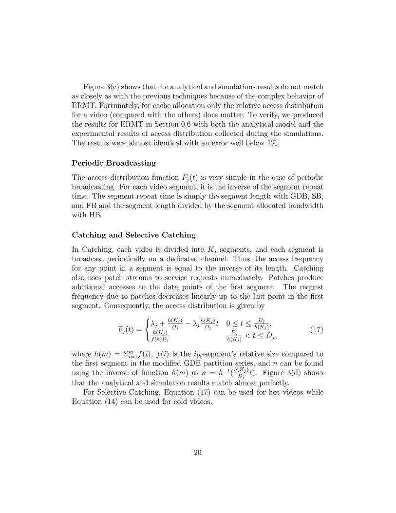
Figure 3(c) shows that the analytical and simulations results do not matchas closely as with the previous techniques because of the complex behavior ofERMT. Fortunately, for cache allocation only the relative access distributionfor a video (compared with the others) does matter. To verify, we producedthe results for ERMT in Section 0.6 with both the analytical model and theexperimental results of access distribution collected during the simulations.The results were almost identical with an error well below 1%.

Periodic Broadcasting

The access distribution function Fj(t) is very simple in the case of periodicbroadcasting. For each video segment, it is the inverse of the segment repeattime. The segment repeat time is simply the segment length with GDB, SB,and FB and the segment length divided by the segment allocated bandwidthwith HB.

Catching and Selective Catching

In Catching, each video is divided into Kj segments, and each segment isbroadcast periodically on a dedicated channel. Thus, the access frequencyfor any point in a segment is equal to the inverse of its length. Catchingalso uses patch streams to service requests immediately. Patches produceadditional accesses to the data points of the first segment. The requestfrequency due to patches decreases linearly up to the last point in the firstsegment. Consequently, the access distribution is given by

Fj(t) =

{λj +

h(Kj)

Dj− λj

h(Kj)

Djt 0 ≤ t ≤ Dj

h(Kj),

h(Kj)

f(n)Dj

Dj

h(Kj)< t ≤ Dj,

(17)

where h(m) = Σmi=1f(i), f(i) is the ith-segment’s relative size compared to

the first segment in the modified GDB partition series, and n can be foundusing the inverse of function h(m) as n = h−1(

h(Kj)

Djt). Figure 3(d) shows

that the analytical and simulation results match almost perfectly.For Selective Catching, Equation (17) can be used for hot videos while

Equation (14) can be used for cold videos.

20

WAHS

For WAHS, Equation (16) can be used for the ERMT videos, while thecalculations discussed in Subsection (0.4.1) applies for Fibonacci videos.

0.4.2 Cache Allocation Model

The derived access distribution models in the previous subsection exhibit thefollowing property: Fj(t1) ≥ Fj(t2) for all t1 < t2. If the optimal cached sizefor the jth video is found to be Sj seconds, then we simply cache from thebeginning of the video till the Sj

th second. To allocate the available cacheoptimally among all videos under such property, we simply need to solve twoequations:

S =V∑

j=1

Sj, (18)

andFi(Si) = Fj(Sj), (19)

for all i, j ∈ V ideosSet with Si and Sj > 0. Equation (19) means that for allvideos with cached portions greater than zero, the request frequency of thelast cached frame for every video must be equal (or very close).

657 2000 3000 4000 5000 6000 72000

0.2

0.4

0.6

0.8

1

1.2

1.4

1.6

1.8

2

Point of Time in the Video (second)

Req

ues

t / M

inu

te

Patching − Analytical Patching − Simulation

(a) Patching

240 1000 2000 3000 4000 5000 6000 72000

0.2

0.4

0.6

0.8

1

1.2

1.4

1.6

1.8

2


Req

ues

t / M

inu

te

Transition Patching − Analytical Transition Patching − Simulation

(b) TransitionPatching

1000 2000 3000 4000 5000 6000 72000

0.5

1

1.5

2

2.5


Req

ues

t / M

inu

te

ERMT − Analytical ERMT − Simulation

(c) ERMT

1000 2000 3000 4000 5000 6000 72000

0.5

1

1.5

2

2.5


Req

ues

t / M

inu

te

Catching − Analytical Catching − Simulation

(d) Catching

Figure 3: Access Distribution Fj(t)

0.5 Tunings of Design Parameters

In this section, we derive equations for determining optimally the valuesof Wr and Wt for Transition Patching. For Selective Catching, we presentan approach for deciding on what videos to serve with Catching and what

21

videos with Controlled Multicast when the server resources are limited. Noapproach was provided in [16] for such situations. For the other techniques,we highlight important results reported in [19, 16, 15].

0.5.1 Transition Patching

The objective here is to derive simple equations for Wr and Wt, whichminimize the number of required server channels. The number of requiredchannels (chj) with any technique is given by

chj =

∫ Dj

0

Fj(t)dt, (20)

where Fj(t) is the request distribution for the chosen technique. For Transi-tion Patching,

chj =1

2λjWtj +

1

2

Wrj

Wtj+

Dj

Wrj

− 2WtjWrj

+ 1. (21)

By taking the first derivative of Equation (21) with respect to Wrj andequating it with zero, we get the optimal value of Wrj:

Wrj =√

2Wtj(Dj − 2Wtj). (22)

Since the transition patch cannot exceed the video length (i.e., Wrj +2Wtj <Dj) and Wtj < Wrj, it follows that Wtj < 1

3Dj.

Similarly, to find the optimal value of Wtj, we take the first derivativeof Equation (21) with respect to Wtj and equate it with zero, and thensubstitute the value of Wrj from Equation (22):

Wtj = 3

√2DjΔ2

j/3

√1 − 2Wtj/Dj. (23)

Typically, Dj >> 2Wtj, and thus

Wtj ≈ 3

√2Dj/λ2

j = 3

√2Δ2

jDj. (24)

Alternatively, we can substitute this value in Equation (23) and get thefollowing equation that is more accurate:

Wtj ≈ 3

√2Δ2

jDj/3

√1 − 2 3

√2Δ2

j/D2j . (25)

22

To avoid a negative value of Wtj, Nj = λjDj > 4. (It can be shown that forTransition Patching to be more cost effective than Patching, Nj = λjDj ≥12.) By optimizing the number of channels Equation (21) with respect toWrj and Wtj, and assuming Wtj << Dj, we obtain:

Wrjopt =√

2Wtj(Dj − 2Wtj)

and

Wtjopt ≈ 3

√2Δ2

jDj/3

√1 − 2 3

√2Δ2

j/D2j .

Note that for Transition Patching to be more cost effective than Patching,Nj = λjDj ≥ 12.

0.5.2 Patching and Controlled Multicast

In [19], an optimal value for Wrj in Patching/Controlled Multicast was de-rived:

Wrj =√

2Dj/λj =√

2ΔjDj. (26)

Based on that, the number of required channels can be given by

chj =√

2λjDj − 1/2. (27)

A slightly different equation was reached in [15], but our analysis favorsEquation (26). Equations (27) and (26) assume Nj = λjDj > 1; otherwise,no two streams will overlap and a unicast is the only option.

0.5.3 Catching and Selective Catching

In [15] and [16], the optimal number of server channels required for ControlledMulticast/Patching and for Catching were shown to be

chj =√

2λjDj + 1 − 1 (28)

andchj = K∗

j + λjFSj/2, (29)

respectively. Where FSj is the first segment length of video j and K∗j is the

optimal number of broadcast channels. This equation can be optimized withrespect to Kj to find the optimal value K∗

j . In Selective Catching, a key issue

23

is how to decide whether a video is hot or cold. One possible approach is tocompare the numbers of required channels to serve the video with Catchingand with Controlled Multicast [16]. The video is considered hot if the firstnumber is smaller and cold otherwise. By comparing the required channelsby both, the technique that results in smaller value is chosen for service[16]. Unfortunately, in many situations the number of server channels is notsufficient to satisfy the Catching requirement for every hot video. In that casewe need to determine the subset of the hot videos to be served by Catching.We introduce the following additional test: video j is served by Catching if

ServerChannels × λj

λ≥ chj. (30)

The idea here is to serve by Catching, among the hot videos, only the videoswhose numbers of required channels are not greater than their fair share,determined by their contributions to the total number of requests.

0.6 Performance Evaluation

0.6.1 Evaluation Methodology

We have developed a simulator for VOD that models various resource sharingtechniques and captures the derived analytical models for cache management.The simulator has been validated by reproducing graphs in previous studies.Simulation stop after a steady state analysis with 95% confidence interval isreached.

We consider two service models: True Video-on-Demand (TVOD) andNear Video-on-Demand (NVOD). We also consider two video workloads:mixed-video and hot-video. The mixed-video workload contains videos withpopularities varying from cold to hot, and the hot-video workload containsonly hot videos. The later is used mainly to evaluate periodic broadcastingtechniques which are designed mainly for popular videos. The two servicemodels and the two video workloads lead to four target environments: mixed-video workload and TVOD, hot-video workload and TVOD, mixed-video work-load and NVOD, and hot-video workload and NVOD.

In the TVOD model, we compare the server resources required to ser-vice all requests immediately. In the NVOD model, however, we fix theserver resources and compare the customer defection probability (defined as

24

the probability that customers leave the server without being serviced be-cause of waiting times exceeding their tolerance), the average waiting time,and unfairness towards cold videos. The first metric translates directly tothe number of customers that can be serviced concurrently and to serverthroughput. Two types of server resources are considered: server channelsand disk channels. Server channels represent the requirement in networkbandwidth, whereas disk channels represent the disk I/O bandwidth require-ment. A channel is capable of supporting only one stream at a time. Withoutcache in the main memory to reduce the load on the storage subsystem, thenumber of disk channels is equal to the number of server channels.

0.6.2 Workload Characteristics

In accordance with most prior studies, we assume that the arrival of requestsfollows a Poisson Process with an average arrival rate λ and that the accessesto videos are highly localized and follow a Zipf-like distribution with skewnessparameter θ = 0.271. The mixed-video workload contains 120 2-hour videos,whereas in the hot-video workload we consider three numbers of videos: 1,10, and 20 2-hour each. Table 5 shows the values of the input parameters inboth workloads.

We consider two models of customer waiting tolerance. In general, weassume as in prior work that the tolerance follows the exponential distributionwith a mean value of 2 minutes. While with periodic broadcasting techniques,we borrow and apply the Time of Service Guarantee (TSG) model [31, 34],which was used in a different context, since broadcasting techniques canprovide time of service guarantees by upper limiting the waiting times bythe length of the first segment. With TSG, customers who receive time ofservice guarantees shorter than 2 minutes will wait to be serviced, whereas thewaiting tolerance of all other customers follows the exponential distributionwith a mean value of 2 minutes.

For scheduling, we use Maximum Queue Length (MQL) [10] and FirstCome First Serve (FCFS) [10]. The results for Maximum Factored QueueLength (MFQL) [1] are not shown because it performs poorly in the streamingmerging environment (despite its relatively good performance with Batch-ing).

25

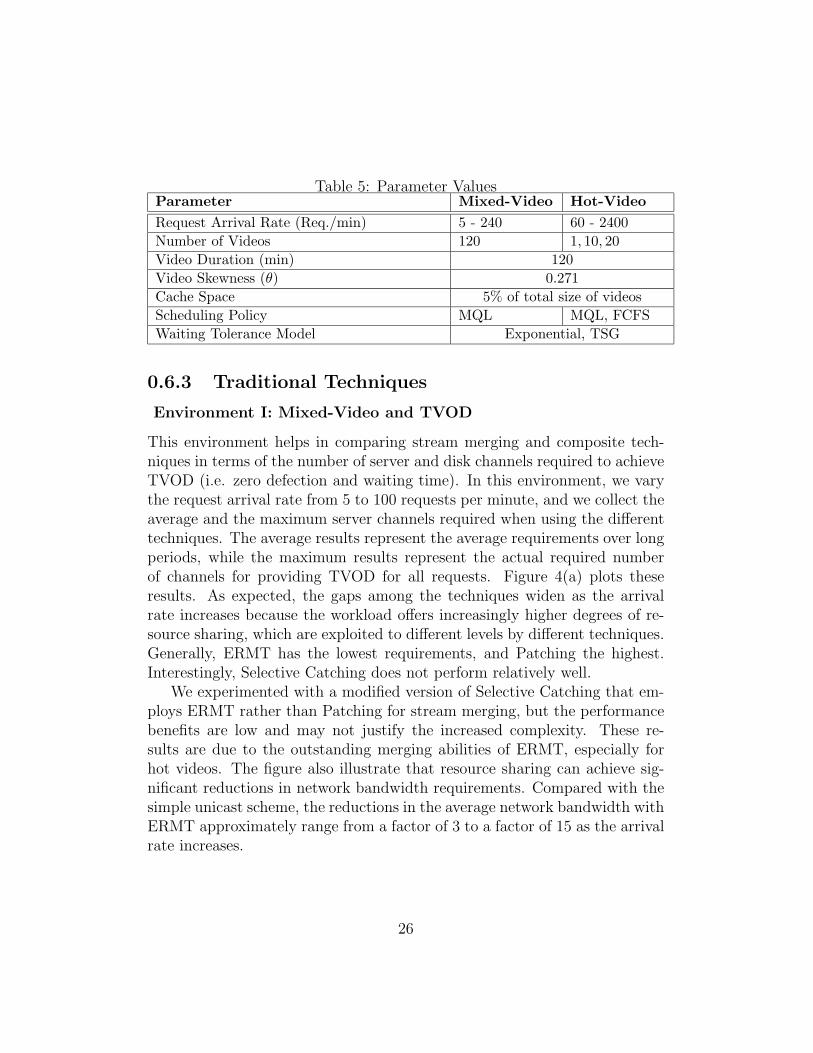
Table 5: Parameter ValuesParameter Mixed-Video Hot-VideoRequest Arrival Rate (Req./min) 5 - 240 60 - 2400Number of Videos 120 1, 10, 20Video Duration (min) 120Video Skewness (θ) 0.271Cache Space 5% of total size of videosScheduling Policy MQL MQL, FCFSWaiting Tolerance Model Exponential, TSG

0.6.3 Traditional Techniques

Environment I: Mixed-Video and TVOD

This environment helps in comparing stream merging and composite tech-niques in terms of the number of server and disk channels required to achieveTVOD (i.e. zero defection and waiting time). In this environment, we varythe request arrival rate from 5 to 100 requests per minute, and we collect theaverage and the maximum server channels required when using the differenttechniques. The average results represent the average requirements over longperiods, while the maximum results represent the actual required numberof channels for providing TVOD for all requests. Figure 4(a) plots theseresults. As expected, the gaps among the techniques widen as the arrivalrate increases because the workload offers increasingly higher degrees of re-source sharing, which are exploited to different levels by different techniques.Generally, ERMT has the lowest requirements, and Patching the highest.Interestingly, Selective Catching does not perform relatively well.

We experimented with a modified version of Selective Catching that em-ploys ERMT rather than Patching for stream merging, but the performancebenefits are low and may not justify the increased complexity. These re-sults are due to the outstanding merging abilities of ERMT, especially forhot videos. The figure also illustrate that resource sharing can achieve sig-nificant reductions in network bandwidth requirements. Compared with thesimple unicast scheme, the reductions in the average network bandwidth withERMT approximately range from a factor of 3 to a factor of 15 as the arrivalrate increases.

26

10 20 30 40 50 60 70 80 90 1000

500

1000

1500

2000

Request Rate (requests/minute)

R

equ

ired

Ser

ver

Ch

ann

els

Per

Vid

eo

Average ERMT

Patching

Selective Catching

Transition Patching

10 20 30 40 50 60 70 80 90 1000

500

1000

1500

2000


Actual (Maximum)

(a) Effect of Request Rate onRequired Channels

Figure 4: Environment I

200 400 600 800 1000 1200 1400 1600 1800 2000 2200 24005

10

15

20

25


Req

uir

ed S

erve

r C

han

nel

s P

er V

ideo

Average

ERMT (1 video) ERMT (10 videos) ERMT (20 videos)

200 400 600 800 1000 1200 1400 1600 1800 2000 2200 2400

10

15

20

25

30

35

40


Actual (Maximum)

SBGDBFB

SBGDBFB

(a) Effect of Request Rate onRequired Channels

20 60 120 2400

5

10

15


Average ERMT (1 video)

ERMT (10 videos, MQL)

ERMT (10 videos, FCFS)

ERMT (20 videos, MQL)

ERMT (20 videos, FCFS)

20 60 120 2400

100

200

300

400

C

ust

om

er W

aiti

ng

Tim

e (s

eco

nd

)

Maximum


(b) Effect of Request Rate onWaiting Time (Average Re-quired Channels Provided)

Figure 5: Environment II

Environment II: Hot-Video and TVOD

In this environment, we compare the performance of various periodic broad-casting techniques (SB, GDB, and FB) and the best performer in Environ-ment I (ERMT). Since periodic broadcasting cannot provide a zero waitingtime, we assume that a maximum waiting time below 2 seconds constitutesa TVOD service.

Figure 5(a) plots the average and maximum required server channels pervideo to provide TVOD for the different techniques. Note that unlike periodicbroadcasting, the number of server channels per video with ERMT dependson the arrival rate and the number of supported videos. Whereas periodicbroadcasting techniques reserve channels for each video, ERMT deals with allthe resources as one pool and distributes them dynamically to the requests.While the average helps in understanding the overall system load, the maxi-mum indicates the actual bandwidth to be reserved to achieve TVOD. Thedistinction between the two metrics was always ignored in previous studies,where only the average results were usually reported. The results demon-strate that ERMT scales very well with the increase in request rate even interms of both the average and actual (maximum) required bandwidth. Fora workload of 20 2-hour videos, the request rate must be constantly over900 requests/minute for the best periodic broadcasting technique (FB) tobe a better choice than ERMT. Even when that is the case, while ERMTrequires more guaranteed bandwidth, it does not consume it all the time,which may enable the system to face short periods of drops in server capac-ity. Since the required bandwidth with ERMT is a function of the number

27

of requests per video length (i.e., N = λD), the breakpoint is higher than900 requests/minute when the videos are shorter.

To highlight the effect of the difference between the average and actualrequired number of channels, Figure 5(b) plots the average and maximumcustomer waiting times if only the average required bandwidth is provided.Therefore, the number of provided channels varies with the request rate andwith the number of videos as well. The service is obviously not TVOD, espe-cially for the relatively low request rates since some customers had to wait fewminutes for service. Since scheduling policies can impact the performance ofERMT compared with periodic broadcasting, both MQL and FCFS are ex-amined. MQL achieves higher throughput and shorter average waiting time,whereas FCFS is fairer and can significantly reduce the maximum waitingtime.

Environment III: Mixed-Video and NVOD

By varying the number of server channels, we can use this environment tocompare stream merging and composite techniques in terms of the achievedaverage customer defection probability, waiting times, and unfairness. Figure6 plots these three metrics versus the number of server channels for varioustechniques. The results here demonstrate once again that ERMT performsthe best and Patching the worst among stream merging and composite tech-niques. There is a clear correlation among the three metrics. The correla-tion between unfairness and the other two metrics is due to using MaximumQueue Length (MQL) [10] for scheduling. MQL selects for service the longestvideo queue, trading fairness for performance. The more limited the numberof channels becomes, the longer customers have to wait, and the faster thewaiting queues build up. Consequently, both the defection probability andthe bias against cold videos increase.

Environment IV: Hot-Video and NVOD

In this environment, we also compare the performance of various periodicbroadcasting techniques with ERMT. We consider here two waiting toler-ance models: exponential and TSG (discussed in Subsection 0.6.2). Thelater captures the capability of periodic broadcasting techniques to limit themaximum waiting time and predict the actual times of service. By informingclients upon arrival with their times of service, the server can encourage them

28

300 350 400 450 500 550 600 650 7000

10

20

30

40

50

60


Cu

sto

mer

Def

ecti

on

Per

cen

tag

e

ERMT Patching Selective Catching Transition Patching

(a) Effect of Server Channelson Defection Probability

300 350 400 450 500 550 600 650 7000

5

10

15

20

25

30

35

40

45

50


Ave

rag

e C

ust

om

er W

aiti

ng

Tim

e (s

eco

nd

) ERMT Patching Selective Catching Transition Patching

(b) Effect of Server Channelson Average Waiting Time

300 350 400 450 500 550 600 650 7000

0.002

0.004

0.006

0.008

0.01

0.012

0.014


Un

fair

nes

s


(c) Effect of Server Channelson Unfairness

Figure 6: Environment III [30 Requests/Minute]

to wait.Figures 7(a) through 7(d) depict the defection probability and average

waiting time under the exponential waiting tolerance model for differentserver capacities, request rates, and numbers of videos. These results con-firm that ERMT is very competitive, compared with the best periodic broad-casting technique, even in servicing very hot videos and under very limitedresources.

Figures 7(e) and 7(f) compare various techniques in terms of the defectionprobability and average waiting time under the TSG waiting tolerance model,which captures the ability of the broadcasting techniques in providing waitingtime guarantees. The results demonstrate that broadcasting techniques canachieve much lower defection probabilities than ERMT, especially when theavailable server bandwidth is not very limited. With only 8 server channelsper video, all broadcasting techniques cause no defections, whereas ERMTcauses more than 20% defections. However, ERMT achieves shorter averagewaiting time for those clients who were serviced, partially due to the highdefection percentage.

Cautious Harmonic Broadcasting (CHB)

Despite its high effectiveness in reducing server bandwidth, Cautious Har-monic Broadcasting (CHB) requires high client bandwidth. The requirednumber of client channels is equal to the number server channels allocatedfor the video. In contrast, FB, SB, GDB, and ERMT always require onlytwo channels. Moreover, CHB partitions each supported video into a largenumber of segments. For example, to achieve a maximum waiting time of

29

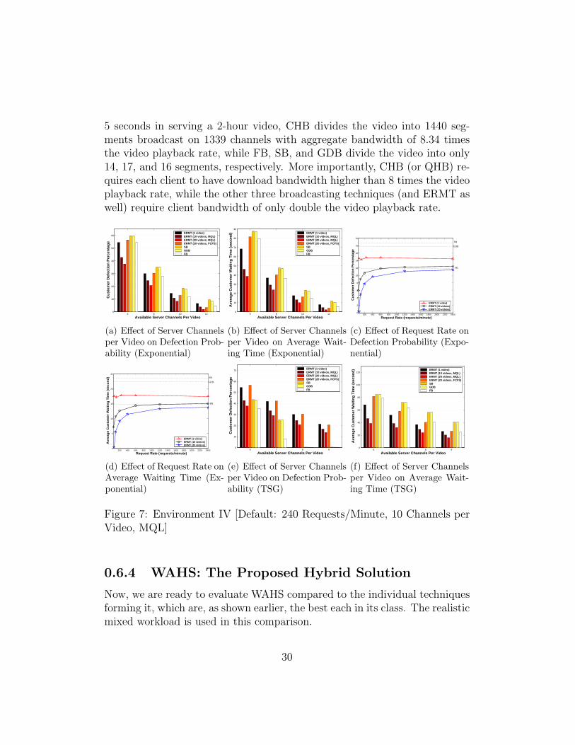
5 seconds in serving a 2-hour video, CHB divides the video into 1440 seg-ments broadcast on 1339 channels with aggregate bandwidth of 8.34 timesthe video playback rate, while FB, SB, and GDB divide the video into only14, 17, and 16 segments, respectively. More importantly, CHB (or QHB) re-quires each client to have download bandwidth higher than 8 times the videoplayback rate, while the other three broadcasting techniques (and ERMT aswell) require client bandwidth of only double the video playback rate.

6 8 10 120

10

20

30

40

50

60


Cu

sto

mer

Def

ecti

on

Per

cen

tag

e

ERMT (1 video) ERMT (10 videos, MQL) ERMT (20 videos, MQL) ERMT (20 videos, FCFS) SB GDB FB

(a) Effect of Server Channelsper Video on Defection Prob-ability (Exponential)

6 8 10 120

10

20

30

40

50

60

70

80

90


Ave

rag

e C

ust

om

er W

aiti

ng

Tim

e (s

eco

nd

) ERMT (1 video) ERMT (10 videos, MQL) ERMT (20 videos, MQL) ERMT (20 videos, FCFS) SB GDB FB

(b) Effect of Server Channelsper Video on Average Wait-ing Time (Exponential)

200 400 600 800 1000 1200 1400 1600 1800 2000 2200 24000

2

4

6

8

10

12

14

16

18

20


Cu

sto

mer

Def

ecti

on

Per

cen

tag

e


SB

GDB

FB

(c) Effect of Request Rate onDefection Probability (Expo-nential)

200 400 600 800 1000 1200 1400 1600 1800 2000 2200 24000

5

10

15

20

25


Ave

rag

e C

ust

om

er W

aiti

ng

Tim

e (s

eco

nd

)


SB

GDB

FB

(d) Effect of Request Rate onAverage Waiting Time (Ex-ponential)

6 7 8 90

10

20

30

40

50

60

70


Cu

sto

mer

Def

ecti

on

Per

cen

tag

e

ERMT (1 video) ERMT (10 videos, MQL) ERMT (20 videos, MQL) ERMT (20 videos, FCFS) SB GDB FB

(e) Effect of Server Channelsper Video on Defection Prob-ability (TSG)

6 7 8 90

20

40

60

80

100

120


Ave

rag

e C

ust

om

er W

aiti

ng

Tim

e (s

eco

nd

) ERMT (1 video) ERMT (10 videos, MQL) ERMT (20 videos, MQL) ERMT (20 videos, FCFS) SB GDB FB

(f) Effect of Server Channelsper Video on Average Wait-ing Time (TSG)

Figure 7: Environment IV [Default: 240 Requests/Minute, 10 Channels perVideo, MQL]

0.6.4 WAHS: The Proposed Hybrid Solution

Now, we are ready to evaluate WAHS compared to the individual techniquesforming it, which are, as shown earlier, the best each in its class. The realisticmixed workload is used in this comparison.

30

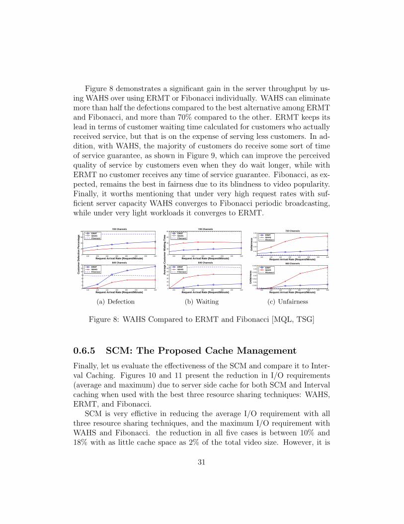
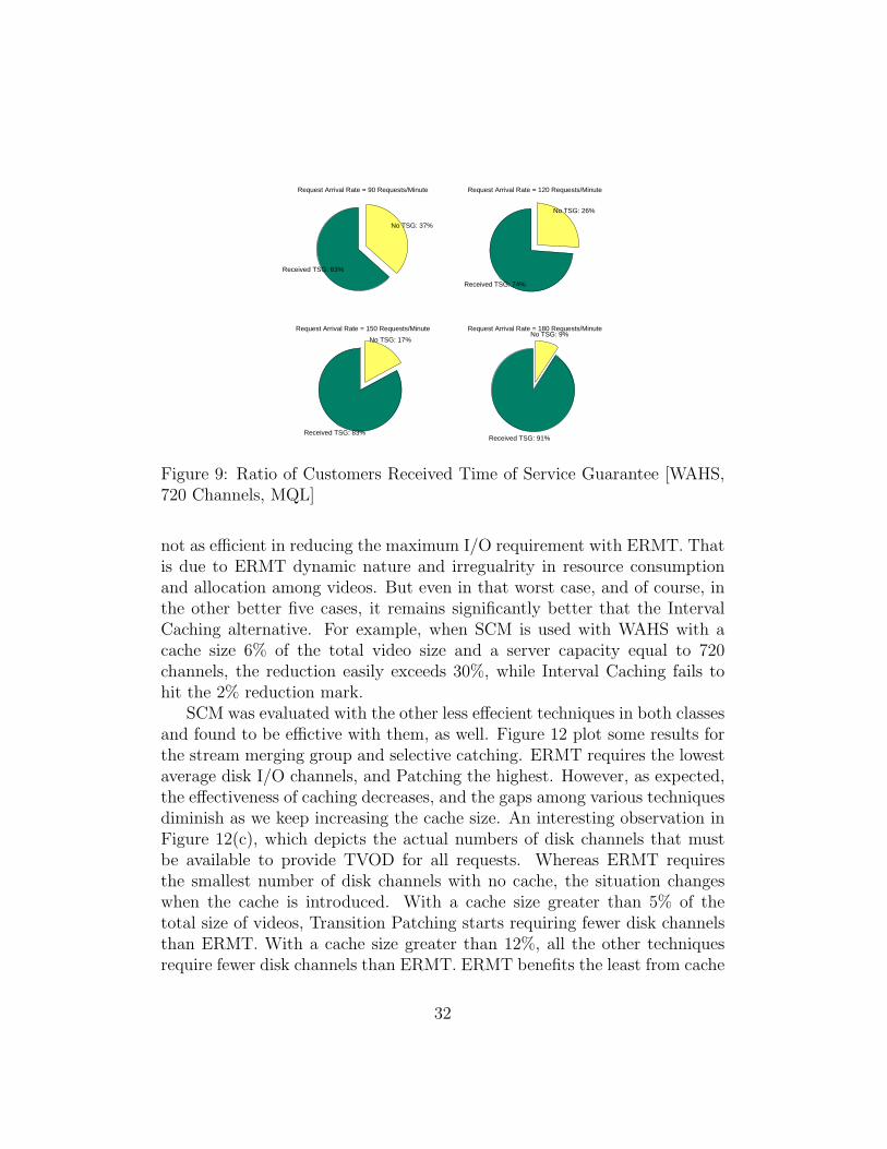
Figure 8 demonstrates a significant gain in the server throughput by us-ing WAHS over using ERMT or Fibonacci individually. WAHS can eliminatemore than half the defections compared to the best alternative among ERMTand Fibonacci, and more than 70% compared to the other. ERMT keeps itslead in terms of customer waiting time calculated for customers who actuallyreceived service, but that is on the expense of serving less customers. In ad-dition, with WAHS, the majority of customers do receive some sort of timeof service guarantee, as shown in Figure 9, which can improve the perceivedquality of service by customers even when they do wait longer, while withERMT no customer receives any time of service guarantee. Fibonacci, as ex-pected, remains the best in fairness due to its blindness to video popularity.Finally, it worths mentioning that under very high request rates with suf-ficient server capacity WAHS converges to Fibonacci periodic broadcasting,while under very light workloads it converges to ERMT.

100 120 140 160 180 200 220 2400

10

20

30

40

Cu

sto

mer

Def

ecti

on

Per

cen

tag

e


720 Channels

ERMT WAHS Fibonacci

100 120 140 160 180 200 220 2400

2

4

6

8

10

12

14


840 Channels

ERMT WAHS Fibonacci

(a) Defection

100 120 140 160 180 200 220 2400

20

40

60

80

Ave

rag

e C

ust

om

er W

aiti

ng

Tim

e


720 Channels

ERMT WAHS Fibonacci

100 120 140 160 180 200 220 2400

10

20

30

40

50

60

70


840 Channels

ERMT WAHS Fibonacci

(b) Waiting

100 120 140 160 180 200 220 2400

0.01

0.02

0.03

0.04

0.05

Un

fair

nes

s


720 Channels

ERMT WAHS Fibonacci

100 120 140 160 180 200 220 2400

0.005

0.01

0.015

0.02

0.025

0.03

0.035

Un

fair

nes

s


840 Channels

ERMT WAHS Fibonacci

(c) Unfairness

Figure 8: WAHS Compared to ERMT and Fibonacci [MQL, TSG]

0.6.5 SCM: The Proposed Cache Management

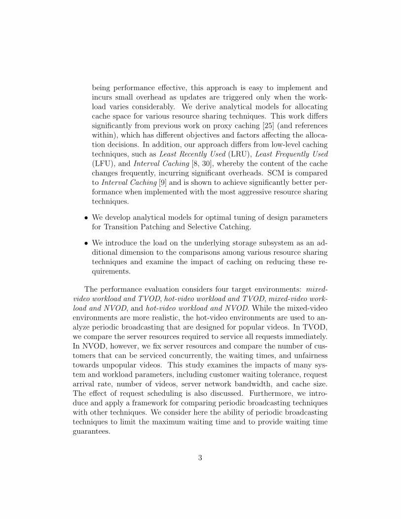
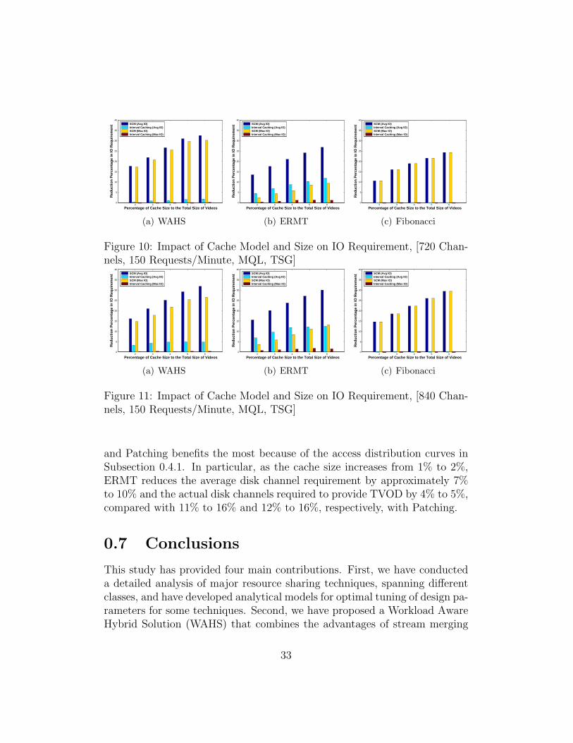
Finally, let us evaluate the effectiveness of the SCM and compare it to Inter-val Caching. Figures 10 and 11 present the reduction in I/O requirements(average and maximum) due to server side cache for both SCM and Intervalcaching when used with the best three resource sharing techniques: WAHS,ERMT, and Fibonacci.

SCM is very effictive in reducing the average I/O requirement with allthree resource sharing techniques, and the maximum I/O requirement withWAHS and Fibonacci. the reduction in all five cases is between 10% and18% with as little cache space as 2% of the total video size. However, it is

31

Received TSG: 63%

No TSG: 37%

Request Arrival Rate = 90 Requests/Minute

Received TSG: 74%

No TSG: 26%


Received TSG: 83%

No TSG: 17%


Received TSG: 91%

No TSG: 9%Request Arrival Rate = 180 Requests/Minute

Figure 9: Ratio of Customers Received Time of Service Guarantee [WAHS,720 Channels, MQL]

not as efficient in reducing the maximum I/O requirement with ERMT. Thatis due to ERMT dynamic nature and irregualrity in resource consumptionand allocation among videos. But even in that worst case, and of course, inthe other better five cases, it remains significantly better that the IntervalCaching alternative. For example, when SCM is used with WAHS with acache size 6% of the total video size and a server capacity equal to 720channels, the reduction easily exceeds 30%, while Interval Caching fails tohit the 2% reduction mark.

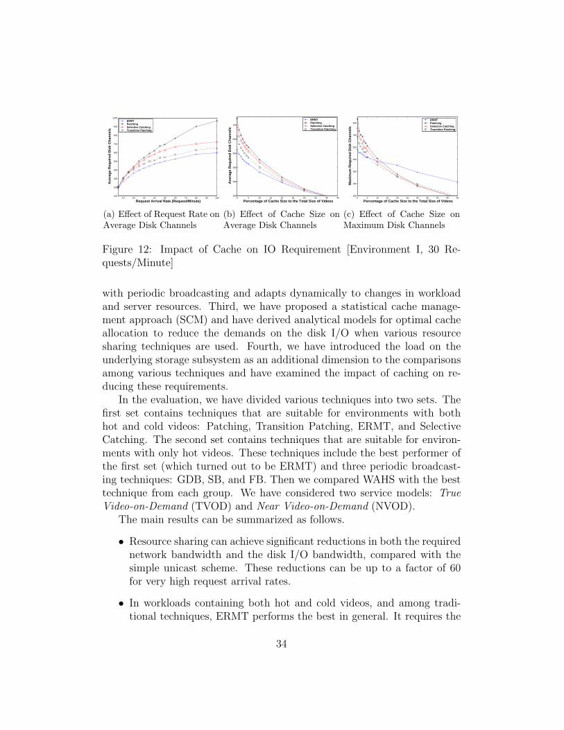
SCM was evaluated with the other less effecient techniques in both classesand found to be effictive with them, as well. Figure 12 plot some results forthe stream merging group and selective catching. ERMT requires the lowestaverage disk I/O channels, and Patching the highest. However, as expected,the effectiveness of caching decreases, and the gaps among various techniquesdiminish as we keep increasing the cache size. An interesting observation inFigure 12(c), which depicts the actual numbers of disk channels that mustbe available to provide TVOD for all requests. Whereas ERMT requiresthe smallest number of disk channels with no cache, the situation changeswhen the cache is introduced. With a cache size greater than 5% of thetotal size of videos, Transition Patching starts requiring fewer disk channelsthan ERMT. With a cache size greater than 12%, all the other techniquesrequire fewer disk channels than ERMT. ERMT benefits the least from cache

32

2 3 4 5 60

5

10

15

20

25

30

35

40

Red

uct

ion

Per

cen

tag

e in

IO R

equ

irem

ent

Percentage of Cache Size to the Total Size of Videos

SCM (Avg IO) Interval Caching (Avg IO) SCM (Max IO) Interval Caching (Max IO)

(a) WAHS

2 3 4 5 60

5

10

15

20

25

30

35

40

Red

uct

ion

Per

cen

tag

e in

IO R

equ

irem

ent



(b) ERMT

2 3 4 5 60

5

10

15

20

25

30

35

40

Red

uct

ion

Per

cen

tag

e in

IO R

equ

irem

ent



(c) Fibonacci

Figure 10: Impact of Cache Model and Size on IO Requirement, [720 Chan-nels, 150 Requests/Minute, MQL, TSG]

2 3 4 5 60

5

10

15

20

25

30

35

40

Red

uct

ion

Per

cen

tag

e in

IO R

equ

irem

ent



(a) WAHS

2 3 4 5 60

5

10

15

20

25

30

35

40

Red

uct

ion

Per

cen

tag

e in

IO R

equ

irem

ent



(b) ERMT

2 3 4 5 60

5

10

15

20

25

30

35

40

Red

uct

ion

Per

cen

tag

e in

IO R

equ

irem

ent



(c) Fibonacci

Figure 11: Impact of Cache Model and Size on IO Requirement, [840 Chan-nels, 150 Requests/Minute, MQL, TSG]

and Patching benefits the most because of the access distribution curves inSubsection 0.4.1. In particular, as the cache size increases from 1% to 2%,ERMT reduces the average disk channel requirement by approximately 7%to 10% and the actual disk channels required to provide TVOD by 4% to 5%,compared with 11% to 16% and 12% to 16%, respectively, with Patching.

0.7 Conclusions

This study has provided four main contributions. First, we have conducteda detailed analysis of major resource sharing techniques, spanning differentclasses, and have developed analytical models for optimal tuning of design pa-rameters for some techniques. Second, we have proposed a Workload AwareHybrid Solution (WAHS) that combines the advantages of stream merging

33

10 20 30 40 50 60 70 80 90 100100

200

300

400

500

600

700

800

900

1000


Ave

rag

e R

equ

ired

Dis

k C

han

nel

s


(a) Effect of Request Rate onAverage Disk Channels

0 5 10 15 20 25 30 35 40 45200

300

400

500

600

700


Ave

rag

e R

equ

ired

Dis

k C

han

nel

s


(b) Effect of Cache Size onAverage Disk Channels

0 5 10 15 20 25 30 35 40 45 50200

300

400

500

600

700

800


Max

imu

m R

equ

ired

Dis

k C

han

nel

s


(c) Effect of Cache Size onMaximum Disk Channels

Figure 12: Impact of Cache on IO Requirement [Environment I, 30 Re-quests/Minute]

with periodic broadcasting and adapts dynamically to changes in workloadand server resources. Third, we have proposed a statistical cache manage-ment approach (SCM) and have derived analytical models for optimal cacheallocation to reduce the demands on the disk I/O when various resourcesharing techniques are used. Fourth, we have introduced the load on theunderlying storage subsystem as an additional dimension to the comparisonsamong various techniques and have examined the impact of caching on re-ducing these requirements.

In the evaluation, we have divided various techniques into two sets. Thefirst set contains techniques that are suitable for environments with bothhot and cold videos: Patching, Transition Patching, ERMT, and SelectiveCatching. The second set contains techniques that are suitable for environ-ments with only hot videos. These techniques include the best performer ofthe first set (which turned out to be ERMT) and three periodic broadcast-ing techniques: GDB, SB, and FB. Then we compared WAHS with the besttechnique from each group. We have considered two service models: TrueVideo-on-Demand (TVOD) and Near Video-on-Demand (NVOD).

The main results can be summarized as follows.

• Resource sharing can achieve significant reductions in both the requirednetwork bandwidth and the disk I/O bandwidth, compared with thesimple unicast scheme. These reductions can be up to a factor of 60for very high request arrival rates.

• In workloads containing both hot and cold videos, and among tradi-tional techniques, ERMT performs the best in general. It requires the

34

smallest number of server channels for providing a TVOD service. Italso achieves the highest server throughput (or the least defection prob-ability) and the shortest average customer waiting time in the NVODservice model. However, Transition Patching can achive better utiliza-tion of relatively large cache sizes and as a result, it requires lower diskI/O bandwidth than ERMT under such conditions.

• In workloads containing only hot videos, and among existing tech-niques, FB performs better than both SB and GDB in terms of thewaiting times. HB is the most effective in reducing the server band-width, but it requires clients to have much more download bandwidthand to listen simultaneously to a much larger number of multicastgroups. ERMT is practically better capable of providing TVOD thanperiodic broadcasting. By assuming that a waiting time smaller than 2seconds constitutes TVOD in the case of periodic broadcasting, FB re-quires less server bandwidth per video than ERMT only for excessivelyhigh request arrival rates or when the number of supported videos israther small. For example, with 20 2-hour videos, FB requires less costthan ERMT only if the request arrival rate is higher than 900 requestsper minute. That arrival rate must be even higher when the videosare shorter in length. To achieve NVOD, FB achieves higher through-put than ERMT when customers are encouraged to wait, by informingthem with the expected times of service. ERMT, however, performsbetter in terms of the average waiting time.

• WAHS out perform both ERMT and FB in server throughput. Infact, WAHS can eliminate more than half the defections compared tothe best alternative among ERMT and Fibonacci, and more than 70%compared to the other. WAHS out perform, as well, FB in average cus-tomer waiting time before service. While ERMT can result in shorterwaiting times, but unlike WAHS it fails to provide any sort of time ofservice guarantee. With WAHS, the majority of customers do receivesome sort of time of service guarantee.

• SCM is very effective in reducing the disk I/O bandwidth requirementsfurther: with a cache size of only 2% of the total size of videos, theserequirements can be reduced by up to 18%. And with a cache size of6%, the reduction can exceed 30%.

35

Consequently, WAHS is the best choice under wide range of workloads andserver resource levels. However, WAHS can dynamically converge to eitherERMT or FB only when that is expected to result in a better performance.SCM is highly recommended with WAHS to reduce further the load on theunderlying disk I/O bandwidth.

36

Bibliography

[1] C. C. Aggarwal, J. L. Wolf, and P. S. Yu. The maximum factor queuelength batching scheme for Video-on-Demand systems. IEEE Trans. onComputers, 50(2):97–110, Feb. 2001.

[2] O. Bagouet, K. A. Hua, and D. Oger. A periodic broadcast protocol forheterogeneous receivers. In Proc. of Multimedia Computing and Net-working Conf. (MMCN), Jan. 2003.

[3] A. Bar-Noy, G. Goshi, R. Ladner, and K. Tam. Comparison of streammerging algorithms for Media-on-Demand. Multimedia Systems Journal,9:211–223, 2004.

[4] M. Bradshaw, B. Wang, S. Sen, L. Gao, J. Kurose, P. Shenoy, andD. Towsley. Periodic broadcast and patching services: Implementation,measurement and analysis in an Internet streaming media testbed. InProc. of ACM Multimedia, pages 280–290, Oct. 2001.

[5] Y. Cai and K. A. Hua. An efficient bandwidth-sharing technique for truevideo on demand systems. In Proc. of ACM Multimedia, pages 211–214,Oct. 1999.

[6] Y. Cai and K. A. Hua. Sharing multicast videos using patching streams.Multimedia Tools and Applications journal, 21(2):125–146, Nov. 2003.

[7] Y. Cai, W. Tavanapong, and K. A. Hua. Enhancing patching perfor-mance through double patching. In Proc. of 9th Intl Conf. on DistributedMultimedia Systems, pages 72–77, Sept. 2003.

[8] A. Dan, D. M. Dias, R. Mukherjee, D. Sitaram, and R. Tewari. Bufferingand caching in large-scale video servers. In Digest of Papers. IEEE Int’lComputer Conf., pages 217–225, March 1995.

37

[9] A. Dan and D. Sitaram. A generalized interval caching policy for mixedinteractive and long video workloads. In Proc. of Multimedia Computingand Networking Conf. (MMCN), pages 344–351, Jan. 1996.

[10] A. Dan, D. Sitaram, and P. Shahabuddin. Scheduling policies for anon-demand video server with batching. In Proc. of ACM Multimedia,pages 391–398, Oct. 1994.

[11] D. L. Eager, M. K. Vernon, and J. Zahorjan. Optimal and efficientmerging schedules for Video-on-Demand servers. In Proc. of ACM Mul-timedia, pages 199–202, Oct. 1999.

[12] D. L. Eager, M. K. Vernon, and J. Zahorjan. Bandwidth skimming: Atechnique for cost-effective Video-on-Demand. In Proc. of MultimediaComputing and Networking Conf. (MMCN), pages 206–215, Jan. 2000.

[13] D. L. Eager, M. K. Vernon, and J. Zahorjan. Minimizing bandwidthrequirements for on-demand data delivery. IEEE Trans. on Knowledgeand Data Engineering, 13(5):742–757, Sept. 2001.

[14] L. Gao, J. Kurose, and D. Towsley. Efficient schemes for broadcastingpopular videos. In Proc. of the Int’l Workshop on Network and OperatingSystems Support for Digital Audio and Video (NOSSDAV), July 1998.

[15] L. Gao and D. Towsley. Supplying instantaneous Video-on-Demandservices using controlled multicast. In Proc. of IEEE Multimedia Com-puting and Systems, pages 117–121, June 1999.

[16] L. Gao, Z.-L. Zhang, and D. F. Towsley. Catching and selective catching:efficient latency reduction techniques for delivering continuous multime-dia streams. In Proc. of ACM Multimedia, pages 203–206, Oct. 1999.

[17] L. Golubchik, J. C. S. Lui, and R. Muntz. Reducing I/O demand inVideo-On-Demand storage servers. In Proc. of ACM SIGMETRICS,pages 25–36, May 1995.

[18] J. Gray and P. Shenoy. Rules of thumb in data engineering. In Proc. ofthe IEEE International Conference on Data Engineering, Feb 2000.

[19] C. Griwodz, M. Liepert, M. Zink, and R. Steinmetz. Tune to LambdaPatching. ACM Performance Evaluation Review, 27(4):20–26, March2000.

38

[20] A. Hu. Video-on-Demand broadcasting protocols: A comprehensivestudy. In Proc. of IEEE INFOCOM, April 2001.

[21] K. A. Hua, Y. Cai, and S. Sheu. Patching: A multicast technique fortrue Video-on-Demand services. In Proc. of ACM Multimedia, pages191–200, 1998.

[22] K. A. Hua and S. Sheu. Skyscraper broadcasting: A new broadcastingscheme for metropolitan Video-on-Demand system. In Proc. of ACMSIGCOMM, pages 89–100, Sept. 1997.

[23] C. Huang, R. Janakiraman, and L. Xu. Loss-resilient on-demand mediastreaming using priority encoding. In Proc. of ACM Multimedia, pages152–159, Oct. 2004.

[24] L. Juhn and L. Tseng. Harmonic broadcasting for Video-on-Demandservice. IEEE Trans. on Broadcasting, 43(3):268–271, Sept. 1997.

[25] J. Liu and J. Xu. Proxy caching for media streaming over the Internet.IEEE Communications Magazine, 42(8):88–94, Aug. 2004.

[26] J.-F. Paris, S. W. Carter, and D. D. E. Long. Efficient broadcastingprotocols for video on demand. In Proc. of the Int’l Symp. on Modeling,Analysis and Simulation of Computer and Telecommunication Systems(MASCOTS), pages 127–132, July 1998.

[27] B. Qudah and N. J. Sarhan. Towards scalable delivery of video streamsto heterogeneous receivers. In Proc. of ACM Multimedia, pages 347–356,Oct. 2006.

[28] B. Qudah and N. J. Sarhan. Towards enhanced resource sharing in videostreaming with generalized access patterns. In ICME 2007, July 2007.

[29] M. Rocha, M. Maia, I. Cunha, J. Almeida, and S. Campos. Scalablemedia streaming to interactive users. In Proc. of ACM Multimedia,pages 966–975, Nov. 2005.

[30] N. J. Sarhan and C. R. Das. Caching and scheduling in NAD-basedmultimedia servers. IEEE Trans. on Parallel and Distributed Systems,15(10):921–933, Oct. 2004.

39

[31] N. J. Sarhan and C. R. Das. A new class of scheduling policies forproviding time of service guarantees in Video-On-Demand servers. InProc. of the 7th IFIP/IEEE Int’l Conf. on Management of MultimediaNetworks and Services, pages 127–139, Oct. 2004.

[32] P. Sessini, L. Shi, A. Mahanti, Z. Li, and D. L. Eager. Scalable streamingfor heterogeneous clients. In Proc. of ACM Multimedia, Oct. 2006.

[33] M. A. Tantaoui, K. A. Hua, and T. T. Do. Broadcatch: A periodicbroadcast technique for heterogeneous Video-on-Demand. IEEE Trans.on Broadcasting, 50(3), Sept. 2004.

[34] A. Tsiolis and M. K. Vernon. Group-guaranteed channel capacity inmultimedia storage servers. In Proc. of ACM SIGMETRICS, pages285–297, 1997.

40

Documents

Workload-Aware Resource Sharing and Cache Management …nabil/pub/Workload_Aware_TechReport07.pdf · Workload-Aware Resource Sharing and Cache Management for Scalable Video Streaming