1

How Do Investors React Under Uncertainty?1,2

Ron Bird & Danny Yeung Paul Woolley Centre for the Study of Capital Market Dysfunctionality

University of Technology Sydney

The Paul Woolley Centre @ UTS Working Paper Series 8

April 2010

First Preliminary Draft: October 2009 Second Draft: March, 2010

______________________________________________ 1 Address for correspondence. ron.bird@uts.edu.au +61 (0)2 95147777 2 We wish to acknowledge the generous support of the Paul Woolley Centre at UTS, without which this work would not have been possible.

2

Abstract It has long been accepted in finance that risk plays an important role in determining valuation where risk reflects that investors are unsure as to the exact value of future returns but are able to express their prior expectations by way of a probability distribution of these returns. Knights (1921) introduced the concept of uncertainty where we possess incomplete knowledge about this distribution and so are unable to formulate priors over all possible outcomes. A number of writers (Gilboa and Schmeidler, 1989; Epstein and Schneider, 2003) have developed models that suggest that ambiguity, like risk, has a negative impact on valuation. The most common approach taken in these models is to assume that investors take a conservative approach when faced with uncertainty and base their decisions on the worst case scenario (maxmin expected utility). The area on which we concentrate in this paper is how the market faced with uncertainty reacts to the receipt of new information. The proposition being that under maxmin expected utility, the interpretation that the market will place on any information received will become more pessimistic as uncertainty increases, upgrading any bad news and downgrading any good news. Williams (2009) uses changes in the VIX (i.e. implied market volatility) as a measure of market uncertainty in his US study where he evaluates the markets response to the release of earnings news. There is a plethora of evidence dating back to Ball and Brown (1968) that confirms that the market responds positively (negatively) to good (bad) news earnings announcements. Williams finds that this response is conditioned by market uncertainty with there being the predicted asymmetric reaction to good and bad earnings news – the negative reaction to bad news increasing with uncertainty and the positive reaction to good news decreasing. In this study we use Australian data to also examine the impact of uncertainty on the market response to earnings announcements. One important difference in our findings to those of Williams is that it is not only changes in VIX but also the level of VIX that influence how the market responds to earnings information. Although generally confirming a pessimistic response by investors to earnings released at a time of high market uncertainly, we find evidence of a slight optimistic bias in the reaction of investors to earnings released at a time of low market uncertainty. We also find that the level of pessimism engendered when uncertainly is high may be significantly diluted if it occurs contemporaneously with strong market sentiment.

3

1. Introduction

It is well accepted in economics that risk plays a key role in the valuation of the firm. In a situation of risk, investors are unable to specify exactly the future returns from investing in the firm but they can specify a probability distribution from which they expect that these returns will be drawn. Typically risk is measured by the dispersion of this distribution, and for riak-averse invesdtors has a negative impact on valuation. Under uncertainty, investors face a series of probability distributions for future returns and are uncertain as to which of these will apply (Knight, 1921; Ellsberg, 1961)1. Therefore, uncertainty investors are unable to arrive at a unique set of probabilities over the future returns in the absence of which there is no clear direction as to how to price assets.

Gilboa and Schmeidler (1989) proposed that investors when faced with

uncertainty will follow a course of attempting to maximise expected utility under the worst case outcome (maxmin expected utility). In so doing, they provided the formal framework for modifying Savage’s subjective expected utility model to incorporate ambiguity-sensitive preferences in a subjective setting that was instrumental in the development of ambiguity-aversion literature (Al-Najjar and Weinstein 2009). Maxmin expected utility effectively introduce a pessimistic bias into the pricing process which will increase as uncertainty becomes greater.

This study attempts to provide insights into how investors handle uncertainty and

by doing so enable us to better understand how it is best incorporated (if at all) into asset pricing. We use the markets’ reaction to earnings announcements as our vehicle for providing insights into whether uncertainty does affect investor decisions. The proposition is that in the absence of uncertainly, bad and good news of an equal magnitude will have an equal absolute impact on market prices. However as uncertainty increases, investors will become increasingly more pessimistic resulting in there being a greater reaction to bad news than there is to good news.

This paper contributes to the literature in several ways. First, in spite of hundred

of studies relating to earnings announcements since the seminal work of Ball and Brown (1968), to our knowledge this is one of only a few studies the have examined the symmetry of investors reaction to earnings announcement. Like Williams (2009), we find the expected asymmetric response to earnings announcements at times when uncertainty is high, which suggests that at these times investors follow maxmin expected utility. However, we subsequently find that this asymmetric response is significantly diluted in instances when the high uncertainly occurs contemporaneously with strong market sentiment. Further, we find that the average investors display a slight optimistic bent when uncertainty is low which is at variance with investors following maxmin expected utility across the whole spectrum of uncertainty. In contrast to Williams, our findings suggest that it is not only changes in uncertainty but the also the level of uncertainty that impact on investors’ reactions to earnings announcements. Finally our study of the

1 Other terms commonly used in the literature to describe uncertainty are model uncertainty, Knightian uncertainty and ambiguity. We choose to use the term uncertainty through this paper and are somewhat bemused by the trend in the literature towards the use of the word, ambiguity.

4

Australian market provides an “out of sample” confirmation of the US results and suggests that uncertainty plays an important role in determining investors’ reaction to information in markets around the globe.

In Section 2, we further consider the literature on uncertainty and -develop the

argument for asymmetric response to information signals. The data and method that we employ are set out in Section 3. Our findings are reported and discussed in Section 4 while we summaries our findings and their implications in Section 5. 2. Background

A common assumption in our asset pricing models is that we can specify the future return from holding an asset by a single probability distribution which typically can be fully specified by an expected value and a standard deviation, with the latter commonly been taken as measuring the risk of the investment. Although such models take us some ways down the path of bringing some realism into the pricing of assets by the incorporation of risk, one can question how far? The future benefits that we will acquire from holding an asset (and especially a share in a firm) will be affected by a myriad of factors that themselves will evolve through time. One must ask how realistic is it to assume that individuals can predict with a sufficient level of precision how these myriad of factors will evolve through time to be able to describe the future returns by a unique probability distribution.

Knight (1921) is credited with being the first writer to make the clear distinction

between risk and uncertainty when he argued that “Uncertainty must be taken in a sense radically distinct from the familiar notion of Risk, from which it has never been properly separated. . . A measurable uncertainty (i.e. risk) . . . .is so different from an immeasurable one that it is not in effect an uncertainty at all.” As Keynes (1937) pointed out there are some situations like playing roulette where the probabilities can be clearly specified and are unaffected by past events. However, Keynes goes on to contrast this with other events ‘. . .the prospect of an European war is uncertain, or . . the rate of interest 20 years hence . About these matters there is no scientific basis on which to form any calculable probability whatever. We simply do not know.” Lest one believes that we can use data from the past to resolve the uncertainty about the future, we should recognise that the past represents just one path from a myriad of possible paths and so provides us with a single sample upon which to form our expectations of the future. Perhaps the need to incorporate uncertainty into financial models is best summed up by Epstein and Schneider (2010): “it simply rings true that confidence, and the amount of information underlying a likelihood assessment, matter. Such a concern is not a mistake or a form of bounded rationality - to the contrary, it would be irrational for an individual who has poor information about her environment to ignore this fact and behave as though she were much better informed.” (Epstein and Schneider, 2010, p.5).

Economists and particularly financial economists have been slow to consider the importance of incorporating uncertainty in our explanation of market behaviour. Yet Ellsberg (1961) established in his famous experiment that it is imperative to consider

5

uncertainty and demonstrated that when faced with uncertainty, individuals can make choices that are inconsistent with Savage’s standard expected utility. Ellsberg’s paradox would become one of the first studies to raise objection to Savage’s paradigm and it spawned a number of laboratory experiments that ratified these results (Becker & Brownson, 1964; Slovic & Tversky, 1974; MacCrimmon & Larsson, 1979). However, further development of the uncertainty literature was stifled for many years by the absence of a formal framework. It was Gilboa and Schmeidler (1989) who pioneered an axiomatic approach for investors with multiple priors by weakening the classical independence axiom through assuming uncertainty aversion and certainty–independence, and established the framework for exponential growth in the uncertainty area.

Of most importance have been the studies that raised questions in regard to the relative importance of risks and uncertainty to economic and finance. The questions over the role of risks relative to uncertainty appears to be well justified in light of recent empirical findings (Anderson, Ghysel and Juergens, 2009; Ozoguz, 2008; Jiang, Lee and Zhang, 2005). For example, Anderson, Ghysels, and Juergens (2009) examined asset pricing in economies featuring both risks and uncertainty and found that correlation between uncertainty (as measured by dispersions in analysts’ forecasts) and returns is almost twice as strong as the correlation between risks and returns. Both Ozoguz (2008) and Jiang et al (2005) showed that high uncertainty firm earns lower future returns which suggests that uncertainty has an impact that remains unaccounted for by the traditional models of risk and return. At the same time, writers have also called upon uncertainty to explain many phenomenon observed in markets: the equity risk premium (Chen and Epstein, 2002; Hansen and Sargent, 2008); trading volume and bid-ask spreads (Epstein and Schneider, 2003; Easley and O’Hara, 2008); the way by which investors process information (Epstein and Schneider, 2008; Caskey, 2008)2.

Of these studies, Epstein and Schneider (2008) is the one that is most pertinent to this paper. These authors consider how investors react to information signals where the implications of the signals are uncertain. On the assumption that investors faced with such situations follow the course of action that maximises their utility under the worst of the perceived possible outcomes (Gilboa and Schneider, 1989), the authors demonstrate that investors will want to be compensated for uncertainty. They highlight in their paper that in situations of uncertainty, investors will react asymmetrically to information: over weighting bad news and underweighting good news.

We use company earnings announcement as the news event for our study. There has been a mountain of studies on the market response to earnings announcement and, more recently, on the post announcement earnings drift. Ball and Brown (1968) were the first of such studies to demonstrate the markets initial response to earnings announcements and identify that the share price of firms reporting good (bad) news will drift up (down) in the post announcements period. These findings subsequently have been confirmed by a numerous other studies. (Jones and Litzenberger, 1970; Joy, Litzenberger

2 Caskey (2008) demonstrates how uncertainty can explain many of the empirical findings of the anomalies literature including under/over reaction and momentum.

6

and McEnally, 1977; Rendleman, Jones and Latane, 1982). Yet we had to await forty years for a study to examine the symmetry of the reaction to good and bad earnings news.

It is this proposition of an asymmetric market reaction to good and bad news at

times of uncertainty that is the main focus of this paper. Specifically we examine the relationship between our proxy for uncertainty, the implied volatility of the market (VIX), and the asymmetry of the markets response to good and bad earnings announcements.3 It is noteworthy that the asymmetry postulated by Epstein and Schneider is a direct consequence of their assumption that investors when faced with uncertainty resolve the situation by applying maxmin expected utility, which results in investors continually taking a more pessimistic stance as markets become increasingly more uncertain. Such behaviour provides a clear explanation for why stock (and market) valuations are very hard hit by events that induce high uncertainty (e.g. the Iraq invasion of Iran on 22 September 2000; the catastrophic events of September 11, 2001; the demise of Lehman Bros. on September 15, 2008). On occasions such events lead to what might be best described as stock market implosions where history might suggest that stocks (and markets) became too cheap largely attributable to the extremes of pessimism that govern markets at these times.

An obvious weakness in this explanation of market behaviour is its failure to

address why we experience bubbles in stock (and market) prices. Minmax expected utility does not provide for the possibility of investors taking on an optimistic stance so necessary for the creation of bubbles. This prompts the question of: how asset price bubbles can form under uncertainty? One possible answer is that investors’ beliefs (such as optimism) play a significant role in investors’ reaction at times of high uncertainty. Literature from the field of behavioural finance has postulated that uncertainty can increase the susceptibility of investors to psychological bias such as overconfidence in the presence of uncertainty (Hirshliefer, 2001; Daniel, Hirshliefer and Subrahmanyan, 1998 and 2001). Indeed it seems logical that in situations of high uncertainty where investors’ private information are more diffused and it is more difficult to obtain solid feedback on private signals, investors may overweight their own private signals at the expense of public information such as news and announcements (Jiang, Lee and Zhang, 2005). Gysler et al. (2002) found empirical evidence to suggest that an individual’s response to uncertainty might be affected by their perceived competence and overconfidence.

One proposaition that we consider is that it is possible that strong market

sentiment can embolden investors and affect their response to uncertainty. This is consistent with Heath and Tversky (1964) which showed that confident investors exhibit behaviors that were not ambiguity averse. The authors showed that confident investors are willing to pay a considerable premium to bet on their own judgment rather than a chance event. Thus both investor beliefs about the state of the economy (such as state of the market) and uncertainty can have a significant impact on asset valuations (Ozoguz, 2008). In relation to real investment, Schroder (2007) proposes a model where

3 Consistent with Savage’s standard subjective expected utility theory, we made the assumption that investors would have symmetric reactions to earnings announcement.

7

overconfident investors will actually take an optimistic view when forecasting the uncertain future which leads to overinvestment. These studies suggest that possibility that under some circumstances investors faced with uncertainty may depart from maxmin utility and take a more optimistic view of the likely outcomes. Such behavior not only explains Zhang’s findings that high uncertainty could prolong price continuation but it also implies that even under an uncertain climate, the presence of overconfident investors could results in the development of price bubbles.

We do not test the impact of individual investor confidence on the way that that

uncertainty impacts on investor reaction to earnings announcements. However, we do examine whether the level of sentiment at both the stock and market level reacts with uncertainty (if at all) in determining the process by which investors incorporate information into pricing. Finally, we introduce trading volume both at the firm-level and the market-level into our analysis to see if our findings align with previous research which suggests a direct link between the level of uncertainty and the level of market volume. 3. Data and Method. Data

The return data and volume data that we use in this study both for individual stocks and the market are obtained from DataStream, The options data on the ASX200 including prices and contract details which we use to calculate the implied volatility are obtained from SIRCA while the accounting data is provided by the Aspect data base which is sourced from FinAnalysis. Finally, the proxy that we use for market sentiment is the monthly Westpac-Melbourne Institute consumer sentiment index. Our data extends from July 2001 to February 2008. Next we turn our attention to a brief discussion on the two critical pieces of information for the studies; namely unexpected earnings and measurement of uncertainty. 3 (a) Unexpected earnings

Our study involves studying investors reaction to news events; more specifically earnings announcement. Unexpected earnings is the proportional change in earnings from last year to this year where both earnings numbers are standardised by total assets. Therefore, expected earnings is last year’s earnings standardised by total assets. A positive unexpected earnings (PUE) event occurs when the earnings just announced (again standardised by total assets) exceeds expected earnings. Similarly, a negative unexpected earnings (NUE) event occurs when the earnings just announced (standardised by total assets) fall short of expected earnings. 3 (b) VIX as a measure of Uncertainty

The search for a suitable measure for uncertainty is one of the most challenging aspects of conducting research into the field. The two most common proxies for uncertainty are: dispersions of analysts/expert opinions and the implied volatility index from the options market (VIX). A number of studies have employed a measure of dispersions in analysts/expert opinions as a measure of uncertainty (Zhang, 2006;

8

Anderson, Ghysels and Juergens, 2009; Barron, Standford and Yu, 2009). Both Zhang and Barron et al (2009) employed the dispersions in analysts earnings forecasts as their measure of uncertainty at the firm level. Anderson et al (2009) proposed an alternate approach to measure uncertainty. They aggregated the earnings forecasts for all firms and used the dispersions in these aggregated forecasts as a quarterly macro-measure of uncertainty.

Because we wanted a market-wide measure of uncertainty that could be obtained

on a daily basis, we chose to use as our measure of uncertainty the implied volatility from the options market (VIX) as used by Williams (2009) and supported by Drechsler (2009). It may be argued that VIX is a measure of risk rather than uncertainty but a number of studies have found that the option generated implied volatility is too large to be a reasonable forecast of the future returns variance (Eraker 2004; Carr and Wu 2007). Drechsler (2009) showed that the large hedging/variance premium can be explained by a general equilibrium model that incorporated time-varying Knightian uncertainty. He posited that the large time-varying option premium (which is reflected in VIX) is the results of investors using options for protection against uncertainty, and time-variation in uncertainty. Calibration of Drechsler’s model demonstrated that fluctuations in the variance premium reflect changes in the level of uncertainty.

Williams (2009) measures uncertainty daily in terms of changes in the level of

VIX whereas we investigate whether it is not only the change in VIX but also the level of VIX that is important in reflecting the level of market uncertainty. We classify uncertainty into four categories:

1) Decreasing VIX (ΔVIX-) is where VIX declines over a two day period being the day before the announcement and the day of the announcement

2) Increasing VIX (ΔVIX+) is where VIX increases over a two day period being the day before the announcement.

3) A low level of VIX (VIXLo) occurs when the level of VIX, measured two days before the announcement, is below its median level

4) A high level of VIX (VIXHi) is where the level of VIX, measured two days before the announcement, is above its median level.

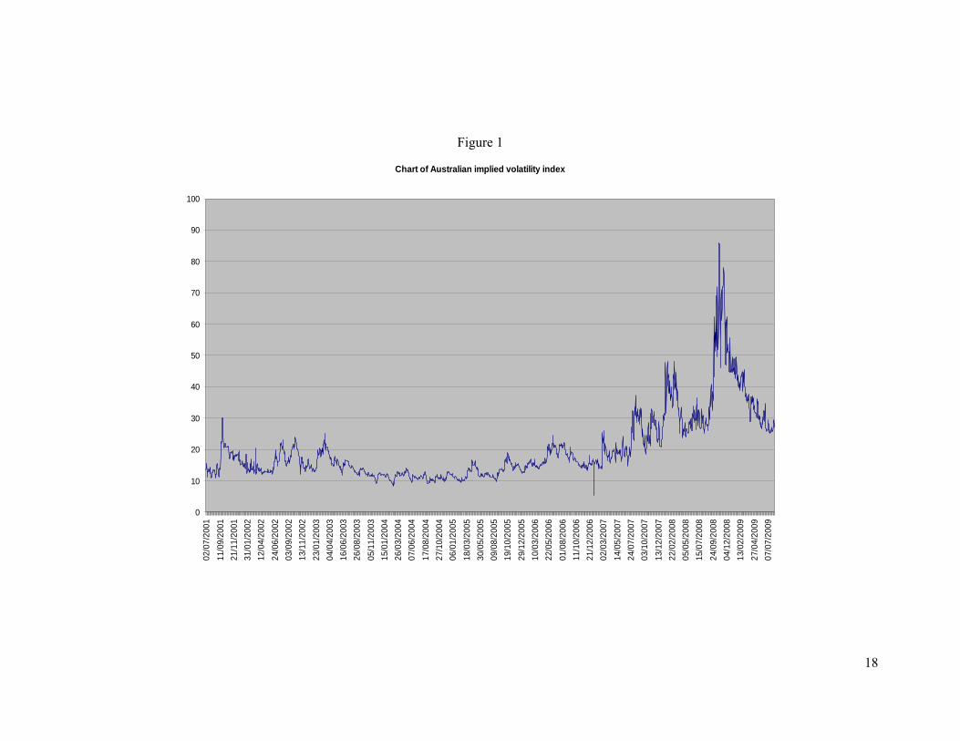
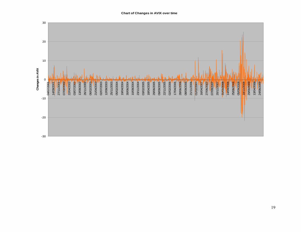
We calculate VIX each trading day using the options on the ASX200 and following the same procedure as Dowling and Muthuswamy (2003). Specifically, we use each day both the two call options and two put contracts that are closest to their exercise date and then take as our measure of VIX the average of the four implied volatilities that we have calculated. The VIX values and changes in these values are reported in Figure 1.

3 (c) Data Selection and Filtering

The only exclusions from our data instances where we gave negative book-to-markets, returns over the announcement period that lie outside of the range of -50% to +50% and NUE is trimmed at the 1st percentile and PUE at the 99th percentile. The final sample after these exclusions is 4,740 announcements. Table 1 reports the statistical

9

properties of this sample divided into the four categories. The absolute values of the NUE and PUE signals are not statistically different, suggesting that the public signals for all four groups are effectively the same. The four categories also do not differ on the other categories reported with the expectation that large increases are more likely to occur at times when the level of VIX is already high. Method

The basic model that we use in our analysis is: Rit = βo + β1 NUEit + β2 PUEit + β3MVit + Year Effects + εit Eq (1) where Rit is the accumulated excess return over the three-day

announcement period which commences the day before the announcement and ends the day after the announcement

NUE = UE if UE < 0; else NUE = 0 PUE = UE if UE > 0; else PUE = 0 MV is the log of the market capitalisation of the firm

Under maxmin expected utility, the proposition is that with no (or little) uncertainty the market reaction to NUE and PUE would be equal (i.e β1 = β2) but when uncertainty is high, then there will be greater reaction to NUE than there will be to PUE (i.e. β1 > β2). We conduct an F-test to determine whether there is any significant difference between β1 and β2. 4. Findings Major Finding

The main focus of the paper is to determine whether the market reaction to earnings announcements is conditioned by the level of uncertainty in the market at the time of the announcement. We report our findings in Table 2 where we expand out basic model by the inclusion of dummy variables in order to measure the market response to bad (PUE) and good (PUE) earnings responses using three different proxies for the level of market uncertainty: (a) change in VIX; (b) level of VIX; (c) both change in VIX and level of VIX.

In each of the three cases the reported coefficients on NUE and PUE provide a

measure of the extent of the market response to the earnings announcements made at times of low uncertainty as measured under each of the three proxies for market uncertainty. The F-stat reported in each case for NUE = PUE clearly establishes that there is no difference in the market response to bad and good earnings news when uncertainty is low4. However, the expected asymmetric response to the earnings announcement at times of high uncertainty is firmly established under all three proxies as indicated by the F stat reported for (a), (b) and (c). In each case the coefficient for NUE (PUE) for high levels of uncertainty are obtained by adding the two coefficients for NUE (PUE). For

4 There is some slight evidence that the investors respond more to good news than they do to bad news when uncertainty is low when measured by both change in VIX and level of VIX (i.e. (c)). We will pursue this possibility later in the paper where we break both changes and levels down into terciles.

10

example, the coefficient for NUE when uncertainty is high under (a) is 0.036 (0.030 +0.006) and for PUE is -0.004 (0.021 – 0.025). What is clear is that regardless of the proxy that we use for market uncertainty, that investors respond strongly to bad news but almost completely ignore good news when it is released at a time of high market uncertainty. The other insight that we should take from Table 2 is that both changes in VIX and the level of VIX both are important in explaining an asymmetric response to earnings announcements. This being the case then in the remainder of this paper we will use a combination of the two as our proxy for uncertainty – high uncertainty being indicated when VIX increases from a high base and low uncertainty being when VIX decreases from a low base. Testing the Robustness of Our Major Finding

In Table 3 we report the report the findings of a series of tests that we conducted to test the robustness of our main finding that investors display increasing pessimism when reacting to earnings announcements as markets become more uncertain. We will next test whether the asymmetric response to earnings announcements at times of high uncertainty In (a) we expand our model to incorporate two characteristics of a firm that have been found to influence its valuations: its size (MV) and its book-to-market (MTBV). Our findings remain unaltered by the introduction of these new variables with the only new term proving significant being the standalone MTBV term which suggests that in all types of markets cheap stocks respond more to all earnings announcements than do more expensive stocks.

One feature of the Australian market is that firms typically make a dividend announcement at the same time that they make an earnings announcement. This raises the possibility that we have incorrectly attributed our previous findings as reflecting the market reaction to good and bad earnings announcements as it may also encompass a reaction to a contemporaneous dividend announcement. In order to investigate this we now add to our basic model, cross product-terms with both NUE and PUE where there is a contemporaneous announcement of either an increase or a decrease in dividends. The results reported in Table 3 (b) confirm our previous main finding on the asymmetry of the markets response to earnings news at times of uncertainty. The one additional insight that we gain being that a dividend increase at a time of a positive earnings announcement negates some of the pessimistic market reaction to such announcements at times of uncertainty, specifically when the uncertainty is at its highest.

Finally, we have used to date last year’s earnings standardised by total assets as our measure of expected earnings (e.g Williams, 2009). Therefore, if this year’s earnings again standardised by total assets is greater (less) than what it was last year, there has been a positive (negative) unexpected earnings which we will designate as PUE (NUE). One deficiency of this measure is that earnings can increase simply as a consequence of the firm increasing its asset base. In order to account for this we also evaluated ROA as measured by earnings divided by average total assets as the benchmark against which to judge whether earnings has increased or not.. We repeat the analysis now using this new measure for expected earnings and our results as reported in Table 3 (c) indicate that the main results still hold and so indicating the robustness of our findings to different definitions of expected earnings.

11

Overall, our further analysis confirms our finding first reported in Table 2 for our basis

model that uncertainty causes an asymmetric response to earnings announcements suggesting that it is priced along with risk. The one other finding worth noting is that in all but one case our previous finding holds that with low uncertainty, there is a significant positive reaction to good news earnings announcements but not to bad news announcements. As in no case are the difference in values of these coefficients significant at times of low uncertainty, the evidence is not strong enough to conclude that investors do diverge from minmax expected uncertainty but we will see more about this when we next investigate finer definitions of low and high uncertainty.

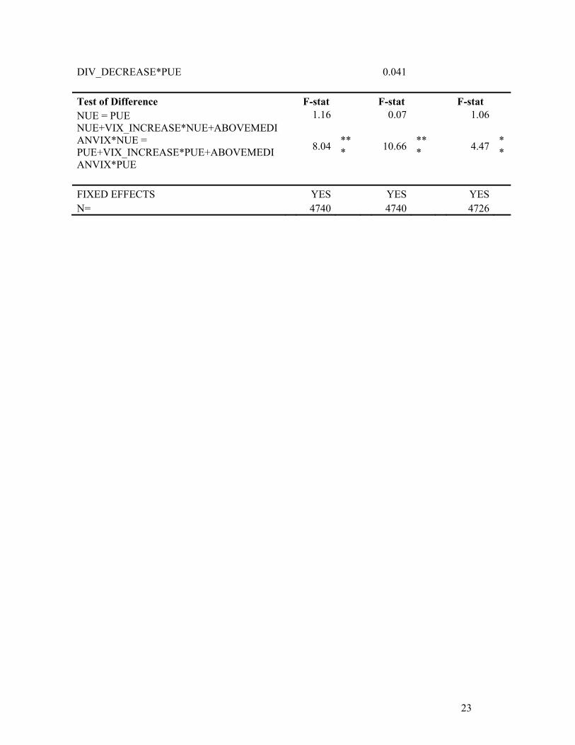
Finer Definitions of Uncertainty The analysis to date has identified at times of high market uncertainty that investors react to bad earnings news but effectively ignore good earnings news. However, using the two-by-two split for VIX changes and VIX levels, we do obtain an inkling that this finding might be reversed at low level of uncertainty. In order to gain a greater insight into this possibility, we undertake a finer breakdown into terciles for both VIX changes and VIX levels. As a consequence, our proxies for uncertainty enable us to classify uncertainty into nine groupings of which we investigate three:

Low uncertainty (large decreases in VIX from an already low level) Medium uncertainty (little or no change in VIX from a median level) High uncertainty (large increases in VIX from an already high level)

We report the results of our analysis in Table 4 and our findings are discussed below:

1) Low Uncertainty: It can be seen that investors react positively to good earnings news (PUE = 0.032**) while they effectively ignore bad news (i.e. NUE = -0.014). Further, this apparent asymmetry in the response is significant with the F-stat = 3.45*. This finding is the opposite to what we have identified previously for times of high uncertainty where investor respond strongly to bad earnings use but effectively ignore god earnings news. In others words, investors appear to display an optimistic best at time of low market uncertainty albeit weaker than the pessimistic bent that they display when market uncertainty is high. This finding questions whether it is appropriate to assume that investors pursue minmax expected utility across the whole range of uncertainty experienced in markets.

2) Median Uncertainty: Where there is little or no change in VIX around a median level, the response coefficient for NUE is 0.045 (-0.014 + 0.072 + -0.003) and for PUE is 0.033 (0.032 -0.007 + 0.008). In other words, investors react strongly and fairly equally to both bad and good news at times of median level of uncertainty. The absence of uncertainty in the response to bad and good news is confirmed by our F-test (= 0.98). This finding mirrors that of Williams (2009) but in his case it was for low uncertainty rather than median uncertainty. We would suggest that the difference is due to Williams only using change in VIX as his proxy for uncertainty which fails to recognise that the level of VIX also plays an important role.

12

3) High Uncertainty: With high uncertainty as measured by large increases in VIX from a high level, the response coefficient for NUE is 0.051(-0.014 +0.019 + 0.046) while that for PUE is -0.031 (0.032 – 0.034 -0.029). The asymmetry between the responses to good and bad news is validated by the highly significant F-test (= 16.55***). It is interesting to note that the main driving force contributing to this uncertainty is that investors react negatively even to good earnings announcements at times of high level of uncertainty.

The conclusion that we can draw to date is that investors do become pessimistic when market uncertainty rises to high levels which is consistent with them pursuing minmax expected uncertainty at such times. However, equally our study of the response of investors to earnings announcements suggests that they typically ignore uncertainty when it is at typical levels and that their attitude switches to one of optimism when market uncertainty is low. As a consequence this study throws into question any asset pricing model that incorporates uncertainty by assuming maxmin expected utility.

Uncertainty and Trading Volume

The basis of uncertainty is that investors lack the relevant information to form unique priors. Dow and Werlang (1992) following a maxmin framework show that uncertainty creates a wedge between buyers and sellers in the market and so reduces the incentives for market participation. Epstein and Schneider (2007) confirm that an increase in uncertainty causes investors to withhold trading but that this will reverse when the uncertainty is resolved. This implies that we can use the level of trading in the market as a measure of the speed of uncertainty resolution which will influence the extent of the asymmetric response to earnings announcements. We would expect that the asymmetric reaction to earnings announcements to be greatest when uncertainty is high and when trading volume is low.

We calculated the abnormal trading volume for the specific stocks (AbVol) which

as the difference between the firm’s trading volume as a percentage of total market volume over the announcement period and the same percentage over the 20 day period prior to the announcement. There are two points that we need to make with respect to this calculation: (i) we are calculating abnormal trading volume at the individual stock level in recognition that for any given level of market uncertainty, the rate of uncertainty resolution at the stock level will differ across stocks; (ii) the value for AbVol that we calculate controls for both the recent level of trading at the stock level and the market level.

This AbVol is used as a dummy variable with stocks being classified into above-

median and below-median trading volume at the time of an earnings announcement. Our findings are reported in Table 5 which confirms previous findings that investors respond similarly to both good and bad earnings announcements when market uncertainty is low (when measured using a two-by-two split for changes in VIX and the level of VIX). They also confirm the asymmetric response when market uncertainty is high and trading volume is low (NUE = 0.058; PUE = -0.32; F-stat = 16.05***). However when the trading volume of a stock remains high during a period of market uncertainty, investors

13

response to both bad and good earnings news in a similar fashion (NUE = 0.032; OPUE = 0.009; F-test = 0.88).

Overall the evidence is supportive of the proposition that uncertainty is

synonymous with lower trading volume and investors respond in an asymmetric way to earnings announcements when our proxy indicates that market uncertainty is high and this is associated with low turnover at the firm level. However, it also indicates that investors respond similarly to bad and good news when they continue to trade at a high volume even if the indicators indicate high market uncertainty. This suggests that stock turnover can be used in concert with the VIX measure to enable us to better identify periods when uncertainty in the market is at high levels.

Uncertainty and Sentiment

The most obvious alternative explanation to uncertainty as providing the explanation for the asymmetric market response to earnings announcements is that it is a reflection of the market sentiment at the time of the announcement. One might expect investor sentiment to erode and for them to abandon markets when they become overly volatile while their sentiment and so their attitude to investing would grow stronger after a period of market stability. Baker and Wurgler (2006) developed a model for measuring the level of investor sentiment towards individual stocks and used this measure to establish that stocks tend to over-react to good news when sentiment is high and over-react to bad news when sentiment is low. This suggests an asymmetric response to announcements when sentiment is both high and low.

Of course, there is the possibility that sentiment can actually combine with uncertainty

when investors determine how to respond to a new information release. The most common proposition in the literature is that investors follow maxmin expected utility when faced with uncertainty meaning that they follow a course of action that seeks to maximise their utility under a worse case outcome. This is just what one might expect when market sentiment is low and so investors are taking a pessimistic view. The question is whether investors will always focus on the worst case outcome when uncertainty comes at a time of high market sentiment. The possibility being that at such times their optimism causes them not to focus on the worst case outcome raising the possibility that sentiment might serve to offset uncertainty and so mitigate the previously found asymmetric response to information at time of high uncertainty (Schroder, 2007).

In order to determine whether market sentiment does play a contributing role in what

seemingly is an asymmetric response to earnings announcements, we introduce two measures for market sentiment: (i) the return momentum of the stock over the five days prior to the announcement which provides a stock specific sentiment measure and (ii) a consumer sentiment measure that is calculated monthly by the Melbourne Institute and Westpac which we use as a proxy for a general market sentiment measure.

To date we have found strong evidence of asymmetry when uncertainty is high and

somewhat weaker evidence when uncertainty is low. We would expect the introduction of sentiment would strengthen these findings when uncertainty and sentiment are in accordance (e.g. high uncertainty and low sentiment) and weaker these findings when they are in conflict

14

(e.g. high uncertainty and high sentiment). In Table 6 we have attempted to summarise the possible market reaction to positive and negative earnings news for combinations of high and low uncertainty with high and low market sentiment.

In order to throw some light on these possibilities we regress all cross-product terms of

uncertainty and sentiment for both positive and negative earnings surprise against he excess returns during the announcement period. We report our findings for the combinations low uncertainty (falling VIX from an already low level) and high uncertainty (rising VIX from an already high level) with low sentiment (below median ) and high sentiment (above median) in Table 7 where momentum is used as proxy fro sentiment (Panel A) and consumer sentiment is used (Panel B).

First looking at periods of high market uncertainty, we find strong evidence using both

proxies for sentiments that the market reacts to bad earnings announcements much more strongly than it does to good earnings announcements when this high uncertainty occurs at a time of low sentiment. This is the asymmetric finding that we have highlighted several times previously that we can attribute to investor pessimism. However during periods when strong sentiment is contemporaneous with high market uncertainty, we find that this asymmetric response to earnings announcement is severely weakened (where momentum is the sentiment proxy) or removed (where consumer sentiment is the sentiment proxy). In other words sentiment works to weaken the investor pessimism that is usually associated with periods of high market uncertainty.

Now looking at periods of low market uncertainty, we find evidence to support that

investors react more to good earnings announcements than they do to bad earnings announcements at times of low sentiment. This asymmetric finding strongly brings into question the extent to which investors take a pessimistic view when faced with any uncertainty. We then come to the anomaly that the asymmetric response that we have just discussed when we combine low uncertainty with low sentiment disappears when we look at periods of low uncertainty and high sentiment. One would have thought that these would be the times of greatest optimism when investors relish good news and dismiss bad news but we find that at such times, markets react similarly to both.

The two findings that we take from this section are (i) sentiment as well as

uncertainty conditions the reactions of investors to information and (ii) that pessimism does not permeate all investor decisions as would be suggested if they pursued minmax expected utility across the spectrum of uncertainty. Of course, we are also left with the mystery as to why strong sentiment have a more positive impact on investor behaviour when it occurs contemporaneously with high market uncertainty. 5. Conclusion It is proposed that uncertainty, rather than risk, provides a much more realistic representation of the setting that we face when we come to pricing asset, and particularly corporate equities. We have gone a long way down the path of developing pricing models that incorporate risk (e.g. CAPM, APT, Fama and French empirical three-factor model)

15

but comparatively little work has been done on the role (if any) that uncertainty plays in asset pricing. In order for uncertainly to affect pricing, it must have some influence on how investors incorporate information into pricing. Our contribution is to evaluate whether uncertainty influences the way by which investors respond to earnings announcements which will provide us with valuable insights as to the role that uncertainty plays in asset pricing. In particular, we evaluate the proposition that investors will follow maxmin expected utility and so will progressively overweight bad news and underweight good news as they become more uncertain. Using VIX as a proxy for market uncertainty and earnings announcements as our information signal, we find that there is an asymmetric response to good and bad earnings news at high levels of uncertainty which is consistent with uncertainty breeding pessimism in the minds of investors. However, we do find evidence to suggest investors might have a more optimistic bent than is allowed under maxmin expected utility as indicated by how they react to earnings announcements when uncertainty is at the lower end of the scale.

Other factors that we have found to influence the extent of the pessimistic response to information associated with uncertainty are the prevailing level to market sentiment, whether it releases a confirming dividend announcement at the time of releasing good earnings news and the existing valuation of the stock as reflected by its book-to-market ratio. All of these finding lead us to question to which investors consistently apply maxmin expected utility when faced with uncertainty. We also find that the level of trading around the announcement date has implications for the market reaction to information signals conditioned by uncertainty. However, in this case, there is good reason to believe that the impact of the announcement on volume is also an outworking of uncertainty and, indeed, provides a good secondary indicator when attempting to classify the level of market uncertainty at any point in time.

Much more remains to be done but two matters that we are particularly interested to address is (i) the extent to which certain firms/industries are more susceptible than others to exhibiting an asymmetric to information release information and (ii) whether the asymmetry gives rise to exploitable investment opportunities. On this latter point, the evidence suggests that market uncertainty is transitory which suggests that any influence that it has on market prices will ebb and flow. This suggest that investing in stocks who deliver good news at a time of high uncertainty (and low market confidence) may deliver excess returns but, of course, it is a bet on how long it will take for this uncertainty (and sentiment) to recover. (iii) Prior evidence has shown that uncertainty can cause greater post earnings announcement drift. Our finding of asymmetric reaction to earnings news leads us to ponder the possibility of an asymmetric post earnings announcement drift. Finally, more work needs to be done on looking at the association between uncertainty and sentiment and especially to resolve the anomaly where higher sentiment seems to negate optimism at times of low uncertainty.

16

References Al-Najjar, N.I., and J. Weinstein, 2009. “The Ambiguity Aversion Literature: A Critical

Assessment” Economics and Philosophy 25: 249–284. Anderson, E.W., E. Ghysels and J.L. Juergens, 2009. “The impact of risk and

uncertainty on expected returns.” Journal of Financial Economics 94(2): 233-263. Baker, M. and J. Wurgler. 2007. “Investor sentiment in the stock market.” Journal of

Economic Perspectives 21(2): 129-151. Ball, R., and P. Brown. 1968. “An Empirical Evaluation of Accounting Income Numbers.”

Journal of Accounting Research 6: 159-177. Becker, S.W. and F.O. Brownson. 1964. “What Price Ambiguity? Or the Role of Ambiguity in Decision-Making.” Journal of Political Economy 72(1): 62-73. Carr, P., and L. Wu, 2009. “Variance Risk Premia.” Review of Financial Studies 22(3):

1311-1341. Caskey, J. A. 2008. “Information in Equity Markets with Ambiguity Averse Investors.”

Review of Financial Studies, forthcoming. Chen, Z. and L.G. Epstein, 2002. “Ambiguity, risk and asset returns in continuous time.”

Econometrica 70: 1403-1443. Daniel, K., D. Hirshleifer and A. Subrahmanyam, 1998. “Investor psychology and

security market over- and under-reactions.” Journal of Finance 53 (6): 1839-1886. Dow, J. and S. R. C. Werlang. 1992. “Uncertainty Aversion and the Optimal Choice of

Portfolio.” Econometrica 60: 197-204. Dowling, S. and J. Muthuswamy. 2003. “The Implied Volatility of Australian Index

Options.” Working Paper. University of Sydney. Drechsler, I. 2008. “Uncertainty, Time-Varying Fear, and Asset Prices.” Working Paper,

The Wharton School, University of Pennsylvania. Easley, D and M. O’Hara, 2008. “Liquidity and Valuation in an Uncertain World.”

Working Paper, Cornell University. Ellsberg, D. 1961. “Risk, Ambiguity, and the Savage Axioms.” Quarterly Journal of

Economics 75: 643-669. Epstein L. G., and M. Schneider, 2010. “Ambiguity and Asset Markets.” Working paper.

Available from http://128.197.153.21/lepstein/files-research/NBER-Jan20.pdf Epstein, L. G. and M. Schneider. 2003. “Recursive multiple-priors.” Journal of Economic

Theory 113: 1-31. Epstein, L. G. and M. Schneider. 2008, “Ambiguity, Information Quality and Asset

Pricing.” Journal of Finance 63: 197-228. Eraker, B., 2004, “Do Equity Prices and Volatility Jump? Reconciling Evidence from

Spot and Option Prices.” Journal of Finance 56(3), 1367-1403. Gilboa, I. and D. Schmeidler. 1989. “Maxmin Expected Utility with Non-Unique Prior.”

Journal of Mathematical Economics 18: 141-153. Gysler, M, J. B. Kruse and R. Schubert. 2002. “Ambiguity and Gender differences in

financial decisions making: An experimental examination of competence and confidence effects.” Working Paper. Swiss Federal Institute of Technology.

Hansen, L. P. and T. J. Sargent. 2008. “Fragile beliefs and the price of model uncertainty.” Working Paper, University of Chicago.

17

Heath,C. and A. Tversky, 1991. “Preference and Belief: Ambiguity and Competence in Choice under Uncertainty.” Journal of Risk and Uncertainty 4: 5-28.

Jiang, G., C.M.C. Lee and G.Y. Zhang, 2005. ‘‘Information Uncertainty and Expected Returns.’’ Review of Accounting Studies 10(2-3): 185-221.

Jones, C.P. and R.H. Litzenberger, 1970. “Quarterly Earnings Reports and Intermediate Stock Price Trends.” The Journal of Finance, Vol. 25(1): 143-148.

Joy, M., R. Litzenberger, and R. McEnally, 1997. “The Adjustment of Stock Prices to Announcements of Unanticipated Changes in Quarterly Earnings,” Journal of Accounting Research: 207-225.

Keynes, J. M. 1937. “The General Theory of Employment.” Quarterly Journal of Economics, 51: 209-23?

Knight, F. H. 1921. Risk, Uncertainty and Profit. Boston: Houghton Mifflin Company. MacCrimmon, K.R. and S. Larsson. 1979. “Utility Theory: Axioms versus ~Paradoxes.” "In M. Allais and O. Hagen (eds.), Expected Utility and the Allais Paradox. Dordrecht, Holland: D. Reidel: 333-409. Ozoguz, A. 2009. “Good Times or Bad Times? Investors’ Uncertainty and Stock Returns.”

Review of Financial Studies 22(11): 4377-4422. Rendleman, Jr., R. J., C. P. Jones, and H. A. Latané. 1987. “Further insight into the

standardized unexpected earnings anomaly: size and serial correlation effects.” The Financial Review 22(1): 131-144.

Schroder, D. 2007. “Investment under Ambiguity with the Best and the Worst in Mind.” Working Paper. Bonn Graduate School of Economics.

Slovic, P. and A. Tversky. (1974). "Who Accepts Savage's Axiom?" Behavioral Science 19(6): 368-373. Williams, C.D. 2009. “Asymmetric Responses to Earnings News: A case od Ambiguity.”

Working Paper, University of North Carolina. Zhang , X. Frank. 2006, Information Uncertainty and Stock Returns , Journal of Finance

61 (1): 105-137.

18

Figure 1

Chart of Australian implied volatility index

0

10

20

30

40

50

60

70

80

90

10002

/07/

2001

11/0

9/20

01

21/1

1/20

01

31/0

1/20

02

12/0

4/20

02

24/0

6/20

02

03/0

9/20

02

13/1

1/20

02

23/0

1/20

03

04/0

4/20

03

16/0

6/20

03

26/0

8/20

03

05/1

1/20

03

15/0

1/20

04

26/0

3/20

04

07/0

6/20

04

17/0

8/20

04

27/1

0/20

04

06/0

1/20

05

18/0

3/20

05

30/0

5/20

05

09/0

8/20

05

19/1

0/20

05

29/1

2/20

05

10/0

3/20

06

22/0

5/20

06

01/0

8/20

06

11/1

0/20

06

21/1

2/20

06

02/0

3/20

07

14/0

5/20

07

24/0

7/20

07

03/1

0/20

07

13/1

2/20

07

22/0

2/20

08

05/0

5/20

08

15/0

7/20

08

24/0

9/20

08

04/1

2/20

08

13/0

2/20

09

27/0

4/20

09

07/0

7/20

09

19

Chart of Changes in AVIX over time

-30

-20

-10

0

10

20

30

04/0

7/20

01

14/0

9/20

01

27/1

1/20

01

07/0

2/20

02

22/0

4/20

02

03/0

7/20

02

13/0

9/20

02

26/1

1/20

02

06/0

2/20

03

21/0

4/20

03

02/0

7/20

03

12/0

9/20

03

25/1

1/20

03

05/0

2/20

04

19/0

4/20

04

30/0

6/20

04

10/0

9/20

04

23/1

1/20

04

03/0

2/20

05

18/0

4/20

05

29/0

6/20

05

09/0

9/20

05

22/1

1/20

05

02/0

2/20

06

17/0

4/20

06

28/0

6/20

06

08/0

9/20

06

21/1

1/20

06

01/0

2/20

07

16/0

4/20

07

27/0

6/20

07

07/0

9/20

07

20/1

1/20

07

31/0

1/20

08

14/0

4/20

08

25/0

6/20

08

05/0

9/20

08

18/1

1/20

08

29/0

1/20

09

13/0

4/20

09

24/0

6/20

09

Cha

nges

in A

VIX

20

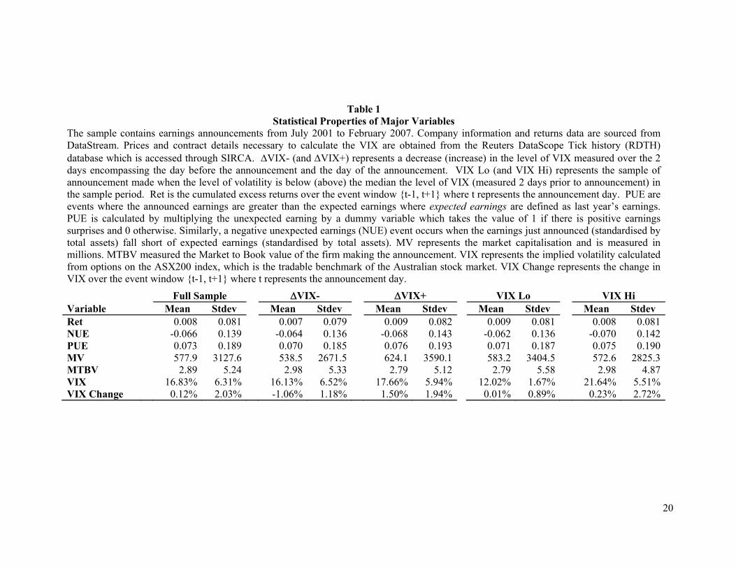
Table 1 Statistical Properties of Major Variables

The sample contains earnings announcements from July 2001 to February 2007. Company information and returns data are sourced from DataStream. Prices and contract details necessary to calculate the VIX are obtained from the Reuters DataScope Tick history (RDTH) database which is accessed through SIRCA. VIX- (and VIX+) represents a decrease (increase) in the level of VIX measured over the 2 days encompassing the day before the announcement and the day of the announcement. VIX Lo (and VIX Hi) represents the sample of announcement made when the level of volatility is below (above) the median the level of VIX (measured 2 days prior to announcement) in the sample period. Ret is the cumulated excess returns over the event window {t-1, t+1} where t represents the announcement day. PUE are events where the announced earnings are greater than the expected earnings where expected earnings are defined as last year’s earnings. PUE is calculated by multiplying the unexpected earning by a dummy variable which takes the value of 1 if there is positive earnings surprises and 0 otherwise. Similarly, a negative unexpected earnings (NUE) event occurs when the earnings just announced (standardised by total assets) fall short of expected earnings (standardised by total assets). MV represents the market capitalisation and is measured in millions. MTBV measured the Market to Book value of the firm making the announcement. VIX represents the implied volatility calculated from options on the ASX200 index, which is the tradable benchmark of the Australian stock market. VIX Change represents the change in VIX over the event window {t-1, t+1} where t represents the announcement day.

Full Sample VIX- VIX+ VIX Lo VIX Hi Variable Mean Stdev Mean Stdev Mean Stdev Mean Stdev Mean Stdev Ret 0.008 0.081 0.007 0.079 0.009 0.082 0.009 0.081 0.008 0.081NUE -0.066 0.139 -0.064 0.136 -0.068 0.143 -0.062 0.136 -0.070 0.142PUE 0.073 0.189 0.070 0.185 0.076 0.193 0.071 0.187 0.075 0.190MV 577.9 3127.6 538.5 2671.5 624.1 3590.1 583.2 3404.5 572.6 2825.3MTBV 2.89 5.24 2.98 5.33 2.79 5.12 2.79 5.58 2.98 4.87VIX 16.83% 6.31% 16.13% 6.52% 17.66% 5.94% 12.02% 1.67% 21.64% 5.51%VIX Change 0.12% 2.03% -1.06% 1.18% 1.50% 1.94% 0.01% 0.89% 0.23% 2.72%

21

Table 2 Investors’ reaction to Earnings announcement by changes in Uncertainty (∆VIX) and VIX

level The sample contains earnings announcements from July 2001 to February 2007. The dependent variable is the cumulated excess returns over the event window {t-1, t+1} where t represents the announcement day. VIX represents the implied volatility calculated from options on the ASX200 index, which is the tradable benchmark of the Australian stock market. VIX_INCREASE is an indicator variable that takes the value of 1 when the earnings announcement occurs in an event window where an increase in the level of VIX and 0 otherwise. ABOVEMEDIANVIX is an indicator variable that takes the value of 1 when the earnings announcement occurs when the VIX level is above the median VIX level over the sample period and 0 otherwise. PUE is calculated by multiplying the unexpected earning by a dummy variable which takes the value of 1 if there is positive earnings surprises and 0 otherwise. Similarly, a negative unexpected earnings (NUE) event occurs when the earnings just announced (standardised by total assets) fall short of expected earnings (standardised by total assets). MV represents the market capitalisation and is measured in millions. Fixed Effects refers to year dummy variables which are included (but not reported) in the regression. The notations ***, ** and * denotes statistical significance at the 1%, 5% and 10% level respectively. (a) (b) (c)

Variable Coefficient

s Coefficient

s Coefficient

s

NUE 0.030*** 0.018 0.018

PUE 0.021 ** 0.022 ** 0.030***

MV 0.000 0.000 0.000 VIX_INCREASE*NUE 0.006 0.000 VIX_INCREASE*PUE -0.025 ** -0.021 * ABOVEMEDIANVIX*NUE 0.029 * 0.029 * ABOVEMEDIANVIX*PUE -0.026 ** -0.021 * Test of Difference F-stat F-stat F-stat NUE = PUE 0.38 0.06 0.42 NUE+VIX_INCREASE*NUE =PUE+VIX_INCREASE*PUE 6.93

***

NUE+ABOVEMEDIANVIX*NUE = PUE+ABOVEMEDIANVIX*PUE 10.47

***

NUE+VIX_INCREASE*NUE+ABOVEMEDIANVIX*NUE = PUE+VIX_INCREASE*PUE+ABOVEMEDIANVIX*PUE

11.38***

FIXED EFFECTS YES YES YES N= 4740 4740 4740

22

TABLE 3 Expanded model results of investors’ reaction to Earnings announcement changes in

Uncertainty (∆VIX) and Level of Uncertainty

The sample contains earnings announcements from July 2001 to February 2007. The dependent variable is the cumulated excess returns over the event window {t-1, t+1} where t represents the announcement day. VIX represents the implied volatility calculated from options on the ASX200 index, which is the tradable benchmark of the Australian stock market. VIX_INCREASE is an indicator variable that takes the value of 1 when the earnings announcement occurs in an event window where an increase in the level of VIX and 0 otherwise. ABOVEMEDIANVIX is an indicator variable that takes the value of 1 when the earnings announcement occurs when the VIX level is above the median VIX level over the sample period and 0 otherwise. PUE is calculated by multiplying the unexpected earning by a dummy variable which takes the value of 1 if there is positive earnings surprises and 0 otherwise. Similarly, a negative unexpected earnings (NUE) event occurs when the earnings just announced (standardised by total assets) fall short of expected earnings (standardised by total assets). For (c), a different definition is employed for unexpected earnings. In this regression, a PUE event occurs when there is an increase in ROA. PUE is calculated by multiplying the change in ROA i.e. (ROA t – ROA t-1)/ROAt-1 by a dummy variable which takes the value of 1 if there is positive earnings surprises and 0 otherwise. Similarly negative unexpected earnings (NUE) occur when there is a fall in ROA. MV represents the market capitalisation and is measured in millions. MTBV measured the Market to Book value of the firm making the announcement. Div Decrease is a dummy variable equal to 1 when there is a decrease in final dividends and 0 otherwise. Similarly Div Increase is equal to 1 when final dividend increases from the previous year and 0 otherwise. Fixed Effects refers to year dummy variables which are included (but not reported) in the regression. The notations ***, ** and * denotes statistical significance at the 1%, 5% and 10% level respectively. (a) (b) (c)

Variable Coefficients Coefficients CoefficientsNUE 0.015 0.015 0.000

PUE 0.036*** 0.020 * 0.020 *

MV 0.000 0.000 0.000 VIX_INCREASE*NUE 0.001 0.001 0.019 VIX_INCREASE*PUE -0.022 * -0.019 -0.010 ABOVEMEDIANVIX*NUE 0.028 0.028 * 0.028 * ABOVEMEDIANVIX*PUE -0.021 * -0.015 -0.005 MV*NUE 0.000 MV*PUE 0.000 MTBV -0.001 * MTBV*NUE 0.000 MTBV*PUE 0.000 DIV_INCREASE*NUE 0.015

DIV_INCREASE*PUE 0.066 ***

DIV_DECREASE*NUE -0.029

23

DIV_DECREASE*PUE 0.041

Test of Difference F-stat F-stat F-stat NUE = PUE 1.16 0.07 1.06 NUE+VIX_INCREASE*NUE+ABOVEMEDIANVIX*NUE = PUE+VIX_INCREASE*PUE+ABOVEMEDIANVIX*PUE

8.04***

10.66 ***

4.47**

FIXED EFFECTS YES YES YES N= 4740 4740 4726

24

Table 4

Response to earning surprises with Tercile dummies representing differing levels of VIX and changes in VIX

The sample contains earnings announcements from July 2001 to February 2007. The dependent variable is the cumulated excess returns over the event window {t-1, t+1} where t represents the announcement day. PUE is calculated by multiplying the unexpected earning by a dummy variable which takes the value of 1 if there is positive earnings surprises and 0 otherwise. Similarly, a negative unexpected earnings (NUE) event occurs when the earnings just announced (standardised by total assets) fall short of expected earnings (standardised by total assets). In this regression, we formed dummy variable by splitting the sample into 3 terciles based on the changes in VIX during the event window. TER2CHANGE is a dummy variable which takes a value of 1 when the earnings announcement occurs in the middle tercile based on changes in VIX. Otherwise TER2CHANGE will be 0. Similarly TER3CHANGE is a dummy variable which takes a value of 1 when the earnings announcement occurs in the tercile of largest changes in VIX and 0 otherwise. The regression also incorporates indicator variable that is formed based on the VIX level at the time of announcement. The sample is sorted into terciles based on the level of VIX 2 days prior to announcement. TER2LEVEL and TER3LEVEL are dummy variable that indicates that the announcement occurs at “medium” and “high” level of VIX respectively. Fixed Effects refers to year dummy variables which are included (but not reported) in the regression. The notations ***, ** and * denotes statistical significance at the 1%, 5% and 10% level respectively.

Coefficients NUE -0.014 PUE 0.032 ** MV 0.000 TER2CHANGE*NUE 0.072 ***TER2CHANGE*PUE -0.007 TER3CHANGE*NUE 0.019 TER3CHANGE*PUE -0.034 ** TER2LEVEL*NUE -0.003 TER2LEVEL*PUE 0.008 TER3LEVEL*NUE 0.046 ** TER3LEVEL*PUE -0.029 * Test of Difference F-stat NUE = PUE 3.45 * NUE+TER2CHANGE*NUE+TER2LEVEL*NUE = PUE+TER2CHANGE*PUE+TER2LEVEL*PUE

0.98

NUE+TER3CHANGE*NUE+TER3LEVEL*NUE = PUE+TER3CHANGE*PUE+TER3LEVEL*PUE

16.55 ***

FIXED EFFECTS YES N= 4740

25

Table 5 The impact of trading on Investors’ reaction to Earnings announcement

The sample contains earnings announcements from July 2001 to February 2007. The dependent variable is the cumulated excess returns over the event window {t-1, t+1} where t represents the announcement day. ABOVEMEDIANVIX is an indicator variable that takes the value of 1 when the earnings announcement occurs when the VIX level is above the median VIX level over the sample period and 0 otherwise. ABOVEMEDIANVOLUME is a dummy variable which takes a value of 1 when the firm level of trading is above the sample median trading volume. Trading volume is calculated by the difference between the firm’s trading volume as a percentage of total market volume and the average percentage of traded estimated in a 20 day period leading to the announcement. Fixed Effects refers to year dummy variables which are included (but not reported) in the regression. The notations ***, ** and * denotes statistical significance at the 1%, 5% and 10% level respectively. Variable Coefficients NUE 0.029 * PUE 0.016 MV 0.000 VIX_INCREASE*NUE 0.002 VIX_INCREASE*PUE -0.023 * ABOVEMEDIANVIX*NUE 0.027 ABOVEMEDIANVIX*PUE -0.025 * ABOVEMEDIANVOLUME*NUE -0.026 ABOVEMEDIANVOLUME*PUE 0.041 *** Test of Difference NUE = PUE 0.33 ABOVEMEDIANVOLUME*NUE = ABOVEMEDIANVOLUME*PUE 14.19 ***NUE+VIX_INCREASE*NUE+ABOVEMEDIANVIX*NUE = PUE+VIX_INCREASE*PUE+ABOVEMEDIANVIX*PUE

16.05 ***

NUE+VIX_INCREASE*NUE+ABOVEMEDIANVIX*NUE+ABOVEMEDIANVOLUME*NUE = PUE+VIX_INCREASE*PUE+ABOVEMEDIANVIX*PUE+ABOVEMEDIANVOLUME*PUE

0.88

FIXED EFFECTS YES N= 4740

26

Table 6

Possible Markets Response to Earning’s Announcements

Classified by Uncertainty and Sentiment

Sentiment Uncertainty Low High

Low

Uncertain, but possibly a slightly greater reaction to

PUE or NUE

Expect that the reaction to PUE would be greater than that to NUE

High

Expect that the reaction to NUE would be greater than that to PUE

Uncertain, but possibly a slightly great reaction to NUE than PUE

27

Table 7 Impact of sentiment and momentum on Investors’ reaction to Earnings announcement

The sample contains earnings announcements from July 2001 to February 2007. The dependent variable is the cumulated excess returns over the event window {t-1, t+1} where t represents the announcement day. The following table reports the results of regression that highlights the reaction to unexpected earnings announcements in the various climates of uncertainty. The sample is split into VIX level terciles based on the level of VIX 2 days prior to announcements. LOWVIX is a dummy variable that takes a value of 1 when the observation falls into tercile of lowest VIX level. HIGHVIX is a dummy variable that takes a value of 1 when the observation occurs when VIX is in the high tercile. Similarly the sample is sorted according to the changes in VIX and terciles were formed. LOWVIX is a dummy variable that takes a value of 1 when the observation falls into tercile of lowest VIX level. HIGHVIX is a dummy variable that takes a value of 1 when the observation occurs when VIX is in the high tercile. In both regressions, we have included each segment of uncertainty as independent variables. However we will only report the extreme segments of greatest uncertainty (HIGHVIX/HIGHCHANGE) and least uncertainty (LOWVIX/LOWCHANGE). In panel A, we examine whether the momentum of the market impacts on the reaction to uncertainty. HIGHMOMENTUM is a dummy variable that takes a value of 1 if the markets return (in the five days prior to the event window) is greater than the median. LOWMOMENTUM is a dummy variable that takes a value of 1 if the markets return (in the five days prior to the event window) is below the median Similarly in panel B, we examine whether Sentiment plays a role in reaction to unexpected earnings under uncertainty. HIGHSENTIMENT is a dummy variable that takes a value of 1 if the announcement occurs when the sentiment index is above the median and 0 otherwise. Conversely LOWSENTIMENT takes a value of 1 if the announcement is made when sentiment is below the median level. Fixed Effects refers to year dummy variables which are included (but not reported). The notations ***, ** and * denotes statistical significance at the 1%, 5% and 10% level respectively.

PANEL A Variable Coefficients MV 0.000 LOWVIX*LOWCHANGE*HIGHMOMENTUM*NUE -0.036 LOWVIX*LOWCHANGE*HIGHMOMENTUM*PUE -0.009 LOWVIX*LOWCHANGE*LOWMOMENTUM*NUE -0.121 ** LOWVIX*LOWCHANGE*LOWMOMENTUM*PUE 0.124 ***HIGHVIX*HIGHCHANGE*HIGHMOMENTUM*NUE 0.060 HIGHVIX*HIGHCHANGE*HIGHMOMENTUM*PUE -0.051 HIGHVIX*HIGHCHANGE*LOWMOMENTUM*NUE 0.059 ***HIGHVIX*HIGHCHANGE*LOWMOMENTUM*PUE -0.046 ** Test of difference: LOWVIX*LOWCHANGE*HIGHMOMENTUM*NUE = LOWVIX*LOWCHANGE*HIGHMOMENTUM*PUE

0.49

LOWVIX*LOWCHANGE*LOWMOMENTUM*NUE = LOWVIX*LOWCHANGE*LOWMOMENTUM*PUE

10.43 ***

HIGHVIX*HIGHCHANGE*HIGHMOMENTUM*NUE = HIGHVIX*HIGHCHANGE*HIGHMOMENTUM*PUE

4.76 *

HIGHVIX*HIGHCHANGE*LOWMOMENTUM*NUE = HIGHVIX*HIGHCHANGE*LOWMOMENTUM*PUE

13.00 ***

28

FIXED EFFECTS YES

Panel B Variable Coefficients MV 0.000 LOWVIX*LOWCHANGE*HIGHSENTIMENT*NUE -0.003 LOWVIX*LOWCHANGE*HIGHSENTIMENT*PUE 0.007 LOWVIX*LOWCHANGE*LOWSENTIMENT*NUE 0.015 LOWVIX*LOWCHANGE*LOWSENTIMENT*PUE 0.418 ** HIGHVIX*HIGHCHANGE*HIGHSENTIMENT*NUE -0.068 HIGHVIX*HIGHCHANGE*HIGHSENTIMENT*PUE -0.034 HIGHVIX*HIGHCHANGE*LOWSENTIMENT*NUE 0.059 ** HIGHVIX*HIGHCHANGE*LOWSENTIMENT*PUE -0.044 ** Test of difference: LOWVIX*LOWCHANGE*HIGHSENTIMENT*NUE = LOWVIX*LOWCHANGE*HIGHSENTIMENT*PUE

0.08

LOWVIX*LOWCHANGE*LOWSENTIMENT*NUE = LOWVIX*LOWCHANGE*LOWSENTIMENT*PUE

4.63 **

HIGHVIX*HIGHCHANGE*HIGHSENTIMENT*NUE = HIGHVIX*HIGHCHANGE*HIGHSENTIMENT*PUE

0.20

HIGHVIX*HIGHCHANGE*LOWSENTIMENT*NUE = HIGHVIX*HIGHCHANGE*LOWSENTIMENT*PUE

8.58 ***

FIXED EFFECTS YES